tecnical animation

8/14/2019 tecnical animation

http://slidepdf.com/reader/full/tecnical-animation 1/13

Cross Section Volume 1 (2007)

http://dewey.weber.edu/crossection/

Probing the Effects of Alternate Jupiters

on the Inner Planets with Blender 3D

Ron Proctor, Department of Physics, Weber State University

Abstract: While the consequences of an alternate Jovian position and mass are generallyunderstood, it seems that the nature of gravity on an astronomical scale is not. We

believe an improvement in visualization techniques can address this problem. Wepropose the creation of an interactive solution, in which a model of the inner solar systemand Jupiter is simulated. It is believed that, through manipulation of the model(changing the mass, position, and other properties of Jupiter), a learner might gaingreater understanding of gravity on an astronomical scale..

INTRODUCTION

The question, “what happens if we do this?” is best answered with manipulation,exploration, and observation. When given a physical model of a complex system (such as theSun-Earth-Moon System), it has been shown that students are better able to learn correctexplanations for observed phenomena (e.g. Phases of the Moon) (Trundle, et al. 2001). If a

concept can be transformed into something we can touch and see, we stand a much betterchance of understanding the system.It turns out that some systems are difficult to produce as tabletop kits. The gravitational

interactions of massive bodies is one example. In this case, a virtual model is more appropriate(and safer) for classroom or museum use.

Using Blender 3D and Python Scripting, we have produced a model of the inner solarsystem plus Jupiter. Though still under development, our code allows the user to change theorbital properties and mass of Jupiter, run a simulation to find out what happens, record theoutput of the simulation for playback, and does this while visualizing the system in threedimensions as the calculation progresses.



74 R. Proctor

Cross Section 2007

Introducing Blender 3D

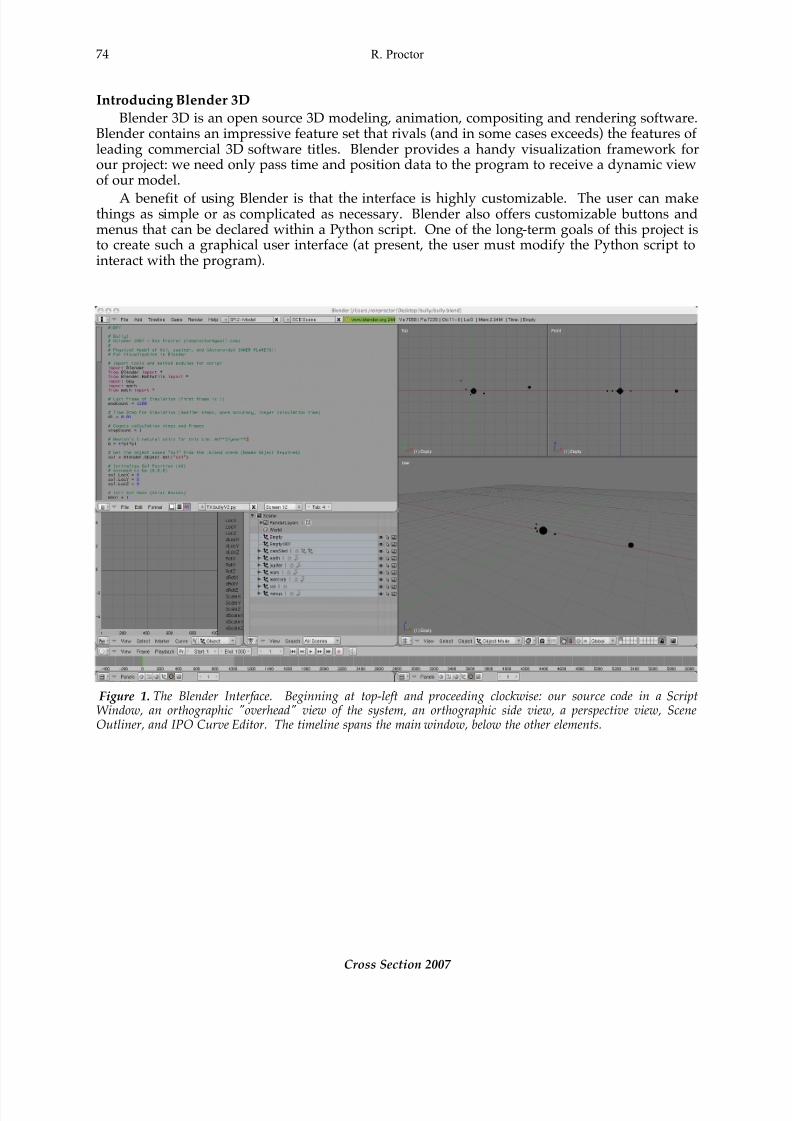
Blender 3D is an open source 3D modeling, animation, compositing and rendering software.Blender contains an impressive feature set that rivals (and in some cases exceeds) the features of leading commercial 3D software titles. Blender provides a handy visualization framework forour project: we need only pass time and position data to the program to receive a dynamic viewof our model.

A benefit of using Blender is that the interface is highly customizable. The user can makethings as simple or as complicated as necessary. Blender also offers customizable buttons andmenus that can be declared within a Python script. One of the long-term goals of this project isto create such a graphical user interface (at present, the user must modify the Python script tointeract with the program).

Figure 1. The Blender Interface. Beginning at top-left and proceeding clockwise: our source code in a ScriptWindow, an orthographic "overhead" view of the system, an orthographic side view, a perspective view, SceneOutliner, and IPO Curve Editor. The timeline spans the main window, below the other elements.



Probing the Effects of Alternate Jupiters on the Inner Planets with Blender 3D 75


METHODS Our simulation code is written in Python, a high-level programming language (named for

the British comedy troupe, not the snake). Python focuses on being human-readable, meaningthat anyone with a basic understanding of programming should be able to work out what thesource code is trying to do (and fix the various errors features of the code).

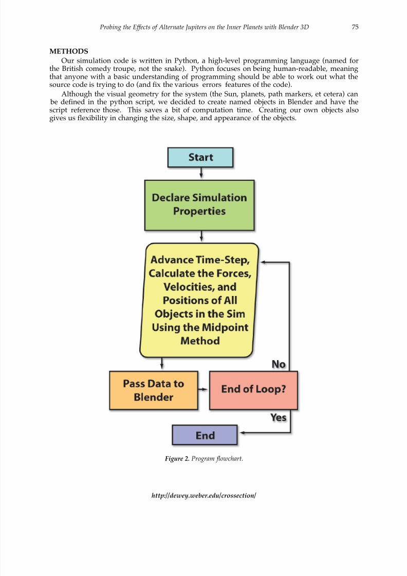
Although the visual geometry for the system (the Sun, planets, path markers, et cetera) can

be defined in the python script, we decided to create named objects in Blender and have thescript reference those. This saves a bit of computation time. Creating our own objects alsogives us flexibility in changing the size, shape, and appearance of the objects.

Figure 2. Program flowchart.



76 R. Proctor

Cross Section 2007

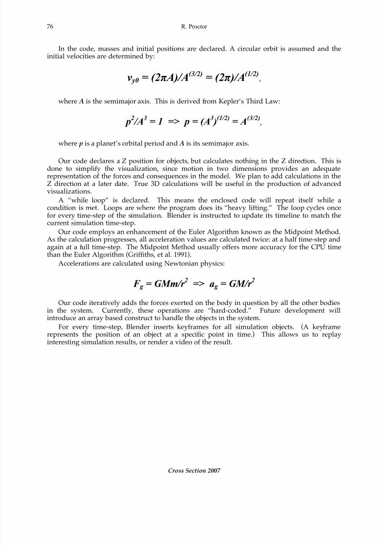
In the code, masses and initial positions are declared. A circular orbit is assumed and theinitial velocities are determined by:

v y0 = (2π A)/A(3/2) = (2π )/A(1/2),

where A is the semimajor axis. This is derived from Kepler’s Third Law:

p2 /A

3= 1 => p = (A

3 )

(1/2)= A

(3/2),

where p is a planet’s orbital period and A is its semimajor axis.

Our code declares a Z position for objects, but calculates nothing in the Z direction. This isdone to simplify the visualization, since motion in two dimensions provides an adequaterepresentation of the forces and consequences in the model. We plan to add calculations in theZ direction at a later date. True 3D calculations will be useful in the production of advanced

visualizations.A “while loop” is declared. This means the enclosed code will repeat itself while a

condition is met. Loops are where the program does its “heavy lifting.” The loop cycles oncefor every time-step of the simulation. Blender is instructed to update its timeline to match thecurrent simulation time-step.

Our code employs an enhancement of the Euler Algorithm known as the Midpoint Method.As the calculation progresses, all acceleration values are calculated twice: at a half time-step andagain at a full time-step. The Midpoint Method usually offers more accuracy for the CPU timethan the Euler Algorithm (Griffiths, et al. 1991).

Accelerations are calculated using Newtonian physics:

F g = GMm/r

2

=> a g = GM/r

2

Our code iteratively adds the forces exerted on the body in question by all the other bodiesin the system. Currently, these operations are “hard-coded.” Future development willintroduce an array based construct to handle the objects in the system.

For every time-step, Blender inserts keyframes for all simulation objects. (A keyframerepresents the position of an object at a specific point in time.) This allows us to replayinteresting simulation results, or render a video of the result.





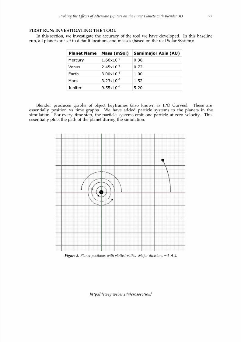
FIRST RUN: INVESTIGATING THE TOOL In this section, we investigate the accuracy of the tool we have developed. In this baseline

run, all planets are set to default locations and masses (based on the real Solar System):

Planet Name Mass (mSol) Semimajor Axis (AU)

Mercury 1.66x10-7

0.38

Venus 2.45x10-6

0.72

Earth 3.00x10-6

1.00

Mars 3.23x10-7

1.52

Jupiter 9.55x10-4

5.20

Blender produces graphs of object keyframes (also known as IPO Curves). These areessentially position vs time graphs. We have added particle systems to the planets in thesimulation. For every time-step, the particle systems emit one particle at zero velocity. This

essentially plots the path of the planet during the simulation.

Figure 3. Planet positions with plotted paths. Major divisions = 1 AU.



78 R. Proctor

Cross Section 2007

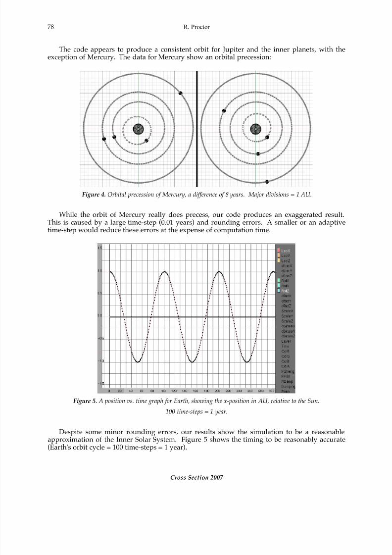
The code appears to produce a consistent orbit for Jupiter and the inner planets, with theexception of Mercury. The data for Mercury show an orbital precession:

Figure 4. Orbital precession of Mercury, a difference of 8 years. Major divisions = 1 AU.

While the orbit of Mercury really does precess, our code produces an exaggerated result.This is caused by a large time-step (0.01 years) and rounding errors. A smaller or an adaptivetime-step would reduce these errors at the expense of computation time.

Figure 5. A position vs. time graph for Earth, showing the x-position in AU, relative to the Sun.

100 time-steps = 1 year.

Despite some minor rounding errors, our results show the simulation to be a reasonableapproximation of the Inner Solar System. Figure 5 shows the timing to be reasonably accurate(Earth's orbit cycle = 100 time-steps = 1 year).





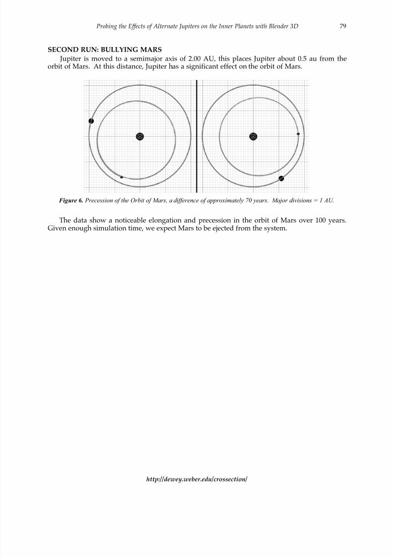
SECOND RUN: BULLYING MARS Jupiter is moved to a semimajor axis of 2.00 AU, this places Jupiter about 0.5 au from the

orbit of Mars. At this distance, Jupiter has a significant effect on the orbit of Mars.

Figure 6. Precession of the Orbit of Mars, a difference of approximately 70 years. Major divisions = 1 AU.

The data show a noticeable elongation and precession in the orbit of Mars over 100 years.Given enough simulation time, we expect Mars to be ejected from the system.



80 R. Proctor

Cross Section 2007

THIRD RUN: JUPITER ATTACKS! It is important to show that displacement due to gravity is cumulative. Likewise, it is

important to show that gravity acts over vast distances. But alone, these do not effectivelydemonstrate the mechanics of gravity. Since our Solar System has settled into a stableconfiguration, observations of it tell only half the story. Gravity in a less stable, “in your face”scenario begins to demonstrate the importance of proximity. This is especially useful when

discussing the formation of the solar system, stellar nurseries, the centers of galaxies, and black holes.

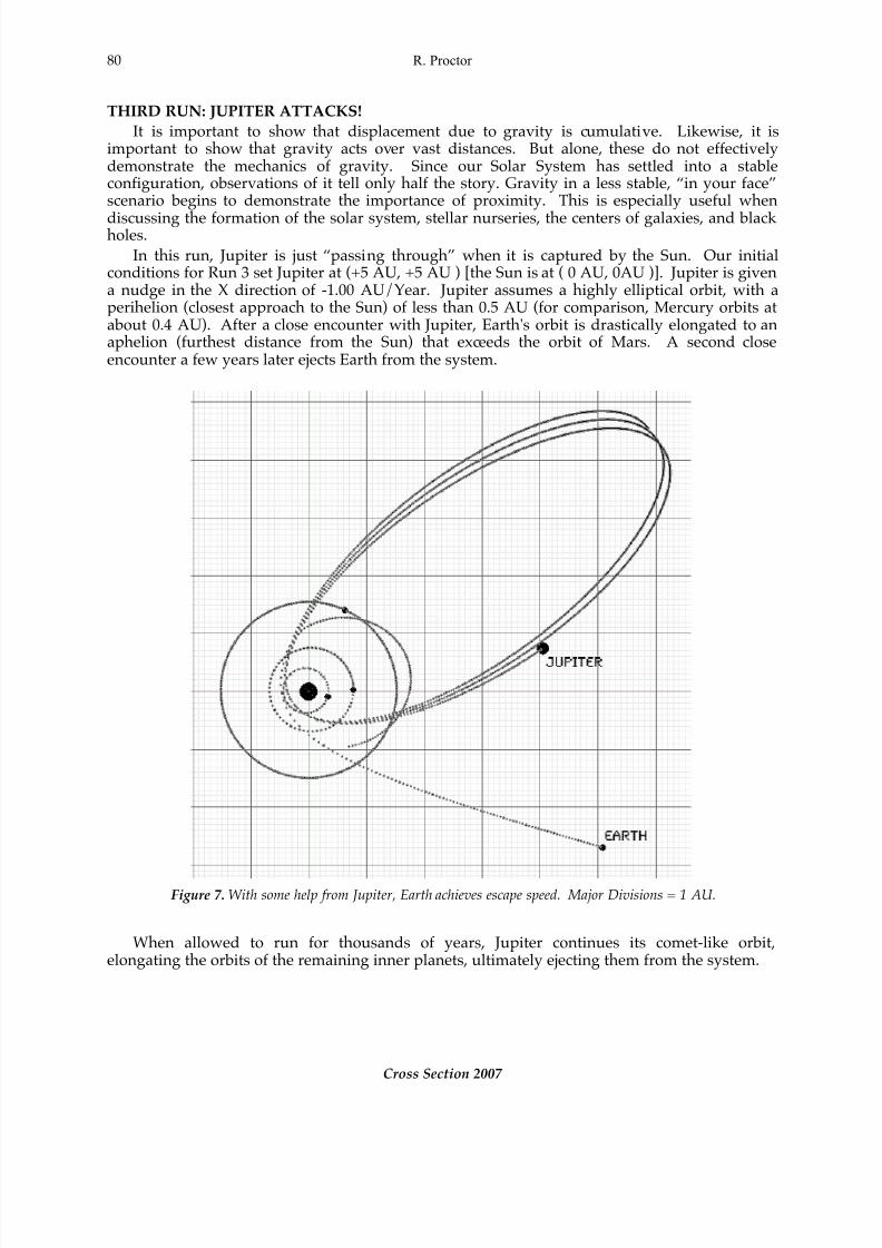
In this run, Jupiter is just “passing through” when it is captured by the Sun. Our initialconditions for Run 3 set Jupiter at (+5 AU, +5 AU ) [the Sun is at ( 0 AU, 0AU )]. Jupiter is givena nudge in the X direction of -1.00 AU/Year. Jupiter assumes a highly elliptical orbit, with aperihelion (closest approach to the Sun) of less than 0.5 AU (for comparison, Mercury orbits atabout 0.4 AU). After a close encounter with Jupiter, Earth's orbit is drastically elongated to anaphelion (furthest distance from the Sun) that exceeds the orbit of Mars. A second closeencounter a few years later ejects Earth from the system.

Figure 7. With some help from Jupiter, Earth achieves escape speed. Major Divisions = 1 AU.

When allowed to run for thousands of years, Jupiter continues its comet-like orbit,elongating the orbits of the remaining inner planets, ultimately ejecting them from the system.





CONCLUSIONS Our code appears to produce a reasonably good approximation of the inner Solar System,

plus Jupiter. We believe that, with further development, this project will be a valuable tool forteaching gravitational interactions on an astronomical scale.

Although it works, the code needs major improvements:

1. The Sun should be affected by the other planets (it is currently static).2. A graphical user interface is needed (currently, users must edit the code).3. Code needs to be optimized to handle n bodies (addition of asteroids, et cetera).4. An adaptive time-step should be introduced to improve calculation accuracy.

From personal experience, we can report that this program is a lot of fun to operate. Thestill images in this paper are nothing compared to seeing it in motion!

REFERENCES

Griffiths, D. V.; Smith, I. M. (1991). Numerical methods for engineers: a programmingapproach. Boca Raton: CRC Press, page 218. ISBN 0-8493-8610-1.

Malmrose, M. (2007). Using Python Scripting in Blender.<http://weber.edu/planetarium/productionshare/production_tools/monty.pdf>Accessed 13 December 2007.

Trundle, K., Atwood, R., & Christopher, J. (2001). Preservice Elementary Teachers'Conceptions of Moon Phases before and After Instruction. Journal of Research in ScienceTeaching, 39, 633-658.



82 R. Proctor

Cross Section 2007

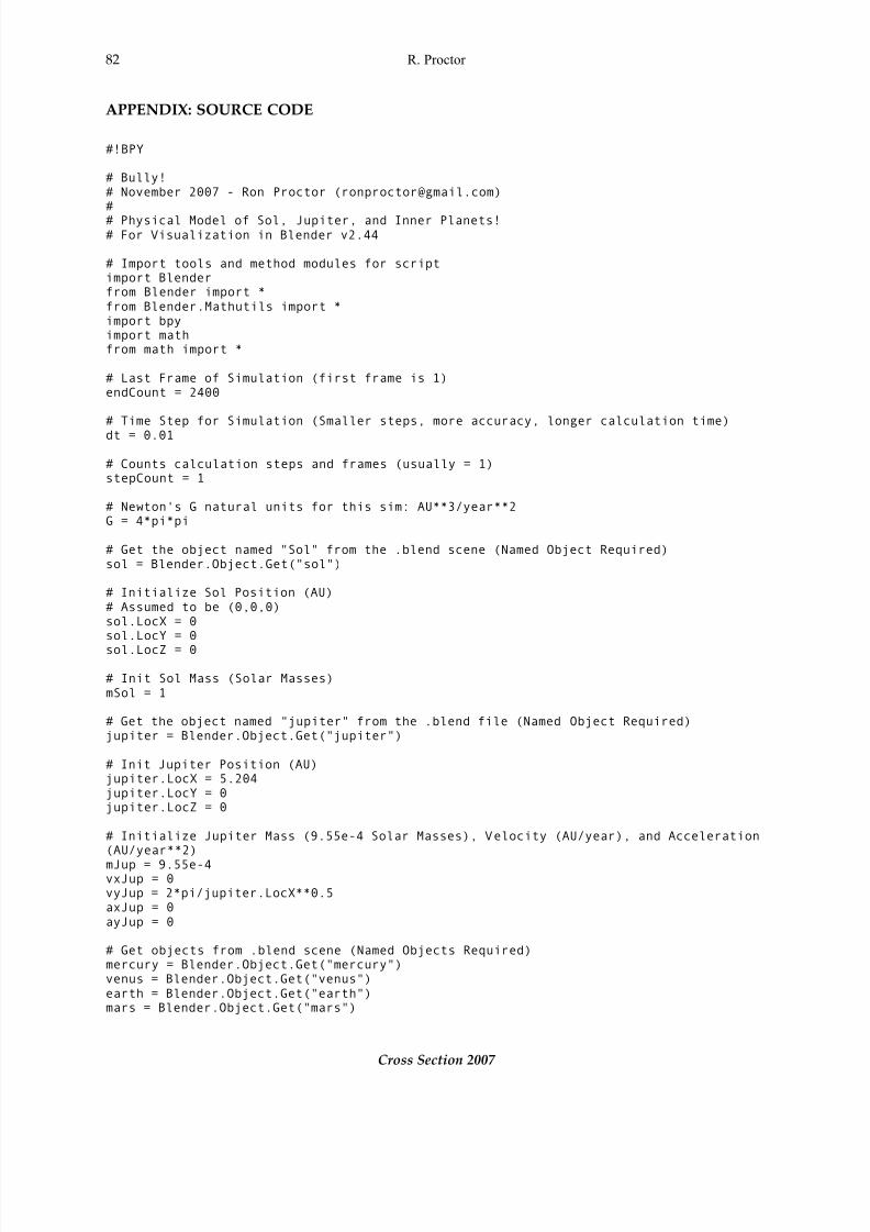
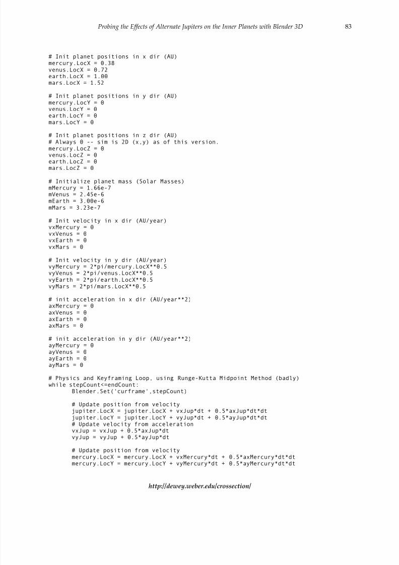
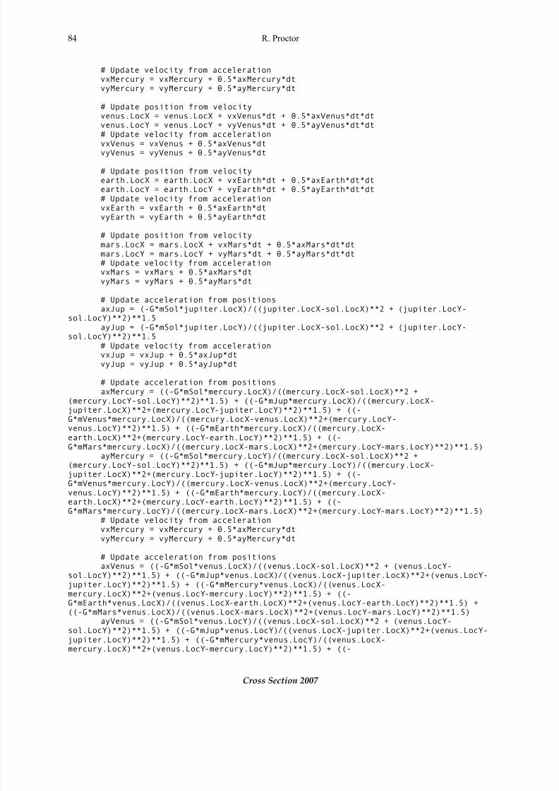
APPENDIX: SOURCE CODE

#!BPY

# Bully!

# November 2007 - Ron Proctor ([email protected])#

# Physical Model of Sol, Jupiter, and Inner Planets!

# For Visualization in Blender v2.44

# Import tools and method modules for scriptimport Blenderfrom Blender import *

from Blender.Mathutils import *

import bpyimport mathfrom math import *

# Last Frame of Simulation (first frame is 1)

endCount = 2400

# Time Step for Simulation (Smaller steps, more accuracy, longer calculation time)

dt = 0.01

# Counts calculation steps and frames (usually = 1)stepCount = 1

# Newton's G natural units for this sim: AU**3/year**2G = 4*pi*pi

# Get the object named "Sol" from the .blend scene (Named Object Required)

sol = Blender.Object.Get("sol")

# Initialize Sol Position (AU)

# Assumed to be (0,0,0)

sol.LocX = 0sol.LocY = 0

sol.LocZ = 0

# Init Sol Mass (Solar Masses)

mSol = 1

# Get the object named "jupiter" from the .blend file (Named Object Required)

jupiter = Blender.Object.Get("jupiter")

# Init Jupiter Position (AU)jupiter.LocX = 5.204

jupiter.LocY = 0jupiter.LocZ = 0

# Initialize Jupiter Mass (9.55e-4 Solar Masses), Velocity (AU/year), and Acceleration(AU/year**2)

mJup = 9.55e-4vxJup = 0vyJup = 2*pi/jupiter.LocX**0.5

axJup = 0

ayJup = 0

# Get objects from .blend scene (Named Objects Required)mercury = Blender.Object.Get("mercury")

venus = Blender.Object.Get("venus")

earth = Blender.Object.Get("earth")mars = Blender.Object.Get("mars")



84 R. Proctor

Cross Section 2007

# Update velocity from accelerationvxMercury = vxMercury + 0.5*axMercury*dt

vyMercury = vyMercury + 0.5*ayMercury*dt

# Update position from velocityvenus.LocX = venus.LocX + vxVenus*dt + 0.5*axVenus*dt*dtvenus.LocY = venus.LocY + vyVenus*dt + 0.5*ayVenus*dt*dt

# Update velocity from accelerationvxVenus = vxVenus + 0.5*axVenus*dtvyVenus = vyVenus + 0.5*ayVenus*dt

# Update position from velocityearth.LocX = earth.LocX + vxEarth*dt + 0.5*axEarth*dt*dtearth.LocY = earth.LocY + vyEarth*dt + 0.5*ayEarth*dt*dt

# Update velocity from acceleration

vxEarth = vxEarth + 0.5*axEarth*dtvyEarth = vyEarth + 0.5*ayEarth*dt

# Update position from velocity

mars.LocX = mars.LocX + vxMars*dt + 0.5*axMars*dt*dt

mars.LocY = mars.LocY + vyMars*dt + 0.5*ayMars*dt*dt# Update velocity from accelerationvxMars = vxMars + 0.5*axMars*dt

vyMars = vyMars + 0.5*ayMars*dt

# Update acceleration from positionsaxJup = (-G*mSol*jupiter.LocX)/((jupiter.LocX-sol.LocX)**2 + (jupiter.LocY-

sol.LocY)**2)**1.5

ayJup = (-G*mSol*jupiter.LocY)/((jupiter.LocX-sol.LocX)**2 + (jupiter.LocY-sol.LocY)**2)**1.5

# Update velocity from accelerationvxJup = vxJup + 0.5*axJup*dt

vyJup = vyJup + 0.5*ayJup*dt

# Update acceleration from positions

axMercury = ((-G*mSol*mercury.LocX)/((mercury.LocX-sol.LocX)**2 +

(mercury.LocY-sol.LocY)**2)**1.5) + ((-G*mJup*mercury.LocX)/((mercury.LocX-jupiter.LocX)**2+(mercury.LocY-jupiter.LocY)**2)**1.5) + ((-G*mVenus*mercury.LocX)/((mercury.LocX-venus.LocX)**2+(mercury.LocY-venus.LocY)**2)**1.5) + ((-G*mEarth*mercury.LocX)/((mercury.LocX-

earth.LocX)**2+(mercury.LocY-earth.LocY)**2)**1.5) + ((-

G*mMars*mercury.LocX)/((mercury.LocX-mars.LocX)**2+(mercury.LocY-mars.LocY)**2)**1.5)ayMercury = ((-G*mSol*mercury.LocY)/((mercury.LocX-sol.LocX)**2 +

(mercury.LocY-sol.LocY)**2)**1.5) + ((-G*mJup*mercury.LocY)/((mercury.LocX-

jupiter.LocX)**2+(mercury.LocY-jupiter.LocY)**2)**1.5) + ((-G*mVenus*mercury.LocY)/((mercury.LocX-venus.LocX)**2+(mercury.LocY-

venus.LocY)**2)**1.5) + ((-G*mEarth*mercury.LocY)/((mercury.LocX-earth.LocX)**2+(mercury.LocY-earth.LocY)**2)**1.5) + ((-G*mMars*mercury.LocY)/((mercury.LocX-mars.LocX)**2+(mercury.LocY-mars.LocY)**2)**1.5)

# Update velocity from accelerationvxMercury = vxMercury + 0.5*axMercury*dt

vyMercury = vyMercury + 0.5*ayMercury*dt

# Update acceleration from positionsaxVenus = ((-G*mSol*venus.LocX)/((venus.LocX-sol.LocX)**2 + (venus.LocY-

sol.LocY)**2)**1.5) + ((-G*mJup*venus.LocX)/((venus.LocX-jupiter.LocX)**2+(venus.LocY-

jupiter.LocY)**2)**1.5) + ((-G*mMercury*venus.LocX)/((venus.LocX-

mercury.LocX)**2+(venus.LocY-mercury.LocY)**2)**1.5) + ((-G*mEarth*venus.LocX)/((venus.LocX-earth.LocX)**2+(venus.LocY-earth.LocY)**2)**1.5) +((-G*mMars*venus.LocX)/((venus.LocX-mars.LocX)**2+(venus.LocY-mars.LocY)**2)**1.5)

ayVenus = ((-G*mSol*venus.LocY)/((venus.LocX-sol.LocX)**2 + (venus.LocY-

sol.LocY)**2)**1.5) + ((-G*mJup*venus.LocY)/((venus.LocX-jupiter.LocX)**2+(venus.LocY-

jupiter.LocY)**2)**1.5) + ((-G*mMercury*venus.LocY)/((venus.LocX-mercury.LocX)**2+(venus.LocY-mercury.LocY)**2)**1.5) + ((-





G*mEarth*venus.LocY)/((venus.LocX-earth.LocX)**2+(venus.LocY-earth.LocY)**2)**1.5) +((-G*mMars*venus.LocY)/((venus.LocX-mars.LocX)**2+(venus.LocY-mars.LocY)**2)**1.5)


vxVenus = vxVenus + 0.5*axVenus*dtvyVenus = vyVenus + 0.5*ayVenus*dt


axEarth = ((-G*mSol*earth.LocX)/((earth.LocX-sol.LocX)**2 + (earth.LocY-sol.LocY)**2)**1.5) + ((-G*mJup*earth.LocX)/((earth.LocX-jupiter.LocX)**2+(earth.LocY-jupiter.LocY)**2)**1.5) + ((-G*mMercury*earth.LocX)/((earth.LocX-mercury.LocX)**2+(earth.LocY-mercury.LocY)**2)**1.5) + ((-

G*mVenus*earth.LocX)/((earth.LocX-venus.LocX)**2+(earth.LocY-venus.LocY)**2)**1.5) +((-G*mMars*earth.LocX)/((earth.LocX-mars.LocX)**2+(earth.LocY-mars.LocY)**2)**1.5)

ayEarth = ((-G*mSol*earth.LocY)/((earth.LocX-sol.LocX)**2 + (earth.LocY-

sol.LocY)**2)**1.5) + ((-G*mJup*earth.LocY)/((earth.LocX-jupiter.LocX)**2+(earth.LocY-

jupiter.LocY)**2)**1.5) + ((-G*mMercury*earth.LocY)/((earth.LocX-mercury.LocX)**2+(earth.LocY-mercury.LocY)**2)**1.5) + ((-G*mVenus*earth.LocY)/((earth.LocX-venus.LocX)**2+(earth.LocY-venus.LocY)**2)**1.5) +((-G*mMars*earth.LocY)/((earth.LocX-mars.LocX)**2+(earth.LocY-mars.LocY)**2)**1.5)


vxEarth = vxEarth + 0.5*axEarth*dtvyEarth = vyEarth + 0.5*ayEarth*dt


axMars = ((-G*mSol*mars.LocX)/((mars.LocX-sol.LocX)**2 + (mars.LocY-sol.LocY)**2)**1.5) + ((-G*mJup*mars.LocX)/((mars.LocX-jupiter.LocX)**2+(mars.LocY-jupiter.LocY)**2)**1.5) + ((-G*mMercury*mars.LocX)/((mars.LocX-mercury.LocX)**2+(mars.LocY-mercury.LocY)**2)**1.5) + ((-

G*mEarth*mars.LocX)/((mars.LocX-earth.LocX)**2+(mars.LocY-earth.LocY)**2)**1.5) + ((-G*mEarth*mars.LocX)/((mars.LocX-earth.LocX)**2+(mars.LocY-earth.LocY)**2)**1.5)

ayMars = ((-G*mSol*mars.LocY)/((mars.LocX-sol.LocX)**2 + (mars.LocY-sol.LocY)**2)**1.5) + ((-G*mJup*mars.LocY)/((mars.LocX-jupiter.LocX)**2+(mars.LocY-

jupiter.LocY)**2)**1.5) + ((-G*mMercury*mars.LocY)/((mars.LocX-mercury.LocX)**2+(mars.LocY-mercury.LocY)**2)**1.5) + ((-G*mEarth*mars.LocY)/((mars.LocX-earth.LocX)**2+(mars.LocY-earth.LocY)**2)**1.5) + ((-

G*mEarth*mars.LocY)/((mars.LocX-earth.LocX)**2+(mars.LocY-earth.LocY)**2)**1.5)

# Update velocity from accelerationvxMars = vxMars + 0.5*axMars*dtvyMars = vyMars + 0.5*ayMars*dt

mercury.insertIpoKey(3)

venus.insertIpoKey(3)earth.insertIpoKey(3)mars.insertIpoKey(3)

jupiter.insertIpoKey(3)

# Redraw 3D WindowBlender.Redraw()

# advance stepCountstepCount = stepCount+1

# Loop from "while..." until endCount is reached.

# It's Over!

tecnical animation

Documents