SUPPLEMENTARY INFORMATION

Negative biotic interactions drive predictions of

distributions for species from a grassland community

Phillip P.A. Staniczenko1,2,†, K. Blake Suttle3 & Richard G. Pearson4

1National Socio-Environmental Synthesis Center (SESYNC), MD, USA2Department of Biology, University of Maryland College Park, MD, USA

3Department of Ecology and Evolutionary Biology, UC Santa Cruz, CA, USA4Centre for Biodiversity and Environment Research, University College London, UK

†Present address: Department of Biology, Brooklyn College, City University of New York, NY, USA

Author for correspondence: Phillip P.A. Staniczenko, pstaniczenko@brooklyn.cuny.edu

This document contains additional description of materials and methods in two

sections: (i) Species distribution models for the California grassland community,

and (ii) Measuring data compression using Bayesian networks and total length.

1

Species distribution models for the California grassland community

We implemented species distribution models (SDMs) in R using the BIOMOD platform

(Thuiller et al. 2009). The species pool contained 53 plant and 1 grasshopper species (Ta-

ble S1) found at the Angelo Coast Range Reserve (39◦ 44′ 17.7′′ N, 123◦ 37′ 48.4′′ W), a

protected and relatively undisturbed area of 7,660 acres in northern California. We down-

loaded presence records for these species from the Global Biodiversity Information Facility

(http://GBIF.org), and, for each species, we classified as “present” any 800m× 800m grid

cell in the western USA (32◦ N to 49.1◦ N and 125◦ W to 115◦ W) that contained one or

more presence records.

For both prior and posterior community distribution matrices, we used the Maxent

method (Elith et al. 2011) to estimate species’ responses to bioclimate variables. Following

Fithian & Hastie (2013), consider predicting the distribution of an individual species across

a geographical domain D at locations z ∈ D. Associated with each location is a vector

of measured bioclimate variables or features x(z). A presence-only data set consists of n1

locations of species sightings zk ∈ D for k = 1, 2, . . . , n1, and n0 “background” locations zk for

k = n1 +1, 2, . . . , n1 +n0; and let xk = x(zk) be the features for location k. The suitability of

a location for the species is given by N(zk) ∼ Poisson(λ(zk)); where the intensity is log-linear

in features x(z):

λ(z) = eα+βx(z) (S1)

Notice that α only multiplies λ(z) by a constant, so β completely determines the distribution

of habitat suitability across the geographical domain: pλ(z) = eβx(z)∫D eβx(z)dz

. Computing the

maximum entropy solution is equivalent to computing the maximum likelihood for Eqn (S1)

given sighting data. There are two steps: i) Obtain the maximum likelihood estimate density

pλ(z), which requires finding β for which the density is “nearly geographically uniform” (i.e.,

2

entropy is maximised) subject to constraints that make it resemble the sighting data; and

ii) Multiply pλ(z) by n1, which requires finding α such that λ(z) = n1pλ(z). In practice, we

used Maxent’s logistic output in BIOMOD to obtain prior habitat suitability values (ranging

from 0 to 1) at each location.

We considered seven bioclimate variables: maximum temperature of the warmest month;

minimum temperature of the coldest month; annual precipitation; precipitation of the dri-

est quarter; mean temperature of the wettest quarter; temperature seasonality (standard

deviation × 100); and precipitation seasonality (coefficient of variation). The climate vari-

ables were derived from an ensemble of five atmosphere-ocean general circulation models

for the year 2010, and are freely available online (Pearson et al. 2014; http://dx.doi.org/

10.7917/D7WD3XH5). For reference, climate variables at Angelo Coast Range Reserve are

provided in Table S2.

For the posterior community distribution matrix, we modelled the effects of biotic inter-

actions, shared habitat suitability, and other interspecific relationships on range predictions

for 14 focal species using a method that also uses Bayesian networks (BNs; Staniczenko et al.

2017). The California grassland BN contains a total of 52 conditional dependencies, repre-

senting 6 positive and 9 negative biotic interactions, 32 positive shared habitat suitability

relationships, and 2 positive and 3 negative uncategorised interspecific relationships; these

interspecific relationships were classified according to a series of transplant and competitor-

removal experiments (Thomsen et al. 2006; Suttle & Thomsen 2007), consumer addition

and removal experiments (Suttle et al. 2007), and long-term monitoring studies (Sullivan

et al. 2016). In practice, conditional dependencies modify prior habitat suitability values

to produce posterior habitat suitability values that also include the effects of interspecific

relationships; as with our prior habitat suitability values, posterior habitat suitability values

3

also range from 0 to 1. Because prior habitat suitability values for non-focal species were, by

design, unchanged by the California grassland BN, we only considered the 14 focal species

in subsequent analysis.

Given a set of prior habitat suitability values for the 14 focal species and a corresponding

set of posterior habitat suitability values, we converted habitat suitability values for each

species in each matrix to a binary range using one of two threshold rules. For example,

with the maxSens threshold, we considered each species in turn and identified the habitat

suitability value that would result in all recorded presences (species sightings) being included

in its estimated range; that is, all habitat suitability values above the threshold value were

assigned “1” and all habitat suitability values below the threshold value were assigned “0”. A

similar process was used for the maxSSS threshold, but a different, typically larger threshold

habitat suitability value was identified for each species and each matrix. The resulting prior

and posterior community distribution matrices describe binary range predictions for multiple

species (columns) at distinct locations (rows), and are suitable for data compression analysis

to determine which interspecific relationships drive predictions of species’ distributions.

Measuring data compression using Bayesian networks and total

length

In data compression analysis, we represent interspecific relationships by conditional depen-

dencies in a BN model. Whereas in the above section we used BNs to modify prior habitat

suitability values to generate posterior habitat suitability values, we now use BNs to assess

the strength of similarity or difference between range predictions in a community distribution

matrix. For example, consider the BN model in Fig. 1 of the main text, which represents

three species and one positive and one negative interspecific relationship by three nodes and

4

one positive and one negative conditional dependency: A → C and B 6→ C. Rather than

prescribing a rule that increases the habitat suitability value of C if A is likely to be present

at a particular location and decreasing the habitat suitability value of C if B is likely to be

present at a particular location, in this application we use the BN as a compression model

to test if the predicted ranges of species A and B contain meaningful information about the

predicted range of species C.

In this example, we do not need to consider state tables (also known as conditional

probability tables) for species A and B for data compression analysis because their binary

ranges are not affected by interspecific relationships—in SDMs, at least—and are therefore

the same in both prior and posterior community distribution matrices. The state table for

species C is

A B C1 1 pC,31 0 pC,20 1 pC,10 0 pC,0

where there is a distinct probability for each unique state of A and B. We would expect

pC,2 to have the highest value given the assumption of a positive conditional dependency

between A and C, pC,1 to have the lowest value given the assumption of a negative conditional

dependency between B and C, and intermediate values for pC,0 and pC,3 (whether pC,0 ≥ pC,3

or pC,0 ≤ pC,3 would be determined by how A and B combine to affect C).

Maximum likelihood probabilities are calculated from data, in this case community dis-

tribution matrices, and for data compression analysis their relative values are less important

than the requirement that each state has a distinct probability (the is equivalent to the

“FULL” model described in Staniczenko et al. 2017). This requirement ensures that total

5

lengths, which are calculated from maximum likelihood probabilities, reflect not only the

effects of each interspecific relationship on range predictions, but also the effects of each

combination of interspecific relationships on range predictions.

Total length can be calculated as the log2-transformed version of normalized maximum

likelihood (NML; Rissanen 2001; Myung et al. 2006; Staniczenko et al. 2014). In this study,

NML quantifies how well a BN model representing interspecific relationships explains a par-

ticular community distribution matrix compared to how well the model explains all possible

community distribution matrices with the same number of species and locations. A good

model explains only the focal community distribution matrix well and all other matrices

poorly, resulting in high NML and short total length. By contrast, an overly simplistic

model is likely to explain the focal matrix no better than it does any other matrix, resulting

in low NML and long total length. And although an overly complex model is likely to explain

the focal matrix well, it will also explain all other matrices well due to its greater inherent

flexibility, still resulting in low NML and short total length.

For BN model M and community distribution matrix B, NML can be written as

NML(M |B) =L(M, ~pB|B)∑B′ L(M, ~pB′ |B

′)(S2)

where L is a likelihood function and ~pB is a vector of maximum likelihood probabilities

from state tables associated with M . In Eqn (S2), conventional likelihood is normalised

over all matrices B′ with the same number of rows and columns as the original community

distribution matrix B.

6

For binary matrices, each element can be considered the outcome of a Bernoulli trial

and so the maximum likelihood estimate of state table probability pl is

pl =Ul

Ul + Zl(S3)

where Ul is the number of ones (locations within a predicted range) and Zl the number of

zeros (locations outside a predicted range) in B that are associated with pl. For example,

consider the state table for species C, and, in particular, the case in which the predicted

ranges of species A and B overlap, which has an associated probability pC,3. Imagine that

a corresponding community distribution matrix has 20 rows (locations) and the predicted

ranges of A and B overlap at 6 locations. If the predicted range of C includes 4 of these 6

locations then pC,3 = 4/(4 + 2) = 2/3. Similar calculations involving sections of the other 14

rows (e.g., locations in which the predicted ranges of A and B do not overlap for pC,0) would

give maximum likelihood estimates for the three remaining state table probabilities.

The maximum likelihood function for binary matrices is

L(M, ~pB|B) =∏l

pUll (1− pl)Zl (S4)

where the product is taken over the complete set of state table probabilities in ~pB.

7

Total length, as the log2-transformed version of NML, is

LM(B) = − log2 NML(M |B)

= − log2 L(M, ~pB|B) + log2

∑B′L(M, ~pB′ |B′)

= − log2 L(M, ~pB|B) + log2 C(M,B)

(S5)

where C(M,B) is a penalisation constant known as the parametric complexity or regret (Ris-

sanen 1986, 1987, 1989, 1996).

Parametric complexity has a surprisingly simple form when model parameters are condi-

tionally independent (Staniczenko et al. 2014)1. However, calculating parametric complexity

is less straightforward with BN models due to conditional dependencies between random vari-

ables (Grunwald 2007). One solution is factorised NML (fNML), which has been shown to

provide a good approximation to NML (Silander et al. 2008, 2009). For BN models, fNML

involves calculating NML for each matrix column separately and multiplying the results. In

practice, Eqn (S5) is applied to each matrix column and corresponding state table in turn,

and component total lengths are summed to give a final total length.

1Parametric complexity can be decomposed into separate contributions for each state table probabilityin the model. Writing Xl = Ul + Zl, the denominator in Eqn (S2) becomes

∑B′

L(M, ~pB′ |B′) =

∑l

L(M, pl|B′) =

∏l

Xl∑k=0

(Xl

k

)(k

Xl

)k (Xl − kXl

)(Xl−k)

=∏l

C(Xl) (S6)

with the contribution for each state table probability pl written as

C(Xl) = 1 +eXlΓ(Xl, Xl)

XXl−1l

≈ 1 +

(√Xlπ

2− 1

3+

√2π

24√Xl

− 4

135Xl+

√2π

576√X3

l

+8

2835X2l

)(S7)

which can be computed quickly (Staniczenko et al. 2014).

8

Because absolute changes in total length can be unwieldy when a community distri-

bution matrix contains a large number of locations, it is clearer to present values scaled

by the number of bits required to transmit an uncompressed version of the matrix. With

binary matrices, this reference total length is simply the number of matrix rows (locations)

multiplied by the number of matrix columns (species).

Implications of the requirement that Bayesian networks are acyclic for mod-

elling interspecific relationships in species distribution models

The requirement that a Bayesian network is acyclic restricts how the effect of an interspecific

relationship can be modelled in our approach, particularly when the effects of an interaction

could be symmetric (e.g., mutualistic or competitive interactions). In the case of competition,

the main consideration is that one species must be identified as the stronger of the two

competitors, with the stronger competitor influencing the occurrence probability (or habitat

suitability value) of the weaker competitor. Once the direction of influence has been defined,

a high occurrence probability (or habitat suitability value) for the stronger competitor is

modelled as reducing the occurrence probability (or habitat suitability value) for the weaker

competitor compared to its environment-only probability. Clearly, this imposed asymmetry

is more realistic when interaction strengths are unequal between species and less realistic

when strengths are more equal. Finally, it is worth noting that modelling an interaction

in this way has no effect on the stronger competitor—due to the uni-directionality of a

conditional dependency, only the estimated range of the weaker competitor is considered in

data compression analysis.

9

Implications of the requirement that Bayesian networks are acyclic for com-

paring the effect of interspecific relationships on community distributions

We tested the sensitivity of our results to the directionality of interspecific relationships in

compression models by repeating analyses with a new set of Bayesian networks in which the

sign of interspecific relationships is maintained from corresponding original versions but the

direction of influence is reversed. We considered the same prior and posterior community

distribution matrices with a new set of eight compression models: ALL reverse, SHS BI

reverse, SHS BI+ reverse, SHS BI– reverse, SHS reverse, BI reverse, BI+ reverse, BI– reverse.

It is first important to note that it is not informative to compare raw values of ∆M and

∆%M between the set of original compression models and the set of corresponding “reverse”

models. This is because different numbers of species are potentially affected and so the

scaling constant is different between the two sets of models, i.e., 13 focal species are assessed

for compression with ALL (1 of the 14 focal species has no conditional dependencies), in

comparison to 7 focal species and 23 non-focal species with ALL reverse. However, it is

informative to compare differences in model rankings between the set of original compression

models and the set of “reverse” compression models.

Rankings are similar between the two sets of compression models (Table S3). With the

maxSSS threshold, the ranking for ∆M among “reverse” Bayesian network models is exactly

the same as with original models; rankings are similar for ∆%M, with BI– and BI– reverse

top-ranked in their respective model sets. With the maxSens threshold, rankings are similar

for ∆M, and BI– and BI– reverse are again top-ranked in their respective model sets for

10

∆%M. These findings show that our approach, results, and conclusions are insensitive to

directionality in Bayesian network compression models, especially when using the maxSSS

threshold and when considering model rankings for ∆%M. (Of course, directionality is im-

portant when modelling interspecific relationships in species distribution models, such that

range predictions are modified for the intended species.)

Results for alternative Bayesian networks for modifying habitat suitability val-

ues in species distribution models

We repeated our workflow with two alternative Bayesian networks for modifying habitat

suitability values in SDMs (see Fig. 1 in main text): (i) only shared habitat suitability rela-

tionships (32 positive conditional dependencies) and (ii) only biotic interactions (6 positive

and 9 negative conditional dependencies). With only shared habitat suitability relationships

in SDMs, we would expect, of our eight compression models (ALL, SHS BI, SHS BI+, SHS

BI–, SHS, BI, BI+, BI–; see Fig. 2 in main text), BI, BI+, and BI– to perform worse than

compression models that include SHS because those interactions are not included in the

SDMs. By contrast, with only biotic interactions in SDMs, we would expect BI, BI+, and

BI– to perform better than compression models that include SHS.

We have already established that modelling 52 interspecific relationships between species

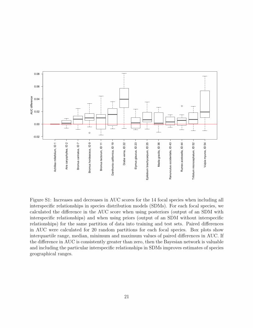
from the California grassland community using a Bayesian network improves range predic-

tions for 13 focal species, with model performance measured as increases in AUC compared to

when no interspecific relationships are modelled in SDMs (Staniczenko et al. 2017; Fig. S1).

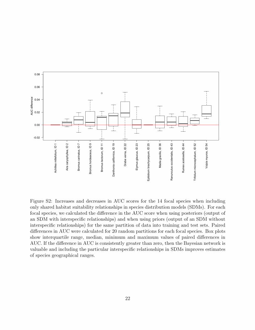
Model performance is still good for the two alternative Bayesian networks with only shared

11

habitat suitability relationships (Fig. S2) and only biotic interactions (Fig. S3), although

understandably fewer predicted ranges are modified.

With only shared habitat suitability relationships in SDMs, results for the maxSens

threshold show that the SHS compression model moves from being lowly ranked (when all

52 interspecific relationships are modelled) to top-ranked while BI, BI+, and BI– move from

highly ranked to bottom-ranked, as expected (for both ∆M and ∆%M; Table S4). Similarly,

results for the maxSSS threshold show that all compression models that include SHS rank

higher than BI, BI+, and BI–.

With only biotic interactions in SDMs, results for the maxSens threshold show that BI,

BI+, and BI– remain top-ranked (compared to when all 52 interspecific relationships are

modelled) and the order remains BI– then BI then BI+ (for both ∆M and ∆%M). Results

for maxSSS and ∆M show that BI, BI+, and BI– move from bottom-ranked to top-ranked.

Interestingly, although results for maxSSS and ∆%M show that BI and BI+ move from lowly

ranked to highly ranked, as expected, BI– moves from top-ranked to bottom-ranked.

The finding that BI– drops in ranking when modelling only biotic interactions in SDMs

suggests that modelling negative biotic interactions is most important when the two species

involved in the interaction are likely to occur together in the absence of other species that

may influence the presence of the focal species. One can understand this interpretation as

follows. With our current implementation of modelling interspecific relationships in SDMs,

the effect of negative biotic interactions is very strong in the absence of positive shared habi-

tat suitability relationships. That is, modelled negative biotic interactions reduce habitat

12

suitability values (HSVs) of affected species more often and by greater amounts than they

otherwise would if all interspecific relationships were to be modelled. Because HSVs are sys-

tematically lower when mainly negative biotic interactions are modelled in SDMs, maxSSS

“overcorrects” when transforming HSVs to a binary presence-absence range, and in doing

so dilutes the effect of modelling negative biotic interactions in SDMs. This dilution effect

explains why BI– does not lead to as much compression when modelling only biotic inter-

actions in SDMs compared to modelling all interspecific relationships. (Note that maxSens

does not appear to result in this dilution effect.)

To illustrate this dilution effect, consider a focal species A that is negatively influenced

by a biotic interaction with species B and positively influenced by a shared habitat suit-

ability relationship (or some other positive interspecific relationship) with species C. First

consider the case in which both negative and positive interspecific relationships are mod-

elled in the SDM for species A. When all three species are likely to occur together based

on an environment-only SDM—i.e., all three species have high prior HSVs at a particular

location—then the effects of the positive and negative interspecific relationship are modelled

as cancelling one another out. When only species A and B are likely to occur together,

the negative biotic interaction has a large effect on the posterior HSV of species A, which is

picked up by the BI– compression model. By contrast, consider the case in which the positive

interspecific relationship between species A and C is not modelled in the SDM for species A.

The negative biotic interaction between species A and B “incorrectly” reduces the posterior

HSV of species A when all three species are likely to occur together. Subsequently, maxSSS

13

“overcorrects” and identifies a threshold HSV for species A that is very different from both

the threshold value for prior HSVs and posterior HSVs when all interspecific relationships

are modelled in the SDM for species A. This overcorrection leads to a dilution of the effect of

negative biotic interactions on the predicted range of species A when only biotic interactions

are modelled in SDMs, and therefore gives rise to the result that BI– performs less well as a

compression model.

References

Ehrlen, J. & Morris, W.F. (2015). Predicting changes in the distribution and abundance of

species under environmental change. Ecol. Lett., 18, 303–314.

Elith, J., Phillips, S.J., Hastie, T., Dudık, M., Chee, Y.E. & Yates, C.J. (2011). A statistical

explanation of MaxEnt for ecologists. Divers. Distrib., 17, 43–57.

Fithian, W. & Hastie, T. (2013). Finite-sample equivalence in statistical models for presence-

only data. Ann. Appl. Stat., 7, 1917–1939.

Grunwald, P.D. (2007). The Minimum Description Length Principle. MIT Press.

Myung, J.I., Navarro, D.J. & Pitt, M.A. (2006). Model selection by normalized maximum

likelihood. J. Math. Psychol., 50, 167–179.

Pearson, R.G. et al. (2014). Life history and spatial traits predict extinction risk due to

climate change. Nat. Clim. Change, 4, 217–221.

Rissanen, J. (1986). Stochastic complexity and modeling. Ann. Stat., 14, 1080–1100.

Rissanen, J. (1987). Stochastic complexity. J. R. Stat. Soc. B, 49, 223–239.

Rissanen, J. (1989). Stochastic Complexity in Statistical Inquiry. World Scientific Publishing.

Rissanen, J. (1996). Fisher information and stochastic complexity. IEEE Trans. Inf. Theory,

42, 40–47.

14

Rissanen, J. (2001). Strong optimality of the normalized ML models as universal codes and

information in data. IEEE Trans. Inf. Theory, 47, 1712–1717.

Silander, T., Roos, T., Kontkanen, P. & Myllymaki, P (2008). Factorized normalized maxi-

mum likelihood criterion for learning Bayesian network structures. In: Proceedings of the

4th European workshop on probabilistic graphical models (PGM-08).

Silander, T., Roos, T. & Myllymaki, P (2009). Locally minimax optimal predictive modeling

with Bayesian networks. In: Proceedings of the 12th International Conference on Artificial

Intelligence and Statistics (AISTATS-09).

Staniczenko, P.P.A, Sivasubramaniam, P., Suttle, K.B. & Pearson, R.G. (2017). Linking

macroecology and community ecology: Refining predictions of species distributions using

biotic interaction networks. Ecol. Lett., 20, 693–707.

Staniczenko, P.P.A., Smith, M.J. & Allesina, S. (2014). Selecting food web models using

normalized maximum likelihood. Methods Ecol. Evol., 5, 551–562.

Sullivan, M.J.P., Thomsen, M. & Suttle, K.B. (2016). Grassland responses to increased

rainfall depend on the timescale of forcing. Glob. Change Biol., 22, 1655–1665.

Suttle, K.B. & Thomsen, M. (2007). Climate change and grassland restoration in California:

lessons from six years of rainfall manipulation in a north coast grassland. Madrono, 54,

225–233.

Suttle, K.B., Thomsen, M.A. & Power, M.E. (2007). Species interactions reverse grassland

responses to changing climate. Science, 315, 640–642.

Thomsen, M., D’Antonio, C., Suttle, K.B. & Sousa, W.P. (2006). Ecological resistance,

seed density, and their interaction determine patterns of invasion in a California coastal

grassland. Ecol. Lett., 9, 160–170.

Thuiller, W., Lafourcade, B., Engler, R. & Araujo, M.B. (2009). BIOMOD – a platform for

ensemble forecasting of species distributions. Ecography, 32, 369–373.

15

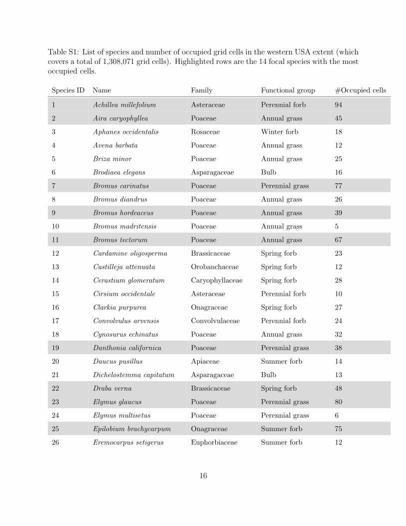
Table S1: List of species and number of occupied grid cells in the western USA extent (whichcovers a total of 1,308,071 grid cells). Highlighted rows are the 14 focal species with the mostoccupied cells.

Species ID Name Family Functional group #Occupied cells

1 Achillea millefolium Asteraceae Perennial forb 94

2 Aira caryophyllea Poaceae Annual grass 45

3 Aphanes occidentalis Rosaceae Winter forb 18

4 Avena barbata Poaceae Annual grass 12

5 Briza minor Poaceae Annual grass 25

6 Brodiaea elegans Asparagaceae Bulb 16

7 Bromus carinatus Poaceae Perennial grass 77

8 Bromus diandrus Poaceae Annual grass 26

9 Bromus hordeaceus Poaceae Annual grass 39

10 Bromus madritensis Poaceae Annual grass 5

11 Bromus tectorum Poaceae Annual grass 67

12 Cardamine oligosperma Brassicaceae Spring forb 23

13 Castilleja attenuata Orobanchaceae Spring forb 12

14 Cerastium glomeratum Caryophyllaceae Spring forb 28

15 Cirsium occidentale Asteraceae Perennial forb 10

16 Clarkia purpurea Onagraceae Spring forb 27

17 Convolvulus arvensis Convolvulaceae Perennial forb 24

18 Cynosurus echinatus Poaceae Annual grass 32

19 Danthonia californica Poaceae Perennial grass 38

20 Daucus pusillus Apiaceae Summer forb 14

21 Dichelostemma capitatum Asparagaceae Bulb 13

22 Draba verna Brassicaceae Spring forb 48

23 Elymus glaucus Poaceae Perennial grass 80

24 Elymus multisetus Poaceae Perennial grass 6

25 Epilobium brachycarpum Onagraceae Summer forb 75

26 Eremocarpus setigerus Euphorbiaceae Summer forb 12

16

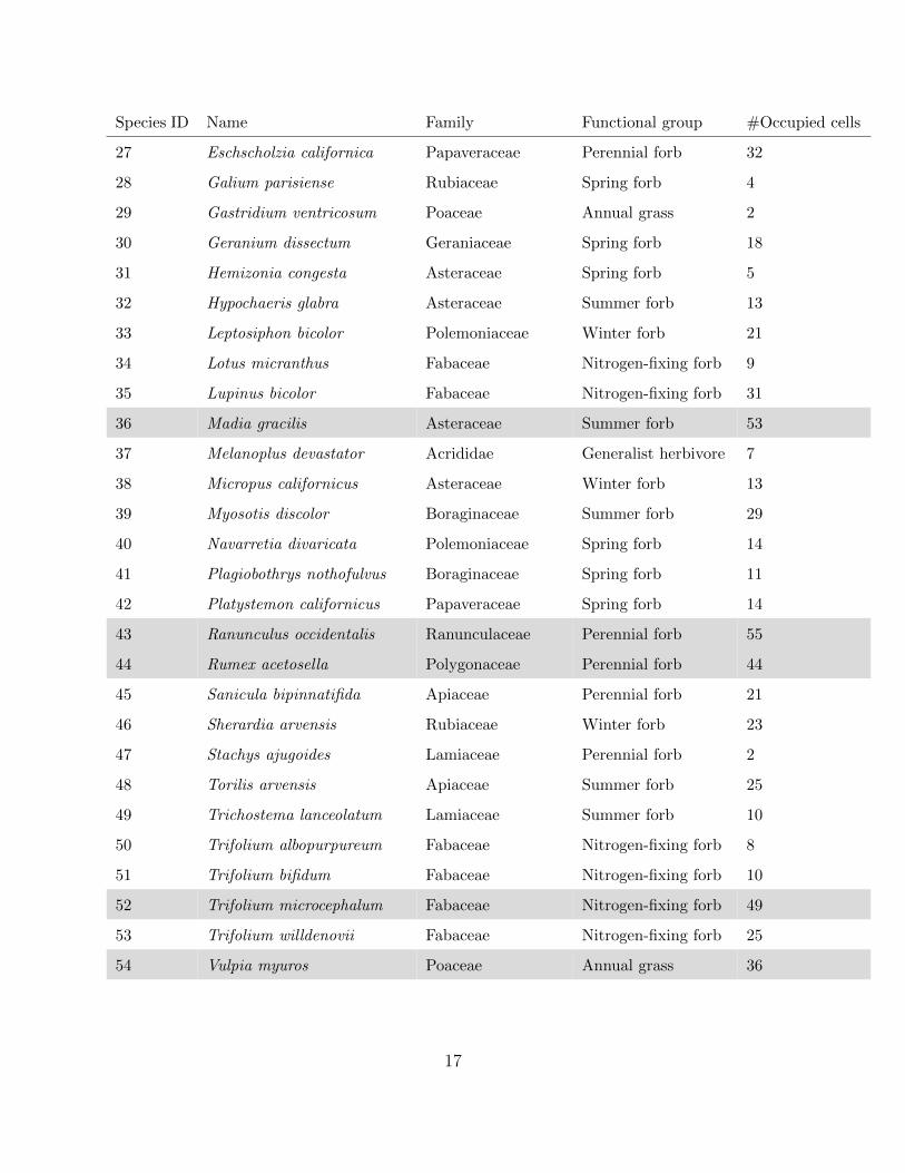
Species ID Name Family Functional group #Occupied cells

27 Eschscholzia californica Papaveraceae Perennial forb 32

28 Galium parisiense Rubiaceae Spring forb 4

29 Gastridium ventricosum Poaceae Annual grass 2

30 Geranium dissectum Geraniaceae Spring forb 18

31 Hemizonia congesta Asteraceae Spring forb 5

32 Hypochaeris glabra Asteraceae Summer forb 13

33 Leptosiphon bicolor Polemoniaceae Winter forb 21

34 Lotus micranthus Fabaceae Nitrogen-fixing forb 9

35 Lupinus bicolor Fabaceae Nitrogen-fixing forb 31

36 Madia gracilis Asteraceae Summer forb 53

37 Melanoplus devastator Acrididae Generalist herbivore 7

38 Micropus californicus Asteraceae Winter forb 13

39 Myosotis discolor Boraginaceae Summer forb 29

40 Navarretia divaricata Polemoniaceae Spring forb 14

41 Plagiobothrys nothofulvus Boraginaceae Spring forb 11

42 Platystemon californicus Papaveraceae Spring forb 14

43 Ranunculus occidentalis Ranunculaceae Perennial forb 55

44 Rumex acetosella Polygonaceae Perennial forb 44

45 Sanicula bipinnatifida Apiaceae Perennial forb 21

46 Sherardia arvensis Rubiaceae Winter forb 23

47 Stachys ajugoides Lamiaceae Perennial forb 2

48 Torilis arvensis Apiaceae Summer forb 25

49 Trichostema lanceolatum Lamiaceae Summer forb 10

50 Trifolium albopurpureum Fabaceae Nitrogen-fixing forb 8

51 Trifolium bifidum Fabaceae Nitrogen-fixing forb 10

52 Trifolium microcephalum Fabaceae Nitrogen-fixing forb 49

53 Trifolium willdenovii Fabaceae Nitrogen-fixing forb 25

54 Vulpia myuros Poaceae Annual grass 36

17

Table S2: Climate variables at the Angelo Coast Range Reserve, California (39◦ 44′ 17.7′′ N,123◦ 37′ 48.4′′ W).

Climate variable 2010

Maximum temperature of the warmest month 27.56◦C

Minimum temperature of the coldest month 2.10◦C

Annual precipitation 2036.41mm

Precipitation of the driest quarter 36.47mm

Mean temperature of the wettest quarter 8◦C

Temperature seasonality (standard deviation × 100) 444

Precipitation seasonality (coefficient of variation) 84

18

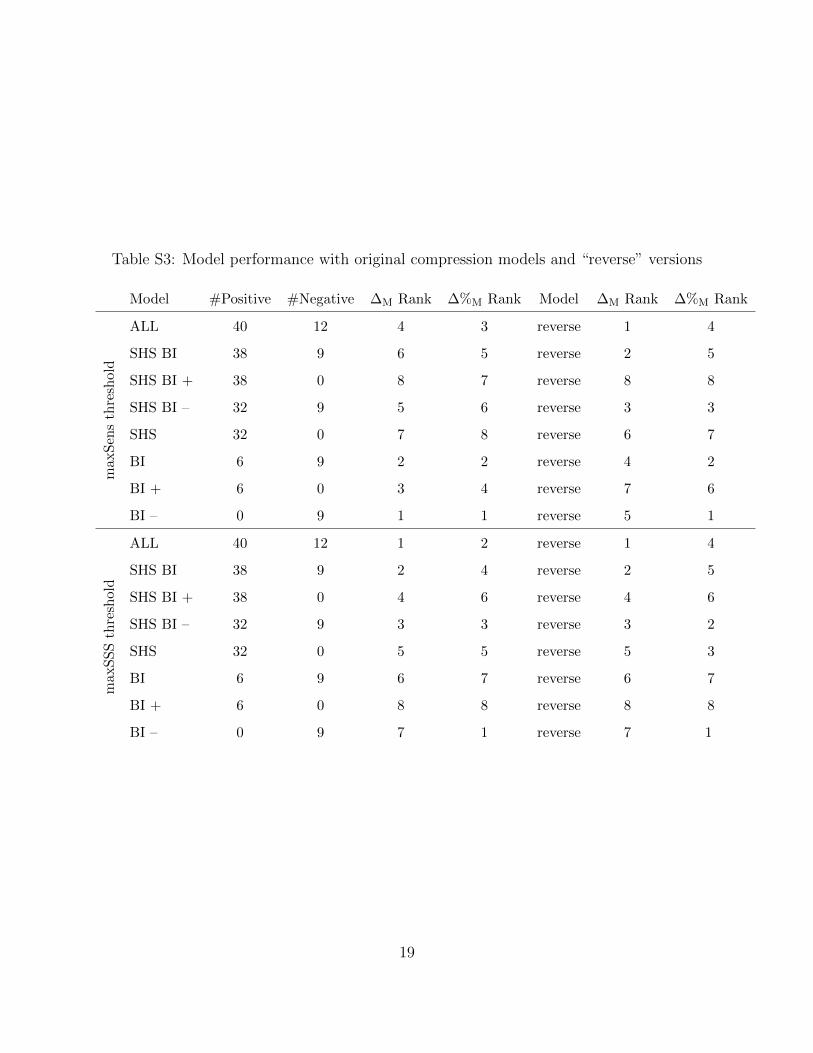
Table S3: Model performance with original compression models and “reverse” versions

Model #Positive #Negative ∆M Rank ∆%M Rank Model ∆M Rank ∆%M Rank

max

Sen

sth

resh

old

ALL 40 12 4 3 reverse 1 4

SHS BI 38 9 6 5 reverse 2 5

SHS BI + 38 0 8 7 reverse 8 8

SHS BI – 32 9 5 6 reverse 3 3

SHS 32 0 7 8 reverse 6 7

BI 6 9 2 2 reverse 4 2

BI + 6 0 3 4 reverse 7 6

BI – 0 9 1 1 reverse 5 1

max

SS

Sth

resh

old

ALL 40 12 1 2 reverse 1 4

SHS BI 38 9 2 4 reverse 2 5

SHS BI + 38 0 4 6 reverse 4 6

SHS BI – 32 9 3 3 reverse 3 2

SHS 32 0 5 5 reverse 5 3

BI 6 9 6 7 reverse 6 7

BI + 6 0 8 8 reverse 8 8

BI – 0 9 7 1 reverse 7 1

19

Table S4: Model performance when modelling different sets of interspecific relationshipsin species distribution models; absolute and percentage changes in compression and corre-sponding ranking (R) among compression models

All interspecific relationships Only shared habitat suitability Only biotic interactions

Model ∆M R ∆%M R ∆M R ∆%M R ∆M R ∆%M R

max

Sen

sth

resh

old

ALL -0.008 4 -2.8% 3 0.013 5 4.2% 5 -0.013 6 -4.2% 6

SHS BI -0.011 6 -3.8% 5 0.014 4 4.6% 4 -0.011 5 -3.8% 4

SHS BI + -0.016 8 -5.9% 7 0.015 2 5.5% 2 -0.018 7 -6.6% 7

SHS BI – -0.011 5 -3.8% 6 0.014 3 5.0% 3 -0.011 4 -3.8% 5

SHS -0.016 7 -6.2% 8 0.015 1 5.9% 1 -0.018 8 -7.0% 8

BI 0.003 2 3.7% 2 -0.002 8 -2.2% 7 0.007 2 7.7% 2

BI + -0.001 3 -3.2% 4 0.000 6 0.0% 6 -0.001 3 -1.9% 3

BI – 0.005 1 9.7% 1 -0.002 7 -3.6% 8 0.008 1 16.2% 1

maxS

SS

thre

shol

d

ALL 0.041 1 16.1% 2 0.034 2 13.2% 3 -0.001 4 -0.3% 4

SHS BI 0.037 2 14.7% 4 0.033 2 13.1% 4 0.000 3 0.1% 3

SHS BI + 0.029 4 12.5% 6 0.028 5 12.2% 5 -0.006 6 -2.4% 5

SHS BI – 0.035 3 15.8% 3 0.038 1 17.2% 1 -0.006 7 -2.7% 6

SHS 0.028 5 13.7% 5 0.033 3 16.2% 2 -0.010 8 -4.7% 7

BI 0.008 6 9.6% 7 -0.002 7 -2.8% 7 0.006 1 7.2% 2

BI + -0.001 8 -1.2% 8 -0.004 8 -8.2% 8 0.006 2 11.0% 1

BI – 0.007 7 20.9% 1 0.002 6 5.3% 6 -0.003 5 -7.9% 8

20

Ach

illea

mill

efol

ium

, ID

1

Aira

car

yoph

ylle

a, ID

2

Bro

mus

car

inat

us, I

D 7

Bro

mus

hor

deac

eus,

ID 9

Bro

mus

tect

orum

, ID

11

Dan

thon

ia c

alifo

rnic

a, ID

19

Dra

ba v

erna

, ID

22

Ely

mus

gla

ucus

, ID

23

Epi

lobi

um b

rach

ycar

pum

, ID

25

Mad

ia g

raci

lis, I

D 3

6

Ran

uncu

lus

occi

dent

alis

, ID

43

Rum

ex a

ceto

sella

, ID

44

Trifo

lium

mic

roce

phal

um, I

D 5

2

Vul

pia

myu

ros,

ID 5

4

-0.02

0.00

0.02

0.04

0.06

0.08

AU

C d

iffer

ence

Figure S1: Increases and decreases in AUC scores for the 14 focal species when including allinterspecific relationships in species distribution models (SDMs). For each focal species, wecalculated the difference in the AUC score when using posteriors (output of an SDM withinterspecific relationships) and when using priors (output of an SDM without interspecificrelationships) for the same partition of data into training and test sets. Paired differencesin AUC were calculated for 20 random partitions for each focal species. Box plots showinterquartile range, median, minimum and maximum values of paired differences in AUC. Ifthe difference in AUC is consistently greater than zero, then the Bayesian network is valuableand including the particular interspecific relationships in SDMs improves estimates of speciesgeographical ranges.

21

Ach

illea

mill

efol

ium

, ID

1

Aira

car

yoph

ylle

a, ID

2

Bro

mus

car

inat

us, I

D 7

Bro

mus

hor

deac

eus,

ID 9

Bro

mus

tect

orum

, ID

11

Dan

thon

ia c

alifo

rnic

a, ID

19

Dra

ba v

erna

, ID

22

Ely

mus

gla

ucus

, ID

23

Epi

lobi

um b

rach

ycar

pum

, ID

25

Mad

ia g

raci

lis, I

D 3

6

Ran

uncu

lus

occi

dent

alis

, ID

43

Rum

ex a

ceto

sella

, ID

44

Trifo

lium

mic

roce

phal

um, I

D 5

2

Vul

pia

myu

ros,

ID 5

4

-0.02

0.00

0.02

0.04

0.06

0.08

AU

C d

iffer

ence

Figure S2: Increases and decreases in AUC scores for the 14 focal species when includingonly shared habitat suitability relationships in species distribution models (SDMs). For eachfocal species, we calculated the difference in the AUC score when using posteriors (output ofan SDM with interspecific relationships) and when using priors (output of an SDM withoutinterspecific relationships) for the same partition of data into training and test sets. Paireddifferences in AUC were calculated for 20 random partitions for each focal species. Box plotsshow interquartile range, median, minimum and maximum values of paired differences inAUC. If the difference in AUC is consistently greater than zero, then the Bayesian network isvaluable and including the particular interspecific relationships in SDMs improves estimatesof species geographical ranges.

22

Ach

illea

mill

efol

ium

, ID

1

Aira

car

yoph

ylle

a, ID

2

Bro

mus

car

inat

us, I

D 7

Bro

mus

hor

deac

eus,

ID 9

Bro

mus

tect

orum

, ID

11

Dan

thon

ia c

alifo

rnic

a, ID

19

Dra

ba v

erna

, ID

22

Ely

mus

gla

ucus

, ID

23

Epi

lobi

um b

rach

ycar

pum

, ID

25

Mad

ia g

raci

lis, I

D 3

6

Ran

uncu

lus

occi

dent

alis

, ID

43

Rum

ex a

ceto

sella

, ID

44

Trifo

lium

mic

roce

phal

um, I

D 5

2

Vul

pia

myu

ros,

ID 5

4

-0.02

0.00

0.02

0.04

0.06

0.08

AU

C d

iffer

ence

Figure S3: Increases and decreases in AUC scores for the 14 focal species when includingonly biotic interactions in species distribution models (SDMs). For each focal species, wecalculated the difference in the AUC score when using posteriors (output of an SDM withinterspecific relationships) and when using priors (output of an SDM without interspecificrelationships) for the same partition of data into training and test sets. Paired differencesin AUC were calculated for 20 random partitions for each focal species. Box plots showinterquartile range, median, minimum and maximum values of paired differences in AUC. Ifthe difference in AUC is consistently greater than zero, then the Bayesian network is valuableand including the particular interspecific relationships in SDMs improves estimates of speciesgeographical ranges.

23