superstructure optimization of multiple cyclone arrangements

Superstructure Optimization of

Multiple Cyclone Arrangements

Using Mixed Integer Nonlinear

Programming

by

Muhamad Fariz Failaka

A thesis

presented to the University of Waterloo

in fulfillment of the

thesis requirement for the degree of

Master of Applied Science

in

Chemical Engineering

Waterloo, Ontario, Canada, 2015

c© Muhamad Fariz Failaka 2015

I hereby declare that I am the sole author of this thesis. This is a true copy of the thesis,

including any required final revisions, as accepted by my examiners.

I understand that my thesis may be made electronically available to the public.

ii

Abstract

The gas-solid cyclone has been remarkably widely used among all types of industrial

gas-cleaning devices. Many studies have been conducted and reported excessive experi-

mental, theoretical, and computational research aimed at understanding and predicting

the performance of cyclones. However, the majority of these works have only focused on

the development of single cyclones. In the meantime, the use of multiple cyclones can be

considered as one solution to the demands of obtaining the best pollution control strategies

to achieve a minimum level of pollution reduction. This has motivated the development

of effective formulation for the cyclone arrangement problem. In this work a new opti-

mization model of multiple cyclone arrangement is presented. The key idea is to present

the capability of General Algebraic Modeling System (GAMS) software in obtaining the

optimal number and dimensions of the cyclone, and the best cyclone arrangement for a

certain condition with respect to the minimum total cost, including the operating cost and

the capital cost.

The proposed model of nonlinear programming (NLP) and mixed integer nonlinear

programming (MINLP) has been successfully applied to different case studies. The NLP

model is applied to an NPK (Nitrogen, Phosphorus, and Potassium) fertilizer plant to find

the optimal number and dimensions of the 1D3D, 2D2D, and 1D2D cyclones arranged

either in parallel or series. In another case study with the total flow rate of 165 m3/s of a

stream to be processed in a paper mill, the best cyclone arrangement of parallel-series for

three different combinations of the 1D3D and 2D2D cyclone is obtained through the use

of MINLP modeling. The results show that different types of cyclones, applied in NPK

fertilizer plant, result in different optimal numbers of cyclones. Each type of cyclone (i.e.,

1D3D, 2D2D, and 1D2D) has an alternative that can be arranged either in parallel or in

series configuration. Furthermore, different values used for the upper bound of D and N

in the proposed MINLP model, result in a different cyclone arrangement of parallel-series

selected as the optimal solution. The cyclone of 2D2D+2D2D arranged in parallel-series

is found to be more economical and efficient compared to other arrangements.

iii

Acknowledgements

First and foremost, I would like to express my sincere gratitude to my supervisor Pro-

fessor Ali Elkamel for his great continuous encouragement, and valuable guidance during

my entire Master program. I am extremely thankful and indebted to him for all the valu-

able knowledge which has been greatly enrich my work. I would also like to thank Dr.

Sabah Abdul-Wahab, for her assistance during my early days in Master studies.

I would like to thank my co-supervisor Dr. Chandra Mouli R. Madhuranthakam for his

guidance to my work.

I would like to extend my thanks to the readers of my thesis, Professor Aiping Yu and

Professor Ting Tsui.

I would like to thank PT Pupuk Kaltim, for giving me the trust and also providing me

with the opportunity to undertake Master study at the University of Waterloo.

I would also like to extend my gratitude to Professor Renanto Handogo, Professor Ali

Altway, and Professor Mahfud. I hope I have made all of you proud.

I would like to thank my colleagues, Abdul Halim Abdul Razik, Saad Alsobhi, Hussein

Ordoui, Lena Ahmadi, and Hariharan Krithivasan for the helpful discussions, and to all

my friends in Waterloo for making my time becomes a very enjoyable experience.

I would like to thank all the Indonesian families in the Region of Waterloo, Great

Toronto Area (GTA), and surroundings for always making me feel like home.

Last but not least, it is my privilege to express my deepest gratitude to my parents

who have always been there for me.

Finally, I would like to thank my beloved family, especially to my wife for constant

encouragement throughout my research period. Thank you for being my editor and proof-

reader. But most of all, thank you for being my best friend. I owe you everything.

Living and studying in Waterloo, Canada is a once-in-a-lifetime opportunity and has

probably become a moment that will always be remembered throughout a lifetime.

iv

Dedicated to my parents, and my beloved family

v

Table of Contents

List of Tables ix

List of Figures xi

Nomenclature xiii

1 Introduction 1

1.1 Research capabilities . . . . . . . . . . . . . . . . . . . . . . . . . . . . . . 1

1.2 Overview on cyclones . . . . . . . . . . . . . . . . . . . . . . . . . . . . . . 2

1.3 Research objectives . . . . . . . . . . . . . . . . . . . . . . . . . . . . . . . 5

1.4 Outline of the thesis . . . . . . . . . . . . . . . . . . . . . . . . . . . . . . 6

2 Literature Review 7

2.1 Introduction . . . . . . . . . . . . . . . . . . . . . . . . . . . . . . . . . . . 7

2.2 Mathematical models . . . . . . . . . . . . . . . . . . . . . . . . . . . . . . 9

2.2.1 Estimation of the cut-size diameter . . . . . . . . . . . . . . . . . . 10

2.2.2 Estimation of the pressure drop . . . . . . . . . . . . . . . . . . . . 12

2.3 Experimental methods . . . . . . . . . . . . . . . . . . . . . . . . . . . . . 15

vi

2.4 Computational fluid dynamics (CFD) simulations . . . . . . . . . . . . . . 16

2.5 Mathematical programming models . . . . . . . . . . . . . . . . . . . . . . 16

2.5.1 Nonlinear Programming (NLP) models . . . . . . . . . . . . . . . . 17

2.5.2 Mixed Integer Nonlinear Programming (MINLP) models . . . . . . 19

3 Nonlinear programming optimization of series and parallel cyclone ar-

rangement of NPK fertilizer plants 22

3.1 Overview of process of actual NPK granulation fertilizer plant . . . . . . . 23

3.2 Objective of the study . . . . . . . . . . . . . . . . . . . . . . . . . . . . . 26

3.3 The equations employed in the modeling . . . . . . . . . . . . . . . . . . . 26

3.3.1 Equation for the cut-size diameter . . . . . . . . . . . . . . . . . . . 26

3.3.2 Equation for the pressure drop . . . . . . . . . . . . . . . . . . . . . 30

3.3.3 Equation for the cost per unit of cyclone . . . . . . . . . . . . . . . 30

3.4 Mathematical models of parallel cyclone arrangement . . . . . . . . . . . . 31

3.5 Mathematical models of series cyclone arrangement . . . . . . . . . . . . . 33

3.6 Constraints . . . . . . . . . . . . . . . . . . . . . . . . . . . . . . . . . . . 37

3.7 Results and discussion . . . . . . . . . . . . . . . . . . . . . . . . . . . . . 38

3.8 Chapter Summary . . . . . . . . . . . . . . . . . . . . . . . . . . . . . . . 49

4 Mixed Integer Nonlinear Programming Optimization of Multiple Cy-

clone Arrangement 50

4.1 Overview of proposed model . . . . . . . . . . . . . . . . . . . . . . . . . . 51

4.2 Problem Statement . . . . . . . . . . . . . . . . . . . . . . . . . . . . . . . 53

4.3 MINLP formulation . . . . . . . . . . . . . . . . . . . . . . . . . . . . . . . 56

vii

4.3.1 Objective function . . . . . . . . . . . . . . . . . . . . . . . . . . . 56

4.3.2 Constraints . . . . . . . . . . . . . . . . . . . . . . . . . . . . . . . 63

4.4 Results and discussion . . . . . . . . . . . . . . . . . . . . . . . . . . . . . 67

4.5 Chapter Summary . . . . . . . . . . . . . . . . . . . . . . . . . . . . . . . 82

5 Conclusions and Recommendations 84

5.1 Conclusion . . . . . . . . . . . . . . . . . . . . . . . . . . . . . . . . . . . . 84

5.2 Recommendations . . . . . . . . . . . . . . . . . . . . . . . . . . . . . . . . 86

Appendices 88

A Copyright Release . . . . . . . . . . . . . . . . . . . . . . . . . . . . . . . . 88

B MATLAB code . . . . . . . . . . . . . . . . . . . . . . . . . . . . . . . . . 88

References 91

viii

List of Tables

1.1 Cyclone configuration ratio . . . . . . . . . . . . . . . . . . . . . . . . . . . 5

3.1 Specification of input feed to the cyclone . . . . . . . . . . . . . . . . . . . 39

3.2 Optimization results from GAMS code for 1D3D cyclones in parallel . . . . 41



3.5 Comparison of predicted cyclone diameters and pressure drops for 1D3D,

2D2D and 1D2D cyclones in parallel arrangement . . . . . . . . . . . . . . 45

3.6 Optimal solution of 1D3D cyclone series arrangement . . . . . . . . . . . . 47



4.1 Composition of each level . . . . . . . . . . . . . . . . . . . . . . . . . . . 54

4.2 Cyclone configuration ratio . . . . . . . . . . . . . . . . . . . . . . . . . . . 55

4.3 Specification of input feed to the cyclone system . . . . . . . . . . . . . . . 55

4.4 Bounds on decision variables, ai . . . . . . . . . . . . . . . . . . . . . . . 69

4.5 Optimization result for DUp = 0.3 m and NU

p = 500 . . . . . . . . . . . . . 70

4.6 Optimization result for DUp = 0.4 - 0.6, 0.8, 2.3 m and NU

p = 300 . . . . . 70

ix


p = 100 . . . . . . . . . . . . . 70

4.8 Optimization result for DUp = 0.8, 1.0 - 1.1, 1.3 m and NU

p = 200 . . . . . 70


p = 400 . . . . . . . . . . . . . 71

4.10 Optimization result for DUp = 1.2, 1.5, 1.6, 1.8, 2.1, 2.2 m and NU

p = 250 . 71

4.11 Optimization result for DUp = 1.9, 2.0, 2.4 m and NU

p = 350 . . . . . . . . 71


p = 450 . . . . . . . . . . . . . 71

4.13 Optimization result for DUp = 1.3 - 1.5, 1.6 - 2.0, 2.2 - 2.5 m and NU

p = 30 72

4.14 Optimization result for DUp = 2.1 - 2.2, 2.4 - 2.5 m and NU

p = 40 . . . . . 72

4.15 Optimization result using the decision variables N and ηov . . . . . . . . . 81

4.16 Complete results for level 3 as the best arrangement and ηovt = 80 % - 90 % 81

4.17 Comparison of the optimal solution of decision variables . . . . . . . . . . 82

x

List of Figures

1.1 Schematic diagram of a reverse-flow cyclone . . . . . . . . . . . . . . . . . 4

2.1 Sketches of the concept of: a. the equilibrium-orbit models, and b. the

time-of-flight models [55] . . . . . . . . . . . . . . . . . . . . . . . . . . . . 8

3.1 Process diagram of NPK granulation fertilizer . . . . . . . . . . . . . . . . 25

3.2 Parallel cyclone arrangement . . . . . . . . . . . . . . . . . . . . . . . . . . 32

3.3 Series cyclone arrangement . . . . . . . . . . . . . . . . . . . . . . . . . . . 33

3.4 Illustration of the overall efficiency of the series cyclone arrangement . . . . 36

3.5 Optimal solution of parallel cyclone arrangement . . . . . . . . . . . . . . . 44

4.1 Four levels cyclone arrangement . . . . . . . . . . . . . . . . . . . . . . . . 53

4.2 Illustration of the overall efficiency of the cyclone system . . . . . . . . . . 58

4.3 The efficiency vs the cut-size diameter for the first cyclone . . . . . . . . . 65

4.4 The efficiency vs the cut-size diameter for the second cyclone . . . . . . . . 66

4.5 Optimal value of number of parallel lines vs diameter of the cyclone (1) . . 74

4.6 Optimal value of number of parallel lines vs diameter of the cyclone (2) . . 75

4.7 Optimal value of the overall efficiency vs diameter of the cyclone . . . . . . 77

xi

4.8 Total cost vs diameter of the cyclone . . . . . . . . . . . . . . . . . . . . . 78

A.1 License agreement copy from Elsevier to reuse content of article . . . . . . 90

xii

Nomenclature

∆t the required time for the particle to reach the bottom of the cyclone (s)

∆P the cyclone pressure drop

∆PL the lower bound of cyclone pressure drop

∆PU the upper bound of cyclone pressure drop

∆Pk the pressure drop of each cyclone on level k

∆PUk the upper bound of cyclone pressure drop on level k

∆Pp the pressure drop of cyclone in parallel arrangement

∆Ps the pressure drop of cyclone in series arrangement

∆Pk1 the pressure drop of the first cyclone on level k

∆Pk2 the pressure drop of the second cyclone on level k

∆Pmax the maximum pressure drop

ηL the lower bound of cyclone efficiency

ηU the upper bound of cyclone efficiency

η1 the efficiency of the first cyclone in series arrangement

xiii

η2 the efficiency of the second cyclone in series arrangement

η3 the efficiency of the third cyclone in series arrangement

η1k the efficiency of the first cyclone on level k

η2k the efficiency of the second cyclone on level k

ηov the overall efficiency of series arrangement

ηLov the lower bound of overall efficiency of the arrangement

ηUov the upper bound of overall efficiency of the arrangement

ηovk the overall efficiency of the parallel-series cyclone arrangement on level k

ηovt the overall efficiency of the cyclone system

µ the viscosity of gas

ρ the gas density

ρp the particle density

a the inlet height (m)

a0 the ratio of inlet height

ai the decision variables

aLi the lower bound of decision variables

aUi the upper bound of decision variables

AR the total inside area of the cyclone contributing to frictional drag

a1D3D0 the ratio of inlet height of cyclone 1D3D

xiv

a2D2D0 the ratio of inlet height of cyclone 2D2D

B the dust outlet diameter (m)

b the inlet width (m)

B0 the ratio of dust outlet diameter

b0 the ratio of inlet width

b(1D3D) the inlet width of cyclone 1D3D

b(2D2D) the inlet width of cyclone 2D2D

b1D3D0 the ratio of inlet width of cyclone 1D3D

b2D2D0 the ratio of inlet width of cyclone 2D2D

CB the known base cost for cyclone with diameter DB

ce the cost of utilities ($/J)

ccap the capital cost ($/s)

copr the operating cost ($/s)

ctot the total cost ($/s)

ctotp the total cost of parallel cyclone arrangement

ctots the total cost of series cyclone arrangement

D the diameter of the cyclone (m)

DL the lower bound of cyclone diameter

DU the upper bound of cyclone diameter

xv

DB the cyclone base diameter

De the gas outlet or vortex finder diameter (m)

DUk the upper bound of cyclone diameter on level k

Dp the diameter of cyclone in parallel arrangement

dp the cut size diameter

DUp the upper bound of cyclone diameter in parallel lines

DCS the core / control surface diameter

De0 the ratio of gas outlet or vortex finder diameter

Dk1 the diameter of the first cyclone on level k

Dk2 the diameter of the second cyclone on level k

dp1 the cut-size diameter of the first cyclone in series arrangement

dp2 the cut-size diameter of the second cyclone in series arrangement

dp3 the cut-size diameter of the third cyclone in series arrangement

dp(1D3D)the cut-size diameter of cyclone 1D3D

dp(2D2D)the cut-size diameter of cyclone 2D2D

Ds1 the diameter of the first cyclone in series arrangement

Ds2 the diameter of the second cyclone in series arrangement

Ds3 the diameter of the third cyclone in series arrangement

D(1D3D)1the diameter of the first cyclone 1D3D

xvi

D(1D3D)2the diameter of the second cyclone 1D3D

D(2D2D)1the diameter of the first cyclone 2D2D

D(2D2D)2the diameter of the second cyclone 2D2D

dp(1D3D)1the cut-size diameter of the first cyclone 1D3D

dp(1D3D)2the cut-size diameter of the second cyclone 1D3D

dp(2D2D)1the cut-size diameter of the first cyclone 2D2D

dp(2D2D)2the cut-size diameter of the second cyclone 2D2D

e constant

F the investment factor

f the friction factor

Fd the drag force of the fluid on a sphere (N)

FG the downward force of gravity acting on the particles (N)

fM the correction factor for materials of construction

fP the correction factor for design pressure

fT the correction factor for design temperature

g the acceleration of gravity

GSD Geometric Standard Deviation

GSD1 Geometric Standard Deviation of particle that enter to the first cyclone

GSD2 Geometric Standard Deviation of particle that enter to the second cyclone

xvii

H the overall height of the cyclone (m)

h the cylinder height of the cyclone (m)

H0 the ratio of overall height of the cyclone

h0 the ratio of cylinder height of the cyclone

HCS the heigt of CS

j constant

Kx the vortex finder entrance factor

K(1D3D) cut-size diameter correction factor for cyclone 1D3D

K(2D2D) cut-size diameter correction factor for cyclone 2D2D

K(1D3D)1cut-size diameter correction factor for the first cyclone 1D3D

K(1D3D)2cut-size diameter correction factor for the second cyclone 1D3D

K(2D2D)1cut-size diameter correction factor for the first cyclone 2D2D

K(2D2D)2cut-size diameter correction factor for the second cyclone 2D2D

mp the mass of the particle

mp1k the mass of particle that goes through the first cyclone of each level

mp1 the mass of particle that enter to the first cyclone in series arrangement

mp2k the mass of particle that goes through the second cyclone of each level

mp2 the mass of particle that enter to the second cyclone in series arrangement

mp3 the mass of particle that enter to the third cyclone in series arrangement

xviii

mpout the mass of the emission of the cyclone system

MMD Mass Median Diameter

MMD1 Mass Median Diameter of particle that enter to the first cyclone

MMD2 Mass Median Diameter of particle that enter to the second cyclone

N number of cyclones

NH the number inlet velocity heads of the gas

Ni the number of spiral turns of particle inside the cyclone

NK number of level of the cyclone arrangement

Np number of parallel cyclone lines

NUp the upper bound of number of parallel lines

NS number of stage of the arrangement

Ns number of series cyclone in each parallel line

Ni(1D3D)the number of spiral turns of particle inside the cyclone 1D3D

Ni(2D2D)the number of spiral turns of particle inside the cyclone 2D2D

Npk the number of parallel lines on level k

NUpk

the upper bound of number parallel lines on level k

Q the inlet flow rate to cyclone

q term in Stairmands pressure drop model

Qk the flow rate through level k

xix

QUk the upper limit of the total flow rate through level k

Qp the flow rate of each cyclone in parallel arrangement

Qt the total flow rate through the arrangement

Qpk the flow rate through parallel cyclone on level k

QUpk

the upper limit of the parallel flow rate through level k

R the cyclone radius

r the radius of particle (m)

Re the gas outlet or vortex finder radius

S the gas outlet length (m)

S0 the ratio of gas outlet length

tw the time worked per year

vθ the tangential velocity of particle (m/s)

vθCS the tangential velocity in CS

vθmax the maximum tangential velocity, that occurs at the edge of the control surface CS

vi the gas inlet velocity (m)

vLi the lower bound of inlet velocity

vUi the upper bound of inlet velocity

vrCS the uniform radial gas velocity in the surface of CS (Control Surface / Cylindrical

Surface)

vs the saltation velocity

xx

vt the terminal velocity of particle (m/s)

vx the average axial velocity through the vortex finder

v1D2D the inlet velocity of 1D2D cyclone



vθw the velocity in the vicinity of the wall

vik the inlet velocity of gas through level k

vLik the lower bound of inlet velocity on level k

vUik the upper bound of inlet velocity on level k

vip the inlet velocity of cyclone in parallel arrangement

vis the inlet velocity of cyclone in series arrangement

vimax the maximum inlet velocity

xk the fraction of total flow through level k

Y the number of years over which depreciation occurs

z binary variable

zk binary variable of level k

xxi

Chapter 1

Introduction

1.1 Research capabilities

Most of the initial cyclones were used in agricultural processing to collect dust created

from mills as a result of processed grains and wood products. In the decades that have

followed, the gas solid cyclone became one of the most widely used of all types of industrial

gas-cleaning devices. Cyclones are frequently used as finishing collectors in cases wherein

large particles have to be caught. Designing optimum cyclone arrangements became more

essential with the growing concern of the environmental effects of particulate pollution.

A single cyclone can usually give sufficient gas-solid separation for a particular process

or application. However, solids separation task can sometimes be enhanced by placing

multiple cyclones either in series or parallel. Cyclones in series are typically necessary

for most processes to minimize the loss of expensive solid reactant or catalyst. Mean-

while, several cyclones are placed in parallel when extremely high centrifugal forces are

required. Mathematical programming (i.e., linear or nonlinear programming and mixed

integer programming) can be used to determine the optimum cyclone arrangement in or-

der to minimize particulate emissions. Development of these mathematical models can

be challenging when the operation cost and the capital cost of the cyclone arrangement

1

are taken into account. The capital cost is proportional to diameter of the cyclone and

the number of cyclone. Meanwhile, the operating cost is proportional to inlet flow rate

to the cyclone and the cyclone pressure drop. Installing the cyclones in parallel, would

lead to higher capital cost. On the other hand, the cyclones in series arrangement would

bring to higher operating cost instead. Therefore, the models must have a capability to

optimize the number of cyclones and dimensions when determining the optimum cyclone

arrangement (in series and/or in parallel) with the minimum total cost.

In this study, the mathematical modelling will be developed to determine the opti-

mum cyclone arrangement for two cases; nonlinear programming optimization of series

and parallel cyclone arrangement and MINLP optimization of cyclones arrangement in

parallel-series for 1D3D, 2D2D, and 1D2D cyclones.

All mathematical models are implemented in the General Algebraic Modeling System

(GAMS) software [86]. GAMS is a high-level modeling system for mathematical program-

ming and optimization. The package has an enormous number of features and options to

support the most sophisticated mathematical programming and econometric applications.

The optimization models which are developed can be implemented to control the emis-

sions of particulate matter in plants that operate cyclones as their dedusting system. More-

over, the optimization of cyclone arrangement in NPK (Nitrogen, Phosphorus, and Potas-

sium) fertilizer plant and paper mill plant will be presented.

1.2 Overview on cyclones

Cyclone is a device that separates the dust particles from the gas stream as a result of

centrifugal forces acting on the particles in the swirling gas stream. A swirling motion

is created by the tangential injection of the gas that enter the cyclone. The centrifugal

force drives the dust to the cyclone wall. After hitting the wall, the particles fall to the

bottom dust outlet and are collected. The most common types of centrifugal cyclone in

use recently are single-cyclone separators and multiple-cyclone separators. Single-cyclone

2

separator create a dual vortex to separate dust from the gas. The main vortex spirals

downward and carries most of the heavier particles. The inner vortex, created near the

bottom of the cyclone, spirals upward and carries finer dust particles. Multiple-cyclone

separators consist of a number of small-diameter cyclones, operating in parallel or in series.

It is usually used when the solids concentration is high and the emission from just one

separator stage would be too high.

In general, cyclones are made in a variety of configurations. The most common geometry

of a reverse-flow cyclone is determined by the following dimensions as shown in Figure 1.1:

1. a = the inlet height (m)

2. b = the inlet width (m)

3. B = the dust outlet diameter (m)

4. D = the diameter of the cyclone (m)

5. De = the gas outlet or vortex finder diameter (m)

6. S = the gas outlet length (m)

7. h = the cylinder height of the cyclone (m)

8. H = the overall height of the cyclone (m)

3

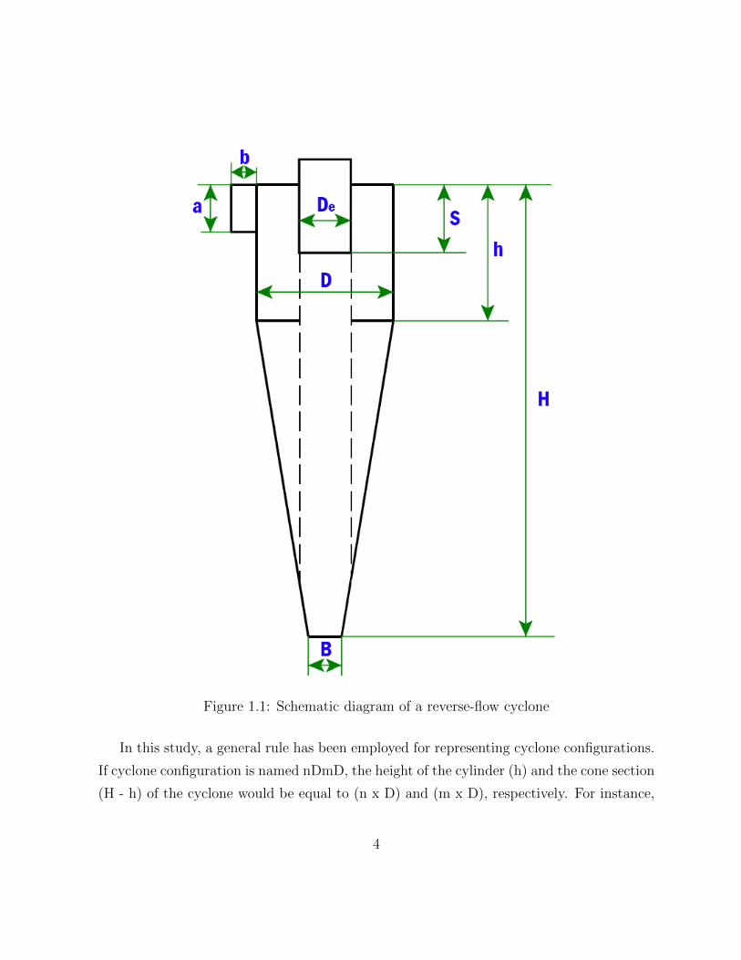
Figure 1.1: Schematic diagram of a reverse-flow cyclone

In this study, a general rule has been employed for representing cyclone configurations.

If cyclone configuration is named nDmD, the height of the cylinder (h) and the cone section

(H - h) of the cyclone would be equal to (n x D) and (m x D), respectively. For instance,

4

2D3D cyclone means a cyclone with cylinder height and cone height of two and three times

of cyclones diameter. The configurations of cyclones that are considered in this work are

1D3D [36], 2D2D [94], and 1D2D [96]. All the mentioned configurations are listed in Table

1.1. It should be noted that if the values of both H0 and h0 are set for any configuration

of the cyclone, the rest of the ratios will be known for that specific configuration.

Ratio Cyclone Cyclone Cyclone

1D3D 2D2D 1D2D

a0 = aD

0.5 0.5 0.5

b0 = bD

0.25 0.25 0.25

S0 = SD

0.125 0.125 0.625

De0 = DeD

0.5 0.5 0.625

H0 = HD

4 4 3

h0 = hD

1 2 1

B0 = BD

0.25 0.25 0.5

Table 1.1: Cyclone configuration ratio

1.3 Research objectives

The design of using a single cyclone connected to each particulate matter source device

is common in many industrial applications. In spite of the fact that each cyclone has

been designed with excellent performance to handle separation of particles, there are many

situations wherein a single cyclone is inadequate for the particle separation task. In such

5

situations, it is often feasible to use multiple units either in series or in parallel or both.

Therefore, the main objectives of this research are as follows:

1. To observe the feasibility to use multiple units of cyclone in actual NPK fertilizer

plant.

2. To develop a MINLP (Mixed Integer Nonlinear Programming) optimization model

in order to select the best arrangement of cyclones in parallel-series.

1.4 Outline of the thesis

This thesis is organized in five chapters as follows:

Chapter 2 presents the literature review on the key subjects covered in this work. The

studies relevant to the optimization of cyclone arrangement are reviewed. Several studies

have been conducted in experimental, theoretical, and computational research on cyclones

are also summarized in this chapter.

Chapter 3 present the nonlinear programming optimization of series and parallel cyclone

arrangement. The key idea in this work is to observe the feasibility to use multiple units

of cyclones in order to reduce the emissions in the actual Nitrogen, Phosphorus, and

Potassium (NPK) granulation plant. Furthermore, the best cyclone configurations and the

optimum arrangement whether in series or parallel are obtained by using GAMS software.

Chapter 4 presents a novel optimization of parallel-series cyclone arrangement. The key

novelties of the proposed method include the use of a mixed integer nonlinear programming

(MINLP) implemented in GAMS software to find the best cyclone arrangement with the

optimal number of cyclones and dimensions from several combinations of 1D3D and 2D2D

cyclone arranged in parallel-series. A case study with a total flow rate of 165 m3/s of a

stream to be processed in a paper mill is used to test the proposed method.

Chapter 5 summarizes the key research outcomes of the research avenues that can be

further explored in this area.

6

Chapter 2

Literature Review

2.1 Introduction

Cyclones are commonly used air pollution abatement devices for separating particulate

matter (PM) from air streams in industrial processes. Compared to other abatement sys-

tems, cyclones have low initial costs, maintenance requirements, and energy consumption.

There are basically two modeling approaches for evaluating the performance of a cyclone,

i.e, the equilibrium-orbit models and time-of-flight models. These models are based on a

force balance on a particle that is rotating in a cylindrical surface (CS) at radius Re = 12De.

Figure 2.1 (a) illustrates the concept of the equilibrium-orbit models. CS is formed by con-

tinuing the vortex finder wall to the bottom of the cyclone. Since there are two forces

in balance which are the centrifugal force and the inward drag caused by the gas flowing

through, large particles are centrifuged out from the cyclone wall and small particles are

dragged in and move out through the vortex tube. The particle size for which the two

forces balance (the size that orbits in equilibrium in CS) is taken as the dp or the cut-size

diameter. As such, it is the particle size that stands a 50-50 chance of being captured. This

particle size is very important in measuring the separation capability of the cyclone. Figure

2.1 (b) illustrates the other modeling approach, i.e., time-of-flight modeling. In this model,

7

the particle’s migration to the wall is considered, neglecting the inward gas velocity. The

total path length for a particle swirling close to the wall (assumed cylindrical) is: πDNi,

where Ni is the number of spiral turns the particle takes on its way toward the bottom of

the cyclone. The smallest particle size that can traverse the entire width of the inlet jet

before reaching the bottom of the cyclone as a critical particle size is considered as the

dp. It can be seen that the time-of-flight modeling concept is entirely different in nature

from the equilibrium-orbit concept. Although the time-of-flight models predict somewhat

larger cut sizes than the equilibrium-orbit models, the time-of-flight concept is found very

consistent with what is seen in CFD simulations. and it can become the most promising

for formulating models for the performance of cylindrical cyclones [55]. In addition, all the

equations used in this work will be derived from the time-of-flight model.

Figure 2.1: Sketches of the concept of: a. the equilibrium-orbit models, and b. the time-

of-flight models [55]

There are three main approaches on the study of cyclone performance in the literature:

8

• Mathematical models, which can be classified into: theoretical and semi-empirical

models, and statistical models

• Experimental measurements

• Computational fluid dynamics (CFD) simulations

Recently, a novel mathematical model of multiple cyclone arrangement has been de-

veloped. In addition, GAMS software also employed in the optimization [86] in order to

deliver the best results and reliable solutions.

2.2 Mathematical models

The theoretical or semi-empirical models of cyclones have been developed to acquire more

desirable understanding and prediction of cyclones’ performances to improve computation,

e.g., Alexander [3], First [28], Barth [6], Casal and Martinez-Benet [11], Stairmand [101],

Karagoz and Avci [59], Zhao [123], Avci and Karagoz [5], and Chen and Shi [12]. The ma-

jority of these models have been derived by using physical descriptions and mathematical

equations. These equations depend mainly on the characteristics of gas and particle motion

within the cyclone and energy dissipation mechanisms of cyclones. Over the years, interest

in particle collection and pressure drop of the cyclone theories has steadily increased. The

accuracy of the performance equations depends upon how well the assumptions made in

their development reflect the actual operating conditions within the cyclone. The most

widely used mathematical models of cyclone prediction performance are:

• Barth model [6]

• Stairmand model [101]

• Casal and Martinez-Benet model [11]

• Shepherd and Lapple model [94]

9

• The Muschelknautz method of modeling (MM) [55]

• Ramachandran model [82]

• Iozia and Leith model [57]

• Rietema model [85]

Some simplifying assumptions are common to all these models. They can be consid-

ered as offering a good compromise between accurate prediction and simplification of the

equations:

• The particles are spherical

• The radial velocity of the gas equals zero

• The radial force on the particle is given by Stokes law

2.2.1 Estimation of the cut-size diameter

• Barth model

Barth [6] proposed a simple model based on force balance (classified as one of the

equilibrium-orbit models [55]). This model considers the imaginary cylindrical sur-

face (CS) that is formed by continuing the vortex finder wall to the bottom of the

cyclone, see Figure 2.1. Here, all the gas velocity components are assumed constant

over CS for the computation of the equilibrium-orbit size. The Barth model for

theoretical cut-size diameter is given as below:

dp =

[9 µ De vrCSρp vθ2CS

] 12

(2.1)

where vrCS is the uniform radial gas velocity in the surface of CS given by:

vrCS =Q

π De HCS

(2.2)

10

HCS can be obtained by the following expression:

HCS =(R−Re) (H − h)

R− (B/2)+ (h− S) if B > De (2.3)

= (H − S) if B ≤ De (2.4)

• The Muschelknautz method of modeling (MM)

The cut-size diameter is analogous to the screen openings of an ordinary sieve or

screen [55]. In lightly loading cyclones, the cut-size exercises a controlling influence

on the cyclone’s separation performance that determines the horizontal position of the

cyclone grade-efficiency curve (fraction collected versus particle size). For low mass

loading, the cut-off diameter can be estimated in MM using the following equation:

dp =

[9 µ (0.9 Q)

π (ρp − ρ) vθ2CS (H − S)

] 12

(2.5)

• Iozia and Leith model

The Iozia and Leith model [57] is similar to the model of Barth [6] as it is also based

on the equilibrium-orbit theory. Iozia and Leith [57] gave the following expression

for the cut-size diameter:

dp =

[9 µ Q

π HCS ρp vθ2max

] 12

(2.6)

where:

HCS , the core height (height of the control surface of Barths model)

vθmax , the maximum tangential velocity, that occurs at the edge of the control surface CS

The value of the core diameter DCS and the tangential velocity at the core edge vθmax

are calculated from regression of experimental data using the following equations:

vθmax = 6.1 vi

(ab

D2

)0.61(De

D

)−0.74(H

D

)−0.33(2.7)

DCS = 0.52 D

(ab

D2

)−0.25(De

D

)1.53

(2.8)

11

• Rietema model

The Rietema model relates the cut-size diameter to pressure drop. Hence, the pres-

sure drop needs to be predicted to use the model. The following expression is used

to calculate the cut-size diameter:

dp =

[µ ρ Q

H (ρp − ρ) ∆P

] 12

(2.9)

A good pressure drop model for this purpose is that of Shepherd and Lapple [95].

The pressure drop (∆P ) based on the Shepherd and Lapple model is expressed in

term of the number inlet velocity heads of the gas (NH):

∆P =1

2ρv2iNH (2.10)

where:

NH =16ab

D2e

(2.11)

2.2.2 Estimation of the pressure drop

• Barth model

Barth subdivided the pressure drop into three contributions:

1. the inlet losses (Barth assumed that this loss could be effectively avoided by

good design)

2. the losses in the cyclone body

3. the losses in the vortex finder

12

The total pressure drop is the summation of the pressure drop in the cyclone body

∆Pbody and the pressure drop in the vortex finder ∆Px.

∆Pbody =1

2ρv2x

(De

D

) 1(vxvθCS− H−S

0.5Def)2 − (vθCSvx

)2

(2.12)

∆Px =1

2ρv2x

[(vθCSvx

)2

+Kx

(vθCSvx

) 43

](2.13)

where:

f , the friction factor

Kx , the vortex finder entrance factor

(Kx = 3.41 for rounded edge and Kx = 4.4 for sharp edge)

• The Muschelknautz method of modeling (MM)

According to the MM model, the pressure loss across a cyclone (∆P ) occurs, primar-

ily, as a result of friction with the walls (∆Pbody) and irreversible losses within the

vortex core (∆Px).

∆Pbody =fAR

0.9Q

ρ

2(vθCSvθw)1.5 (2.14)

∆Px =

[2 +

(vθCSvx

)2

+ 3

(vθCSvx

)4/3]

1

2ρv2x (2.15)

where:

AR , the total inside area of the cyclone contributing to frictional drag

vθw , the velocity in the vicinity of the wall

vx , the average axial velocity through the vortex finder

13

• Several expressions of empirical model have been developed to predict the cyclone

pressure drop. Most of the models express ∆P in terms of the number of inlet velocity

heads of the gas, NH .

∆P =1

2ρv2iNH (2.16)

The value of NH is usually a constant for geometrically similar cyclones of different

diameters. The most widely used equations are mentioned below:

– Stairmand model

Stairmand [101] estimated the pressure drop as entrance and exit losses com-

bined with the static pressure loss in the swirl.

NH = 1 + 2q2(

2(D − b)De

− 1

)+ 2

(4ab

πD2e

)2

(2.17)

– Sphered and Lapple model [95]

NH =16ab

D2e

(2.18)

– Casal and Martinez-Benet model [11]

NH = 3.33 + 11.3

(ab

D2e

)2

(2.19)

– Ramachandran model

The Ramachandran et al. [82] model was developed through a statistical anal-

ysis of pressure drop data for ninety-eight cyclone designs.

NH = 20

[ab

D2e

] [ SD

HDhDBD

] 13

(2.20)

14

2.3 Experimental methods

There are numerous experimental measurements performed on the cyclone separators.

Some of the studies measured the pressure drop and collection efficiency. For example,

Dirgo and Leith [17] measured the collection efficiency and pressure drop for the Stair-

mand high efficiency cyclone at different flow rates. Hoffmann et al. [54] investigated the

effect of cyclone length on the separation efficiency and the pressure drop experimentally

and theoretically by varying the length of the cylindrical segment of a cylinder-oncone

cyclone. They found for cyclone lengths from 2.65 to 6.15 cyclone diameters, a marked

improvement in cyclone performance is achieved with increasing length up to 5.5 cyclone

diameters; beyond this length the separation efficiency was dramatically reduced. Other

experimental results on cyclones can also found in [119, 100, 76, 60, 52, 53, 16]. The major-

ity of these models have focused on the development of single cyclones. Other researchers

established experiments to observe the performance of multi cyclone arrangements. Gillum

et al. [40] investigated the arrangement of an existing 2D2D cyclone connected to 2D2D

cyclone for the first test and to a 1D3D cyclone for the second test. Gillum and Hughs

[39] held an experiment with the variation of the inlet velocity ranged from 11.8 to 18.3

m/s through two cyclones in series, 2D2D primary and 2D2D or 1D3D secondary. Colum-

bus [15] also studied a 2D2D primary cyclone in series with a 1D3D secondary cyclone

in capturing particulate matters (PM) emitted from a seed cotton separator. Whitelock

and Buser [118] evaluated the effectiveness of up to four 1D3D cyclones in series on heavy

loading of particulate air streams (236 g/m3). These studies showed that the series ar-

rangement had a significant improvement in cyclone overall efficiency compared to a single

cyclone. However, having the two cyclones in series appeared to be the best choice because

of the use of three or four cyclones in series only slightly increased the overall efficiency

along with a significant increase in the pressure drop across all cyclones [118].

15

2.4 Computational fluid dynamics (CFD) simulations

The CFD technique became a widely used approach for the flow simulation and perfor-

mance estimation of cyclone separators. The CFD modeling approach is able to predict

the features of the cyclone flow field in great details, which provide a better understanding

of the fluid dynamics in cyclone separators [43]. The pressure drop predicted by CFD was

also found in an excellent agreement with measured data. Moreover, Gimbun et al. [41]

successfully applied CFD to predict and to evaluate the effects of temperature and inlet

velocity on the pressure drop of gas cyclones. This makes the CFD methods represent a

reliable and cost-effective route for geometry optimization in comparison with the experi-

mental approach. However, CFD is still more expensive in comparison with the simplified

mathematical modeling approach. The main reasons behind the cost of the CFD approach

with respect to the mathematical methods are:

• The license cost of the grid generator, solver and post processor

• The running cost especially for unsteady state simulations which need also parallel

processing

• The CFD process requires expert intervention by an expert researcher at every stage

(mesh generation, solver settings and post processing)

• CFD results always need validation with experimental results, and perform the same

simulation on different grids to be sure that the obtained results are grid independent.

2.5 Mathematical programming models

Mathematical programming provides a general modeling framework for optimization that

finds many interesting applications in chemical engineering. For example, linear program-

ming (LP) has been extensively used for refinery scheduling and batch production planning

16

problems (e.g., Symonds [105], Mauderli and Rippin [73]). Mixed integer linear program-

ming (MILP) has been used for the synthesis of process systems with simplified mod-

els (e.g., Grossmann and Santibanez [50], Papoulias and Grossmann [74]), and for batch

scheduling (e.g., Rich and Prokopakis [84], Ku and Karimi [66], Kondili et al. [64], Shah

et al. [93], Pinto and Grossmann [79]). Nonlinear programming (NLP) has been used for

separation process design and optimization (e.g., Sargent and Gaminibandara [91], Ku-

mar and Lucia [67]). Mixed-integer nonlinear programming (MINLP) has been used for

process synthesis (e.g., Grossmann [44, 48, 45, 46], Duran and Grossmann [21], Kocis and

Grossmann [62, 63], Floudas and Paules [32], Kravanja and Grossmann [65], Grossmann

and Kravanja [49]), distillation design (e.g., Viswanathan and Grossmann [109, 110], Ciric

and Gu [13]), process scheduling (e.g., Sahinidis and Grossmann [90], Tsirukis et al. [106],

Pinto and Grossmann [78]), process control strategy (e.g., [92]), and pump configurations

(e.g., Pettersson and Westerlund [77], Westerlund et al. [117] ). The application of these

mathematical programming tools has provided useful results. Moreover, NLP and MINLP

techniques are applied in the present work for multiple cyclone arrangement problems.

2.5.1 Nonlinear Programming (NLP) models

The nonlinear programming problem can be defined as follows:

Min f(x)

s.t. h(x) = 0

g(x) ≤ 0

Sufficient conditions that guarantee global optimality are that f(x) convex, h(x) lin-

ear, and g(x) convex. These nonlinear programming models and techniques are frequently

used in the optimization of process systems in chemical engineering. However, these NLP

models often include non-convex functions (e.g., f(x) and g(x) concave, h(x) nonlinear)

that give rise to multiple suboptimal solutions and non-optimal stationary points. Conse-

quently, a solution obtained for a non-convex model with a standard optimization algorithm

17

(e.g., generalized reduced gradient, successive quadratic programming) which is commonly

rigorous for convex problems, is strongly dependent on the starting point. Moreover, lin-

earizations of non-convex constraints of feasible problems can define infeasible regions or

produce indefinite Hessian matrices that often cause the failure of standard local optimiza-

tion techniques [70].

The problem of determining a global optimum solution for non-convex NLP problems is

generally very difficult. No algorithm can solve a general and smooth global optimization

problem with certainty in a finite number of steps, unless some kind of tolerance for the

precision of the global minimum is pre-specified [18]. Depending on whether global opti-

mization techniques incorporate stochastic elements or not, they are classified as stochastic

or deterministic [19]. Stochastic techniques are applicable to optimization problems that

do not exhibit special structures, but can not guarantee convergence to a global optimum

in finite time. Deterministic global optimization techniques on the other hand are designed

to converge to a global optimum solution with certainty or to prove that such a point does

not exists. To provide this kind of guarantee, deterministic techniques make a number of

specific assumptions and restrict their applicability to specific classes of problems. Excel-

lent surveys on deterministic techniques and more references to the literature can be found

in Horst [56].

The issue of non-convex optimization and the concern for finding global optimal solu-

tions have been present in the chemical engineering literature since the pioneering work

by Stephanopoulos and Westerberg [102]. A non-deterministic approach for the solution

of non-convex models in chemical engineering includes the works by Kocis and Grossmann

[63], Floudas et al. [30], Floudas and Ciric [31], Viswanathan and Grossmann [108], Floudas

and Aggarwal [34]. Deterministic algorithms for the global optimization of certain classes of

NLP models in chemical engineering can be found in the following citations: the GOP algo-

rithm by Floudas and Visweswaran [33, 35], the branch and bound algorithm for factorable

programs by Swaney [104] and Epperly and Swaney [24], the global optimization algorithm

for rationally constrained rational programming problems by Manousiouthakis and Sourlas

[71], the interval global optimization algorithm by Vaidyanathan and El-Halwagi [107], the

18

branch and bound algorithm for programs with linear fractional and bilinear terms by Que-

sada and Grossmann [81], the branch and reduce algorithm by Ryoo and Sahinidis [88, 89],

the αBB algorithm by Androulakis et al. [4], and the reformulation spatial branch and

bound algorithm for general process models by Smith and Pantelides [98].

2.5.2 Mixed Integer Nonlinear Programming (MINLP) models

A mixed integer program (MIP) is an optimization problem that involves continuous as

well as integer variables. The most frequent case of MIP is the one in which the integer

variables are restricted to be of the 0 - 1 type (binary variables):

Min f(x, y)

s.t. h(x, y) = 0

g(x, y) ≤ 0

x ε Rn , y ε {0, 1}m

A MIP is said to be linear (MLP) if the objective function and the constraints that

define the feasible set are linear, otherwise the MIP is said to be nonlinear (MINLP). For

the case of an MILP the LP relaxation is convex. Thus, global optimality can be guaranteed

with a branch and bound algorithm since rigorous lower bounds are predicted. When the

values of all the integer variables in a MINLP are fixed, a NLP problem in the continuous

subspace is obtained. Both, MILPs and MINLPs are non-convex programs since they have

disconnected feasible regions due to their discrete nature. Hence, non-convexities may also

arise in the feasible subspace for the continuous variables (e.g., f(x,y), g(x,y) non-convex

for fixed y, h(x,y) nonlinear for fixed y). A MINLP model is said to be non-convex if the

relaxation of the integrality condition yields a non-convex NLP problem.

There has been recently an increased interest in the development of mixed integer

nonlinear programming (MINLP) in the area of engineering design, planning, scheduling

and marketing. Several techniques for the solution of MINLP models are Generalized

19

Benders Decomposition, GBD (Geoffrion [37]), the branch and bound method (Gupta and

Ravindran [51]), Outer Approximation / Equality-Relaxation Method OA/ER (Duran and

Grossmann [22], Kocis and Grossmann [62], Fletcher and Leyffer [29]), the LP/NLP based

branch and bound technique (Quesada and Grossmann [80]), and the extended cutting

plane method (Westerlund and Pettersson [116]). Detailed descriptions of these techniques

and extensive references on the subject can be found in Grossmann and Kravanja [49].

It is well known that, when applied to non-convex MINLP models, these techniques

might get trapped at suboptimal solutions, or even worse, they may fail to obtain a feasible

point. Viswanathan and Grossmann [108] proposed a heuristic strategy that aims at re-

ducing the effect of non-convexities. The proposed model combined Outer Approximation

/ Equality-Relaxation (OA/ER) method with an Augmented Penalty (AP) function. The

proposed algorithm has as main features that it starts with the solution of the NLP relax-

ation problem, and that it features an MILP master problem with an augmented penalty

function that allows violations of linearizations of the nonlinear functions. This scheme

provides a direct way of handling non-convexities which are often present in engineering

design problems. The main steps in the proposed AP/OA/ER algorithm are as follows:

• Step 1:

Solve the relaxed NLP problem in (1) to determine a KKT point (x0, y0). If y0 is an

integer, the solution is found, stop. Otherwise, set K = 0, zOLD = +∞ , and go to

Step 2.

• Step 2:

Set up the MILP master problem and solve to find the integer vector yK+1.

• Step 3:

Solve the NLP subproblem [P (yK+1)] to determine the KKT point (xK+1, yK+1) with

objective value zK+1. If the NLP is infeasible set FLAG = 0. If the NLP is feasible

set zNEW = zK+1, FLAG = 1.

• Step 4:

20

(a) If FLAG = 1, determine if zNEW > zOLD; if satisfied, stop. The optimal solution

is zOLD. Otherwise, set zOLD = zNEW , set K = K + 1 and return to Step 2 by adding

the corresponding linearization and integer cut.

(b) If FLAG = 0, set K = K + 1 and return to Step 2 by adding the integer cut.

It should be noted that the above algorithm will terminate in one iteration if an integer

solution is found in Step 1, or else it will terminate after three or more iterations when the

termination condition in Step 4 (a) is satisfied. Note that in the latter case, N iterations

imply the solution of N NLP subproblems, and N-1 MILP subproblems. Also, it should

be noted that since at each iteration K ≥ 1, an integer cut is added to the MILP master

problem in Step 2 (even for the case of infeasible NLP subproblems), the algorithm cannot

cycle and return to an integer point that has been previously examined. Finally, if convexity

of the MINLP can be established a priori, the termination criterion in Step 4 can be replaced

by the use of the lower bound predicted by the MILP master problem as in the OA/ER

algorithm.

It is also important to note that although the proposed algorithm has provisions for

trying to overcome the effect of non-convexities, it can fail to find the global optimum

mainly for the two following reasons. Firstly, if the NLP relaxation has multiple local so-

lutions with integer points, then clearly the algorithm can converge to a suboptimal point.

Secondly, if the NLP subproblem for fixed binary values has different local optima, the

algorithm may be trapped into a local solution. Despite these limitations, the numerical

performance, which has been tested on a variety of applications has shown that the compu-

tational requirements of this method are quite reasonable while providing a high degree of

reliability for finding global optimum solutions. The proposed algorithm by Viswanathan

and Grossmann [108] has been implemented in DICOPT [25] as part of the solver that

runs under GAMS software [86] which is used to solve the multiple cyclone arrangement

problems in the present work.

21

Chapter 3

Nonlinear programming optimization

of series and parallel cyclone

arrangement of NPK fertilizer plants

This chapter presents a nonlinear programming optimization to address the optimal num-

ber and configuration of series and parallel cyclone arrangement in the NPK fertilizer

plant. The organization of this chapter is as follows: an overview of process of actual NPK

granulation fertilizer plant is given in Section 3.1. Next, Section 3.2 presents the objective

of the study. The equations employed in the modeling is presented in Section 3.3. The

mathematical models of parallel cyclone arrangement and series cyclone arrangement are

presented in Section 3.4 and Section 3.5, respectively. The results of the optimization of

three types of cyclone (i.e., 1D3D, 2D2D, and 1D2D) using parallel arrangement and series

arrangement are presented in Section 3.7. Section 3.8 summarizes the methodology and

work presented in this chapter. The content of this chapter has been published in Powder

Technology [2] (see Appendix A).

22

3.1 Overview of process of actual NPK granulation

fertilizer plant

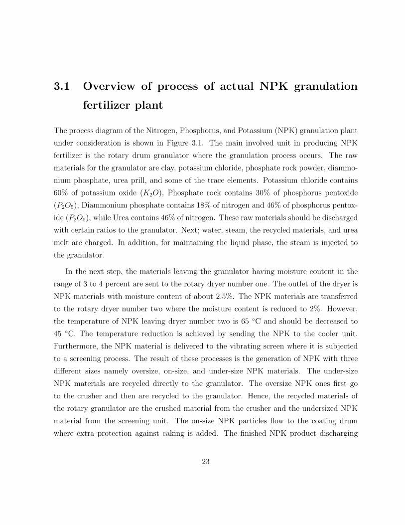
The process diagram of the Nitrogen, Phosphorus, and Potassium (NPK) granulation plant

under consideration is shown in Figure 3.1. The main involved unit in producing NPK

fertilizer is the rotary drum granulator where the granulation process occurs. The raw

materials for the granulator are clay, potassium chloride, phosphate rock powder, diammo-

nium phosphate, urea prill, and some of the trace elements. Potassium chloride contains

60% of potassium oxide (K2O), Phosphate rock contains 30% of phosphorus pentoxide

(P2O5), Diammonium phosphate contains 18% of nitrogen and 46% of phosphorus pentox-

ide (P2O5), while Urea contains 46% of nitrogen. These raw materials should be discharged

with certain ratios to the granulator. Next; water, steam, the recycled materials, and urea

melt are charged. In addition, for maintaining the liquid phase, the steam is injected to

the granulator.

In the next step, the materials leaving the granulator having moisture content in the

range of 3 to 4 percent are sent to the rotary dryer number one. The outlet of the dryer is

NPK materials with moisture content of about 2.5%. The NPK materials are transferred

to the rotary dryer number two where the moisture content is reduced to 2%. However,

the temperature of NPK leaving dryer number two is 65 ◦C and should be decreased to

45 ◦C. The temperature reduction is achieved by sending the NPK to the cooler unit.

Furthermore, the NPK material is delivered to the vibrating screen where it is subjected

to a screening process. The result of these processes is the generation of NPK with three

different sizes namely oversize, on-size, and under-size NPK materials. The under-size

NPK materials are recycled directly to the granulator. The oversize NPK ones first go

to the crusher and then are recycled to the granulator. Hence, the recycled materials of

the rotary granulator are the crushed material from the crusher and the undersized NPK

material from the screening unit. The on-size NPK particles flow to the coating drum

where extra protection against caking is added. The finished NPK product discharging

23

from the coating machine is lifted by the product elevator into the product hopper, where

it is measured and packaged by an automatic packing machine before being sent into the

warehouse.

Through the above-mentioned processes, there are several sources of pollution-emitting

particulates. These particulates are released from the two types of dryers, the cooler, and

the vibrating screen. To control the emissions of particulate matter, the plant operates

with four cyclones. Each cyclone will be connected to each particulate matter source device

(i.e., dryer 1, dryer 2, cooler, and vibrating screen).

24

Figure 3.1: Process diagram of NPK granulation fertilizer

25

3.2 Objective of the study

Cyclone is used as a first stage to control the emissions of particulate matter in NPK

granulation fertilizer plant. These particulate matters are actually the part of raw materials

that can be used to produce again the NPK fertilizer by sending it to the granulator. In

order to maintain a low losses in the plant, the performance of those cyclones as a dedusting

system must be satisfied. Despite all the cyclones have been designed with high efficiency,

high production targets may lead to decrease efficiency of the cyclone.

While the NPK fertilizer plant must be operated at its maximum capacity, an im-

provement of cyclone operation to maintain the low emissions should be sought. There

are several options available to reach an optimum operating condition of cyclone. Each

of these options has associated with a certain cost and a certain reduction capability. In

this work, it is desired to observe a feasibility to use multiple units of cyclone in order

to reduce the emissions. Furthermore, the best cyclone configurations and the optimum

arrangement whether in series (Figure 3.3) or parallel (Figure 3.2) will be resulted from

simulation using NLP model. The objective function is to minimize the total cost, includ-

ing the operating cost and the capital cost. It is noted that the objective of the present

study is not to compare the two types of arrangements but instead to determine the most

suitable arrangement for a given fertilizer plant under study and optimize its configuration

and dimensions.

3.3 The equations employed in the modeling

3.3.1 Equation for the cut-size diameter

In a gas-solid cyclone, the solid particles are mostly moving at their terminal velocity

with respect to the gas. Therefore, the terminal velocity of a given solid particle decide

whether the particle would be captured by the cyclone or not (i.e., escape to the atmosphere

26

or not). The terminal velocity is exactly analogous to that of a particle settling in the

earth’s gravitational field (g) under steady-state conditions. However, for a cyclone, the

gravitational force is replaced by the radially directed centrifugal force [55] as shown in

Eq.(3.1).

FG = mp

(v2θr

)(3.1)

where:

FG , the downward force of gravity acting on the particles (N)

mp , the mass of the particle (kg)

vθ , the tangential velocity of particle (m/s)

r , the radius of particle (m)

A viscous drag force is experienced when any object rises through fluid. If viscous

drag force happens inside the cyclone with assumption of no slip between the fluid and the

particle surface (i.e., at the surface of the particles, the velocity would be the same as the

fluid one), then the Stokess drag law Eq.(3.2) can be applied for mathematical modeling

[9].

Fd = 3πµdpvt (3.2)

where:

Fd , the drag force of the fluid on a sphere (N)

dp , the particle diameter (m)

µ , the dynamic viscosity (Ns/m2)

vt , the terminal velocity of particle (m/s)

27

When the solid particle falls, the particle velocity increases until it reaches a velocity

known as the terminal velocity. The centrifugal force quickly accelerates the particle to its

terminal velocity in the radial direction. At this constant velocity, the frictional drag due

to viscous forces is balanced by the gravitational force. By combining Eqs.(3.1) and (3.2),

Eq.(3.3) is produced as the following:

vt =2 mp v

2i

3 π µ dp D(3.3)

where

vi = vθ , the gas inlet velocity (m)

r = D/2 (m)

Clift et al. [14] defined the mass of the particle (mp) moving with steady terminal

velocity in a gravitational field as follows in Eq.(3.4).

mp =

(πd3p6

)(ρp − ρ) (3.4)

where:

ρp , the particle density (kg/m3)

ρ , the gas density (kg/m3)

Substituting Eq.(3.4) into Eq.(3.3) yields Eq.(3.5).

vt =d2p (ρp − ρ) v2i

9 µ D(3.5)

Moreover, Rosin et al. [87] proposed the time-flight model that compared the time

required for a particle injected through the inlet of the cyclone at some radial positions

to reach the cyclone wall and travel the entire width of the inlet jet before reaching the

bottom of the cyclone. Assuming the inlet velocity of the particles prevail at the cyclone

28

wall, the required time for the particle to reach the bottom of the cyclone (∆t in seconds

can be described as shown in Eq.(3.6).

∆t = cylinderical path length / velocity =π D Ni

vi(3.6)

Besides Ni is the number of spiral turns of particle inside the cyclone that can be

calculated using the Lapple’s expression from Eq.(3.7).

Ni =1

a

[h+

(H − h)

2

](3.7)

The maximum radial distance traveled by any particle is the width of the inlet duct.

The terminal velocity vt that allows a particle initially at distance b away from the wall to

be collected in time ∆t is represented in Eq.(3.8).

vt =b

∆t(3.8)

Substituting Eqs.(3.6) to (3.8) yields Eq.(3.9).

vt =b vi

π D Ni

(3.9)

The smallest particle diameter that just traverses the entire width of the inlet duct to

the wall and is collected can be obtained by setting the two expressions for vt equal to

each other and rearranging Eq.(3.5) with Eq.(3.9). Eq.(3.10) is obtained for the cut-size

diameter.

dp =

[9 µ b

π Ni (ρp − ρ) vi

] 12

(3.10)

The so-called cut-size diameter (dp) is very essential as it is used in the model for the

calculation of the particle collection efficiency [6]. It is assumed that the cyclone has a sharp

cut at dp (i.e., all particles’ size below dp is lost to the atmosphere and all particles’ size

above it is captured by the cyclone). By comparing the real efficiency found by experiments

with the calculated one from the cut-size (predicted by the model), it is discovered that

the results are highly accurate. This is true even when the cut-size diameter of the cyclone

is far from sharp particles [55].

29

3.3.2 Equation for the pressure drop

The pressure drop of the cyclone in this work is expressed as the number of inlet velocity

heads of the gas, NH . The model from Casal and Martinez-Benet [11] is used to calculate

the cyclone pressure drop as shown in Eq.(3.11).

∆P =1

2ρ v2i NH (3.11)

where:

NH = 11.3

(a b

D2e

)2

+ 3.33 (3.12)

3.3.3 Equation for the cost per unit of cyclone

The total cost per unit of cyclone, ctot ($/s) is the summation of the operating cost (copr)

and the capital cost (ccap).

ctot = copr + ccap (3.13)

The operating cost (copr) and the capital cost (ccap) are calculated by Martinez-Benet

and Casal [72] equations as shown in Eqs.(3.14) and (3.15) respectively.

copr = Q ∆P ce (3.14)

where:

ce , the cost of utilities (= $ 1.5 x 10−8/J [97])

ccap =F e

Y twN Dj (3.15)

30

where:

F , the investment factor (= 4.4 [99] )

Y , the number of years over which depreciation occurs (= 5)

tw , the time worked per year (= 2.16 x 107s/year)

e , constant (= $ 4924.61/m) that is obtained from Eq.(3.16)

j , constant (= 1.2) that its value depends on the equipment type [99]

e =CB fM fP fT

DBj (3.16)

where the following values are obtained from Smith [99] :

CB , the known base cost for cyclone with diameter DB (= $ 1640)

DB , the cyclone base diameter (= 0.4 m)

fM , the correction factor for materials of construction (= 1)

fP , the correction factor for design pressure (= 1)

fT , the correction factor for design temperature (= 1)

3.4 Mathematical models of parallel cyclone arrange-

ment

For parallel cyclone arrangement, the diameter of the cyclone (Dp, m), the inlet velocity

(vip , m/s), and the pressure drop (∆Pp, N/m2) are variables that will be optimized. The

flow rate of each cyclone in parallel arrangement (Qp, m3/s), the inlet velocity (vip , m/s),

and the pressure drop (∆Pp, N/m2) can be calculated from Eqs.(3.17 - 3.19).

31

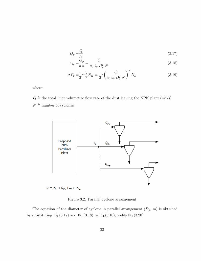
Qp =Q

N(3.17)

vip =Qp

a b=

Q

a0 b0 D2p N

(3.18)

∆Pp =1

2ρv2ipNH =

1

2ρ

(Q

a0 b0 D2p N

)2

NH (3.19)

where:

Q , the total inlet volumetric flow rate of the dust leaving the NPK plant (m3/s)

N , number of cyclones

Figure 3.2: Parallel cyclone arrangement

The equation of the diameter of cyclone in parallel arrangement (Dp, m) is obtained

by substituting Eq.(3.17) and Eq.(3.18) to Eq.(3.10), yields Eq.(3.20)

32

Dp =

[d2p (ρp − ρ) π Ni

9 b20 a0 µ

Q

N

]1/3(3.20)

The objective function is total cost of parallel cyclone arrangement (ctotp) minimization

and calculated from the following expression:

MIN ctotp = Q ∆Pp ce +F e

Y twN Dj

p (3.21)

3.5 Mathematical models of series cyclone arrange-

ment

Figure 3.3: Series cyclone arrangement

In this arrangement, the cyclones are connected in series as shown in Figure 3.3. This

arrangement is set to have up to 3 cyclones with similar diameters. The diameter of the

33

first cyclone is calculated by using Eq.(3.20) with N = 1.

Ds1 =

[d2p1 (ρp − ρ) π Ni Q

9 b20 a0 µ

]1/3(3.22)

where Ds1 is the diameter of primary cyclone.

Meanwhile, as seen in the figure, the overflow mass of the particles (mp) from the first

cyclone that is charged to the next cyclone will be affected by the efficiency of the previous

cyclone as indicated in Eqs.(3.23) and (3.24).

mp1 = mp

mp2 = (1− η1) mp1 = (1− η1) mp (3.23)

mp3 = (1− η2) mp2 = (1− η1)(1− η2) mp (3.24)

Based on the definition of mass particle by Clift et al. [14], Eq.(3.4) can be substituted

into Eqs.(3.23) and (3.24), yields Eqs.(3.25) and (3.26).

mp2 = (1− η1)(πd3p2

6

)(ρp − ρ) (3.25)

mp3 = (1− η1) (1− η2)(πd3p3

6

)(ρp − ρ) (3.26)

Moreover, the equation for calculating the diameter of the second (Ds2 , m) and third

(Ds3 , m) cyclone is obtained by rearranging Eqs.(3.3) and (3.9).

Ds2 =

[2 mp2 Ni Q

3 dp2 b20 a0 µ

]1/3(3.27)

Ds3 =

[2 mp3 Ni Q

3 dp3 b20 a0 µ

]1/3(3.28)

Substituting Eq.(3.25) into Eq.(3.27) and Eq.(3.26) into Eq.(3.28) yields Eq.(3.29) and

Eq.(3.30), respectively.

Ds2 =

[d2p2 (1− η1) (ρp − ρ) π Ni Q

9 b20 a0 µ

]1/3(3.29)

Ds3 =

[d2p3 (1− η1)(1− η2) (ρp − ρ) π Ni Q

9 b20 a0 µ

]1/3(3.30)

34

While the flow rate for each cyclone in series arrangement would be the same, the inlet

velocity (vis , m/s) and the pressure drop (∆Ps, N/m2) are calculated from Eqs.(3.31 -

3.32).

vis =Q

a b=

Q

a0 b0 D2s

(3.31)

∆Ps =1

2ρv2isNH =

1

2ρ

(Q

a0 b0 D2s

)2

NH (3.32)

For the series cyclone arrangement, it has two objective function problem. In this

problem, the overall efficiency (ηov) of the cyclone is maximized while the total cost of two

series cyclones and three series cyclones are minimized. The total cost is minimized by

following expression:

MIN ctots = Q

NS∑s=1

∆Ps ce +

[F e

Y tw

NS∑s=1

Djs

](3.33)

NS , number of stage of the arrangement

The overall efficiency of the series cyclone arrangement has relationship with the effi-

ciency of each cyclone as illustrated in Figure 3.4 and can be calculated as given in Eqs.(3.34

- 3.35).

35

Figure 3.4: Illustration of the overall efficiency of the series cyclone arrangement

For 2 cyclones in series: ηov =1− [ (1− η1)(1− η2) ] (3.34)

For 3 cyclones in series: ηov =1− [ (1− η1)(1− η2)(1− η3) ] (3.35)

36

3.6 Constraints

The constraints of optimization model are related mainly to the pressure drop and the inlet

velocity. According to Buonicore et al. [10] the pressure drop of the cyclone arrangement

will have the upper bound (∆PL) and the lower bound (∆PU) and is normally accepted

to be in the range as shown in Eq.(3.36).

500 ≤ ∆P ≤ 2500 N/m2 (3.36)

In terms of the inlet velocity, Gimbun et al. [41] reported that for identical size and

configuration of cyclone, the higher the gas inlet velocity is, the higher the efficiency would

be. Nevertheless, a very high inlet velocity would decrease the collection efficiency because

of increased turbulence and probability of saltation/re-entrainment of particles. Shepherd

and Lapple [94] proposed the range of practicable cyclone inlet velocity which is shown in

Eq.(3.37).

15 ≤ vi ≤ 30 m/s (3.37)

Moreover, according to Koch and Licht [61], to avoid re-entrainment of particles inside

the cyclone, the inlet velocity should be less than 1.35 times the saltation velocity (vs).

vs = 4.91

(4gµ(ρp − ρ)

3ρ2

)1/3b0.40

(1− b0)1/3D0.067 v

2/3i (3.38)

The maximum inlet velocity of the cyclone has to be controlled in order not to exceed

the maximum allowable pressure drop. The maximum value of inlet velocity must comply

with its equation that is defined by Eq.(3.39).

vimax =

√2 ∆Pmaxρ NH

=

√2 (2500)

ρ NH

(3.39)

In summary, the lower (vLi ) and the upper (vUi ) constraints of the inlet velocity of the

cyclone become those expressed in Eq.(3.40).

15 m/s ≤ vi ≤ min (30 m/s , 1.35vs , vimax) (3.40)

37

According to Smith [99], the size range of the diameter of the cyclone of which becomes

the lower (DL) and upper limit (DU) of the diameter of the cyclone in the optimization

model can be shown in Eq.(3.41).

0.4 ≤ D ≤ 3 m (3.41)

In addition for the series cyclone arrangement, it is desired to maximize the overall

efficiency with the following constraints:

0.99 ≤ ηov ≤ 1 (3.42)

where the efficiency of each cyclone based on the experimental result of multiple series

cylones by Whitelock and Buser [118] has ηL and ηU as given below:

For cyclone No.1: 0.9 ≤ η1 ≤ 0.99 (3.43)

For cyclone No.2: 0.55 ≤ η2 ≤ 0.99 (3.44)

For cyclone No.3: 0.2 ≤ η3 ≤ 0.99 (3.45)

3.7 Results and discussion

All mathematical models have been implemented and solved in GAMS (General Algebraic

Modeling System, [86]) in a CPU Intel Core i5-4200U, 1.60 GHz. CONOPT 3 solver [20]

was used to solve the NLP problem.

The input feed as the parameters for both cyclone arrangements (parallel and series) to

be processed is described in Table 3.1. The flow rate of input feed to the cyclones in both

arrangements is roughly the sum of all particulates’ flow rate that is generated from the

two dryers, the cooler, and the screen of the proposed NPK plant. These data are used to

calculate the optimal number of cyclones (N) of parallel arrangement while minimizing the

total cost. In addition, to compute the value of optimal number of cyclones, the models

38

Parameter Value

Q 13.97 (m3/s)

ρp 1042.0 (kg/m3)

ρ 1.33 (kg/m3)

µ 19.34 x 10−6(N.s/m2)

dp 21.63 x 10−6(m)

Table 3.1: Specification of input feed to the cyclone

calculate the optimal value of the pressure drop, the inlet velocity, and the diameter of the

cyclone. The diameter of the cyclone has an important role in the resultant value of the

pressure drop and the inlet velocity in this optimization. Therefore, after determination

of the optimal number of cyclones with minimum cost, the optimal value of the diameter

of the cyclone is obtained. Moreover, the value of the optimal diameter of the cyclone is

used to calculate the optimal pressure drop and inlet velocity. Another value that affects

the result of the optimization model is the value of efficiency of the cyclone, however this

only applies for the series cyclone arrangement (Figure 3.3).

The obtained optimal number of cyclones lies within the constraints of the pressure drop

of the cyclone, the inlet velocity, and the diameter of the cyclone. An interesting result

arises in the optimization of which the optimal number of cyclones lies at the upper bound of

the diameter. The selection of the upper bound of the diameter as the optimal value of the

decision variable can be explained physically wherein by increasing the cyclone diameter,

the residence time also increases. The increase in the available time for collection of

particles results in an increase in the total collection efficiency. So, the optimal performance

of the cyclone can be reached.

After the first trial, the constraint of the diameter as shown in Eq.(3.41) does not lead

to draw a specific inference when it is used to find the optimal number of cyclones. This

is probably due to a big gap between the lower bound and upper bound of the diameter.

In order to obtain a specific result of the optimal number of cyclones, the constraint of

39

the diameter is modified. The constraints of the diameter of the cyclone are divided into

five parameters (i.e., each parameter has a lower limit of 1.2 m and an upper limit varying

between 1.8 m, 2.0 m, 2.5 m, 2.7 m, and 3.0 m). Moreover, these new constraints would

be used to calculate the optimal number of the cyclone for each arrangement (i.e., parallel

and series).

The resultant value of the optimization of the parallel 1D3D cyclone arrangement can

be seen in Table 3.2. The optimal values of number of cyclones, the cyclone diameter,

the cyclone pressure drop, and the inlet velocity of the cyclone of 1D3D cyclone were

obtained by using the upper bound of diameter up to 2.5 m. Meanwhile, for the 2D2D

cyclone (Table 3.3) and 1D2D cyclone (Table 3.4) the values of the optimal parameters

are obtained using the upper bound of diameter up to 3.0 m and 2.7 m, respectively. The

effects of the constraint of cyclone diameter on the results of optimal number of each type

of cyclones connected in parallel are presented in Figure 3.5. The 1D3D cyclones connected

in parallel have the smallest diameter for the same value of optimal number of cyclones (N

= 3) compared with the other two. Using an upper bound diameter up to 3.0 m, the 2D2D

cyclone with parallel arrangement model resulted in one cyclone as the optimal number of

cyclones.

Furthermore, the simulation results obtained from the present mathematical program-

ming models were also compared with the outputs of some other models, such as Yetilmez-

soy’s optimum body diameter (OBD) model [121, 122] and KalenZenz’s model [58]. De-

tailed mathematical definitions of these models and relevant calculation procedures can be

found in the studies of Yetilmezsoy [121, 122]. Based on the present input data (Q = 13.97

m3/s, ρp = 1042kg/m3, design temperature = 45 oC, a0 = a/D = 0.50, and b0 = b/D =

0.25), all models were evaluated for each type of cyclones (i.e., 1D3D, 2D2D, and 1D2D)

connected in parallel, and the numerical outputs (i.e., cyclone diameter and pressure drop)

were compared with the optimization results given in Tables 3.2 - 3.4. Table 3.5 lists

comparisons of cyclone diameters and pressure drops predicted by the different models for

1D3D, 2D2D, and 1D2D cyclones at their own gas outlet diameter of the cyclone ratio

(De0 = De/D), i.e., 0.50, 0.50 and 0.625, respectively.

40

Table 3.2: Optimization results from GAMS code for 1D3D cyclones in parallel

41


42


43

Figure 3.5: Optimal solution of parallel cyclone arrangement

44

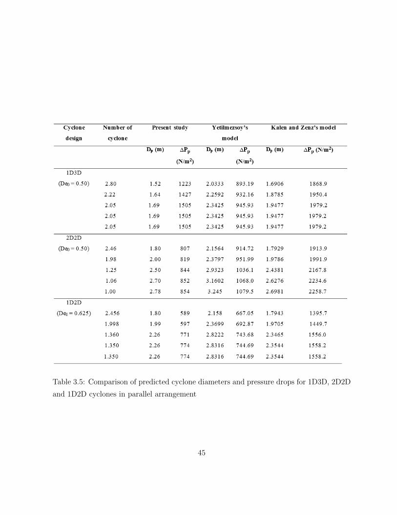
Table 3.5: Comparison of predicted cyclone diameters and pressure drops for 1D3D, 2D2D

and 1D2D cyclones in parallel arrangement

45

The comparisons illustrated that the present study gave pressure drop predictions that

were closest to the outputs obtained from the empirical methodology proposed by Yetilmez-

soy [121, 122]. On the other hand, the numerical results in Table 3.5 confirmed that cyclone

diameters obtained by the present study (GAMS code) were much closer to the theoretical

outputs for 2D2D cyclone design than those calculated for 1D3D and 1D2D cyclones in

parallel arrangement.

The cyclone configuration of series arrangement is influenced by the optimization of the

efficiency of each cyclone. For example, the optimal configuration of two 1D3D cyclones in

series will have 2.7 m of cyclone diameter with 97.8% of cyclone No.1 efficiency and 55% of

cyclone No.2 efficiency (Table 3.6). Meanwhile for the three 1D3D cyclones in series, the

efficiency of cyclone No.1 is found to be slightly lower (i.e., 97.2%) than the first cyclone in

the two series cyclone arrangement. In addition, the efficiency of cyclone No.3 is only 20%.

The other optimization results of 2D2D cyclone and 1D2D cyclone can be seen in Table

3.7 and Table 3.8, respectively. From these results, it can be concluded that in order to

minimize the total cost and maximizing the overall efficiency, the optimal value of cyclone

diameter lies at its upper bound. The selection of upper bound as the optimal value of

the diameter of cyclone is in accordance with the results from Ravi et al. [83] method

that selects the H0 ratio (H/D) at its upper bound to increase the collection efficiency. In

addition, in computing the optimal value of cyclone 2D2D diameter, the optimization using

the series arrangement model gives the same result compared with the parallel arrangement

model when using the upper bound of diameter at 3.0 m (Table 3.3). This shows that one

2D2D cyclone with a diameter of 2.7 m is appropriate to tackle the feed in this work with

efficiency around 97%, then if it is added one more similar cyclone arranged in series, the

overall efficiency can be increased up to 99%. Another result found from this study that

by using the similar diameter as the first cyclone, the optimum efficiency of the secondary

and tertiary cyclone lies at its lower bound. This result is found to be in line with the

fact that since most of large particles are captured in the first cyclone, only small sized

materials enter to the next stages. So with the optimum value of diameter lies at its upper

bound, the model select the lower bound as its optimum value of the efficiency of cyclone

46

after stage one in order to minimize the total cost. A higher efficiency of the second or

third stage cyclone can only be reached when using a smaller diameter or dimensions than

the first cyclone.

Table 3.6: Optimal solution of 1D3D cyclone series arrangement


47


The optimization results show that there is a significant difference of the pressure drop

among all three types of cyclones (i.e., 1D3D, 2D2D, and 1D2D) where the 1D2D cyclone

will have the lowest pressure drop with the smallest size of diameter (i.e., 2.5 m). In

other words, the results of this study illustrate that the 1D2D cyclone in a series is more

suitable to handle a given input feed. Additionally, two cyclones in series is more likely

to be operated than three cyclones because as can be seen in the results, the total cost

and total pressure drop in the system of three cyclones in series is higher than the two

cyclones in series. The predictions of total pressure drop obtained by the model are found

to be in accordance with the experimental measurements by Whitelock and Buser [118]

which shows that the use of three cyclones in series increases the total pressure drop of the

arrangement.

Based on the above-noted facts, the numerical findings also verified that pressure drops

of cyclones could be accepted, since the values were obtained in the range of 500 ≤ P ≤2500 N/m2 [10]. The pressure drop values are found to be in line with the values reported

by Wang et al. [112], who proposed a theoretical approach for predicting number of turns

and cyclone pressure drop for 1D2D, 2D2D, and 1D3D cyclones at different inlet velocities

of v1D3D = 16 m/s, v2D2D = 15 m/s, and v1D2D = 12 m/s. Considering the nonlinear

nature of the present problem, it should be noted that some differences may be expected

48

due to the applied mathematical techniques, different correlations, and different empirical

coefficients used in the models proposed by various researchers. Since the solver status

from CONOPT 3 is ”Optimal solution [20]”, it can be concluded that the capability of

GAMS software in handling a nonlinearity from the proposed model is reliable.

3.8 Chapter Summary

In this chapter, mathematical programming models aimed at obtaining the best configura-

tion of series and parallel cyclone arrangement in the NPK fertilizer plant are developed.

A nonlinear programming model is considered in the present study where the optimal

number and configuration of cyclones are optimized with respect to the minimum total

cost including the operating cost and the capital cost. Different types of cyclones, in both

arrangements, result in different optimal numbers of cyclones. Each type of cyclone (i.e.,

1D3D, 2D2D, and 1D2D) has an alternative that can be arranged either in parallel or in

series configuration, or even just a single cyclone. The cyclone diameter becomes a basic

consideration because it determines the overall size of the cyclone, especially for the cy-

clone height. As a result of this study, if the available space is limited on the field, it is

advised to choose the small cyclone with a small number of the cyclone arrangement. The

last considerable value is the pressure drop of the cyclone. The pressure drop across the

cyclone is directly related to the fan power requirement. Therefore, it is important to have

the lowest pressure drop to have the lowest possible operating cost.

49

Chapter 4

Mixed Integer Nonlinear

Programming Optimization of

Multiple Cyclone Arrangement

The key idea of the present mathematical programming model is to present the capability

of GAMS/DICOPT in solving the multiple cyclone arrangement problem. A MINLP model

is considered in the present study to find the best cyclone arrangement with the optimal

number of cyclones and dimensions from four combinations of 1D3D and 2D2D cyclones

arranged in parallel-series with respect to the minimum total cost including the operating

cost and the capital cost. The organization of this chapter is as follows: The basic idea

and overview of the proposed model is presented in Section 4.1. Section 4.2 describes the

problem statement and the input parameters for the optimization. A MINLP formulation

along with the objective function of the optimization and all constraints are described

in Section 4.3. Section 4.4 presents the three decision variables (N , D, and ηov) that

are involved in selecting the best cyclone arrangement from four levels (1D3D+1D3D,

2D2D+2D2D, 1D3D+2D2D, and 2D2D+1D3D). The sensitivities of optimal solution to

various parameters are also discussed. A summary of this work is presented in Section 4.5.

50

4.1 Overview of proposed model

Cyclone separators have been used extensively during this century as a major gas-cleaning

device and an effective technology for particulate matters (PM) control. Due to the wide

range of industrial applications of the cyclone separator and the large number of different

cyclone types and sizes available, a solution yielding the lowest total cost possible is nat-

urally desired. Many studies have been conducted and reported based on experimental,

theoretical, and computational research on the cyclones. The majority of these models

have focused on the development of single cyclones. However, only a small number of

researchers such as Gerrard and Liddle [38], Martinez-Benet and Casal [72], Ravi et al.

[83], Swamee et al. [103], and Abdul-Wahab et al. [2] presented methods for obtaining

the optimum values of the number of cyclones to be used in parallel. The use of multiple

cyclones can be considered as one solution to the demands of obtaining the best pollution

control strategies to achieve a minimum level of pollution reduction.

The growing developments on the general structural optimization problems (e.g., Gross-

man [44], [47], [48], [49]) have given the possibility to obtain new method to the solution of

cyclone arrangement problems. The work that has been done in the optimization of pump

configurations by Pettersson and Westerlund [77] and Westerlund et al. [117] has made

it possible to obtain an effective formulation for the cyclone arrangement problem. Based

on the results of those works and combined with the use of modern tools of optimization

(i.e., GAMS [86]) to deliver the best results, a novel optimization of parallel-series cyclone

arrangement will be presented in this study. A mixed integer nonlinear programming

(MINLP) approach will be used to solve the problem. According to this approach, the

problem is solved through the methodologies that successively solve mixed integer linear

(MILP) approximations to the model, and NLP problems for fixed configurations [108].

The different types of cyclones that will be involved in the optimization are 1D3D [75]

and 2D2D cyclones [95]. Wang et al. [115] reported that, compared to other cyclone

designs, the 1D3D and 2D2D cyclones are the most efficient cyclone collectors for particle

diameters less than 100 µm. Experimental studies using these cyclones in series have been

51

performed by some researchers to observe the effectiveness of these devices in capturing

particulate matter. An existing 2D2D cyclone was connected to other 2D2D cyclone for

the first test and to a 1D3D cyclone for the second test by Gillum et al. [40]. The results

showed that the overall efficiency of 2D2D-1D3D in series (99.82 %) was higher than 2D2D-

2D2D (99.78 %) where the pressure drop across the secondary 1D3D cyclone (1115 Pa)

was higher than the 2D2D secondary cyclone (1010 Pa). Gillum and Hughs [39] found that

the inlet velocity varied from 11.8 to 18.3 m/s through the two cyclones in series, 2D2D

primary and 2D2D or 1D3D secondary, didn’t affect the collection efficiency. Meanwhile,

the total system pressure drop was drastically different for the lower inlet velocity (1207

Pa) compared to the higher inlet velocity (2852 Pa). Columbus [15] also studied a 2D2D

primary cyclone in series with a 1D3D secondary cyclone in capturing particulate matters

(PM) emitted from a seed cotton separator. The results showed that the overall efficiency

of the arrangement was 97 % in the first study and 96.4 % in the second followed by a very

high pressure drop in all treatments. Whitelock and Buser [118] evaluated the effectiveness

of up to four 1D3D cyclones in series on heavy loading of particulate air streams (236 g/m3).

The study showed that the series arrangement had a significant improved in cyclone overall

efficiency (97 %) compared to a single cyclone (91 %). However, having the two cyclones

in series appeared to be the best choice because of the use of three or four 1D3D cyclones

in series only slightly increased the overall efficiency along with a significant increase in

the pressure drop across all cyclones.

All experimental studies exploring multi cyclones arrangements has given an idea to

develop a mathematical model in order to solve a typical industrial emission problem.

Therefore, the main objective of this study is to present a MINLP (Mixed Integer Nonlinear

Programming) model to find the best cyclone arrangement with the optimal number of

cyclones and dimensions from several combinations of 1D3D and 2D2D cyclones arranged

in parallel-series for a high volume and heavy loading of solid particles. The objective

function is to minimize the total cost, including the operating cost and the capital cost.

52

4.2 Problem Statement

Figure 4.1: Four levels cyclone arrangement

The problem of multiple cyclone arrangement can be expressed as follows: for a given

input feed, it is desired to determine the best cyclone arrangement of n parallel cyclone

lines (n = 1, 2, ..., Np) with s (s = 1, 2, ..., Ns) series cyclones in each line from various k

53

levels (k = 1, 2, ..., NK) while minimizing the total cost. In addition, the efficiency of the

cyclone system is expected to be maximized. Since these objectives are not conflicting

with each other, i.e., the minimizing of the total cost will lead to maximize the efficiency

of the cyclone, the model can obtain the optimal solution simultaneously. On each level

a number of similar dimensions of cyclones are connected in parallel-series as can be seen

in Figure 4.1. Furthermore, the cyclones in the parallel lines are actually the duplication

units and the number of cyclone in series is considered as a stage of separation. In this way,

there is an allowance for varying the number of stages to be considered for the separation

task. However, the cyclone arrangement in this optimization is expected to have two (2)

stages (Ns = 2). This upper bound is taken based on the feasible results from experiments

conducted by Whitelock and Buser [118] which shows that the use of three or four identical

cyclones in series increases the efficiency only slightly along with a significant increase in the

pressure drop across all cyclones. The results from our previous study [2] also support that

the two cyclones in series is more likely to be operated than three cyclones. In addition,

there are four (4) levels that are considered in this optimization where the composition of

each level is given in Table 4.1.

Level Cyclone No.1 Cyclone No.2

1 1D3D 1D3D

2 2D2D 2D2D

3 1D3D 2D2D

4 2D2D 1D3D

Table 4.1: Composition of each level

The configuration / dimensions ratios of cyclones 1D3D and 2D2D can be seen in Table

4.2. The input feed data provided by Ravi et al. [83] is used in this study and as shown

in Table 4.3. A total flow rate (Q) of 165 m3/s represents a stream to be processed in a

paper mill [7, 83].

54

Ratio Cyclone Cyclone Cyclone

1D3D 2D2D 1D2D

a0 = aD

0.5 0.5 0.5

b0 = bD

0.25 0.25 0.25

S0 = SD

0.125 0.125 0.625

De0 = DeD

0.5 0.5 0.625

H0 = HD

4 4 3

h0 = hD

1 2 1

B0 = BD

0.25 0.25 0.5

Table 4.2: Cyclone configuration ratio

Parameter Value

Q 165 (m3/s)

ρp 1600 (kg/m3)

ρ 0.7895 (kg/m3)

µ 24.8 x 10−6(N.s/m2)

MMD 10 x 10−6(m)

GSD 2.5

Table 4.3: Specification of input feed to the cyclone system

55

4.3 MINLP formulation

4.3.1 Objective function

The total flow rate through the arrangement, Qt, is the summation of the flow rate of each

level k, Qk, as expressed in Eq.(4.1).

Qt =

NK∑k=1

Qk (4.1)

NK , number of level of the cyclone arrangement

Where the distribution of the flow rate through each level k is calculated using Eq.(4.2).

Qk = Qt xk (4.2)

where:

NK∑k=1

xk = 1 (4.3)

xk , the fraction of total flow through level k

For all cyclones on each parallel line through all the stages, the input flow rate, Qp, is

the same and prorated over the number of parallel lines (Np).

Qpk =Qk

Npk

(4.4)

where:

Npk , the number of parallel lines on level k

56

It is assumed that the mass fraction has the same value with the volume fraction. So

that, the mass of particle that goes through the first cyclone of each level can be calculated

by using Eq.(4.5).

mp1k = mp xk (4.5)

Meanwhile, since the input feed for the second cyclone is actually the overflow from the

first cyclone, the mass of particle that goes to the second cyclone will be affected by the

efficiency of cyclone number one.

mp2k = (1− η1k) mp1k = (1− η1k) mp xk (4.6)

where:

η1k , the efficiency of the first cyclone on level k

Furthermore, the illustration given in Figure 4.2 is used to calculate the overall efficiency

of the arrangement. There are two types of mass balance involved in calculating the mass

of the emission of the cyclone system (mpout): First, it can be calculated by summing

each mass of particle emitted from the last stage as stated in Eq.(4.7). Second, it can be

calculated by assuming that the cyclone system as the one big cyclone and it has an overall

cyclone (ηovt), yields Eq.(4.8).

57

Figure 4.2: Illustration of the overall efficiency of the cyclone system

mpout =

NK∑k=1

mpkout =

NK∑k=1

(1− ηovk) mp1k =

NK∑k=1

(1− ηovk) mp xk (4.7)

mpout = (1− ηovt) mp (4.8)

58

Combining Eqs.(4.7) - 4.8) gives Eq.(4.9).

ηovt = 1−

[NK∑k=1

{ (1− ηovk) xk }

](4.9)

where:

ηovk = 1− [(1− η1k)(1− η2k)] (4.10)

ηovk , the overall efficiency of the parallel-series cyclone arrangement on level k

ηovt , the overall efficiency of the cyclone system

In order to calculate the collection efficiency of individual cyclones, there are several

theoretical models available in the literature. In this study, the observation reported by

Wang et al. [111, 113, 114, 115] who established that the efficiency of cyclone systems is

a function of the particle size distribution (PSD) will be used to calculate the theoretical

model of cyclone overall efficiency. If it is assumed that the inlet particle size distribution

is a lognormal distribution with mass median diameter (MMD) and geometric standard

deviation (GSD), then the log-normal distribution function can be used to calculate the

particle collection probability as shown in Eq.(4.11) [23] [68].

F (dp) =

∫ ∞dp

1√2π dp ln(GSD)

exp

[−1

2

(ln(dp)− ln(MMD)

ln(GSD)

)2]ddp (4.11)

According to Wang et al. [111], if the value of the cut-size diameter is substituted into

Eq.(4.11), the equation can be used to calculate the theoretical model of cyclone overall

efficiency. However, it should be noted that the equation of the cut-size diameter shall

be corrected by introducing a cut-size diameter correction factor (i.e., K1D3D for cyclone

1D3D and K2D2D for cyclone 2D2D.

K(1D3D) = 5.3 + 0.02 MMD − 2.4 GSD (4.12)

K(2D2D) = 5.5 + 0.02 MMD − 2.5 GSD (4.13)

59

The cut-size diameter correction factor provided by Wang et al. [111] will be used

in this study. Thus, by putting the correction factor into the cut-size diameter equation

shown in Eq.(4.14), the corrected cyclone cut-size diameter equation for cyclone 1D3D and

cyclone 2D2D becomes as given in Eq.(4.15) and Eq.(4.16), respectively.

dp =

[9 µ b

π Ni (ρp − ρ) vi

] 12

(4.14)

dp(1D3D)= K(1D3D)

[9 µ b(1D3D)

π Ni(1D3D)(ρp − ρ) vi

] 12

(4.15)

dp(2D2D)= K(2D2D)

[9 µ b(2D2D)

π Ni(2D2D)(ρp − ρ) vi

] 12

(4.16)

Eqs.(4.15) - 4.16) can be rearranged to observe a relationship between the mass of

particle and cut-size diameter. The results are shown in Eq.(4.17) and Eq.(4.18).

dp(1D3D)=

1

K2(1D3D)

2 mp Ni(1D3D)vi

3 µ b(1D3D)

(4.17)

dp(2D2D)=

1

K2(2D2D)

2 mp Ni(2D2D)vi

3 µ b(2D2D)

(4.18)

In addition, since the efficiency of the first cyclone will affect the mass of particle that

enter the second cyclone on each level, Eqs.(4.17) - 4.18) are altered into the following

equations:

As the first cyclone: dp(1D3D)1=

1

K2(1D3D)1

2 mp xk Ni(1D3D)vi

3 µ b(1D3D)

(4.19)

dp(2D2D)1=

1

K2(2D2D)1

2 mp xk Ni(2D2D)vi

3 µ b(2D2D)

(4.20)

As the second cyclone: dp(1D3D)2=

1

K2(1D3D)2

2 (1− η1k) mp xk Ni(1D3D)vi

3 µ b(1D3D)

(4.21)

dp(2D2D)2=

1

K2(2D2D)2

2 (1− η1k) mp xk Ni(2D2D)vi

3 µ b(2D2D)

(4.22)

60

The equations for the inlet velocity of gas through level k, vik , and the pressure drop of

each cyclone on level k, ∆Pk, are the same form as indicated in Eq.(3.18) and Eq.(3.19),

respectively. For present case, these equations can be rewritten as shown in Eq.(4.23) and

Eq.(4.24).

vik =Qk

Npk ak bk=

Qk

Npk a0k b0k D2k

(4.23)

∆Pk =1

2ρv2ikNH =

1

2ρ

(Qk

a0k b0k D2k Npk

)2

NH (4.24)

The optimum configuration of the cyclone is highly dependent on the way to find the

optimum diameter of the cyclone. The results from our previous study [2] has shown that

the diameter of the cyclone has an important role in the resultant value of the pressure

drop and the inlet velocity in the optimization. These aspects directly affect the total cost.

In the present study, although the dimensions of the second cyclone are expected to be

the same as the first cyclone, the equations that need to be used for the calculations are

different.

If the cyclone 1D3D or 2D2D is arranged as the first cyclone, the diameter is calculated

by rearranging and substituting Eq.(4.25) (the mass of the particle defined by Clift et al.

[14]) and Eq.(4.23) into Eqs.(4.19) - 4.20), to yield Eqs.(4.26 - 4.27).

mp =

(πd3p6

)(ρp − ρ) (4.25)

D(1D3D)1=

[d2p(1D3D)1

π Ni(1D3D)(ρp − ρ) xk Qk

9 K2(1D3D)1

µ b21D3D0a1D3D0 Npk

]1/3(4.26)

D(2D2D)1=

[d2p(2D2D)1

π Ni(2D2D)(ρp − ρ) xk Qk

9 K2(2D2D)1


]1/3(4.27)

The equation that need to be used to calculate the diameter of cyclone when it is

arranged as the second cyclone is obtained by rearranging and substituting Eq.(3.4) and

61

Eq.(4.23) into Eqs.(4.21) - 4.22), which yields Eqs.(4.28 - 4.29).

D(1D3D)2=

[d2p(1D3D)2

π Ni(1D3D)(ρp − ρ) (1− η1k) xk Qk

9 K2(1D3D)2


]1/3(4.28)

D(2D2D)2=

[d2p(2D2D)2

π Ni(2D2D)(ρp − ρ) (1− η1k) xk Qk

9 K2(2D2D)2


]1/3(4.29)

The purpose of the optimization is to find the best cyclone arrangement with the

optimal number of cyclones and configuration / dimensions. The objective function is the

total cost (ctot) minimization, including the operating costs and the capital costs. The

operating costs are considered as the overall operating costs of the arrangement of the

cyclone, while the cost of capital is the total capital cost of each cyclone in parallel lines

and at all stages. The equations to calculate the operating cost and the capital cost of the

cyclone has been presented in Abdul-Wahab et al. [2]. Therefore the derivation of those

equations will not be presented here, only the resulting formulations are shown here. The

objective function of the optimization can now be expressed as indicated in Eq.(4.30):

MIN ctot =

NK∑k=1

[Qk ce (∆Pk1 + ∆Pk2) +

F e Npk

Y tw

(Djk1

+Djk2

)](4.30)

where:

ctot , the total cost ($ / second)

ce , the cost of utilities (= $ 1.5 x 10−8/J [97])

F , investment factor (= 4.4 [99] )

Y , number of years over which depreciation occurs (= 5)

tw , time worked per year (= 2.16 x 107s/year)

e , constant (= $ 4924.61/m) that is obtained from Eq.(3.16)

j , constant (= 1.2) that its value depends on the equipment type [99]

62

4.3.2 Constraints

It is necessary to introduce binary (0-1) variables z for each level, defining the existence or

nonexistence of the level. Therefore, a binary variable zk defines the existence of any level

if the flow rate through the level k has a nonzero value. The model is intended to find the

best cyclone arrangement for handling a given feed, so the inequality of the binary variable

is expressed as follows:

NK∑k=1

zk ≤ 1 (4.31)

The upper limit of the total flow rate and the parallel flow rate through level k is

expressed as indicated in Eq.(4.32) and Eq.(4.33), respectively.

Qk ≤ QUk zk (4.32)

Qpk Npk ≤ QUpkzk (4.33)

The binary variables indicate the different intervals which are included in the formu-

lation and thereby define the volume fractions, xk, at the optimal solution. In order to

ensure that there is always at least one existing level of the cyclone arrangement and to

prevent the violation of the value of xk over zk. Hence, one more constraint will be added

as shown as follows:

xk − zk ≤ 0 (4.34)

Npk is an integer variable, while Qk, Qpk , and xk are non-negative real variables. The

number of cyclones as a decision variable must be restricted by the upper limit, NUpk

, of

the number of parallel lines and should further be specified whether the level exists or not.

The inequality can be written as follows:

Npk − NUpkzk ≤ 0 (4.35)

63

Two other decision variables besides Npk in this optimization are the diameter of the

cyclone and the efficiency of the cyclone. The diameter of the cyclone is one of the most

important aspects to find the optimum number of cyclones. According to Ravi et al. [83],

a small diameter ranged from 0.3 to 0.7 m could be taken, while based on our previous

study [2], the upper limit on diameter (DUk ), is somewhat arbitrarily selected, at least to

some extent, if the optimal solution lies at the upper bound. In addition, it is desired to

have a maximum value of the efficiency while the total cost is minimized.

As mentioned earlier, by substituting the cut-size diameter into Eq.(4.11), the equation

can be used to calculate the cyclone overall efficiency. Eq.(4.11) will be substituted by a

surrogate model by finding a relationship between the cut-size diameter and the cyclone

overall efficiency. Furthermore, by using PSD data in Table 4.3 (i.e., MMD1 = 10 x 10−6 m

and GSD1 = 2.5) as an input, Figure 4.3 is produced and a global surrogate consisting of

a polynomial of degree four will be used to find the optimal efficiency of the first cyclone.

For the second cyclone, it is necessary to know the PSD of the particles that are emitted

from the first cyclone. In this study, it is assumed that the ratio of overflow PSD and

input feed PSD of the first cyclone obtained from experimental results of Whitelock and

Buser [118] will be used, where the value of MMD2 becomes 3.7 x 10−6 m and GSD2 is

assumed to have the same value (i.e., 2.5). Similarly, Figure 4.4 is used to find the optimal

efficiency of the second cyclone.

64

Figure 4.3: The efficiency vs the cut-size diameter for the first cyclone

65

Figure 4.4: The efficiency vs the cut-size diameter for the second cyclone

66

The pressure drop and inlet velocity through the cyclone are the most important con-

straints in order to seek the optimum cyclone configuration with the lowest total cost. The

upper bound of the pressure drop for each cyclone is generally expected not to exceed 2500

N/m2 [72].

∆PUk ≤ 2500 N/m2 (4.36)

The inlet velocity for identical size and configuration of cyclone has the relationship

with the efficiency, where the higher the gas inlet velocity is, the higher the efficiency would

be [41]. The constraint on the inlet velocity that is normally used in industrial practice

lies in the range as shown in Eq.(4.37) [94].

15 ≤ vik ≤ 30 m/s (4.37)

The lower bound of inlet velocity (vLik) is provided to ensure the values on efficiency of

the cyclone are reasonably high, while the upper bound (vUik) helps reduce excessively high

values of ∆Pk, and re-entrainment of solids [83].

In addition, in order to ensure that the value of the diameter of the cyclone and the inlet

velocity are equal to zero in the case when level k is not selected, the following constraints

will be added to the model:

DUk − 3 zk ≤ 0 (4.38)

vUik − 30 zk ≤ 0 (4.39)

4.4 Results and discussion

All mathematical models were implemented in GAMS [86]. GAMS is a general modeling

system which is designed to make the solution of complex optimization problems more

straightforward. The MINLP problem in this study was solved using DICOPT (DIscrete

67

and Continuous OPTimizer) [25] that runs under GAMS. The MINLP algorithm inside

DICOPT solves a series of MILP and NLP sub-problems where the MILP and NLP were

solved using CPLEX [1] and CONOPT 3 [20], respectively. The program was run on a

CPU Intel Core i5-4200U, 1.60 GHz CPU and 8 Gbyte memory. The algorithm in DICOPT

is based on three key ideas: Outer Approximation (OA), Equality Relaxation (ER), and

Augmented Penalty (AP). The program starts by solving the NLP in which the 0-1 con-

ditions on the binary variables are relaxed. The search is terminated if the solution to the

problem yields an integer solution. Otherwise, it continues with an alternating sequence of

nonlinear programs (NLP) called subproblems and mixed-integer linear programs (MILP)

called master problems. The NLP subproblems are solved for fixed 0-1 variables that are

predicted by the MILP master problem at each (major) iteration. It should be noted that

the NLP solution for the first step is only guaranteed to correspond to a global optimum

if appropriate convexity conditions are satisfied. If the relaxed NLP has multiple local

solutions, the algorithm is not guaranteed to reach the global optimum. Nonetheless, the

numerical performance which has been tested on a variety of applications, has shown a high

degree of reliability for finding the global optimum in nonconvex problems [108]. Details

about the DICOPT algorithm and references to earlier work can be found in Viswanathan

and Grossmann [108], Kocis and Grossmann [62], and Duran and Grossmann [22].

As the DICOPT will start solving the relaxed NLP subproblem, the constraints for the

model must be selected appropriately so that all functions can be properly evaluated. In

this optimization, the summary of the lower (aLi ) and upper (aUi ) bounds of the decision

variables, ai, are given in Table 4.4. As can been seen from Table 4.4, there are three

decision variables used in the optimization. The earlier study by Bhaskar et al. [8] observed

that by using two or more decision variables, the optimization problem tended to have very

high degree of freedom. Therefore, referring to Ravi et al. [83], in order to minimize the

degree of freedom in the present optimization, two decision variables (N and D or ηov and

D) are used to check the sensitivity of the model to the optimal solution.

68

i ai aLi aUi

1 N 1 500

2 D, m 0.3 3

3 ηov, % 0 100

Table 4.4: Bounds on decision variables, ai

The stopping criterion for finding the optimal solution in this optimization is based

on the heuristic: stop as soon as the NLP subproblems stops improving (i.e., the current

NLP subproblem has an optimal objective function that is worse than the previous NLP

subproblem). This stopping criterion tends to work very well for a non-convex problem

[25, 108]. In order to provide a better bound to help the optimization in finding the optimal

solution and attaining the convergence, a reasonably wide range value of the decision

variable N should be selected properly for each upper bound of the cyclone diameter, D.

Moreover, the selection of these values can be determined in a priori manner.

Tables 4.5 - 4.14 present the optimization results for different upper bounds of cyclone

diameter DUp and number of parallel lines NU

p . As can be seen from the results, the optimal

value of the cyclone diameter (Dp) lies at its upper bound (DUp ). In this case the value

of DUp is found to be the most important decision variable that will lead the model to

obtain the optimal solution to the problem. The optimal value of the cyclone pressure

drop remains constant for some range of Dp (i.e., Dp = 0.3 m - 0.8 m) since the optimal

value of the inlet velocity lies in its upper bound. Thereafter, the trend of cyclone pressure

drop will follow a decreasing trend of the inlet velocity as the number of parallel lines

(number of cyclones) decreases. The search is stopped purposely at the value of 2.5 m of

the upper bound of Dp since the resultant value of the overall efficiency (ηovt) becomes less

than 30 % which is an unacceptable value in the industry.

69

DUp NU

p k Dp Np η1 η2 ηovt vip ∆p ctot

0.3 500 3 0.3 489 0.835 0.201 0.868 30 2186.718 0.057

Table 4.5: Optimization result for DUp = 0.3 m and NU

p = 500

DUp NU


0.4 300 3 0.4 275 0.786 0.197 0.828 30 2186.718 0.048

0.5 300 1 0.5 176 0.742 0.102 0.769 30 2186.718 0.042

0.6 300 1 0.6 123 0.704 0.0907 0.733 30 2186.718 0.037

0.8 300 3 0.8 70 0.639 0.173 0.701 30 2186.718 0.032

2.3 300 2 2.3 10 0.544 0.065 0.573 26.774 1741.711 0.019

Table 4.6: Optimization result for DUp = 0.4 - 0.6, 0.8, 2.3 m and NU

p = 300

DUp NU


0.7 100 1 0.7 90 0.670 0.092 0.701 30 2186.718 0.034


p = 100

DUp NU


0.8 200 2 0.8 70 0.792 0.107 0.814 29.747 2150.056 0.032

1.0 200 2 1.0 47 0.737 0.101 0.764 28.029 1908.814 0.028

1.1 200 2 1.1 40 0.712 0.098 0.740 27.326 1814.208 0.027

1.3 200 2 1.3 30 0.666 0.091 0.696 26.135 1659.53 0.025

Table 4.8: Optimization result for DUp = 0.8, 1.0 - 1.1, 1.3 m and NU

p = 200

70

DUp NU


0.9 400 2 0.9 57 0.764 0.104 0.789 28.828 2019.143 0.030


p = 400

DUp NU


1.2 250 2 1.2 35 0.688 0.095 0.718 26.699 1731.941 0.026

1.5 250 3 1.5 24 0.46 0.125 0.528 25.156 1537.615 0.023

1.6 250 2 1.6 21 0.607 0.08 0.639 24.727 1485.59 0.022

1.8 250 2 1.8 17 0.574 0.072 0.605 23.963 1395.14 0.021

2.1 250 2 2.1 13 0.544 0.065 0.573 24.446 1451.975 0.019

2.2 250 2 2.2 11 0.544 0.065 0.573 26.610 1593.551 0.019

Table 4.10: Optimization result for DUp = 1.2, 1.5, 1.6, 1.8, 2.1, 2.2 m and NU

p = 250

DUp NU


1.9 350 2 1.9 16 0.558 0.069 0.589 23.620 1355.484 0.020

2.0 350 2 2.0 15 0.544 0.065 0.573 23.299 1318.899 0.020

2.4 350 3 2.4 9 0.368 0.096 0.428 26.656 1726.353 0.018

Table 4.11: Optimization result for DUp = 1.9, 2.0, 2.4 m and NU

p = 350

DUp NU


1.7 450 2 1.7 19 0.59 0.076 0.621 24.331 1438.326 0.021


p = 450

71

DUp NU


1.3 30 2 1.3 30 0.666 0.091 0.696 26.135 1659.53 0.025

1.4 30 2 1.4 27 0.645 0.087 0.676 25.624 1595.248 0.024

1.5 30 2 1.5 24 0.626 0.083 0.657 25.156 1537.615 0.023

1.6 30 2 1.6 21 0.607 0.08 0.639 24.727 1485.59 0.022

1.7 30 2 1.7 19 0.59 0.076 0.621 24.331 1438.326 0.021

1.8 30 2 1.8 17 0.574 0.072 0.605 23.963 1395.14 0.021

1.9 30 2 1.9 16 0.558 0.069 0.589 23.620 1355.484 0.020

2.0 30 2 2.0 15 0.544 0.065 0.573 23.299 1318.899 0.020

2.2 30 2 2.2 11 0.544 0.065 0.573 26.610 1593.551 0.019

2.3 30 2 2.3 10 0.544 0.065 0.573 26.774 1741.711 0.019

2.4 30 2 2.4 9 0.544 0.065 0.573 27.192 1796.529 0.019

2.5 30 2 2.5 10 0.486 0.050 0.512 22.516 1231.795 0.017

Table 4.13: Optimization result for DUp = 1.3 - 1.5, 1.6 - 2.0, 2.2 - 2.5 m and NU

p = 30

DUp NU


2.1 40 3 2.1 13 0.368 0.096 0.428 23.324 1321.739 0.019

2.2 40 3 2.2 12 0.368 0.096 0.428 24.434 1450.616 0.019

2.4 40 3 2.4 9 0.368 0.096 0.428 26.656 1726.353 0.018

2.5 40 3 2.5 10 0.314 0.079 0.368 21.953 1170.923 0.017

Table 4.14: Optimization result for DUp = 2.1 - 2.2, 2.4 - 2.5 m and NU

p = 40

72

The effects of varying the upper bound value of decision variables DUp and NU

p in order

to find the optimal value of the cyclone diameter and number of parallel lines can be seen

in Figures 4.5 - 4.6. From these figures, while the optimal value of cyclone diameter lies

at its upper bound, the optimal solution for the number of parallel lines lies within a wide

range of values. These optimal values of Dp and Np will be used by the GAMS algorithm

to compute the optimal value of the pressure drop, inlet velocity, and total cost. It should

be noted that a certain value of the upper bound of Np can not be used in obtaining the

feasible solutions for all relaxed NLP subproblems. For example, the optimal solution is

only obtained by GAMS/DICOPT when using NUp = 500 along with the value of 0.3 m

as the upper bound of cyclone diameter (DUp ) (Table 4.5). As a result, the arrangement

of 1D3D - 2D2D in series (level 3) is found as the best arrangement with Np = 489 and

ηovt = 86.8 % which is the maximum efficiency that can be attained for this optimization.

The maximum value of the overall efficiency is actually constrained by the upper bound

of 30 m/s being achieved by the inlet velocity. The resultant value of the total cost for

this case is high ($ 0.057 /second) because of the large number of the cyclones (i.e., 489

parallel lines x 2 series cyclone = 978 cyclones) with Dp = 0.3 m.

73

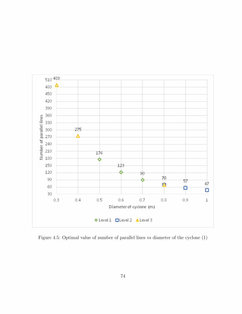
Figure 4.5: Optimal value of number of parallel lines vs diameter of the cyclone (1)

74

Figure 4.6: Optimal value of number of parallel lines vs diameter of the cyclone (2)

75

The maximum value of the overall efficiency of the cyclone arrangement that can be

attained for a certain upper bound of the cyclone diameter is shown in Figure 4.7. The

overall efficiency decreased nonlinearly as cyclone diameter increased with different slope

of each level (cyclone arrangement) being chosen. The relationship between the overall

efficiency and cyclone diameter in this optimization confirms the same relationship obtained

by Faulkner et al. [27], who studied the effects of cyclone diameter on the collection

efficiency of 1D3D cyclones. Moreover, a higher collection efficiency is accompanied by an

increase in value of the inlet velocity and pressure drop across the cyclone, resulting in a

higher total cost. Similar result were also reported by Gimbun et al. [41].

Figure 4.8 presents the relationship between the optimal value of the cyclone diameter

and the minimum total cost achieved from the optimization. From this figure, an increase

in the optimal value of Dp will result in a decrease in the total cost ctot. This is because

the operating cost is proportional to 1D2 and even though the capital cost is proportional to

diameter of the cyclone, a decreased value of the operating cost tends to be more dominant

than the capital cost in obtaining the optimum total cost.

76

Figure 4.7: Optimal value of the overall efficiency vs diameter of the cyclone

77

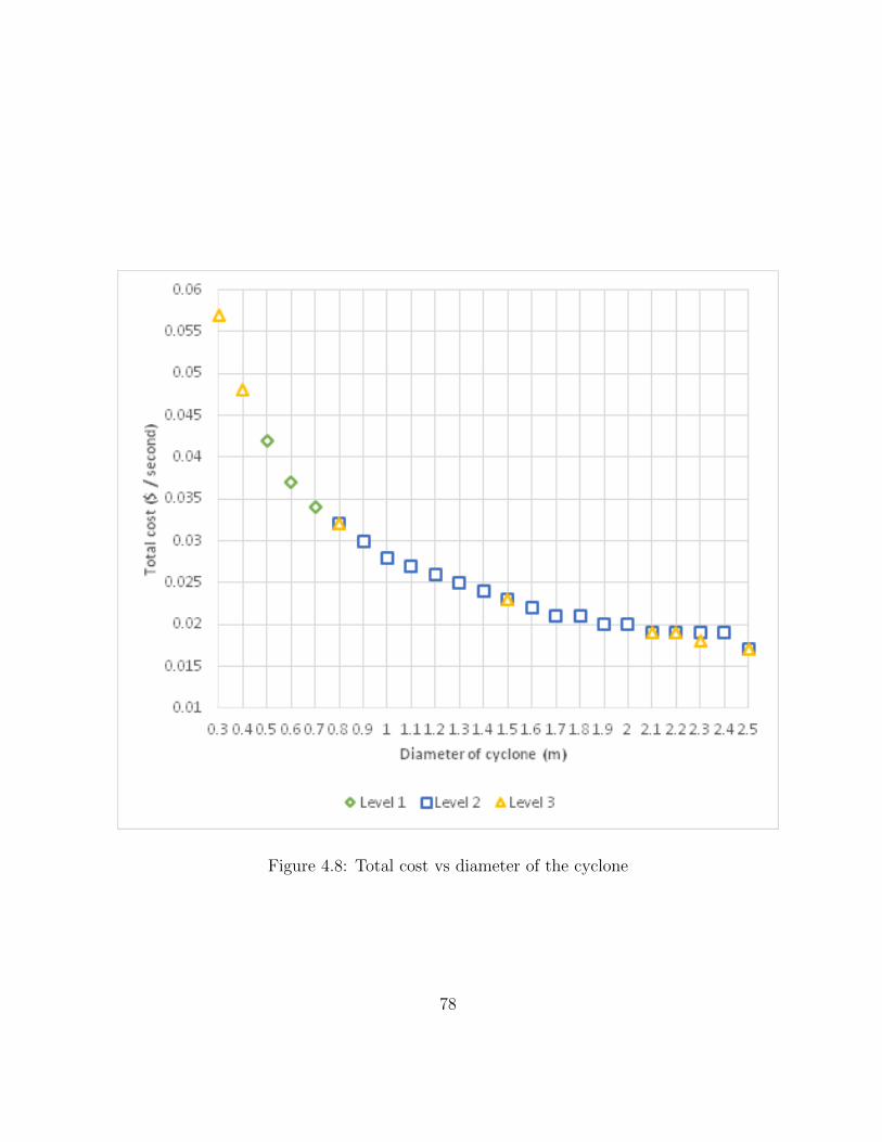
Figure 4.8: Total cost vs diameter of the cyclone

78

In addition, since the dimensions of the second cyclone would be the same as the first

cyclone, the optimum efficiency of the second cyclones would have a lower value than the

first cyclone. A lower value of the efficiency of the second cyclone compared to the first

cyclone can be explained theoretically wherein by keeping the dimensions of the second

cyclone to be similar to the first cyclone and as it is known that the calculation of the

diameter of the second cyclone will be affected by the overall efficiency of the first cyclone

(Eqs.(4.28-4.29)), the value of cut-size diameter of the second cyclone will increase to retain

the value of the cyclone diameter. Thus, as can be seen in Figure 4.4, a higher value of

the cut-size diameter will result in a lower value of the cyclone efficiency. So, the overall

efficiency of the second cyclone shall not be higher than the value of the overall efficiency

of the first cyclone. These results are found to be in line with the results reported by

Whitelock and Buser [118], who studied the performance of multiple (up to four) 1D3D

cyclones arranged in series.

It is interesting to observe from Figure 4.7 that there are only three from four levels

available that have been chosen by the model as the best arrangement for a certain value

of the decision variables Dp and Np. For instance, with the resultant value of the efficiency

more than 75 %, level 3 (1D3D+2D2D) is selected as the best cyclone arrangement for

Dp = 0.3 - 0.4 m, level 1 (1D3D+1D3D) for Dp = 0.5 m, and level 2 (2D2D+2D2D) for

Dp = 0.8 - 1.0 m. From the whole range, level 1 is available only when the value of Dp is

in the range between 0.5 - 0.7 m. Meanwhile, level 2 is found being more dominant than

the others in which it is selected as the best arrangement for a wide range value of the

optimum diameter of the cyclone (Dp = 0.8 m to 2.5 m).

At a certain point, there are two levels selected as the best arrangement with the same

Dp and Np. For example, the upper bound value of 0.8 m, 1.5 m, 2.1 m, 2.4 m, and 2.5 m

would result in two levels selected (i.e., level 2 and level 3) as the best arrangement with

the same optimum number of parallel lines at each Dp. Another result shows that, the

same two levels are selected as the best arrangement with the same Dp = 2.2 m, but with

different value of Np. The total costs associated with each levels (Figure 4.8) is found to be

having the same value. Based on these results, two different types of cyclone arrangement

79

can be selected at the same cost but with different efficiencies (Figure 4.7) where the overall

efficiency of cyclone arrangement on level 2 (2D2D+2D2D) is found higher than level 3

(1D3D+2D2D).

To further check the sensitivity of the decision variables to the optimal solutions, an

additional optimization was also performed by using all the three decision variables (N , Dp,

and ηov). This optimization is also intended to computationally investigate the effect of ηov

if the bound is changed. In this case, the lower bound of the overall cyclone efficiency (ηLov)

is set to have the initial value of 80 % and then increase in increments of 5 %. Meanwhile, a

priori bounds of NUp and DU

p are also selected. The optimal value of cyclone diameter and

number of parallel lines for a given constraint of decision variable ηov should lie within the

bounds. Otherwise, a higher value of the upper bound (DUp and NU

p ) should be applied.

The computational results of the optimization are shown in Table 4.15. The method

selects the lower bound of ηov as the optimal value. The sensitivity of ηov to the optimal

solutions obtained from this optimization are found to be in accordance with the numerical

findings from the previous study (Tables 4.5 - 4.14). For instance, as the cyclone diameter

decreased along with the optimal value of inlet cyclone remains constant at its upper

bound, the overall efficiency will increase. The optimal value of ηov = 90 % obtained in

this optimization is higher than the value of the previous optimization (ηov = 86.8 %).

It indicates that a higher ηov is attainable by changing its lower bound until the optimal

solution could be reached.

From Table 4.15, the model shows its consistency in selecting the cyclone arrangement

of 1D3D+2D2D (level 3) as the best arrangement to obtain the optimal value of overall

efficiency in the range of 80 % - 90 %. If these results are combined with the results given

in Tables 4.5 - 4.6 (for ηov > 80 %), it will complete the search for the optimal solution

of level 3 to attain the maximum value of overall efficiency as presented in Table 4.16.

However, the optimal solution for ηov = 90 % (Table 4.15) provides two levels as the best

arrangement, i.e., level 2 and 3. The cyclone arrangement of 2D2D+2D2D (level 2) will

have a lower optimum number of parallel lines even though its dimensions are bigger than

80

the cyclone arrangement of 1D3D+2D2D (level 3). Consequently, the total cost of the

cyclone arrangement of 2D2D+2D2D is lower than the 1D3D+2D2D, or in other words,

the cyclone arrangement of 2D2D+2D2D is more efficient in total cost.

DUp NU

p ηLov ηUov k Dp Np η1 η2 ηovt vip ∆p ctot

1 450 0.8 1 3 0.476 194 0.752 0.193 0.8 30 2186.78 0.043

1 450 0.85 1 3 0.344 373 0.813 0.2 0.85 30 2186.78 0.052

2 1000 0.9 1 3 0.226 861 0.875 0.202 0.9 30 2186.78 0.069

1 550 0.9 1 2 0.425 244 0.888 0.11 0.9 30 2186.78 0.046

Table 4.15: Optimization result using the decision variables N and ηov

k Dp Np η1 η2 ηovt vip ∆p ctot

3 0.476 194 0.752 0.193 0.8 30 2186.78 0.043

3 0.4 275 0.786 0.197 0.828 30 2186.718 0.048

3 0.344 373 0.813 0.2 0.85 30 2186.78 0.052

3 0.3 489 0.835 0.201 0.868 30 2186.718 0.057

3 0.226 861 0.875 0.202 0.9 30 2186.78 0.069

Table 4.16: Complete results for level 3 as the best arrangement and ηovt = 80 % - 90 %

The optimization results obtained from the present mathematical programming models

were also compared with the results from Ravi et al. [83], who studied a multi-objective

optimization of a set of N identical reverse-flow cyclone separators in parallel by using the

non-dominated sorting genetic algorithm (NSGA). Since they used nine decision variables

in the optimization, compared to three decision variables in the present study, not all results

would be presented. In particular, only the optimum solution of the number of parallel

cyclones, cyclone diameter, and the efficiency of the cyclone are used for comparison. Table

81

4.17 lists comparisons of the optimal solution of decision variables, i.e., number of cyclone,

diameter of the cyclone, and efficiency of the cyclone, where the results were evaluated using

the same input feed (Table 4.3) and the same range of dimensions ratio of the cyclones

(i.e., a0, b0, and De0). It should be noted that there is no table provided in Ravi et al. [83]

results, all the results presented in scatter charts instead. Hence, the values listed in Table

4.17 are rough estimated number from those charts provided.

Table 4.17: Comparison of the optimal solution of decision variables

The comparisons illustrated that the present study gave the lower number of parallel

cyclones for the same value of the efficiency of the cyclone. In addition, the optimum

efficiency of the cyclone that can be achieved from the present study (90 %) is slightly

higher than Ravi et al. [83]. Based on the above comparisons, it can be concluded that

the optimization of the cyclone arrangement in parallel-series using 1D3D and/or 2D2D

cyclones found to be a novel solution among other pollution control strategies to reduce

the pollution to the minimum level.

4.5 Chapter Summary

This chapter presented a MINLP (Mixed Integer Nonlinear Programming) model to find

the best cyclone arrangement with the optimal number and configuration / dimensions

82

of the cyclone from four combinations of 1D3D and 2D2D cyclones arranged in parallel-

series. The cyclone arrangement is optimized with respect to the minimum total cost

which includes the operating cost and capital cost. The proposed model is implemented

to handle a total flow rate of 165 m3/s of a stream to be processed in a paper mill.

The MINLP problem was carried out using DICOPT that runs under GAMS, while the

MILP master problem and NLP subproblem were solved using CPLEX and CONOPT 3,

respectively. Three decision variables (N , D, and ηov) were involved in selecting the best

cyclone arrangement from four levels available (1D3D+1D3D, 2D2D+2D2D, 1D3D+2D2D,

and 2D2D+1D3D). It was found that D is the important decision variable that led the

model to obtain the optimal solution. Different values used for the upper bound of D and

N results in three different cyclone arrangements selected as the optimal solution. The

sensitivity of the decision variables to the optimal solution is described as follows: the

overall efficiency of the cyclone as well as the optimal number of the cyclone will decrease

as the cyclone diameter increases, followed by a decrease in the total cost. As a result

of this study, the parallel-series cyclone arrangement of 2D2D+2D2D is found to be more

economical and efficient compared to the others.

83

Chapter 5

Conclusions and Recommendations

The use of multiple cyclones can be considered as one solution to the demands of obtaining

the best pollution control strategies to achieve a minimum level of pollution reduction. In

order to give the best solution in designing an optimum arrangement and dimensions of the

cyclone, there is a need to develop an effective mathematical programming combined with

the use of modern tools of optimization. A summary of the findings of new methods to the

solution of cyclone arrangement problems is presented in Section 5.1. Recommendations

for future work in this field are discussed in Section 5.2.

5.1 Conclusion

Mathematical programming models aimed at obtaining the best configuration of multi-

ple cyclone arrangement has been developed. The key idea of the present mathematical

programming model is to present the capability of General Algebraic Modeling System

(GAMS) software in solving multiple cyclone arrangement problems. Two mathematical

programming techniques are used to optimize different cyclone arrangement i.e., nonlinear

programming (NLP) model for 1D3D, 2D2D, and 1D2D cyclones in parallel or in series

and mixed integer nonlinear programming (MINLP) model for four combinations of 1D3D

84

and 2D2D cyclones arranged in parallel-series. The objective of all these models is to find

the optimal number and dimensions of cyclone arrangement with respect to the minimum

total cost including the operating cost and the capital cost.

The proposed model of nonlinear programming optimization of series and parallel cy-

clone arrangement is applied in NPK (Nitrogen, Phosphorus, and Potassium) fertilizer

plant. Different types of cyclones, in parallel or in series arrangements, result in different

optimal numbers of cyclones. Each type of cyclone (i.e., 1D3D, 2D2D, and 1D2D) has an

alternative that can be arranged either in parallel or in series configuration. The cyclone

diameter becomes a basic consideration because it determines the overall size of the cy-

clone, especially for the cyclone height. Therefore, if the available space is limited on the

field, it is advised to choose the small cyclone with a small number of the cyclone arrange-

ment. The 1D3D cyclones connected in parallel have the smallest diameter for the same

value of optimal number of cyclones (N = 3) compared with the other two. The 1D2D

cyclone in a series is more suitable to handle a given input feed of which it has the lowest

pressure drop with the smallest size of diameter (i.e., 2.5 m) compared to the others. In

addition, two cyclones in series is more likely to be operated than three cyclones because

the total cost of three cyclones in series is higher than the two cyclones.

A MINLP (Mixed Integer Nonlinear Programming) model to find the best cyclone

arrangement with the optimal number of cyclones and dimensions from four combinations

of 1D3D and 2D2D cyclones arranged in parallel-series has been successfully developed.

Three decision variables (N , D, and ηov) have a strong influence in selecting the best

cyclone arrangement from four levels available (1D3D+1D3D, 2D2D+2D2D, 1D3D+2D2D,

and 2D2D+1D3D). Different values used for the upper bound of D and N would result in

different cyclone arrangement selected as the optimal solution. The sensitivity results of

the decision variables to the optimal solution are found in line with the results obtained

from other researcher who studied in the same area by experimentally or computationally.

The optimum value of 90 % of the overall efficiency for a given feed with a high volume and

heavy loading of solid particles (Q = 165 m/s and ρp = 1600 kg/m3) can be attained either

by 1D3D+2D2D cyclones arrangement or 2D2D+2D2D cyclones arrangement in parallel-

85

series with different dimensions and number of the cyclone. The cyclone arrangement of

2D2D+2D2D in parallel-series is found to be the best arrangement with a higher efficiency

and a lower total cost compared to the others.

5.2 Recommendations

The research presented in this work can be extended further to increase its contribution to

the field of optimal multiple cyclone arrangement. Some of the recommendations for the

way forward of this research are discussed below.

• General Algebraic Modeling System (GAMS) software in solving multiple cyclone

arrangement problems in this work has proved its capability to handle a nonlin-

earity in multiple cyclone arrangement problem then produce an optimal solution

of the optimal number, dimensions, and the best cyclone arrangement. Although

this work has produce an optimal solution for cyclone arrangement problem, there

are several assumptions involved in the optimization. For example, since all the

equations used in this work derived from the time-of-flight model and no cut-size

diameter correction factor was found in the literature for its model, the correction

factor for equilibrium-orbit model (the model of Barth) was used in the cut-size di-

ameter equation. Therefore, an experiment in order to find a correction factor to

modify the theoretical cut-size diameter of time-of-flight model to quantify the effect

of PSD on the cut-size diameter calculation is recommended for future work.

• It is known that the efficiency of cyclone systems is a function of the particle size

distribution (PSD) of entrained dust to the cyclone. In this work, due to limitations

of available data in the literature, the PSD of the particles of the feed entered to the

second cyclone in series of all type of cyclones was assumed to be the same with the

experimental result of 1D3D+1D3D cyclones. Additional optimization using different

PSD data that enter to the second cyclone for other combinations of cyclones (i.e.,

86

1D3D+2D2D, 2D2D+2D2D, 2D2D+1D3D) and actual field tests are recommended

as part of the future work in this research.

• The study presented in this work made use of three types of cyclone, i.e., 1D3D,

2D2D, and 1D2D cyclone. Expanding the study to address the optimal solution of

multiple cyclone arrangement in parallel, series, and parallel-series using combina-

tions of a wide range type of the cyclone is recommended for future work.

• The optimization results using GAMS software which have been obtained in the

present work, allowing for more effective and optimal solution of a greater complexity

of the cyclone arrangement problem in the future.

87

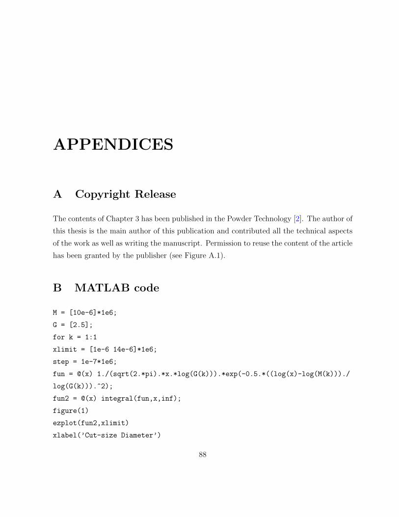
APPENDICES

A Copyright Release

The contents of Chapter 3 has been published in the Powder Technology [2]. The author of

this thesis is the main author of this publication and contributed all the technical aspects

of the work as well as writing the manuscript. Permission to reuse the content of the article

has been granted by the publisher (see Figure A.1).

B MATLAB code

M = [10e-6]*1e6;

G = [2.5];

for k = 1:1

xlimit = [1e-6 14e-6]*1e6;

step = 1e-7*1e6;

fun = @(x) 1./(sqrt(2.*pi).*x.*log(G(k))).*exp(-0.5.*((log(x)-log(M(k)))./

log(G(k))).^2);

fun2 = @(x) integral(fun,x,inf);

figure(1)

ezplot(fun2,xlimit)

xlabel(’Cut-size Diameter’)

88

ylabel(’Efficiency’)

grid on

hold all

j = 0;

end

-----------------------------------------

M = [3.7e-6]*1e6;

G = [2.5];

for k = 1:1

xlimit = [1e-7 10e-6]*1e6;

step = 1e-7*1e6;

fun = @(x) 1./(sqrt(2.*pi).*x.*log(G(k))).*exp(-0.5.*((log(x)-log(M(k)))./

log(G(k))).^2);

fun2 = @(x) integral(fun,x,inf);

figure(1)

ezplot(fun2,xlimit)

xlabel(’Cut-size Diameter’)

ylabel(’Efficiency’)

grid on

hold all

j = 0;

end

89

Figure A.1: License agreement copy from Elsevier to reuse content of article

90

References

[1] GAMS-CPLEX solver description.

[2] Sabah Ahmed Abdul-Wahab, Muhamad Fariz Failaka, Lena Ahmadi, Ali Elkamel,

and Kaan Yetilmezsoy. Nonlinear programming optimization of series and parallel

cyclone arrangement of npk fertilizer plants. Powder Technology, 264:203–215, 2014.

[3] R McK Alexander. Fundamentals of cyclone design and operation. Proc. Aus. Inst.

Min. Met. NS, 152(3):152–153, 1949.

[4] Ioannis P Androulakis, Costas D Maranas, and Christodoulos A Floudas. αbb: A

global optimization method for general constrained nonconvex problems. Journal of

Global Optimization, 7(4):337–363, 1995.

[5] A Avci and I Karagoz. Theoretical investigation of pressure losses in cyclone sep-

arators. International communications in heat and mass transfer, 28(1):107–117,

2001.

[6] W Barth. Design and layout of the cyclone separator on the basis of new investiga-

tions. Brenn. Warme Kraft, 8:1–9, 1956.

[7] Jaime Benıtez. Process engineering and design for air pollution control. Prentice

Hall, 1993.

91

[8] V Bhaskar, Santosh K Gupta, and Ajay K Ray. Applications of multiobjective

optimization in chemical engineering. Reviews in Chemical Engineering, 16(1):1–54,

2000.

[9] R Byron Bird, Warren E Stewart, and Edwin N Lightfoot. Transport phenomena.

John Wiley & Sons, 2007.

[10] Anthony J Buonicore and Wayne T Davis. Air pollution engineering manual. Van

Nostrand Reinhold, 1992.

[11] Joaquin Casal and Jose M Martinez-Benet. Better way to calculate cyclone pressure

drop. Chemical engineering, 90(2):99–100, 1983.

[12] Jianyi Chen and Mingxian Shi. A universal model to calculate cyclone pressure drop.

Powder technology, 171(3):184–191, 2007.

[13] Amy R Ciric and Deyao Gu. Synthesis of nonequilibrium reactive distillation pro-

cesses by minlp optimization. AIChE Journal, 40(9):1479–1487, 1994.

[14] Roland Clift, John R Grace, and Martin E Weber. Bubbles, drops, and particles.

Courier Corporation, 2005.

[15] EP Columbus. Series cyclone arrangements to reduce gin emissions. Transactions of

the ASAE (USA), 1993.

[16] JJ Derksen. Separation performance predictions of a stairmand high-efficiency cy-

clone. AIChE Journal, 49(6):1359–1371, 2003.

[17] John Dirgo and David Leith. Cyclone collection efficiency: comparison of experimen-

tal results with theoretical predictions. Aerosol Science and Technology, 4(4):401–

415, 1985.

[18] LCW Dixon. Global optima without convexity. Numerical Optimisation Centre,

Hatfield Polytechnic, 1977.

92

[19] LCW Dixon and GP Szego. The global optimization problem: an introduction.

Towards global optimization, 2:1–15, 1978.

[20] Arne Drud. GAMS-CONOPT solver description.

[21] MA Duran and IE Grossmann. A mixed-integer nonlinear programming algorithm

for process systems synthesis. AIChE journal, 32(4):592–606, 1986.

[22] Marco A Duran and Ignacio E Grossmann. An outer-approximation algorithm for

a class of mixed-integer nonlinear programs. Mathematical programming, 36(3):307–

339, 1986.

[23] Alexia A Economopoulou and Alexander P Economopoulos. Method for estimating

size-specific particulate emission inventories. Journal of environmental engineering,

127(12):1139–1148, 2001.

[24] Thomas GW Epperly and Ross E Swaney. Branch and bound for global nlp: New

bounding lp. Nonconvex Optimization and Its Applications, 9:1–36, 1996.

[25] Grossmann et al. GAMS-DICOPT solver description.

[26] WB Faulkner and BW Shaw. Efficiency and pressure drop of cyclones across a range

of inlet velocities. Applied engineering in agriculture, 22(1):155, 2006.

[27] William B Faulkner, Michael D Buser, Derek P Whitelock, and Bryan W Shaw.

Effects of cyclone diameter on performance of 1d3d cyclones: collection efficiency.

Transactions of the ASABE, 50(3):1053–1059, 2007.

[28] MW First. Cyclone dust collector design. In Am. Soc. Mech. Eng, volume 49, pages

127–132, 1949.

[29] Roger Fletcher and Sven Leyffer. Solving mixed integer nonlinear programs by outer

approximation. Mathematical programming, 66(1-3):327–349, 1994.

93

[30] CA Floudas, A Aggarwal, and AR Ciric. Global optimum search for nonconvex nlp

and minlp problems. Computers & Chemical Engineering, 13(10):1117–1132, 1989.

[31] CA Floudas and AR Ciric. Strategies for overcoming uncertainties in heat exchanger

network synthesis. Computers & Chemical Engineering, 13(10):1133–1152, 1989.

[32] CA Floudas and GE Paules. A mixed-integer nonlinear programming formulation

for the synthesis of heat-integrated distillation sequences. Computers & chemical

engineering, 12(6):531–546, 1988.

[33] CA Floudas and V Visweswaran. A global optimization algorithm (gop) for certain

classes of nonconvex nlpsi. theory. Computers & chemical engineering, 14(12):1397–

1417, 1990.

[34] Christodoulos A Floudas and Avanish Aggarwal. A decomposition strategy for global

optimum search in the pooling problem. ORSA Journal on Computing, 2(3):225–235,

1990.

[35] Christodoulos A Floudas and Vishy Visweswaran. Primal-relaxed dual global opti-

mization approach. Journal of Optimization Theory and Applications, 78(2):187–225,

1993.

[36] PA Funk, RW Clifford, and SE Hughs. Optimum entry velocity for modified 1d3d

cyclones. In ASAE Paper No. 994198. 1999.

[37] Arthur M Geoffrion. Generalized benders decomposition. Journal of optimization

theory and applications, 10(4):237–260, 1972.

[38] AM Gerrard and CJ Liddle. The optimal choice of multiple cyclones. Powder Tech-

nology, 13(2):251–254, 1976.

[39] MN Gillum and SE Hughs. Velocity effects on operating parameters of series cyclones.

Transactions of the ASAE, 26(2):606–609, 1983.

94

[40] MN Gillum, SE Hughs, and BM Armijo. Use of secondary cyclones for reducing gin

emissions. Transactions of the ASAE, 25(1):210–213, 1982.

[41] Jolius Gimbun, TG Chuah, Thomas SY Choong, and A Fakhru’l-Razi. A cfd study

on the prediction of cyclone collection efficiency. International Journal for Compu-

tational Methods in Engineering Science and Mechanics, 6(3):161–168, 2005.

[42] Jolius Gimbun, TG Chuah, A Fakhrul-Razi, and Thomas SY Choong. The influence

of temperature and inlet velocity on cyclone pressure drop: a cfd study. Chemical

Engineering and Processing: Process Intensification, 44(1):7–12, 2005.

[43] WD Griffiths and F Boysan. Computational fluid dynamics (cfd) and empirical

modelling of the performance of a number of cyclone samplers. Journal of Aerosol

Science, 27(2):281–304, 1996.

[44] Ignacio E Grossmann. Mixed-integer programming approach for the synthesis of in-

tegrated process flowsheets. Computers & chemical engineering, 9(5):463–482, 1985.

[45] Ignacio E Grossmann. Mixed-integer nonlinear programming techniques for the syn-

thesis of engineering systems. Research in Engineering Design, 1(3-4):205–228, 1990.

[46] Ignacio E Grossmann. Mixed-integer optimization techniques for algorithmic process

synthesis. Advances in Chemical Engineering, 23:171–246, 1996.

[47] Ignacio E Grossmann. Review of nonlinear mixed-integer and disjunctive program-

ming techniques. Optimization and Engineering, 3(3):227–252, 2002.

[48] Ignacio E Grossmann et al. Minlp optimization strategies and algorithms for process

synthesis. 1989.

[49] Ignacio E Grossmann and Zdravko Kravanja. Mixed-integer nonlinear programming

techniques for process systems engineering. Computers & Chemical Engineering,

19:189–204, 1995.

95

[50] Ignacio E Grossmann and Jorge Santibanez. Applications of mixed-integer linear

programming in process synthesis. Computers & Chemical Engineering, 4(4):205–

214, 1980.

[51] Omprakash K Gupta and A Ravindran. Branch and bound experiments in convex

nonlinear integer programming. Management science, 31(12):1533–1546, 1985.

[52] AJ Hoekstra, JJ Derksen, and HEA Van Den Akker. An experimental and numerical

study of turbulent swirling flow in gas cyclones. Chemical Engineering Science,

54(13):2055–2065, 1999.

[53] Arjen Jacco Hoekstra. Gas flow field and collection efficiency of cyclone separators.

PhD thesis, TU Delft, Delft University of Technology, 2000.

[54] AC Hoffmann, M De Groot, W Peng, HWA Dries, and J Kater. Advantages and

risks in increasing cyclone separator length. AIChE journal, 47(11):2452–2460, 2001.

[55] AC Hoffmann and LE Stein. Gas cyclones and swirl tubes: Principles. Design and

Operation, 2nd Edition Springer, 2008.

[56] Reiner Horst and Hoang Tuy. Global optimization: Deterministic approaches.

Springer Science & Business Media, 2013.

[57] Donna Lee Iozia and David Leith. Effect of cyclone dimensions on gas flow pattern

and collection efficiency. Aerosol Science and Technology, 10(3):491–500, 1989.

[58] B Kalen and FA Zenz. Theoretical-empirical approach to saltation velocity in cyclone

design. In AIChE Symposium Series, volume 70, pages 388–396, 1974.

[59] Irfan Karagoz and Atakan Avci. Modelling of the pressure drop in tangential inlet

cyclone separators. Aerosol Science and Technology, 39(9):857–865, 2005.

[60] LC Kenny and RA Gussman. A direct approach to the design of cyclones for aerosol-

monitoring applications. Journal of aerosol science, 31(12):1407–1420, 2000.

96

[61] Wolfgang H KOCH and William LICHT. New design approach boosts cyclone effi-

ciency. Chemical engineering, 84(24):80–88, 1977.

[62] Gary R Kocis and Ignacio E Grossmann. Relaxation strategy for the structural

optimization of process flow sheets. Industrial & engineering chemistry research,

26(9):1869–1880, 1987.

[63] Gary R Kocis and Ignacio E Grossmann. Global optimization of nonconvex mixed-

integer nonlinear programming (minlp) problems in process synthesis. Industrial &

Engineering Chemistry Research, 27(8):1407–1421, 1988.

[64] E Kondili, CC Pantelides, and RWH Sargent. A general algorithm for short-term

scheduling of batch operationsi. milp formulation. Computers & Chemical Engineer-

ing, 17(2):211–227, 1993.

[65] Zdravko Kravanja and Ignacio E Grossmann. Prosynan minlp process synthesizer.

Computers & chemical engineering, 14(12):1363–1378, 1990.

[66] Hong Ming Ku and Iftekhar A Karimi. Scheduling in serial multiproduct batch

processes with finite interstage storage: mixed integer linear program formulation.

Industrial & engineering chemistry research, 27(10):1840–1848, 1988.

[67] Ashwani Kumar and Angelo Lucia. Separation process optimization calculations.

Applied numerical mathematics, 3(5):409–425, 1987.

[68] David Leith and William Licht. The collection efficiency of cyclone type particle

collectors: a new theoretical approach. In AIChE Symp. Ser, volume 68, pages

196–206, 1972.

[69] KS Lim, HS Kim, and KW Lee. Characteristics of the collection efficiency for a

cyclone with different vortex finder shapes. Journal of Aerosol science, 35(6):743–

754, 2004.

97

[70] A Lucia, J Xu, and KM Layn. Nonconvex process optimization. Computers &

chemical engineering, 20(12):1375–1398, 1996.

[71] VASILIOS MANOUSIOUTHAKIS and DENNIS SOURLAS. A global optimization

approach to rationally constrained rational programming. Chemical Engineering

Communications, 115(1):127–147, 1992.

[72] JM Martinez-Benet and J Casal. Optimization of parallel cyclones. Powder technol-

ogy, 38(3):217–221, 1984.

[73] A Mauderli and DWT Rippin. Production planning and scheduling for multi-purpose

batch chemical plants. Computers & Chemical Engineering, 3(1):199–206, 1979.

[74] Soterios A Papoulias and Ignacio E Grossmann. A structural optimization approach

in process synthesisiii: total processing systems. Computers & chemical engineering,

7(6):723–734, 1983.

[75] CB Parnell Jr and DD Davis. Predicted effects of the use of new cyclone designs on

agricultural processing particulate emissions. In ASAE Southwest Region Meeting.

St. Joseph, Mich.: ASAE, 1979.

[76] W Peng, AC Hoffmann, PJAJ Boot, A Udding, HWA Dries, A Ekker, and J Kater.

Flow pattern in reverse-flow centrifugal separators. Powder Technology, 127(3):212–

222, 2002.

[77] F Pettersson and T Westerlund. Global optimization of pump configurations using

binary separable programming. Computers & chemical engineering, 21(5):521–529,

1997.

[78] JM Pinto and IE Grossmann. Optimal cyclic scheduling of multistage continuous

multiproduct plants. Computers & Chemical Engineering, 18(9):797–816, 1994.

98

[79] Jose M Pinto and Ignacio E Grossmann. A continuous time mixed integer linear

programming model for short term scheduling of multistage batch plants. Industrial

& Engineering Chemistry Research, 34(9):3037–3051, 1995.

[80] Ignacio Quesada and Ignacio E Grossmann. An lp/nlp based branch and bound algo-

rithm for convex minlp optimization problems. Computers & chemical engineering,

16(10):937–947, 1992.

[81] Ignacio Quesada and Ignacio E Grossmann. A global optimization algorithm for

linear fractional and bilinear programs. Journal of Global Optimization, 6(1):39–76,

1995.

[82] G Ramachandran, David Leith, John Dirgo, and Henry Feldman. Cyclone opti-

mization based on a new empirical model for pressure drop. Aerosol Science and

Technology, 15(2):135–148, 1991.

[83] G Ravi, Santosh K Gupta, and MB Ray. Multiobjective optimization of cyclone

separators using genetic algorithm. Industrial & engineering chemistry research,

39(11):4272–4286, 2000.

[84] Steven H Rich and George J Prokopakis. Scheduling and sequencing of batch oper-

ations in a multipurpose plant. Industrial & Engineering Chemistry Process Design

and Development, 25(4):979–988, 1986.

[85] K Rietema. Het mechanisme van de afscheiding van fijnverdeelde stoffen in cyclonen.

De Ingenieur, 71:39, 1959.

[86] Richard E Rosenthal. Gams–a user’s guide. 2004.

[87] P Rosin, E Rammler, and W Intelmann. Principles and limits of cyclone dust removal.

Zeit. Ver. Deutscher Ing, 76:433–437, 1932.

99

[88] Hong S Ryoo and Nikolaos V Sahinidis. Global optimization of nonconvex nlps and

minlps with applications in process design. Computers & Chemical Engineering,

19(5):551–566, 1995.

[89] Hong S Ryoo and Nikolaos V Sahinidis. A branch-and-reduce approach to global

optimization. Journal of Global Optimization, 8(2):107–138, 1996.

[90] NV Sahinidis and Ignacio E Grossmann. Minlp model for cyclic multiproduct schedul-

ing on continuous parallel lines. Computers & chemical engineering, 15(2):85–103,

1991.

[91] RWH Sargent and K Gaminibandara. Optimum design of plate distillation columns.

Optimization in action, pages 267–314, 1976.

[92] HI Shaban, A Elkamel, and R Gharbi. An optimization model for air pollution

control decision making. Environmental Modelling & Software, 12(1):51–58, 1997.

[93] N Shah, CC Pantelides, and RWH Sargent. A general algorithm for short-term

scheduling of batch operationsii. computational issues. Computers & Chemical En-

gineering, 17(2):229–244, 1993.

[94] CB Shepherd and CE Lapple. Air pollution control: a design approach. Cyclones,

second ed., Woveland Press Inc., Illinois, pages 127–139, 1939.

[95] CB Shephered and CE Lapple. Flow pattern and pressure drop in cyclone dust

collectors. Industrial & Engineering Chemistry, 31(8):972–984, 1939.

[96] S Simpson and CB Parnell Jr. New low-pressure cyclone design for cotton gins. In

Proc. 1995 Beltwide Cotton Production Conferences, pages 680–687, 1995.

[97] R.K. Sinnott. Chemical Engineering Design. Elsevier Butterworth-Heinemann, 2005.

[98] Edward MB Smith and Constantinos C Pantelides. Global optimisation of gen-

eral process models. In Global optimization in engineering design, pages 355–386.

Springer, 1996.

100

[99] Robin M Smith. Chemical process: design and integration. John Wiley & Sons, 2005.

[100] Giulio Solero and Aldo Coghe. Experimental fluid dynamic characterization of a

cyclone chamber. Experimental thermal and fluid science, 27(1):87–96, 2002.

[101] C J Stairmand. The design and performance of cyclone separators. Trans. Inst.

Chem. Eng, 29:356–383, 1951.

[102] George Stephanopoulos and Arthur W Westerberg. The use of hestenes’ method

of multipliers to resolve dual gaps in engineering system optimization. Journal of

Optimization Theory and Applications, 15(3):285–309, 1975.

[103] Prabhata K Swamee, Nitin Aggarwal, and Kuldeep Bhobhiya. Optimum design of

cyclone separator. AIChE journal, 55(9):2279–2283, 2009.

[104] RE Swaney. Global solution of algebraic nonlinear programs. In AIChE Annual

Meeting, Chicago, IL, 1990.

[105] Gifford H Symonds. Linear programming: the solution of refinery problems. Esso

Standard Oil Company, 1955.

[106] Athanasios G Tsirukis, Savoula Papageorgaki, and Gintaras V Reklaitis. Schedul-

ing of multipurpose batch chemical plants with resource constraints. Industrial &

engineering chemistry research, 32(12):3037–3050, 1993.

[107] R Vaidyanathan and M El-Halwagi. Global optimization of nonconvex nonlinear

programs via interval analysis. Computers & Chemical Engineering, 18(10):889–897,

1994.

[108] Jagadisan Viswanathan and Ignacio E Grossmann. A combined penalty function

and outer-approximation method for minlp optimization. Computers & Chemical

Engineering, 14(7):769–782, 1990.

101

[109] Jagadisan Viswanathan and Ignacio E Grossmann. An alternate minlp model for

finding the number of trays required for a specified separation objective. Computers

& chemical engineering, 17(9):949–955, 1993.

[110] Jagadisan Viswanathan and Ignacio E Grossmann. Optimal feed locations and num-

ber of trays for distillation columns with multiple feeds. Industrial & engineering

chemistry research, 32(11):2942–2949, 1993.

[111] L Wang, CB Parnell, BW Shaw, and RE Lacey. Analysis of cyclone collection ef-

ficiency. In Proceedings of 2003 ASAE Annual International Meeting, Las Vegas,

Paper, volume 34114, 2003.

[112] L Wang, CB Parnell, BW Shaw, and RE Lacey. A theoretical approach for predicting

number of turns and cyclone pressure drop. Transactions of the ASABE, 49(2):491–

503, 2006.

[113] Lingjuan Wang, Calvin B Parnell, and Bryan W Shaw. Performance characteristics

of cyclones in cotton-gin dust removal. Agricultural Engineering International: CIGR

EJournal., 2002.

[114] Lingjuan Wang, Calvin B Parnell, and Bryan W Shaw. Study of the cyclone fractional

efficiency curves. Agricultural Engineering International: CIGR EJournal., 2002.

[115] Lingjuan Wang, CB Parnell, and Bryan W Shaw. 1d2d, 1d3d, 2d2d cyclone fractional

efficiency curves for fine dust. In Proc. 2000 Beltwide Cotton Production Conferences,

2000.

[116] Tapio Westerlund and Frank Pettersson. A cutting plane method for solving convex

MINLP problems. Abo Akademi, 1994.

[117] Tapio Westerlund, Frank Pettersson, and Ignacio E Grossmann. Optimization

of pump configurations as a minlp problem. Computers & chemical engineering,

18(9):845–858, 1994.

102

[118] DP Whitelock and MD Buser. Multiple series cyclones for high particulate matter

concentrations. Applied engineering in agriculture, 23(2):131, 2007.

[119] Rongbiao Xiang, SH Park, and KW Lee. Effects of cone dimension on cyclone

performance. Journal of Aerosol Science, 32(4):549–561, 2001.

[120] Wen-ching Yang. Handbook of fluidization and fluid-particle systems. CRC press,

2003.

[121] Kaan Yetilmezsoy. Optimisation using prediction models: air cyclones’ body diame-

ter/pressure drop. Filtration & Separation, 42(10):32–35, 2005.

[122] Kaan Yetilmezsoy. Determination of optimum body diameter of air cyclones using

a new empirical model and a neural network approach. Environmental engineering

science, 23(4):680–690, 2006.

[123] BINGTAO Zhao. A theoretical approach to pressure drop across cyclone separators.

Chemical engineering & technology, 27(10):1105–1108, 2004.

103

superstructure optimization of multiple cyclone arrangements

Documents