sunflower sea star ( pycnopodia helianthoides
TRANSCRIPT
THE IUCN RED LIST OF THREATENED SPECIES™
Sunflower Sea Star (Pycnopodia helianthoides)
Red List Category: Critically Endangered
Year Published: 2020
Date Assessed: 26 August 2020
Date Reviewed: 31 August 2020
Assessors:
Sarah A. Gravem*, Oregon State University;
Walter N. Heady, The Nature Conservancy;
Vienna R. Saccomanno, The Nature Conservancy;
Kristen F. Alvstad, Oregon State University;
Alyssa L.M. Gehman, Hakai Institute;
Taylor N. Frierson, Washington Department of Fish and Wildlife;
Sara L. Hamilton*, Oregon State University.
* co-first-authors who contributed equally to the assessment
Reviewers
Gina Ralph, International Union for the Conservation of Nature;
Melissa Miner, University of California Santa Cruz and MARINe;
Pete Raimondi, University of California Santa Cruz and PISCO;
Steve Lonhart, Monterey Bay National Marine Sanctuary, NOAA.
Compilers
Rodrigo Beas-Luna, Universidad Autónoma de Baja California;
Joseph Gaydos, SeaDoc Society, UC Davis Karen C. Drayer Wildlife Health Center;
Drew Harvell, Cornell University and Friday Harbor Labs, University of Washington;
Erin Meyer, Seattle Aquarium.
Contributors
John Aschoff, Lindsay Aylesworth, Tristan Blaine, Jenn Burt, Jenn Caselle, Henry Carson, Mark Carr, Ryan Cloutier, Mike Dawson, Eduardo Diaz, David Duggins, Norah Eddy, George Esslinger, Fiona Francis, Jan Freiwald, Aaron Galloway, Katie Gavenus, Donna Gibbs, Josh Havelind, Jason Hodin, Elisabeth Hunt, Stephen Jewett, Christy Juhasz, Corinne Kane, Aimee Keller, Brenda Konar, Kristy Kroeker, Andy Lauermann,
Julio Lorda, Dan Malone, Scott Marion, Gabriela Montaño, Fiorenza Micheli, Tim Miller-Morgan, Melissa Neuman, Andrea Paz Lacavex, Michael Prall, Laura Rogers-Bennett, Nancy Roberson, Dirk Rosen, Anne Salomon, Jessica Schultz, Lauren Schiebelhut, Ole Shelton, Christy Semmens, Jorge Torre, Guillermo Torres-Moye, Nancy Treneman, Jane Watson, Ben Weitzman, and Greg Williams.
Institutional Contributions
The Nature Conservancy; The Kitasoo/Xai'xais Nation; The Heiltsuk Nation; The Wuikinuxv Nation; The Nuxalk Nation; The Haida Nation; iNaturalist; Glacier Bay National Park and Preserve; Gulf Watch Alaska; National Park Service Southwest Alaska; Olympic Coast National Marine Sanctuary; Parks Canada; Birch Aquarium at Scripps Institute of Oceanography; Aquarium and Rainforest at Moody Gardens; Aquarium du Quebec; Shedd Aquarium; Oregon Coast Aquarium; Rotterdam Zoo.
Acknowledgements
Funding for this assessment was provided by The Nature Conservancy. In addition to the contributors listed above, many institutions generously shared data with us for this project, which would have been impossible without their support. We would like to thank: The Alaska Fisheries Science Center, the Alaska Department of Fish and Game, the California Department of Fish and Wildlife, the Center for Alaskan Coastal Studies, the Central Coast Indigenous Resource Alliance, including the Kitasoo/Xai’xais Nation, Heiltsuk Nation, Wuikinuxv Nation, and Nuxalk Nation, Communidad y Biodiversidad, Glacier Bay National Park, Gulf Watch Alaska, the Hakai Institute, iNaturalist, Monterey Bay National Marine Sanctuary, the Multi-Agency Rocky Intertidal Network, National Park Service Southwest Alaska, NOAA’s National Marine Fisheries Science Center, Ocean Wise, the Vancouver Aquarium, the Olympic Coast National Marine Sanctuary, the Oregon Department of Fish and Wildlife, the Partnership for the Interdisciplinary Studies of Coastal Oceans, Reef Check, the Reef Environmental Education Foundation, Simon Fraser University, Universidad Autónoma de Baja California, University of Alaska - Fairbanks, University of California - Santa Cruz, USGS Alaska Science Center, Vancouver Island University, and the Washington Department of Fish and Wildlife for supporting initial data collection and sharing data for this project. Additionally, we thank The Council for the Haida Nation, Parks Canada, the Heiltsuk Nation, Kitasoo/Xai’xias Nation, Nuxalk Nation, and the Wuikinuxv Nation, Jenn Burt, Kyle Demes, Margot Hessing-Lewis, Brit Keeling, Lynn Lee, Hannah Stewart, and Rowan Trebilco for their part in the collection of Haida Gwaii and British Columbia data. Thanks to Andy Lamb and Charlie Gibbs for their contributions to the Ocean Wise data. Finally, we greatly appreciate the Seattle Aquarium, Birch Aquarium at Scripps Institute, the Aquarium & Rainforest at Moody Gardens, Aquarium du Quebec, Shedd Aquarium, Oregon Coast Aquarium, and the Rotterdam Zoo for sharing records of the Pycnopodia in their care.
Citation
Gravem, S.A., W.N. Heady, V.R. Saccomanno, K.F. Alvstad, A.L.M. Gehman, T.N. Frierson and S.L. Hamilton. 2021. Pycnopodia helianthoides. IUCN Red List of Threatened Species 2021.
Pycnopodia Populations in the Literature
Historical abundance
Literature on Pycnopodia helianthoides abundance before the 2013-2017 sea star wasting syndrome (SSWS) outbreak suggests that it was common throughout its range, with higher densities from the Salish Sea to the Aleutian Islands, Alaska. In the Gulf of Alaska, Konar et al. (2019) assessed rocky intertidal populations starting in 2012 and showed that it was common toward the northwest part of its range in the Katmai National Park and Preserve near Kodiak Island, Alaska (0.038 m-2 in 2012 and 0.048 m-2 in 2016, respectively, both before the local outbreak in 2016). Moving east along the Gulf of Alaska, they were less common in Kachemak Bay in the Cook Inlet (<0.005 m-2), fairly common in the Kenai Fjords National Park (~0.075/m-2), and quite common in western Prince William Sound (average 0.233/m-2) (Konar et al. 2019). In subtidal rocky reefs near Torch Bay, southeast Alaska, densities were high (0.09 ± 0.055 m-2) in the 1980s (Duggins 1983). In subtidal rocky reefs along the central coast of British Columbia, Pycnopodia biomass ranged from 0.57 to 0.93 kg/10 m2 in 2010‒2014 (Harvell et al. 2019). In Howe Sound, near Vancouver, British Columbia, densities were high at 0.43 ± 0.76 m-2 in 2009–2010 before the SSWS outbreak (Schultz et al. 2016). Montecino-LaTorre et al. (2016) found that Pycnopodia abundance averaged 6‒14 individuals per roving diver survey throughout much of the Salish Sea from 2006‒2013. In deep water habitats off the coasts of Washington, Oregon, and California 2004‒2014 pre-outbreak biomass averaged 3.11, 1.73, and 2.78 kg/10 ha, respectively (Harvell et al. 2019). Along the north and central California coastline, average population densities were 0.01‒0.12 m-2 prior to 2013 (Rogers-Bennett and Catton 2019). The oldest density records come from kelp forests near Monterey, California where densities were 0.03 per m-2 in 1980‒81 (Herrlinger 1983). Populations in the Channel Islands off Southern California have been studied extensively, and from 1982‒2014 densities ranged from 0‒0.25 m-2 (Bonaviri et al. 2017), from 1996‒1998 they were 0‒0.02 m-2 (Eckert 2007), from 2003‒2007 they were 0‒0.07 m-2 (Rassweiler et al. 2010), and from 2010‒2012 they were ~0.10‒0.14 m-2 (Eisaguirre et al. 2020).
SSWS-related declines in the literature
The outbreak of SSWS that began in 2013 resulted in high mortality and precipitous declines of Pycnopodia in shallow and deep waters throughout most of its range. Harvell et al. (2019) is the most spatially comprehensive analysis published, and shows severe declines coincident with the 2013‒2017 SSWS outbreak. In deep-water trawl surveys, they detected a 100% decline in Oregon and California (from an average of 1.73 kg/10 ha and 2.78 kg/10 ha from 2004‒2012, respectively, to none seen in 2015‒2016) and a 99.2% decline in Washington (from an average of 3.11 kg/10 ha in 2004‒2012 to 0.02 kg/10 ha in 2015-2016). In 2016, no Pycnopodia individuals were collected across the 1,264 ha area covered by 692 trawl surveys. Harvell et al. (2019) also showed similar dramatic declines in shallow subtidal populations from California to Alaska. Local and regional studies also documented declines due to SSWS. In the Gulf of Alaska, Konar et al. (2019) showed a 67‒94% decline in density of Pycnopodia in rocky intertidal habitats in the Gulf of Alaska coincident with the outbreak. In British Columbia, Burt et al. (2018) detected a decline of up to ~92% in Pycnopodia biomass on subtidal rocky reefs and Schultz et al. (2016) recorded an 86% decline in Pycnopodia densities in Howe Sound between 2009/2010 and 2015 (from [Mean ± SD] 430,000 ± 760,000 km-2
to 60,000 ± 220,000 km-2). In the Salish Sea, Montecino-LaTorre et al. (2016) showed divers averaged only 0‒3 sunflower star sightings per dive after the outbreak compared to 6‒14 before.
The most severe declines occurred along the outer coastline of the contiguous United States and Baja California, Mexico. During extensive surveys along the northern and central California coastlines, the California Department of Fish and Wildlife detected one Pycnopodia in 2014‒2015 and none in 2016–2019 (Rogers-Bennett and Catton 2019). Pycnopodia also appeared to be locally extinct in California’s Channel Islands, where none were found from 2014‒2017 (Eisaguirre et al. 2020). Because Pycnopodia is a broadcast spawner that does not appear to migrate to find mates, there is substantial concern that these sparse populations will neither successfully fertilize eggs during spawning nor see successful juvenile recruitment in the near future.
Population Data and Methods for IUCN Assessment
Data
Twenty-nine research groups from Canada, the United States, Mexico and First Nations shared 31 datasets containing field surveys of Pycnopodia for this effort (Fig. 1 and Table 1). The data included 61,043 surveys spanning 1967 to 2020 (Fig. 1b). We utilized multiple types of surveys including trawls, ROV Dives, SCUBA dives, intertidal surveys, and community science observations. They ranged from presence-only identifications by community scientists (e.g., iNaturalist) to quantitative estimates of density, size, and disease presence (e.g., Hakai Institute, Simon Fraser University-Salomon). We compiled all observations into a standardized format and included at minimum the latitude and longitude, date, depth, area surveyed, and Pycnopodia count. When datasets contained more than one survey on a site and date (e.g., multiple transects at the same location), we summed the count of Pycnopodia and the area searched, and averaged the latitude and longitude (if necessary). To determine densities, we divided the total count by the total area searched for each site and date. We then re-assigned presence and absence as 1 and 0, respectively, so that extent of occurrence and area of occupancy maps would reflect whether Pycnopodia was detected at a given site and date.
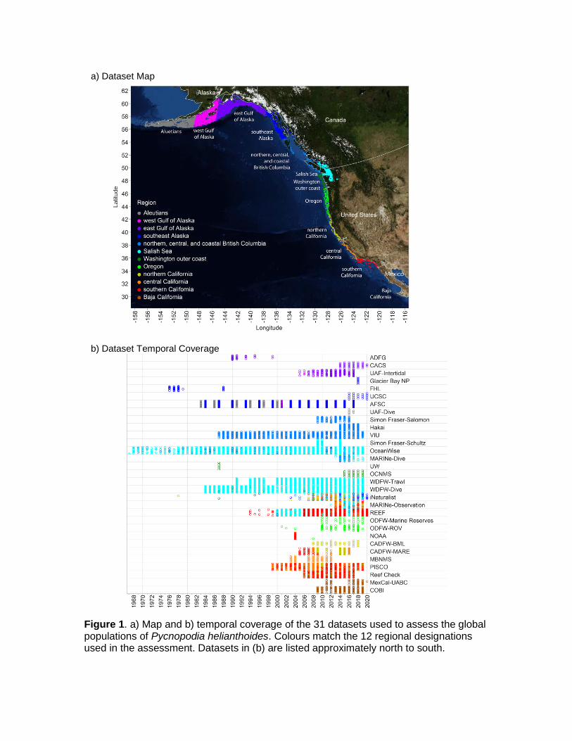
Figure 1. a) Map and b) temporal coverage of the 31 datasets used to assess the global populations of Pycnopodia helianthoides. Colours match the 12 regional designations used in the assessment. Datasets in (b) are listed approximately north to south.
b) Dataset Temporal Coverage
a) Dataset Map
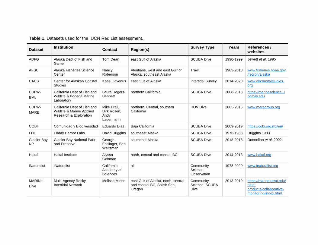
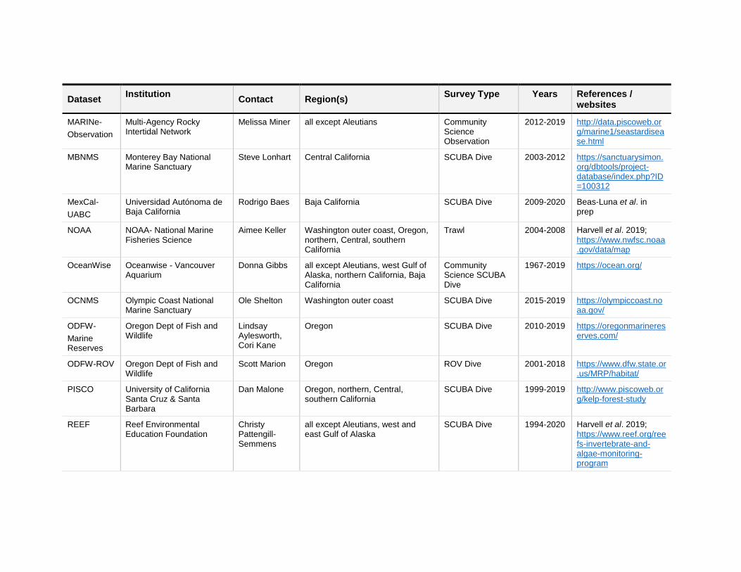
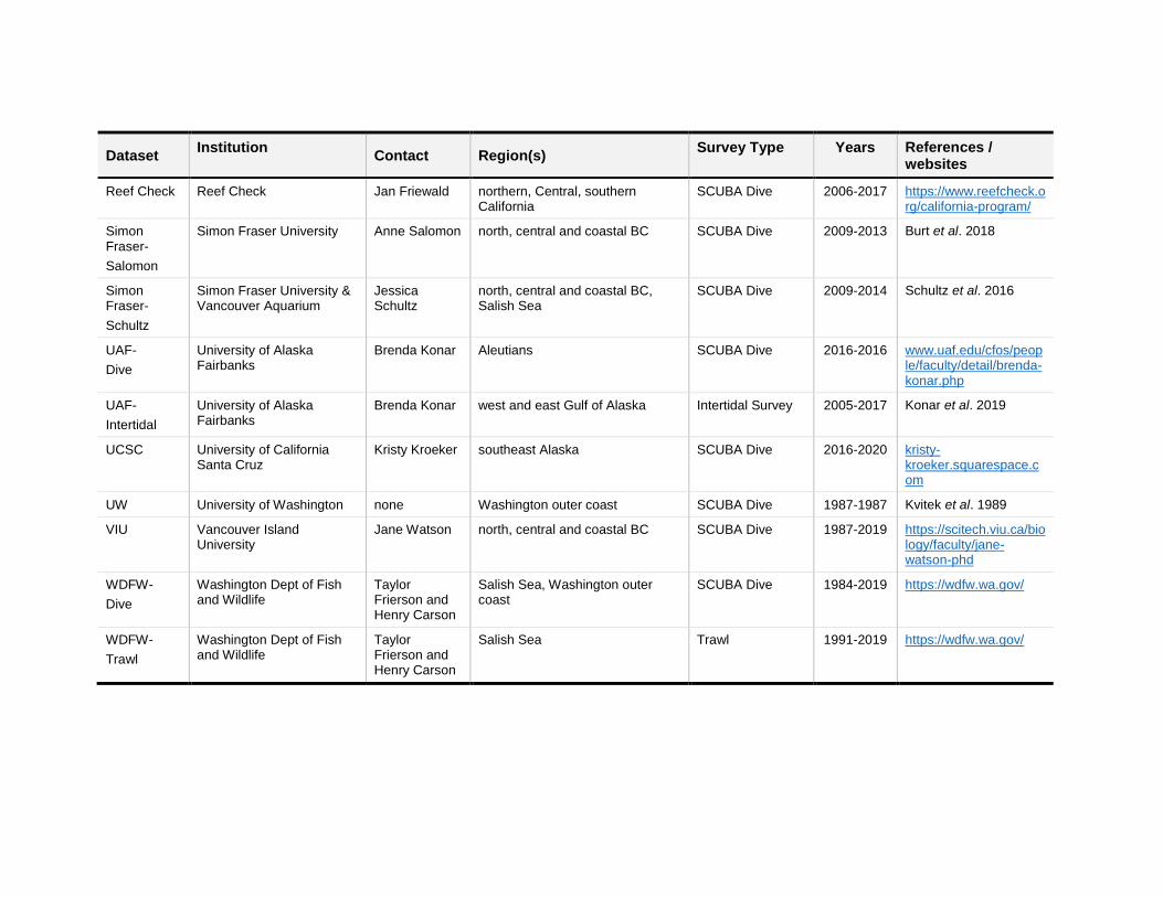
Table 1. Datasets used for the IUCN Red List assessment.
Dataset Institution
Contact Region(s) Survey Type Years References /
websites
ADFG Alaska Dept of Fish and Game
Tom Dean east Gulf of Alaska SCUBA Dive 1990-1999 Jewett et al. 1995
AFSC Alaska Fisheries Science Center
Nancy Roberson
Aleutians, west and east Gulf of Alaska, southeast Alaska
Trawl 1983-2018 www.fisheries.noaa.gov/region/alaska
CACS Center for Alaskan Coastal Studies
Katie Gavenus east Gulf of Alaska Intertidal Survey 2014-2020 www.akcoastalstudies.org
CDFW-
BML
California Dept of Fish and Wildlife & Bodega Marine Laboratory
Laura Rogers-Bennett
northern California SCUBA Dive 2008-2018 https://marinescience.ucdavis.edu
CDFW-
MARE
California Dept of Fish and Wildlife & Marine Applied Research & Exploration
Mike Prall, Dirk Rosen, Andy Lauermann
northern, Central, southern California
ROV Dive 2005-2016 www.maregroup.org
COBI Comunidad y Biodiversidad Eduardo Diaz Baja California SCUBA Dive 2009-2019 https://cobi.org.mx/en/
FHL Friday Harbor Labs David Duggins southeast Alaska SCUBA Dive 1976-1988 Duggins 1983
Glacier Bay NP
Glacier Bay National Park and Preserve
George Esslinger, Ben Weitzman
southeast Alaska SCUBA Dive 2018-2018 Donnellan et al. 2002
Hakai Hakai Institute Alyssa Gehman
north, central and coastal BC SCUBA Dive 2014-2018 www.hakai.org
iNaturalist iNaturalist California Academy of Sciences
all Community Science Observation
1978-2020 www.inaturalist.org
MARINe-
Dive
Multi-Agency Rocky Intertidal Network
Melissa Miner east Gulf of Alaska, north, central and coastal BC, Salish Sea, Oregon
Community Science; SCUBA Dive
2013-2019 https://marine.ucsc.edu/data-products/collaborative-monitoring/index.html
Dataset Institution
Contact Region(s) Survey Type Years References /
websites
MARINe-
Observation
Multi-Agency Rocky Intertidal Network
Melissa Miner all except Aleutians Community Science Observation
2012-2019 http://data.piscoweb.org/marine1/seastardisease.html
MBNMS Monterey Bay National Marine Sanctuary
Steve Lonhart Central California SCUBA Dive 2003-2012 https://sanctuarysimon.org/dbtools/project-database/index.php?ID=100312
MexCal-
UABC
Universidad Autónoma de Baja California
Rodrigo Baes Baja California SCUBA Dive 2009-2020 Beas-Luna et al. in prep
NOAA NOAA- National Marine Fisheries Science
Aimee Keller Washington outer coast, Oregon, northern, Central, southern California
Trawl 2004-2008 Harvell et al. 2019;
https://www.nwfsc.noaa.gov/data/map
OceanWise Oceanwise - Vancouver Aquarium
Donna Gibbs all except Aleutians, west Gulf of Alaska, northern California, Baja California
Community Science SCUBA Dive
1967-2019 https://ocean.org/
OCNMS Olympic Coast National Marine Sanctuary
Ole Shelton Washington outer coast SCUBA Dive 2015-2019 https://olympiccoast.noaa.gov/
ODFW-
Marine Reserves
Oregon Dept of Fish and Wildlife
Lindsay Aylesworth, Cori Kane
Oregon SCUBA Dive 2010-2019 https://oregonmarinereserves.com/
ODFW-ROV Oregon Dept of Fish and Wildlife
Scott Marion Oregon ROV Dive 2001-2018 https://www.dfw.state.or.us/MRP/habitat/
PISCO University of California Santa Cruz & Santa Barbara
Dan Malone Oregon, northern, Central, southern California
SCUBA Dive 1999-2019 http://www.piscoweb.org/kelp-forest-study
REEF Reef Environmental Education Foundation
Christy Pattengill-Semmens
all except Aleutians, west and east Gulf of Alaska
SCUBA Dive 1994-2020 Harvell et al. 2019; https://www.reef.org/reefs-invertebrate-and-algae-monitoring-program
Dataset Institution
Contact Region(s) Survey Type Years References /
websites
Reef Check Reef Check Jan Friewald northern, Central, southern California
SCUBA Dive 2006-2017 https://www.reefcheck.org/california-program/
Simon Fraser-
Salomon
Simon Fraser University Anne Salomon north, central and coastal BC SCUBA Dive 2009-2013 Burt et al. 2018
Simon Fraser-
Schultz
Simon Fraser University & Vancouver Aquarium
Jessica Schultz
north, central and coastal BC, Salish Sea
SCUBA Dive 2009-2014 Schultz et al. 2016
UAF-
Dive
University of Alaska Fairbanks
Brenda Konar Aleutians SCUBA Dive 2016-2016 www.uaf.edu/cfos/people/faculty/detail/brenda-konar.php
UAF-
Intertidal
University of Alaska Fairbanks
Brenda Konar west and east Gulf of Alaska Intertidal Survey 2005-2017 Konar et al. 2019
UCSC University of California Santa Cruz
Kristy Kroeker southeast Alaska SCUBA Dive 2016-2020 kristy-kroeker.squarespace.com
UW University of Washington none Washington outer coast SCUBA Dive 1987-1987 Kvitek et al. 1989
VIU Vancouver Island University
Jane Watson north, central and coastal BC SCUBA Dive 1987-2019 https://scitech.viu.ca/biology/faculty/jane-watson-phd
WDFW-
Dive
Washington Dept of Fish and Wildlife
Taylor Frierson and Henry Carson
Salish Sea, Washington outer coast
SCUBA Dive 1984-2019 https://wdfw.wa.gov/
WDFW-
Trawl
Washington Dept of Fish and Wildlife
Taylor Frierson and Henry Carson
Salish Sea Trawl 1991-2019 https://wdfw.wa.gov/
THE IUCN RED LIST OF THREATENED SPECIES™
Data Analysis
Regional Designations
To analyse how Pycnopodia varied over space, we first assigned the data to 12 regions that include: the Aleutian Islands; the west Gulf of Alaska; the east Gulf of Alaska; southeastern Alaska; northern, central and coastal British Columbia; the Salish Sea; the Washington outer coast; Oregon; northern California; central California; southern California; and the Pacific coast of Baja California, using ArcGIS 10.8 (Fig. 1a and Table 1). From west to east, then north to south, we used the following regional border cutoffs: the Aleutians began at Samalga Pass/Umnak Island at -169.5°W; the west Gulf of Alaska began at -157.7°W; the east Gulf of Alaska began at the eastern edge of Kodiak Island around -152.2°W; southeast Alaska began at -138.1°W; central British Columbia began at the United States-Canada border at 54.7°N; the Salish Sea began at the Campbell River around 50.0°N and included the strait of Juan de Fuca and the Puget Sound; the Washington outer coast began near Neah Bay around 48.4°N; -124.8°W, Oregon began at its northern border around 46.3°N; Northern California began at California’s northern border at 42.0°N; central California began at the San Francisco Bay at 37.8°N; southern California began at Point Conception at 34.5°N; Baja California began at the United States-Mexico border around 32.5°N; and Baja California ended at 26.7°N at Bahia Asunción.
Timeline of Population Declines
Since the population declines due to Sea Star Wasting Syndrome (SSWS) occurred at different times in different regions, we first analyzed the data to determine which surveys could be classified as “pre” or “post” decline for each region separately. Because these regions are large, the intent is parsing data as pre- and post-decline using a general timeline for the region overall, not necessarily to pinpoint the precise timing of the crash. Notably, these timelines do not capture the considerable variability in outbreak and crash timing at smaller spatial scales. For more detail on within- and among-region outbreak timelines see published works (Bonaviri et al. 2017, Burt et al. 2018, Eisaguirre et al. 2020, Harvell et al. 2019, Konar et al. 2019, Menge et al. 2016, Miner et al. 2018, Montecino-Latorre et al. 2016, Rogers-Bennett and Catton 2019, Schultz et al. 2016). Further, since Pycnopodia can succumb to SSWS in a matter of days to weeks (Hewson et al. 2014) the onset of the outbreak itself was often missed by surveys. Thus, instead of focusing on the start of the outbreak, we focused on the region-wide timing of the population “crash”. Based on the density of Pycnopodia in each region over time (Fig. 2), we categorized a “crash phase” for each survey as pre- or post-crash depending on the region. We erred toward calendar year breaks when monthly crash timing was unclear, and erred toward later rather than earlier crash dates to ensure that only survivors were counted in post-crash populations.
Our data show clear population crashes in the three California regions and Baja California, Mexico by January 1, 2014 (Fig. 2, red, orange, and yellow lines & orange dashed line). The crashes in southeast Alaska, north, central and coastal British Columbia, Salish Sea, Washington outer coast, and Oregon were less clear and often more gradual than in California (Fig. 2, blue and green lines). We assigned an August 1, 2015 crash to these regions (Fig. 2, green dashed line) based on data from the Hakai Institute and Simon Fraser University (Table 1), published papers (Burt et al. 2018,
Menge et al. 2016, Schultz et al. 2016) and conversations with scientists (K. Kroeker, P. Raimondi, A. Gehman, J. Burt pers. comm 2020). In the west and east Gulf of Alaska, the outbreak timing varied both within and among regions (Konar et al. 2019) but our data indicates that the population crashes all occurred by January 1,2017 (Fig. 2, purple and pink lines & purple dashed line). We have sparse data for the Aleutian Islands (Fig. 2, gray line, n = 11 surveys), and it is unclear whether a crash occurred in that region (B. Konar pers. comm. 2020). We assigned a Jan 1, 2017 cutoff (Fig. 2, purple dashed line) for these data to match the timing in the Gulf of Alaska.
Depth and Habitat Patterns
To determine if depth and habitat were important considerations when estimating Pycnopodia population size, we analyzed whether each were important drivers of Pycnopodia density. Since most datasets did not have substrate and/or habitat type recorded, we used a dataset from ROV surveys taken along the entire California coast that spanned 17‒93m depth and contained substrate-specific density data (Table 1; CDFW-MARE). Overall, we determined that Pycnopodia inhabit a very wide variety of benthic substrates and that densities did not vary more than approximately ten-fold between substrates in a given year. Since the magnitude of variation in Pycnopodia density was much higher among depths and regions (see below), we did not consider substrate nor habitat type when estimating population size.
On the other hand, Pycnopodia density was strongly influenced by depth. Using our global dataset of pre-crash populations, we found that Pycnopodia was most abundant in shallow nearshore waters less than 25 m (82 ft), less abundant at depths from 25 to 50 m (164 ft), and present but not abundant at depths between 50‒300 m (Mean ± SD: 39,077 ± 226,556 km-2, 1,996 ± 5,573 km-2, and 204 ± 740 km-2, respectively). The large standard deviations in these averages are because Pycnopodia tend to be patchily distributed. For the purposes of population estimates and density models (below), we grouped all surveys above 25 m as shallow and all data below 25 m as deep. We assumed all SCUBA dive surveys with no depth value were shallow (typical dive depth is <25 m) and that all trawl data with no depth value were deep (trawls typically in waters >25 m).
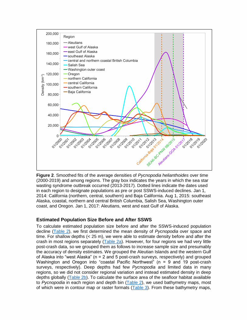
Figure 2. Smoothed fits of the average densities of Pycnopodia helianthoides over time (2000-2019) and among regions. The gray box indicates the years in which the sea star wasting syndrome outbreak occurred (2013-2017). Dotted lines indicate the dates used in each region to designate populations as pre or post SSWS-induced declines. Jan 1, 2014: California (northern, central, southern) and Baja California. Aug 1, 2015: southeast Alaska, coastal, northern and central British Columbia, Salish Sea, Washington outer coast, and Oregon. Jan 1, 2017: Aleutians, west and east Gulf of Alaska.
Estimated Population Size Before and After SSWS
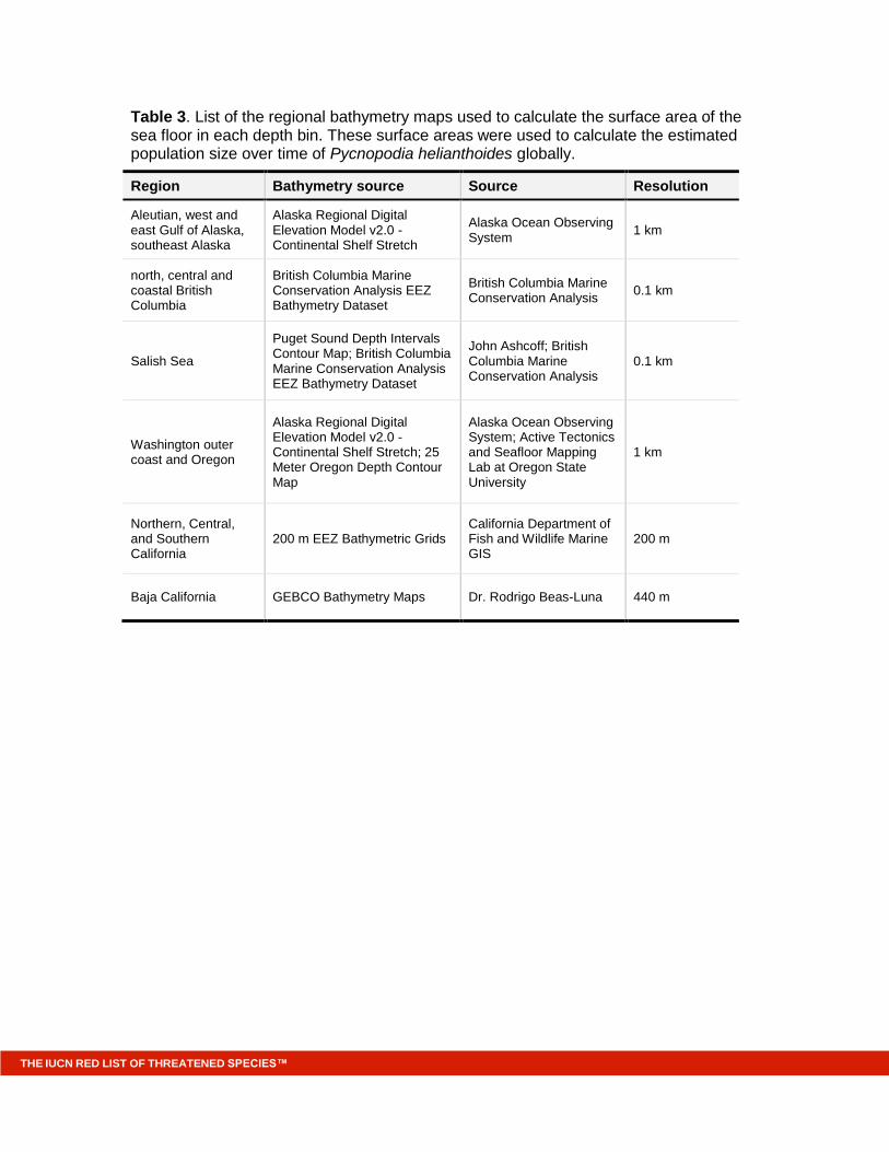
To calculate estimated population size before and after the SSWS-induced population decline (Table 2), we first determined the mean density of Pycnopodia over space and time. For shallow depths (< 25 m), we were able to estimate density before and after the crash in most regions separately (Table 2a). However, for four regions we had very little post-crash data, so we grouped them as follows to increase sample size and presumably the accuracy of density estimates. We grouped the Aleutian Islands and the western Gulf of Alaska into “west Alaska” (n = 2 and 5 post-crash surveys, respectively) and grouped Washington and Oregon into “coastal Pacific Northwest” (n = 9 and 19 post-crash surveys, respectively). Deep depths had few Pycnopodia and limited data in many regions, so we did not consider regional variation and instead estimated density in deep depths globally (Table 2b). To calculate the surface area of the seafloor habitat available to Pycnopodia in each region and depth bin (Table 2), we used bathymetry maps, most of which were in contour map or raster formats (Table 3). From these bathymetry maps,
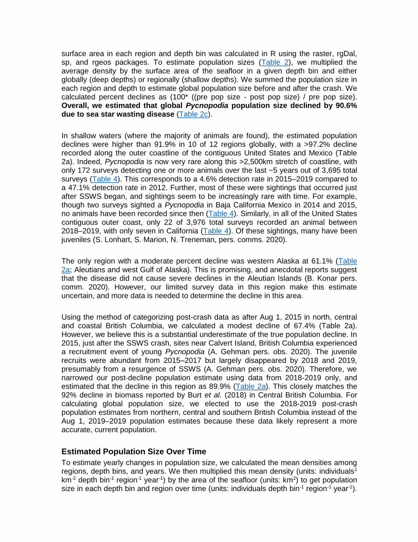
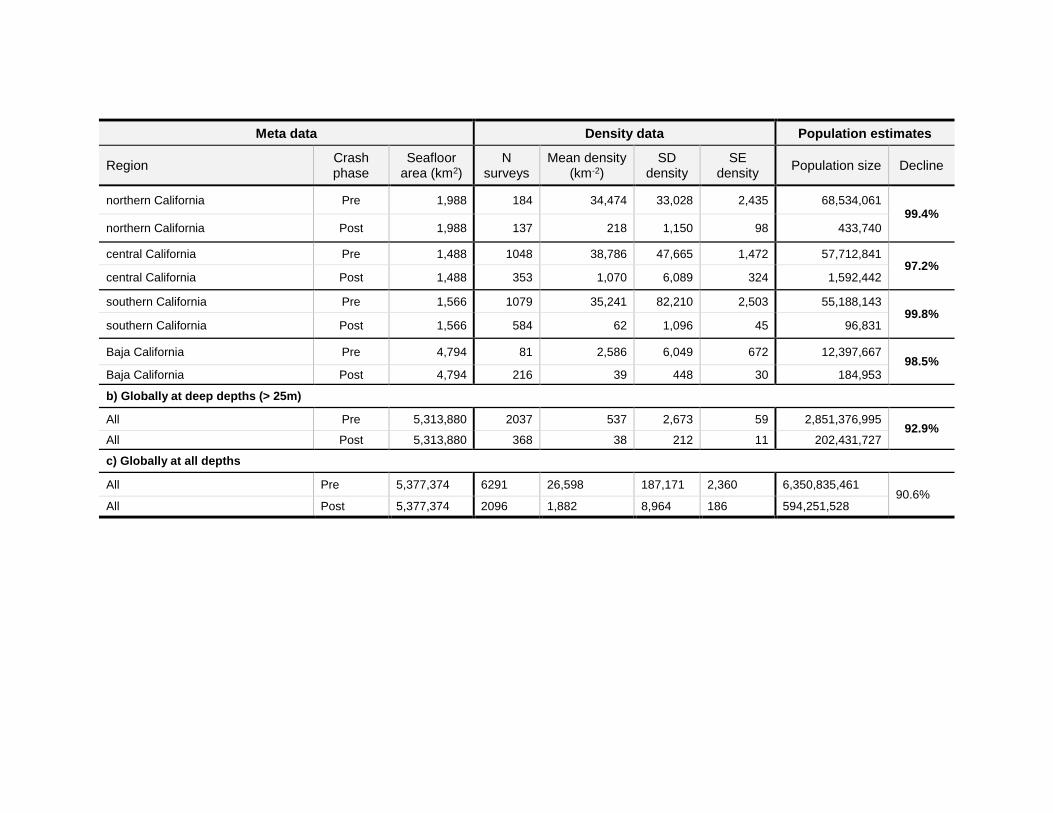
surface area in each region and depth bin was calculated in R using the raster, rgDal, sp, and rgeos packages. To estimate population sizes (Table 2), we multiplied the average density by the surface area of the seafloor in a given depth bin and either globally (deep depths) or regionally (shallow depths). We summed the population size in each region and depth to estimate global population size before and after the crash. We calculated percent declines as (100* ((pre pop size - post pop size) / pre pop size). Overall, we estimated that global Pycnopodia population size declined by 90.6% due to sea star wasting disease (Table 2c).
In shallow waters (where the majority of animals are found), the estimated population declines were higher than 91.9% in 10 of 12 regions globally, with a >97.2% decline recorded along the outer coastline of the contiguous United States and Mexico (Table 2a). Indeed, Pycnopodia is now very rare along this >2,500km stretch of coastline, with only 172 surveys detecting one or more animals over the last ~5 years out of 3,695 total surveys (Table 4). This corresponds to a 4.6% detection rate in 2015‒2019 compared to a 47.1% detection rate in 2012. Further, most of these were sightings that occurred just after SSWS began, and sightings seem to be increasingly rare with time. For example, though two surveys sighted a Pycnopodia in Baja California Mexico in 2014 and 2015, no animals have been recorded since then (Table 4). Similarly, in all of the United States contiguous outer coast, only 22 of 3,976 total surveys recorded an animal between 2018‒2019, with only seven in California (Table 4). Of these sightings, many have been juveniles (S. Lonhart, S. Marion, N. Treneman, pers. comms. 2020).
The only region with a moderate percent decline was western Alaska at 61.1% (Table 2a; Aleutians and west Gulf of Alaska). This is promising, and anecdotal reports suggest that the disease did not cause severe declines in the Aleutian Islands (B. Konar pers. comm. 2020). However, our limited survey data in this region make this estimate uncertain, and more data is needed to determine the decline in this area.
Using the method of categorizing post-crash data as after Aug 1, 2015 in north, central and coastal British Columbia, we calculated a modest decline of 67.4% (Table 2a). However, we believe this is a substantial underestimate of the true population decline. In 2015, just after the SSWS crash, sites near Calvert Island, British Columbia experienced a recruitment event of young Pycnopodia (A. Gehman pers. obs. 2020). The juvenile recruits were abundant from 2015‒2017 but largely disappeared by 2018 and 2019, presumably from a resurgence of SSWS (A. Gehman pers. obs. 2020). Therefore, we narrowed our post-decline population estimate using data from 2018-2019 only, and estimated that the decline in this region as 89.9% (Table 2a). This closely matches the 92% decline in biomass reported by Burt et al. (2018) in Central British Columbia. For calculating global population size, we elected to use the 2018-2019 post-crash population estimates from northern, central and southern British Columbia instead of the Aug 1, 2019‒2019 population estimates because these data likely represent a more accurate, current population.
Estimated Population Size Over Time
To estimate yearly changes in population size, we calculated the mean densities among regions, depth bins, and years. We then multiplied this mean density (units: individuals1 km-2 depth bin-1 region-1 year-1) by the area of the seafloor (units: km2) to get population size in each depth bin and region over time (units: individuals depth bin-1 region-1 year-1).
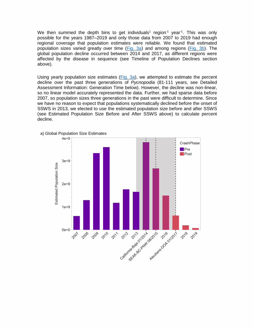
We then summed the depth bins to get individuals1 region-1 year-1. This was only possible for the years 1987‒2019 and only those data from 2007 to 2019 had enough regional coverage that population estimates were reliable. We found that estimated population sizes varied greatly over time (Fig. 3a) and among regions (Fig. 3b). The global population decline occurred between 2014 and 2017, as different regions were affected by the disease in sequence (see Timeline of Population Declines section above).
Using yearly population size estimates (Fig. 3a), we attempted to estimate the percent decline over the past three generations of Pycnopodia (81-111 years, see Detailed Assessment Information: Generation Time below). However, the decline was non-linear, so no linear model accurately represented the data. Further, we had sparse data before 2007, so population sizes three generations in the past were difficult to determine. Since we have no reason to expect that populations systematically declined before the onset of SSWS in 2013, we elected to use the estimated population size before and after SSWS (see Estimated Population Size Before and After SSWS above) to calculate percent decline.
a) Global Population Size Estimates
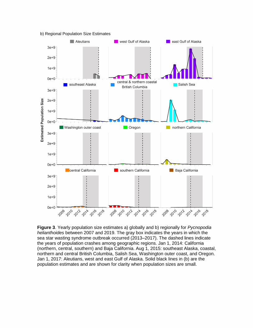
Figure 3. Yearly population size estimates a) globally and b) regionally for Pycnopodia helianthoides between 2007 and 2019. The gray box indicates the years in which the sea star wasting syndrome outbreak occurred (2013‒2017). The dashed lines indicate the years of population crashes among geographic regions. Jan 1, 2014: California (northern, central, southern) and Baja California. Aug 1, 2015: southeast Alaska, coastal, northern and central British Columbia, Salish Sea, Washington outer coast, and Oregon. Jan 1, 2017: Aleutians, west and east Gulf of Alaska. Solid black lines in (b) are the population estimates and are shown for clarity when population sizes are small.
b) Regional Population Size Estimates
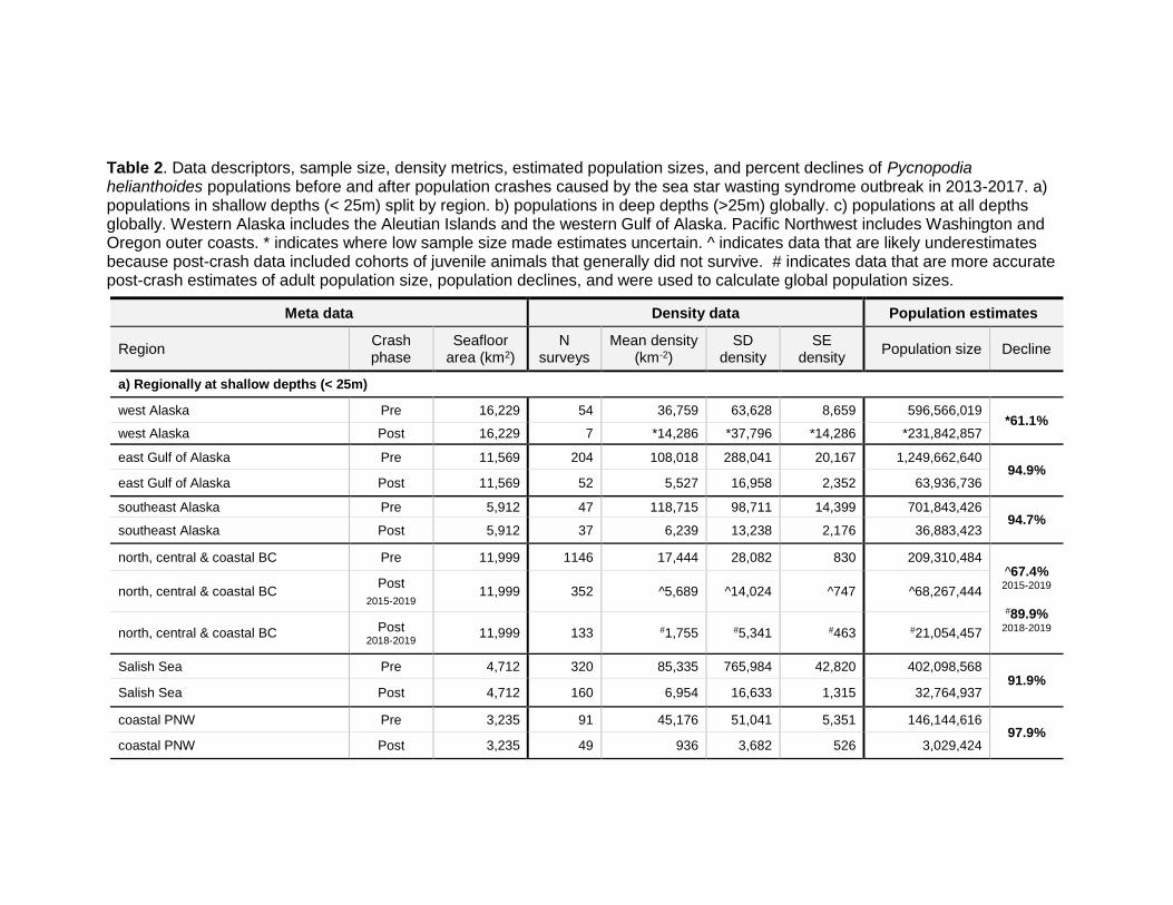
Table 2. Data descriptors, sample size, density metrics, estimated population sizes, and percent declines of Pycnopodia helianthoides populations before and after population crashes caused by the sea star wasting syndrome outbreak in 2013-2017. a) populations in shallow depths (< 25m) split by region. b) populations in deep depths (>25m) globally. c) populations at all depths globally. Western Alaska includes the Aleutian Islands and the western Gulf of Alaska. Pacific Northwest includes Washington and Oregon outer coasts. * indicates where low sample size made estimates uncertain. ^ indicates data that are likely underestimates because post-crash data included cohorts of juvenile animals that generally did not survive. # indicates data that are more accurate post-crash estimates of adult population size, population declines, and were used to calculate global population sizes.
Meta data Density data Population estimates
Region Crash phase
Seafloor area (km2)
N surveys
Mean density (km-2)
SD density
SE density
Population size Decline
a) Regionally at shallow depths (< 25m)
west Alaska Pre 16,229 54 36,759 63,628 8,659 596,566,019 *61.1%
west Alaska Post 16,229 7 *14,286 *37,796 *14,286 *231,842,857
east Gulf of Alaska Pre 11,569 204 108,018 288,041 20,167 1,249,662,640 94.9%
east Gulf of Alaska Post 11,569 52 5,527 16,958 2,352 63,936,736
southeast Alaska Pre 5,912 47 118,715 98,711 14,399 701,843,426 94.7%
southeast Alaska Post 5,912 37 6,239 13,238 2,176 36,883,423
north, central & coastal BC Pre 11,999 1146 17,444 28,082 830 209,310,484 ^67.4% 2015-2019
#89.9%
2018-2019
north, central & coastal BC Post
2015-2019 11,999 352 ^5,689 ^14,024 ^747 ^68,267,444
north, central & coastal BC Post 2018-2019
11,999 133 #1,755 #5,341 #463 #21,054,457
Salish Sea Pre 4,712 320 85,335 765,984 42,820 402,098,568 91.9%
Salish Sea Post 4,712 160 6,954 16,633 1,315 32,764,937
coastal PNW Pre 3,235 91 45,176 51,041 5,351 146,144,616 97.9%
coastal PNW Post 3,235 49 936 3,682 526 3,029,424
Meta data Density data Population estimates
Region Crash phase
Seafloor area (km2)
N surveys
Mean density (km-2)
SD density
SE density
Population size Decline
northern California Pre 1,988 184 34,474 33,028 2,435 68,534,061 99.4%
northern California Post 1,988 137 218 1,150 98 433,740
central California Pre 1,488 1048 38,786 47,665 1,472 57,712,841 97.2%
central California Post 1,488 353 1,070 6,089 324 1,592,442
southern California Pre 1,566 1079 35,241 82,210 2,503 55,188,143 99.8%
southern California Post 1,566 584 62 1,096 45 96,831
Baja California Pre 4,794 81 2,586 6,049 672 12,397,667 98.5%
Baja California Post 4,794 216 39 448 30 184,953
b) Globally at deep depths (> 25m)
All Pre 5,313,880 2037 537 2,673 59 2,851,376,995 92.9%
All Post 5,313,880 368 38 212 11 202,431,727
c) Globally at all depths
All Pre 5,377,374 6291 26,598 187,171 2,360 6,350,835,461 90.6%
All Post 5,377,374 2096 1,882 8,964 186 594,251,528
THE IUCN RED LIST OF THREATENED SPECIES™
Table 3. List of the regional bathymetry maps used to calculate the surface area of the sea floor in each depth bin. These surface areas were used to calculate the estimated population size over time of Pycnopodia helianthoides globally.
Region Bathymetry source Source Resolution
Aleutian, west and east Gulf of Alaska, southeast Alaska
Alaska Regional Digital Elevation Model v2.0 - Continental Shelf Stretch
Alaska Ocean Observing System
1 km
north, central and coastal British Columbia
British Columbia Marine Conservation Analysis EEZ Bathymetry Dataset
British Columbia Marine Conservation Analysis
0.1 km
Salish Sea
Puget Sound Depth Intervals Contour Map; British Columbia Marine Conservation Analysis EEZ Bathymetry Dataset
John Ashcoff; British Columbia Marine Conservation Analysis
0.1 km
Washington outer coast and Oregon
Alaska Regional Digital Elevation Model v2.0 - Continental Shelf Stretch; 25 Meter Oregon Depth Contour Map
Alaska Ocean Observing System; Active Tectonics and Seafloor Mapping Lab at Oregon State University
1 km
Northern, Central, and Southern California
200 m EEZ Bathymetric Grids California Department of Fish and Wildlife Marine GIS
200 m
Baja California GEBCO Bathymetry Maps Dr. Rodrigo Beas-Luna 440 m
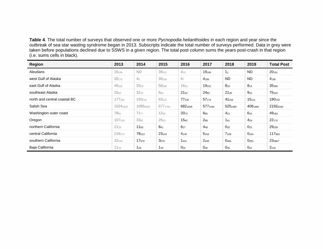
Table 4. The total number of surveys that observed one or more Pycnopodia helianthoides in each region and year since the outbreak of sea star wasting syndrome began in 2013. Subscripts indicate the total number of surveys performed. Data in grey were taken before populations declined due to SSWS in a given region. The total post column sums the years post-crash in that region (i.e. sums cells in black).
Region 2013 2014 2015 2016 2017 2018 2019 Total Post
Aleutians 16156 ND 39221 410 19150 11 ND 20151
west Gulf of Alaska 20172 45 30238 67 4156 ND ND 4156
east Gulf of Alaska 45202 2629 58285 1633 19231 815 814 35260
southeast Alaska 2564 3242 684 2122 2482 2135 915 75154
north and central coastal BC 177265 150214 63212 77235 57172 41225 15121 190753
Salish Sea 16241932 10852032 6771764 6821659 5771542 5251482 4081483 21926166
Washington outer coast 7881 7177 1290 3373 685 415 610 49183
Oregon 107159 3387 2553 1542 268 141 424 22175
northern California 2125 1150 841 627 448 033 010 29209
central California 216274 78213 23144 4140 5153 7109 0104 117863
southern California 32446 17670 3575 1421 2448 0400 0353 232867
Baja California 1135 128 129 032 040 045 042 2216
THE IUCN RED LIST OF THREATENED SPECIES™
Densities Among Regions and Depths
Methods. We used models to detect patterns in population density before and after SSWS among the regions and depths. Due to sparse data coverage in the deep depths but ample coverage in shallow depths (Fig. 4), we elected to perform separate models for these two depth bins. Similar to our analyses for population size, data for deep depths were unavailable for many regions (Fig. 4) so we did not consider regional variation in the model. For shallow depths (< 25m), we had enough data to analyze population densities of most of the regions separately, but we grouped the Aleutian Islands and the western Gulf of Alaska into “west Alaska” and coastal Washington and Oregon into “coastal Pacific Northwest” to increase our accuracy in estimating post-crash density. We performed models in JMP Pro 14 (SAS) using generalized linear models (GLMs) with Pycnopodia count as the response variable, log(area) as the offset variable, Poisson distributions, and log link functions. Crash phase (pre/post) was a response in both models. For the shallow model we also included region (grouped as above) and its interaction with the crash phase.
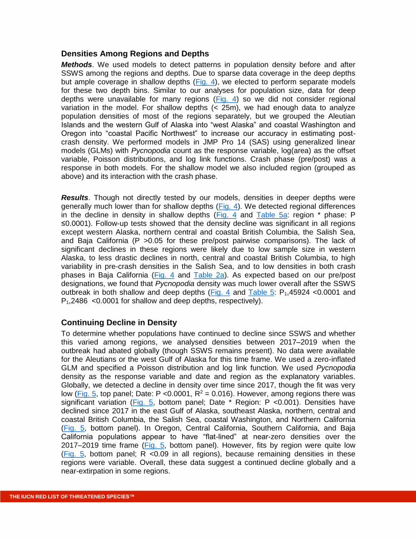
Results. Though not directly tested by our models, densities in deeper depths were generally much lower than for shallow depths (Fig. 4). We detected regional differences in the decline in density in shallow depths (Fig. 4 and Table 5a: region * phase: P ≤0.0001). Follow-up tests showed that the density decline was significant in all regions except western Alaska, northern central and coastal British Columbia, the Salish Sea, and Baja California (P >0.05 for these pre/post pairwise comparisons). The lack of significant declines in these regions were likely due to low sample size in western Alaska, to less drastic declines in north, central and coastal British Columbia, to high variability in pre-crash densities in the Salish Sea, and to low densities in both crash phases in Baja California (Fig. 4 and Table 2a). As expected based on our pre/post designations, we found that Pycnopodia density was much lower overall after the SSWS outbreak in both shallow and deep depths (Fig. 4 and Table 5: P1,45924 <0.0001 and P1,2486 <0.0001 for shallow and deep depths, respectively).
Continuing Decline in Density
To determine whether populations have continued to decline since SSWS and whether this varied among regions, we analysed densities between 2017‒2019 when the outbreak had abated globally (though SSWS remains present). No data were available for the Aleutians or the west Gulf of Alaska for this time frame. We used a zero-inflated GLM and specified a Poisson distribution and log link function. We used Pycnopodia density as the response variable and date and region as the explanatory variables. Globally, we detected a decline in density over time since 2017, though the fit was very low (Fig. 5, top panel; Date: P <0.0001, R2 = 0.016). However, among regions there was significant variation (Fig. 5, bottom panel; Date * Region: P <0.001). Densities have declined since 2017 in the east Gulf of Alaska, southeast Alaska, northern, central and coastal British Columbia, the Salish Sea, coastal Washington, and Northern California (Fig. 5, bottom panel). In Oregon, Central California, Southern California, and Baja California populations appear to have “flat-lined” at near-zero densities over the 2017‒2019 time frame (Fig. 5, bottom panel). However, fits by region were quite low (Fig. 5, bottom panel; R <0.09 in all regions), because remaining densities in these regions were variable. Overall, these data suggest a continued decline globally and a near-extirpation in some regions.
Table 5. Generalised linear model results analyzing the trends in Pycnopodia helianthoides densities among a) crash phases and regions at shallow depths (<25 m) and b) crash phases in all regions at deep depths (>25 m).
Term df Chi Sq. P
a) Shallow Density Model
Crash Phase 1 22.03 <0.0001
Region 9 34.79 <0.0001
Crash Phase * Region 9 34.50 <0.0001
b) Deep Density Model
Crash Phase 1 26.27 <0.0001
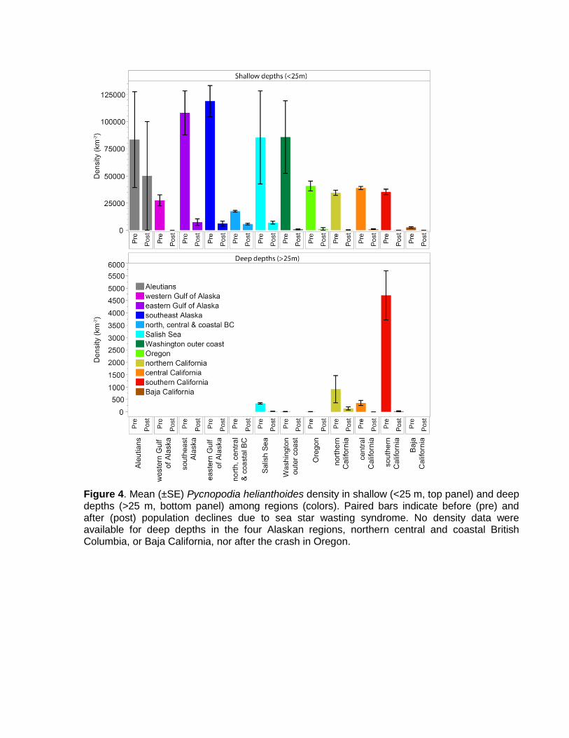
Figure 4. Mean (±SE) Pycnopodia helianthoides density in shallow (<25 m, top panel) and deep depths (>25 m, bottom panel) among regions (colors). Paired bars indicate before (pre) and after (post) population declines due to sea star wasting syndrome. No density data were available for deep depths in the four Alaskan regions, northern central and coastal British Columbia, or Baja California, nor after the crash in Oregon.
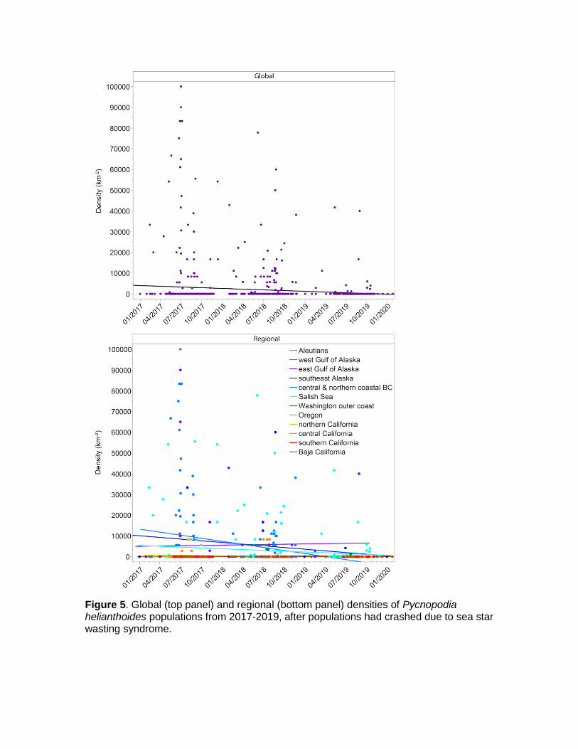
Figure 5. Global (top panel) and regional (bottom panel) densities of Pycnopodia helianthoides populations from 2017-2019, after populations had crashed due to sea star wasting syndrome.
Habitats and Ecology
Diet
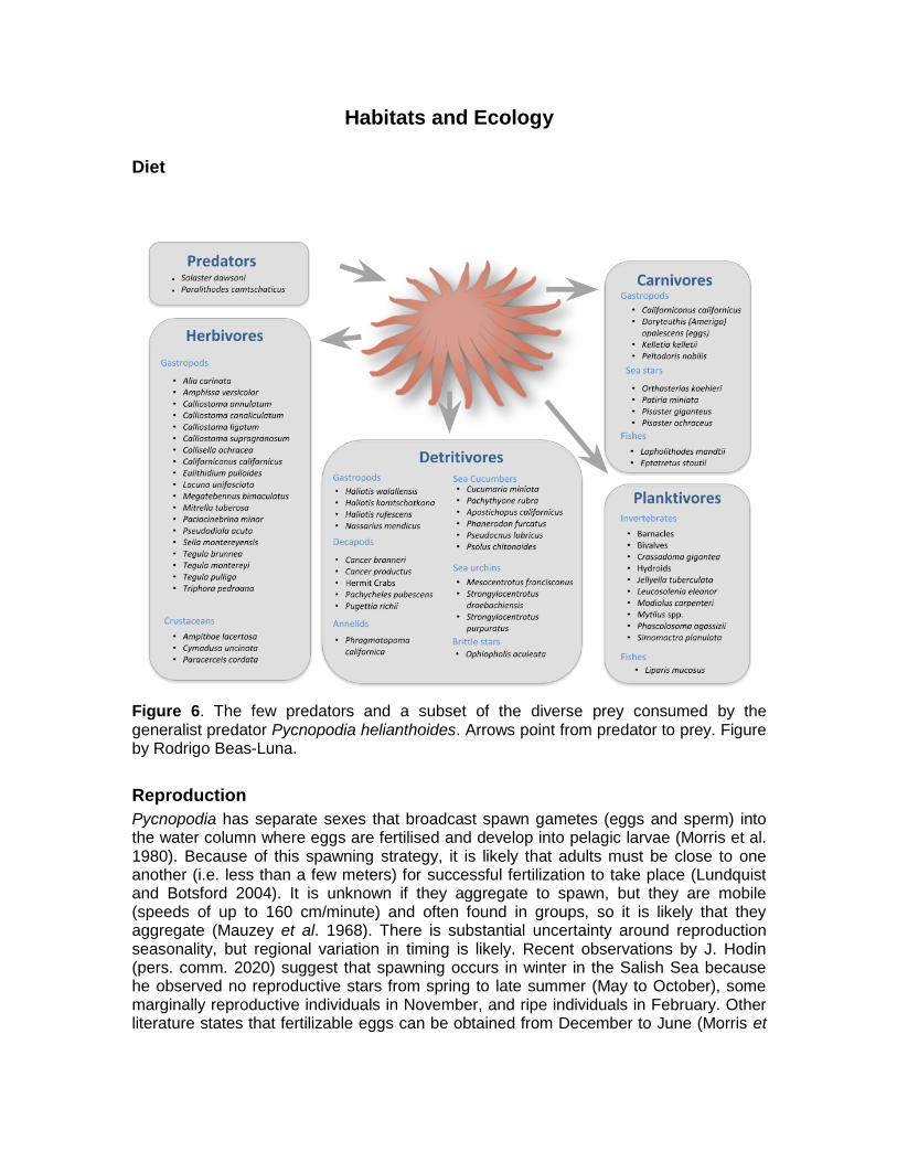
Figure 6. The few predators and a subset of the diverse prey consumed by the generalist predator Pycnopodia helianthoides. Arrows point from predator to prey. Figure by Rodrigo Beas-Luna.
Reproduction
Pycnopodia has separate sexes that broadcast spawn gametes (eggs and sperm) into the water column where eggs are fertilised and develop into pelagic larvae (Morris et al. 1980). Because of this spawning strategy, it is likely that adults must be close to one another (i.e. less than a few meters) for successful fertilization to take place (Lundquist and Botsford 2004). It is unknown if they aggregate to spawn, but they are mobile (speeds of up to 160 cm/minute) and often found in groups, so it is likely that they aggregate (Mauzey et al. 1968). There is substantial uncertainty around reproduction seasonality, but regional variation in timing is likely. Recent observations by J. Hodin (pers. comm. 2020) suggest that spawning occurs in winter in the Salish Sea because he observed no reproductive stars from spring to late summer (May to October), some marginally reproductive individuals in November, and ripe individuals in February. Other literature states that fertilizable eggs can be obtained from December to June (Morris et
al. 1980) or that the breeding season is May through June surrounding Vancouver, Island, British Columbia (Feder and Christensen 1966).
After fertilization, the embryos quickly develop into swimming, bilateral larvae that progress through the typical echinoderm larval phases of prism, bipinnaria, and pluteus larvae (Morris et al. 1980). The larvae feed on single-celled phytoplankton (Greer 1962). The length of the larval period is at least 50 days (J. Hodin pers. comm. 2020) but up to 146 days (Strathmann 1978). Most larvae metamorphose after 60-70 days into a juvenile sea star with five arms, and they grow more arms over time (Greer 1962).
While no studies have been conducted specifically on the age of maturity of Pycnopodia, we estimate it to be at least 5 years based on the age of first reproduction for Pisaster ochraceus (Menge 1975), a well-studied predatory sea star that lives in similar habitats, has some overlap in diet, and has a similar reproductive strategy (Giese et al. 1991, Menge 1975, Sewell and Watson 1993). It also is quite likely that Pycnopodia, like Pisaster ochraceus, increases in fecundity as it increases in size (S. Gravem and B. Menge, unpublished data).
Life History and Longevity
Sea stars are known to have indeterminate growth, meaning that individual growth rates and maximum size are strongly dependent on environmental factors like water temperature and food availability (Gooding et al. 2009, Sebens 1987). Because of this, it is difficult to age sea stars in the wild because their size does not provide a reliable indication of age. Usually, laboratory studies or cohort analyses are needed to understand sea star growth rates. However, Pycnopodia is notoriously difficult to maintain in captivity, resulting in limited controlled studies of its growth. Subsequently, although this species is frequently recorded on dive surveys, very limited data are available on growth, survival, and reproduction of Pycnopodia in captivity and in the wild. We were unable to find scientific literature that documented Pycnopodia growth rates, likely because they are extremely hard to tag individually. However, we did identify:
- Anecdotal evidence that juvenile Pycnopodia grow at a rate of roughly 5cm/year in diameter during the first several years of life in captivity (C. Long. pers. comm. 2020)
- A post-outbreak analysis of growth in juvenile wild Pycnopodia in central British Columbia that estimated early growth rates of 3-8 cm/year in diameter (A. Gehman. pers. obs. 2020)
- Anecdotal evidence that 30 captive mid-sized Pycnopodia (sizes 30‒60 cm) at Friday Harbor Labs in Washington grew at a median rate of roughly 2 cm/year (J. Hodin, pers. comm. 2020).
- A report of a Pycnopodia at the Rotterdam Zoo, Netherlands that grew from 30 cm to 60 cm in 15 years, a rate about 2 cm/year
Unfortunately, the literature on sea star growth curves is sparse. What evidence does exist suggests that sea stars with adequate food grow exponentially within their first year (Lucas 1984, Wilmes et al. 2017, Yamaguchi 1974). However, after the first year growth rates begin to slow and eventually asymptote (Bos et al. 2008, Keesing 2017). That sea
stars have growth rates that decline over their lifetime is corroborated by literature on sea urchins, who are fellow echinoderms. There is a substantial body of literature that examines how the growth rates for sea urchins decrease over their lifetime with various experts preferring to model their growth curves using Von Bertalanffy, Richards, Tanaka, and logistic-dose models (Ebert and Russell 1992, Rogers-Bennett et al. 2003). Since the sea star literature also regularly uses the Von Bertalanffy model to estimate growth curves (Bos et al. 2008, Keesing 2017), we used this growth equation to estimate Pycnopodia life span.
Von Bertalanffy growth equation:
L=L∞ (1-e(-Ka))
with L = diameter in centimeters at age a, L∞ = maximum length in centimeters, K = the
Von Bertalanffy growth parameter in cm yr-1, and a = age in years. We set L∞ = 100 cm
as Pycnopodia is rarely found larger than this (Mauzey et al. 1968).
Alternatively, we can also use a Richards growth curve to represent theoretical Pycnopodia growth over lifetime. The Richards model is commonly used to describe sea urchin growth curves. It also allows for higher initial growth and slower growth later in life than the Von Bertalanffy model, a feature that several sea star experts suggested may be more realistic for Pycnopodia.
Richard’s growth equation:
L= L∞ (1-b*e(-Ka))-n
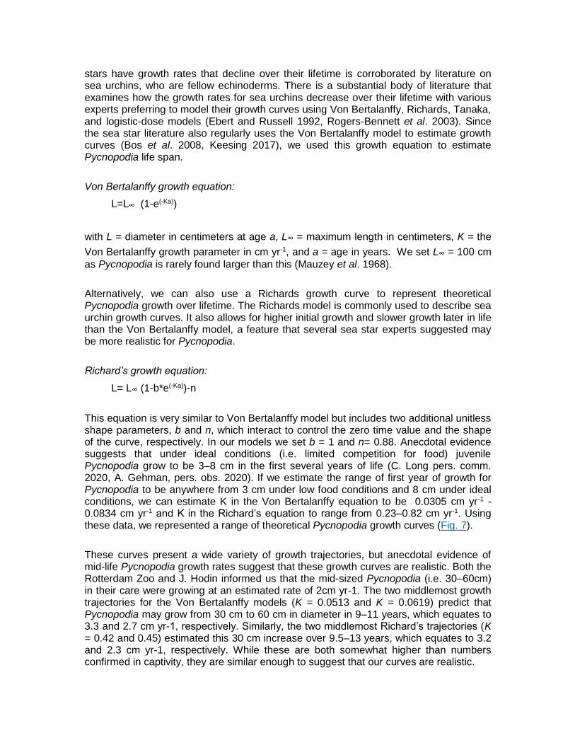
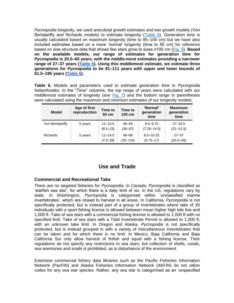
This equation is very similar to Von Bertalanffy model but includes two additional unitless shape parameters, b and n, which interact to control the zero time value and the shape of the curve, respectively. In our models we set b = 1 and n= 0.88. Anecdotal evidence suggests that under ideal conditions (i.e. limited competition for food) juvenile Pycnopodia grow to be 3‒8 cm in the first several years of life (C. Long pers. comm. 2020, A. Gehman, pers. obs. 2020). If we estimate the range of first year of growth for Pycnopodia to be anywhere from 3 cm under low food conditions and 8 cm under ideal conditions, we can estimate K in the Von Bertalanffy equation to be 0.0305 cm yr-1 - 0.0834 cm yr-1 and K in the Richard’s equation to range from 0.23‒0.82 cm yr-1. Using these data, we represented a range of theoretical Pycnopodia growth curves (Fig. 7).
These curves present a wide variety of growth trajectories, but anecdotal evidence of mid-life Pycnopodia growth rates suggest that these growth curves are realistic. Both the Rotterdam Zoo and J. Hodin informed us that the mid-sized Pycnopodia (i.e. 30‒60cm) in their care were growing at an estimated rate of 2cm yr-1. The two middlemost growth trajectories for the Von Bertalanffy models (K = 0.0513 and K = 0.0619) predict that Pycnopodia may grow from 30 cm to 60 cm in diameter in 9‒11 years, which equates to 3.3 and 2.7 cm yr-1, respectively. Similarly, the two middlemost Richard’s trajectories (K = 0.42 and 0.45) estimated this 30 cm increase over 9.5‒13 years, which equates to 3.2 and 2.3 cm yr-1, respectively. While these are both somewhat higher than numbers confirmed in captivity, they are similar enough to suggest that our curves are realistic.
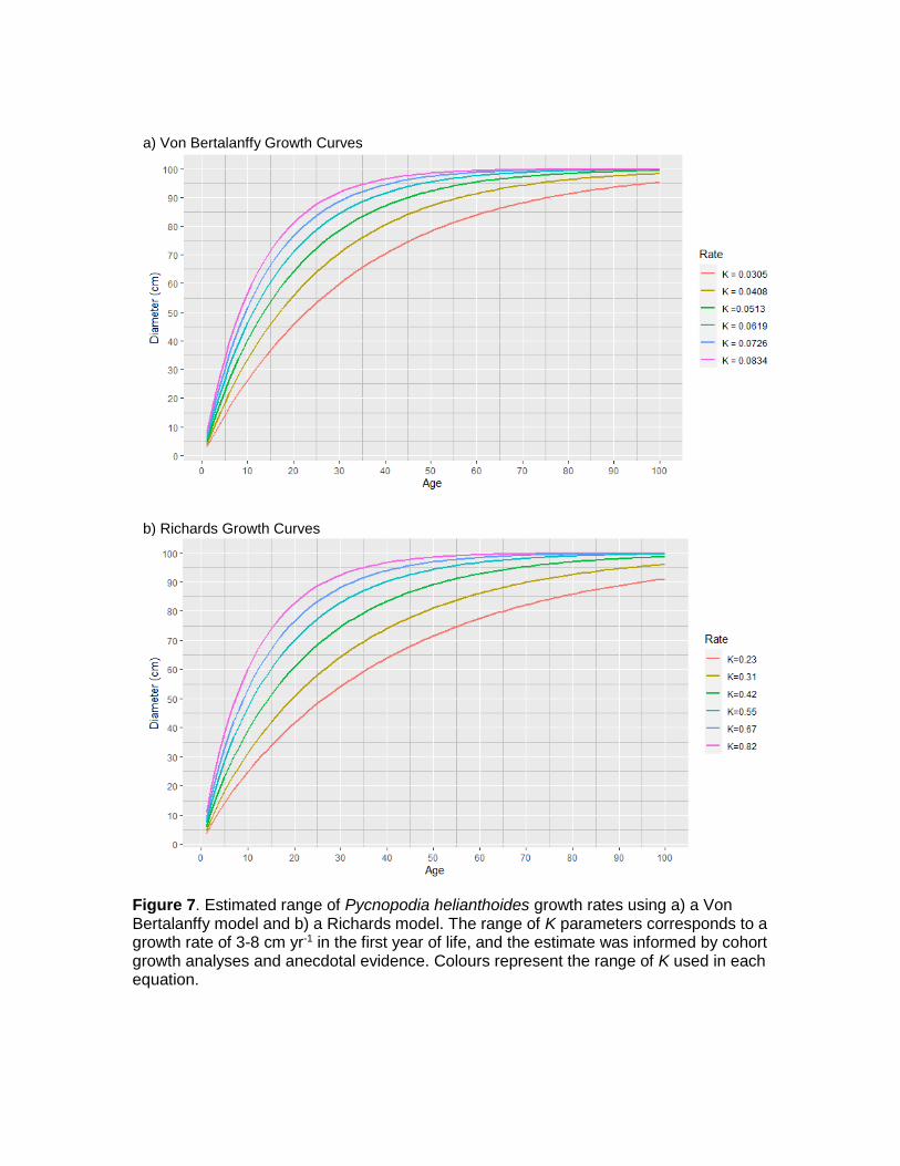
Figure 7. Estimated range of Pycnopodia helianthoides growth rates using a) a Von Bertalanffy model and b) a Richards model. The range of K parameters corresponds to a growth rate of 3-8 cm yr-1 in the first year of life, and the estimate was informed by cohort growth analyses and anecdotal evidence. Colours represent the range of K used in each equation.
b) Richards Growth Curves
a) Von Bertalanffy Growth Curves
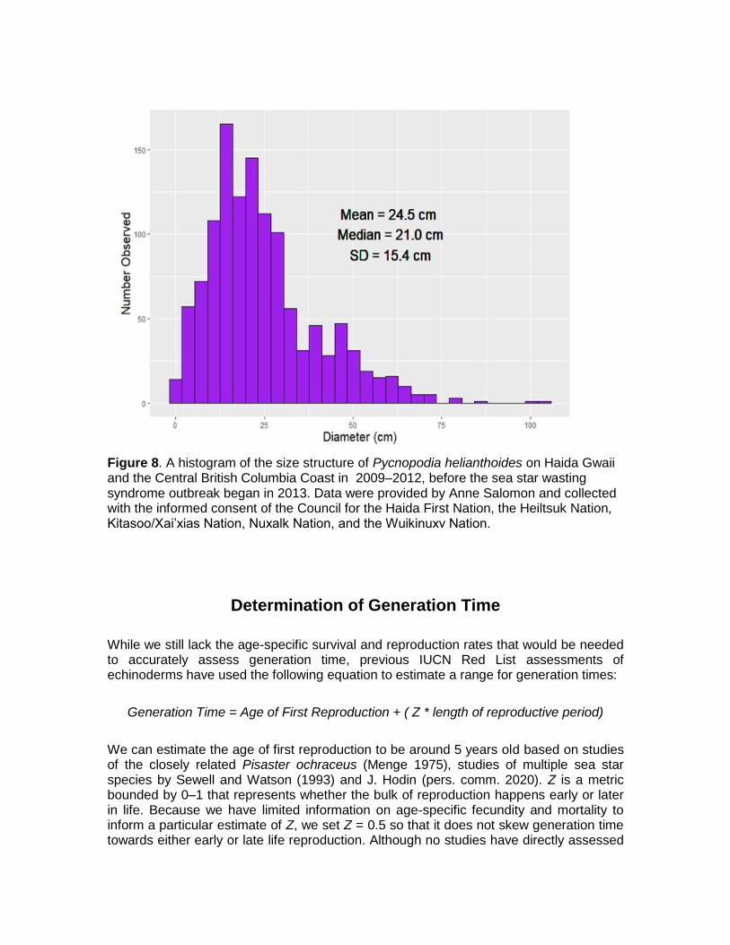
Figure 8. A histogram of the size structure of Pycnopodia helianthoides on Haida Gwaii and the Central British Columbia Coast in 2009‒2012, before the sea star wasting syndrome outbreak began in 2013. Data were provided by Anne Salomon and collected with the informed consent of the Council for the Haida First Nation, the Heiltsuk Nation, Kitasoo/Xai’xias Nation, Nuxalk Nation, and the Wuikinuxv Nation.
Determination of Generation Time
While we still lack the age-specific survival and reproduction rates that would be needed to accurately assess generation time, previous IUCN Red List assessments of echinoderms have used the following equation to estimate a range for generation times:
Generation Time = Age of First Reproduction + ( Z * length of reproductive period)
We can estimate the age of first reproduction to be around 5 years old based on studies of the closely related Pisaster ochraceus (Menge 1975), studies of multiple sea star species by Sewell and Watson (1993) and J. Hodin (pers. comm. 2020). Z is a metric bounded by 0‒1 that represents whether the bulk of reproduction happens early or later in life. Because we have limited information on age-specific fecundity and mortality to inform a particular estimate of Z, we set Z = 0.5 so that it does not skew generation time towards either early or late life reproduction. Although no studies have directly assessed
Pycnopodia longevity, we used anecdotal growth estimates and two growth models (Von Bertalanffy and Richards models) to estimate longevity (Table 6). Generation time is usually calculated based on maximum longevity (time to 95‒100 cm) but we have also included estimates based on a more ‘normal’ longevity (time to 50 cm) for reference based on size structure data that shows few stars grow to sizes ≥100 cm (Fig. 8). Based on the available models, our range of estimates for generation time for Pycnopodia is 20.5‒65 years, with the middle-most estimates providing a narrower range of 27‒37 years (Table 6). Using this middlemost estimate, we estimate three generations for Pycnopodia to be 81‒111 years with upper and lower bounds of 61.5‒195 years (Table 6).
Table 6. Models and parameters used to estimate generation time in Pycnopodia helianthoides. In the “Time” columns, the top range of years were calculated with our middlemost estimates of longevity (see Fig. 7) and the bottom range in parentheses were calculated using the maximum and minimum estimates of our longevity models.
Model Age of first
reproduction Time to 50 cm
Time to 100 cm
‘Normal’ generation
time
Maximum generation
time
Von Bertalanffy 5 years 11‒13.5
(8.5‒23)
48‒59
(36‒97)
8.5‒9.75
(7.25‒14.5)
27–32.5
(21–51.5)
Richards 5 years 11‒14.5
(7.5‒28)
48‒68
(35‒124)
8.5–10.25
(6.75–17)
27–37
(20.5–65)
Use and Trade
Commercial and Recreational Take
There are no targeted fisheries for Pycnopodia. In Canada, Pycnopodia is classified as ‘starfish sea star’, for which there is a daily limit of six. In the US, regulations vary by state. In Washington, Pycnopodia is categorised within ‘unclassified marine invertebrates’, which are closed to harvest in all areas. In California, Pycnopodia is not specifically protected, but is instead part of a group of invertebrates where take of 35 individuals with a sport fishing license is allowed between mean higher high tide line and 1,000 ft. Take of sea stars with a commercial fishing license is allowed to 1,000 ft with no specified limit. Take of sea stars with a Tidal Invertebrate Permit is allowed to 1,000 ft, with an unknown take limit. In Oregon and Alaska, Pycnopodia is not specifically protected, but is instead grouped in with a variety of miscellaneous invertebrates that can be taken and for which there is no limit. In Mexico, Baja California and Baja California Sur only allow harvest of finfish and squid with a fishing license. Their regulations do not specify any restrictions to sea stars, but collection of shells, corals, sea anemones and snails is prohibited, as is disturbance of the environment.
Extensive commercial fishery data libraries such as the Pacific Fisheries Information Network (PacFIN) and Alaska Fisheries Information Network (AKFIN) do not utilize codes for any sea star species. Rather, any sea star is categorised as an ‘unspecified
echinoderm’. Although most regions along the Pacific Coast technically permit some allowable personal-use and commercial harvest of Pycnopodia, all indications suggest that the harvest rate is extremely low, relatively undetectable, and perhaps absent.
Scientific Collection
Scientific collection permits in Alaska, Canada, Washington, Oregon, and California all require an application process that is reviewed by a panel of biologists, in their respective regions, to approve/deny lethal or non-lethal take of each species listed. Since the SSWS outbreak, applications in Washington, Oregon, and California have restricted or limited any lethal take of Pycnopodia to only research applications directly related to the assessment or recovery of Pycnopodia. At this time, Alaska does not restrict take of Pycnopodia for scientific collection. We lack information on the scientific take process in Mexico.
Bycatch
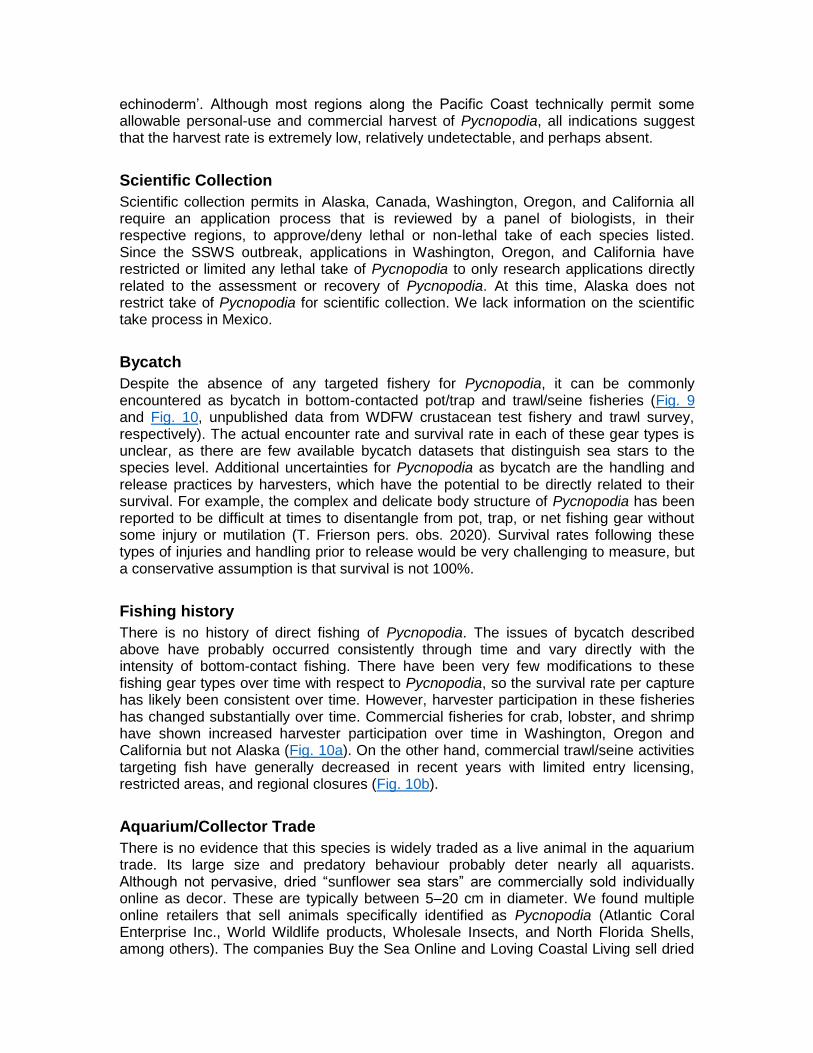
Despite the absence of any targeted fishery for Pycnopodia, it can be commonly encountered as bycatch in bottom-contacted pot/trap and trawl/seine fisheries (Fig. 9 and Fig. 10, unpublished data from WDFW crustacean test fishery and trawl survey, respectively). The actual encounter rate and survival rate in each of these gear types is unclear, as there are few available bycatch datasets that distinguish sea stars to the species level. Additional uncertainties for Pycnopodia as bycatch are the handling and release practices by harvesters, which have the potential to be directly related to their survival. For example, the complex and delicate body structure of Pycnopodia has been reported to be difficult at times to disentangle from pot, trap, or net fishing gear without some injury or mutilation (T. Frierson pers. obs. 2020). Survival rates following these types of injuries and handling prior to release would be very challenging to measure, but a conservative assumption is that survival is not 100%.
Fishing history
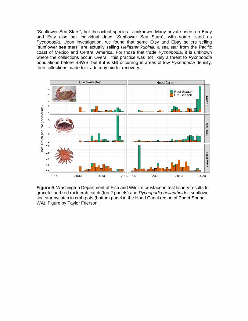
There is no history of direct fishing of Pycnopodia. The issues of bycatch described above have probably occurred consistently through time and vary directly with the intensity of bottom-contact fishing. There have been very few modifications to these fishing gear types over time with respect to Pycnopodia, so the survival rate per capture has likely been consistent over time. However, harvester participation in these fisheries has changed substantially over time. Commercial fisheries for crab, lobster, and shrimp have shown increased harvester participation over time in Washington, Oregon and California but not Alaska (Fig. 10a). On the other hand, commercial trawl/seine activities targeting fish have generally decreased in recent years with limited entry licensing, restricted areas, and regional closures (Fig. 10b).
Aquarium/Collector Trade
There is no evidence that this species is widely traded as a live animal in the aquarium trade. Its large size and predatory behaviour probably deter nearly all aquarists. Although not pervasive, dried “sunflower sea stars” are commercially sold individually online as decor. These are typically between 5‒20 cm in diameter. We found multiple online retailers that sell animals specifically identified as Pycnopodia (Atlantic Coral Enterprise Inc., World Wildlife products, Wholesale Insects, and North Florida Shells, among others). The companies Buy the Sea Online and Loving Coastal Living sell dried
“Sunflower Sea Stars”, but the actual species is unknown. Many private users on Ebay and Esty also sell individual dried “Sunflower Sea Stars”, with some listed as Pycnopodia. Upon investigation, we found that some Etsy and Ebay sellers selling “sunflower sea stars” are actually selling Heliaster kubiniji, a sea star from the Pacific coast of Mexico and Central America. For those that trade Pycnopodia, it is unknown where the collections occur. Overall, this practice was not likely a threat to Pycnopodia populations before SSWS, but if it is still occurring in areas of low Pycnopodia density, then collections made for trade may hinder recovery.
Figure 9. Washington Department of Fish and Wildlife crustacean test fishery results for graceful and red rock crab catch (top 2 panels) and Pycnopodia helianthoides sunflower sea star bycatch in crab pots (bottom panel in the Hood Canal region of Puget Sound, WA). Figure by Taylor Frierson.
Figure 10. Landings for a) commercial trap (crabs and lobsters) and commercial trawl (shrimp) fisheries and b) commercial trawl and seine fisheries in California (CA), Oregon (OR), Washington (WA) and Alaska (AK) since the 1960s. Figure by Vienna Saccomanno.
b) Commercial Landings of Fishes
a) Commercial Landings of Crustaceans
Threats
Disease
The SSWS epizootic affected over 20 species of sea stars (Hewson et al. 2014). First observed on the outer coast of Washington in June 2013, the epizootic was observed along the entire North American Pacific Coastline from Mexico to the Aleutian Islands by 2016 (see Miner et al. 2018 for details on the progression). Pycnopodia appears to be the species most negatively affected by the disease (Montecino-Latorre et al. 2016, Schultz et al. 2016, Harvell et al. 2019). While the pathogenesis of SSWS in Pycnopodia has not been well characterized, disease progresses from subtle dermal lesions often characterized by discoloration, then increasing lesion diameter and depth, followed by loss of turgor pressure and body wall ruptures, limb autotomisation and ultimately death, leaving behind piles of calcified ossicles (Schultz et al. 2016). Microscopically, lesions seen include epidermal necrosis and ulceration, and dermal inflammation and edema in the body wall (Hewson et al. 2014). Experimentally, inoculated Pycnopodia showed symptoms 8‒17 days post-exposure (Hewson et al. 2014) and field observations suggested that local populations could be extirpated within 21 days (Montecino-Latorre et al. 2016).
Signs of wasting in the 2013 outbreak were likely caused by disease agents, as aquariums that utilize UV sterilised sea water inflow did not see signs of disease, while disease did spread in non-treated aquariums (Hewson et al. 2014). However, the etiology or underlying cause for most asteroid wasting epizootics have been difficult to discern (Hewson et al. 2019) and there is still debate among scientists about the causative agent for the 2013 event (Hewson et al. 2018). Currently, wasting asteroid associated densoviruses (WAaDs, a group that contains sea star-associated densovirus; SSaDV; family Parvoviridae) are implicated as possible agents of SSWS in Pycnopodia based on (1) metagenomic analysis of bacteria and viruses in field samples, (2) experimental replication of disease in Pycnopodia challenged with non-heated viral-sized material, and (3) the correlation between SSWS progression and SSaDV loads (Hewson et al. 2014, 2018).
Climate Change
While it is unclear whether warming climate triggered the SSWS outbreak, it is clear that the disease is exacerbated by warmer conditions. Warming trends driven by climate change are widely associated with changed relationships between hosts and their parasites or pathogens (Harvell et al. 2002). Individual performance of both the host and pathogen are altered by changes in temperature, and the combination of these responses can lead to temperature-driven transmission of disease through populations. Although the exact mechanism of the relationship between temperature and SSWS is yet to be determined, there is some evidence for a link. Laboratory experiments showed increases in disease progression and mortality in warmer temperatures (Eisenlord et al., 2016; Kohl et al. 2016). Anomalously warm water temperature is associated with region-specific timing of SSWS outbreaks in Pycnopodia (Eisenlord et al. 2016, Harvell et al. 2019), but not necessarily Pisaster ochraceus (Menge et al. 2016, Miner et al. 2018). Further, models that include temperature anomaly provide better fits to disease spread than those without temperature included (Aalto et al. 2020). Finally, previous localized outbreaks of putative “wasting syndrome” were often preceded by increases in water
temperature (Dungan et al. 1982, Eckert et al. 1998, Bates et al. 2009, Staehli et al. 2009). Understanding the mechanistic relationship between temperature and disease in this disease system will help to understand the continued risks for Pycnopodia recovery (Altizer et al. 2013, Gehman et al. 2018, Kirk et al. 2019, Mordecai et al. 2019, Aalto et al., 2020).
Conservation Actions
Marine Protected Areas
We summarize MPAs within the global range and suitable habitat for Pycnopodia here: https://docs.google.com/spreadsheets/d/10UM662HazRfvtnCrXdUJAszUn6jv0Ok-Yj5XiHETU30/edit?usp=sharing/. The coastal waters of the western United States include four states within the range of Pycnopodia (Alaska, Washington, Oregon, and California), each with myriad local, state and federal marine protected areas (MPAs). Level of protection in these MPAs varies, from full no-take marine reserves to limitations placed on a few targeted species. Generally, these MPAs afford protection through extraction prohibitions, habitat protections, and reduced anthropogenic impacts (e.g., disturbance, pollution). These MPAs are classified under the following IUCN conservation categories: I (strict nature reserve), IV (habitat/species management area), and V (protected landscape/seascape).
The NOAA MPA Center (2020) collated information on all United States MPAs, and we used this database to identify current MPAs that contain suitable habitat and historically supported populations of Pycnopodia. With this filter, California has 145 MPAs (36,190 sq km), Oregon has 28 MPAs (306 sq km), Washington has 56 MPAs (14,146 sq km), and Alaska has 11 MPAs (25,757 sq km).
Canada has established numerous marine and coastal protected areas that total 184,254 sq km in British Columbia, and most of these areas overlap with known Pycnopodia habitat (DFO 2019). Relevant protected areas designations in Canada include marine protected areas (created under the Oceans Act), National Marine Conservation Areas (e.g., marine parks, national marine conservation area reserves), and marine portions of National Wildlife Areas, Migratory Bird Sanctuaries, National Parks, and provincial protected areas. Protected areas and other effective area-based conservation measures (OEABCM) both contribute to marine conservation targets. To date, all areas that qualify as OEABCM have been fisheries area closures. Fisheries area closures that meet OEABCM criteria are known as “marine refuges.”
In northern Baja California, Mexico there are five small marine reserves that are community-based and overlap with known Pycnopodia habitat. The government does not necessarily enforce their protection, rather it is the local fishermen who have the concession to protect and monitor the reserves (R. Beas-Luna pers. obs. 2020).
Detailed Assessment Information
Criterion A: Critically Endangered
The circumstances of the decline in Pycnopodia are best described by IUCN criterion A2: Population reduction estimated in the past where the causes of reduction may not have ceased and may not be reversible. Using 31 datasets including more than 61,043 surveys (Fig. 1 and Table 1), we calculated that Pycnopodia has experienced a 90.6% global reduction in population size (Fig. 3 and Table 2) since the outbreak of SSWS in 2013-2017 and very likely over the last three generations (81–111 years). This qualifies Pycnopodia as Critically Endangered under criterion A2a. While we were unable to attain observational data that spanned three generations, we expect that the pre-2014 population were likely representative of long-term population size throughout the 1900s because Pycnopodia is not exploited commercially, has a large range, and has not likely experienced extensive habitat destruction. Populations are not recovering, are still declining in many regions, and in others they have been driven to near local extinction (Fig. 5). We have reason to believe that the major threats to this species (disease and changing climate) have not abated and are preventing recovery in regions that still have appreciable adult populations (see Threats). Further, the threats of disease and climate change are not reversible.
Criterion A2a: estimated decline in population size from direct observations
The long generation time of Pycnopodia (27–37 years) combined with the non-linear, sudden decline in population size between 2013 and 2017 creates some uncertainty in the exact measure of percent decline in population size. Since the decline followed this abrupt non-linear pattern, we elected to compare the population decline before versus after the population decline caused by SSWS. In this approach, we used the IUCN guidelines for addressing complex patterns of decline (pp. 35-36 and Figure 4.3 in the Guidelines for Using the IUCN Red List Criteria). We assumed decline was negligible before the onset of the SSWS outbreak in 2013, and that our estimate of average pre-outbreak population size between 1987 and 2013 (Table 2; 6,350,835,461 individuals) was an accurate estimate of population size at both 81 and 111 years in the past (in 1938 and 1908, respectively). We also assumed that the average post-outbreak population size between the region-specific crash year (see Timelines of Population Declines) and 2019 (Table 2; 594,251,528 individuals) represents the current population size. For more detail on how we calculated estimated population size, please see Data Analysis above. Using this approach, we estimate that the global population has declined by 90.6% over the last three generations, and that Pycnopodia helianthoides meets the threshold for Critically Endangered under criterion A2a.
The benefits of using this approach are that we are able to overcome the challenges and complexity of a modeling decline that was caused by an abrupt, brief and widespread global collapse. We have simplified this to just two phases that are reflected in the data: namely before and after the SSWS-induced population decline. A caveat with this approach is that we are assuming populations did not vary substantially before SSWS. This may not be true, as is reflected by the modest fluctuations in population size we detected in our analysis (Fig. 3).
Criterion A2c: decline in extent of occurrence and area of occupancy
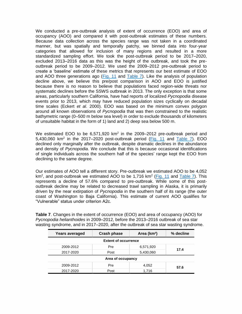
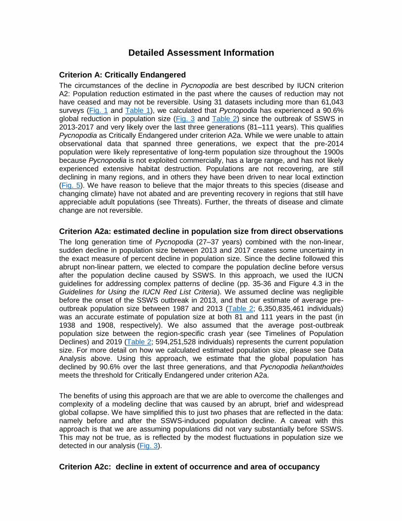
We conducted a pre-outbreak analysis of extent of occurrence (EOO) and area of occupancy (AOO) and compared it with post-outbreak estimates of these numbers. Because data collection across the species range was not taken in a coordinated manner, but was spatially and temporally patchy, we binned data into four-year categories that allowed for inclusion of many regions and resulted in a more standardized sampling effort. We took the post-outbreak period to be 2017‒2020, excluded 2013‒2016 data as this was the height of the outbreak, and took the pre-outbreak period to be 2009‒2012. We used the 2009‒2012 pre-outbreak period to create a ‘baseline’ estimate of these metrics that represents our best estimate of EOO and AOO three generations ago (Fig. 11 and Table 7). Like the analysis of population decline above, we believe this pre/post comparison in AOO and EOO is justified because there is no reason to believe that populations faced region-wide threats nor systematic declines before the SSWS outbreak in 2013. The only exception is that some areas, particularly southern California, have had reports of localized Pycnopodia disease events prior to 2013, which may have reduced population sizes cyclically on decadal time scales (Eckert et al. 2000). EOO was based on the minimum convex polygon around all known observations of Pycnopodia that was then constrained to the realistic bathymetric range (0‒500 m below sea level) in order to exclude thousands of kilometers of unsuitable habitat in the form of 1) land and 2) deep sea below 500 m.
We estimated EOO to be 6,571,920 km2 in the 2009‒2012 pre-outbreak period and 5,430,060 km2 in the 2017‒2020 post-outbreak period (Fig. 11 and Table 7). EOO declined only marginally after the outbreak, despite dramatic declines in the abundance and density of Pycnopodia. We conclude that this is because occasional identifications of single individuals across the southern half of the species’ range kept the EOO from declining to the same degree.
Our estimates of AOO tell a different story. Pre-outbreak we estimated AOO to be 4,052 km2, and post-outbreak we estimated AOO to be 1,716 km2 (Fig. 11 and Table 7). This represents a decline of 57.6% compared to pre-outbreak. While some of this post-outbreak decline may be related to decreased trawl sampling in Alaska, it is primarily driven by the near extirpation of Pycnopodia in the southern half of its range (the outer coast of Washington to Baja California). This estimate of current AOO qualifies for “Vulnerable” status under criterion A2c.
Table 7. Changes in the extent of occurrence (EOO) and area of occupancy (AOO) for Pycnopodia helianthoides in 2009‒2012, before the 2013‒2016 outbreak of sea star wasting syndrome, and in 2017‒2020, after the outbreak of sea star wasting syndrome.
Years averaged Crash phase Area (km²) % decline
Extent of occurrence
2009-2012 Pre 6,571,920 17.4
2017-2020 Post 5,430,060
Area of occupancy
2009-2012 Pre 4,052 57.6
2017-2020 Post 1,716
Figure 11. Maps of the extent of occurrence of Pycnopodia helianthoides with inset examples of the area of occurrence for a) the four years immediately before (2009‒2012) and b) the four years after (2017‒2020) the sea star wasting syndrome outbreak.
Criterion A2e: decline due to disease
Pycnopodia meets this criterion because disease was the primary driver of all population declines detailed in criteria A2a and A2c.
Criterion B: Vulnerable
Overall, Pycnopodia meets the definition of “Vulnerable” under criterion B2. The area of occupancy (1,717 km2) meets the 2,000 km2 “Vulnerable” threshold for B2. Additionally, it meets subcriteria B2a and B2b, as the number of locations is estimated to be as low as one and no higher than 10, and because the species meets the definition for continuing decline (see justification below). Overall, Pycnopodia qualify as Vulnerable under criterion B2ab
Subcriterion B2
Subcriterion B2a: severe fragmentation and number of locations.
Pycnopodia does not meet the definition of severely fragmented. While in the southern half of its range, small remnant populations are likely fragmented, most of the remaining individuals exist in more continuously distributed populations across the northern half of the range. Additionally, its biology does not lend itself to severe fragmentation; Pycnopodia is a habitat generalist, its method of reproduction (broadcast spawning with a pelagic larval duration) has the potential for broad larval dispersal, and it has few barriers to dispersal.
Despite its large geographic extent, Pycnopodia does appear to have a limited number of locations (defined by IUCN as a geographically or ecologically distinct area in which a single threatening process can rapidly affect all occurrences of an ecosystem type). The primary threat to the species is SSWS, and it appears that all global Pycnopodia populations were affected by the disease. Thus, the minimum number of locations could be considered one, since the 2013‒2017 outbreak demonstrated that all populations of this species can be rapidly affected by SSWS in a short period of time. However, considering the species’ broad geographic range, the true number of locations could be higher. For example, it appears that the western Gulf of Alaska and the Aleutian islands may have been less affected by the disease. If some locales were unaffected, the number of locations could be >1. While our current lack of understanding of this species’ biology, ecology, and threats limits our ability to put an upper limit on the number of locations, the fact that all populations of this species appear to have been affected within a three-year period by SSWS suggests that the number of locations is likely less than 10. Overall, we believe that the number of locations could be as low as one, which meets the threshold of “Critically Endangered” under subcriterion B2a.
Subcriterion B2b: continuing decline
Similar to our calculations of population decline under criterion A2a, the long generation time of Pycnopodia (27–37 years) combined with the non-linear, sudden decline in population size between 2013 and 2017 creates some uncertainty in the exact measure of continuing decline. Further, the causative agent for SSWS is unknown so we have no way to test the health of surviving individuals. Importantly, however, we continue to see evidence of SSWS in Pycnopodia and other species (see Threats) and it is quite possible that expression of the disease will return, especially if it is driven by warm
temperature anomalies associated with climate change. We believe this alone justifies a prediction of continued decline in the regions that still have remnant populations.
In addition, we analysed trends in population density since SSWS abated (Fig. 5; from 2017-2019) and found that the global population exhibits a weak negative trend. Further, upon investigating this trend among regions, we found that densities in regions on the outer coast of the contiguous United States and Mexico, have “flat lined” at extremely low densities (Fig. 5; Washington outer coast, Oregon, North, Central, Southern and Baja California). The regions with remaining populations, including much of Alaska and British Columbia (including the Salish Sea), have exhibited continuing declines since 2017. These findings suggest that Pycnopodia populations are experiencing a continued decline, which qualifies them for criterion B2b.
Subcriterion B2c: extreme fluctuations
While we detected some fluctuations in population size (and presumably mature individuals) over the 32-year time frame, we believe that this species does not generally undergo extreme fluctuations. First, the peak population size we detected in 2014-2015 was likely due to increased sampling effort, and was not a true increase in population size (see Declines for more information). Second, this species is long-lived (up to 65 years by our estimates), and reaches maturity within a few years, so this indicates that there are no extreme fluctuations in mature individuals. We also did not detect extreme fluctuations in EOO or AOO and we do not think there are true subpopulations in this widespread species. Overall, Pycnopodia does not meet the threatened threshold of extreme fluctuations for criterion B2c.
Criterion C: not threatened
With a post-outbreak population size estimate of 594,251,528 individuals (Table 2) and a 2019 population size estimate of 80,627,721 (Fig. 3a), most of which are mature, Pycnopodia does not qualify for threatened (<1,000 mature individuals) under criterion C.
Criterion D: not threatened
Although the population size and area of extent of Pycnopodia have greatly decreased since the outbreak of SSWS in 2013, our best estimate of AOO and population size as of 2019 was 1,716 km2 and 80,627,721 individuals, respectively (Table 7 and Fig. 5a, respectively). These metrics are far above the thresholds of 20 km2 and 1,000 individuals, respectively, required by criterion D and thus this species does not qualify for listing under criterion D.
Criterion E: Data Deficient
Burgman and Possingham (2010) note that some of the characteristics of a high quality population viability analysis (PVA) include deep knowledge of the species’ biology, habitat preferences, dispersal capability, threats, individual and population-wide responses to those threats, and the risk posed by these threats in the future. Unfortunately, we have very limited information on most of these categories for Pycnopodia. The broad lack of understanding of Pycnopodia biology and ecology and of
the disease that severely impacted the species prevent any kind of mechanistic understanding of how this species may or may not rebound in coming decades.
Furthermore, we do not have the data available to do many traditional kinds of PVAs. For instance, in their overview of PVA Akçakaya and Sjögren-Gulve (2000) note that three of the most common kinds of PVA are meta-population occupancy models, structured population models, and individual-based models. While we have the presence/absence data needed for an occupancy model, occupancy models typically are only used for highly spatially structured metapopulations and thus are not applicable to Pycnopodia. Structured population models and individual-based models require at a minimum age-specific or stage-specific information on mortality and reproduction, which is not available for Pycnopodia. The only kind of PVA we are aware of that we might be able to use are time-series analysis, such as the kind used in Dennis et al. (1991) and Holmes and Fagan (2002). However, these analyses usually require regular censuses of species’ population size, whereas the available population data on Pycnopodia are spatially limited and temporally patchy. Without a robust population time series or more detailed physiological, ecological, and epidemiological understanding of Pycnopodia, we do not think it is useful to conduct a PVA for this species’ assessment.
References Aalto, E.A., Lafferty, K.D., Sokolow, S.H., Grewelle, R.E., Ben-Horin, T., Boch, C.A.,
Raimondi, P.T., Bograd, S.J., Hazen, E.L., Jacox, M.G., Micheli, F. and De Leo, G.A. 2020. Models with environmental drivers offer a plausible mechanism for the rapid spread of infectious disease outbreaks in marine organisms. Scientific Reports 10(1): 1-10. https://doi.org/10.1038/s41598-020-62118-4
Akçakaya, H.R. and Sjögren-Gulve, P. 2000. Population viability analyses in conservation planning: an overview. Oikos 48: 9–21.
Altizer, S., Ostfeld, R.S., Johnson, P.T.J.J., Kutz, S. and Harvell, C.D. 2013. Climate change and infectious diseases: from evidence to a predictive framework. Science 341(6145): 514–519. https://doi.org/10.1126/science.1239401
Bates, A.E., Hilton, B.J. and Harley, C.D.G. (2009). Effects of temperature, season and locality on wasting disease in the keystone predatory sea star Pisaster ochraceus. Diseases of Aquatic Organisms 86(3): 245–251. https://doi.org/10.3354/dao02125
Bivand, R.S., Pebesma, E. and Gomez-Rubio, V. 2013. Applied spatial data analysis with R, Second edition. Springer, NY. https://asdar-book.org/
Bivand, R. and Rundel, C. 2020. rgeos: Interface to geometry engine - open source('GEOS'). R package version 0.5-3. https://CRAN.R-project.org/package=rgeos
Bivand, R., Keitt, T. and Barry Rowlingson, B. 2020. rgdal: Bindings for the 'Geospatial' data abstraction library. R package version 1.5-12. https://CRAN.R-project.org/package=rgdal
Bonaviri, C., Graham, M., Gianguzza, P. and Shears, N.T. 2017. Warmer temperatures reduce the influence of an important keystone predator. Journal of Animal Ecology 86(3): 490–500. https://doi.org/10.1111/1365-2656.12634
Bos, A.R., Gumanao, G.S., Alipoyo, J.C.E. and Cardona, L.T. 2008. Population dynamics, reproduction and growth of the Indo-Pacific horned sea star,
Protoreaster nodosus (Echinodermata; Asteroidea). Marine Biology 156(1): 55–63. https://doi.org/10.1007/s00227-008-1064-2
Burgman, M. and Possingham, H. 2010. Population viability analysis for conservation: the good, the bad and the undescribed. In: Genetics, Demography and Viability of Fragmented Populations, pp. 97–112. Cambridge University Press. https://doi.org/10.1017/cbo9780511623448.008
Burt, J.J.M., Tinker, T., Okamoto, D.K.D., Demes, K.W.K., Holmes, K. and Salomon, A.K.A. 2018. Sudden collapse of a mesopredator reveals its complementary role in mediating rocky reef regime shifts. Proceedings of the Royal Society B-Biological Sciences 285(1883). https://doi.org/10.1098/rspb.2018.0553
Dennis, B., Munholland, P.L. and Scott, J.M. 1991. Estimation of Growth and Extinction Parameters for Endangered Species. Ecological Monographs 61(2): 115-143.
DFO. (2019). Canada’s marine protected and conserved areas. Retrieved June 11, 2020, from https://www.dfo-mpo.gc.ca/oceans/conservation/areas-zones/index-eng.html
Duggins, D. 1983. Starfish predation and the creation of mosaic patterns in a kelp-dominated community. Ecology 64(6): 1610–1619. Retrieved from http://www.jstor.org/stable
Dungan, M., Miller, T. and Thompson, D. 1982. Catastrophic decline of a top carnivore in the Gulf of California rocky intertidal zone. Science 216(4549): 989–991.
Ebert, T.A. and Russell, M.P. 1992. Growth and mortality estimates for red sea urchin Strongylocentrotus franciscanus from San Nicolas Island, California. Marine Ecology Progress Series 81(1): 31–41. https://doi.org/10.3354/meps081031
Eckert, G.L. 2007. Spatial patchiness in the sea cucumber Pachythyone rubra in the California Channel Islands. Journal of Experimental Marine Biology and Ecology 348(1–2): 121–132. https://doi.org/10.1016/j.jembe.2007.04.004
Eckert, G.L., Engle, J.M. and Kushner, D.J. 1998. Sea star disease and population declines at the Channel Islands. Proceedings of the 5th California Island Symposium 5, 390–393.
Eisaguirre, J.H., Eisaguirre, J.M., Davis, K., Carlson, P.M., Gaines, S.D. and Caselle, J.E. 2020. Trophic redundancy and predator size-class structure drive differences in kelp forest ecosystem dynamics. Ecology 101(5): https://doi.org/10.1002/ecy.2993
Eisenlord, M.E., Groner, M.L., Yoshioka, R.M., Elliott, J., Maynard, J., Fradkin, S., Turner, M., Pyne, K., Rivlin, N., van Hooidonk, R. and Harvell, C.D. 2016. Ochre star mortality during the 2014 wasting disease epizootic: role of population size structure and temperature. Philosophical Transactions of the Royal Society of London B: Biological Sciences 371(1689): https://doi.org/10.1098/rstb.2015.0212
Feder, H.M. and Christensen, A.M. 1966. Aspects of asteroid biology. In: R. Boolootian (ed.) Physiology of Echinodermata pp. 87–127. Interscience Publishers, New York.
Gehman, A.-L.M., Hall, R.J. and Byers, J.E. 2018. Host and parasite thermal ecology jointly determine the effect of climate warming on epidemic dynamics. Proceedings of the National Academy of Sciences of the United States of America 115(4): https://doi.org/10.1073/pnas.1705067115
Giese, A.C., Pearse, J.S. and Pearse, V.B. 1991. Reproduction of marine invertebrates. Volume 6: Echinoderms and Lophophorates. Blackwell Scientific Publications, New York.
Gooding, R.A., Harley, C.D.G. and Tang, E. 2009. Elevated water temperature and carbon dioxide concentration increase the growth of a keystone echinoderm. Proceedings of the National Academy of Sciences of the United States of America 106(23): 9316–9321. https://doi.org/10.1073/pnas.0811143106
Greer, D. 1962. Studies on the embryology of Pycnopodia helianthoides (Brandt) Stimpson. Pacific Science 16(3): 280–285.
Harvell, C. D., Montecino-Latorre, D., Caldwell, J.M., Burt, J.M., Bosley, K., Keller, A., Heron, S.F., Salomon, A.K., Lee, L., Pontier, O., Pattengill-Semmens, C. and Gaydos, J.K. 2019. Disease epidemic and a marine heat wave are associated with the continental-scale collapse of a pivotal predator (Pycnopodia helianthoides). Science Advances 5(1): 1–9. https://doi.org/10.1126/sciadv.aau7042
Harvell, C. Drew, Mitchell, C.E., Ward, J.R., Altizer, S., Dobson, A.P., Ostfeld, R.S. and Samuel, M.D. 2002. Climate warming and disease risks for terrestrial and marine biota. Science 296(5576): 2158–2162. https://doi.org/10.1126/science.1063699
Herrlinger, T.J. 1983. The diet and predator-prey relationships of the sea star Pycnopodia helianthoides (Brandt) from a central California kelp forest. Thesis, San Jose State University.
Hewson, I., Bistolas, K.S.I., Quijano Cardé, E.M., Button, J.B., Foster, P.J., Flanzenbaum, J.M., Kocian, J. and Lewis, C.K. 2018. Investigating the complex association between viral ecology, environment, and northeast pacific sea star wasting. Frontiers in Marine Science 5: 77. https://doi.org/10.3389/fmars.2018.00077
Hewson, I., Button, J.B., Gudenkauf, B.M., Miner, B., Newton, A.L., Gaydos, J.K., Wynne, J., Groves, C.L., Hendler, G., Murray, M., Fradkin, S., Breitbart, M., Fahsbender, E., Lafferty, K.D., Kilpatrick, A.M., Miner, C.M., Raimondi, P., Lahner, L., Friedman, C.S., Daniels, S., Haulena, M., Marliave, J., Burge, C.A., Eisenlord, M.E. and Harvell, C.D. 2014. Densovirus associated with sea-star wasting disease and mass mortality. Proceedings of the National Academy of Sciences of the United States of America 111(48): 17278–17283. https://doi.org/10.1073/pnas.1416625111
Hewson, I., Sullivan, B., Jackson, E.W., Xu, Q., Long, H., Lin, C., Quijano Cardé, E.M., Seymour, J., Siboni, N., Jones, M.R.L. and Sewell, M.A. 2019. Perspective: something old, something new? Review of wasting and other mortality in Asteroidea (Echinodermata). Frontiers in Marine Science 6(July): 1–8. https://doi.org/10.3389/fmars.2019.00406
Hijmans, R.J. 2020. raster: Geographic data analysis and modeling. R package version 3.3-13. https://CRAN.R-project.org/package=raster
Holmes, E.E. and Fagan, W.F. 2002. Validating population viability analysis for corrupted data sets. Reports Ecology 83.
JMP Pro®, Version 14.2.0. SAS Institute Inc., Cary, NC, 1989-2019.
Keesing, J.K. 2017. Population size structure, growth, arm number and damage in the sea star Archaster angulatus (Müller and Troschel), 1842 (Echinodermata: Asteroidea). Invertebrate Reproduction and Development 61(2): 119–127. https://doi.org/10.1080/07924259.2017.1287782
Kirk, D., Luijckx, P., Stanic, A. and Krkošek, M. 2019. Predicting the thermal and allometric dependencies of disease transmission via the metabolic theory of ecology. The American Naturalist 193(5): 661–676. https://doi.org/10.1086/702846
Kohl, W.T., McClure, T.I. and Miner, B.G. 2016. Decreased temperature facilitates short-term sea star wasting disease survival in the keystone intertidal sea star Pisaster ochraceus. PLoS ONE 11(4): 1–9. https://doi.org/10.1371/journal.pone.0153670
Konar, B., Mitchell, T.J., Iken, K., Coletti, H., Dean, T., Esler, D., Lindeberg, M., Pister, B. and Weitzman, B. 2019. Wasting disease and static environmental variables drive sea star assemblages in the Northern Gulf of Alaska. Journal of Experimental Marine Biology and Ecology 520(July): 151209. https://doi.org/10.1016/j.jembe.2019.151209
Lucas, J. 1984. Growth, maturation and effects of diet in Acanthaster planci (L.) (Asteroidea) and hybrids reared in the laboratory. Marine Biology and Ecology 79(2): 129–147.
Lundquist, C.J. and Botsford, L.W. 2004. Model projections of the fishery implications of the Allee effect in broadcast spawners. Ecological Applications 14(3): 929–941. https://doi.org/10.1890/02-5325
Mauzey, K.P., Birkeland, C. and Dayton, P.K. 1968. Feeding behavior of asteroids and escape responses of their prey in the Puget Sound region. Ecology 49(4): 603–619.
Menge, B.A. 1975. Brood or broadcast? The adaptive significance of different reproductive strategies in the two intertidal sea stars Leptasterias hexactis and Pisaster ochraceus. Marine Biology 31(1): 87–100. https://doi.org/10.1007/BF00390651
Menge, B.A., Cerny-Chipman, E.B., Johnson, A., Sullivan, J., Gravem, S. and Chan, F. 2016. Sea star wasting disease in the keystone predator Pisaster ochraceus in Oregon: insights into differential population impacts, recovery, predation rate, and temperature effects from long-term research. PLoS One 11(5): e0153994. https://doi.org/10.1371/journal.pone.0153994
Miner, C.M., Burnaford, J.L., Ambrose, R.F., Antrim, L., Bohlmann, H., Blanchette, C.A., Engle, J.M., Fradkin, S.C., Gaddam, R., Harley, C.D. Miner, B.G., Murray, S.N., Smith, J.R., Whitaker, S.G. and Raimondi, P.T. 2018. Large-scale impacts of sea star wasting disease (SSWD) on intertidal sea stars and implications for recovery. PLoS ONE, 13(3): 1–21. https://doi.org/10.1371/journal.pone.0192870
Montecino-Latorre, D., Eisenlord, M.E., Turner, M., Yoshioka, R., Drew Harvell, C., Pattengill-Semmens, C.V., Nichols, J.D. and Gaydos, J.K. 2016. Devastating transboundary impacts of sea star wasting disease on subtidal asteroids. PLoS ONE 11(10): 1–14. https://doi.org/10.1371/journal.pone.0163190
Mordecai, E.A., Caldwell, J.M., Grossman, M.K., Lippi, C.A., Johnson, L.R., Neira, M., Rohr, J.R., Ryan, S.J., Savage, V., Shocket, M.S., Sippy, R., Stewart Ibarra, A.M., Thomas, M.B. and Villena, O. (2019, October 1). Thermal biology of mosquito-borne disease. Ecology Letters. Blackwell Publishing Ltd. https://doi.org/10.1111/ele.13335
Morris, R.H., Abbott, D.P. and Haderlie, E.C. (eds) 1980. Intertidal Invertebrates of California: Asteroidea. Stanford, CA: Stanford University Press.
NOAA. 2020. National MPA Center. Retrieved June 1, 2020, from https://marineprotectedareas.noaa.gov/aboutmpas/mpacenter/
Pebesma, E.J. and Bivand, R.S. 2005. Classes and methods for spatial data in R. R News 5 (2): https://cran.r-project.org/doc/Rnews/
R Development Core Team. 2008 R: a language and environment for statistical computing. R Foundation for Statistical Computing, Vienna.
Rassweiler, A., Schmitt, R.J. and Holbrook, S.J. 2010. Triggers and maintenance of multiple shifts in the state of a natural community. Oecologia 164(2): 489–498. https://doi.org/10.1007/s00442-010-1666-5
Rogers-Bennett, L. and Catton, C.A. 2019. Marine heat wave and multiple stressors tip bull kelp forest to sea urchin barrens. Nature 9(15050): 1–9. https://doi.org/10.1038/s41598-019-51114-y
Rogers-Bennett, L., Rogers, D.W., Bennett, W.A. and Ebert, T.A. 2003. Modeling red sea urchin (Strongylocentrotus franciscanus) growth using six growth functions. Fishery Bulletin 101(3): 614–626.
Schultz, J.A., Cloutier, R.N. and Côté, I.M. 2016. Evidence for a trophic cascade on rocky reefs following sea star mass mortality in British Columbia. PeerJ 4(4): e1980. https://doi.org/10.7717/peerj.1980
Sebens, K.P. 1987. The ecology of indeterminate growth in animals. Annual Review of Ecology and Systematics 18: 371–407. https://doi.org/10.1111/j.1751-0813.1981.tb00545.x
Sewell, M. and Watson, J.C. 1993. A “source” for asteroid larvae?: Recruitment of Pisaster ochraceus, Pycnopodia helianthoides and Dermasterias imbricata in Nootka Sound, British Columbia. Marine Biology 117: 387–398.
Staehli, A., Schaerer, R., Hoelzle, K. and Ribi, G. 2009. Temperature induced disease in the starfish Astropecten jonstoni. Marine Biodiversity Records 2: e78. https://doi.org/10.1017/S1755267209000633
Strathmann, R.R. 1978. The evolution and loss of feeding larval stages of marine invertebrates. Evolution 32(4): 894–906. Retrieved from https://www.jstor.org/stable/2407502
Wilmes, J., Matthews, S., Schultz, D., Messmer, V., Hoey, A. and Pratchett, M. 2017. Modelling growth of Juvenile crown-of-thorns starfish on the northern Great Barrier Reef. Diversity 9(1): 1–11. https://doi.org/10.3390/d9010001
Yamaguchi, M. 1974. Growth of juvenile Acanthaster planci (L.) in the laboratory. Pacific Science 28(2): 123–138.