structural properties of the mastoid using image...
TRANSCRIPT

Linköping Studies in Science and TechnologyDissertations, No. 1862
Structural properties of the mastoidusing image analysis and visualization
Olivier Cros
Department of Biomedical EngineeringLinköping University, Sweden
Linköping, June 2017
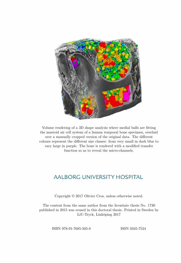
Volume rendering of a 3D shape analysis where medial balls are fittingthe mastoid air cell system of a human temporal bone specimen, overlaid
over a manually cropped version of the original data. The differentcolours represent the different size classes: from very small in dark blue to
vary large in purple. The bone is rendered with a modified transferfunction so as to reveal the micro-channels.
Copyright © 2017 Olivier Cros, unless otherwise noted.
The content from the same author from the licentiate thesis No. 1730published in 2015 was reused in this doctoral thesis. Printed in Sweden by
LiU-Tryck, Linköping 2017
ISBN 978-91-7685-505-8 ISSN 0345-7524

Abstract
The mastoid, located in the temporal bone, houses an air cell system whosecells have a variation in size that can go far below current conventionalclinical CT scanner resolution. Therefore, the mastoid air cell system is onlypartially represented in a clinical CT scan. Where the conventional clinicalCT scanner lacks level of minute details, micro-CT scanning provides anoverwhelming amount of fine details. The temporal bone being one of themost complex in the human body, visualization of micro-CT scanning ofthis bone awakens the curiosity of the experimenter, especially with thecorrect visualization settings.
This thesis first presents a statistical analysis determining the surface areato volume ratio of the mastoid air cell system of human temporal bone, frommicro-CT scanning using methods previously applied for conventional clin-ical CT scans. The study compared current results with previous studies,with successive downsampling the data down to a resolution found in con-ventional clinical CT scans. The results from the statistical analysis showedthat all the small mastoid air cells, that cannot be detected in conventionalclinical CT scans, do heavily contribute to the estimation of the surfacearea, and in consequence to the estimation of the surface area to volumeratio by a factor of about 2.6. Such a result further strengthens the idea ofthe mastoid to play an active role in pressure regulation and gas exchange.
Discovery of micro-channels through specific use of a non-traditional trans-fer function was then reported, where a qualitative and a quantitative pre-analysis were performed and reported. To gain more knowledge about thesemicro-channels, a local structure tensor analysis was applied where struc-tures are described in terms of planar, tubular, or isotropic structures. Theresults from this structural tensor analysis suggest these micro-channelsto potentially be part of a more complex framework, which hypotheticallywould provide a separate blood supply for the mucosa lining the mastoidair cell system.
The knowledge gained from analysing the micro-channels as locally provid-ing blood to the mucosa, led to the consideration of how inflammation ofthe mucosa could impact the pneumatization of the mastoid air cell sys-tem. Though very primitive, a 3D shape analysis of the mastoid air cellsystem was carried out. The mastoid air cell system was first representedin a compact form through a medial axis, from which medial balls could beused. The medial balls, representative of how large the mastoid air cells canbe locally, were used in two complementary clustering methods, one based

iv
on the size diameter of the medial balls and one based on their locationwithin the mastoid air cell system. From both quantitative and qualita-tive statistics, it was possible to map the clusters based on pre-definedregions already described in the literature, which opened the door for newhypotheses concerning the effect of mucosal inflammation on the mastoidpneumatization.
Last but not least, discovery of other structures, previously unreportedin the literature, were also visually observed and briefly discussed in thisthesis. Further analysis of these unknown structures is needed.

Acknowledgements
Many people have contributed to this thesis, directly or indirectly. First, Iam grateful for my employer, the department of Otolaryngology, Head andNeck Surgery, at Aalborg Hospital South in Aalborg, Denmark. Withoutthe financial support and great patience, I would not be here today.
I would like to particularly thank MD & PhD Michael Gaihede, my mainclinical supervisor, for your constant support and providing this amazingknowledge you have about the ear both from an anatomical but also froma physiological point of view. Simona, you are not forgotten either, I hopeyou will keep up the hard work.
I would also like to thank Professor Hans Knutsson, my main technicalsupervisor, for being the source of many ideas and inspiration. Thank youalso Dr. Mats Andersson for endless discussions about other things thanwork, and motivating me during tough periods from personal matters butalso when in doubt with my academic career. Also big thanks to Dr. AndersEklund, my co-supervisor, for your already endless support and our dailytalks.
Thank you Professor Magnus Borga for your early supervision. Also, thanksto my colleagues and the staff at the department of biomedical engineeringfor always being kind and helpful, especially Göran Salerud. Thank youfor having me so long.
I would also like to acknowledge the people at the centre for X-ray Tomogra-phy, Department of Physics and Astronomy, University of Ghent, Belgium;especially Elin Pawels and Manuel Dierick and their colleagues. Withoutyou, this PhD would definitely have turned in a different direction.
I also want to greet my friends, especially Anders Eklund, Peter Remjstad,Maria Ewerlöf, Filipe Marreiros, Patrick Bennysson, Rafael Sanchez with-out whom I would have felt quite alone on the daily basis. You have beena great support directly and indirectly.
All my gratitudes to my family, especially my parents Jacques and NicoleCros, for always being supportive and engaged in my research. Withoutyou I would not be where I am. Mum and Dad, I hope you are in peacewhere you are now, and I miss you terribly. You have no idea how much Ilearned from you two and I stil carry your principles in me. Thanks to my

vi
both sisters Nathalie Pesson and Véronique Poupon and their respectivefamilies.
Mum, thanks to you, I met my beautiful fiancé and future wife ÉlodieDebiez and despite the fact that you and dad will never meet her, I amsure you would have adopted her right away. Thank you mum for this lastbut very important gift in life.
Élodie Debiez, thank you for your moral support and your positivism whenI most needed it. Thank you Marie Debiez for integrating me in your sweetfamily. I know that it has been a very tough period for you and me Élodie,but because we have been there for each others, we got stronger than ever.And looking at the future, I also know we will have beautiful moments. Weboth lost important people in our life, but we also gained someone in lifeand maybe more. I have no other words than Je t’aime!
Olivier Cros.
Linköping, June 2017.

Table of Contents
1 Introduction 11.1 Foreword . . . . . . . . . . . . . . . . . . . . . . . . . . . . 11.2 Thesis outline . . . . . . . . . . . . . . . . . . . . . . . . . . 21.3 Publications . . . . . . . . . . . . . . . . . . . . . . . . . . . 41.4 Related Publications . . . . . . . . . . . . . . . . . . . . . . 51.5 Abbrevations . . . . . . . . . . . . . . . . . . . . . . . . . . 61.6 Acronyms . . . . . . . . . . . . . . . . . . . . . . . . . . . . 6
2 General Anatomy & Physiology 72.1 Introduction . . . . . . . . . . . . . . . . . . . . . . . . . . . 72.2 Anatomy of the temporal bone . . . . . . . . . . . . . . . . 8
2.2.1 Outer ear . . . . . . . . . . . . . . . . . . . . . . . . 92.2.2 Middle ear . . . . . . . . . . . . . . . . . . . . . . . 102.2.3 Inner ear . . . . . . . . . . . . . . . . . . . . . . . . 112.2.4 Eustachian tube . . . . . . . . . . . . . . . . . . . . 13
3 The Mastoid 173.1 Introduction . . . . . . . . . . . . . . . . . . . . . . . . . . . 173.2 Development process . . . . . . . . . . . . . . . . . . . . . . 173.3 After birth development . . . . . . . . . . . . . . . . . . . . 183.4 Origin of the mastoid air cells in the newborns . . . . . . . 183.5 The adult mastoid . . . . . . . . . . . . . . . . . . . . . . . 213.6 Level of pneumatization . . . . . . . . . . . . . . . . . . . . 233.7 Pressure regulation and gas exchange . . . . . . . . . . . . . 243.8 Inflammation of the mucosa lining the air cells . . . . . . . 273.9 Otitis media . . . . . . . . . . . . . . . . . . . . . . . . . . . 30
4 Imaging Modalities 314.1 Introduction . . . . . . . . . . . . . . . . . . . . . . . . . . . 314.2 Clinical X-ray CT scanner . . . . . . . . . . . . . . . . . . . 334.3 Cone-Beam CT scanner . . . . . . . . . . . . . . . . . . . . 354.4 Histological sections . . . . . . . . . . . . . . . . . . . . . . 364.5 Micro-CT scanner . . . . . . . . . . . . . . . . . . . . . . . 39
5 Observations from the data and aims of the thesis 435.1 Introduction . . . . . . . . . . . . . . . . . . . . . . . . . . . 435.2 Midline of the mastoid air cell system . . . . . . . . . . . . 43

viii Table of Contents
5.3 What is a mastoid air cell in terms of shape? . . . . . . . . 445.4 What is the size of an air cell? . . . . . . . . . . . . . . . . 475.5 Air-mucosa versus mucosa-bone surface area . . . . . . . . . 475.6 Discovery of micro-channels . . . . . . . . . . . . . . . . . . 495.7 Aims of the thesis . . . . . . . . . . . . . . . . . . . . . . . 50
6 Image Processing 536.1 Introduction . . . . . . . . . . . . . . . . . . . . . . . . . . . 53
6.1.1 Segmentation by thresholding . . . . . . . . . . . . . 536.1.2 Morphology on binary images . . . . . . . . . . . . . 556.1.3 Masking original data over a binary segmentation . . 596.1.4 Measuring surface area and volume . . . . . . . . . . 60
6.2 More advanced image processing . . . . . . . . . . . . . . . 626.2.1 Filter design . . . . . . . . . . . . . . . . . . . . . . 646.2.2 The quadrature filter . . . . . . . . . . . . . . . . . . 716.2.3 Tensor analysis . . . . . . . . . . . . . . . . . . . . . 756.2.4 Extraction of planar, tubular, and isotropic structures 76
6.3 Enhancement through adaptive filtering . . . . . . . . . . . 796.4 Volume rendering . . . . . . . . . . . . . . . . . . . . . . . . 87
6.4.1 Multiple volume renderings . . . . . . . . . . . . . . 90
7 3D Shape Analysis 977.1 Introduction . . . . . . . . . . . . . . . . . . . . . . . . . . . 977.2 General definition of a shape . . . . . . . . . . . . . . . . . 987.3 Euclidean distance transform . . . . . . . . . . . . . . . . . 1037.4 Skeletonization . . . . . . . . . . . . . . . . . . . . . . . . . 1057.5 Medial surface . . . . . . . . . . . . . . . . . . . . . . . . . 1097.6 Medial axis . . . . . . . . . . . . . . . . . . . . . . . . . . . 1127.7 Medial balls . . . . . . . . . . . . . . . . . . . . . . . . . . . 1137.8 K-means clustering . . . . . . . . . . . . . . . . . . . . . . . 1147.9 Convex hull . . . . . . . . . . . . . . . . . . . . . . . . . . . 1157.10 Clustering the air cells . . . . . . . . . . . . . . . . . . . . . 116
7.10.1 Clustering in relation to size . . . . . . . . . . . . . 1167.10.2 Clustering in relation to 3D location . . . . . . . . . 120
8 Summary of Papers 1278.1 Introduction . . . . . . . . . . . . . . . . . . . . . . . . . . . 1278.2 Paper I . . . . . . . . . . . . . . . . . . . . . . . . . . . . . 1288.3 Paper II . . . . . . . . . . . . . . . . . . . . . . . . . . . . . 1288.4 Paper III . . . . . . . . . . . . . . . . . . . . . . . . . . . . 1298.5 Paper IV . . . . . . . . . . . . . . . . . . . . . . . . . . . . 1298.6 Paper V . . . . . . . . . . . . . . . . . . . . . . . . . . . . . 1308.7 Paper VI . . . . . . . . . . . . . . . . . . . . . . . . . . . . 130

Table of Contents ix
9 Discussion & Conclusion 1319.1 Fulfillment of the aims or not? . . . . . . . . . . . . . . . . 131
9.1.1 Geometrical aspects of mastoid air cell system . . . 1319.1.2 Interpretation and geometrical description of the dis-
covered micro-channels . . . . . . . . . . . . . . . . . 1369.2 Future methodological aspects to consider . . . . . . . . . . 139
9.2.1 Clinical aspects . . . . . . . . . . . . . . . . . . . . . 1399.2.2 Technical aspects . . . . . . . . . . . . . . . . . . . . 143
9.3 Strands and membranes within the MACS . . . . . . . . . . 1489.4 Pores in the septae . . . . . . . . . . . . . . . . . . . . . . . 1509.5 Bone spicules . . . . . . . . . . . . . . . . . . . . . . . . . . 1529.6 Conclusion . . . . . . . . . . . . . . . . . . . . . . . . . . . 154


1Introduction
1.1 Foreword
Similarly to the lungs, the rate of gas exchange carried out by the mastoidprocess in the temporal bone is determined by the mucosal surface area [64].This is particularly the case for the mastoid bone with its complex air cellsystem, with cells of varying sizes and shapes. An impaired gas exchange,besides a malfunctioning Eustachian tube, results in a negative middle earpressure; i.e. both in the tympanum and in the mastoid air cell system.Negative middle ear pressure leads to different middle ear diseases, such asthe otitis media with effusion, cholesteatoma invading all the airspaces inthe middle ear, or retraction pockets in the tympanum [62]. As stated in[19], understanding the mechanism of the middle ear pressure regulation isimportant for both physiologists and practising clinicians; especially for thepractising clinicians in their decisions on how to treat their patients. Thesurface area of the mucosa in the middle ear, especially the one covering themastoid air cell system, is therefore a valuable parameter for physiologicalstudies of gas exchanged between the air cells and the capillaries present inthe mucosa lining the air cells [18, 19, 62].
Quantitative measurement of the entire mastoid air cell system aeration is,however, only reported in few studies [17, 64, 78]. A plausible explanationof this sparse literature emanates from the fact that there is no techniqueavailable to allow a direct measurement of the mucosa surface area for theentire mastoid air cell system in vivo. An alternative is to scan the mastoidbone through X-ray computed tomography (CT), and consider the walls ofthe mastoid air cell system as a surrogate to the very thin mucosa invisibleon clinical CT scans. The volume of gas occupied within the mastoid aircells, also important to estimate when investigating how well a mastoid ispneumatized, is though easier to estimate using X-ray CT and has beenreported in several studies [84, 17, 37, 48, 54, 64, 77, 88].

2 Chapter 1. Introduction
Recent advances in micro-CT scanning technology allows scanning suchcomplex structures using very high resolution, in turn producing more ac-curate statistics. The aim of this work is to investigate the use of micro-CTscanning of human temporal bone specimens, to estimate the surface areato volume ratio using classical image processing methods, to compare withresults from previous studies where conventional clinical CT scans wereused, and finally to assess whether the obtained estimates help to furtherunderstand the anatomy and physiology of the mastoid air cell system.
Micro-channels were discovered while visualizing the temporal bone spec-imens using different visualization settings. A structural analysis of themicro-channels within the bone was therefore assessed. The results fromthe structural analysis further suggested to enhance the original data byreducing the noise level to a minimum, while slightly enhancing their rep-resentation.
Inspired from the idea of the micro-channels forming a supplementary bloodsupply to the mucosa lining the mastoid air cell system, the last part ofthe study aimed at investigating how the diameter of the air cells, under-stood as the cell size, influence the level of pneumatization of the temporalbone, at the level of the mastoid air cell system during inflammation. Toachieve this aim, a compact representation of the mastoid air cell systemwas obtained through the use of a structure tensor analysis on a distancetransform computed from the enhanced data. A shape analysis was pos-sible through the use of a medial unit composed of a medial surface, amedial axis and medial balls. Clustering of the medial balls in terms of sizeand three-dimensional location could help investigate the size variation, butalso where each size class is located in the mastoid. Although the medialballs are not a direct representation of the mastoid air cells, their use in ashape analysis opens a new door into the analysis of the mastoid in termsof pneumatization, which is beyond the more conventional surface area andvolume estimations.
Overall, this thesis is an attempt to open new doors when analyzing themastoid air cell system using image analysis while using micro-CT scans.
1.2 Thesis outline
The thesis is divided into nine parts. The thesis is formed in a way suchthat non-medical readers can obtain a brief and basic introduction to theanatomy and physiology of the human temporal bone in Chapter 2, andobtain more information about the mastoid process alone in Chapter 3.Chapter 4 gives a brief description of the image modalities often used wheninvestigating the mastoid, from conventional clinical CT scanner up to his-tological sections, together with the image modality that was used to pro-

1.2 Thesis outline 3
duce the high resolution scans, i.e. X-ray micro-CT. This chapter can beof interest for both clinical and technical readers who are not so familiarwith the different modalities. Chapter 5 states the aims for this overallwork based on observations made from the micro-CT scans supported byhistological sections at some occasions. For non-technical readers, chapter6 introduces some necessary concepts in image processing. The second halfof chapter 6 describes a method used forms the basis for Papers III, V, VI,and VII. Chapter 7 is devoted to a 3D shape analysis and stands on its owndue to the use of tools that belong more to discrete geometry and patternrecognition than image processing. Chapter 8 summarises the contributionof each paper. Chapter 9 provides a discussion about the presented workand ideas for future work, followed by a section illustrating the presence ofmucosal strands in the mastoid air cell system which has not been foundin previous literature. Two unpublished anatomical findings more relatedto the bone than soft tissues, are also reported.
N.B.: It should be noted that besides Figs. 2.4, 2.5, 2.6, 2.7, 2.8, 2.9,3.1, 4.5, 4.6, 4.7, 5.6, 9.3, all remaining illustrations presented in thisthesis were produced by the sole author Olivier Cros. Permission to usethese illustrated should be asked beforehand. Moreover, some illustrationsare from the sole author but were published in some of the papers. Fig. 5.1is published in Paper V and therefore permission to use this illustration hasto be granted by IEEE. Fig. 6.29 is published in Paper VI and therefore per-mission to use this illustration has to be granted by IEEE. Figs. 3.5, 7.10,7.15, 7.19, and 7.22 are submitted in Paper VII and therefore permissionto use this illustration has to be granted by Elsevier.

4 Chapter 1. Introduction
1.3 Publications
I Olivier Cros, Hans Knutsson, Mats Andersson, Elin Pawels, MagnusBorga, Michael Gaihede. Determination of the mastoid surface areaand volume based on micro-CT scanning of human temporal bones.Geometrical parameters depend on scanning resolutions. Acceptedand published in the medical journal Hearing Research Special IssueMEMRO, Volume 340, pages 127-134, 2016.
II Olivier Cros, Magnus Borga, Elin Pawels, Joris JJ Dirckx, MichaelGaihede. Micro-channels in the mastoid anatomy. Indications ofa separate blood supply of the air cell system mucosa by micro-CTscanning. Accepted and published in the medical journal HearingResearch Special Issue MEMRO, Volume 301, pages 60-65, 2013.
III Olivier Cros, Michael Gaihede, Mats Andersson, Hans Knutsson.Structural analysis of micro-channels in human temporal bone. Ac-cepted for IEEE International Symposium on Biomedical Imaging(ISBI), New York, United States of America, pages 9-12, April 2015.
IV Olivier Cros, Anders Eklund, Michael Gaihede, Hans Knutsson En-hancement of micro-channels within the human mastoid bone basedon local structure tensor analysis. Accepted for IEEE sixth Inter-national Conference on Image Processing Theory, Tools and Applica-tions (IPTA’16), IEEE, Oulu, Finland, December 2016.
V Olivier Cros, Michael Gaihede, Anders Eklund, Hans Knutsson Sur-face and curve skeleton from a structure tensor analysis applied onmastoid air cells in human temporal bones. Accepted for IEEE In-ternational Symposium on Biomedical Imaging (ISBI), Melbourne,Australia, April 2017.
VI Olivier Cros, Anders Eklund, Michael Gaihede, Hans KnutssonLocal size descriptor of mastoid air cells in human temporal bonebased on a structure tensor analysis from an Euclidean distance trans-form. Submitted to the journal Computerized Medical Imaging andGraphics, March 2017.

1.4 Related Publications 5
1.4 Related Publications
I Gunnar Läthén G., Olivier Cros, Hans Knutsson, Magnus Borga.Non-ring filters for robust detection of linear structures. Note: littlecontribution. IEEE 20th International Conference on Pattern Recog-nition (ICPR), pp. 233-236, 2009.
II Olivier Cros, Hans Knutsson, Mats Andersson, Elin Pawels, MagnusBorga, Michael Gaihede. Mastoid structural properties determinedby analysis of high-resolution CT scanning. Note: medical abstract.Hearing Research, 263:1-2, pages 242-243, 2010.
6 Chapter 1. Introduction
1.5 Abbrevations
This list provides abbreviations used in this thesis, along with their mean-ings.
CT Computed TomographyMAC Mastoid Air CellMACS Mastoid Air Cell SystemME Middle earTYMP TympanumTM Tympanic membraneOM Otitis mediaEC Ear canalEDT Euclidean distance transformET Eustachian tubeSNR Signal to Noise Ratio
1.6 Acronyms
This list provides the different acronyms related to anatomical locations.
• Lateral towards the outside,• Medial towards the midline,• Anterior towards the front,• Posterior towards the back,• Superior towards the top,• Inferior towards the bottom,
• Endo- inner part of a structure,• Meso- middle part of a structure,• Ecto- outer part of a structure,• Exo- external to a structure,• Epi- outside a structure,• Hypo- under the structure,• Hyper- over the structure,• Inter- between structures,• Intra- within a structure,• Peri- surrounding a structure,• Retro- behind a structure.

2General Anatomy & Physiology
2.1 Introduction
Before introducing the temporal bone as a whole entity, taxonomy of anatom-ical terms and spatial positions is briefly introduced, with the six mostrelevant positions illustrated in Fig. 2.1, i.e. inferior, superior, posterior,anterior, medial and lateral. A list of acronyms is provided in Chapter 1.
Figure 2.1: Anatomical directions.
These terms are used alternatively, globally or locally. As a simple example,the temporal bone is located laterally in relation the human skull, while thecochlea is located medially in relation to the temporal bone. Combinationof locations are also possible as, for instance, the superior retrosigmoid air

8 Chapter 2. General Anatomy & Physiology
cells are located at the superior part and at the back of the mastoid process.A structure located at the periphery of another structure is for examplethe lateral perisinusal cells, referring to air cells at the periphery of a sinuslocated in the back of the mastoid towards the lateral side of the bone.As a side note, mastoid air cells located at the centre of the mastoid canalso be named medial or central air cells, while air cells located towards theoutside of the mastoid bone will be called lateral or peripheral air cells. Thisnotion should be kept in mind while reading the thesis. To further help thereader, taxonomy of the different terms used when describing a structureorientation in medical images is resumed in Section 1.6 and representedgraphically in Fig. 2.1.
2.2 Anatomy of the temporal bone
The temporal bone houses the organ of hearing. The temporal bone consistsof five parts: the temporal squamosa, the petrous portion, the mastoidprocess, the tympanic bone, and the styloid process, see Fig. 2.2.
Figure 2.2: The temporal bone viewed alone from a lateral side (left) and a medialside (right), respectively viewed from the outside and the inside.
The temporal squamosa (from Latin squama, "scale"-shape structure) is thebiggest part of the temporal bone, lying superior to all parts. The petrousportion of the temporal bone, located inside the skull, is recognizable withits pyramidal shapes housing the middle ear and the inner ear. The wordpetrous originates from the Latin word petrosus, and relates to the veryhard portion of the bone housing the internal auditory organs. The mastoidprocess, from the new Latin "mastoides" resembling a nipple or breast, islocated posteriorly and inferiorly to the squamous part.
The tympanic bone is a small portion situated inferior to the temporalsquamosa, anterior to the mastoid process, and superior to the styloid pro-cess. The styloid process runs inferior to the tympanic bone, and is shaped

2.2 Anatomy of the temporal bone 9
like a thorn pointing downwards. It is used as an anchor point for severalmuscles. The described structures are illustrated in Fig. 2.2. A coronalsection of a right temporal bone reveals the complexity inside the temporalbone, see Fig. 2.3.
Figure 2.3: Cut through a temporal bone to reveal all its internal structures.Source: Atlas of Skull Base Surgery & Neurotology, Thieme, 2009.Image copyrighted by RK Jackler. Permission granted for non-profiteducational use.
From a physiological point of view, the temporal bone can be decomposedinto three main parts: the external ear, the middle ear, and the innerear. These parts are described in the following sections.
2.2.1 Outer ear
The outer ear is the external portion of the ear, which consists of thepinna, the external auditory meatus (also known as the ear canal), and thetympanic membrane, see Fig. 2.4.
The pinna, also known as the auricle, is the visible portion that is generallyreferred to as "the ear". Its function is to localize sound sources and directsound into the ear. The folds of the pinna allow some specific frequenciesto be amplified, while other frequencies can be damped.
The external auditory meatus (EAM), also named the external audi-tory canal or simply the ear canal, extends from the pinna to the tympanicmembrane and has a length of about 26 millimetres (mm) and a diameterof about 7 mm. The size and shape of the ear canal vary among individualsand between the left and right ears.

10 Chapter 2. General Anatomy & Physiology
Figure 2.4: The outer ear. Legend EAM: external auditory maetus. Source:Atlas of Skull Base Surgery & Neurotology, Thieme, 2009. Imagecopyrighted by RK Jackler. Permission granted for non-profit edu-cational use.
The tympanic membrane, also known as the eardrum, is a cone-shapedstructure separating the outer ear from the middle ear and protects the mid-dle and inner ear from foreign objects. The tympanic membrane resonatesin response to sound pressure waves. The displacement during vibration isextremely small, about one-billionth of a centimetre.
2.2.2 Middle ear
The middle ear cavity is a combination of two cavities, the tympanum andthe mastoid air cell system. Since the mastoid will be described further,only the tympanum is briefly introduced. The tympanum is the narrowair-filled space of the middle ear, where the ossicles are located, see Fig.2.5. The tympanum resembles an oblique rectangular room with a floor, aceiling, and four walls. Sound waves traveling through the ear canal will hitthe tympanic membrane. This wave information travels across the air-filledtympanum via a series of delicate bones called the ossicles, see Fig. 2.6.The ossicles are composed of the malleus (also known as hammer), incus(also known as anvil) and stapes (also known as stirrup), see Fig. 2.6. Theyform an ossicular chain.
While the handle of the malleus, also known as the manubrium, articulateswith the tympanic membrane, the footplate of the stapes articulates withthe oval window, a membrane-covered opening which leads to the vestibule

2.2 Anatomy of the temporal bone 11
Figure 2.5: The tympanum, being part of the middle ear. Source: Atlas of SkullBase Surgery & Neurotogy, Thieme, 2009. Image copyrighted by RKJackler. Permission granted for non-profit educational use.
of the inner ear, located at the opposite side of the tympanum. Tendonsattaching the head of the malleus and the incus are attached to the tegmentympani, a bony wall separating the cranial cavity from the superior partof the tympanum, the epitympanic recess or attic, see the vertical tendonsin Fig. 2.6. Behind the head of the malleus and towards its upper part,the posterior wall of the tympanum is mostly occupied by the aditus adantrum, a path towards the mastoid air cell system via the antrum.
2.2.3 Inner ear
The inner ear, shown in Fig. 2.7, can be divided into two labyrinths: abony labyrinth and a membranous labyrinth.
The osseous labyrinth consists of the cochlea, the vestibule, and the semi-circular canals, a series of bony cavities within the petrous temporal bone.These bony cavities are lined with periosteum and contain perilymph; ex-tracellular fluid at the periphery of the structure. The oval window, artic-ulated by the footplate of the stapes, is an opening in the lateral wall ofthe vestibule of the osseous labyrinth.
The membranous labyrinth is composed of communicating membranoussacs and ducts housed within the osseous labyrinth. It is cushioned by thesurrounding perilymph and contains the endolymph within its confines; anextracellular fluid inside the structure. The membranous labyrinth also

12 Chapter 2. General Anatomy & Physiology
Figure 2.6: The ossicular chain with the malleus in direct contact with the tym-panic membrane, and the stapes viewed laterally attached to theoval window separating the vestibule from the tympanum. The incustransmits the movements induced by the malleus to the stapes. Also,notice the tendons attaching the ossicles to the tympanum. Source:Gray plate 919 made public available.
houses a cochlear, a vestibular, and semicircular canals components.
Cochlea
The cochlea is the auditory portion of the inner ear. The spiral-shapedcavity within the cochlea has three fluid-filled sections along its main axis:the scala vestibuli, the scala tympani, and the cochlear duct. The organof Corti, located in the cochlear duct on the basilar membrane, transformsmechanical waves into electric signals sent to the neurons in the brain.
Vestibule
The vestibule is the central part of the osseous labyrinth. The vestibularapparatus is composed of the utricle and the saccule. They respectivelysense linear acceleration in the horizontal and vertical planes. Within theseorgans are hair cells. The cilia of these cells are intricately associatedwith a membranous substance containing calcium carbonate granules, or"otoliths", also commonly known as stones in the cochlea. Movement ofthe head induces a shearing of the hair cells by the mobile otoliths. Thisdirectional change is sensed by the brain via the superior division of the

2.2 Anatomy of the temporal bone 13
Figure 2.7: The inner ear. Source: Atlas of Skull Base Surgery & Neurot-ogy, Thieme, 2009. Image copyrighted by RK Jackler. Permissiongranted for non-profit educational use.
vestibular nerve at the utricle, and via the inferior division of the vestibularnerve to the saccule. Together, the otolithic organ organs of both ears areof prime importance for directional sensation.
Semi-circular canals
The third main apparatus in the inner ear is the set of three semi-circularcanals. Each stands at right angles in relation to each others. The superior,posterior, and lateral semicircular canals are located posterior and superiorto the vestibule.
2.2.4 Eustachian tube
The Eustachian tube originates in the posterior part of the nose, runsslightly uphill, and enters the tympanum inferiorly, see Fig. 2.8 (left). Thecartilage provides a supporting structure for two thirds of the Eustachiantube, while the part closest to the tympanum is made of bone. The tissuelining the Eustachian tube is similar to that inside the nasal cavity, and mayrespond in the same way (swelling) when presented with similar stimuli.
Function of the Eustachian tube
The primary function of the Eustachian tube is to ventilate the middleear space, ensuring that its pressure remains at near normal environmental

14 Chapter 2. General Anatomy & Physiology
Figure 2.8: Course of the Eustachian tube from the middle ear (left) and itsentrance from the nasal cavity (right), see the red vertical arrow.Source: left. Hill, M.A. (2015) Embryology Gray0915.jpg, right: [1].
air pressure; known as middle ear pressure. The secondary function ofthe Eustachian tube is to drain any accumulated secretions, infections, ordebris from the tympanum.
Several small muscles located in the back of the throat and palate controlthe opening and closing of the tube. Swallowing and yawning cause con-tractions of the muscles located in the back of the throat, and facilitatethe regulation of the Eustachian tube function. If it was not for the Eu-stachian tube, the middle ear cavity would be an isolated air pocket insidethe head, which would be vulnerable to every change in air pressure, under-and over-pressure, leading to a pathological middle ear.
Normally, the Eustachian tube is closed, which helps to prevent the in-advertent contamination of the middle ear space by the normal secretionsfound in the back of the nose. A dysfunctional Eustachian tube can leadto chronic ear infections. A much more common problem is a failure of theEustachian tube to effectively regulate air pressure. Partial or completeblockage of the Eustachian tube can cause sensations of popping, clicking,and ear fullness, and occasionally moderate to severe ear pain. Such intensepain is most frequently experienced when sudden air pressure changes arisewhile traveling by airplane, particularly during take-off or landing.
As the Eustachian tube function worsens, air pressure in the middle earfalls, the ear feels full and sounds are perceived as muffled. Eventually, avacuum is created which can then cause fluid to be drawn into the middleear space (termed serous otitis media). If the fluid becomes infected, a com-mon ear infection (suppurative otitis media) will eventually be developed[77].

2.2 Anatomy of the temporal bone 15
Mucosa lining the tympanum and the Eustachian tubeThe mucosa is the innermost layer of hollow organs. All bone surfaces ofthe ME cleft are covered with a mucosa. The structure of the mucosa issubdivided in an epithelial layer (mucosal epithelium) located on the top ofa basal membrane (also called basal lamina), and a connective tissue layercalled lamina propria, adherent to the the outer part of the underlyingbone; the periosteum layer [83]. The lamina propria is formed of looseconnective tissue, characterized by a less organized appearance and by beingcomposed of relatively few cells (mezenchymal cells, basal cells, fibroblasts,lymphocytes, macrophages, etc) in a large volume of extracellular matrix.The major matrix components are collagen and elastic fibres. Generally,the loose connective tissue contains many blood vessels, nerve endings,lymphatic vessels and, interestingly, misses a basal membrane making iteasier to be crossed by macromolecules and cells [83].
Starting from the nasopharynx (located between the mouth and the nose;see Fig. 2.8 (right image to the left of the black arrow)), the epitheliumis respiratory, with one to three layers of columnar or cubical cells, oftenciliated or with microvili, secretory and non-secretory, and intercalated withgoblet cells [66]. The role of these ciliated cuboidal cells is to carry wastetowards the Eustachian tube.
The antero-inferior part of the tympanum (on the frontal part and on thelower part), is structurally similar to the mucosa from nasopharynx andthe eustachian tube. In the postero-superior part (the back part of thetympanum on the top part) of the tympanic cavity and the mastoid, theepithelium is mono-layered, flat, alternating with very rare cuboidal cells[32]. The postero-superior and antrum mucosa also seem to be more abun-dant with superficial blood vessels, compared to the tympanic cavity [5].
The common structures have now been introduced, and the next chapter issolely dedicated to the mastoid bone and the mastoid air cell system, alongwith some information about its physiological role in pressure regulation.


3The Mastoid
3.1 Introduction
In this chapter, more facts about the mastoid are provided. Two sectionsdeal with the developmental aspects from a bone point of view, before andafter birth. A third section then provides a personal interpretation on howthe air cells invade the mastoid over time. A fourth section then describesa fully functional adult mastoid with the different air cell clusters describedas regions. Because not all mastoids have a similar air cell system, differentlevels of pneumatization are briefly introduced. The following two sectionsare more related to the physiology of the mastoid air cell system, as amedium for pressure regulation where one section shortly describes howpressure is regulated via the mucosa through gas exchange, and finallywhat happens in cases of negative pressure and the possible pathologyfollowing an middle ear inflammation. It should also be noted that dueto the complexity of the mastoid air cell structure, the physiology of themastoid air cell system is still not fully understood. Therefore the aim ofthese last three sections is to provide a very basic understanding of themastoid physiology, especially useful in Chapter 7.
3.2 Development process
Slightly before the prenatal development is over, three principal compo-nents represent the temporal bone: the squama, the petromastoid, and thetympanic ring. Because only the mastoid bone is of interest in this work,the remaining parts are further described in [27].
The petromastoid part is developed from four different centers. Their ap-pearance occurs around the fifth or sixth month in the ear capsule still ina cartilaginous state. One ossification forms part of the cochlea, vestibule,

18 Chapter 3. The Mastoid
superior semicircular canal, and medial wall of the tympanic cavity, alsoknown as the proötic ossification or anterior ossification. A second ossifi-cation shapes the floor of the tympanic cavity and vestibule, surrounds thecarotid canal, forms the remaining part of the cochlea, and spreads towardsthe more interior and inferior part of the internal auditory meatus. Thisossification is known as opisthotic. A third ossification, named pterotic,casts the roof of the tympanic cavity and antrum. The fourth ossification,called epiotic, appears near the posterior semicircular canal, and is alsoresponsible for the formation of the mastoid process.
The three main components, originally representing the temporal bone,then fuse together in a chronological order. Shortly before birth, the tym-panic ring unites with the squamous part of the bone. During the first yearat about the same time, the petromastoid and squamous parts attach toeach others as well as to the tympanic part of the styloid process.
3.3 After birth development
After birth, a series of evolution processes also occur, and are briefly re-sumed in the following. The tympanic ring extends outward and backwardto form the tympanic part. The mandibular fossa deepens and directs moreinferiorly. The zygomatic process projects like a shelf at a right angle tothe squama. The mastoid portion, at first flat, grows towards the anteriorand towards the inferior to form the mastoid process with the air cell de-velopment. The growth of the mastoid process towards the inferior and theanterior pushes the tympanic part forward, resulting in a rotation of theoriginal floor of the ear canal to become the anterior wall, see Fig. 3.1.
3.4 Origin of the mastoid air cells in the newborns
In the newborn, the mastoid bone is practically one single air space, lateron named the antrum, surrounded by diploic bone, i.e. mostly containingmarrow. As the mastoid process develops, the marrow space hollows outand the air cell system is being formed, while becoming lined with a highlyvascular cuboidal epithelium layer emanating from the endoderm. Thiscuboidal epithelium will later on form the mucosa of the mastoid air cellsystem. The endoderm is one of the three primary layers in the very earlyembryo. The air cells grow out primarily from the attic of the tympanumto the aditus ad antrum, creating a complex structure of cavities separatedby bony walls communicating with each other, see Fig. 3.2(A and B) fortwo different stages of pneumatization.

3.4 Origin of the mastoid air cells in the newborns 19
Figure 3.1: Difference in shape from a newborn skull when compared to an adultskull highlighted at the level of the mastoid process. Source: Sobottaplates 40 and 104 publicly available.
Similarities with the alveoli of the lungs, where extensive gas exchange takesplace, have been found due to a close contact between the mucosa and theblood vessels, see Fig. 3.2(C). This has lead to the mastoid air cell systembeing known as a mini-lung.
Figure 3.2: Two different stages (A & B) where the epithelial lining covers thenewly formed air cells during the pneumatization process. C. givesa simplified illustration of a set of alveoli formed by an epitheliallining and surrounded by interstitial space with blood vessels at theproximity for gas exchange. Abbreviation in C.: (B) blood vessel,(Alv.) alveolus.
A broader representation of the growth of the mastoid air cell system isillustrated in Fig. 3.3. As can be observed, the mastoid air cell systemoriginates from the tympanum, and spreads over time.
A very interesting study has been carried out to simulate a morphogenetic

20 Chapter 3. The Mastoid
Figure 3.3: Transverse plane of the hearing system. A. First stage: single air celllater called antrum, B. Beginning of the cellularization, C. Enlarge-ment of the mastoid air cell system, D. Completion of the pneuma-tization with small air cells at the periphery of the main MACS.Abbreviations: (A) antrum, (CB) cerebellum, (DM) diploic mas-toid, (EAC) external auditory canal, (M) mastoid, (P) pinna, (SCC)semi-circular canals, (SS) sigmoid sinus, (T) tympanum, (TMJ)temporomandibular joint.
model of the cranial pneumatization, based on an invasive tissue hypothesis.Zollikofer et al. [94] simulated the invasion of airspaces in cranial bonealong with the mucosa lining the airspaces . Not only did they simulatethe growth of the mastoid air cell system by a mathematical model, butthey also also indirectly showed how the airspaces can be constrained bysurrounding structures. This would explain the possible variation of theshape of the mastoid air cells, in relation to their location within the bone.

3.5 The adult mastoid 21
3.5 The adult mastoid
After approximately 17 years, the mastoid has reached an adult size andstops growing. The mastoid air cell system, according to A. Allam [3], witha further extension by M. Tos work [85], can be categorized into varioussub-regions:
• Antral - anterior to the antrum at the proximity and towards theear canal,
• Periantral - at the periphery of the antrum,• Tegmental - located at the level of the tegmen tympani at the
superior level of the mastoid bone above the ear canal,• Lateral and medial zygomatic - at the level of the zigomatic bone
laterally and medially in relation to the external auditory canal,• Sinodural - at the postero-superior level of the mastoid in the vicin-
ity of the cranial cavity,• Central mastoid - all air cells immediately inferior to the cells in
the mastoid antrum,• Superior retrosigmoid - at the supero-posterior part of the mas-
toid bone near the sigmoid sinus,• Medial and lateral Perisinusal - all air cells at the periphery of
the sigmoid sinus towards the medial and lateral parts of the mastoidprocess,
• Inferior retrosigmoid - at the infero-posterior part of the mastoidbone near the sigmoid sinus,
• Perifacial - at the mid level of the posterior wall of the externalear canal,
• Medial and lateral apical - at the tip level of the mastoid processrespectively towards the anterior and posterior walls of the externalear canal and towards the pinna.
Altogether, these air cells form the so-called mastoid air cell system (MACS),as represented in Fig. 3.4. The mastoid portion is represented by elevengroups: (1) the antral cells, (2) the periantral cells, (3) the tegmental cells,(4) the zygomatic cells, (5) the sinodural cells, (6) the central mastoid, (7)superior retrosigmoid cells, (8) medial perisinusal, (9) inferior retrosigmoidcells, (10) perifacial cells, (11) apical cells.
The representation of the air cell system, as illustrated in Fig. 3.4, isan updated version of the original drawing from M. Tos ([85]), based onobservations from micro-CT scans of temporal bone specimens. It shouldbe noted that this mastoid air cell system representation varies considerablyfrom one bone to another, though some common features are found. Tofurther illustrate this shape variation, Fig. 3.5 shows an interesting casewhere the apical part presents very large air cells while the remaining part

22 Chapter 3. The Mastoid
Figure 3.4: Exposed mastoid reflecting the mastoid air cells present within thebone. This illustration is inspired from [85] but modified based onobservation from scanning of several temporal bone. The numbersrepresent the different types of cells.
of the bone is similar to other mastoid bones.
Figure 3.5: Volume rendering of a mastoid process used during this overall studywith the presence of large apical cells [14].

3.6 Level of pneumatization 23
3.6 Level of pneumatization
The mastoid air cell system is often categorized based on 3 different typesof pneumatization:
• sclerotic where the pneumatization is absent,
• diploic where the pneumatization is poor due to the presence of bonemarrow inside the air cells,
• pneumatic where the pneumatization is complete.
A recent attempt to measure the level of pneumatization in a more sys-tematic manner using clinical CT scans has been proposed by Han et. al.[30], as illustrated in Fig. 3.6. To show the variation in pneumatizationamong subjects, four different cases, each representing a certain level ofpneumatization, are presented.
Figure 3.6: Rough illustrations of different levels of pneumatization for four dif-ferent patients inspired from [30] with the addition of the designatedlevels L1, L2, L3, and L4 together with the dotted line between themalleoincudal complex and the superior line between L1 and L2, aswell as the three coloured dots providing the landmarks at the levelof the sigmoid sinus. Note that the multiple air cells are rendered asa single space for the sake of simplicity in the drawings.
The four levels of pneumatization are designated as L1, L2, L3, and L4 withone of the levels given in red to highlight which degree of pneumatization

24 Chapter 3. The Mastoid
it belongs to. The procedure uses the so-called malleoincudal complex,i.e. the malleus and the incus (see Fig. 2.6), and the groove receivingthe sigmoid sinus. Three parallel lines, normal to the line formed by themalleoincudal complex are drawn on the slice image where the malleoincu-dal complex appears as an ice-cream cone. The upper line corresponds tothe most anterior part of the sigmoid sinus, see the green dot in Fig. 3.6.The second line passes through the most lateral aspect of the sigmoid sinusgroove, see the blue dot in Fig. 3.6. The third line passes through the mostanterior point of the sigmoid sinus, represented by the purple dot in Fig.3.6.
3.7 Pressure regulation and gas exchange
In organisms, gas exchange is carried on by diffusion governed by Fick’s law.The principal factors behind Fick’s law are the surface area of the membranewhere diffusion occurs, the thickness of the membrane, the concentrationgradient, and the speed at which the molecules diffuse. According to [77],the tympanum is essentially a single large air-cell. However, whereas themucosa covering the tympanum respects many of the conditions for anefficient gas exchange, the surface area to volume ratio is limited by thetympanum principally being a single large air cell, see Fig. 3.7.
Figure 3.7: Enhanced representations of the tympanum at different depths, toexpose the regularity of its walls viewed from top to bottom. Thedata was maximally cropped around the tympanum, using clippingplanes, to mostly concentrate on the tympanum itself, allowing abetter viualization.
Opposite to the tympanum, the mastoid air cell system presents a verycomplex structure with a very intricate surface, especially at the level of

3.7 Pressure regulation and gas exchange 25
the antrum from where most air cells emanate, see Fig. 3.8. The walls ofeach individual air cell often appear smooth. However, when observing thelocations where the air cells split from each other, these conducts displayspicules and columnar structures which greatly increase the surface area inrelation to the overall volume of the mastoid air cell system.
Figure 3.8: Representations of the mastoid air cell system at different depths, toexpose its shape complexity viewed from top to bottom.
The gases present in both the tympanum and in the mastoid are identicalto those found in the blood and in the atmosphere, namely: O2, CO2, N2,Ar (argon), and H2O in the vapour form. In gas exchange, the differentgases are often presented in terms of partial pressure, as P(O2) standingfor partial pressure of oxygen. In the middle ear, the partial pressure ofoxygen and carbon dioxyde are slightly lower and higher than in the venousblood respectively, meaning that the middle ear is consuming oxygen andproducing carbon dioxide at a moderate level. Both oxygen and nitrogenare absorbed in the blood via the mucosa from the different airspaces of themiddle ear, while the carbon dioxide and water vapour are diffused fromthe blood to the airspaces of the middle ear via the mucosa. Therefore,the gas exchange depends on the functional properties of the cells of themucosa, the specific diffusion rate of each gas, and how the vascular systembehaves locally.
The gas exchange regulation allows the tympano-ossicular complex to vi-

26 Chapter 3. The Mastoid
brate in an optimal manner, the tympano-ossicular complex being com-posed of the tympanic membrane together with the ossicular chain com-posed of the malleus, incus, and staples. To ensure an optimal environment,the air pressure inside the middle ear, i.e. tympanum and mastoid air cellsystem, has to be close to the atmospheric pressure, which is 760 mmHg.In ambient air, atmospheric pressure corresponds to the sum of the partialpressures of the four gases in the air, that is oxygen (158 mmHg), carbondioxide (0.3 mmHg), nitrogen (596 mmHg), and water vapour (5.7 mmHg).However, because the middle ear is a closed cavity directly connected tothe nasopharynx via the Eustachian tube, the gas entering the tympanumconsists more of exhaled gas with a reduced amount of oxygen and morecarbon dioxide than found in the ambient air. Because gas diffusion occursbetween the arterial and venous blood system and the middle ear, the gascomposition also varies. Oxygen in the arterial blood is about 93 mmHg,while carbon dioxide is around 44 mmHg in the venous blood. These differ-ences lead to a gradient from the middle ear to the capillaries of 57 mmHgfor O2, and a gradient from the capillaries to the middle ear of 39 mmHgfor CO2. The sum of the partial pressures of oxygen and carbon dioxidein the middle ear is therefore 90 mmHg which is lower than the equivalentin ambient air (150 mmHg). Because of its very slow diffusion towardsthe capillaries, nitrogen is the gas exerting the higher partial pressure (623mmHg).
To ensure a gas pressure balance, the two most relevant systems are ex-plained in the following. The first system corresponds to the opening andclosing of the Eustachian tube, as explained in the previous chapter. Thesecond system is the vascular system. Variations of the blood flow in themiddle ear, impacting the permeability of the vessels, allow adaptations tonormal gas pressure fluctuations. Because the surface area of the mucosalining the mastoid air cells is known to be larger than the surface area ofthe tympanic mucosa, the mastoid air cell system represents the main vas-cular gas exchange effector. Ars et al. [6] consider the gas contained in themastoid air cells to act as a passive pressure buffer.
In fact, the anatomical properties of the pneumatization are importantto take into consideration: the greater the volume, the more compliantthe system is, the larger the surface area the more gas can be exchangedthrough the mucosa. As already introduced, the size of the mastoid aircell system varies considerably from person to person. According to Arset al. [6], the smaller the mastoid air cell system volume, the faster thedeviation from normal pressures small air cell systems are therefore moreprone to pathology. Under normal conditions, as long as the small mastoidcan level out pressure differences arising in the middle ear, the mastoid isconsidered normal or healthy. However, when the mucosa lining the middleear becomes inflamed, the small mastoid has a higher probability to fail in

3.8 Inflammation of the mucosa lining the air cells 27
compensating for a too high negative pressure.
3.8 Inflammation of the mucosa lining the air cells
Back in 1928, J.P. Stewart [74] described the effects of inflammation on themastoid air cell system, in the case of mastoiditis, meaning inflammationof the mastoid air cells in the mastoid as well as in the neighbouring parts.When the Eustachian tube or a group of air cells is blocked, an œdemaoccurs. The single layer of flattened epithelium becomes swollen by theaccumulation of cells in the lamina propria layer. The outer layer of theepithelium locally erupts and allows cells to pass through it. The capillariesin the mucosa are also saturated, which leads to angiogenesis, i.e. build-ing of new capillaries. Leucocytes of polymorphonuclear type are filtratedout from the blood to the surrounding tissues. When the epithelial liningbecomes/is erupted, inflamed connective tissue from the lamina propria en-ters the lumen, i.e. the airspace, through the defects of the epithelial lining.This process is known as exudation, i.e. the escape of fluid, cells, and cellu-lar debris from blood vessels and their deposition in or on the tissues typicalin inflammation. Through the gaps formed on the erupted epithelium, thenewly formed capillaries together with fibroblasts form tissue bridges.
When the inflamed mucosa from two opposite sides of an air come in con-tact, connections form between two gaps and form tissue bridges. Epithelialcells form along these bridges, leading to mucosal strands. Mucosal strandsare also found from a study performed by P. Cayé-Thomasen et al. [11] anddescribed as adhesions. Such mucosal strands may eventually form sheetsobstructing an air cell completely from the rest of the air cell system, orform some sort of ropes. The remaining bridges are known as pseudocystsor pearls. Eventually, when the fibrosis is complete, the mucosal strandsshrink in size. The mucosal strands either become flattened or degenerate,and their content fills out the lumen of the air cell over time with fibroustissue. This presence of stagnating serous fluid in the lumen of the air cellsmay eventually turn into bone forming tissue, leading to bone and thus en-forcing the mastoid to become diploic up to sclerotic. This series of eventsis commonly referred, depending on the degree of the infection to otitismedia. Different types of otitis media are described in the next section.
Depending on the local size and the shape of the air cells, inflammation ofthe mucosa can have severe impact on the pneumatization of the mastoid.In Fig. 3.9, three possible cases are provided, where the pneumatizationis changed during and after the mucosal inflammation; as illustrated bythe three rows pointed with black arrows between the rows to show theevolution over time. The three cases represent air cells having differentshapes. In the first case, as shown in Fig. 3.9(A), an air cell is represented

28 Chapter 3. The Mastoid
as a finger-like elongated structure. A second case where two air cellscommunicate via a narrow conduit is illustrated in Fig. 3.9(B). Anotherpair of air cells with a more weakly defined splitting is presented in thethird case, see Fig. 3.9(C).
Figure 3.9: Illustration of the effect of mucosal thickening on three different aircell configurations (A, B, C) when the mucosa becomess inflamedand after recovery.
In Fig. 3.9(A) on the second row, the swollen mucosa from both sidesof the thin-elongated air cell come in contact almost all the way along itsprincipal axis. In Fig. 3.9(B), the mucosa from both sides is only coming incontact at the level of the narrow conduit. The dashed lines in the air cellbelow the occlusion site refers to the presence of a liquid resulting from theexudation. In Fig. 3.9(C), the mucosa from opposite walls, though swollen,does not come in contact with each others, still allowing gas exchange tooccur locally. On the third row labelled as Recovery, the mucosa fromboth sides have in the first case, as shown in Fig. 3.9(A), merged into onethrough the fibrosis and is no longer active in gas exchange. Over time,

3.8 Inflammation of the mucosa lining the air cells 29
the soft tissue may turn into bone, thus completely filling the air cell whichin turn will turn diploic or sclerotic. In the second case, see Fig. 3.9(B),the mucosa has recovered its original geometry in most places excepted atthe level of the narrow conduit where a strand is created, similar to theones found in [11]. It should be noted that the occluded air cell may alsobecome diploic or sclerotic. In the third case, illustrated in Figs. 3.9(C),the mucosa has fully recovered its original shape and the air cell is fullyfunctioning.
Figure 3.10: Different combinations of mucosa adhesion present in the cavity ofthe air cell. In (A), the adhesion forms a full membrane. In (B, C,D), singular threads are formed instead of a membrane as in (A).In (C) and (D), multiple strands join together.
Typical types of mucosal strands or folds are illustrated in Fig. 3.10, joiningtwo opposite sides of mastoid air cells. In Fig. 3.10(A), a full epithelialmembrane is dividing the air cell into two compartments. Only half themembrane is represented in this illustration. In Fig. 3.10(B), a simplestring - also cut in half - is shown. In Fig. 3.10(C and D), a small bundleof epithelial tissue is visible at the crossings of the strings. In Chapter9, illustrations of these mucosal strands will be provided for real cases.Though they have been reported previously in [11, 74], they have not beenillustrated in the bone in 3D.Before proceeding, it should be noted that this process does not occur inall the air cells at the same time, and all cells are not necessarily hamperedwith the same degree. To further extend this study, estimation of therange of air cell sizes and their locations in the temporal bone may helpunderstanding the extent of the occlusion when the mastoid is subject toinflammation, which can in turn lead to a further increase in the negativepressure and therefore worsening the pathology, such as in otitis media.

30 Chapter 3. The Mastoid
3.9 Otitis media
Otitis media is a group of inflammatory diseases of the middle ear. Twomain types of otitis media can be found: acute otitis media (AOM) andotitis media with effusion (OME). AOM is an infection of abrupt onsetthat usually presents with ear pain, resulting in pulling at the ear, possiblefever, and poor sleep for young children. OME is not typically associatedwith symptoms. OME is defined as the presence of non-infectious fluid inthe middle ear that has remained for more than three months. OME isalso known as serous otitis media (SOM) or secretory otitis media (SOM),and commonly referred to as glue ear due to an accumulation of serous orpurulent fluid that occurs within the middle-ear spaces.
Another type of otitis media is the chronic suppurative otitis media (CSOM),corresponding to a middle ear inflammation of greater than two weeks lead-ing to episodes of discharge from the ear. Complications from an acuteotitis media often results in a CSOM. The common cause of all forms ofotitis media is a dysfunction of the Eustachian tube, originating from aninflammation of the mucous membranes in the nasopharynx, itself possiblycaused by a viral infection or allergies at the level of the upper respiratorysystem.
In the next chapter, the typical imaging modalities used nowadays (2017)are presented. As will be further explained, though the histological sectionsremain the optimal imaging technique in terms of information content,the reconstruction from two-dimensional images into a three-dimensionalvolume is difficult, and requires a physical slicing of the temporal bone. Ata very high resolution, X-ray micro-CT scanning allows the obtention of athree-dimensional volume directly without any slicing of the bone specimenbut at the expense of loosing some information.
4Imaging Modalities
4.1 Introduction
Both clinical CT and micro-CT scanners use X-ray technology. Beforestating the differences between these two types of scanners, some commonfeatures are discussed.
X-ray Computed Tomography (CT) imaging consists of exposing an objectwith X-rays from multiple orientations, while measuring the intensity decaywhen going through different materials. This decrease in intensity is de-scribed in terms of the X-ray energy, the length of the X-rays path, and thecoefficients directly related to the material attenuation. From the signalsgenerated during the scanning, reconstruction using specialized algorithmsis necessary to produce the final image data.
The principal components of an X-ray tomography system are:
• an X-ray source,
• a series of detectors that measure X-ray intensity attenuation, usuallylocated on the opposite side of the X-ray source in relation to thescanned object,
• a rotating device either housing the X-ray source or on which thescanned sample is spinning.
Most X-ray CT machines, especially in the clinical world, use an X-raytube. Other X-ray sources, such as a synchrotron or a gamma-ray emittercan also be used. Relevant characteristics concerning the X-ray tube arelisted below:
• the target material,
• the peak X-ray energy,
• the current (expressed in Ampere),

32 Chapter 4. Imaging Modalities
• the focal spot size directly impacting the spatial resolution of the finalscan volume.
There exists three main configuration types. As illustrated in Fig. 4.1(A),the X-rays are collimated in a linear fashion and collected by a linear de-tector array, resulting in a so-called planar beam type of scanning. In Fig.4.1(B), parallel-beam scanning is performed using a synchrotron beam lineas an X-ray source. In cone-beam scanning, Fig. 4.1(C), the linear arrayis replaced by a planar detector, and the beam is no longer collimated.Compared to Fig. 4.1(A), cone-beam X-ray and parallel-beam scanning donot have a collimator restricting the X-ray path.
Figure 4.1: Three types of scanner: (A) Planar Fan Beam, (B) Parallel Beam,(C) Cone Beam.
In the case of a planar fan-beam configuration, scattering of the X-rays,producing spurious additional X-rays outside the path going from the X-ray source and the detector, can be reduced using collimators. Such lineararrays are more efficient than planar ones, such as in Fig. 4.1(B and C),at the expense of producing a single slice per scan. The aperture of thelinear array sets the thickness of the resulting slice. To get a 3D volume,the scanned object needs to be moved normal to the path formed betweenthe X-ray source and the linear detector.
For the parallel-beam type of scanning, a synchrotron beam line is usedas the X-ray source. A good feature of parallel-beam scanning is the lackof distortion in the resulting data. However, the width of the X-ray beamlimits the size of the object to be scanned. Synchrotron radiation generallyhas a very high intensity leading to a quick acquisition of the data andobjects with a size of up to 6 cm in diameter can be imaged.
In the case of a cone-beam CT scanner, a planar detector replaces theneed for a collimator. The data is acquired during a single rotation andthen reconstructed into images using a cone-beam algorithm. Some of the

4.2 Clinical X-ray CT scanner 33
downsides of a cone-beam CT scanner, are the blurring and distortion ofthe data at the extremities of the object being scanned. When using highenergy X-ray for better resolution, X-ray scattering artefacts also hamperthe final data.
There are variants from these CT configurations, such as multiple-sliceacquisition in which a planar detector is used, but where the generateddata are reconstructed using a fan-beam reconstruction algorithm, alongwith spiral scanning where the sample is displaced during the acquisition.
4.2 Clinical X-ray CT scanner
A conventional clinical CT scanner typically uses a planar fan-beam typeof configuration. A typical clinical X-ray CT scanner is illustrated in Fig.4.2.
Figure 4.2: Drawing of a conventional clinical X-ray CT scanner.
Clinical CT has been used daily for medical applications since the seventies.The bed on which the patient is lying is sliding through a doughnut-shapedgantry. The gantry of the scanner houses the X-ray source, located on oneside of the ring, and the set of detectors on the opposite side, see Fig. 4.2.The frame holding both the X-ray source and the detectors rotates aroundthe patient. The succession of radiographs taken along the displacement ofthe bed forms a 3D image. The main parameters the radiology technologistneeds to fine-tune, which contribute to minimizing the radiation dose, are:
• the tube current (mA),
• the peak kilovoltage (kVp),
• the pitch (degrees),
• the gantry cycle time (sec.)

34 Chapter 4. Imaging Modalities
The number of electrons accelerated across the x-ray source tube per unit oftime defines the tube current expressed in milliampere (mA). This parame-ter is not only an important factor for the resulting scan image quality butmore importantly for the amount of radiation dose imposed to the patient[40]. Lowering the tube current leads to less radiation dosage, but affectsthe resulting scan images with an increased noise level [65].
The peak kilovoltage (kVp) corresponds to the energy of the emitted X-rays.Each tissue type has its own range of density which will affect the X-raybeam’s attenuation. Larger and/or denser objects will require a higherenergy peak voltage to make sure that a sufficient number of photons, fromthe X-rays, exit the body part being scanned, and then become collectedby the detectors. To reduce the radiation dose imposed to the patient, thepeak kilovoltage can also be reduced at the expense of an increased imagenoise reducing the contrast-to-noise ratio, often leading to an increase ofthe tube current to compensate for less noise [65].
Pitch, expressed in degrees (◦), is a factor mostly related to the movingtable, on which the patient lies, in a helical CT scanner. Pitch is calculatedas the proportion between the table feed, expressed in centimetres per fullrotation of the gantry, and the total width of collimated x-ray beam alongthe z direction [59]. When increasing the pitch while keeping the tubecurrent per unit of time constant as the table moves, the radiation dose isdecreased.
Decreasing the radiation dose can also be achieved by decreasing gantryrotation time, expressed in seconds (sec.); the faster the gantry rotation,the lower the dose. Doubling the speed of rotation per full rotation of thegantry reduces the dose essentially by half. As for the previous parameters,decreasing the dose level while tuning the gantry rotation time leads to anincrease in image noise.
The scanning time is significantly longer compared to routine scans, bysetting both a small collimator size and a low pitch value to increase thescan resolution. The effective radiation dose for a head CT for temporalbone imaging is usually around 2 millisievert (mSv).
CT scanning of the temporal bone is a common routine still nowadays.It enables diagnostics of bone fracture, detecting tumors in the bone, andinflammations such as cholesteatoma. It is also used during pre-operativeplanning and for post-operative assessment. Patient follow up can alsoinvolve regular CT scanning. The literature on CT scanning of the temporalbone is broad. To name a few, two studies concerning the general aspect ofCT scans of the temporal bone are provided in [71, 81]. In terms of research,CT scanning is a greattool for gaining knowledge about the anatomy ofthe ear in both normal and pathological cases, thus enabling more in depth

4.3 Cone-Beam CT scanner 35
understanding of the physiology governing the temporal bone. More relatedto the mastoid, several studies have used CT as the main modality [37, 46,64, 79, 80, 88]. A clinical CT scan of a patient’s head, as well as a clinicalCT scan of a temporal bone specimen alone, are illustrated in Fig. 4.3.
Figure 4.3: A clinical CT scan of a patient’s head and of a temporal bone spec-imen. The yellow square reveals the mastoid of the patient of theright ear (always seen on opposite direction in CT images). ClinicalCT scan of a temporal bone specimen giving more details about themastoid air cell system through adjustment of the scanner settings.Resolution: around 0.256mm in all directions.
4.3 Cone-Beam CT scanner
A more recent X-ray scanning device, dating from 1988 originally targetedtowards dentistry, is the cone beam CT scanner (CBCT). In some hospi-tals, CBCT became a standard diagnostic tool when imaging the temporalbone. CBCT is being more and more used in diagnosis and treatmentplanning in fields such as dentistry for oral surgery. In ENT, CBCT isalso involved in preoperative planning or postoperative assessment in forinstance sinuses and nasal fossae or inflammatory pathology, where effusionor mucosal thickening take place or in the visualization of how well pneu-matized a temporal bone is, [34, 61]. In the presence of chronic otitis witha dense pars petrosa and opaque middle ear, cholesteatoma and related in-flammations can be diagnosed using CBCT. Similar to [2], temporal bonefracture can also be studied via CBCT scans.
The CBCT scanner rotates around the patient’s head, obtaining up toabout 600 slices. Similar to a conventional clinical CT scanner, the scan-ning software collects the data and reconstructs it, producing a three-dimensional representation of the scanned body part. As its name standsfor, the fan beam corresponds to Fig. 4.1(C). The resolution of a CBCT

36 Chapter 4. Imaging Modalities
scanner ranges from 125 µm down to 80 µm in all directions. A downsideof CBCT is the increase of noise as voxel size and slice thickness decrease.A simplistic representation of the CBCT scanner is provided in Fig. 4.4.
Figure 4.4: A CBCT scanner where the patient sits on the chair and the X-rayand detector spin around hisher head.
However, though available for the study, even higher resolution scans wereneeded during this study and therefore CBCT scans were not used. Anothertype of images, extensively used in medicine, are the histological sections.In the next section relevant information about histological sections is given.
4.4 Histological sections
Histology is the microanatomy study of cells and tissues. It is commonlyperformed through examination under a microscope, either light-based orelectron-based. After the specimen has been sectioned using a microtome,stained, and mounted on a microscope slide, pictures are taken from thefield of view. Histology is considered as a daily routine in biology andmedicine. This is especially the case when investigating the presence ofdisease, such as a tumor, where a small sample is taken from the patientand analysed for histopathology by pathologists. Similar procedure canbe applied for basic science with a subpart of an organ or bone specimen.The Temporal Bone Histology Laboratory in Zurich, Switzerland, performssuch histological sectioning of human temporal bones. Prof. Dr. Med.Alexander Huber was kind enough to provide such high detailed histological

4.4 Histological sections 37
sections of the mastoid air cell system from the temporal bone. Fig. 4.5 isa histological section from the Temporal Bone Histology Laboratory, wherethe mastoid air cells are visible on the right hand side mostly at the lowerright.
Figure 4.5: A histological section of a temporal bone specimen. Legend: (FN)facial nerve, (MACS) mastoid air cell system, (SCC) semi-circularcanals, (SS) sigmoid sinus, (TS) trabecular spaces, (TYMP) tympa-num. Source: Temporal Bone Histology Lab, Otorhinolaryngology,University Zurich (permission granted by Prof. Dr. Med. AlexanderHuber).
Figure 4.6: Magnified region from the blue rectangle shown as a reference on thelower right corner from Fig. 4.5. Source: Temporal Bone HistologyLab, Otorhinolaryngology, University Zurich (permission granted byProf. Dr. Med. Alexander Huber).

38 Chapter 4. Imaging Modalities
When only looking at the magnified region marked with the blue rectan-gle, more accurate information about how the air cells are built can bedisplayed, see Fig. 4.6. The advantage of using histological sections is thatthey provide very high details of the structures due to the high magnifica-tions. For instance, in Fig. 4.6, the calcification layers of the bony septaeforming the walls of the more medial mastoid air cells is visible. Capillariesas well as red blood cells stuck into vessels provide information about thelocal vascularization. Mucosal strands, which will be discussed in the lastchapter of this thesis, appear to separate one air cell into two cells as theone shown in the upper left corner of Fig. 4.6.
To obtain such high detailed images, the temporal bone is usually fixedin 10% formalin, decalcified using ethylenediaminetetracetic acid (EDTA),embedded in celloidin (parafffin) and serially sectioned with a certain thick-ness, i.e. 20 microns. Decalcification is a technique for removing mineralfrom the bone together with other calcified tissues. EDTA works by cap-turing the calcium ions at the surface of the apatite crystal, allowing a slowreduction of the sample size. Though the process is very slow, it makes itpossible to produce very high quality images. The section is then stainedwith hematoxylin and eosin, also known as H&E, to reveal structures ofinterest. H&E is one of the most common stains in histology, and is oftenconsidered as a golden standard when used in medical diagnosis for instancein the search for a suspected cancer. The staining involves the application acomplex formed from aluminium ions and hematein called hemalum, turn-ing the cell nuclei and calcified materials blue. The eosin counterstaining,eosin being an acid aniline dye, colors structures in various shades of red,pink and orange. Among the structures highlighted while using H&E stain-ing, muscles will appear in dark red, erythrocytes in cherry red, collagensuch as in decalcified bone matrix in pale pink.
In agreement with [89], small degrees of physical deformation may be in-troduced during the sectioning; including stretching and folding. Unlesstaken care of before taking the pictures, resolving these distortions can bevery challenging, if not impossible. However, using histological sections hasits own drawbacks. Depending on how the pictures were taken, blurringcan occur due to slightly wrong focus. Note that this limitation is reducedgreatly nowadays. Another issue using histological sectioning is the lack ofthe third dimension, i.e. the accumulation of consecutive images. Whenavailable, the sections are often separated over a certain distance and there-fore interpolation techniques need to be used to assemble the sections soas to form a final 3D model. The tiny bony walls forming the air cells mayalso break during the sectioning, leading to a final incomplete 3D recon-struction.
As a side note, a 3D printed representation of the mastoid air cells based

4.5 Micro-CT scanner 39
on contours drawn from histological sections over an entire temporal boneas early as in 1938, see [4] for more details on how it was produced.
The challenge to obtain histological sections in a consistent manner ledto considering another type of scanning, to represent the mastoid air cellsystem in a resolution as high as possible but with the advantage of easier3D reconstruction, namely X-ray micro-CT scanning. In the next sectionthe micro-CT used during the study is presented.
4.5 Micro-CT scanner
Micro-CT provides much higher-resolution and quality scans compared toa conventional clinical CT scanner, but obviously provides less details com-pared to histological sections. From a general setup, instead of a rotatingof the X-ray source and the detectors around the patients or object to bescanned, the object is placed on a rotating platform while being scanned,but the principle is similar to CBCT and the fan beam corresponds to Fig.4.1(C).
Figure 4.7: Picture of the micro-CT scanner used in this study, from the de-partment of Physics and Astronomy at Ghent University in Belgium[57].
In this study, a custom-built micro-CT scanner available at the departmentof Physics and Astronomy, Ghent (Belgium), was used for scanning of 8bone specimens applying the scanning protocol as in [56]. Fig. 4.7 shows themicro-CT scanner with the X-ray source located to the left, the turntableplaced in the middle on which the sample is carefully positioned, and the

40 Chapter 4. Imaging Modalities
flat panel detector. Each bone specimen was positioned in a plastic cupon a computer controlled turntable, so as to avoid displacements duringrotation while being scanned.
Depending on the sample size, the peak kilovoltage of the X-ray source wasset to 120 kVp with 3 mm of aluminium of beam filtration, see Paper II fordetails. A full cone beam rotation scan was performed in 2 s of exposureper projection, to ensure a high signal to noise ratio. A series of about 2100cross-sections was reconstructed using a software package called Octopus,developed locally at the department of Physics and Astronomy in Ghent[87].
The resolution of the final images depends on several components such as:
• the X-ray detector resolution,
• the focal spot size,
• the geometric magnification,
• the filtering algorithm used to reconstruct the images,
• the stability of the turntable on which the specimen is placed.
While dose radiation is an important factor to minimize to preserve thehealth of the patient being scanned, scanning a temporal bone specimen isnot affected by such a factor. However, a clinical CT scanner has some pre-settings that cannot be overloaded by the radiological technologist. There-fore, typical scan settings were used even for the bone specimens. A slicefrom a micro-CT scan of a temporal bone specimen is illustrated in Fig.4.8.
The signal-to-noise ratio (SNR), determining the quality of the CT scan,depends on the total exposure. SNR is proportional to the tube currentand the total exposure time. The SNR also increases with kilovoltage (kV)but not proportionally. In medical scanners high power is used, expressedin kilowatts, but a full scan is performed in a few seconds. In micro-CTscanning, low power is used, expressed in watts, but the specimen is exposedfor a very long time instead, typically a thousand seconds.
Estimated price
The price is also an important parameter. A medical scanner is around1,000,000 e and possibly more. On the other hand the price of a typicalmicro-CT scanner can be anywhere between 50,000 e and 1,000,000 e ,but 250,000 e is a common average price.
The price of a single micro-CT scan is charged per hour of actual measure-ment time at the department of Physics and Astronomy in Ghent, and is
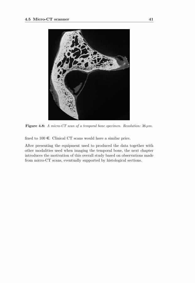
4.5 Micro-CT scanner 41
Figure 4.8: A micro-CT scan of a temporal bone specimen. Resolution: 36µm.
fixed to 100 e. Clinical CT scans would have a similar price.
After presenting the equipment used to produced the data together withother modalities used when imaging the temporal bone, the next chapterintroduces the motivation of this overall study based on observations madefrom micro-CT scans, eventually supported by histological sections.


5Observations from the data and
aims of the thesis
5.1 Introduction
In the litterature, the focus has been on the mastoid air cells as an overallsystem, [37, 46, 64, 79, 80, 88] and Paper I in this study. However, verylittle is known about the air cells when studied as a single entity. Inter-estingly, during this overall study, many questions were asked about theshape and size of a single air cell. Knowing the shape and size of an air cellalone is not so relevant, but to gain information about how much they varyin shape and size could provide information on the effect of a surroundingstructure locally. For instance, large air cells are thought to have very fewconstraints until some boundary conditions are large enough to stop theirevolution in size. Also, some large air cells may be the result of smallerair cells combining into one. It should be kept in mind that the mastoidbone is originally very flat, and possibly had similar characteristics as thecranial bone.
This chapter is an attempt to address these questions and proposes a pre-liminary study of how a mastoid air cell can be better characterised. Fourmain questions, that were most frequently asked, are stated in the remain-ing of this chapter with a brief answer to each of them. But before, thereis a need to define what is the midline of the mastoid air cell system, sinceit will be frequently used in this chapter.
5.2 Midline of the mastoid air cell system
The antrum, the transition between the tympanum and the mastoid aircell system, forms a major part of the midline. However, due to the varia-tion of the mastoid air cell system from one bone to another, the midline

44Chapter 5. Observations from the data and aims of the thesis
might be defined as a combination of the antrum along with the centralmastoid air cells directly protruding from the antrum, also known as cen-tral cells. Therefore, the notion of midline remains a relative geometricalnotion rather than just the antrum itself. How far the midline extends ver-tically towards the apex of the mastoid bone is also relative to the overallpneumatization of the bone under study. Now that the midline is defined,the questions are stated and a brief answer is proposed.
5.3 What is a mastoid air cell in terms of shape?
A cell, from the latin word cell meaning small room is used in multipleways in the British Dictionary as a small simple room commonly foundin a jail, convent, or in a monastery. A cell is also defined as a smallcompartment, found for instance in complex structures such as isolatingmaterials or honeycomb. In the field of biology, the word cell is also usedto either define the basic structural and functional unit of living organismsor any small cavity. This last definition is the one used throughout thisoverall study.
Figure 5.1: Surface rendering of a complete MACS together with the airspacesforming the tympanum. Source: [16].
As already introduced in Chapter 3, A. Allam followed by M. Tos classifiedthe air cells within the mastoid bone either based on their location or onanatomical structures in the vicinity, [3, 85]. However, a mastoid air cellcould also be classified based on its location in relation to the midline ofthe MACS: a terminal air cell or an intermediate air cell. A terminal aircould be defined as an air cell from which there is no more projection from.On the opposite, an intermediate air cell has the extra feature of extendingto another air cell(s); eventually to a terminal air cell. Terminal air cells

5.3 What is a mastoid air cell in terms of shape? 45
are easily observable at the outskirt of a rendered complete mastoid aircell system, see Fig. 5.1. To ease the reader’s understanding, a surfacerendering of the air cell system shown in Fig. 5.1 can be interpreted asa resin cast used to reveal their shape without the bone in which the aircells are carved into. It should be kept in mind that some terminal air cellsare also present halfway between the outskirt and the midline. Fig. 5.2illustrates the distinction between the terminal and intermediate air cells.
Figure 5.2: Distinction between terminal and intermediate air cell.
Communicating air cells may also be on a single branch, as represented inFig. 5.3 in a very simplistic manner.
Figure 5.3: Drawing of a simplistic isolated branch with a communicating air cellat its centre, and a terminal cell to the left separated by a conduitforming a necking.
From Figs. 5.2 and 5.3, another term is also introduced: conduits. Fromobservations on micro-CT scans of temporal bone specimens, a conduit isrepresented as a tubular structure that connects two air cells with eachother, whether of communicating type or of terminal type. Their lengthmay vary quite a lot; from very short where the two air cells are almostin contact with each others, to very long with a fairly constant diameteralong its main axis in most cases. In the presence of very short conduits,the word necking could also be used due to the large variation of diameter

46Chapter 5. Observations from the data and aims of the thesis
along its main axis. The word pore is also frequently used in other fields,such as stereology or in biology, but to keep the description simple, onlythe name conduit is used. Another, and more challenging, type of cells arethe finger-like type of cells. Though normally seen vertical, Fig. 5.4 givesan idea of how they look like.
Figure 5.4: Finger-like elongated type of air cells normally observed as vertical inthe mastoid, but represented horizontal for more practical purposes.
To illustrate how these structures appear in real cases, Fig.5.5 provides twodifferent views of an exposed mastoid process from a micro-CT scan usingvolume rendering.
Figure 5.5: Complexity of the mastoid air cell shapes revealed from a lateral view(left) and posterior view (right) of the same temporal bone using vol-ume rendering and clipped so as to exposed its internal part. Legend:(red arrows) finger-like elongated air cells, (yellow arrows) short con-duits, (blue arrows) necking forming pores between two cells, (greenstars) terminal cells in the more medial part of the MACS.

5.4 What is the size of an air cell? 47
5.4 What is the size of an air cell?
Park et al. [64], followed by many other other research teams, provideda framework on how to assess the surface area and volume of the overallmastoid air cell system, while using image processing on a stack of CTimages, [37, 46, 64, 79, 80, 88]. The estimates of surface area and volumefor a single mastoid air cell, though, remain unknown. When observinga surface rendering of the complete mastoid air cell system, as shown inFig. 5.1, the size of a singular air cell appears to vary considerably. Onedownside of such full representation is that, it does not allow visualizationof the more medial, i.e. more internal, cells and information on how theycommunicate with the midline. As explained in [13], clipping planes can beused to partially hide some of the rendered data in order to see the moreinternal parts of the air cell system.
Unfortunately, the complexity of the air cell system is so high that even us-ing clipping planes for visualization, it does not allow a clear understandingon how the air cell system is structured. It is although possible to clip mostof the air cell system and only preserve a small fraction to be rendered andstudy how air cells are locally connected to each others and eventually tothe midline. However, the connectivity with the remaining structure is notvisible and may lead to interpretation errors. Also, it is possible to performsuch a study by carefully studying a limited block of data at a time, andbuild a final three dimensional map, but besides the fact that it would takea tremendous amount of time to go through the overall volume, a lot oferrors may accumulate along the way.
From the new nominations given in the previous question, the originalquestion of what is the possible size of an air cell is changed to what is thesize of these structures, or more exactly how large these air cells are locally.When taking into consideration the fact that the air cells might be related tosurrounding structures, it is also considered relevant to investigate whetherthe variation in size of these structures is related to the regions over a fulltemporal bone as defined by [3, 85].
5.5 Air-mucosa versus mucosa-bone surface area
A striking but not surprising observation is the difference between the sur-face area of the interface air-to-mucosa interface that is much smaller thanthe corresponding surface area of the mucosa-to-bone interface. A typicalrepresentation from a histological section is illustrated in Fig. 5.6. Themucosa appears thinner in some places while thicker in more complex lo-

48Chapter 5. Observations from the data and aims of the thesis
cations. This local non-uniform thickness is possibly due to blood vessels,which participate in the gas exchange and therefore regulate the pressurelocally.
Figure 5.6: Nonuniform covering of the mucosa along the mastoid air cell walls.Source: Temporal Bone Histology Lab, Otorhinolaryngology, Uni-versity Zurich (permission granted by Prof. Dr. Med. AlexanderHuber).
A second but less obvious reason is the local thickening of the mucosa re-sulting from the remnants of a previous inflammation as detailed in Section3.8. Extensive cold is quite common and therefore it is very common toobserve these thickened mucosa from place to place. Therefore, there willbe a distinction between the surface area formed by the walls of the mastoidair cells, representing the interface bone-mucosa, and the more functionalsurface area defined by the interface mucosa-air.
Ideally, estimating the surface area from the air-to-mucosa interface wouldbe preferred. However, on micro-CT scans, the mucosa is too thin andbarely visible even for the highest scan resolution obtained in this overallstudy, i.e. 32µm. Estimation of the mucosa thickness was estimated byMatanda et al. [58] distances were 32µm ± 1.26 (mean ± σ) in the normalmucosa. As a side note, it is believed that even for locally enlarged mucosa,the distance between air to blood, an important factor for gas exchange,is kept constant and therefore this differentiation is not considered criticalin this study. Also, the thickness of inflamed mucosa was reported to22.32µm ± 0.59 (mean ± σ) but does not reflect the swollen epitheliallining due to the fact that it does not not impact the gas exchange fromair to blood. However, from a surface area point of view, the surface areaof the air-to-mucosa interface is certainly smaller than the surface areaestimated from mucosa-to-bone interface. As previously stated in Sec. 3.8,the mucosa can swell up to 80 times its original thickness.

5.6 Discovery of micro-channels 49
5.6 Discovery of micro-channels
Another observation is the discovery of numerous micro-channels found atthe cortex of the mastoid bone between the exterior and the lateral aircells, but also present between the air cells. These micro-channels havenot been described in previous literature. These micro-channels are likelyto represent a separate blood supply for the mastoid mucosa, and haveimportant implications for further understanding the middle ear physiologyincluding its pressure regulation and gas exchange.
Figure 5.7: Volume rendering of a temporal bone specimen with a special transferfunction, in order to reveal the micro-channels running in the bonebetween the mastoid air cells and outer layer of the bone. Clippingplanes were used to expose the internal parts of the bone. Both theuse of special transfer function and clipping planes are detailed inSec. 6.4.
To resume this section, the advantage of having at disposal micro-CT scansof complete mastoid air cell systems from several temporal bone specimens,and to compare the results from previous studies where conventional CTscanning was used is considered a high priority since more and more ENTdepartments perform such pneumatization studies involving surface areaand volume estimation. Performing a similar study using micro-CT scans,which is an uncommon procedure if not unique, may provide useful infor-mation for the rest of the community. The discovery of micro-channels,

50Chapter 5. Observations from the data and aims of the thesis
though not related to the size of the air cells, needs further investigationand is also considered a high priority in terms of new knowledge to bringto the field. Investigation of the shape of the mastoid air cells as singularentities is also an important topic, but belongs more to basic science interms of its use in the field. Also, studying the shape of singular air cells inorder to obtain a size distribution over a complete mastoid bone requiresmore tools from different fields. The next section provides a timeline onthe research has been carried out during the overall study.
5.7 Aims of the thesis
From the previous sections, the aims of this overall PhD study is twofolds:(1) Geometrical aspects of the mastoid air cell system related to pneuma-tization of the mastoid, (2) Interpretation and geometrical description ofthe discovered micro-channels penetrating the mastoid process. For eachtopic, a set of aims are defined and presented in the following.
Geometrical aspects of the mastoid air cell system
Aim 1. Determination of the surface area and the volume of the mastoidair cell system from X-ray micro-CT scans is necessary for estimating thepneumatization of the mastoid. The goal is to investigate whether scan-ning ex-vivo temporal bone specimens using X-ray micro-CT allows thedetection of a broader range of mastoid air cells in terms of size, especiallytowards air cells of smaller size, thus affecting the estimated surface areaand volume measures reported in previous literature.
Aim 2. Reducing the complexity of the mastoid air cell system represen-tation. Because the mastoid air cell system is very complex structure-wise,its binary representation remains complex in shape. It is believed that byreducing the complexity of the binary representation, while respecting themastoid air cell system topology, analysis beyond the estimation of the sur-face area and volume such as a 3D shape analysis is possible.
Aim 3. Investigate in a simplistic manner how inflammation of the mu-cosa lining mastoid air cells could impact the level of pneumatization ofthe mastoid through a 3D shape analysis. From the previous chapters, un-der inflammation, the mucosa lining the mastoid air cell might expand toa level where some air cells will be clotted. Depending on how large themastoid air cell system is locally, part of the air cell system may becometemporally or permanently dysfunctional. Measurements on the local size

5.7 Aims of the thesis 51
of the mastoid air cell system is therefore relevant to have.
Aim 4. Investigate whether the mastoid air cells do form groups or regionsas described by A. Allam and M. Tos. As described in the previous chap-ters, from observation of exposed mastoids, the mastoid air cells have beengrouped based on their location or according to neighbouring structure suchas the sigmoid sinus. However, there has not been any systematic way ofconfirming or rejecting this classification. A tool is therefore necessary toinvestigate this question.
Interpretation and geometrical description of the discoveredmicro-channels
Aim 5. Interpretation of micro-channels in the cortex of the mastoid pro-cess. Though already presented as an observation in the previous sectiondue to the high relevance, a more in depth description both in terms oftheir shape and their possible physiological role is needed.
Aim 6. Investigate the geometrical properties of the micro-channels. Dis-covery of a new anatomical structure such as the micro-channels penetrat-ing the bone of the mastoid process always leads to questions relating totheir geometry. Investigating their geometrical properties is therefore im-portant and further helps gaining knowledge about their potential role andpossible connection with surrounding structures.
Aim 7. Enhance the representation of micro-channels to get a better defi-nition of their course and connectivity. From the previous chapter, thoughthe X-ray micro-CT provides high resolutions scans, the resolution imposedby scanning the complete mastoid air cell system, together with artefactscommonly found using this technology, corrupt micro-channels of smallersizes. Incomplete representation of the micro-channels can lead to misinter-pretation of their connectivity and their implicit role from a physiologicalpoint of view. Enhancement of their course is therefore needed for futureanalysis.
In the following two chapters, the most relevant image processing toolsneeded to fulfil these aims are presented. In Chapter 6, image processingtools commonly used in the field of ENT are introduced. Then followsthe description of more advanced image processing tools used at severaloccasions in this study. An extra section is dedicated to volume rendering,clipping planes, and special masking. In Chapter 7, tools that do not belongto image processing but relate to 3D shape analysis are introduced.


6Image Processing
6.1 Introduction
This chapter provides a theoretical background of image processing, frombasic tools to more advanced ones. Common image processing tools of-ten encountered in clinical studies are resumed first. The reader can finda broader coverage in the literature such as in [25, 38]. More advancedmethods are then presented, and form the main framework for this overallstudy. A section about volume rendering is also included in this chapter,since it relates to visualization of results from image processing along withoriginal data.
6.1.1 Segmentation by thresholding
This section only deals with the type of segmentation used in this fieldof hearing research. Many other segmentation methods exist, such as thelocal adaptive threshold, but their description is beyond the scope of thisthesis and are seldomly used in the clinical field [91, 93]. The most commontechnique used in this field to isolate a structure from the rest of the datais called binary thresholding, which is applied in the following manner.Every pixel whose value is above a certain threshold, or within a certainrange of values, is interpreted as foreground value, usually set to 1, while allremaining pixels are considered as background, respectively set to 0. Fig.6.1 shows an example of an image segmented at different thresholds. In thisexample, the airspaces pixels below the threshold are segmented out andrepresented as white in the binary mask. As can be observed, the higherthe threshold the more structures are segmented along, including the bonemarrow in the trabecular spaces when the threshold is above 60.

54 Chapter 6. Image Processing
Figure 6.1: Binary segmentation of the airspace in the mastoid bone using differ-ent threshold values (40, 60, 80, 100, 120) compared to the originaldata (top left).
Also, it can be noticed that some of the segmented structures are attachedto each others, while they are not supposed to. This arises when the thresh-old is close to the bone range of grayscale values, and where the segmen-tation classifies some pixels belonging to bone as foreground (air) and notas background (bone). This type of error is illustrated in the simple repre-sentation shown in Fig. 6.2.
At the boundary of a structure, the CT intensity values change from thelevel of one tissue to that of another tissue. However, this change is gradualrather than abrupt, giving a blurred boundary interface. The interface, inperfect condition, is measured exactly halfway between the two CT num-ber levels, known as half maximum height, or HMH, representing the meanvalue of the two CT levels from both sides of the transition. Binary seg-mentation does not use any a-priori knowledge of the underlying structuresto be segmented. Therefore, all pixels or voxels above a certain value fromdifferent structures will be segmented at the same time, forming differentcomponents either connected or disconnected.

6.1 Introduction 55
Figure 6.2: Left: single structure, middle: two structures far apart leading tothe segmentation of the two structures, right: the structures are tooclose, which leads to a single object in the segmentation result. Notethat the pixels with a value below the threshold are set to white.
Because segmentation using the binary thresholding technique does notcontain information of the structure to keep, a manual selection of thatstructure needs to be done, see Fig. 6.3 to the right. The only require-ment is to make sure that the structure is disconnected from all segmentedstructures. The selection was performed using a region growing tool, byfirst placing a seed in the structure of interest, and letting the algorithmsegment all voxels belonging to the structure [36].
Figure 6.3: Selection of a region of interest (right) from the binary segmentation(middle) of the original data (left).
The result of the binary segmentation is often postprocessed using differentmorphological operations, which are described in the following section.
6.1.2 Morphology on binary images
Results from a binary segmentation can lead to misdetected or over-segmentedregions, while the remaining parts appear acceptable. One solution to cir-cumvent these issues is through the use of morphological operations. Fourmorphological operators are commonly used: dilation, erosion, opening,
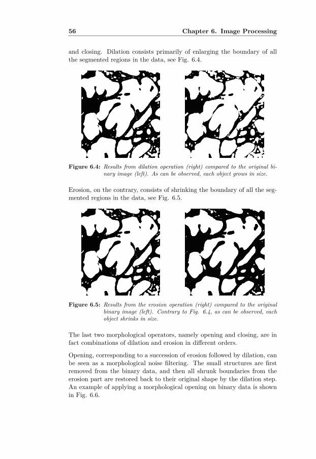
56 Chapter 6. Image Processing
and closing. Dilation consists primarily of enlarging the boundary of allthe segmented regions in the data, see Fig. 6.4.
Figure 6.4: Results from dilation operation (right) compared to the original bi-nary image (left). As can be observed, each object grows in size.
Erosion, on the contrary, consists of shrinking the boundary of all the seg-mented regions in the data, see Fig. 6.5.
Figure 6.5: Results from the erosion operation (right) compared to the originalbinary image (left). Contrary to Fig. 6.4, as can be observed, eachobject shrinks in size.
The last two morphological operators, namely opening and closing, are infact combinations of dilation and erosion in different orders.
Opening, corresponding to a succession of erosion followed by dilation, canbe seen as a morphological noise filtering. The small structures are firstremoved from the binary data, and then all shrunk boundaries from theerosion part are restored back to their original shape by the dilation step.An example of applying a morphological opening on binary data is shownin Fig. 6.6.

6.1 Introduction 57
Figure 6.6: The results from an opening operation (right) compared to the orig-inal binary image (left). Note that many small structures have dis-appeared.
Closing is, on the other hand, a succession of dilation and erosion. Whileopening removes noise in the binary data, closing can be interpreted asa filling small cavities present inside a binary structure. An example ofapplying a closing operation on a binary image is given in Fig. 6.7.
Figure 6.7: The result of a closing operation (right) compared to the originalbinary image (left), see the gray squares where merging occurred.
Despite a simple implementation and its usefulness for very simple shapes,such as a cube or a sphere in 3D, results from morphological operations arevery often unsatisfactory for natural images (i.e. medical images).
In some cases, even after a single pass of dilation or closing, some unwantedholes reside in the segmented object. A hole can be defined as a region ofpixels only having a background value (0), surrounded by a border of pixelswith foreground value (1). The algorithm, in that case, iteratively changesthe connected background pixels to foreground pixels and stops when the

58 Chapter 6. Image Processing
boundaries defining the hole of the segmented object are filled, see Fig. 6.8.
Figure 6.8: A (top left): binary segmentation of the bone, B (top right): re-sults from the hole filling where some holes were not processed dueto incomplete borders (sides of the image), C (bottom left): Modifiedversion of A with the left, top, and right sides of the image coveredwith a foreground value line. D (bottom right): successful filling ofthe holes in the bone.
The cavities present in the bone in Fig. 6.8(A), when fully surrounded byforeground value, are fully covered with foreground value, see Fig. 6.8(B).However, it can be noticed that some cavities were not filled due to theboundary not fully surrounding the cavity. To illustrate this problem, ver-tical and horizontal lines were added to the side of the image where bone ispresent, see Fig. 6.8(A). This step ensures that all cavities would be fullybe surrounded by a boundary, see Fig. 6.8(C). Only the lower right partof the image was not covered with a foreground line. When applying thehole filling algorithm on Fig. 6.8(C), all cavities inside the bone are then

6.1 Introduction 59
successively fully filled, see Fig. 6.8(D).
Such a technique can further help to extract a structure, such as the bone,with all its content. However, when looking at the binary results, it isalmost impossible to know what lies under the voxels added during themorphological step(s) being used. A possible way to verify what informa-tion lies under these added pixels/voxels is to reassign the original dataover the binary data, as explained in the following subsection.
6.1.3 Masking original data over a binary segmentation
A possible way to recover the original information from a binary segmen-tation, is to simply multiply the binary data by the original data, see Fig.6.9. All pixels or voxels that have a zero label will remain 0, while all theother pixels or voxels that are of label 1 from the binary image data willrecover the original grayscale value.
Figure 6.9: Reapplying the original grayscale data on the binary data (right), bymultiplying the binary segmentation (middle) with the original data(left).
In an image processing pipeline for visualization, such a method could bebe relevant. However, when used as an intermediate step, masking froma binary mask may introduce sharp edges on the side of the segmentedstructures and can further lead to additional errors, and can worsen theresults further when drawing statistics from such operations.
It may sometimes become a challenge to fix problems either related tothe original image itself, or resulting from one image processing operation.Eventually, it may become impossible to know where the problem comesfrom. For instance, changing the threshold in the binary segmentation mayresult in using an iteration of morphological operators, in order to allow thehole filling to work appropriately. Another example arises when seeking thetrue boundary of a bone. The CT level corresponding to the half maximumheight should be measured locally. This is the reason why it is difficult to

60 Chapter 6. Image Processing
decide a global threshold to the overall image.
Global thresholding techniques, such as the one introduced by Otsu ([69])which is commonly used in clinical research, are very fast and generallyproduce good results for the sole purpose of visualization. However, whenthe segmentation is aimed at measuring some metrics accurately, globalthresholding will not be adequate. Local thresholding techniques estimatea different threshold for each pixel, using the grayscale information from theneighbouring pixels. However, local thresholding is rarely used in clinicalresearch, possibly due the need for replicability of their study in relation toothers or simply by not knowing its existence.
Also, an early stage segmentation discards a lot of information from theoriginal data that could be used in further processing. A good practiceis to perform a segmentation at the very last stage, where all informationfrom the data needed for the study have been taken into account.
As the mastoid air cell system is now isolated from all other structures inthe data, metrics such as surface area and volume can be estimated, asexplained in the following.
6.1.4 Measuring surface area and volume
Estimating the volume from 3D data is fairly straightforward. It is usuallydone through counting the number of voxels belonging to the structure,and multiplying this number by the voxel size. Voxels containing a mixtureof several tissue types within the same voxel, also known as the partialvolume effect, also need to be included since they contain a portion of air inthem. A solution is to reapply the original data on the binary segmentationthrough the masking operation, as explained previously. The result fromthe masked data is then inverted, so that it can be used as a percentagerepresentation of the content of air in the mastoid air cells.
When the voxels only consist of air (white), it will represent 100% of thevoxel volume. Additionally, when a voxel contains a mixture of tissues, thevolume of air in that voxel will provide a percentage proportional to theamount of air in it. As an example, if a voxel contains 50 % of both air andsoft tissue, the volume of air will be 0.5 of the voxel volume correspondingto air. This method produces a slightly more accurate volume estimate,compared to directly using the binary segmentation. It should be notedthat the presence of noise, as in in Fig. 6.9, can also have an influenceon the volume measurement for such a technique, but is still believed tobe a more accurate measure than estimating the volume from the binarysegmentation.

6.1 Introduction 61
Figure 6.10: Surface mesh of a complete mastoid air cell system generated froma regular clinical CT scan (512 × 512 pixels with a slice thicknessof 0.625mm).
The surface area, however, is more challenging to estimate. One technique,commonly used in many medical image processing applications, is to fit atriangular mesh from a binary segmentation [53], from which it is possible tomeasure the surface area. For each triangle composing the mesh, the area iscomputed and the sum of each triangle area is then accumulated, to give thetotal surface area over the whole mesh. Fig. 6.10 provides an illustrationof such a triangular mesh, from which the surface area can be estimated.Using such a triangular mesh, fitted to a binary segmented volume, dependsheavily on the resolution of the original data. If the resolution is too low,a triangular mesh will be composed of relatively large triangles, and willtherefore give a rough estimate of the surface area. When the original datais of much higher resolution, the triangles composing the mesh will be muchsmaller, thereby giving a much more accurate estimate of the surface area.
All the mentioned methods are based on the grayscale values of the origi-nal data. As introduced earlier, noise will corrupt the grayscale intensitiesand will inevitably lead to using different "tricks" to circumvent some ofthe encountered issues. Moreover, it may be difficult to define a specificorder when using different image processing tools. Nonetheless, it is of-ten necessary to assess the results from one step, go back to a previousstep, re-tune the parameters for that step, and move on to the followingsteps, leading to a hit-or-miss type of global method. While some meth-ods can be used globally for the whole image, some require local adaptivity.

62 Chapter 6. Image Processing
Also, it can be noted that this line of thinking leads to segmenting the struc-ture of interest in order to extract information from it. Another strategyis to define the conditions for the structures of interest to be investigated,and use such a-priori information in order to extract these structures fromthe original input data.
6.2 More advanced image processing
In this section, a different line of thinking is presented. It relates to ex-tracting all relevant a-priori information about the structure of interest, andthen use this information to guide the algorithm to detect these structuresof interest. Before defining the conditions to find such a-priori information,several topics need to be introduced to understand this line of thinking.For humans, as for many other species, vision is a very important part ofour sensory system. Detecting a special object of interest in the surround-ing involves different sources of information such as for instance colours,patterns, and shapes.
In fact, an object is mostly characterized by its size and its edges, whetherbeing sharp or smooth. Lines are also important in the vision system, sincethey allow us to delineate between different structures or objects. Usingsuch information is therefore essential when looking for a specific structurein a 2D image or 3D volume.
Figure 6.11: Examples of lines and edges.
Even if an object of interest globally has a very complex structure, it canlocally be represented with very simple structures such as lines and edges,all with different orientations, see Fig. 6.11. A real case is shown in Fig.6.12.
Such transitions, whether a line or an edge, can be seen as simple signalsin 1D. One approach is to geenrate a one-dimensional template for a lineand for an edge, rotate these templates in several directions (2D or 3D),and detect them in the original 2D image or 3D volume (using convolution).

6.2 More advanced image processing 63
Figure 6.12: Lines and edges in different regions of an image.
Relevant tools from digital signal processing can be used when building suchfilters [45]. As will be explained in the following of the thesis, informationabout the frequency domain along with the spatial domain is needed. Infact any signal, such as a complete image, can be decomposed in terms ofsinusoids with different frequencies. For instance, if a profile is taken alonga single image from a data scan, the grayscale intensity profile along thatline can be extracted, see Fig. 6.13. It should be noted that a line in 2Dcorresponds to a sheet or a surface in 3D.
Figure 6.13: Grayscale intensity profile (right) extracted from the white line over-laid on the original image (left).
According to Fourier theory, the signal describing the profile can be decom-posed into sinusoids each having a unique frequency, see Fig. 6.14. When

64 Chapter 6. Image Processing
combining all these sinusoids with respective frequencies, it is possible toreconstruct the original profile shown in Fig. 6.14. In this example, thereconstruction from three different set of frequencies are shown. It can beobserved that the reconstructed profile in the lower graph is very similarto the intensity profile shown to the right in Fig. 6.13.
Figure 6.14: Reconstruction of the intensity profile given in Fig. 6.13 from threedifferent sets of sinusoids.
The operation of representing this intensity profile into sinusoids of differ-ent frequency was performed through a so-called Fourier transform. TheFourier transform plays a central role in signal and image processing, andis used when defining the template for line and edge detection in this study.
In the following section, all elements related to the design of the line andedge filters are briefly introduced focusing more on the philosophy ratherthan on the mathematical aspect, though some mathematical expressionswill be given. A more complete introduction is given in [26].
6.2.1 Filter design
As introduced earlier, the edges and lines defining the structures can bedecomposed in terms of sines and cosines. To pick up sine and cosineinformation from a natural signal, a solution is to create a filter which is onlysensitive to a certain wavelength or range of frequencies. For illustrativepurposes, only a single frequency is shown in the following figures. Before

6.2 More advanced image processing 65
digging into the filter design, the Fourier transform of both the cosine andsine needs to be resumed first. For the cosine, defined as f(t) = cos(ωt)with ω = 2πf for a 1D signal in the spatial domain, the Fourier transformbecomes
F (u) =∫ ∞−∞
f(t)e−i 2πutdt
=∫ ∞−∞
cos(ωt)e−i 2πutdt
=∫ ∞−∞
cos(ωt)[cos(−2πut) + i sin(−2πut)]dt
=∫ ∞−∞
cos(ωt) cos(−2πut)dt+ i
∫ ∞−∞
cos(ωt) sin(−2πut)]dt
=∫ ∞−∞
cos(ωt) cos(−2πut)dt︸ ︷︷ ︸6= 0 when u = ±ω
− i∫ ∞−∞
cos(ωt) sin(2πut)]dt︸ ︷︷ ︸= 0 for all u.
= 12[δ(u+ w) + δ(u− w)]. (6.1)
The Fourier transform of a cosine is illustrated in Fig. 6.15, where twoimpulse responses are located at −ω and +ω.
Figure 6.15: Fourier transform of a cosine.
Similarly for the sine wave, defined as f(t) = sin(ωt) with ω = 2πf in 1Din the spatial domain, the Fourier transform becomes:
F (u) = 12 i [δ(u + ω)− δ(u − ω)]. (6.2)
As can observed, the Fourier transform of the sine is imaginary, see Fig.6.16.

66 Chapter 6. Image Processing
Figure 6.16: Fourier transform of a sine.
Fig. 6.17 shows side by side, using three axes, the Fourier transform ofcos(wt) and sin(wt). The Fourier transform of the cosine lies along theplane formed by the real axis and the frequency axis. The Fourier transformof the sine lies on the plane formed by the imaginary axis and the frequencyaxis, normal to the real plane.
Figure 6.17: Fourier transform of cosine located along the real plane (left), andFourier transform of the sine is located along the imaginary plane,normal to the real plane (right).
To avoid involving complex notation, a possible solution is to perform theFourier transform of i sin(ωt) instead of sin(ωt), leading to a rotation of theFourier transform of the sine along the real plane instead of the imaginaryplane, see Fig. 6.18

6.2 More advanced image processing 67
Figure 6.18: Fourier transform of cosine and the complex sine (isin) are bothlying along the real plane.
Obviously, since the Fourier transform of a cosine and a sine each produceonly a set of impulses for both ω and −ω whether positive or negative,using such an impulse response to design a filter would make no sense,since their inverse Fourier transform would have an infinite support in thespatial domain. A filter by definition needs to be local, in order to extractlocal information from an image. To achieve locality, by forming a pulsetrain around a centre frequency and adding the contribution of each impulsethen produces a filter that becomes more and more local. As an example,observe a cosine and a sine for 5 different frequencies, see Fig. 6.19.
Figure 6.19: 5 cosines (left) and sines (right) with the same respective frequen-cies, represented both in the spatial domain and in the frequencydomain. Only one period is represented for clarity purpose, buteach impulse in the frequency domain represents a infinite long co-sine or sine of the specified frequency.
When adding cosines with different frequencies together, a major signal

68 Chapter 6. Image Processing
component appears at the centre with some ripples on both sides, see Fig.6.20 (left column). The same applies for the sine components added to-gether, Fig. 6.20 (right column).
Figure 6.20: Summation over 5 frequencies in the spatial domain for both thecosine (left) and sine (right), and representation of the impulsesthat were used during the summation.
The quest of localization for the filter is then to suppress the ripples onboth sides of the signal, while keeping the major component. To give moreemphasis on the main lobes at the centre of the signals in Fig. 6.20, whileattempting to discard the ripples, a weighting window or function can beapplied to the impulses used during the summation. In Fig. 6.21, twodifferent types of weighting are applied. A first weighting function is madelinear corresponding to a pyramid, with for instance a weight of 0.1 forthe outmost frequency in relation to ω (respectively −ω), a weight of 0.5is given to the innermost impulse, while the middle impulse, ω or −ω, isgiven a weight of 1. In the second part a non-linear weighting function(Gaussian) is used instead of a linear one, which for this example has theweights: 0.2, 0.7, 1, 0.7, and 0.2 respectively.
The ripples are minimized by the nonlinear weighting function, making thefilter in the spatial domain very localized. Overlapping the resulting signalsfrom the non-linear weighting - i.e. cosine and sine - in the spatial domain,we can observe a good match in localization, see Fig. 6.22.

6.2 More advanced image processing 69
Figure 6.21: Linear and non-linear weighting functions applied to the impulsesbefore summation, making the signals in the spatial domain morelocalized.
Figure 6.22: Overlapping the results from the non-linear weighting of both thecosine (even) and sine (odd).
From Fig. 6.22, the left signal is even in relation to its centre and is definedin the real part as illustrated in Fig. 6.17 to the left. The second signal tothe left is odd in relation to its centre, and is defined in the imaginary partas illustrated in Fig. 6.17 to the right. If the even part is denoted fe(x) andthe odd part denoted fo(x), we can see that fo(x) is the Hilbert transformof fe(x). This property leads to the notion of quadrature, where these twocomponents form a complex pair in the spatial domain. The real part isdefined as a line filter and the imaginary part is defined as an edge filter.The cosine can be seen as a line detector, and the weighted sine can be seenas an edge detector. Together, these two filters form a quadrature filter.When convolving the quadrature filter over an image, when a line structureis met, the response of the filter will be dominant in the real part, whilewhen the filter encounters an edge, it will produce an imaginary response.It is possible to map the type of structure encountered in the image, usingthe so-called local phase and local amplitude or magnitude [43]. The local

70 Chapter 6. Image Processing
phase is defined as
θ(x) = arctan{ fo(x) ∗ f(x)
fe(x) ∗ f(x)
}= Im(q)
Re(q) (6.3)
where ∗ denotes the convolution operation. The local magnitude is ex-pressed as
A(x) =√
[fe(x) ∗ f(x)]2 + [fo(x) ∗ f(x)]2. (6.4)
The local phase can be mapped on a complex plane where θ represents theangle and A represents the magnitude of the vector, illustrated in Fig. 6.23.
Figure 6.23: Coding of the local phase.
The advantage of using the local phase from quadrature filters is the factthat it is contrast independent. While gradient-based type of filters canmost of the time only detect edges formed by rapid transitions betweentwo distinct regions of different intensities, the gradient-based filters willvery often fail in detecting smooth edges or edges having low contrast [47].In the case of a line, hardly detectable using common gradient-based filters,a quadrature filter will provide the same local phase for a strong line as fora weak line. A strong magnitude provides a high confidence in the detectedstructure type. In locations where the magnitude is close to zero, meaninglow confidence, the local phase mainly represents noise. In Fig. 6.23, theargument of the local phase is kept constant to a maximum on the unitcircle.
The quadrature filter used in this work is presented in the next section.
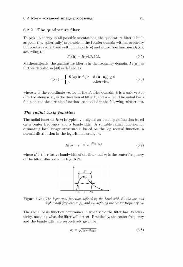
6.2 More advanced image processing 71
6.2.2 The quadrature filter
To pick up energy in all possible orientations, the quadrature filter is builtas polar (i.e. spherically) separable in the Fourier domain with an arbitrarybut positive radial bandwidth functionR(ρ) and a direction functionDk(u),according to
Fk(u) = R(ρ)Dk(u). (6.5)
Mathematically, the quadrature filter is in the frequency domain, Fk(u), asfurther detailed in [43] is defined as
Fk(u) ={R(ρ)(uT nk)2 if (u · nk) ≥ 00 otherwise, (6.6)
where u is the coordinate vector in the Fourier domain, u is a unit vectordirected along u, nk is the direction of filter k, and ρ = |u|. The radial basisfunction and the direction function are detailed in the following subsections.
The radial basis functionThe radial function R(ρ) is typically designed as a bandpass function basedon a center frequency and a bandwidth. A suitable radial function forestimating local image structure is based on the log normal function, anormal distribution in the logarithmic scale, i.e.
R(ρ) = e−4
B2ln2ln2(ρ/ρ0) (6.7)
where B is the relative bandwidth of the filter and ρ0 is the center frequencyof the filter, illustrated in Fig. 6.24.
Figure 6.24: The lognormal function defined by the bandwidth B, the low andhigh cutoff frequencies ρL and ρH defining the center frequency ρ0.
The radial basis function determines in what scale the filter has its sensi-tivity, meaning what the filter will detect. Practically, the center frequencyand the bandwidth, are respectively given by:
ρ0 = √ρlow.ρhigh, (6.8)

72 Chapter 6. Image Processing
and
β =logn(ρhigh
ρlow)
logn2 (dB), (6.9)
with ρhigh and ρlow corresponding to the high and low frequency boundsdefining the bandwidth of the filter. The centre frequency corresponds toa wavelength (measured in pixels) of
λ0 = 2πρ0. (6.10)
The spatial size of the filter needs to be at least one wavelength, and inpractice 1.5 or even 2 wavelengths. Table tab:Chap6Table1 show the spatialsize for three different center frequencies.
centre frequency µ0 wavelength λ0 linewidth(λ0/2)π 2 pixels 1 pixelsπ/2 4 pixels 2 pixelsπ/4 8 pixels 4 pixels
Table 6.1: Correspondance between the centre frequency, the wavelength, and thewidth of the line to be detected.
The direction functionThe direction function, Dk(u), varies as cos2(φ), where φ is the angle be-tween u and the filter direction nk, given by
Dk(u) ={
(u · nk)2 if (u · nk) ≥ 00 otherwise. (6.11)
In 3D, it is common to use six quadrature filters along different directions,see [26] for further explanations about this specific choice. The six direc-tions are defined as
n1 = c (a 0 b)T ,n2 = c (−a 0 b)T ,n3 = c (b a 0)T ,n4 = c (b −a b)T ,n5 = c (0 b a)T ,n6 = c (0 b −a)T ,
(6.12)
with a = 2, b = 1 +√
5, and c = 1√10+2
√5.
The combination of the radial function and the angular function is sum-marized in Fig. 6.25. The radial function is by itself smooth, but to get

6.2 More advanced image processing 73
a smooth transition between the different quadratures, a cos2 function isused as a directional function.
Figure 6.25: Sketch of the radial and angular functions for different directionsk, with their respective smooth variations.
Without the cos2 weighting, the sharp transitions would result in undesiredeffects on the final output data. In 3D, a spherical shell with a thicknesscorresponding to the bandwidth of the radial function would be formed.A pseudo-representation of the radial function in 2D is given in Fig. 6.26,illustrating the lognormal function used as a radial function viewed fromabove.
Figure 6.26: Pseudo-representation of the lognormal radial function in 2D.
The magnitude of the quadrature filter output is computed as
qk = ‖ 12π
∫S(u)Fk(u) du‖, (6.13)
where S(u) is the Fourier transform of the original data set.

74 Chapter 6. Image Processing
Because both spatial and frequency domains are considered at the sametime, an operation called filter optimisation is needed [44, 45]. An exampleof the real and imaginary parts of an optimised quadrature filter is givenin Fig. 6.27, and the corresponding optimized quadrature filter in thefrequency domain is illustrated in Fig. 6.28.
Figure 6.27: Real and imaginary part of an optimized quadrature filter: left) realpart, b) imaginary part.
Figure 6.28: An optimized quadrature filter in the frequency domain.
For the local neighborhood of each visited voxel, the filter response providesa contribution from six directions. . The contribution of the filter responsefrom each direction of detected local structure needs to be stored, for eachvisited voxel in the volume. Such a contribution cannot be represented bya point or a vector alone. A structure to englobe the total information foreach voxel is therefore needed.
The need of storing the contribution from each direction for each voxelhas been encountered in many fields, where physical properties need tobe locally described. A mathematical field has emerged where tensors canrepresent all the information in each voxel. The notion of tensor should notto be confounded with the muscle type, such as the tensor tympani used todampen sounds generated while chewing. Derivation of the tensor analysisis briefly stated in the following section.

6.2 More advanced image processing 75
6.2.3 Tensor analysis
While a vector is defined as a list of values, and a matrix is defined as atable of values, the natural evolution of such taxonomy would be a list oftables or a table of lists. Therefore, tensors can be seen as a generalizationof matrix of N dimension. When considering more than one direction, suchas in the case of the quadrature filtering with the contribution from sixdifferent directions, a tensor is an adequate solution.
The next step in this study is to compute the structure tensor, which ineach voxel contains information about the local structure. The naming ofstructure tensor will be used during the rest of the thesis. The estimate ofthe structure tensor can now be constructed as
Test =6∑
k=1|qk|Mk, (6.14)
with |qk| being the magnitude of the quadrature filter output, and Mk isdefined as
α nknTk − β I (6.15)
where nk is the direction of quadrature filter k, I is the identity matrix, αis 5/4, and β is 1/4 in the 3D case, see [26] for more details on the choice ofα and β. Because the tensor matrix is symmetric, the tensor componentscan also be written as follows (for the 3D case):
T =
t11 t12 t13t12 t22 t23t13 t23 t33
(6.16)
The advantage of using a tensor resides in the possibility of extractingthe eigenvalues (λi) and eigenvectors (ei) from the local structures. Theeigenvalues and eigenvectors inform us about the energy distribution of thesignal in each voxel. The main reason of extracting the eigenvalues andeigenvectors is the possibility to visualize such information through the useof ellipsoids. Ellipsoids are defined with three axes, the eigenvectors, andthe magnitude defined along each axis determines the shape of the ellipsoidthrough the eigenvalues, see Fig. 6.29.
Specific combinations of eigenvalues can be defined to separate differenttypes of structures. Linear structures (also known as prolate or cigar-shaped structure), can be extracted when λ1 � λ2 ' λ3. λ1 is the dominantcomponent, while λ2 and λ3 are similar but much smaller in magnitudecompared to λ1, see Fig. 6.29(A). Linear structures are of type rank 2tensor.

76 Chapter 6. Image Processing
Figure 6.29: Ellipsoids defining: (A) the linear case with λ1 � λ2 ' λ3, (B) theplanar case where λ1 ' λ2 � λ3, and (C) the isotropic case whereλ1 ' λ2 ' λ3. Source: [15].
Planar structures (also known as oblate or disc-like) can be extracted whenλ1 ' λ2 � λ3. In this case, λ1 and λ2 are similar and much larger thanλ3. Therefore the two dominant components λ1 and λ2 form a plane witha slight protrusion along λ3, see Fig. 6.29(B). Planar structures are of typerank 1 tensor.
Isotropic structures (also known as spherical) can be extracted when λ1 'λ2 ' λ3. In that case, because all eigenvalues are equivalent, the ellip-soid becomes a sphere without any specific orientation and therefore calledisotropic, see Fig. 6.29(C). Isotropic structures are of type rank 3 tensor.
6.2.4 Extraction of planar, tubular, and isotropic structures
The eigenvalues from the structure tensor can be used to estimate theprobability of each visited neighborhood belonging to either a rank 1, arank 2, or a rank 3 tensor, defined by p1, p2, and p3, where
∑3k=1 pk = 1
which can be seen as probabilities [26]. The probabilities are calculated as
p1 = λ1 − λ2λ1
, p2 = λ2 − λ3λ1
, p3 = λ3λ1. (6.17)
The micro-channels, as any other natural structure, are however composedof a mixture of these three cases and a more general ideal structure tensorcan instead be represented by
T = p1T1 + p2T2 + p3T3 (6.18)
Examples of rank 1, rank 2, and rank 3 tensors are given in Fig. 6.30 forseveral elliptical cylinders, having different sizes and for different orienta-tions. The rank 1 tensor is displayed as blue (planar), the rank 2 tensor ismapped with the red colour (linear or tubular), while the rank 3 tensor is

6.2 More advanced image processing 77
rendered in green (isotropic). To better locate the structure tensors loca-tions in relation to the original data, the original data was rendered alongwith each presented case.
In Fig. 6.30(A), the original data is rendered semi-transparent. In Fig.6.30(B), the rank 2 tensor is rendered alone and overlaid on the originaldata. In Fig. 6.30(C), the rank 1 tensor is rendered alone and overlaid onthe original data. In Fig. 6.30(D), the rank 3 tensor is rendered alone andoverlaid on the original data. In Fig. 6.30(E), the rank 1 and 2 tensors arerendered together. In Fig. 6.30(F), the rank 1 and 3 tensors are renderedtogether and overlaid on the original data. In Fig. 6.30(G), the rank 2and rank 3 tensors are rendered together and overlaid over the originaldata. Fig. 6.30(H) shows the combination of all cases together, illustratingtheir complementarity. For the rank 2 tensor, the tubular structures are
Figure 6.30: Extraction of rank 1, rank 2, and rank 3 tensors on elliptical cylin-ders of different sizes placed with different orientations. (A) orig-inal data, (B) rank 2 tensor alone, (C) rank 1 tensor alone, (D)rank 3 tensor alone, (E) rank 1 and 2 tensors rendered together,(F) rank 1 and 3 tensors rendered together, (G) rank 2 and 3 ten-sors rendered together, and (H) rank 1, rank 2 and rank 3 tensorsrendered altogether.
effectively representing the edges of the cylinders along with the very thincylinder being represented by a rank 2 tensor on most of its path, exceptat its extremities where it shows rank 3 tensor information. Notice theappearance of the very thin cylinder displayed as semi-transparent in therank 1 tensor case alone, while there should not be any information for thisthin cylinder, see Fig. 6.30(C). In the sole presence of a rank 3 tensor, asshown in Fig. 6.30(D), or in the case of rank 1 tensor rendered togetherwith rank 3 tensor, as represented in Fig. 6.30(F), the results overlaid on

78 Chapter 6. Image Processing
the original data helps locating the isotropic information at the extremitiesof the very thin cylinder.
The respective p1, p2, and p3, along with their combinations p1 & p2 orp1 & p3, or p2 & p3 are illustrated in Fig. 6.31. Although the separate cases- p1 to the left, p2 at the middle and p3 to the right - alone on the toprow clearly indicate their respective contribution in terms of energy, theirrelation with each others is difficult to visualize. Combining two casesat a time gives a better understanding of how the structures are related.The lower right image indicates where the tubular structures are locatedin relation to the neighbouring planar structures. The middle low imageshows the isotropic part within the bone mostly prominent in the thick partof the bone, where the density changes very little in a small neighbourhood.The lower right image gives an indication of how the tubular structures mixwith the isotropic structures.
Figure 6.31: The three cases p1, p2, and p3 and their combination p1 & p2 orp1 & p3, or p2 & p3. p1 represents the planar part structures, p2represents the linear/tubular structures, p3 represents the isotropicconstribution.

6.3 Enhancement through adaptive filtering 79
The complete combination, i.e. p1, p2, and p3 altogether, is illustrated inFig. 6.32. The original data, to the left, is represented simultaneously,to allow a better understanding of the results from the structure tensor interms of p1, p2, and p3 to the right.
Figure 6.32: Combination of all cases p1, p2, and p3 (right) compared to theoriginal micro-CT data (left).
6.3 Enhancement through adaptive filtering
When carefully observing the results in Paper III, the very thin micro-channels are not fully represented along their path. The noise further cor-rupts their definition. A natural step is, therefore, to reduce the noiselevel as much as possible, while at the same time enhance the weak micro-channels by favouring the linear/tubular structure information from thelocal structure tensor analysis. This process is known as anisotropic adap-tive filtering and has previously been used in 2D, 3D, and even 4D [21,29, 55, 76]. Similar to [76], the enhanced data fa is an adaptive filteringdefined as
fa = flp +6∑
k=1wk fbp,k, (6.19)
where flp is a lowpass filtered version of the volume, wk being a set of scalarvalues, and fbp,k represent the filter response from different bandpass filterswith the same directions as the quadrature filters. The structure tensor

80 Chapter 6. Image Processing
given in Eq. 6.18 can be estimated as
Test =6∑
k=1‖qk‖(α nknTk − β I). (6.20)
To express the adaptive filter in terms of the local structure tensor, thescalar values wk can be estimated by projection of the local structure tensoronto a set of dual tensors Mk corresponding to (α nknTk − β I) in the righthand side of Eq.6.20, such that the enhanced volume is defined as
fa = flp +6∑
k=1〈T,Mk〉fbp,k. (6.21)
Enhancement can be performed using the local structure tensor, throughtensor processing via the building of a control tensor C. After smoothingthe components of Test using a small isotropic low-pass kernel, to preventrapid changes in the tensor field, a soft threshold of the norm of the low-passfiltered tensor is computed
T = γ(‖Tlp‖)‖Tlp‖
Tlp, (6.22)
where Tlp = hlp ∗ Test and γ is a smooth mapping corresponding to low-parametric sigmoid function defined for α ∈ [0, 1] as
γ(x, σ;α, β) = xβ
xα+β + σβ, (6.23)
The γ-function controls the amount of anisotropic high-pass filtering, al-lowing a bandwidth selectivity. Well defined structures are therefore rep-resented by a large norm while small fluctuations, such as noise, are rep-resented by a small norm. The σ parameter can be understood as anestimate of the noise in the data. The α parameter is typically in the rangeof [0, 0.5], and is used to accentuate weak structures that are right abovethe noise level. The parameter β sets the main slope of the γ-function inthe noise-signal transition [26].
Fig. 6.33 gives an overview of the γ-function where only σ varies in arange of [0, 1]. When σ = 0, all frequencies are taken into account, noiseincluded, while when σ = 1 only the low frequencies are preserved. The redcurve illustrates the setting used when enhancing the micro-channels withσ = 0.15, α = 0.07, and β = 8. Fig. 6.34 shows the effect of varying α inthe γ-function. Low values of α will often result in a high-pass filter slowlytending to 1 as x tends to 1. Higher values of α will produce a peak rightafter the main slope, and will gradually converge back to 1 as x tends to1. Fig. 6.35 gives an indication of how the slope of the γ-function behaveswhen only modifying the β parameter.

6.3 Enhancement through adaptive filtering 81
Figure 6.33: γ-function where only σ varies. A special case is shown with σ =0.15, α = 0.07, and β = 8 (red curve).
Figure 6.34: γ-function where only α varies. The red curve is a setting withσ = 0.15, α = 0.07, and β = 8, allowing a large range of frequenciesbut with no amplification in the selected bandwidth.
Figure 6.35: γ-function where only β varies. The red curve is a special settingwith σ = 0.145, α = 0.3, and β = 8, accepting a fairly large rangeof frequencies but with a substantial amplification in the high fre-quencies.

82 Chapter 6. Image Processing
The output of the γ-function corresponds to the largest eigenvalue, i.e. γ1,of the control tensor C. Therefore, choosing the parameters governing theγ-function will influence the bandwidth selection of the high-pass filter inthe enhancement scheme. All these parameters, σ, α, and β have an influ-ence on each others, and their settings heavily depend on the applicationand how much noise there is in the data being processed. Noisy data willgenerally imply a low σ. If the goal is to only enhance very small weakstructures in noisy data, α needs to be adjusted in consequent so as toonly enhance weak structures, while preserving larger structures as theyare. The fact that the structures are small, implies a high frequency repre-sentation as previously explained, and therefore α will have an impact onthe noise level amplification, since it will also amplify the noise level.
Therefore, σ and α should be chosen carefully in relation to each other.The slope of the γ also needs to be considered. To control the shape ofthe adaptive filter, i.e. the orientational variation in the high-pass regions,the ratio of the eigenvalues of the local structure tensor can be used andremapped using the µ-function such as
µ(x;α, β) =[ (x(1− α))β
(x(1− α))β + (α(1− x))β], (6.24)
where x = λnλn−1
. The parameter α is defined in the µ-function as the valueof λn
λn−1for which the µ-function is equal to 1
2 . A representation of α forthe µ-function is given in Fig. 6.36, where α is varying from [0, 1] and β iskept constant and equal to 8.
Figure 6.36: µ-function where only α varies, while β is kept constant. The redcurve is an example of a special setting with α = 0.3 and β = 8.
As for the β parameter, it defines the slope in the transition area in thesame manner as for β in the γ-function, see Eq. 6.23. A representation ofβ for the µ-function is given in Fig. 6.37 where β is varying from [1, 10]while α kept constant and equal to 0.3.

6.3 Enhancement through adaptive filtering 83
Figure 6.37: µ-function where only β varies, while α is kept constant. The redcurve is an example of a special setting with α = 0.3 and β = 8.
The resulting µn will correspond to the filter shape coefficients. The con-trol tensor can now be constructed based on its largest eigenvalue γ1 andthe filter shape coefficients. Reusing the eigensystem from the original lo-cal structure tensor ensures a preservation of the orientation estimation.Therefore, the control tensor can be written as
C = γ1[e1eT1 + µ2[e2eT2 + · · ·+ µN [eN eTN ] + · · · ]], (6.25)
where eTn are the eigenvectors of Tlp. Eq. 6.25 can then be rewritten as aweighted sum of outer products of Tlp as
C =3∑
n=1γkeneTn , (6.26)
leading to a modification of Eq. 6.21, such that
fa = flp +6∑
k=1〈C,Mk〉fbp,k. (6.27)
A high-pass amplification factor was further added to Eq. 6.27 to favourenhancement of solely linear or tubular structures by using the eigenvaluesfrom the structure tensor according to
fa = flp + ahp
6∑k=1〈C,Mk〉fbp,k , (6.28)
where ahp is defined as
ahp = ξ · ν1 λ1 + ν2 λ2 + ν3 λ3ν4 λ1 + ν5 λ2 + ν6 λ3
, (6.29)

84 Chapter 6. Image Processing
with ξ set to 1.7 in Paper IV along with ν =[3 1 −1 2 −1 1
]. The
enhanced data can be resumed as the sum of a low-pass filtered version ofthe original data, applied only once, with a linear combination of anisotropichigh-pass filters using the corresponding directions of the quadrature filter,and where the scalars wk are mapped by the control tensor.
Ienh = Ilp +6∑
k=1wk Ibp (6.30)
Examples of image enhancement using adaptive filtering are given in Figs.6.38, 6.39, 6.40, and 6.41.
Figure 6.38: Volume rendering of the enhanced data (right) versus the originaldata (left) of a partial bone specimen viewed from the medial side,with the antero-superior part of the tympanum at the top left andthe antrum seen as the dark region central to the sample.
In Fig. 6.38, a volume rendering of the enhanced data, seen partially, isplaced side by side with the original data, to be able to see the achievedenhancement. Fig. 6.39 gives a zoomed representation of Fig. 6.38, prin-cipally at the lower right region. While it is difficult to appreciate theenhancement achieved on Fig. 6.38, due to the sole enhancement of finestructures corresponding to about 4 to 8 pixels, Fig. 6.39 allows a betterdistinction of weak structures from the original data when compared to itsenhanced version.Interestingly, the enhancement further accentuates the notion of depth andtherefore 3D perception. In fact, the difference in depth perception relates,in this study, to a preservation of the transfer function based on the orig-inal data when observing the enhanced data. To optimize the comparisonbetween the enhanced and the original data, the transfer function shouldbe modified accordingly. Attempts to match the transfer function for boththe original and the enhanced data were made, but relates more to a hit-and-miss operation, and therefore a similar transfer function was used forboth datasets.

6.3 Enhancement through adaptive filtering 85
Figure 6.39: Zoomed version of Fig. 6.38 to better appreciate the details of theenhancement (right) compared to the original data (left).
Figure 6.40: Comparison of the enhanced (right) versus the original data (left),where the micro-channels are revealed while using a transfer func-tion similar to Fig. 6.44 (D).
To fully appreciate the benefit of enhancing the micro-channels, for whichthe quadrature filters are optimized, Fig. 6.40 shows a comparison betweenthe original data and the enhanced data. The micro-channels, visible to theright side of both the original and enhanced data, are more easily readablein terms of structure in the enhanced data than in the original data. Insome locations, in the original data, the micro-channels appear disruptedby noise. In the enhanced data, the combination of lowpass filtering thenoise in combination with amplifying weak structures clearly improve theirconnectivity.
Fig. 6.40 also reveals an important feature. Between the micro-channels,the noise appears more dense in some part than in others. If too dense, thenoise will not be completely removed but will result in more blurry regionsbetween the micro-channels. Also, notice in Fig. 6.40 some dark spots onthe wall of some mastoid air cells. On the original data, such dark spotscould in some extent be understood as local presence of noise, liquid, orremnant of some loose soft tissues. However, in the enhanced data, these

86 Chapter 6. Image Processing
dark spots appear sharper and could indicate cavities with the walls ofthe mastoid air cells. After visual assessment, these cavities correspond tomicro-channels opening into the mastoid air cells.
Similarly, in Figs. 6.41 and 6.42, connectivity of the micro-channels for theenhanced data (right) seems more accurate than in the original. In Fig.6.41(right), the micro-channels, especially the ones in direct communicationwith the mastoid air cells, appear more complete along their path whencompared to the original data, as visible in Fig. 6.41(left).
Figure 6.41: Volume rendering of a clipped volume as in Fig. 6.40 with both theenhanced data (right) and the original data (left). Using a similartransfer function, the micro-channels appear more consistent.
Figure 6.42: Volume rendering of the same clipped volume as in Fig. 6.40 buta different orientation for both the enhanced data and the originaldata. Again, using a similar transfer function, the micro-channelsappear more consistent. Noise reduction can be observed on thelower right side of each subfigure.
As expected, in Fig. 6.42(right), the enhanced data provides more informa-tion than the original data (left) but may lead in a confusion while visually

6.4 Volume rendering 87
assessing the results, thus requiring more attention when following the pathof a micro-channel.
Micro-channels, present in the deeper part but hidden in the original datanow become more visible in the enhanced data. Adjusting the controlpoints of the transfer function may help in reducing this confusion, thoughboth transfer functions should not differ too much for a fair comparison. Tostudy the effect of the enhancement when assessing the p1, p2, and p3 cases,Fig. 6.43 shows the p1, p2, and p3 cases with the original data (left) andwith the enhanced data (right) with a fairly high level of transparency, toallow a good colocation of p1, p2, and p3 cases in relation to the underlyingdata.
When visually comparing both results, a higher contrast can be observedin terms of p1, p2, and p3 for the enhanced data, when compared to thecase with the original data. The reduction of the noise also greatly helpsunderstanding their network, especially in relation to the depth.
Figure 6.43: Combination of the enhanced data (right), estimation of p1, p2,and p3 cases altogether, with the original data set (left) with a hightransparency level. Colour legend: blue means p1 or planar struc-tures, red means p2 or linear/tubular structures, and green meansp3 for isotropic structures
To visualize the results from an analysis, such as a structure tensor analysisalong with the original data, volume rendering is very helpful. The theorybehind volume rendering is by far beyond the topic of this thesis, the inter-ested reader is referred to [20]. Some features that were extensively usedduring this work are explained in the following section.
6.4 Volume rendering
Compared to visualization of the data in 2D through slicing back and forth,volume rendering allows rotating the loaded data in all possible directions inan interactive manner. Hiding unwanted structures, without removing the
88 Chapter 6. Image Processing
information from the original data is also possible, allowing for instance toonly visualize bone. Hiding data can be done in two manners, and possiblyusing a combination of the two methods when necessary. The first methodis through the use of a transfer function, and the second method relates tothe use of clipping planes, detailed in the following.
Transfer function
A transfer function is a technique to assign a colour (RGB: red green andblue) or a gray shade for each voxel in the 3D volume. To enable the hidingof voxels that are not of interest, a parameter is used to set the opacity(opposite to transparency) for each voxel, commonly called α. Together,the combination of the color and the alpha value is commonly known asa RGBα value per voxel. A one-dimensional transfer function maps theRGBα value for every grayscale intensity from the original data volume; atypical range is [0, 255]. Multi-dimensional transfer functions allow multipleRGBα values to be mapped to a single isovalue, but this topic is left to theinterested reader [20].
For ease of manipulation, the transfer function is sometimes overlaid on ahistogram of the visualized data. Interactive manipulation of the transferfunction allows setting some control points on a curve, typically a piecewiselinear function where the breaking points are defined by the control points.By setting a specific colour for these control points, it is possible to createlinear colour gradients between two colours. The vertical placement ofthe breakpoint defines the opacity level, with a magnitude of 0 reflectingthat specific grayscale value to be set to transparent, while a breakpointpositioning at a value of 1 enforces this grayscale value to be fully opaque.
The default transfer function, usually found in volume rendering, is a lin-ear ramp ranging from 0 for the lowest grayscale intensity setting all theblack pixels as transparent, and linearly increasing up to 1 for the highestgrayscale intensity. For 2D medical images, this type of transfer functionis not very useful, but it becomes practical in 3D. Hiding all black voxelsfrom the data in 3D allows to visualize the objects of interest, while dis-carding the air and noise around the objects of interest. If not hidden, thevisualized data will simply be a black cube. Different examples of volumerendering are given in Fig. 6.44. For each example, the transfer function isavailable below the rendering.In Fig. 6.44(A), the default ramp is used all the way from the lowestgrayscale value to the highest grayscale value. In Fig. 6.44(B), colours areassigned to some of the control points. Blue represents air, brown representssoft tissues, with two different types of brown to give a more realistic feeling,while bone is defined as different grayscale values to respect the traditionalway of visualizing bone in volume rendering. One can observe the air within

6.4 Volume rendering 89
Figure 6.44: Volume rendering of a partial bone scan with different transfer func-tions.
the mastoid air cells, while the brown in some of the cells clearly indicatesthat these cells pertains to trabecular spaces containing bone marrow. InFig. 6.44(C), the blue colouring is removed and all air voxels are hidden, bysetting the opacity to 0. In Fig. 6.44(D), the transfer function is modified sothat only transition between bone and all remaining structures is visible.This makes it to provide information about the internal content of thebone. The right side of the transfer function in Figs. 6.44(A), 6.44(B), and6.44(C) contains a linearly decreasing ramp down to 0. These respectiveramps are intended to remove possible possible artefacts that contain highdensity grayscale values, when present. Another possibility to hide, butnot physically remove, unwanted information is to use clipping planes.
Clipping planes
Clipping planes can be placed around the 3D volume along the six differentlocations: anterior, posterior, superior, inferior, left, and right. This optionallows to interactively hide all voxels in front of these clipping planes, whilekeeping the remaining voxels behind the clipping planes visible, see Fig.6.45.
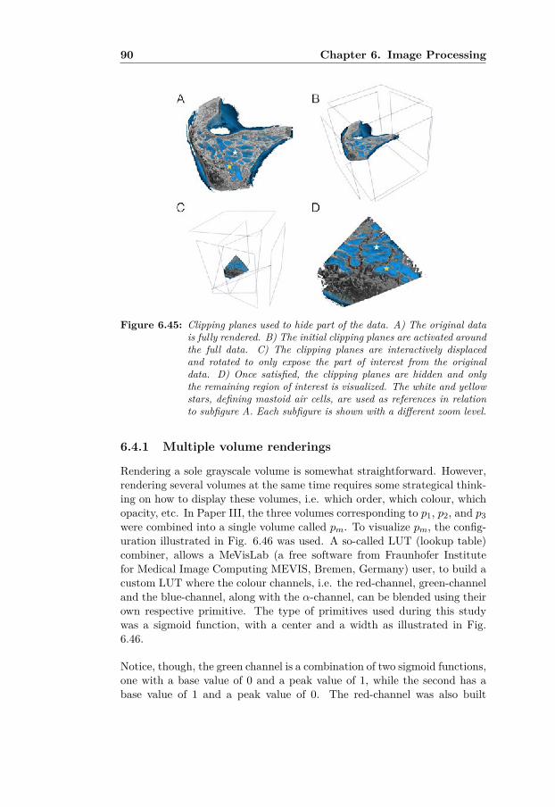
90 Chapter 6. Image Processing
Figure 6.45: Clipping planes used to hide part of the data. A) The original datais fully rendered. B) The initial clipping planes are activated aroundthe full data. C) The clipping planes are interactively displacedand rotated to only expose the part of interest from the originaldata. D) Once satisfied, the clipping planes are hidden and onlythe remaining region of interest is visualized. The white and yellowstars, defining mastoid air cells, are used as references in relationto subfigure A. Each subfigure is shown with a different zoom level.
6.4.1 Multiple volume renderings
Rendering a sole grayscale volume is somewhat straightforward. However,rendering several volumes at the same time requires some strategical think-ing on how to display these volumes, i.e. which order, which colour, whichopacity, etc. In Paper III, the three volumes corresponding to p1, p2, and p3were combined into a single volume called pm. To visualize pm, the config-uration illustrated in Fig. 6.46 was used. A so-called LUT (lookup table)combiner, allows a MeVisLab (a free software from Fraunhofer Institutefor Medical Image Computing MEVIS, Bremen, Germany) user, to build acustom LUT where the colour channels, i.e. the red-channel, green-channeland the blue-channel, along with the α-channel, can be blended using theirown respective primitive. The type of primitives used during this studywas a sigmoid function, with a center and a width as illustrated in Fig.6.46.
Notice, though, the green channel is a combination of two sigmoid functions,one with a base value of 0 and a peak value of 1, while the second has abase value of 1 and a peak value of 0. The red-channel was also built

6.4 Volume rendering 91
Figure 6.46: Schematic representation of the volume rendering scheme used inPaper 3 to illustrate pm.
with a sigmoid function with a base value of 1 and a peak value of 0.These primitives can be thought as a lowpass filter for the red-channel, aband-pass filter for the green-channel, and a high-pass filter for the blue-channel. Contrary to the RGB channels, the alpha-channel could onlybe built using a piecewise linear function, where control points could beadjusted accordingly.
The grayscale values from the resulting volume pm, ranging from 0 to 1could then be assigned a colour with red for tubular structures, greenfor isotropic structures, and blue for the planar structures and interme-diate colours between the three cases. Note that pm was multiplied witha thresholded version of the original micro-CT data, where only the bonewas segmented so as to only visualize pm within the bone and not for theoverall data. A downside while using this visualization scheme is the man-ual assignment of the three colour channels. Selecting the wrong center andthe wrong width of the sigmoid functions will lead to a misinterpretationof the structures from pm. A positive aspect of this method, however, is itsrelatively fast rendering since only two volumes are loaded.
Another type of visualization consists of letting p1, p2, and p3, govern thecolouring. Opting for this solution implies converting each of the cases p1,p2, and p3 into a RGB volume, and blend their respective contribution ina LUT combiner. However, similarly to the first scheme, Fig. 6.46, theα-channel could only be built using a piecewise linear function with con-trol points. The advantage of using this second scheme is the direct useof p1, p2, and p3 without having to create pm. A solution was to save thefinal RGB volume into a file and to later visualize it using a very basic

92 Chapter 6. Image Processing
volume rendering scheme, see Fig. 6.47. Another advantage is the possi-bility to create a combination of the cases, such as p1 & p2 or p1 & p3, orp2 & p3. This second advantage allows to qualitatively assess the correla-tion between the three cases. The inconvenient part of this configurationis the loading of five volumes, corresponding to the three cases and the twograyscale volume, i.e. the volume representing the λ1 and the original vol-ume for the masking. The time used for the computer to assign each voxelthe contribution from p1, p2, and p3 was also a negative point. Due to amore accurate representation, the second scheme was preferred in relationto the first scheme, previously used in Paper 3.
Figure 6.47: A different schematic representation of the volume rendering thatcan be used to illustrate pm, by simply loading the three volumes p1,p2, and p3, rescale them from 0 to 1 and convert them to a LUTmapping before being combined into a final LUT.
It is sometimes also desired to for instance show the complete result, whilerendering a limited part from the original data the computations are basedon. Two possible solutions are proposed. A first solution is illustrated inFig. 6.48, where the result from the analysis is rendered twice while theoriginal data is only rendered once.
A first set combines the original data together with a volume resultingfrom the analysis. This set is cached under the box named caching of stateduring rendering. The second set only involves the resulting volume. By

6.4 Volume rendering 93
Figure 6.48: Volume rendering scheme where the original data can be clippedwhile the secondary data remains fully rendered. To force the visi-bility of the secondary volume, it is present twice: under the cachingbox and the second one directly attached to the renderer.
clipping the first set, the volume containing the results from the analysisis kept untouched from the second set. Yet another solution is to preservethe volume containing the results from the analysis untouched but clippingcopies of the original data, as illustrated in Fig. 6.49. In addition to theregular clipping, the original data can also be masked with a binary volumecontaining only 1’s, on which simple geometrical objects are applied bysetting their inside as 0’s. The resulting binary volume is then multipliedwith the original volume and rendered on its own, while keeping the volumewith the results from the analysis untouched.
Illustrations of what can be obtained using such clipping is provided in Fig.6.50. In Fig.6.50(A and B), the clipping scheme presented in Fig. 6.48 isdemonstrated with two different types of geometry, see the box cavity inFig. 6.50(A) and the spherical cavity in Fig. 6.50(B). In Fig. 6.50(C),the original data is duplicated three times, one for displaying the result,another one for the front part, and one for the posterior part, all in allforming an inverting T shape. In Fig. 6.50(D), a mixture of a sphericalcropping of the binary masking together with the set of clipping boxes fromFig. 6.49 were used.
In the next chapter, a 3D shape analysis on the local thickness of themastoid air cells is further detailed. In this coming chapter, volume ren-

94 Chapter 6. Image Processing
Figure 6.49: Opposite to Fig. 6.47, the original volume is rendered twice whilethe secondary volume only once. A binary mask is used alongthe second rendering of the original data to crop simple shapes asspheres or boxes, allowing to display the secondary volume in thosecavities. The three dots to the left indicates that several volumescan be added along.
dering together with clipping and masking has been very useful, and formthe ground for a qualitative analysis presented in Paper VII along with adescriptive quantitative analysis.
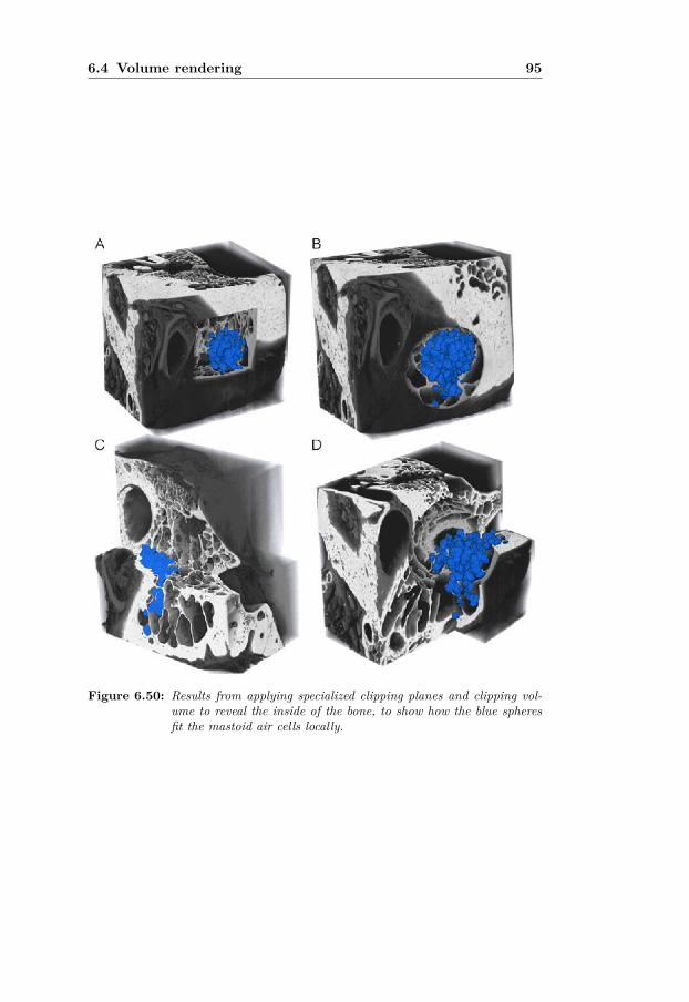
6.4 Volume rendering 95
Figure 6.50: Results from applying specialized clipping planes and clipping vol-ume to reveal the inside of the bone, to show how the blue spheresfit the mastoid air cells locally.


73D Shape Analysis
7.1 Introduction
This chapter provides a framework to answer the third question statedin the introduction of Chapter 4, namely what is the size of an air cell.Alhough the mastoid air cell system has been investigated as a very complexairspace, almost no reference has been found so far on determining the sizeof a singular air cell, and its possible variation in size. To the author’sknowledge, only the work by Virapongse et al. [86] has been investigatingthis problem directly. From observations on several mastoid air cells usingX-ray micro-CT scans, the size and shape of the mastoid air cells indeedvary dramatically.
Investigating the size of single air cells is not trivial. In [86], the authorsonly concentrated on so-called medium-sized cells corresponding to cellshaving a size, i.e. a diameter, ranging between 2mm to 5mm. Because ofthe limited resolution of their clinical x-ray CT scan, even after careful 3Dreconstruction, i.e. 0.3mm × 0.3mm × 1.5mm, they could only performa subjective analysis. All cells smaller than 2mm in size would be tooblurry to be correctly detected. In fact, they considered areas with smallair cells as regions with incomplete pneumatization, and warned the readerthat those regions should not be misunderstood as presence of a disease.The fact that the air cells were too small to be detectable on a clinical CTscanner is not a surprise, especially back in 1985. Presence of artefacts inx-ray CT scans, as previously introduced, leads to a false conclusion of thesmall air cells being hampered by mucosa thickening. Mucosa thickeningcan indeed happen, but it is not to be confused with physical limitationsfrom the scanner, such as resolution or artefacts.
Despite some misleading parts, the work by Virapongse et al. [86] haspointed out an important link between the size of an air cell, together withthe thickening of an inflamed mucosa, and the ability for the mastoid to

98 Chapter 7. 3D Shape Analysis
regulate negative pressure during pathology. This chapter aims at investi-gating the range of air cell sizes, and to observe how the cells are naturallydistributed in the mastoid.
The structure of this chapter is now described. Investigating the local sizeof the mastoid air cell system can be seen as a shape analysis problem,therefore a brief introduction to shape analysis is provided. As will be ex-plained further down, a series of maximally inscribed spheres are used asa shape descriptor of the local size. The maximally inscribed spheres areextracted along a medial axis, derived from a medial surface. The medialsurface is itself extracted via the use of structure tensor analysis appliedto a distance transform computed on the original data. Clustering of theextracted spheres, in the following referred to as medial balls, is then per-formed both in terms of size and location. While the size-based clusteringenables sorting the medial balls in terms of their diameters, location-basedclustering detects possible groupings of medial balls independent of theirdiameters. A further analysis is carried out by finding the proportion ofeach size-based cluster within each location-based cluster.
7.2 General definition of a shape
As defined by Kendall [41], a shape can be resumed by all geometricalinformation that remains when location, scale, and rotational effects arefiltered out from an object. There has been a gradual shift going fromshape description to shape representation.
Three-dimensional shape analysis deals with different types of challenges,ranging from the analysis of single complex shapes up to the analysis of anentire collection of shapes. Several main research directions, with special-ized mathematical tools have emerged, see the review in [8]:
• Feature detection: finding significant geometrical features in arobust manner. Differential geometry such as curvature or detect-ing salient points on the shape surface are common methods. Thesmoothness of the walls forming the mastoid air cells can be repre-sented using the curvature.
• Segmentation: decomposing a 3D model into significant parts. Themastoid air cells, or other parts of the temporal bone, can be decom-posed into different objects.
• Semantic labeling: assigning meaningful textual information to theconstituting parts of an object. The air cells can be labelled both interms of location and in relation to neighbouring structures, as definedby A. Allam and M. Tos [3, 85].

7.2 General definition of a shape 99
• Registration: finding correspondences between several objects. Com-pare the outer shape of the mastoid air cell system from several tem-poral bone specimens.
• Description: describing what an object looks like. Machine-understandablesignatures enable shape matching, shape retrieval, and shape classi-fication using histogram or distance from one point to another. Thedistance from the antrum to the terminal air cells in the mastoidcould be a description vector.
• Matching: comparing objects through similarity measures. From theshape descriptors, comparison can be done between several mastoidair cell systems (by comparing several features).
• Retrieval: finding an object in a large database. This is especiallyuseful in large repositories of 3D models. When performing a verylarge shape analysis of the mastoid air cell system using many speci-mens, it can be useful to retrieve the object from one specific case ina large repository.
• Classification and clustering: assigning an object to a specificclass. As will be explained later in this chapter, medial balls repre-senting the local size of the mastoid air cells are clustered accordingto their size and assigned a specific size class.
Although the entire set of items in the list is very appealing to investigate,the shape analysis in this study only concerns two items: description andclassification and clustering.
Zhang et al. [92] detail a classification of the different tools used in shaperepresentation and description. Because only one tool is used in this studyfor the shape description part, only the flowchart representing most of thecommon tool is illustrated in Fig. 7.1. From a description and representa-tion point of view, two main classes exist: contour-based and region-based.The difference between the two classes lies in the way the descriptors areextracted. In the contour-based method, the shape features are extractedfrom the contour of the object. In the case of the mastoid, the contour-based category would extract information from the contour of the mastoidair cells, i.e. the walls of the mastoid air cells. In the region-based category,the shape features are extracted from the overall volume forming the shape,i.e. all voxels forming the air cells including the contour voxels. When theshape needs to be represented in a discrete form, structural methods canbe used. When the shape has a smooth representation (implying continu-ity), global methods can be used instead. A further sub-classification canbe achieved by categorizing the method as either belonging to the spacedomain or to the transformation domain depending on how the shape de-scriptors are obtained, i.e. from the volume itself or from a transformation

100 Chapter 7. 3D Shape Analysis
such as the Euclidean distance transform [92].
Figure 7.1: Diagram resuming different subdivisions of shape analysis and thecategory the medial axis approach belongs to. The flowchart is in-spired from a review written by Zhang et al. [92].
Since the micro-CT scans used in our study are discrete volumes made ofvoxels, the methods to be used are structural. Global methods can alsobe used through interpolation, forming a more continuous representationof the data. In order to use maximum information from the data, theregion-based approach is preferred over the contour-based, which is validfor both representation and description. Among the structural region-basedmethods, one method was found to give the best results, namely the medialaxis representation.
The medial axis, originally created by Blum et al. [9] during the secondhalf of the twentieth century, allows a compact representation of the shape,while preserving sufficient information in order to reconstruct the shape ofthe original object as described by Kendall [41]. Obtained from the medialsurface, the medial axis can be used to find maximally inscribed spheres,locally representing the thickness of the mastoid air cells. Fig. 7.2 showsthe overall algorithm used in the current shape analysis, from the originalmicro-CT scan up to the obtention of the maximally inscribed spheres, i.e.medial balls, and how they are clustered based on their diameters, i.e. sizes,and their locations within the mastoid air cell system.
Examples of how medial balls along a medial axis can represent the sizeof the mastoid air cell system locally are provided in Fig. 7.3, for three

7.2 General definition of a shape 101
Figure 7.2: Flowchart explaining the extraction of the mastoid air cell size de-scriptor from the original micro-CT scan. A structural scheme basedon medial balls extracted from a medial axis and a medial surface isused. The shape descriptor is used in a classification and clusteringrepresentation. Note the semi-transparent box illustrating the extrac-tion of the medial balls from a skeleton using thinning instead, as apossible option which was used in this work for comparison purposes.
different cases. The colours represent the different range of sizes. Thethree cases represent air cells having different shapes. The first case, Fig.7.3(A), represents a finger-like elongated air cell similar to Fig. 5.4 but invertical orientation. A second case, where two air cells communicate via anarrow conduit, is illustrated in Fig. 7.3(B). Another pair of air cells, witha weakly defined transition or conduit, is presented in Fig. 7.3(C). Thesethree cases correspond to the three cases illustrated in Fig. 3.9.
When the mucosa is not inflamed, the three cases fully participate in the gasexchange. During inflammation, however, the mucosa lining the mastoidair cell walls will expand as previously explained in Chapter 3. Swelling ofthe mucosa may eventually lead to a full closure of the finger-like air cellin case Fig. 7.3(A), close the lower air cell in case Fig. 7.3(B), possiblyreducing the volume of gas of the airspace in case Fig. 7.3(C). For eachcase, i.e. A, B, and C, the medial axis is represented as illustrated inthe top row. In the bottom row, maximally inscribed spheres are placed

102 Chapter 7. 3D Shape Analysis
along the medial axis, and colour-coded based on their sizes from dark bluefor very small medial balls, up to purple for very large medial balls, withintermediate sizes respectively colour-coded as cyan, green, yellow, orange,red and magenta. In Fig. 7.3(A), the finger-link shape has a set of medialballs with a smooth variation in size. In Fig. 7.3(B), however, the sizevaries tremendously; from very small diameters up to very large diameters,with small spheres present between the two larger ones. Though the medialballs in Fig. 7.3(C) also vary in size, all the medial balls belong to a higherrange of diameters.
Figure 7.3: Equivalent maximally inscribed spheres based on the Euclidean dis-tance mapped onto the extracted medial axis.
From these examples, the diameters from all the medial balls provide awell-suited shape descriptor to represent the local thickness in a compactform. By clustering the medial balls in terms of size and location in 3D, itis possible to obtain a global map that may eventually be used in assessingthe level of occlusion of the mastoid air cells, either locally or globally.
Before investigating the clustering part, two important tools needed in theextraction of the medial balls from the original data are first covered: theEuclidean distance transform and the skeletonization. Though the Eu-clidean distance transform is used in this study, extraction of a skeletonis merely done by comparing purposes between existing methods to thescheme proposed in this study. The Euclidean distance transform is firstexplained.

7.3 Euclidean distance transform 103
7.3 Euclidean distance transform
The original concept of the Euclidean distance transform originates from H.Blum in the 60’s [9]. The transform is based on the grassfire principle, wherethe boundary of a grass landscape is set on fire. Under ideal conditions, thefire fronts advance only where there is grass, i.e. towards the centre of thelandscape and shock scaffolds appear, see Fig. 7.4. These shock scaffoldsappear where two fire fronts meet, and where the fire cannot go further.
Figure 7.4: Original and final steps of grassfire theory (on the top row) accordingto Blum’s theory which are given as analogy to a black rectanglesurrounded by a white border (lower left) and its Euclidean distancetransform (lower right) with the shock scaffolds displayed as dashedlines. The shock scaffolds are the skeletal elements of the black box.The black rectangle can represent a rough representation of an aircell on a micro-CT slice.
For each pixel in the image, or respectively voxel in the volume, the distancetransform assigns a number that corresponds to the distance between thatpixel/voxel and the nearest nonzero pixel/voxel in the data. In mathemat-ics, the Euclidean distance is defined as the straight-line distance betweentwo points in the Euclidean space. The Euclidean distance transform isusually performed on binary data, though a grayscale version exists [35].The grayscale representation is not used in this study.
For simple shapes like a parallelepiped, a sphere, or a cylinder, the Eu-

104 Chapter 7. 3D Shape Analysis
clidean distance transform is quite straightforward to mentally represent.Fig. 7.5 shows the Euclidean distance transform obtained on three simpleshapes: Fig. 7.5(A) a sphere, Fig. 7.5(B) a parallelepiped, Fig. 7.5(C)cylinders of different heights, and for a more complex structure built as acombination of spheres with different diameters together with an ellipsoid,see Fig. 7.5(D). Each shape is partially cut, so as to show its internal repre-sentation. The colour representation used in this example maps low valuesclose to the border as blue, while the largest values are represented as darkred, sometimes up to black. Notice how the how the central part of thethree cylinders changes as they differ in height. However, when the inves-tigated shape is more complex, its interpretation can become challenging.
Figure 7.5: Euclidean distance transforms applied to different shapes: A) asphere, B) a parallepiped, C) cylinders of different heights, and D)complex set of shapes.
To further illustrate the potential of the Euclidean distance transform andthe challenges when working with complex structures such as the airspacesin the temporal bone, Fig. 7.6 illustrates the Euclidean distance transformof the airspaces in a temporal bone. The bone is partially represented butlandmarks such as the lateral semi-circular canal, the utricle and a portionof the ear canal are represented. A partial representation of the mastoidair cells is also provided on the lower left side. As in Fig. 7.6, the colouringillustrates the distance from all air voxels to the bone voxels, the closer to

7.4 Skeletonization 105
the bone voxel the more blue it becomes and the further away from thebone voxels the more red it becomes.
Figure 7.6: Euclidean distance transform of the airspaces in the temporal bone.The lower right part represents part of the ear canal. The red spot tothe left represents the central cell of the mastoid air cell system, andis known to be large anatomically. The bony part surrounded by theEuclidean distance transform represents part of the incus head andshort process being part of the ossicular chain.
The Euclidean distance transform, can be used to extract the local thicknessof all airspaces. For instance, in Fig. 7.6, the red colouring present atthe lower left of the image, representing the mastoid air cells, indicatesthat there is a set of large cavities. Indeed, these large cavities form thebasis for the mastoid midline, with the antrum being prolongated in thecentral cells before splitting into smaller air cells. As will be shown laterin this chapter, the Euclidean distance transform will be used to build acompact representation of the mastoid air cells used for the shape analysis.The notion of skeletonization, and how to extract the skeleton from theEuclidean distance transform, is explained in the following section.
7.4 Skeletonization
Four main classes of skeletonization methods exist: (1) thinning methods,(2) distance-field based methods, (3) general-field methods, and (4) geo-metric methods. There is a plethora of methods used in each of theseskeletonization techniques. Their description is beyond the scope of thisthesis, but interested readers can find several surveys, [67, 82]. Only thetwo first methods, i.e. the thinning method and the distance-field based

106 Chapter 7. 3D Shape Analysis
method, are considered in this thesis. The skeleton implemented in PaperVI is based on the Euclidean distance transform, and therefore belongs tothe distance-field skeletonization based method. The thinning method usedin Paper VI, for comparison purposes, is based on the thinning method. Be-fore providing more details about the medial axis approach implemented inthis study, the skeleton based on thinning-based method is first described.
The skeleton is directly extracted from a binary representation of the mas-toid air cell system, obtained by thresholding explained in Sec. 6.1.1. Theskeleton is obtained by an iterative morphological thinning procedure of theforeground of the obtained binary representation, where for each iterationa layer of boundary voxels is removed. Despite the need for multiple teststo respect certain conditions, this procedure is relatively straightforward.
Depending on the size of the binary structure to extract the skeleton from,this technique can take a large amount of time, in the order of an hourfor a complete temporal bone from an X-ray micro-CT scan. A downsidewith such a skeletonization technique is the presence of loops which in 3Dcan also form blobs, i.e. an enclosed cavity. Such loops break one of theelementary rules of a true skeleton. Some methods propose to break theseloops by cutting the shortest branch. Also, presence of noise in the originaldata can have a large effect on the extracted skeleton.
Any perturbation at the border of the binary representation will be prop-agated along the morphological thinning, leading to spur branches. Spurbranches can be removed as a post-processing step, but when true finestructures are present at the borders, a decision on whether a branch is aspur branch to remove, or a branch to preserve, becomes challenging if notimpossible [68]. A typical example of a skeleton obtained from the thinningmethod is illustrated in Fig. 7.7.
Beside the presence of noise, because this type of skeleton is discrete, itmay eventually be locally represented by two voxels instead of only onevoxel, breaking one of the fundamental rules for being characterized as askeleton [72]. More practically, such a two-voxel representation may leadto further errors when attempting to extract maximally inscribed sphereslocally, implying new conditions on which one of the two voxels to preserve.Similarly, the junctions of the skeleton are often represented by more thantwo voxels, often up to four or fives voxels besides the junction voxel andits neighbouring voxels directly attached to it. For simpler shapes, thesedrawbacks can be corrected quite easily, but in the presence of very complexstructures, such as the mastoid air cell system, correcting these issues wouldbe very time consuming.
The second class of skeleton is based on the distance transform. As in-troduced in the previous section, shock scaffolds are formed where the fire

7.4 Skeletonization 107
Figure 7.7: A 3D skeleton of the MACS obtained via binary thinning down toone voxel size branches. From the three windows, further zoomed tothe right, multiple unuseful branches along with blobs are pointed out.
fronts meet. These intersections form a medial axis. As represented inFig. 7.8, the shock scaffolds can have multiple shapes: a surface for theparallelepiped (Fig. 7.8(d)), a point for the sphere (Fig. 7.8(e)), and a linefor the cylinder (Fig. 7.8(f)).
However, these medial axes are obtained by finding a global maximum foreach of the cases. When looking at local maxima, the medial axes becomemore complex in shape. In Fig. 7.8(a), the surface is augmented by thepresence of eight branches joining each corner of the surface to each of thecorner. In Fig. 7.8(c), a conic shape is added to both extremities of themedial axis. Only the case with the sphere, in Fig. Fig. 7.8(e) does notchange since only the place where the shock scaffold is present is at thecentre of the sphere. To further help understanding the difference betweenFig. 7.8(a,b,c) and Fig. 7.8(d,e,f), the EDT is also provided in colours. InFig. 7.8(a), the Euclidean distance along each of the eight branches willvary from low value (blue) to the high values (red). The same applies inFig. 7.8(c), where the base of two conic shapes will correspond to low values(blue) and where their respective tip will have the highest value (red). Inthe case of Fig. 7.8(d,e,f), a very compact representation of the originalshape is obtained, but its reconstruction will be incomplete. However, in

108 Chapter 7. 3D Shape Analysis
Figure 7.8: Natural medial axis formed by the shock scaffolds from three Eu-clidean distance on three simple cases: parallepiped (a, d), a sphere(b, e), and a cylinder (c, f). In (a, b, c) the complete medial axis,obtained by detecting all local maxima, is represented with the blacklines and further pointed out by the white arrows for each of thecases. In (d, e, f) only the global maximum was used to detect themedial axis. A cosine square of the EDT was used to represent thefire fronts at different levels, in order to visualize the shock scaffoldsin each of the three cases. The fire fronts are represented with thegray surfaces seen as shells around the medial axis obtained from theglobal maxima. Clipping planes were used in order to visualize theinner parts of the three shapes.
the case of Fig. 7.8(a,b,c), the reconstruction will be more accurate. Itshould be noted that the scaffolds are graphically represented using thecosine square of the Euclidean distance transform, i.e. cos2(EDT ), as graysurfaces mixed with the coloured Euclidean distance transform, as visible inFig. 7.8. In the present work, reconstruction of the mastoid air cell systemfrom the medial axis is not desired. However, because a good representationof the mastoid air cell system using medial balls is desired, detection of localmaxima becomes necessary.
As will be seen later in this thesis, the medial axis is, in this study, ex-tracted from the Euclidean distance transform using more advanced imageprocessing, e.g. quadrature filters and structure tensor analysis, to allow amore robust detection of the local maxima. Also, when compared to the

7.5 Medial surface 109
morphological thinning, extracting a skeleton from a distance transformoutput allows a more continuous representation, and corresponds more toa curve skeleton than a discrete skeleton. In the case of a morphologicalthinning, an interpolation scheme is needed in order to produce a curveskeleton from its discrete representation.
In the next section extraction of the medial surface, used to extract themedial axis implemented in Paper VI, is further detailed.
7.5 Medial surface
From the enhanced data, the Euclidean distance transform is estimated,with the boundaries of the mastoid air cells used as starting points. Theoutput of the Euclidean distance transform is then used to estimate thestructure tensor. The resulting tensor is denoted Tms with ms standing formedial surface. The quadrature filters used to estimate Tms are the same asfor estimating the structure tensor in the enhancement scheme. In addition,the local phase is estimated along with the norm of the structure tensor.To further help the reader’s understanding, the eigenvalues obtained fromTms are illustrated in decreasing order from left to right in Fig. 7.9. Ascan be observed, the largest eigenvalue λms1 already provides informationabout the medial surface. The local phase helps removing the responsesfrom the boundary.
Figure 7.9: Eigenvalues of the structure tensor estimated from the Euclidean dis-tance transform, shown in decreasing order, for a mastoid air cellsystem: λms1, λms2, and λms3.
The local phase, briefly introduced in Sec. 6.2.1, is then used to sepa-rate the irregularities from the Euclidean distance transform from the data

110 Chapter 7. 3D Shape Analysis
boundaries. The local phase, rewritten in terms of the real and imaginarypart of the quadrature filter response, is estimated as
ϕloc = arctan
(∑k ‖ Im{qk}‖∑k Re{qk}
), (7.1)
with Re {qk} and Im {qk} being the real and imaginary parts of the quadra-ture filter responses in the k directions. To make use of the informationprovided by the local phase, a phase-based weighting factor wϕ is computedas
wϕ = cos
(ϕloc
2
)γloc
, (7.2)
with γloc equal to 4 in the present work. A simplistic illustration of thelocal phase, resulting from Eq. 7.2 is provided in Fig. 7.10. Signals withdifferent widths, but with a similar magnitude, are illustrated in (a), whilesignals with different width and magnitude in (b). In all cases, the localphase detects the local maximum, as pointed out with the red circles. Whenusing the Euclidean distance transform, the local phase will detect the localmaxima resulting from the collision of the shock scaffolds.
Figure 7.10: Detection of the local maximum for signals with different widths (a)and also having different magnitudes (b).
The medial surface is then obtained by multiplying the norm of the struc-ture tensor Tms with Eq. 7.2, i.e.
Msurf = ‖Tms‖wϕ. (7.3)
An illustration of the medial surface before applying the local phase isprovided in Fig. 7.11. The medial axis is represented in green, whilethe remaining part of the volume is represented in blue and considered asbackground. A zoom is added at the border of one air cell, to illustrate theneed to remove unwanted ridges. To highlight the medial surface further,the transfer function used to represent the temporal bone corresponds tothe transfer function introduced in Paper II.

7.5 Medial surface 111
Figure 7.11: Volume rendering of the medial surface (green) before removal ofunwanted ridges via the local phase. The remaining part of ‖Tms‖is represented as blue. A zoom is also provided to illustrate theunwanted ridges from the boundaries. Source: [14].
Once the local phase is applied to ‖Tms‖, the medial surface is extractedand illustrated together with the original data for two different angles inFig. 7.12.
Figure 7.12: Volume rendering of the medial surface represented in yellow, alongwith the original data for two different orientations on the samebone specimen, (left) from a lateral view and (right) from a posteriorview. Clipping planes were used to reveal the inner part of the bone.
The medial surface output volume is illustrated in Fig. 7.2, as the graybox with the number 1 next to it. Using the idea of extracting the medial

112 Chapter 7. 3D Shape Analysis
axis from the medial surface from [63], the medial axis is then obtained asexplained in the following.
7.6 Medial axis
The medial axis can be directly extracted using
Maxis = pms2 = λms2 − λms3λms1
, (7.4)
where λms1, λms2, and λms3 are the eigenvalues of ‖Tms‖. Further, it wasdecided to perform a structure tensor analysis on ‖Tms‖, so as to gainmore flexibility on the content of the medial axis. The estimated structuretensor is called Tma standing for medial axis. The eigenvalues obtainedfrom ‖Tma‖ are then λma1 ≥ λma2 ≥ λma3 ≥ 0. Using
pma1 = λma1 − λma2λma1
, pma2 = λma2 − λma3λma1
, pma3 = λma3λma1
, (7.5)
along with pms1 and pms3, the medial axis can be extracted using
Maxis = (pma1 − αma pms1) + pma2 + βma (pms3 + pma3) , (7.6)
with αma = 0.75, and βma = 0.01. The parameters αma and ςma respec-tively allow the addition of a planar and an isotropic components to themedial axis. Although slightly violating the properties defining a skeletonor a medial axis as stated in [82], preserving a certain amount of planarand isotropic part from the medial surface, together with the tubular partof the medial axis, the medial axis has better continuity. Note that usinga combination of the eigenvalues from both tensors, Tms and Tma, canalso be used to create a more sparse medial axis with less points along itscourse. Because the two tensors are computed over the entire volume, it isnecessary to restrict the information along the medial surface. Therefore,the medial axis is finally calculated as
Maxis = MaxisMsurf . (7.7)
An illustration of the obtained medial axis is provided in Fig. 7.13. Toassess the quality of the skeleton, another skeletonization scheme (availableover the Matlab file exchange (Mathworks, USA)) was used [50]. Thepackage will in the following be referred as Skeleton3D. In Fig. 7.13(left),the medial axis extracted using the present scheme is presented, while Fig.7.13(right) presents the skeleton resulting from Skeleton3D.
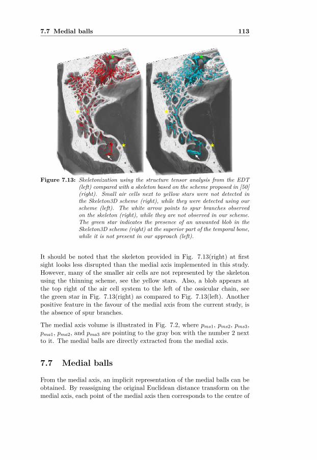
7.7 Medial balls 113
Figure 7.13: Skeletonization using the structure tensor analysis from the EDT(left) compared with a skeleton based on the scheme proposed in [50](right). Small air cells next to yellow stars were not detected inthe Skeleton3D scheme (right), while they were detected using ourscheme (left). The white arrow points to spur branches observedon the skeleton (right), while they are not observed in our scheme.The green star indicates the presence of an unwanted blob in theSkeleton3D scheme (right) at the superior part of the temporal bone,while it is not present in our approach (left).
It should be noted that the skeleton provided in Fig. 7.13(right) at firstsight looks less disrupted than the medial axis implemented in this study.However, many of the smaller air cells are not represented by the skeletonusing the thinning scheme, see the yellow stars. Also, a blob appears atthe top right of the air cell system to the left of the ossicular chain, seethe green star in Fig. 7.13(right) as compared to Fig. 7.13(left). Anotherpositive feature in the favour of the medial axis from the current study, isthe absence of spur branches.
The medial axis volume is illustrated in Fig. 7.2, where pms1, pms2, pms3,pma1, pma2, and pma3 are pointing to the gray box with the number 2 nextto it. The medial balls are directly extracted from the medial axis.
7.7 Medial balls
From the medial axis, an implicit representation of the medial balls can beobtained. By reassigning the original Euclidean distance transform on themedial axis, each point of the medial axis then corresponds to the centre of

114 Chapter 7. 3D Shape Analysis
a maximally inscribed sphere, with a radius corresponding to the Euclideandistance transform value. These medial balls are obtained by combining themedial axis with the Euclidean distance obtained from the enhanced data,and are illustrated in gray in Fig. 7.2 with the number three next to it.Clustering can then be used to classify the medial balls according to theirsizes or locations, clustering based on the size is first approached.
Figure 7.14: Medials balls representing the maximally inscribed spheres withinthe mastoid air cells.
The medial balls can then be used as a shape descriptor and in a clusteringscheme, to find any specific patterns in the volume formed by the medialballs as represented in Fig. 7.14. Such a pattern could, in terms of themastoid, be a local aggregate of air cells of a certain size range, or whetherthe air cells form natural groups as previously discussed in Chapter 3. Toachieve a clustering analysis, two tools need to be employed. One tool is theK-means clustering, which is used to divide the medial balls into clusters.The second tool is the convex hull, which is related to the enclosed regionscontaining the clustered medial balls. These two tools are now described.
7.8 K-means clustering
Kmeans or K-means is a partitioned clustering algorithm that tries to find Knon-overlapping clusters, each represented by their centroids. The K-meansclustering process can briefly be described with the following steps. First, Kcentroids are initially manually selected, often based on a-priori knowledgeabout the data. In the case of the mastoid air cells, the number of regions

7.9 Convex hull 115
defined by A. Allam and M. Tos is a good starting point [3, 9]. Everypoint in the data is then assigned to the closest centroid. The collection ofpoints assigned to a centroid defines a cluster. The centroid of each clusteris then updated based on the points assigned to that cluster. This processis repeated until the clusters are stable. In relation to the medial balls, thepoints represent their respective centres. More information about K-meansclustering can be found in [90].
An important point to add, though, is how to select the number of clustersto divide the data into. While it is possible to select a predefined number ofclusters using some a-priori knowledge about the data, a repeated iterationof the K-means algorithm with different cluster values does not always giveconsistent classification, visible when observe their convex hulls changingshape over iterations. If the results from manual selection of the numberof clusters is not satisfactory, it is possible to use the Calinski-Harabaszcriterion, also known as the variance ratio criterion, to get the optimalnumber of clusters [10]. The notion of a good clustering depends on whatneeds to be evaluated. Attaining high intra-cluster similarity and low inter-cluster similarity is the ultimate goal of clustering. It should be notedthat a high value from this criterion does not necessarily lead to a naturalclustering of, for instance, the air cells in the mastoid.
The notion of convex hull was introduced earlier. In the next section, abrief definition of the convex hull is provided.
7.9 Convex hull
To visualize the obtained clusters, a convex hull is determined for eachcluster. A complete definition of a convex hull is beyond the scope ofthis thesis, but interested readers are referred to [7]. Its basic definition isresumed in the following.
A convex hull, in 2D, is defined as the smallest convex polygon P thatcontains all the points of a set S. A polygon P is said to be convex if: (1)P is non-intersecting; (2) for any two points p and q on the boundary ofP , the segment pq lies entirely inside P . In 3D, given a set of n points P ,the convex hull CH(P ) is the smallest polyhedron, so that all elements ofP lie inside and at the boundary of the polyhedron. An example of a 3Dconvex hull is illustrated in Fig. 7.15.
K-means clustering is often used for N-dimensional data, requiring a defini-tion of a convex hull in N-dimensions. Fortunately, as the data used in thiswork is three-dimensional, a 3D convex hull representation of the obtainedclasses can help to assess their variation in shape and size over the selectednumbers of clusters, as explained in the next section.

116 Chapter 7. 3D Shape Analysis
Figure 7.15: A 3D convex hull (right) for a set of random 3D points (left).
7.10 Clustering the air cells
An example of clustering the temporal bone is illustrated in Fig. 7.16, whereeach cluster is represented by its convex hull. Each cluster is assigned adifferent colour for better distinction among the clusters. Each convex hullis rendered semi-transparent to reveal the centroid. It should be notedthat the clustering in this example is the result of an earlier test where thenumber of clusters to be found was chosen to be 14. Within each cluster,the points belonging to the medial axis are used as the centres for themedial balls as illustrated in Fig. 7.15. When comparing to the regionsdefined by A. Allam and M. Tos [3, 85], the resulting clusters representedby their convex hulls, seem to correspond to the natural grouping of cellsas observed in exposed temporal bones.
At least two types of clustering are possible: one clustering based on thesize of the medial balls (defined by their diameters), and a second clusteringbased on the locations of the medial balls in the mastoid air cell system.The two proposed clustering approaches are now detailed.
7.10.1 Clustering in relation to size
The first clustering approach is aimed at defining a set of size ranges. Usingthe equivalent radii alone as a 1D vector, the K-means clustering can classifythe vector into several classes based on a predetermined number of clusters.To avoid confusion with the location-based clusters, the eight size-basedclusters are named from CS1 up to CS8, with the letter S to emphasize thatit relates to size-based clusters. The eight volumes, each corresponding toa separate volume, are represented by the gray boxes CS1 and CS8 with

7.10 Clustering the air cells 117
Figure 7.16: Example of a segmentation using K-means clustering. The tempo-ral bone clusters are represented by semi-transparent convex hullsrevealing the cluster centroids (red stars). Each cluster is repre-sented with a different colour for better interpretation. Note thatthis example is based on 14 clusters with the exclusion of the tym-panum.
the number 4 on its left in Fig. 7.2. To obtain a detailed grouping of themedial balls, and after using the Calinski-Harabasz criterion, the number ofclusters was chosen to be eight, where: blue represents the smallest medialballs, cyan represents a range of small medial balls, green corresponds tomedium small medials balls, yellow is dedicated to mediummedial ball sizes,orange defines the medium large medial balls, and where red magenta andpurple emphasise the large up to the largest medial ball sizes.
In Fig. 7.17, the original data, Fig.7.17(a), and renderings of each the eightsize clusters are provided; each rendered separately with a semi-transparentrepresentation of the bone. While Fig.7.17(a) is partially clipped, the semi-transparent original data for each of the remaining subfigures is fully rep-resented. As can be seen in Fig. 7.17, the K-means clustering was able tocluster the medial balls based on their sizes, i.e. diameters. By compar-ing the different size-based clusters, the smallest medial balls seem to bemore concentrated towards the superior part of the bone, see Figs. 7.17(b),7.17(c), 7.17(d). The clusters capturing the larger medial balls, i.e. CS6 toCS8, show a clear separation between the central airspace in the proximityof the antrum, see Figs. 7.17(g), 7.17(h), 7.17(i). Note that this symmetryis often used as the midline of the mastoid, from the antral cells down tothe apical cells at the lower part of the bone.
The remaining medial balls seem to be well spread over the whole mastoid,see Figs. 7.17(e) and 7.17(f), though a groove seems to already appearin Fig. 7.17(f), announcing a separation between the lower part from thesuperior part of the mastoid air cell system. When particularly observing
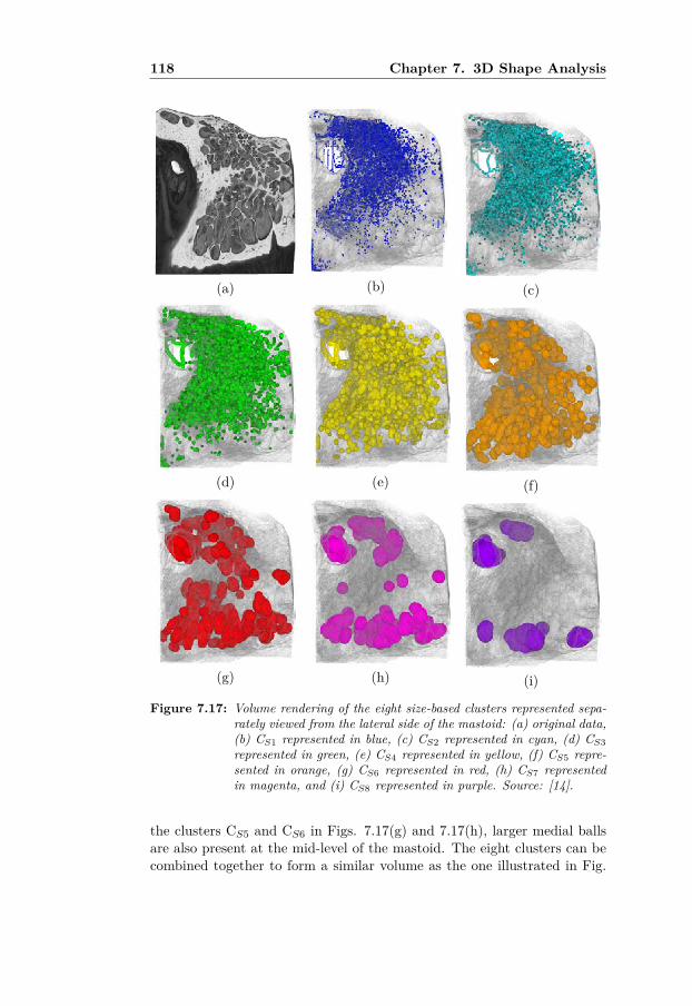
118 Chapter 7. 3D Shape Analysis
(a) (b) (c)
(d) (e) (f)
(g) (h) (i)
Figure 7.17: Volume rendering of the eight size-based clusters represented sepa-rately viewed from the lateral side of the mastoid: (a) original data,(b) CS1 represented in blue, (c) CS2 represented in cyan, (d) CS3represented in green, (e) CS4 represented in yellow, (f) CS5 repre-sented in orange, (g) CS6 represented in red, (h) CS7 representedin magenta, and (i) CS8 represented in purple. Source: [14].
the clusters CS5 and CS6 in Figs. 7.17(g) and 7.17(h), larger medial ballsare also present at the mid-level of the mastoid. The eight clusters can becombined together to form a similar volume as the one illustrated in Fig.

7.10 Clustering the air cells 119
7.14, with the exception that each medial ball is now coloured based onits size cluster as shown in Fig. 7.18. The combination of all clusters isrepresented in Fig. 7.18.
(a) (b) (c)
(d) (e) (f)
(g) (h) (i)
Figure 7.18: Volume rendering of different combinations of eight size-based clus-ters from the largest medial balls to the smallest one, to see howthe different size clusters relate to each others. Legend: (a) orig-inal data, (b) CS8, (c) CS8-CS7, (d) CS8-CS6, (e) CS8-CS5, (f)CS8-CS4, (g) CS8-CS3, (h) CS8-CS2, (i) CS8-CS1. Source: [14].

120 Chapter 7. 3D Shape Analysis
However, the relation between the cell sizes and their locations within themastoid is not captured when clustering the medial balls in terms of size.In the next subsection, a clustering analysis of the medial balls based ontheir 3D location is presented.
7.10.2 Clustering in relation to 3D location
Compared to the size-based clustering, clustering the medial balls basedon their 3D locations requires a more subtle selection of the number ofclusters. One option when choosing their grouping in 3D relates to an a-priori knowledge on how they are naturally grouped in the temporal bone.As proposed by M. Tos [85], a set of eleven groups can represent the mastoidair cell system. Because the tympanum and the inner ear structure, i.e. thecochlea and the vestibular system, are also present in the original data, onemore cluster was added leading to a total of 12 clusters to extract. As forthe size-based clusters, the location-based clusters are named as CL1 upto CL12, with L to emphasize that they relate to location-based clustering.CL1 up to CL12 are illustrated in Fig. 7.2 with the number 5 to the rightside of it.
Fig. 7.19 and Fig. 7.20 provide the location-based clusters from a lateralside and from a posterior view. The relations between the clusters shownin Fig. 7.19 and Fig. 7.20 to the regions described by A. Allam and M. Tos[3, 85] (as illustrated in Fig. 3.4), are shown in Table 7.1. For each cluster,the corresponding regions are provided as names, but also according to thelabel numberings in Fig. 3.4.
Description Labels inFig. 3.4
CL1 tympanum -CL2 antral, tegmental, zygomatic 1, 3, 4CL3 antral (medial), tegmental 1, 3CL4 antral (lateral), periantral 1, 2CL5 antral (medial), periantral 1, 2CL6 periantral, sinodural, superior retrosigmoid, medial persinusal 2, 5, 7, 8CL7 central (inferior), inferior retrosigmoid, perifacial (medial) 6, 9, 10CL8 central (inferior), inferior retrosigmoid, perifacial (lateral) 6, 9, 10CL9 perifacial (medial), apical (anterior) 10, 11CL10 perifacial (lateral), apical (anterior) 10, 11CL11 perifacial (lateroinferior), apical (anterior) 10, 11CL12 apical (posterior) 11
Table 7.1: Anatomical correspondence of the 3D location-based clusters from Fig.7.19 and Fig. 7.20 in relation to the regions defined by A. Allam andM. Tos ([3, 85]) as illustrated in Fig. 7.2. Source: [14].

7.10 Clustering the air cells 121
Size distribution histograms of each location-based cluster are provided inFig. 7.21. A common observation is the fact that all distributions havea positive skewness, except for the last histogram, see Fig. 7.21(l). Theskewness is to be expected since, as visible in Fig. 7.19(a, b, c) for theposterior view and Fig. 7.20(a, b, c) for the corresponding superior views,there are many more small medial balls compared to larger ones, thus lead-ing to a shift of the mean towards the smaller cells. Also, as clearly visiblein Fig. 7.21(g), the histograms often contain a mixture of distributions,which makes sense since several size-based clusters are combined into eachof the location-based clusters.
The proportion of each size-based cluster in each location-based cluster isrepresented as a series of twelve pie charts, see Fig. 7.22. As previouslyexplained, CL1 corresponds to the tympanum and stands on its own. How-ever, as highlighted by the red rectangle, clusters CL2 up to CL4 have verysimilar patterns in terms of proportions. There is a dominating proportionof cells with a size range of type CS2 and CS3. Similarly, CL5 up to CL7present common features with more small medial balls than in the pre-vious rectangle, but more medial balls of type CS3 and CS6. CL8 has awell distributed amount of each size-based cluster with a lower amount ofCS8. No CS9 is present though. Cluster CL9 could be included in the bluerectangle but its lower amount of CS5 and CS7 implies CL9 to be on itsown. The same applies for CL10 though it contains all types of size-basedclusters. Clusters CL11 and CL12 are very similar in terms of proportionsand were therefore paired together within the green rectangle. CL11 andCL12 correspond to the apical cells. A black arrow above CL1 is aimed athelping the reader to visualize the chronology of appearance from CS1 upto CL12. The star added to the cluster title from CL3 up to CL9 indicatesthat no medial balls of size-type CS9 was found in those clusters.
A more clinical interpretation can be provided by these results. When themucosa lining the mastoid air cell system is inflamed, it is expected thatregions with a narrow space such as small air cells, narrow conduits, orsmall protrusions will be filled by mucosa, thus leading to a much lowersurface area exposed to gas exchange as compared to the volume of gaswithin the air cells. Depending on the thickening of the mucosa, a firstapproach could in the future be to remove, for instance, all medial ballsbelonging to CS1 and CS2 from all location-based clusters CL1 up to CL12,and observe the impact on the local pneumatization. For clusters CL2 up toCL4, removing CS1 and CS2 would reduce their capacity by more than 50%. For clusters CL5 up to CL7, removing CS1 and CS2 would reduce theircapacity by more than 45 %, while for CL8 CL11 and CL12, the reductionwould be slightly lower with about 40 %. In the remaining set of clusters,that is CL1, CL9, and CL10, the reduction would be down by a factor of 4.

122 Chapter 7. 3D Shape Analysis
Using simulation, it may be possible to assess the effect of mucosal thick-ening on the gas exchange rate, and thereby on the negative pressure reg-ulation.
In the next chapter, an overview of the published papers related to thisthesis is provided.

7.10 Clustering the air cells 123
(a) CL1 (b) CL2 (c) CL3
(d) CL4 (e) CL5 (f) CL6
(g) CL7 (h) CL8 (i) CL9
(j) CL10 (k) CL11 (l) CL12
Figure 7.19: Volume rendering of the twelve 3D location-based clusters togetherwith a semi-transparent representation of the original data from alateral view for better co-localisation. Source: [14].

124 Chapter 7. 3D Shape Analysis
(a) CL1 (b) CL2 (c) CL3
(d) CL4 (e) CL5 (f) CL6
(g) CL7 (h) CL8 (i) CL9
(j) CL10 (k) CL11 (l) CL12
Figure 7.20: Volume rendering of the twelve 3D location-based clusters togetherwith a semi-transparent representation of the original data from aposterior view for better co-localisation.

7.10 Clustering the air cells 125
(a) CL1 (b) CL2 (c) CL3
(d) CL4 (e) CL5 (f) CL6
(g) CL7 (h) CL8 (i) CL9
(j) CL10 (k) CL11 (l) CL12
Figure 7.21: Size distribution for each of the location-based cluster. Legend: x-axis represents the size, i.e. diameter, of the medial balls in mm;the y-axis represents the number of medial balls found per size bin.

126 Chapter 7. 3D Shape Analysis
Figure 7.22: Pie charts representing the proportions of each size-based clusterwithin each of the location-based cluster. Source: [14].

8Summary of Papers
8.1 Introduction
This chapter provides brief summaries of the enclosed papers. Most of thematerials presented in the papers have been covered in the first part ofthe thesis. From the previously stated observations, two main paths weretaken. Due to the rare availability of X-ray micro-CT scans of completetemporal bones, especially including the mastoid bone, it was consideredvery important to investigate the surface area and volume occupied by theair in the mastoid air cell system, and compare the results obtained withprevious studies (most of them relying on clinical CT scans).
Paper I relates to this part of the study. During the scanning of the tempo-ral bones at the Department of Physics and Astronomy, Ghent (Belgium),while assessing the quality of the scans using volume rendering, togetherwith Manuel Dierick and Elin Pawels, micro-channels running in the corticalpart of the bone were discovered. As previously introduced, this discov-ery raised many questions. Therefore a divergence from the analysis of themastoid air cells was unavoidable. Due to their complex structures, and thefact that their size is close to the scan resolution, further image processingwas needed to better understand their geometrical inter-relation. PapersII, III, and IV relate to this part of the study.
Though further investigation of these micro-channels is relevant, the analy-sis of the mastoid air cells, not as as a single system but as separate entities,was at this stage considered a natural extension of the primary work. Inorder to extract relevant metrics, such as the size distribution or the waythe cells are grouped together in the mastoid, a preliminary shape analysiswas designed to investigate the complete range of sizes the air cells have.
The analysis was applied on one complete temporal bone. In order to obtaina simpler representation of the air cell system, a new way of extracting amedial axis from an Euclidean distance transform was devised, and further
128 Chapter 8. Summary of Papers
used to extract medial balls from which the local size was estimated. Usingthe medial balls, it was then possible to study the local variation in size ofthe mastoid air cells and assess whether the size variation correlates withthe regions defined by A. Allam and M. Tos, [3, 85]. Paper V presents thenovel way of extracting the skeleton from the Euclidean distance transform,while Paper VI provides improvements on obtaining the medial axis anddetails the clustering of the obtained medial balls in terms of size andlocation. These contributions, though not necessarily all relevant duringclinical practice, are believed to facilitate the understanding of the mastoidin terms of anatomy, but also in terms of its physiological role. Each papercontribution is presented separately as follows.
8.2 Paper I
Determination of the mastoid surface area and volume basedon micro-CT scanning of human temporal bones. Geometricalparameters depend on scanning resolutions. Olivier Cros, HansKnutsson, Mats Andersson, Elin Pawels, Magnus Borga, Michael Gaihede.Hearing Research Special Issue MEMRO 2016, Volume 340, pages 127-134,2016.
In this paper we describe the determination of the surface area to volumeratio, which may indicate that the mastoid air cell system is adapted togas exchange, and assess the influence of the resolution on these parame-ters by downsampling the data four times. The surface area and volumewere obtained through image processing tools commonly found in the fieldof hearing research, for comparison purposes though adjusted to the highresolution of the micro-CT scans. The current study found significantlylarger surface areas and higher surface area to volume ratios than foundin previous studies, performed at a limited resolution of around 625µm(commonly found in clinical CT scanners). The statistics resulting fromthis study are important for a more accurate modelling of the middle earphysiology.
8.3 Paper II
Micro-channels in the mastoid anatomy. Indications of a separateblood supply of the air cell system mucosa by micro-CT scanningOlivier Cros, Magnus Borga, Elin Pauwels, Joris Dirckx and Michael Gai-hede. Hearing Research. Volume 301. pages 60-65, 2013.
This paper describes a discovery within the temporal bone named afterits structural shape, i.e. the micro-channels. A qualitative analysis using

8.4 Paper III 129
volume rendering first demonstrated the presence of these micro-channels,connecting the surface of the compact bone directly to the mastoid air cells,as well as forming a network of connections between the air cells. A quan-titative analysis on 2D slices was then employed to determine the averagediameter of these micro-channels, as well as their density at a localizedarea. These channels are believed to house a separate vascular supply forthe mastoid mucosa. This study further helps improving our knowledge ofthe physiological properties of these micro-channels, which may have impor-tant implications for understanding the pressure regulation of the middleear.
8.4 Paper III
Structural analysis of micro-channels in human temporal boneOlivier Cros, Michael Gaihede, Mats Andersson, Hans Knutsson. An-nual meeting of the IEEE International Symposium on Biomedical Imaging(ISBI), New York, United States of America, pages 9-12, April 2015.
In this paper a preliminary structural analysis of the micro-channels wasimplemented using structure tensor analysis. The eigenvalues obtainedfrom the estimated local structure tensor were used to build probabilitymaps representing planar, tubular, and isotropic tensor types. A visualinterpretation of the three different tensor structure types was possibleby assigning a respective RGB colour, and the full structure tensor wasrendered along with the original data, to allow a smooth transition betweenthe three tensor types. Such a structural analysis has provided new andrelevant information about the micro-channels, but also their connectionsto the mastoid air cells.
8.5 Paper IV
Enhancement of micro-channels within the human mastoid bonebased on local structure tensor analysis. Olivier Cros, Anders Ek-lund, Michael Gaihede, Hans Knutsson. IEEE Sixth International Confer-ence on Image Processing Theory, Tools and Applications (IPTA’16), Oulu,Finland, December 2016.
In this paper enhancement of the micro-channels was implemented usingstructure tensor analysis based on the framework in Paper III. In order toassess the quality of the results obtained with our scheme, a qualitativeanalysis was carried out followed by a comparison with another enhance-ment scheme. The enhanced micro-channels appeared more well-defined.

130 Chapter 8. Summary of Papers
8.6 Paper V
Surface and curve skeleton from a structure tensor analysis ap-plied on mastoid air cells in human temporal bones. Olivier Cros,Michael Gaihede, Anders Eklund, Hans Knutsson. Annual meeting of theIEEE International Symposium on Biomedical Imaging (ISBI), Melbourne,Australia, April 2017.
In this paper extraction of both a medial surface and a medial axis wasachieved from an Euclidean distance transform itself derived from the normof a structure tensor analysis from an enhanced version of the original data.The structure tensor analysis is very similar to the analysis for Paper IV,besides the addition of the local phase needed to isolate the medial surfacefrom the Euclidean distance transform. Results were presented both on atest object, and on a limited region of one of the micro-CT scans availablein this study.
8.7 Paper VI
Local size descriptor of mastoid air cells in human temporal bonebased on a structure tensor analysis from an Euclidean distancetransform. Olivier Cros, Anders Eklund, Michael Gaihede, Hans Knutsson.Submitted to the journal Computerized Medical Imaging and Graphics,March 2017
In this paper, a basic 3D shape analysis is implemented to investigate thelocal thickness of the mastoid air cell system via a clustering technique,where medial balls extracted from the medial axis (from Paper V) are clas-sified based on their size and location. To allow more flexibility, the medialaxis was revisited from Paper V, to include geometrical properties from thestructure tensor analysis from both the medial surface and the medial axisitself. This preliminary 3D shape analysis can be used to foresee the impactof a mucosal thickening, due to inflammation, on the gas exchange.

9Discussion & Conclusion
This chapter gives a discussion about the overall study. Some ideas forfuture work are also presented. First, the aims stated in Chapter 5 arecritically assessed, both from a medical point of view and from a techni-cal point of view interchangeably depending on the relevance of each part.Next, based on the work achieved, some clinical and technical methodolog-ical aspects are proposed as future work. Also, observations of three struc-tures that have never been reported, especially not in 3D, are presentedin a third section. Illustrations based on 3D volume renderings, togetherwith personal drawings, suggest a potential reason of their presence but noclaim about their actual physiological role is confirmed. These structuresare thought to be mentioned before a general conclusion though.
9.1 Fulfillment of the aims or not?
To assess whether the aims of this PhD study have been fulfilled, each statedaim will be discussed and kept in its original main topic: (1) Geometricalaspects of mastoid air cell system, and (2) Interpretation and geometricaldescription of the discovered micro-channels.
9.1.1 Geometrical aspects of mastoid air cell system
Aim 1. Determination of the surface area and volume of themastoid air cell system from X-ray micro-CT scans necessary forestimating the pneumatization of the mastoid (Paper I).
Measuring the surface area and volume from a discrete volume resultingfrom any scanning technique is always a difficult problem. The typical ex-ample is the measurement of the coastline of England, called the coastlineparadox, stating that the coastline of a landmass does not have a well-defined length due to its fractal-like properties. The resulting measure-

132 Chapter 9. Discussion & Conclusion
ment depends on the method used to measure it. Similar to the coastlinemeasurement paradox, the mastoid air cell system has features at nearlyall scales, from centimetres to possibly nanometers and below. Thus thereis no real obvious size of the smallest mastoid air cell that can be mea-sured. Therefore, the perimeter is not well-defined and measurement ofthe surface area and volume of the complete mastoid air cell system willbe impacted by this limitation. However, for the mastoid air cells to playa role in pressure regulation, the mucosa lining their wall may impose aminimal size on the smallest mastoid air cell. Also, previous measurementswere solely done using X-ray clinical CT scans, for which the resolutionis about sixteen times lower, compared to the X-ray micro-CT scans usedin this overall study. It should be reminded that as the voxel resolutionincreases, the mixture of different tissue types becomes smaller, allowing ahigher precision when separating tissue types. Also, the long exposure ofthe bone specimen to X-ray in a X-ray micro CT scanner, as compared toclinical CT scanner, allows images of much higher quality with less arte-facts. Positioning the temporal bone specimen as close to the X-ray sourceas possible also permits for a limited volume of interest, to obtain imageswhere tiny mastoid air cells could be detected, which is not possible usingclinical CT scans.
A question was raised during a conference presentation, whether histolog-ical sections would be a better support to maximize the detection of thesmallest mastoid air cells. Ultimately, the answer is yes but as to the au-thor’s knowledge, such a study has not been done for multiple reasons. Forexample, the obtained histological sections are so thin that fragile bonyseptae separating the mastoid air cells often fold and deform during theslicing. The slicing itself does not allow a perfect continuous concatenatestack of images. Three-dimensional image registration possibly using aGPU (graphical processing unit), is needed to reconstruct a complete mas-toid air cell system with all the good features from a histological sectioning.Also, the time to prepare the final 3D volumes would be tremendous, ascompared to two or three days to obtain the micro-CT scan from eighthuman temporal bones.
From a measurement point of view, because the main goal of this study wasto show that the surface area and volume are underestimated using X-rayclinical CT scans, the measurement tools used in this study were similar tothe tools from previous studies, [37, 64, 77]. There are more advanced imageprocessing tools to perform such measurements, but it remains outside thescope of this particular aim [25].
From a clinical point of view, the aim is indeed fulfilled. From an oralpresentation given at an international conference, some ENT professorsengaged in this line of work stated that they could benefit from such work.

9.1 Fulfillment of the aims or not? 133
They realized the limitations of using X-ray clinical CT scanning wheninvestigating the surface area, but some studies need to be done in vivoand therefore requires techniques such a cone-beam CT, or up to dateclinical CT.
From a technical point of view, whether the aim is fulfilled or not, theanswer is partly more vague. Many manual steps were needed before be-ing able to obtain a measurement of the surface area and volume. Man-ual intervention is always prone to errors, and therefore more automatizedtechniques should be used as often as possible. Accumulation of the errorsalong the different steps may have a tremendous impact on the results. Thetime spent for each bone specimen was about four to five days. The com-plexity of the mastoid air cell system required a systematic visual check ofthe results. To fully fulfil the aim, more advanced image processing toolsimplying more automation would have been possible. It should be noted,however, that more advanced tools are sometimes too complex to under-stand for some medical doctors.
Aim 2. Reducing the complexity of the mastoid air cell systemrepresentation (Paper V).
The mastoid air cell system is known to be a very complex structure with itsinterconnected air cells, as illustrated in Fig. 3.5 using volume rendering,and in Fig. 5.1 as triangulated mesh representation. However, almost noliterature exists on how complex the mastoid air cell system is. As seen inprevious chapters, medial axis or skeleton extraction can be used to "shrink"the binary representation of the MACS down to a set of curves or line seg-ments, while preserving the original shape of the MACS. In this thesis, theoriginal idea of extracting geometrical properties from a structural tensoranalysis of the Euclidean distance transform was used. Extracting a medialaxis from a distance transform is known to be more accurate than a thinningmethod [82]. The presence of noise in the data, especially at the bordersof the binary representation of the MACS, can create spur branches in thethinning method and unwanted ridges in the distance transform scheme.Using an enhanced representation of the original data, together with thelocal phase at the level of the structure tensor analysis, the medial axisobtained from the medial axis can be tuned to be less sensitive to noise.The local maxima issue from the Euclidean distance, directly relating tothe medial surface defined by [33], is compensated using the local phaseto focus on the symmetry of the signal and not on the magnitude. Themedial axis can be extracted using only the rank 2 tensor (linear/tubularcomponent) of the estimated structure tensor from the Euclidean distancetransform. Only taking the rank 2 tensor may, however, introduce disconti-

134 Chapter 9. Discussion & Conclusion
nuities. To compensate for these discontinuities, another structure tensor,estimated from the medial surface, can be used together with the planarand the isotropic components of the structure tensor estimated from theEuclidean distance, as presented in Eq. 7.6.
The final medial axis, after adjusting the amount of planar and isotropiccomponents, results in a representation such as in Fig. 7.13(left). Com-pared to the skeleton scheme from [42, 49], the medial axis from this studydoes not seems to fully represent the topology at the first impression, asshown in Fig. 7.13 when comparing both schemes. However, the medialaxis implemented in this study has several advantages over the scheme from[42, 49]. Many air cells in Fig. 7.13(right) are not represented by their skele-ton, as pointed out by the yellow stars. Moreover, near the ossicular chainat the superior part of the bone in Fig. 7.13, the skeleton from [42, 49]form blobs frequently observed along the complete mastoid air cell systemskeletonization, as highlighted in Fig. 7.7. Also, Fig. 7.13(right) confirmsthe presence of spur branches at the level of the big air cell on the lowerpart of the bone, further highlighted by the white arrow. For the corre-spondence, the white arrow is also provided for Fig. 7.13(left), where themedial axis from the current study does not show any spur branches. Thetime to process the medial axis using this analysis was considered fastercompared to the scheme from [42, 49].
From a technical point of view, the aim is partly fulfilled. The reason fornot being fully fulfilled is due to the fact that the extracted medial axisis not fully continuous. To compensate for this lack of continuity, Eq. 7.6should be revisited but is believed to be a minor issue since the medialaxis does represent all air cells within the bone and is not prone to spurbranches. In fact, it should be noted that the lack of continuity can also beinterpreted as a compression of information in terms of the medial balls.
From a clinical point of view, extracting the medial axis using either methodis already a fulfilment of the aim in itself. But if accuracy, in terms of aircell detection, is preferred over continuity, the medial axis from this studyis preferred over the scheme from [42, 49]. Also, the medial axis fromthis study has its origin from the Euclidean distance transform, which iscontinuous as compared to a more discrete representation produced by[42, 49].

9.1 Fulfillment of the aims or not? 135
Aim 3. Investigate in a simplistic manner how inflammationof the mucosa lining mastoid air cells could impact the level ofpneumatization of the mastoid through a 3D shape analysis. (Pa-per V).
From the extraction of the medial axis based on the Euclidean distancetransform, medial balls representing the local thickness of the mastoid aircell system could be obtained. As already explained, the medial balls locallyrepresent how broad the air cells are. Also, knowing that the walls of themastoid air cells are lined with a mucosa susceptible of being inflamed, itis expected that the small air cells would be the first cells to be fully filledby mucosa. If the smaller air cells are only located at the periphery oflarger ones, gas exchange will still occur in most locations in the mastoid.However, if small air cells or narrow conducts are present between larger aircells, the inflamed mucosa may eventually lead to isolation of air cell tracksfrom the rest of the network, thus reducing the gas exchange capabilitiesof the mastoid. Obtaining information of how large the mastoid air cellsystem is locally, and whether the extracted medial balls do form naturalclusters within the mastoid air cell system, provides a simplistic mean ofinvestigating how inflammation of the mucosa would impact the mastoidair cell system. These points should be taken with care though since theyare only suppositions. Indeed, very little is known about the mastoid. Butbased on similar structures in the body, such as the mucosa lining thenostrils, the mucosa is believed to thicken so much that air cells will becompletely filled with mucosa.
From a technical point of view, the aim is partly fulfilled due to severalaspects. First, several medial balls may represent a single air cell. Anideal solution would be to fit a deformable shape for each mastoid air cell.Second, extraction of the medial balls is sensitive to the smoothness of theboundaries, defined by the walls of the mastoid air cells. As previouslydescribed, the medial axis is not continuous and therefore medial ballswere not extracted in the missing parts. Therefore, a more continuousrepresentation would be beneficial. The generation of the output volumesdescribing each size-based cluster and each location-based cluster was overlylong, up two days. However, since it is a preliminary analysis based on anunexplored topic, it can be considered as a good contribution.
From a medical point of view, because it is a preliminary work, it is difficultto know whether such an analysis would be useful or not. Also, the fact thatvery little is known about the mastoid, especially in terms of physiology,leads to very cautious interpretations of any results, and can only lead tosuppositions. However, the analysis was also aimed at pointing out thatmicro-CT scans of full mastoid air cell systems can be used to perform

136 Chapter 9. Discussion & Conclusion
analysis and simulation further, than just estimating the surface area andvolume. From these aspects, in order to fulfill this aim, more work isneeded.
Aim 4. Investigate whether the mastoid air cells do form groupsor regions as described by A. Allam and M. Tos (Paper VI).
The very interesting observation from A. Allam, [3], further investigated byM. Tos [85], that mastoid air cells can be grouped based on both their loca-tions and in relation to surrounding structures, is often used as a reference,but there has not been any systematic measure on the extent of the definedregions. Many studies used an inverse problem approach where geometri-cal aspects of a specific neighbouring anatomical structure are measuredand inferences are made on the underlying pneumatization of the mastoidbone specimens investigated, as in [30]. Because very little is known on themastoid, it remains challenging to accept or reject their hypothesis. Thestrength of the micro-CT scans is the possibility to investigate how themastoid air cells are naturally grouped, via a combination of image andshape analysis. The cluster analysis reported in Paper VI, though repre-senting clusters of medial balls, has the potential of investigating whetherthe groups proposed by A. Allam and M. Tos [3, 85] are consistent, andprovides a mean to measure the extent of each group.
From a technical point of view, though it concerned medial balls and not theair cells, the principle remains the same and therefore this aim is consideredas fulfilled. Because it is a preliminary work, many aspects need to beimproved and more properties can be measured via the obtained clusters.
From a medical point of view, the main interest behind this study is believedto help obtain a mapping of the size range of medial balls for each groupdefined by A. Allam and M. Tos [3, 85]. This type of analysis may be fruitfulwhen investigating the effect of mucosal inflammation on each group of cellsfor a specific bone, and statistics can be drawn for multiple specimens.Investigating whether the mastoid air cells do form groups, and obtaininginformation about the size variation for each of the groups in a systematicmanner, can also point out the influence of neighbouring structures on themastoid air cell system.
9.1.2 Interpretation and geometrical description of the dis-covered micro-channels
Aim 5. Description of the discovered micro-channels from ananatomical and physiological point of view (Paper II).

9.1 Fulfillment of the aims or not? 137
As pointed out in Paper II, the micro-channels are believed to house aseparate vascular supply for the mastoid mucosa. The study carried outin Paper II also hinted on possible physiological properties, which couldhave important implications in understanding the role of the middle ear inpressure regulation.
From a technical point of view, the contribution is rather small. The useof a special transfer function enabled visualization of the micro-channels,and gave a good support for visual interpretation of their characteristics.Although not a technical challenge, the aim was fulfilled. It was, however,noticed that some of the micro-channels were not fully represented due totwo main reasons: the diameter being close to the voxel resolution andinherent present of noise. This representation issue became the aim ofanother topic, and presented in the seventh aim.
From a medical point of view, a more recent study has already been carriedout from the knowledge gained via the description of the micro-channels,and their possible role in the middle ear pressure [39]. The fact that theknowledge gained from this study was used in a more recent study leads toa positive answer and the aim is considered to be fulfilled.
Aim 6. Investigate the geometrical properties of the micro-channels(Paper III).
Compared to the previous aim, investigating the geometrical properties ofthe micro-channels relied more on the technical part than on the medi-cal part. Indeed, a structure tensor analysis was implemented to extractthe planar, linear/tubular, and isotropic components of the micro-channels.From the description presented in Paper I, the micro-channels do containa planar part and an isotropic part; especially at their endings either di-rectly in communication with mastoid air cells, or to the lateral part of themastoid process. Through the analysis performed in Paper II, an interest-ing observation concerned the presence of triangular-shaped or star-shapedstructures, which can be seen as hubs connecting multiple micro-channelstogether.
From a medical perspective, investigating the geometrical properties of themicro-channels allowed further insights on the question whether the micro-channels do house a separate vascular supply for the mastoid mucosa, asproposed in Aim 5. Also, whenever histological sections are available, thereis a systematic search for micro-channels and possible hub structures withinthe bone matrix. The content of the observed micro-channels is also inves-tigated, so as to gain more knowledge about them structure-wise, which inturn can help better understand their function. Also, the geometrical prop-erties of the micro-channels, extracted from the structure tensor analysis,

138 Chapter 9. Discussion & Conclusion
further help understanding that their tubular shape has a strong connota-tion with blood vessels, but more work needs to be done to accept or rejectthis hypothesis. The only negative point is the lack of a quantitive analysis,normally seen as an important aspect of any study. It should be noted thatit would be challenging to perform such a quantitative analysis. Whetherthe aim of this study was fulfilled, the answer is considered to be yes asit brought a new way of interpreting the geometry of these micro-channelsdirectly from the micro-CT scans.
From a technical perspective, implementing the structure tensor analysisin 3D was not new [29, 55, 76]. The same applies for the determination ofthe planar, linear or tubular, and isotropic components from the structuretensor, originally done in [26]. However, the use of a structure tensor anal-ysis combined with visualization using volume rendering for such complexdata, such as the micro-channels, was new. Whether the aim is fulfilledfrom a technical view, the answer to this question is positive. The mainreason being the uniqueness of such a study, where the geometrical prop-erties highlighted by the structure tensor helps to better understand theircharacteristics.
Aim 7. Enhance the representation of micro-channels to get abetter definition of their course and connectivity (Paper IV).
A point not discussed in the previous aim is the fact that some micro-channels did not have a well-defined path geometrically. By using the ge-ometrical properties from the structure tensor analysis, the representationof the micro-channels could be improved quite significantly. Moreover, thenoise hampering the overall data could also be reduced significantly, thusallowing more clear edges between bone and remaining structures, princi-pally composed of air and soft tissues. The results from Paper II showedthat enhancement of the micro-CT data was equally good when comparingto alternative enhancement schemes. In fact, for a fair comparison, thealternative scheme known as anisotropic diffusion partial differential equa-tion (PDE) scheme from [24], was tuned based on the results obtained fromthe structure tensor analysis.
Enhancement of the original micro-CT scans was not specifically targetedto a medical use in the strict sense, rather as a pre-processing step beforeany further analysis. However, the enhanced micro-CT scans helped tobetter discern the course of the micro-channels in the bone and when ren-dered in 3D using volume rendering, it also provided more confidence onthe true content of the data, instead of figuring out whether the observeddata is simply noise or true weak structures. Whether the aim is fulfilledfrom a medical point of view, a psychological assessment of how the imageenhancement has helped reading the micro-CT scans would be necessary.

9.2 Future methodological aspects to consider 139
In terms of interpreting the anatomy once the data has been enhanced, ithas slightly improved the micro-channel representation, and therefore al-lows to mentally build a more clear map of their connectivity. The aim cantherefore be considered fulfilled.
From a technical perspective, the results provided in Paper II, especially inFig. 9, highlight the fact that the walls of the mastoid air cells do appearless grainy, and therefore more in line with their true definition. From thesame paper, in Fig. 7, the combined visualization of p1, p2, and p3, resultingfrom a structure tensor analysis on the enhanced data (the last two rows),as compared to the original data (top row) clearly show a better definitionof the micro-channels represented in red representative of linear/tubularstructures. As a side note, the same enhancement scheme was used for theextraction of the medial surface and the medial axis in Paper V, and forthe 3D shape analysis in Paper VI. From a technical point of view, this aimis fulfilled.
9.2 Future methodological aspects to consider
In the next two sections, future methodological directions are detailed,either belonging to clinical work or as implementation or improvement ofuseful technical tools.
9.2.1 Clinical aspects
This section highlights clinical parts that would be interesting to investi-gate in the future.
Combine histological section and micro-CT scans from the samebone specimen. Histological sections are known to be superior in termsof image content, and the field is very mature with many applications [28].Though 3D reconstruction from histological sections is possible and gettingbetter and better, X-ray micro-CT scanning will produce a better result byits less invasive nature. Histological sections have a much higher in-planeresolution. Mixing the information from both types of images through reg-istration would be a compromise between the two modalities as explainedin the next section, when related to image registration. Moreover, histolog-ical sections can provide information the X-ray micro-CT is not capable of,e.g. the mucosa lining the mastoid air cells as explained in the following.It should be noted that it is physically possible to obtain a micro-CT scanof the mucosa lining the mastoid air cells, but the scanning will need to bedone on a very small sample taken from a bony chip, and several specimens

140 Chapter 9. Discussion & Conclusion
will need to be scanned with a similar protocol in order to get sufficientamount of data when inferring a region-independent mean thickness.
Analyze the thickness of the mucosa using more advanced imageanalysis. From Chapters 3 and 7, more information on the geometrical as-pect of the mucosa lining the mastoid air cells is needed. Though the X-raymicro-CT scans cannot reveal the mucosa, since it is slightly smaller thanthe voxel resolution and further shrunk by the scanning time, histologicalsections can provide high level of details of the mucosa. Image analysis ofthe mucosa thickness from histological sections could be done in a more au-tomated manner, rather than the tedious manual work of selecting locationsfrom where to measure the local thickness.
Enhance weak structures such as the tympanic membrane. En-hancing the definition of the thin structures, such as the tympanic mem-brane, could be of great use when isolating the tympanum from the earcanal, or isolating the inner ear from the tympanum. Though this pro-cess can be seen as an extra step in the analysis, using locally enhancedstructures could reduce manual intervention, where these membrane aremanually over drawn by voxels with a high density value to mimic boneseptae. This last method was extensively used in Paper III, to isolate theair inside the temporal bone from the outside air. A large amount of timewas used to perform the task, which is prone to error requiring thoroughchecks.
Extract the medial axis of the micro-channels and study the localthickness. Despite substantial work on the micro-channels, many ques-tions remain open. One possibility is to investigate statistics on the geomet-rical properties of these micro-channels, such as the mean lumen size, themean length, the distribution, the curvature, or measuring whether theyare spread all over the bone or if they are more concentrated in some re-gions than others. Investigating the network formed by the micro-channelscould further help understanding their potential role in providing blood tothe mucosa for gas exchange purposes, and whether their presence is due toa bone evolution resulting from a chronic pathology, or whether they werepresent from the early stages of the mastoid formation. Scanning childrentemporal bones using X-ray micro-CT could help in partly answering thisquestion, as discussed in the following item.
Scanning multiple temporal bones from children. Very little infor-mation was accessible about the temporal bones scanned with the X-raymicro-CT scans. When observing the available temporal bone specimensusing volume rendering, it was possible to tell that the mastoid was fullydeveloped as described by M. Tos and Virapongse et al. [85, 86]. Allspecimens were considered well pneumatized and therefore healthy. Aspreviously explained in Chapter 3, local thickening of the mucosa, result-

9.2 Future methodological aspects to consider 141
ing from an inflammation, can indicate a previous history of chronic otitismedia. However, because this type of information is not available from theX-ray micro-CT scans, only the geometrical aspects of the mastoid air cellscan inform us about plausible signs of pathological ears, which was notthe case in the sample of bone specimens used during this overall study.Scanning temporal bones from infants of different age could further helpanswer whether the micro-channels do appear at an early stage, or whetherthese micro-channels is a natural property of the bone forming the mastoidprocess or whether they emanate from an osteoneogenesis resulting from apathology such as a chronic otitis media.
It should be noted that otitis media is more affecting children temporalbones than adult ones, and therefore even if temporal bones from childrenare available, they might have already been hampered by such pathology.Scanning temporal bones from infants can provide relevant informationabout the mastoid air cell system development. Because X-ray micro-CTscanning required ex-vivo specimen, due to the lethal long X-ray exposure,only statistics obtained by scanning many specimens can provide informa-tion about the bone development. A sample of ten to twenty bone speci-mens for each age, running from year one to year seven, would be a verygood sample population for a preliminary analysis. Together with a sampleof adult specimens, such a bank of data could be used for multiple studiesas explained in the next two topics: tympanum versus mastoid analysis,or investigating the effect of airspace occlusion due to a swollen mucosaleading to variations in surface area and volume in both airspaces.
Tympanum study. The analysis in Paper IV only concerned determina-tion of the surface area and volume of the mastoid air cell system, but nocomparison with the tympanum was provided. The reason for this miss-ing comparison is multifold. A primary reason is the soft borders formingthe anatomical interface between the exterior of the temporal bone and thetympanum, i.e. the tympanic membrane, the muscle responsible for openingand closing the Eustachian tube. Once isolated, the physical reduction ofthe temporal bone prior to scanning leads to exposition of some air cavities,at the level of the inner ear and of the tympanum. To avoid confusion, themastoid was physically kept intact. Due to these inevitable and unwantedopenings, soft membranes such as the round or oval windows, normally sep-arating the tympanum from the inner ear, will not be considered as goodseparator due to their very thin thickness appearing disrupted during seg-mentation leading to an unwanted segmentation of inner structures such asthe cochlea. Once all these unwanted openings tight, the tympanum andthe mastoid air cell system could be segmented out as one structure withtechniques reported in Paper IV. Splitting the MACS from the tympanumwas then achieved by manually drawing a non-planar border, at the levelof the tip of the short process of the incus within the antrum. The surface
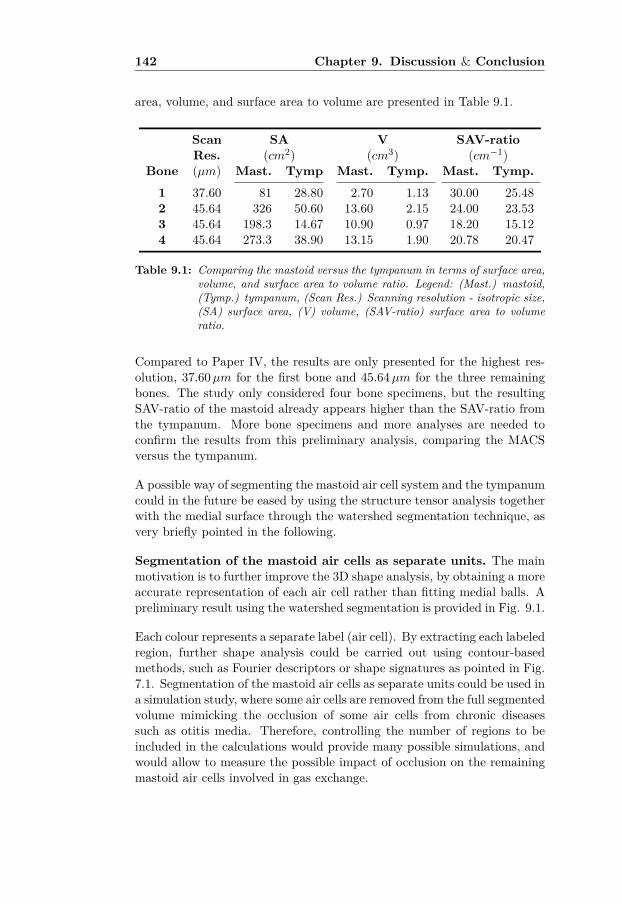
142 Chapter 9. Discussion & Conclusion
area, volume, and surface area to volume are presented in Table 9.1.
Scan SA V SAV-ratioRes. (cm2) (cm3) (cm−1)
Bone (µm) Mast. Tymp Mast. Tymp. Mast. Tymp.
1 37.60 81 28.80 2.70 1.13 30.00 25.482 45.64 326 50.60 13.60 2.15 24.00 23.533 45.64 198.3 14.67 10.90 0.97 18.20 15.124 45.64 273.3 38.90 13.15 1.90 20.78 20.47
Table 9.1: Comparing the mastoid versus the tympanum in terms of surface area,volume, and surface area to volume ratio. Legend: (Mast.) mastoid,(Tymp.) tympanum, (Scan Res.) Scanning resolution - isotropic size,(SA) surface area, (V) volume, (SAV-ratio) surface area to volumeratio.
Compared to Paper IV, the results are only presented for the highest res-olution, 37.60µm for the first bone and 45.64µm for the three remainingbones. The study only considered four bone specimens, but the resultingSAV-ratio of the mastoid already appears higher than the SAV-ratio fromthe tympanum. More bone specimens and more analyses are needed toconfirm the results from this preliminary analysis, comparing the MACSversus the tympanum.
A possible way of segmenting the mastoid air cell system and the tympanumcould in the future be eased by using the structure tensor analysis togetherwith the medial surface through the watershed segmentation technique, asvery briefly pointed in the following.
Segmentation of the mastoid air cells as separate units. The mainmotivation is to further improve the 3D shape analysis, by obtaining a moreaccurate representation of each air cell rather than fitting medial balls. Apreliminary result using the watershed segmentation is provided in Fig. 9.1.
Each colour represents a separate label (air cell). By extracting each labeledregion, further shape analysis could be carried out using contour-basedmethods, such as Fourier descriptors or shape signatures as pointed in Fig.7.1. Segmentation of the mastoid air cells as separate units could be used ina simulation study, where some air cells are removed from the full segmentedvolume mimicking the occlusion of some air cells from chronic diseasessuch as otitis media. Therefore, controlling the number of regions to beincluded in the calculations would provide many possible simulations, andwould allow to measure the possible impact of occlusion on the remainingmastoid air cells involved in gas exchange.

9.2 Future methodological aspects to consider 143
Figure 9.1: Preliminary study on a watershed segmentation of the airspaces com-posing a temporal bone. Each colour represents an air cell.
9.2.2 Technical aspects
This section highlights technical parts that would be interesting to investi-gate in the future.
Further work on the cluster analysis. As illustrated in Fig. 7.3,narrow conduits may block some underneath air cells, it may therefore be ofinterest to further investigate how each location-based cluster is structured,see Fig. 9.2. Indeed, by further studying the distance of each size-basedclustered medial ball to the centroid within each location-based cluster,metrics could be extracted revealing how the medial balls of different sizeare located in relation to each others; e.g. going from very large medialballs towards very small medial balls as in Fig. 9.2(a), or simply in anunstructured manner as in Fig. 9.2(b) suggesting narrow conduits andpossible occlusion for small cells.
Watershed segmentation of the cells. As introduced in the previoussection, a watershed segmentation of the airspace would possibly be a greataddition to the tools used for both a more advanced 3D shape analysisand for a simulation of occlusion of air cells that could happen due to amucosal inflammation. Watershed segmentation is a mature technique andwhich is used in many applications. More information about Watershedsegmentation can be found in [52, 60, 73].

144 Chapter 9. Discussion & Conclusion
Figure 9.2: Future analysis of the intra-location-based clusters for two differenttypes of clusters: (a) structured, and (b) unstructured. The medialballs in (a) are following a certain order in appearance with largerballs close to the centroid and smaller medial balls at the outskirt.The medial balls in (b) are placed in a more random manner wherefor each size-class, the distance from the centroid varies a lot respec-tively.
Multi-scale integration. Only a singular scale was used during the im-plementation of the structure tensor analysis. The filters were only opti-mized for a specific center frequency, a multi-scale implementation couldfurther help the determination of the Euclidean distance transform, wherea binary input volume is needed. Instead of applying a classical thresh-olding on the original data, a multi-scale representation of the norm of thestructure tensor analysis could be used for the thresholding, followed by theEuclidean distance transform. Multi-scale integration could also be used incombination with downsampling of the original data.
From the previous paragraph, a multi-scale integration of the norm of thestructure tensor can be seen as a tensor certainty.
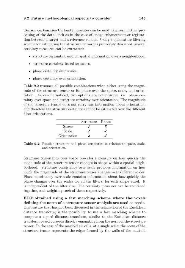
9.2 Future methodological aspects to consider 145
Tensor certainties Certainty measures can be used to govern further pro-cessing of the data, such as in the case of image enhancement or registra-tion between a target and a reference volume. Using a quadrature filteringscheme for estimating the structure tensor, as previously described, severalcertainty measures can be extracted:
• structure certainty based on spatial information over a neighborhood,
• structure certainty based on scales,
• phase certainty over scales,
• phase certainty over orientation.
Table 9.2 resumes all possible combinations when either using the magni-tude of the structure tensor or its phase over the space, scale, and orien-tation. As can be noticed, two options are not possible, i.e. phase cer-tainty over space and structure certainty over orientation. The magnitudeof the structure tensor does not carry any information about orientation,and therefore the structure certainty cannot be estimated over the differentfilter orientations.
Structure PhaseSpace 3 7
Scale 3 3
Orientation 7 3
Table 9.2: Possible structure and phase certainties in relation to space, scale,and orientation.
Structure consistency over space provides a measure on how quickly themagnitude of the structure tensor changes in shape within a spatial neigh-borhood. Structure consistency over scale provides information on howmuch the magnitude of the structure tensor changes over different scales.Phase consistency over scale contains information about how quickly thephase changes over the scales for all the filters, for each single voxel. Itis independent of the filter size. The certainty measures can be combinedtogether, and weighting each of them respectively.
EDT obtained using a fast marching scheme where the voxelsdefining the norm of a structure tensor analysis are used as seeds.One feature that has not been discussed in the estimation of the Euclideandistance transform, is the possibility to use a fast marching scheme tocompute a signed distance transform, similar to the Euclidean distancetransform based on seeds directly emanating from the norm of the structuretensor. In the case of the mastoid air cells, at a single scale, the norm of thestructure tensor represents the edges formed by the walls of the mastoid

146 Chapter 9. Discussion & Conclusion
air cells with a certain thickness. When considering all the points from allthe edges as seeds, a speed volume made of ones can be created, which afast marching scheme can be applied on using the seeds. After a certainnumber of iterations, the resulting volume forms a distance-based volumesimilar to the Euclidean distance transform.
The tensor certainties from the previous discussion topic can then be usedas a mask, to preserve the equivalent Euclidean distance transform corre-sponding to the mastoid air cells while excluding the remaining part. Thisline of work has been briefly tested and appeared to work as it should, butmore work is needed to assess its quality. But, if the hypothesis is correct,there is no need to perform a binary thresholding for estimating the Eu-clidean distance transform in this line of work. The fast marching schemeused to perform this preliminary analysis is based on an implementationfurther detailed in [31].
Improve the medial axis equation. Eq. 7.6 is one possible way ofextracting the medial axis, but not the only one. The main idea behindEq. 7.6 was to increase the flexibility, by keeping a certain amount ofplanar and isotropic parts from the medial surface. As discussed, in Chap-ter 7, several criterions need to be respected in order to be defined as avalid skeleton: homotopy, invariance, thinness, centeredness, smoothness,detail resolution, regularization and level of details, reconstructability, andcomputational scalability.
These criteria are explained in [82]. For the current implementation, thelast two features are not so important, since there is no interest in recon-structing the original shape from the medial balls, and the computationalscalability related to computation power was not a critical point. How-ever, while the Skeleton3D used for comparison was taking a long time,easily above an hour for a complete bone, the medial axis extraction forthe complete bone took about five minutes. More interestingly, the homo-topy of the medial axis, in the current implementation, seemed to be morerepresentative of the shape formed by the mastoid air cell system. Theinvariance of the medial axis current scheme is clearly invariant to scaling,rotation and translation of the original data, since it is extracted from theEuclidean distance transform. Thinness is probably the more critical partof the current implementation, since planar and isotropic parts of the me-dial surface are kept along the medial axis to provide a more continuousrepresentation. However, skeletons extracted from thinning often result inlocations with multiple voxels representing a junction. Nevertheless, morework needs to be done to investigate how thin the current scheme can be-come. The centeredness is guaranteed by the Euclidean distance transform,and by ensuring that not too much noise hampers the borders of the aircell representation.

9.2 Future methodological aspects to consider 147
A qualitative observation of the current medial axis algorithm indicatesa rather good smoothness but no metric was used to investigate on howsmooth the medial axis is. As for the detail resolution, the medial axisalgorithm implemented in this study seems to have a better topology thanthe skeleton obtained using the Skeleton3D module from MeVisLab, asfurther pointed out in Fig. 5.5 by the yellow stars. In terms of regularizationand level of details, it should be noted that the current implementation isstill at an experimental phase, and more work on Eq. 7.6 needs to bedone to ensure a certain robustness in terms sensitivity and to compare theresults with other techniques reviewed in [82].
Propose a conformal mapping. Another line of work is to consider acomplimentary shape analysis that is more based on the surface represent-ing the outer surface of the mastoid air cell system, as the one illustratedin Fig. 5.1. A potential idea is to apply a spherical conformal mappingtransforming the original mesh illustrated in Fig. 5.1 into a unit sphere,where high and low concentration would locally form features. Once thespherical mapping is achieved, a rectangular mapping can be applied, mak-ing it easier to see any patterns on the mesh. Repeating the same principleover several temporal bone specimens would allow comparison of commonpatterns, and would also allow a statistical shape analysis. Similar workhas previously been performed for the brain [51, 70].
Simulate the pneumatization through diffusion. A possible extensionof this work would be to use the work from Zollikofer et al. [94]. Intheir study, bone pneumatization is simulated through a combination ofa Laplace growth model and a Poisson growth model, where the Laplacegrowth model is used to mimic the invasion of mucous epithelial tissuewhile the Poisson growth model mimics the formation of air-filled spaceswithin a growing bone. Applying their method on the micro-CT scans mayimprove our understanding of the pneumatization process by placing a seed(reference point) at the level of the attic (in the tympanum) and letting themodel grow up until it fills all the mastoid air cells.
Perform image registration between several bone specimens. Toallow comparison between different temporal bone specimens, knowing thatthe mastoid air cell system can vary tremendously in shape, image regis-tration needs to be done. As briefly introduced in [23], image registrationcan be defined as the process of mapping input images with a referenceimage. Indeed, when the number of bone specimens available is low (<10),a permutation approach can be used where image registration between twotemporal bone specimens is performed many times. By investigating whichpermutation that provides the smoothest displacement fields, it is possibleto use the resulting temporal bone as a template to which the remainingtemporal bone specimens can be registered. When the number of tempo-

148 Chapter 9. Discussion & Conclusion
ral bones is larger, a possible solution is to select one temporal bone as areference volume, then register all the remaining temporal bone specimensto that reference, calculate an average over all registered temporal bonespecimens, which then becomes the template, and register each temporalbone specimen to that template (including the one used for the reference).Due to the large amount of data imposed by the micro-CT scanning, imageregistration can be done through the graphical processing unit (GPU) asfurther detailed in [22].
Before concluding, besides the discovery of the micro-channels, some addi-tional unreported findings are presented. They deserve some attention asthey may provide more information about the possible roles of the mastoidin the temporal bone. First strands were found deep inside the mastoid aircell system. Second, pores along the bony septae were commonly observed.Also, spicules protruding from the walls of the mastoid air cells has alsoraised the attention by their consistent findings. A section is dedicated toeach of these unreported findings and possible roles are suggested thoughfurther research is needed.
9.3 Strands and membranes within the MACS
Figure 9.3: Mucosal strands isolating the central air cell from the surroundingones. Source: Temporal Bone Histology Lab, Otorhinolaryngology,University Zurich (permission granted by Prof. Dr. Med. AlexanderHuber).
Originally believed to originate from the fact that the bone specimens aredried, the mucosa normally lining the air cells was thought to be looseand form strands barely visible on the micro-CT scans. However, whencarefully observing these strands, either on 2D slices and even better in

9.3 Strands and membranes within the MACS 149
3D while using volume rendering, these epithelial strands have well definedpyramidal bases at their attachment locations. These structures, thoughvery thin, have only been reported in the tympanum between the tympanicwalls and the ossicles, known as the mucosal folds. Within the mastoid aircells, to the author’s knowledge, this feature has never been illustrated in3D in the literature so far.
This finding is recurrent and has been observed in almost all specimensavailable for scanning. Fig. 9.3 illustrates the presence of two strands clos-ing the openings between bony septae in the MACS from a histologicalsection, highlighted by the two yellow rectangles. In this histological sec-tion, the central air cell becomes isolated from the surrounding air cells.A positive aspect of these strands is that they further increase the surfacearea to volume ratio, especially if the inflammation is only temporary. In-terestingly, it is possible to observe these strands using micro-CT scans.Fig. 9.4 illustrates the presence of strands found in the apical air cells ofthe mastoid pointed by arrows.
Figure 9.4: Strands (pointed by arrows) together with membranes separatingsome air cells at the apex of the mastoid.
The top three arrows show differences in structure: the top left yellow arrowshows a full membrane, while the top right yellow illustrates a standardstrand. The bottom red arrow points towards a strand possibly containinga structure along its path. The two remaining yellow arrows point to moremembraneous strand types as the top left arrow, proving that such strandscan also exist further lateral in the mastoid air cell system.
In Fig. 9.5, multiple strands can be observed at the level of the aditus adantrum towards the midline of the mastoid air cell system and pointed by

150 Chapter 9. Discussion & Conclusion
yellow arrows. Interestingly, at the intersection between multiple strands, atriangular patch of mucosa is visible. The yellow circle particularly pointsout a strand having a local increase in its thickness, possibly indicating thepresence of a Pacinian corpuscle attached to it.
Figure 9.5: Multiple strands from at the level of the antrum highlighted by theyellow arrows. Notice the pyramidal node at the intersection pointedby the yellow stars (scan resolution 38 µm).
Another interesting observation is the presence of small holes carved intothe septae separating the air cells, as further detailed in the next section.
9.4 Pores in the septae
Pores located within the mastoid air cell system in human temporal boneshave not, to the author’s knowledge, been reported before. Fig. 9.6 il-lustrates the presence of many pores in the bone septae, highlighted withthe white stars. The origin and function of these ventilation pores is notunderstood. Plates in trabecular plates found in long bones, such as thefemur, also contain openings similar to the pores found in this study.
In terms of physiology, when trying to find an analogy with the lungs, thepore of Kohn comes in mind. A Kohn pore is a tiny opening in the alveoli,allowing communicating between two adjacent alveoli. The main purposeof this shunt is to allow oxygen to reach alveoli which are isolated at thelevel of the alveolar ducts or higher up in the respiratory trunk or when thelungs are temporally collapsed. However, while the lungs can collapse, themastoid air cell system is fixed in structure by the bone septae separatingthe air cells. The soft epithelial lining is not well represented in X-raymicro-CT, if at all, making it impossible at this level to understand their

9.4 Pores in the septae 151
Figure 9.6: Ventilation pores in the mastoid air cell system. For better localiza-tion in the temporal bone, part of the ossicular chain is shown on thetop of this coronal view showing the lower half of the mastoid bone,with the semi-circular canals at the top left. The white stars pointout few of the ventilation pores.
role. Some of the small pores might be fully covered by mucosa.
It is, however, believed that some pores may be too large to be fully cov-ered by mucosa, and therefore still allow air to pass through them even ifcovered by mucosa. Moreover, these bone specimens are from corpses andwere fixated. Therefore, the mucosa lining the walls of the mastoid air cellsis no longer nourished by blood, and is no longer playing its role in pressureregulation. When in the presence of blood, the mucosa lining these poresmay expand up to a point where the pore becomes temporally occluded,and open again when the mucosa shrinks in thickness. A mechanism ofopening-closing of these pores could be possible. Interestingly, some porescan be found at the attic of the tympanum right at the level of the antrumnear the posterior level of the malleus head, see Fig.9.7.

152 Chapter 9. Discussion & Conclusion
Figure 9.7: Pores found at the level of the epitympanum right above the ossicles.
Another observed feature is the presence of spicules in some air cells.
9.5 Bone spicules
These bone spicules are believed to be the remnants of an early stage ofthe mastoid process formation during infancy. As described in Chapter 3,the mastoid is more of a flat bone as the remaining cranial bones, whichcontent is mostly primitive bone marrow. After the primitive bone marrowbeing converted into loose mesenchyme tissue, the epithelial layer coveringthe tympanum is invading the trabecular space. It is personally believedthat this internal pressure, along with the growth of the skull bones as wellas the strengthening of the sternomastoid muscle, leads to a breakage ofsome of the trabecular rods and plates. After an certain age in the infancy,around 7-8 years of age with some exceptions, this process stops and theair cells are considered fully formed. The broken trabecular rods and platesthen become spicules as visible in some air cells. It should be noted thatosteoneogenesis, formation of new bone, is also occurring during chronicmiddle ear infection as pointed by [12]. Such bone formation could resultin the appearance of spicule pointing normal to the bone septae, as alsoillustrated in [75].
Fig. 9.8, in four steps, resumes this process, where the epithelial mu-

9.5 Bone spicules 153
Figure 9.8: Formation of the spicules at the early stages of the mastoid forma-tion. Legend: (1) Classical organization of a bone with trabecularrods forming trabecular spaces, filled with bone marrow between twocortical bone layers. In (2), the rods are rupturing due to multiplesources: muscle pulling the bone downward, epithelial layer pushedby air coming from the forming tympanum. In (3), the tip of the rup-tures rods slowly erode, giving the appearance of smooth spikes. In(4), the mucosa and epithelial lining cover all the walls and spiculesof the mastoid air cell system.
cosa lining the forming tympanum invades the mastoid bone. During thisprocess, some of the trabecular rods and plates slowly split through boneresorption via the osteoblast-osteoclast interaction. It is possible that thisprocess stabilises at eight years of age and hence the presence of spiculesor incomplete plates within some of the mastoid air cells. In Fig. 9.8(1),a very simplistic representation of the mastoid bone with some trabeculaeand bone marrow before the invasion of the epithelial mucosa is given. InFig. 9.8(2), the epithelial mucosa has started to penetrate the cancellouspart of the bone, with some bone resorption of some of the trabecular rodsand plates illustrated. In Fig. 9.8(3), the epithelial lining takes more andmore spaces, and the broken rods present a more spicule like shape. In Fig.9.8(4), the epithelial lining is fully covering all the bone inner surface. Atthis stage, the mastoid bone is fully pneumatized. A volume rendering ofthe spicules using micro-CT, highlighted by yellow stars and covered withmucosa, is provided in Fig. 9.9. As explained earlier, the spicules are oftenthe supports for mucosal strands, as pointed by the multiple arrows for thespicule located to the outmost right emphasized with the right yellow star.
Though cats have a bulla instead of a mastoid as in humans, Sula et al.[75] reported the occasional formation of irregular bony spicules in cats

154 Chapter 9. Discussion & Conclusion
Figure 9.9: Spicules covered by mucosa and strands, respectively marked withyellow stars and arrows.
with a history of chronically affected ears . Per Cayé-Thomasen et al. [11]reported the formation of bone in the presence of a pathological bone, suchas in chronic otitis media. To investigate whether the bony spicules resultfrom the original bone formation, or from a remodelling due to chronicpathology, more clinical work needs to be done and is beyond the scope ofthis work.
9.6 Conclusion
The content of this thesis was not aimed at being groundbreaking froma technological point of view, and does not intend to contradict previousmethods used in the field of ENT, especially when measuring geometri-cal properties of the mastoid air cell system in human temporal bone viamicro-CT scans. The overall main goal of this PhD was to open bridgesbetween two fascinating worlds: the mastoid air cell system and advancedimage processing tools, allowing to extract more information than the soleextraction of surface area and volume. Flexibility of the algorithm, whilepreserving a certain robustness of the methods, was considered as a higherpriority when selecting the image processing tools. The flexibility allowedtuning the different algorithms based on the anatomical structures, whilerobustness was important to preserve consistency over the different studies.Through the thesis, visualization has been a very important tool. Indeed,

9.6 Conclusion 155
the complexity imposed by the mastoid air cell system implies a constantverification of any obtained result. The importance of visualization in thisstudy has also shaped some of the scientific contributions to be more quali-tative than quantitative. Another good reason for this choice is the fact thatso little is known about the geometrical properties of the mastoid air cellsystem that there is a need to be acquainted with its intricate structures.


Bibliography
[1] Illustration of the eustachian tube at the level of nasopharynx.http://upload.wikimedia.org/wikipedia/commons/e/e3/Gray855.png.
[2] A.Ilea, A. Butnaru, S. Sfrângeu, M. Hedeşiu, C. Dudescu, P. Berce,H. Chezan, L. Hurubeanu, V. Trombiţaş, R. Câmpian, and S. Albu. Roleof mastoid pneumatization in temporal bone fractures. American Journal ofNeuroradiology, 35(7):1398–1404, 2014.
[3] A. Allam. Pneumatization of the temporal bone. Ann. Otol. Rhinol. Laryn-gol., 78:48–64, 1969.
[4] B. Anson, J. Wilson, and J. Gaardsmoe. Air cells of petrous portion oftemporal bone in a child four and a half years old: A study based on waxplate reconstructions. Archives of Otolaryngology, 27(5):588–605, 1938.
[5] B. Ars and N. Ars-Piret. Middle ear pressure balance under normal condi-tions. specific role of the middle ear structure. Acta Otorhinolaryngol. Belg.,48:339–342, 1994.
[6] B. Ars, F. Wuyts, P. V. de Heyning, I. Miled, J. Bogers, and E. V. Marck.Histomorphometric study of the normal middle ear mucosa. Acta Otolaryngol.(Stockh), 117:704–707, 2006.
[7] M. Berg, O. Cheong, M. Kreveld, and M. Overmars. Computational Geome-try: Algorithms and Applications. Springer-Verlag TELOS, Santa Clara, CA,USA, 3rd ed. edition, 2008. ISBN 9783540779735.
[8] S. Biasotti, B. Falcidieno, D. Giorgi, and M. Spagnuolo. MathematicalTools for Shape Analysis and Description. Synthesis Lectures on Com-puter Graphics and Animation. Morgan & Claypool Publishers, 2014. ISBN9781627053631.
[9] H. Blum. A Transformation for Extracting New Descriptors of Shape. Modelsfor the Perception of Speech and Visual Form, Cambridge, MIT Press, pages362–380, 1967.
[10] T. Caliński and J. Harabasz. A dendrite method for cluster analysis. Com-munications in Statistics, 3(1):1–27, 1974.
[11] P. Cayé-Thomasen, A. Hermansson, and M. T. K. Prellner. Pathogenesis ofmiddle ear adhesions. The Laryngoscope, 106(4):463–469, 1996.
[12] P. Cayé-Thomasen, A. Hermansson, M. Tos, and K. Prellner. Bone modelingdynamics in acute otitis media. The Laryngoscope, 109(5):723–729, 1999.
[13] O. Cros. Image analysis and visualization of the human mastoid air cell sys-tem. Licentiate thesis 1730, Linköping University, Department of BiomedicalEngineering, 2015.
[14] O. Cros, A. Eklund, M. Gaihede, and H. Knutsson. Local size descriptor ofmastoid air cells in human temporal bone based on a structure tensor analysis
158 BIBLIOGRAPHY
from an euclidean distance transform. Computerized Medical Imaging andGraphics. Submitted.
[15] O. Cros, A. Eklund, M. Gaihede, and H. Knutsson. Enhancement of microchannels within the human mastoid bone based on local structure tensor anal-ysis. IEEE The sixth International Conference on Image Processing Theory,Tools and Applications (IPTA16). 2016. In Press.
[16] O. Cros, A. Eklund, M. Gaihede, and H. Knutsson. Surface and curve skele-ton from a structure tensor analysis applied on mastoid air cel ls in humantemporal bones. 2017 IEEE 12th International Symposium on BiomedicalImaging (ISBI), 2017.
[17] Z. Csákányi, G. Katona, E. Josavai, F. Mohos, and I. Sziklai. Volume andsurface of the mastoid cell system in otitis media with effusion in children:a case-control study by three-dimensional reconstruction of computed tomo-graphic images. Otology And Neurotology, 32:64–70, 2011.
[18] W. Doyle. Increases in middle ear pressure resulting from counter-diffusion ofoxygen and carbon dioxide into the middle ear of monkeys. Acta Otolaryngol.,117(5):708–713, 1997.
[19] W. Doyle. Mucosal surface area determines the middle ear pressure responsefollowing establishment of sniff-induced underpressures. Acta Otolaryngol.,119(6):695–702, 1999.
[20] R. Drebin, L. Carpenter, and P. Hanrahan. Volume rendering. ComputerGraphics, 22(4):65–74, 1988.
[21] A. Eklund, M. Andersson, and H. Knutsson. True 4D image denoising on theGPU. International Journal of Biomedical Imaging, 2011:1–16, 2011.
[22] A. Eklund, P. Dufort, D. Forsberg, and S. LaConte. Medical image processingon the GPU - Past, present and future. Medical Image Analysis, 17(8):1073–1094, 2013.
[23] F. E. A. El-Gamal, M. Elmogy, and A. Atwan. Current trends in medicalimage registration and fusion. Egyptian Informatics Journal, 17(1):99 – 124,2016.
[24] J. Fehrenbach and J.-M. Mirebeau. Sparse Non-negative Stencils forAnisotropic Diffusion. Journal of Mathematical Imaging and Vision,49(1):123–147, 2014.
[25] R. C. Gonzalez, R. E. Woods, and S. L. Eddins. Digital Image Processingusing MATLAB. Pearson Prentice Hall, 2004. ISBN 0130085197.
[26] G. Granlund and H. Knutsson. Signal Processing for Computer Vision.Kluwer Academic Publishers, 1995. ISBN 0792395301.
[27] H. Gray and H. Carter. Gray’s Anatomy (Illustrated With 1247 ColouredWell Drawing Engrawings). eKitap Projesi, 2016. ISBN 9786059654708.
[28] M. Gurcan, L. Boucheron, A. Can, A. Madabhushi, N. Rajpoot, and B. Yener.Histopathological image analysis: A review. IEEE reviews in biomedicalengineering, 2:147–171, 2009.
[29] L. Haglund. Adaptive Multidimensional Filtering. Linköping Studies in Sci-ence and Technology. Dissertations No. 284, Linköping University, Sweden,1992.

BIBLIOGRAPHY 159
[30] S.-J. Han, M. Song, J. Kim, W.-S. Lee, and H.-K. Lee. Classification oftemporal bone pneumatization based on sigmoid sinus using computed to-mography. Clinical Radiology, 62(11):1110–1118, 2007.
[31] M. S. Hassouna and A. A. Farag. Multistencils fast marching methods: Ahighly accurate solution to the eikonal equation on cartesian domains. IEEETransactions on Pattern Analysis and Machine Intelligence, 29(9):1563–1574,2007.
[32] E. Hentzer. Histological studies of the normal mucosa in the middle ear,mastoid cavities and eustachian tube. Annals of Otology, Rhinology andLaryngology, 79:825–833, 1970.
[33] W. H. Hesselink and J. B. T. M. Roerdink. Euclidean skeletons of digital im-age and volume data in linear time by the integer medial axis transform. IEEETransactions on Pattern Analysis and Machine Intelligence, 30(12):2204 –2217, 2008.
[34] C. Hodez, C. Griffaton-Taillandier, and I. Bensimon. Cone-beam imaging:Applications in ENT. European Annals of Otorhinolaryngology, Head andNeck Diseases, 128(2):65–78, 2011.
[35] C. T. Huang and O. R. Mitchell. Rapid euclidean distance transform usinggrayscale morphology decomposition. In IEEE Computer Society Conferenceon Computer Vision and Pattern Recognition, pages 695–697, 1991.
[36] N. Ikonomatakis, K. Plataniotis, M. Zervakis, and A. Venetsanopoulos. Re-gion growing and region merging image segmentation. In 13th InternationalConference on Digital Signal Processing Proceedings, volume 1, pages 299–302, 1997.
[37] M. Isono, K. Murata, H. Azuma, M. Ishikawa, and A. Ito. Computerizedassessment of the mastoid air cell system. Auris Nasus Larynx, 26(2):139–145, 1999.
[38] B. Jähne. Digital Image Processing. 5th revised and extended edition. 2002.ISBN 3540677542.
[39] P. Jensen and M. Gaihede. Congestion of mastoid mucosa and influence onmiddle ear pressure - Effect of retroauricular injection of adrenaline. HearingResearch Special Issue MEMRO, 340:121–126, 2016.
[40] M. K. Kalra, M. M. Maher, T. L. Toth, B. Schmidt, B. L. Westerman, H. T.Morgan, and S. Saini. Techniques and applications of automatic tube currentmodulation for CT. Radiology, 233(3):649–657, 2004.
[41] D. G. Kendall. The diffusion of shape. Advances in Applied Probability,9(3):428–430, 1977.
[42] M. Kerschnitzki, P. Kollmannsberger, M. Burghammer, G. Duda,R. Weinkamer, W. Wagermaier, and P. Fratzl. Architecture of the osteo-cyte network correlates with bone material quality. Journal of Bone andMineral Research, 28(8):1837–1845, 2013.
[43] H. Knutsson. Filtering and Reconstruction in Image Processing. PhD thesis,Linköping University, 1982.
[44] H. Knutsson, M. Andersson, and J. Wiklund. Advanced filter design. InScandinavian conference on image analysis (SCIA), 1999.
[45] H. Knutsson and M. T. Andersson. Optimization of sequential filters. In InProceedings of the SSAB Symposium on Image Analysis, pages 87–90, 1995.

160 BIBLIOGRAPHY
[46] A. Koç, G. Ekinci, A. Bilgili, I. Akpinar, H. Yakut, and T. Han. Evalua-tion of the mastoid air cell system by high resolution computed tomography:three-dimensional multiplanar volume rendering technique. J. Laryngol Otol.,117(8):595–5988, 2003.
[47] G. Läthén. Level Set Segmentation and Volume Visualization of VascularTrees. PhD thesis, 2013. ISBN 03457524.
[48] D. Lee, B. Jun, D. Kim, M. Jung, and S. Yeo. Volume variation of mas-toid pneumatization in different age groups: a study by three-dimensionalreconstruction based on computed tomography images. Surg Radiol Anat,27:37–42, 2005.
[49] L. T.-C. Lee, L. Rangasami, and C. Chong-Nam. Building skeleton modelsvia 3-d medial surface/axis thinning algorithms. Computer Vision, Graphics,and Image Processing, 56(6):462–478, 1994.
[50] T. Lee, R. Kashyap, and C. Chu. Building skeleton models via 3-d medialsurface axis thinning algorithms. In CVGIP: Graphical Models and ImageProcessing, volume 56, pages 462–478, 1994.
[51] J. Lefèvre and G. Auzias. Spherical Parameterization for Genus Zero Surfacesusing Laplace-Beltrami Eigenfunctions. Proceedings Geometric Science ofInformation: Second International Conference, GSI 2015, Palaiseau, France,F. Nielsen and F. Barbaresco, Springer International Publishing, pages 121–129, 2015.
[52] D. Legland, I. Arganda-Carreras, and P. Andrey. MorphoLibJ: integratedlibrary and plugins for mathematical morphology with ImageJ. Bioinformat-ics, 32(22):3532, 2016.
[53] W. E. Lorensen and H. E. Cline. Marching cubes: A high resolution 3Dsurface construction algorithm. ACM Computer Graphics, 21:163–169, 1987.
[54] M. Luntz, S. Malatskey, M. Tan, E. Bar-Meir, and D. R. D. Volume ofmastoid pneumatization: three-dimensional reconstruction with ultrahigh-resolution computed tomography. Ann Otol Rhinol Laryngol, 110 (5Pt1):486–490, 2001.
[55] A. Maier, L. Wigstrom, H. Hofmann, J. Hornegger, L. Zhu, N. Strobel, andR. Fahrig. Three-dimensional anisotropic adaptive filtering of projection datafor noise reduction in cone beam CT. Med Phys., 38(11):5896–5909, 2011.
[56] B. Masschaele, V. Cnudde, M. Dierick, P. Jacobs, L. V. Hoorebeke, andJ. Vlassenbroeck. UGCT: New x-ray radiography and tomography facility.Nucl. Instrum. Meth., A580:266–269, 2007.
[57] B. Masschaele, M. Dierick, D. V. Loo, V. Cnudde, M. N. Boone, L. Brabant,E. Pauwels, V. Cnudde, and L. V. Hoorebeke. HECTOR: A 240kv micro-CTsetup optimized for research. Journal of Physics: Conference Series, 463(1):1–4, 2007.
[58] R. Matanda, P. V. D. Heyning, J. Bogers, and B. Ars. Behaviour of middleear cleft mucosa during inflammation: Histo-morphometric study. Acta Oto-Laryngologica, 126:905–909, 2006.
[59] W. W. Mayo-Smith, A. K. Hara, M. Mahesh, D. V. Sahani, and W. Pavlicek.How i do it: Managing radiation dose in CT. Radiology, 273(3):657–672, 2014.
[60] F. Meyer and S. Beucher. Morphological segmentation. Journal of VisualCommunication and Image Representation, 1(1):21 – 46, 1990.

BIBLIOGRAPHY 161
[61] A. Miracle and S. Mukherji. Conebeam ct of the head and neck, part 2:Clinical applications. American Journal of Neuroradiology, 30(7):1285–1292,2009.
[62] M. Miura, H. Takahashi, I. Honjo, S. Hasebe, and M. Tanabe. Influence ofthe gas exchange function through the middle ear mucosa on the developmentof sniff-induced middle ear diseases. The Laryngoscope, 108:683–686, 1998.
[63] I. Nyström, G. S. di Baja, and S. Svensson. Curve Skeletonization by JunctionDetection in Surface Skeletons. In C. Arcelli et al. (Eds): IWVF4 Capri,LNCS 2059, Springer-Verlag Berlin Heidelberg, pages 229–238, 2001.
[64] M. Park, S. Yoo, and D. H. Hoon. Measurement of surface area in the humanmastoid air cell system. J. Laryngol. Otol., 114:93–96, 2000.
[65] S. P. Raman, M. Mahesh, R. V. Blasko, and E. K. Fishman. CT scan pa-rameters and radiation dose: practical advice for radiologists. Journal of theAmerican College of Radiology : JACR, 10(11):840–846, 2013.
[66] J. Sadé and A. Ar. Middle ear and auditory tube: Middle ear clearance, gasexchange, and pressure regulation. Otolaryngol. Head Neck Surg., 116:499–524, 1997.
[67] P. K. Saha, G. Borgefors, and G. S. di Baja. A survey on skeletonizationalgorithms and their applications. Pattern Recognition Letters, 76:3 – 12,2016.
[68] L. Serino and G. S. d. Baja. Pruning the 3d curve skeleton. 2014 22ndInternational Conference on Pattern Recognition, pages 2269–2274, 2014.
[69] M. Sezgin and B. Sankur. Survey over image thresholding techniquesand quantitative performance evaluation. Journal of Electronic Imaging,13(1):146–165, 2007.
[70] Y. Shi, R. Lai, and A. Toga. Conformal mapping via metric optimization withapplication for cortical label fusion. Proceedings of the conference InformationProcessing in Medical Imaging, 23:244–255, 2013.
[71] A. J. Silver, I. Janecka, J. Wazen, S. K. Hilal, and J. N. Rutledge. Compli-cated cholesteatomas: Ct findings in inner ear complications of middle earcholesteatomas. Radiology, 164(1):47–51, 1987.
[72] A. Sobiecki, A. Jalba, and A. Telea. Comparison of curve and surface skele-tonization methods for voxel shapes. Pattern Recognition Letters, 47:147 –156, 2014.
[73] P. Soille and L. Vincent. Determining watersheds in digital pictures via flood-ing simulations. Visual Communications and Image Processing ’90, 1360:240–250, 1990.
[74] J. Stewart. The histopathology of mastoiditis. Proceedings of the RoyalSociety of Medicine, 21(10):1743–1758, 1928.
[75] M. M. Sula, B. L. Njaa, and M. E. Payton. Histologic characterization of thecat middle ear. Veterinary Pathology, 51(5):951–967, 2014.
[76] B. Svensson. A Multidimensional Filtering Framework with Applications toLocal Structure Analysis and Image Enhancement. Linköping Studies in Sci-ence and Technology. Dissertations No. 1171, Linköping University, Sweden,2008.
[77] J. Swarts, B. C. Doyle, C. Alper, and W. Doyle. Surface area-volume re-lationships for the mastoid air cell system and tympanum in adult humans:

162 BIBLIOGRAPHY
Implications for mastoid function. Acta oto-laryngologica, 130(11):1230–1236,2010.
[78] J. Swarts, S. Folay, C. Alper, W. Doyle, and J. William. Mastoid geometryin a cross-section of humans from infancy through early adulthood with aconfirmed history of otitis media. International journal of pediatric otorhi-nolaryngology, 76(1):137–141, 2011.
[79] J. D. Swarts, B. Doyle, C. Alper, and W. Doyle. Surface area-volume re-lationships for the mastoid air cell system and tympanum in adult humans:Implications for mastoid function. Acta Oto-Laryngologica, 130(11):1230–1236, 2011.
[80] J. D. Swarts, B. Doyle, and W. Doyle. Surface area-volume relationships forthe mastoid air cell system in adult humans. The Journal of Laryngology andOtology, 125(6):580–584, 2011.
[81] J. Swartz and L. Loevner. Imaging of the Temporal Bone. Thieme PublishersSeries, 2011. ISBN 9781588906496.
[82] A. Tagliasacchi, T. Delame, M. Spagnuolo, N. Amenta, and A. Telea. 3dskeletons: A state-of-the-art report. Computer Graphics Forum, 35(2):573 –597, 2016.
[83] A. Telser, J. Young, and K. Baldwin. Elsevier’s Integrated Histology. Mos-by/Elsevier. Inc. Philadelphia, 2007. ISBN 0323033881.
[84] N. Todd, R. Pitts, I. Braun, and H. Heindel. Mastoid size determinedwith lateral radiographs and computerized tomography. Acta Otolaryngolica,103:226–231, 1987.
[85] M. Tos. Manual of Middle Ear Surgery. Vol.2: Mastoid Surgery and Recon-structive Procedures. Georg Thieme Verlag, 1995. ISBN 0865775893.
[86] C. Virapongse, M. Sarwar, S. Bhimani, C. Sasaki, and R. Shapiro. Computedtomography of temporal bone pneumatization: 1. Normal pattern and mor-phology. In American Journal of Roentgenology, volume 145, pages 473–481.1985.
[87] J. Vlassenbroeck, M. D. B. Masschaele, V. Cnudde, L. V. Hoorebeke, andP. Jacobs. Software tools for quantification of x-ray microtomography at theUGCT. Nuclear Instruments and Methods in Physics Research, A(580):442–445, 2007.
[88] J. Vrabec, S. Champion, J. G. R. Johnson, and G. Chaljub. 3D CT 534imaging method for measuring temporal bone aeration. Acta Otolaryngol,122:831–835, 2002.
[89] H. Wang, C. Northrop, B. Burgess, M. Liberman, and S. Merchant. Three-dimensional virtual model of the human temporal bone: A stand-alone, down-loadable teaching tool. Otology and neurotology: official publication of theAmerican Otological Society, American Neurotology Society and EuropeanAcademy of Otology and Neurotology, 27(4):452–457, 2006.
[90] J. Wu. Advances in K-means Clustering: A Data Mining Thinking. SpringerPublishing Company, Incorporated, 2012. ISBN 9783642298066.
[91] J. Yi and J. B. Ra. A locally adaptive region growing algorithm for vascularsegmentation. Int. J. Imaging Systems and Technology, 13:208–214, 2003.
[92] D. Zhang and G. Lu. Review of shape representation and description tech-niques. 37:1–19, 2004.

BIBLIOGRAPHY 163
[93] J. Zhang, C.-H. Yan, C.-K. Chui, and S.-H. Ong. Fast segmentation of bonein CT images using 3d adaptive thresholding. Computers in Biology andMedicine, 40(2):231–236, 2010.
[94] C. Zollikofer and J. Weissmann. A morphogenetic model of cranial pneuma-tization based on the invasive tissue hypothesis. The Anatomical Record,WILEY-LISS, INC., 291:1446–1454, 2008.

Papers
The articles associated with this thesis have been removed for copyright
reasons. For more details about these see:
http://urn.kb.se/resolve? urn:nbn:se:liu:diva-137288