statistics and quantitative analysis u4320 segment 7 : hypothesis testing prof. sharyn o’halloran

Statistics and Quantitative Analysis U4320

Segment 7 :Hypothesis Testing

Prof. Sharyn O’Halloran

Hypothesis Testing I. Introduction

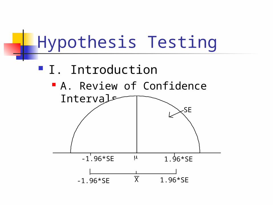
A. Review of Confidence Intervals

SE

-1.96*SE 1.96*SE

-1.96*SE 1.96*SEX

Introduction (cont.)

B. Hypothesis Testing: Basic Definitions 1. A Hypotheses is a statement about the

population 2. Null Hypothesis

The Null Hypothesis (Ho)- the statement about our data that we want to test.

It is always stated as an equality. For instance; Ho: = 82, where is the average test score Or, H0: = 0, where is the difference

between men's and women' salaries is zero.


3. Alternative Hypothesis Every Null Hypothesis has an associated

Alternative Hypothesis, denoted Ha. This is always stated as an inequality either ,

>, or <. For instances, the alternative hypothesis

to the test scores having a mean of 82 might be Ha: 82.

The alternative hypothesis to men's and women's' salaries being equal might be Ha: > 0.


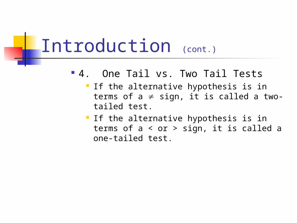
4. One Tail vs. Two Tail Tests If the alternative hypothesis is in terms of a

sign, it is called a two-tailed test. If the alternative hypothesis is in terms of a <

or > sign, it is called a one-tailed test.


C. Three Methods for Testing Hypothesis

1. Method I: Testing hypotheses using confidence intervals.

2. Method II: Testing hypotheses using p-values.

3. Method III: Testing hypotheses using critical values.

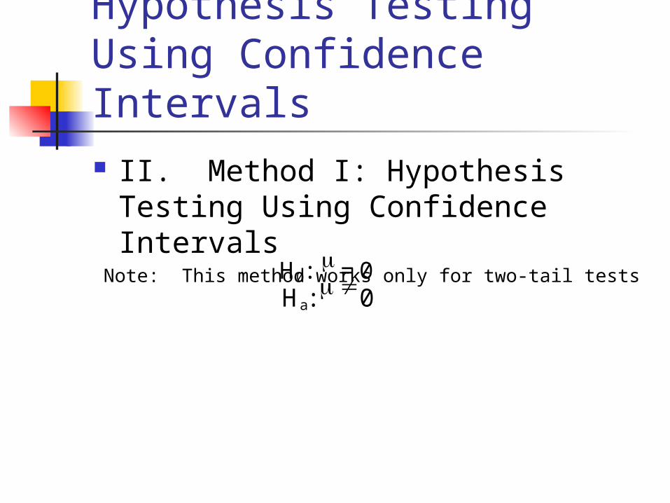
Hypothesis Testing Using Confidence Intervals II. Method I: Hypothesis Testing

Using Confidence Intervals Note: This method works only for two-tail tests

H0: = 0

Ha: 0

Hypothesis Testing Using Confidence Intervals (cont.)

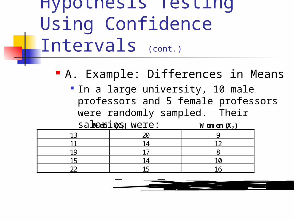
A. Example: Differences in Means In a large university, 10 male professors

and 5 female professors were randomly sampled. Their salaries were:

Men (X1) Women (X2)

13 20 9 11 14 12 19 17 8 15 14 10 22 15 16

X1 = 16 X2 = 11


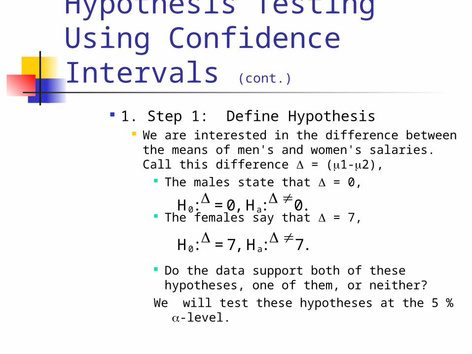
1. Step 1: Define Hypothesis We are interested in the difference between

the means of men's and women's salaries. Call this difference = (1-2),

The males state that = 0, The females say that = 7,

Do the data support both of these hypotheses, one of them, or neither?

We will test these hypotheses at the 5 % -level.

H0: = 0, Ha: 0.

H0: = 7, Ha: 7.


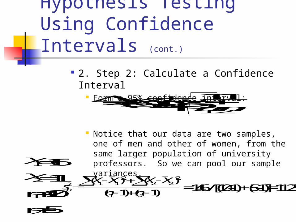
2. Step 2: Calculate a Confidence Interval Form a 95% confidence interval:

Notice that our data are two samples, one of men and other of women, from the same larger population of university professors. So we can pool our sample variances.

= (X1-X2) t.025 * sp * 11

12nn

X1 = 16

X2 = 11

n1 = 10

n2 = 5

sX X X X

n np2 1 1

22 2

2

1 21 1

( ) ( )

( ) ( ) = 146 / [(10-1) + (5-1)]= 11.23


(cont.)

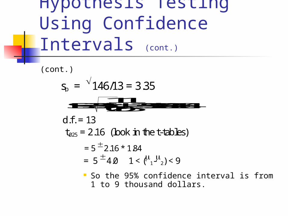
So the 95% confidence interval is from 1 to 9 thousand dollars.

sp = 146/13 = 3.35

SE = 3.35*11015 = 3.35 * .548= 1.84

d.f. = 13

t.025 = 2.16 (look in the t-tables)

= 5 2.16 * 1.84

= 5 4.0 1 < (1-2) < 9


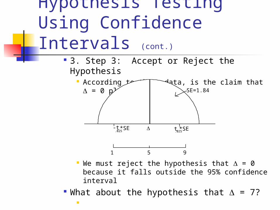
3. Step 3: Accept or Reject the Hypothesis According to these data, is the claim that = 0

plausible?

We must reject the hypothesis that = 0 because it falls outside the 95% confidence interval

What about the hypothesis that = 7?

SE=1.84

1

9

-t.025

*SE t.025

*SE

5

reject

reject

We cannot reject the null hypothesis H0: = 7 at the 5% level.


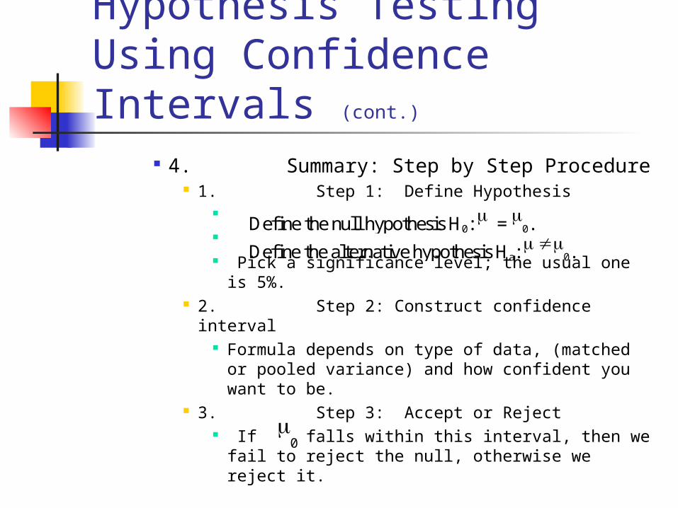
4. Summary: Step by Step Procedure

1. Step 1: Define Hypothesis Pick a significance level; the usual one is 5%.

2. Step 2: Construct confidence interval

Formula depends on type of data, (matched or pooled variance) and how confident you want to be.

3. Step 3: Accept or Reject If falls within this interval, then we fail to

reject the null, otherwise we reject it.

Define the null hypothesis H0: = 0.

Define the alternative hypothesis Ha: 0.

0


B. Another Example: Matched Data A firm producing plate glass has developed a

less expensive tempering process to allow glass for fireplaces to rise to a higher temperature without breaking. To test it, five different plates of glass were drawn randomly from a production run, then cut in half, with one half tempered by the new process and one half tempered by the old. The two halves were then heated until they broke. The results of the experiment look like this: (next slide)


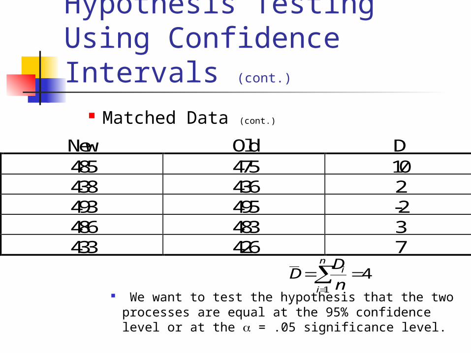
Matched Data (cont.)

We want to test the hypothesis that the two processes are equal at the 95% confidence level or at the = .05 significance level.

New Old D 485 475 10 438 436 2 493 495 -2 486 483 3 433 426 7

DD

ni

i

n

1

4


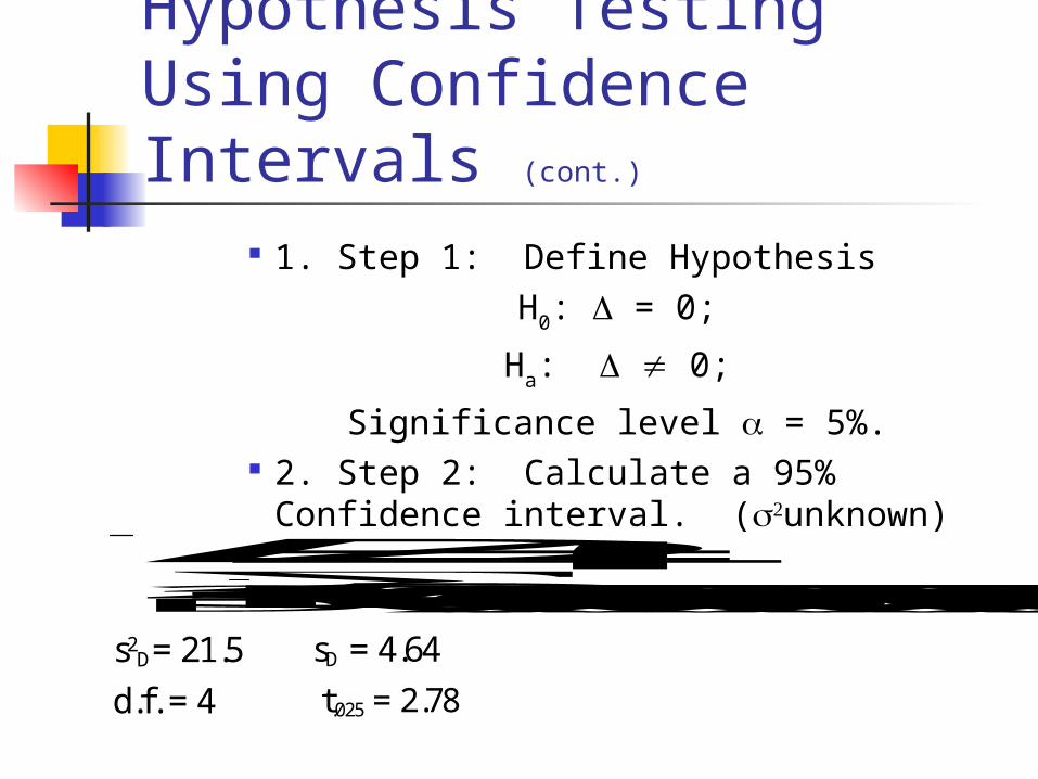
1. Step 1: Define Hypothesis H0: = 0;

Ha: 0;

Significance level = 5%. 2. Step 2: Calculate a 95% Confidence

interval. (unknown) D = 4 s2D= (D-D)2/(n-1) = (10-4)2 + (2-4)2 + (-2-4)2 + (3-4)2 +(7-4)2 / (5-1)

s2D= 21.5 sD = 4.64

d.f. = 4 t.025 = 2.78


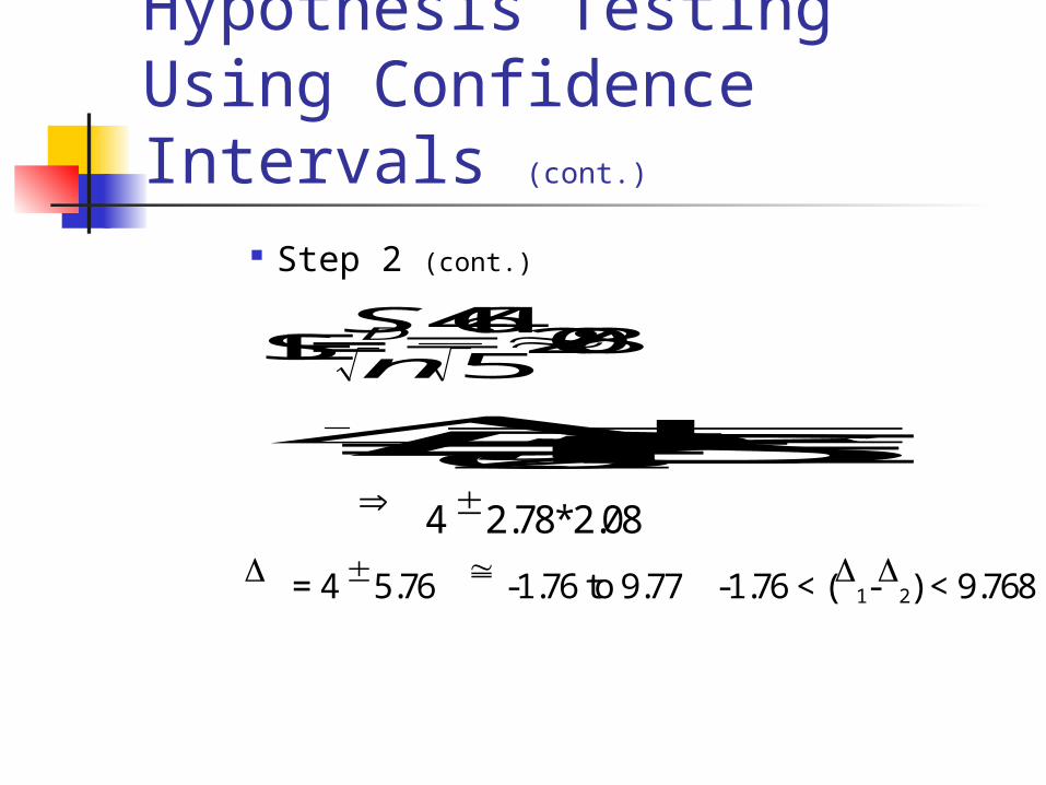
Step 2 (cont.)

SE = SnD464

5208

..

= D t.025 * SE 4 2.78*2.08

= 4 5.76 -1.76 to 9.77 -1.76 < (1-2) < 9.768


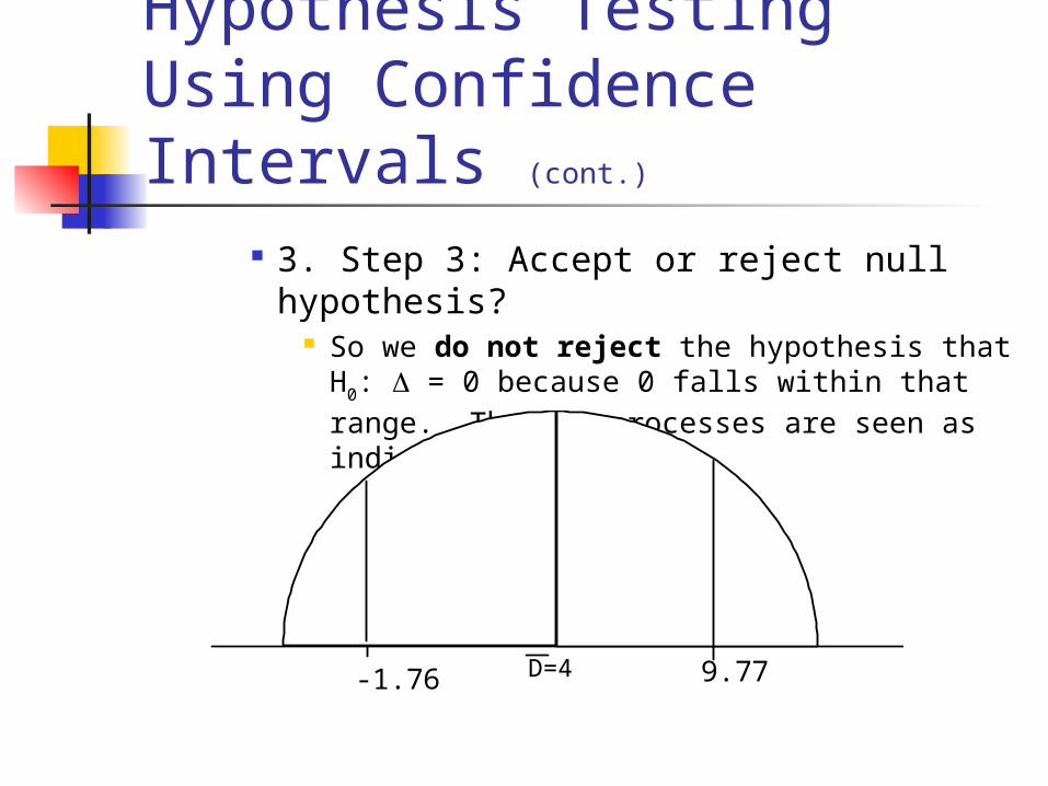
3. Step 3: Accept or reject null hypothesis?

So we do not reject the hypothesis that H0: = 0 because 0 falls within that range. The two processes are seen as indistinguishable.

-1.76 9.77D=4

p-Values III. Method II: p-Values

P-values are essentially the significance level.

In essence, we are calculating the probability that the hypothesis is true. It summarizes the credibility of the null hypothesis.

p-Values A. known

1. Step 1: State the Hypothesis A manufacturing process produces TV. tubes

with an average life=1200 hours and = 300 hours. A new process is thought to give tubes a higher average life. And out of a sample of 100 tubes we find that they have an average life = 1265 hours. Is the new process really any better than the old?

X

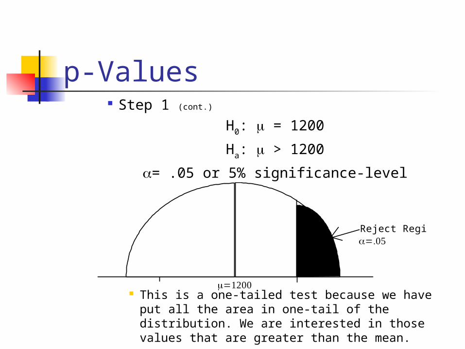
p-Values Step 1 (cont.)

H0: = 1200

Ha: > 1200

= .05 or 5% significance-level

This is a one-tailed test because we have put all the area in one-tail of the distribution. We are interested in those values that are greater than the mean.

Reject Region

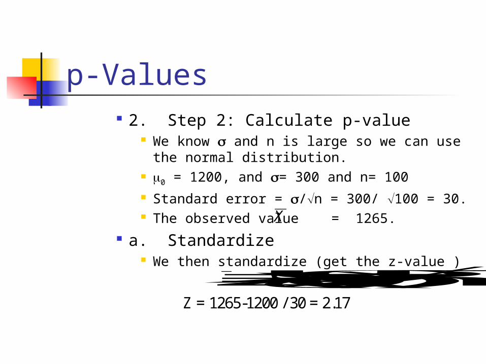
p-Values 2. Step 2: Calculate p-value

We know and n is large so we can use the normal distribution.

0 = 1200, and = 300 and n= 100 Standard error = /n = 300/ 100 = 30. The observed value = 1265.

a. Standardize We then standardize (get the z-value )

X

Z = (X- 0) / (/n) Z = 1265-1200 / 30 = 2.17

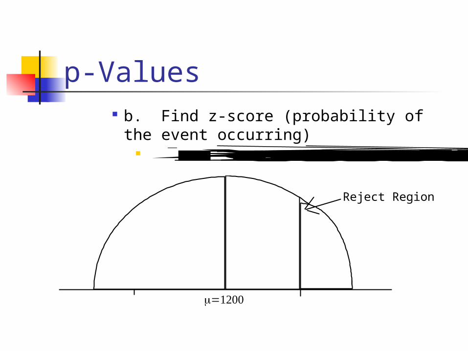
p-Values b. Find z-score (probability of the event

occurring) Pr (X 1265) = Pr(Z 2.17) = .015 (from the z-table)

Reject Region

X=1265

area=1.5%

area=5%

p-Values 3. Step 3: Accept or Reject the

Hypothesis This suggests that if the null hypothesis was

true that there would be only a 1.5% probability of observing as larger as 1265.

Since 1.5% lies to the right of our initial 5% significance level, we can reject the null hypothesis.

X

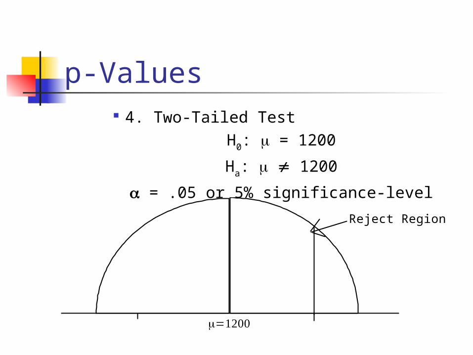
p-Values 4. Two-Tailed Test

H0: = 1200

Ha: 1200

= .05 or 5% significance-level

Reject Region

X=1265

area=1.5%

area=2.5%

Reject Regionarea=2.5%

p-Values Accept or Reject

Since the area to the right of 1265 is only 1.5%, we can again reject H0.

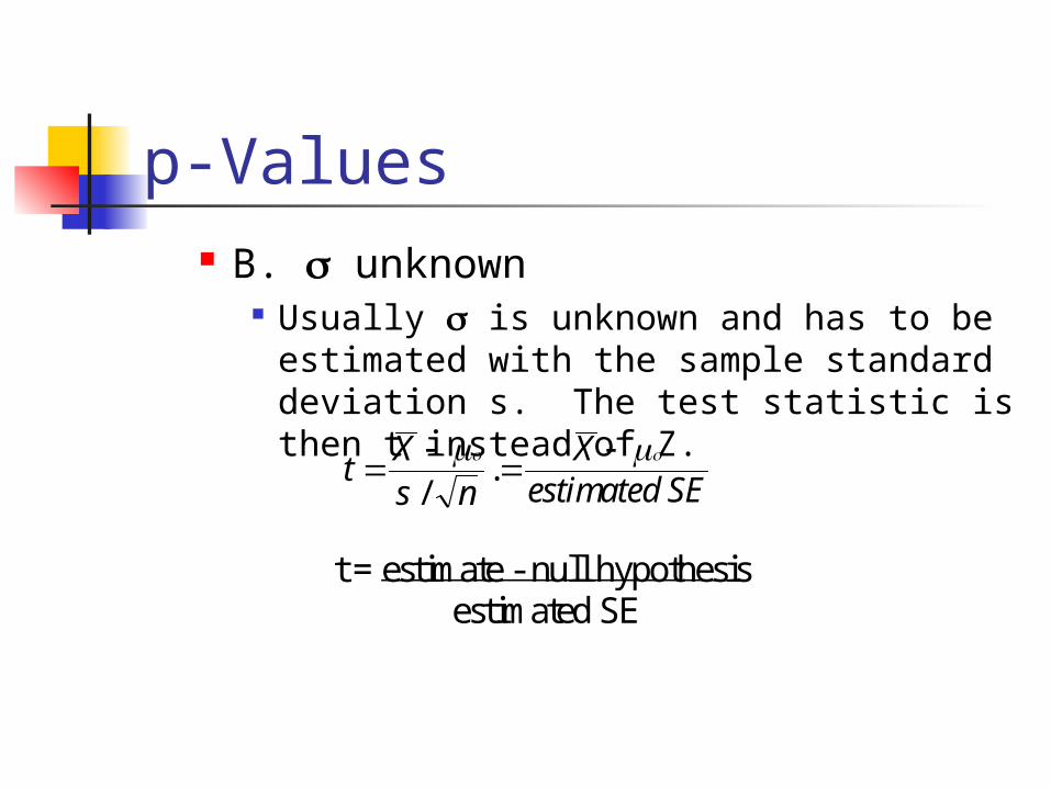
p-Values B. unknown

Usually is unknown and has to be estimated with the sample standard deviation s. The test statistic is then t instead of Z.

tXs n

Xestimated SE

/.

t = estimate - null hypothesis estimated SE

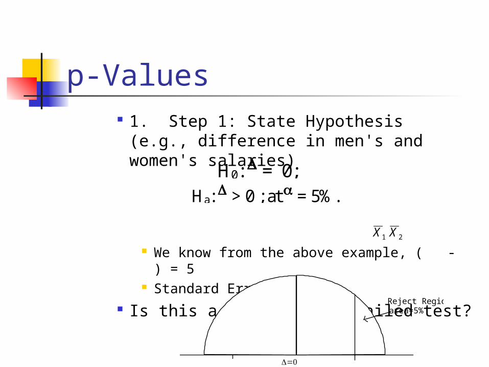
p-Values 1. Step 1: State Hypothesis (e.g.,

difference in men's and women's salaries)

We know from the above example, ( - ) = 5 Standard Error = 1.84

Is this a one or a two tailed test?

H0: = 0; Ha: > 0 ; at = 5%.

X 1 X 2

Reject Regionarea=5%

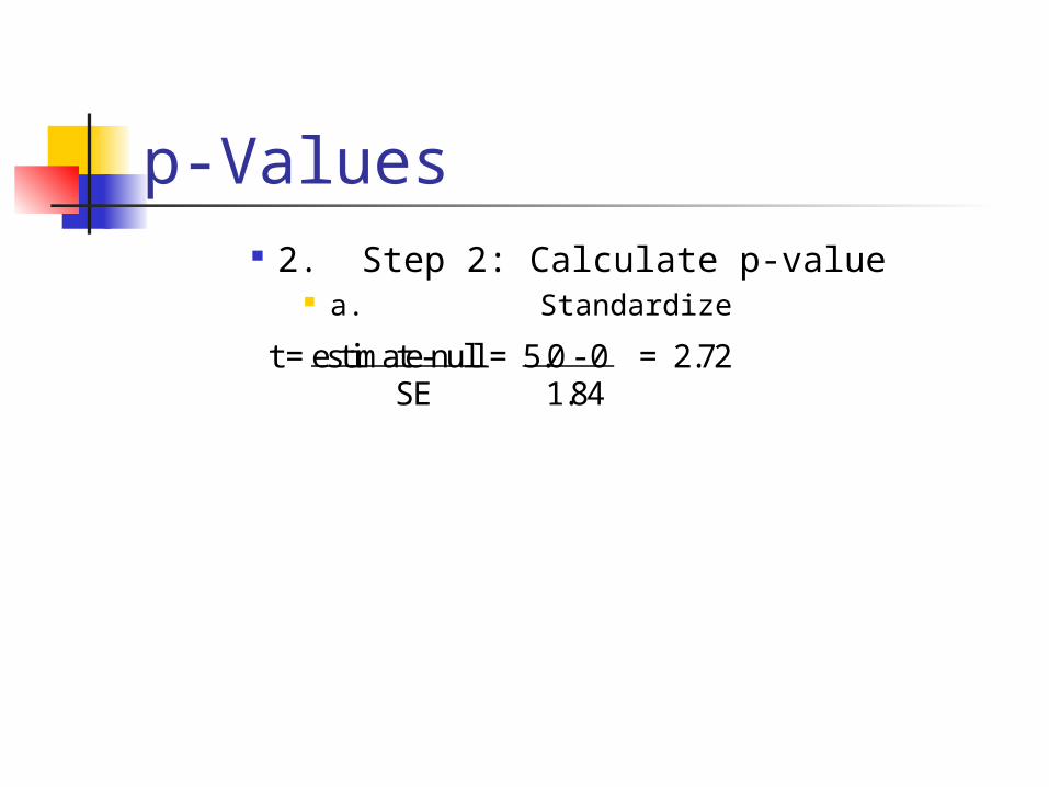
p-Values 2. Step 2: Calculate p-value

a. Standardize

t = estimate-null = 5.0 - 0 = 2.72 SE 1.84

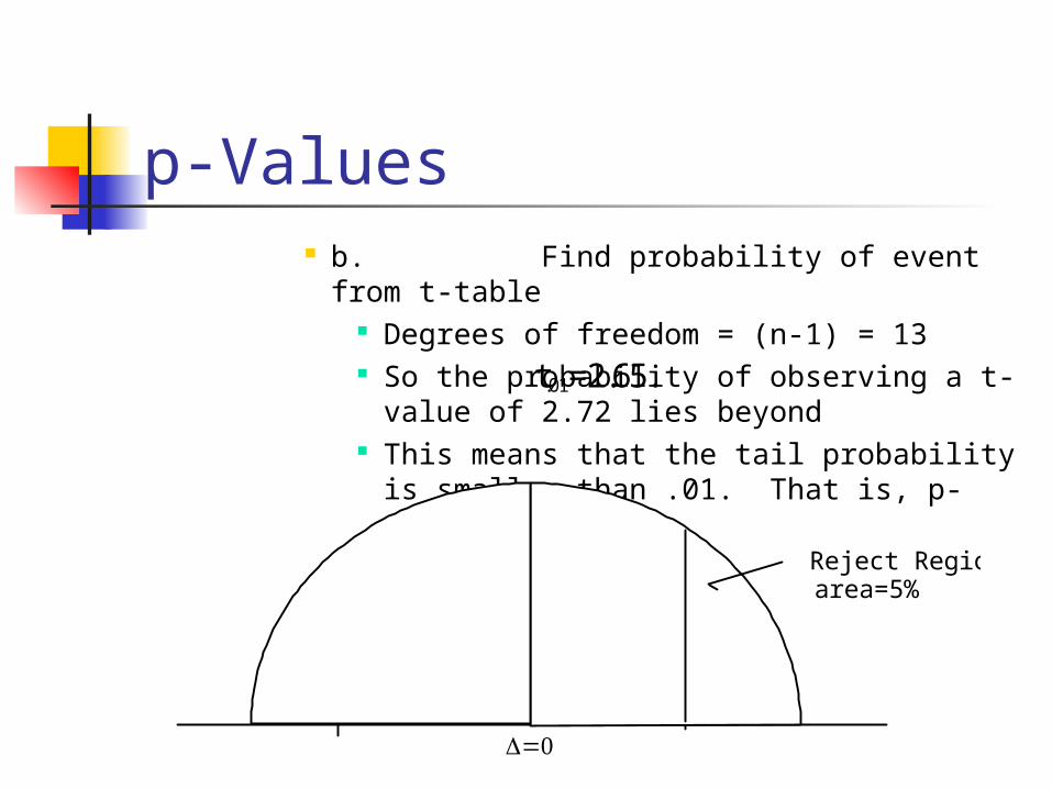
p-Values b. Find probability of event from t-

table Degrees of freedom = (n-1) = 13 So the probability of observing a t-value of

2.72 lies beyond This means that the tail probability is

smaller than .01. That is, p-value < .01.

t.01=2.65.


2.721.77

p-Values 3. Step 3: Accept or Reject Hypothesis

Since the p-value is a measure of the credibility of H0, such a low value (below = 5%) leads us to conclude that H0 is implausible.

Therefore, we reject the null hypothesis.

p-Values C. Getting t-values from Computers

(Review of Homework) 1. Calculate t-values

How does the computer calculate the t-value?

The t-value = (X-)sn

0

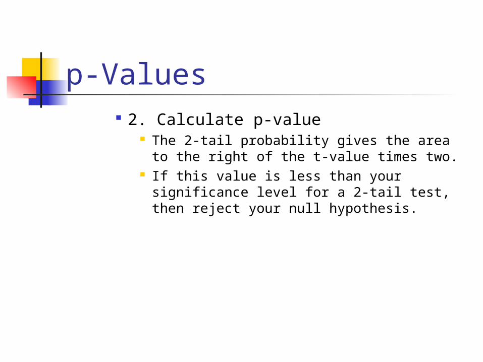
p-Values 2. Calculate p-value

The 2-tail probability gives the area to the right of the t-value times two.

If this value is less than your significance level for a 2-tail test, then reject your null hypothesis.

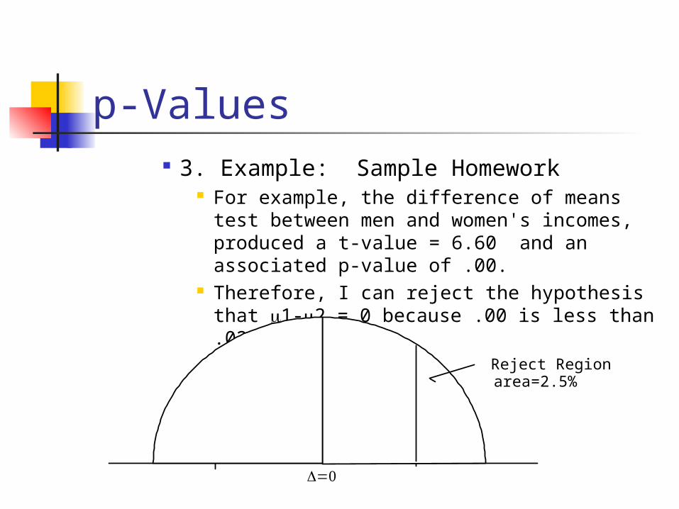
p-Values 3. Example: Sample Homework

For example, the difference of means test between men and women's incomes, produced a t-value = 6.60 and an associated p-value of .00.

Therefore, I can reject the hypothesis that 1-2 = 0 because .00 is less than .025.


6.601.96-1.96

area= .000

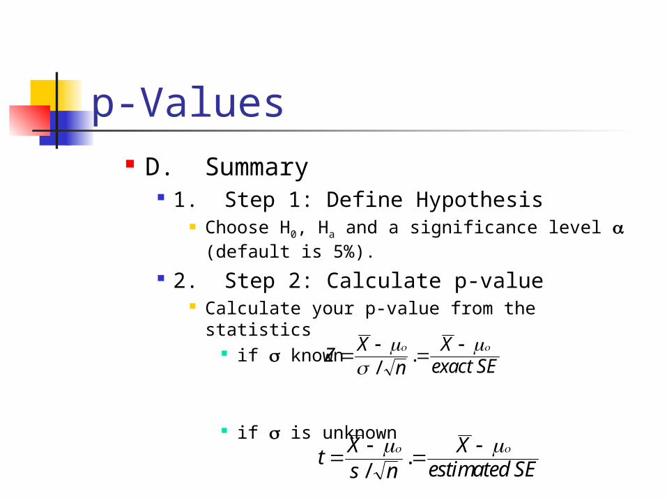
p-Values D. Summary

1. Step 1: Define Hypothesis Choose H0, Ha and a significance level

(default is 5%). 2. Step 2: Calculate p-value

Calculate your p-value from the statistics if known

if is unknown

ZX

nXexact SE

/.

tXs n

Xestimated SE

/.

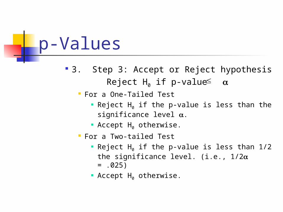
p-Values 3. Step 3: Accept or Reject hypothesis

Reject H0 if p-value For a One-Tailed Test

Reject H0 if the p-value is less than the significance level .

Accept H0 otherwise. For a Two-tailed Test

Reject H0 if the p-value is less than 1/2 the significance level. (i.e., 1/2 = .025)

Accept H0 otherwise.

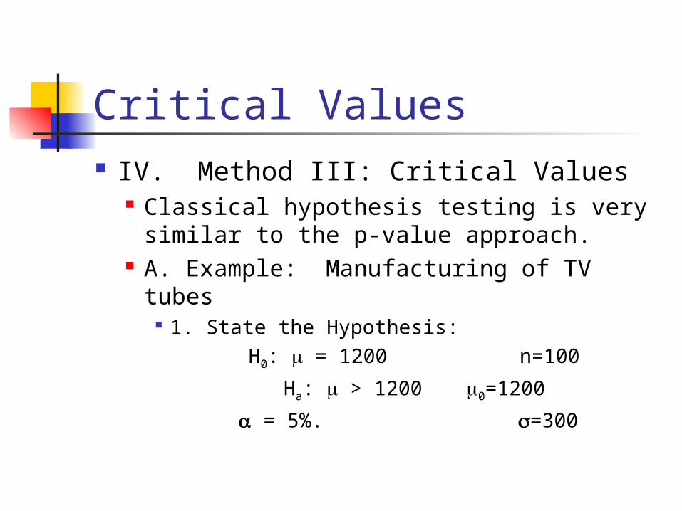
Critical Values IV. Method III: Critical Values

Classical hypothesis testing is very similar to the p-value approach.

A. Example: Manufacturing of TV tubes

1. State the Hypothesis: H0: = 1200 n=100

Ha: > 1200 0=1200

= 5%. =300

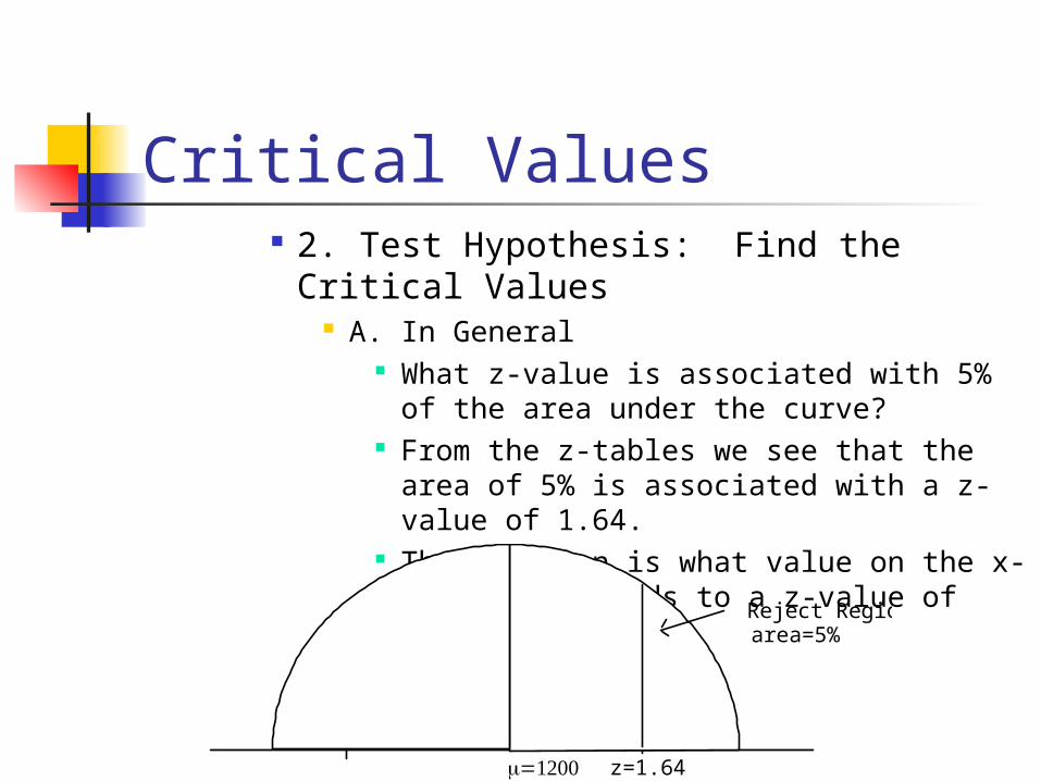
Critical Values 2. Test Hypothesis: Find the Critical

Values A. In General

What z-value is associated with 5% of the area under the curve?

From the z-tables we see that the area of 5% is associated with a z-value of 1.64.

The question is what value on the x-axis corresponds to a z-value of 1.64?


z=1.64

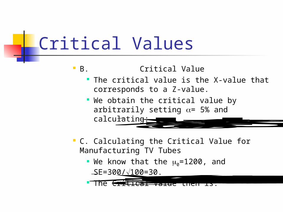
Critical Values B. Critical Value

The critical value is the X-value that corresponds to a Z-value.

We obtain the critical value by arbitrarily setting = 5% and calculating:

C. Calculating the Critical Value for Manufacturing TV Tubes

We know that the 0=1200, and SE=300/100=30.

The Critical Value then is:

Xc = 0 + Z.05*SE

Xc = 1200 + 1.64*30 = 1249.

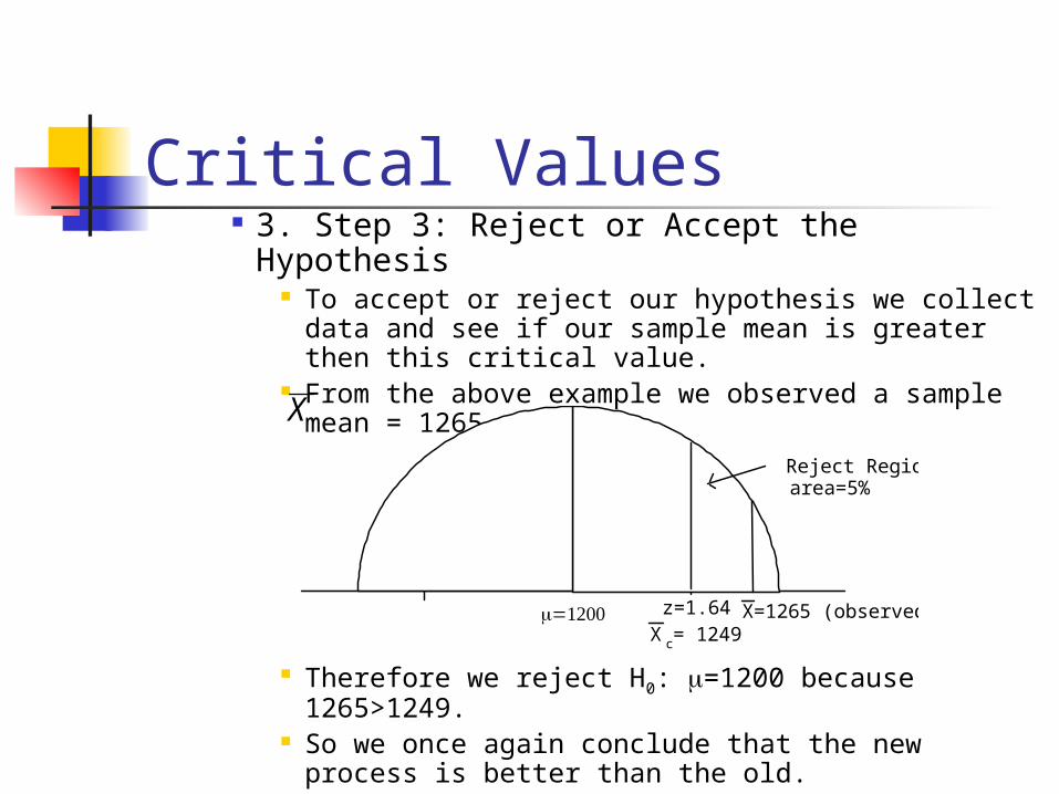
Critical Values 3. Step 3: Reject or Accept the Hypothesis

To accept or reject our hypothesis we collect data and see if our sample mean is greater then this critical value.

From the above example we observed a sample mean = 1265.

Therefore we reject H0: =1200 because 1265>1249.

So we once again conclude that the new process is better than the old.

X


z=1.64X = 1249

c

X=1265 (observed)

Critical Values B. Example of 2-tailed test

How do we construct a two-tailed test at the 5% significance value?

1. Step 1: State Hypothesis H0: = 1200Ha: 1200

= 5%.

Critical Values 2. Step 2: Calculate Critical Value

We use Z.025 instead of Z.05. In this case, we would get c = 0 Z.025*SE.

c = 1200 1.96*30 = 1141 and 1259.

XX

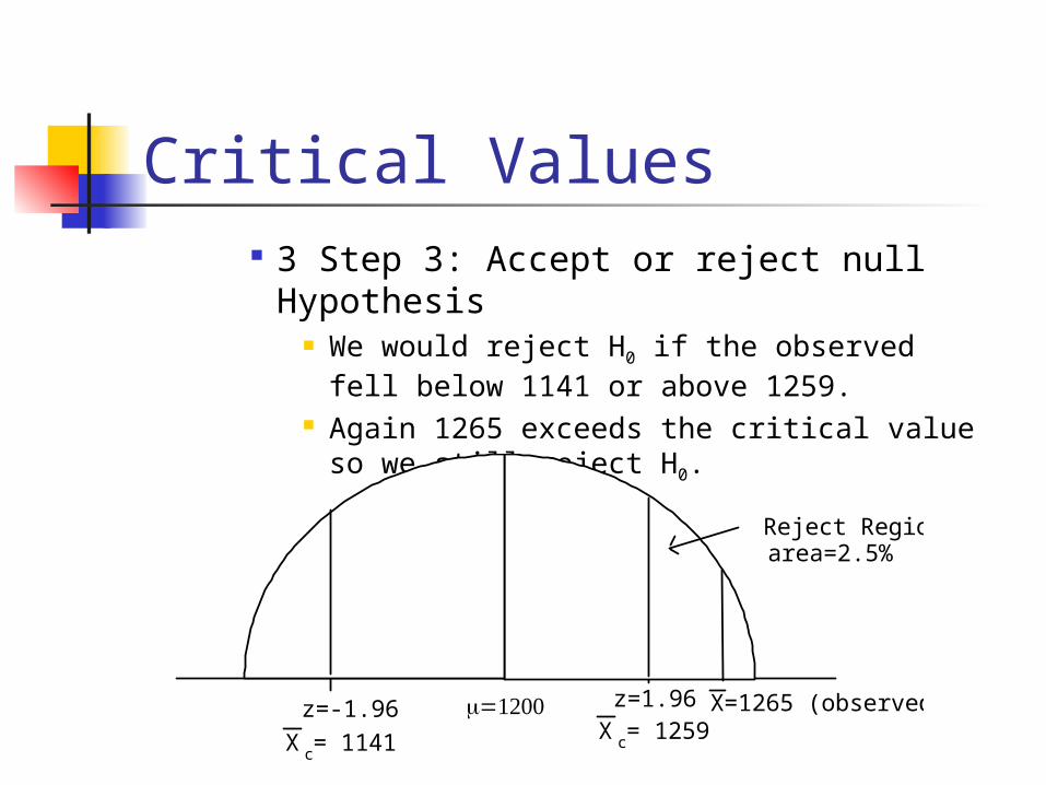
Critical Values 3 Step 3: Accept or reject null Hypothesis

We would reject H0 if the observed fell below 1141 or above 1259.

Again 1265 exceeds the critical value so we still reject H0.


z=1.96X = 1259

c

X=1265 (observed)z=-1.96

X = 1141c

Critical Values C. Summary:

1. Step 1: Define Hypothesis State H0; State Ha; and Choose a significance level .

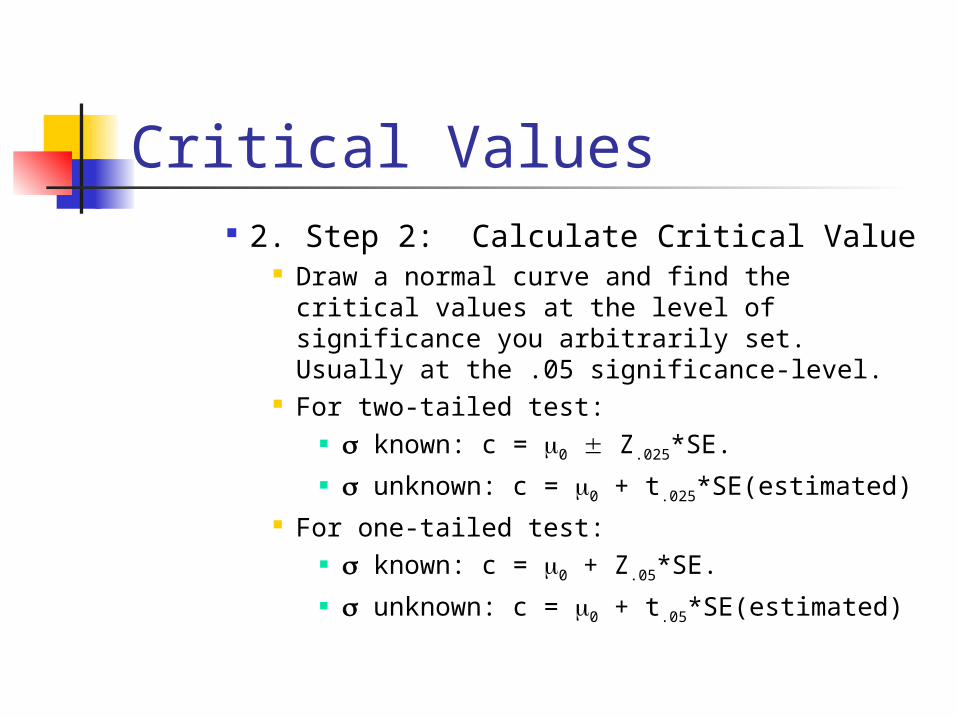
Critical Values 2. Step 2: Calculate Critical Value

Draw a normal curve and find the critical values at the level of significance you arbitrarily set. Usually at the .05 significance-level.

For two-tailed test: known: c = 0 Z.025*SE. unknown: c = 0 + t.025*SE(estimated)

For one-tailed test: known: c = 0 + Z.05*SE. unknown: c = 0 + t.05*SE(estimated)

Critical Values 3. Step 3: Accept or Reject

Then collect sample data. If the sample mean exceeds the critical value,

then reject H0; otherwise accept H0.

Notes About the Exam V. Notes About the Exam

1. Hand in your homework at the beginning of class

2. The exam will cover the material through today's lecture.

3. Problems, no definitions. 4. You may bring a calculator and one 3 X 5

index card with whatever you want written on it.

5. Z-tables and t-tables will be supplied.

Review Session

Review Session: Saturday March 8 11 to 1 PM

Room 411 IAB

statistics and quantitative analysis u4320 segment 7 : hypothesis testing prof. sharyn o’halloran

Documents

hypothesis testingprof

tail tests hypothesis

testing hypotheses

confidence intervals

null hypothesis ho

confidence intervalsii

testing hypothesis1

difference d