lecture 6: variable selection - columbia universityso33/susdev/lecture_6.pdf · lecture 6: variable...
TRANSCRIPT

Lecture 6: Variable Selection
Prof. Sharyn O’Halloran Sustainable Development U9611Econometrics II
Spring 2005 2U9611
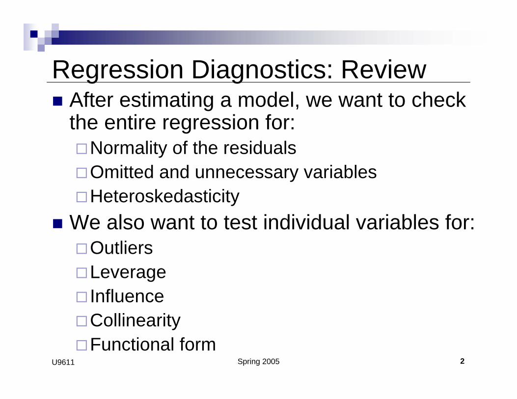
Regression Diagnostics: Review After estimating a model, we want to check the entire regression for:
Normality of the residualsOmitted and unnecessary variablesHeteroskedasticity
We also want to test individual variables for:OutliersLeverageInfluenceCollinearityFunctional form

Spring 2005 3U9611
Look at Residuals: rvfplot
reg price weight mpg forXmpg foreignrvfplot, plotr(lcol(black)) yline(0)
First, examine the residuals ei vs. Y.
Any pattern in the residuals indicates a problem.
Here, there is an obvious U-shape & heteroskedasticity.
^

Spring 2005 4U9611
Check Residuals for NormalityD
ensi
ty
-5000 0 5000 10000
Histogram
Res
idua
ls
Box Plot0
2000
4000
6000
8000
Dis
tanc
e ab
ove
med
ian
0 1000 2000 3000
Symmetry Plo t
Res
idua
ls
-4000 -2000 0 2000 4000
Quantile-Normal Plo t
Residual plots also indicate non-normality
Spring 2005 5U9611
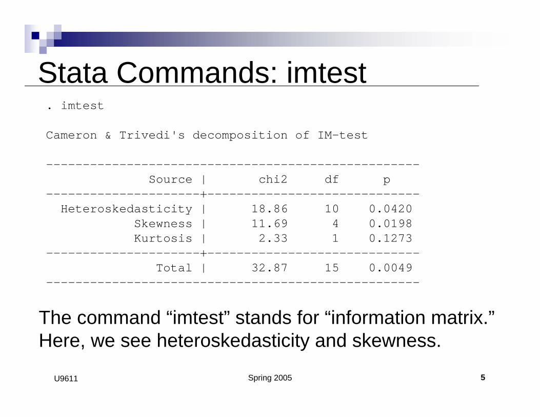
Stata Commands: imtest. imtest
Cameron & Trivedi's decomposition of IM-test
---------------------------------------------------Source | chi2 df p
---------------------+-----------------------------Heteroskedasticity | 18.86 10 0.0420
Skewness | 11.69 4 0.0198Kurtosis | 2.33 1 0.1273
---------------------+-----------------------------Total | 32.87 15 0.0049
---------------------------------------------------
The command “imtest” stands for “information matrix.”Here, we see heteroskedasticity and skewness.
Spring 2005 6U9611
Omitted Variables
Omitted variables are variables that significantly influence Y and so should be in the model, but are excluded.Questions:
Why are omitted variables a problem?How can we test for them?What are the possible fixes?
Let’s check the Venn diagram…
Spring 2005 7U9611
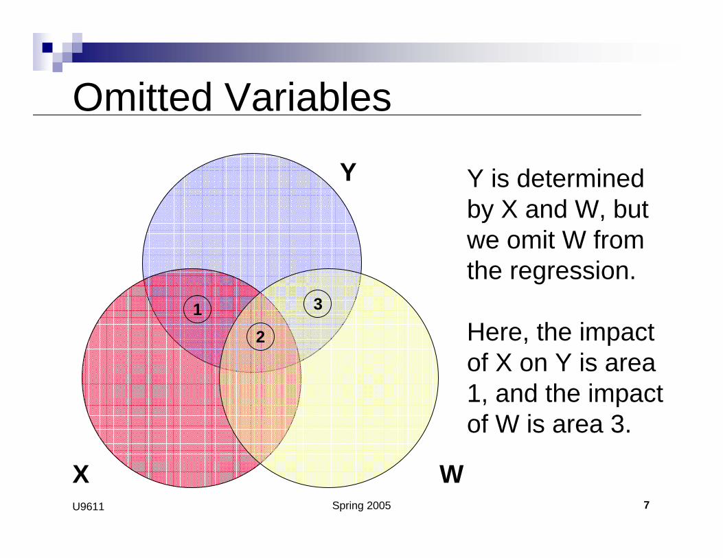
Omitted Variables
Y is determined by X and W, but we omit W from the regression.
Here, the impact of X on Y is area 1, and the impact of W is area 3.
Y
WX
12
3
Spring 2005 8U9611
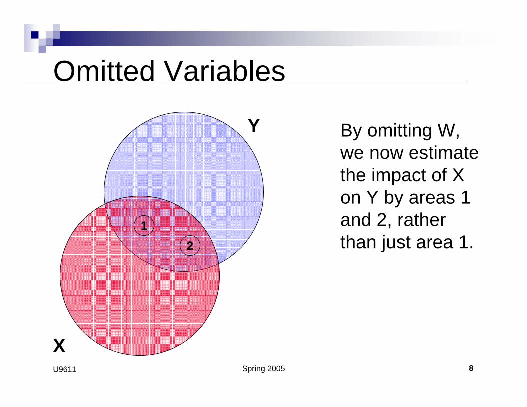
Omitted Variables
By omitting W, we now estimate the impact of X on Y by areas 1 and 2, rather than just area 1.
Y
X
12

Spring 2005 9U9611
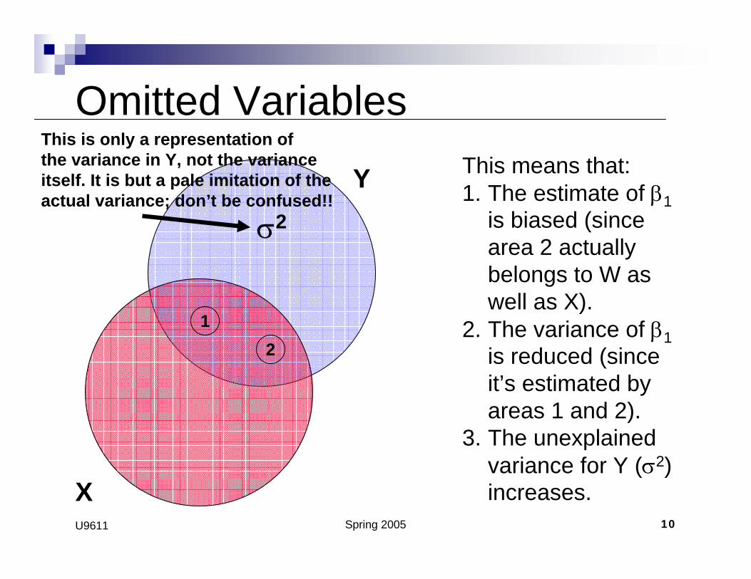
Omitted VariablesThis means that:1. The estimate of β1
is biased (since area 2 actually belongs to W as well as X).
2. The variance of β1is reduced (since it’s estimated by areas 1 and 2).
3. The unexplained variance for Y (σ2) increases.
Y
X
12
σ2
Spring 2005 10U9611
Omitted VariablesThis means that:1. The estimate of β1
is biased (since area 2 actually belongs to W as well as X).
2. The variance of β1is reduced (since it’s estimated by areas 1 and 2).
3. The unexplained variance for Y (σ2) increases.
Y
X
12
σ2
This is only a representation ofthe variance in Y, not the varianceitself. It is but a pale imitation of the actual variance; don’t be confused!!
Spring 2005 11U9611
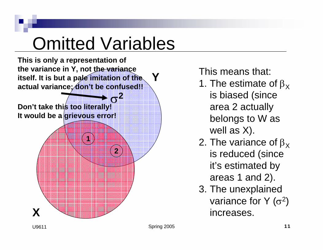
Omitted VariablesThis means that:1. The estimate of βX
is biased (since area 2 actually belongs to W as well as X).
2. The variance of βXis reduced (since it’s estimated by areas 1 and 2).
3. The unexplained variance for Y (σ2) increases.
Y
X
12
σ2
This is only a representation ofthe variance in Y, not the varianceitself. It is but a pale imitation of the actual variance; don’t be confused!!
Don’t take this too literally!It would be a grievous error!

Spring 2005 12U9611
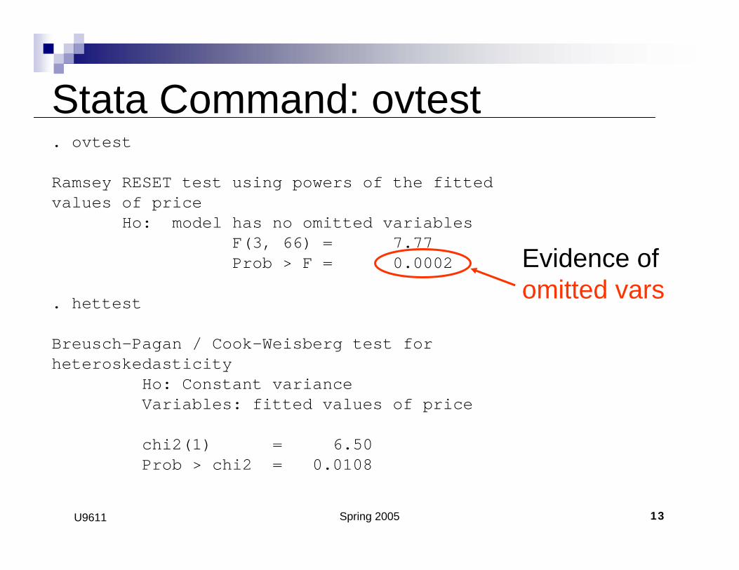
Stata Command: ovtest. ovtest
Ramsey RESET test using powers of the fitted values of price
Ho: model has no omitted variablesF(3, 66) = 7.77Prob > F = 0.0002
. hettest
Breusch-Pagan / Cook-Weisberg test for heteroskedasticity
Ho: Constant varianceVariables: fitted values of price
chi2(1) = 6.50Prob > chi2 = 0.0108
Spring 2005 13U9611
Stata Command: ovtest. ovtest
Ramsey RESET test using powers of the fitted values of price
Ho: model has no omitted variablesF(3, 66) = 7.77Prob > F = 0.0002
. hettest
Breusch-Pagan / Cook-Weisberg test for heteroskedasticity
Ho: Constant varianceVariables: fitted values of price
chi2(1) = 6.50Prob > chi2 = 0.0108
Evidence ofomitted vars
Spring 2005 14U9611
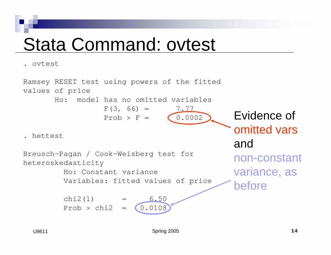
Stata Command: ovtest. ovtest
Ramsey RESET test using powers of the fitted values of price
Ho: model has no omitted variablesF(3, 66) = 7.77Prob > F = 0.0002
. hettest
Breusch-Pagan / Cook-Weisberg test for heteroskedasticity
Ho: Constant varianceVariables: fitted values of price
chi2(1) = 6.50Prob > chi2 = 0.0108
Evidence ofomitted varsandnon-constant variance, as before
Spring 2005 15U9611
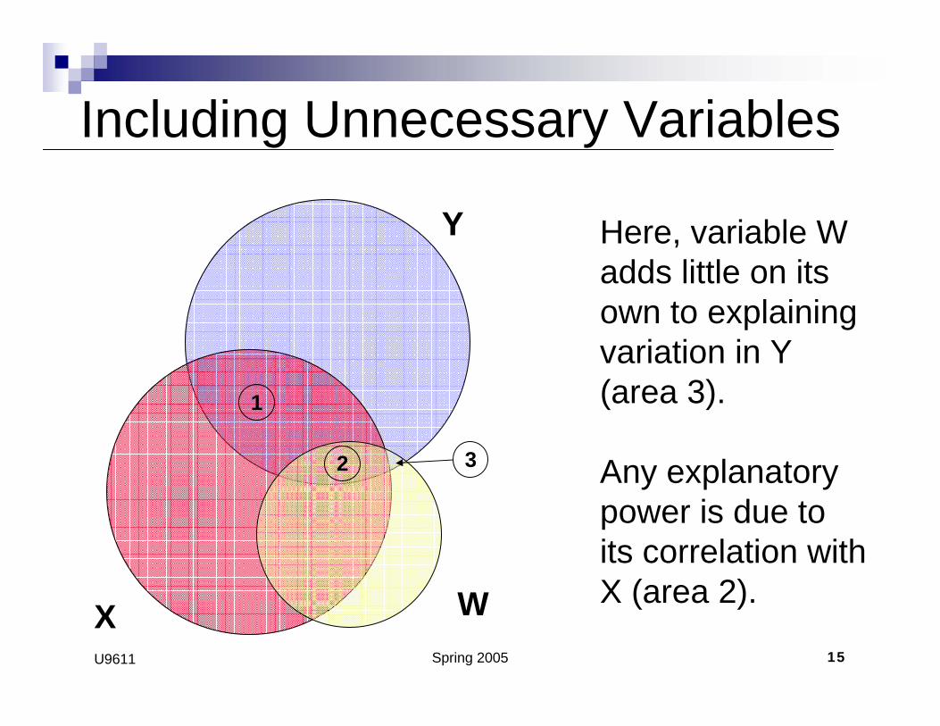
Including Unnecessary Variables
Here, variable W adds little on its own to explaining variation in Y (area 3).
Any explanatory power is due to its correlation with X (area 2).
Y
WX
1
2 3
Spring 2005 16U9611
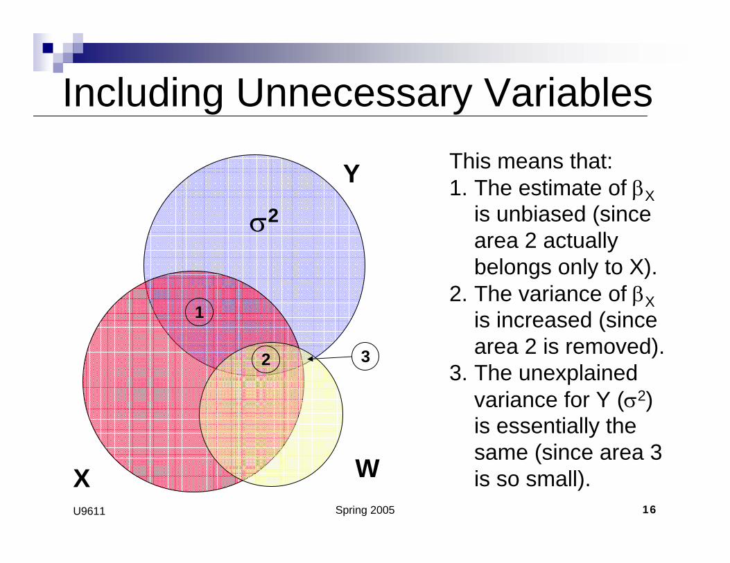
Including Unnecessary Variables
Y
WX
1
2 3
This means that:1. The estimate of βX
is unbiased (since area 2 actually belongs only to X).
2. The variance of βXis increased (since area 2 is removed).
3. The unexplained variance for Y (σ2) is essentially the same (since area 3 is so small).
σ2
Spring 2005 17U9611
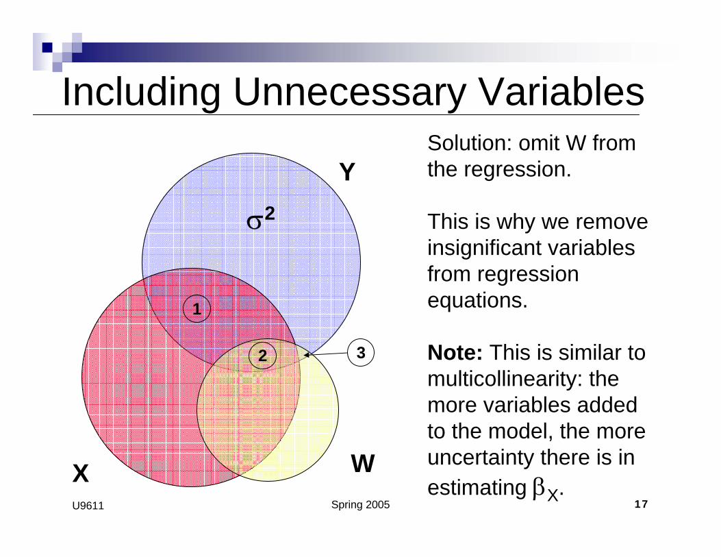
Including Unnecessary Variables
Y
WX
1
2 3
Solution: omit W from the regression.
This is why we remove insignificant variables from regression equations.
Note: This is similar to multicollinearity: the more variables added to the model, the more uncertainty there is in estimating βX.
σ2

Spring 2005 18U9611
Checking Individual VariablesIf the diagnostics on the regression as a whole show potential problems, move to
Checking observations for:LeverageOutliersInfluence
Analyzing the contributions of individual variables to the regression:
AvplotsCprplots
Spring 2005 19U9611
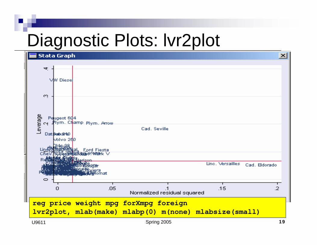
Diagnostic Plots: lvr2plot
reg price weight mpg forXmpg foreignlvr2plot, mlab(make) mlabp(0) m(none) mlabsize(small)
Spring 2005 20U9611
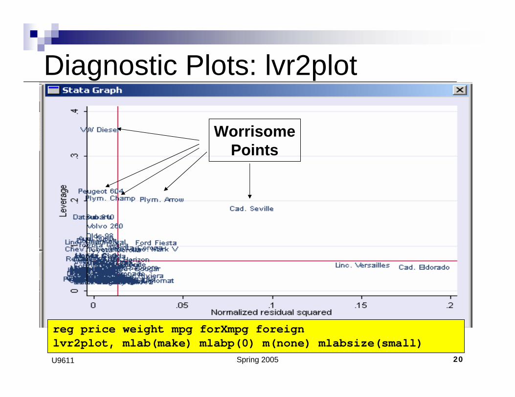
WorrisomePoints
reg price weight mpg forXmpg foreignlvr2plot, mlab(make) mlabp(0) m(none) mlabsize(small)
Diagnostic Plots: lvr2plot

Spring 2005 21U9611
reg price weight mpg forXmpg foreignlvr2plot, mlab(make) mlabp(0) m(none) mlabsize(small)
Diagnostic Plots: lvr2plot
Problem: Only diesel in sampleFix: Could omit

Spring 2005 22U9611
Problem: Data entered incorrectlyFix: Recode!
reg price weight mpg forXmpg foreignlvr2plot, mlab(make) mlabp(0) m(none) mlabsize(small)
Diagnostic Plots: lvr2plot
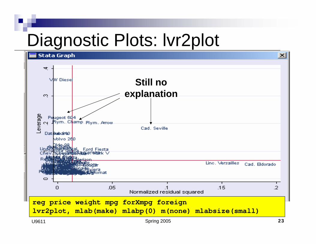
Spring 2005 23U9611
Still noexplanation
reg price weight mpg forXmpg foreignlvr2plot, mlab(make) mlabp(0) m(none) mlabsize(small)
Diagnostic Plots: lvr2plot
Spring 2005 24U9611
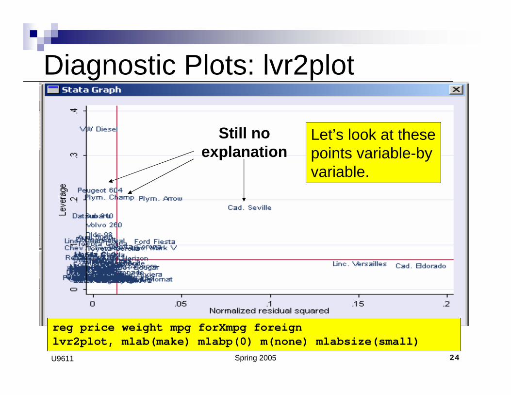
Still noexplanation
reg price weight mpg forXmpg foreignlvr2plot, mlab(make) mlabp(0) m(none) mlabsize(small)
Diagnostic Plots: lvr2plot
Let’s look at thesepoints variable-byvariable.
Spring 2005 25U9611
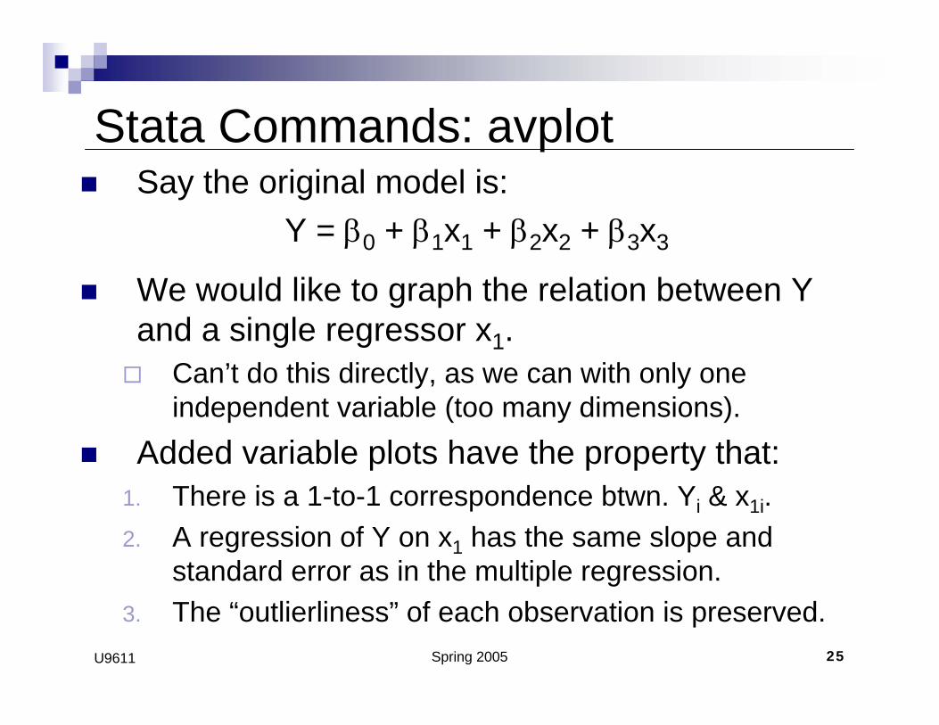
Stata Commands: avplot Say the original model is:
Y = β0 + β1x1 + β2x2 + β3x3
We would like to graph the relation between Y and a single regressor x1.
Can’t do this directly, as we can with only one independent variable (too many dimensions).
Added variable plots have the property that:1. There is a 1-to-1 correspondence btwn. Yi & x1i.2. A regression of Y on x1 has the same slope and
standard error as in the multiple regression.3. The “outlierliness” of each observation is preserved.
Spring 2005 26U9611
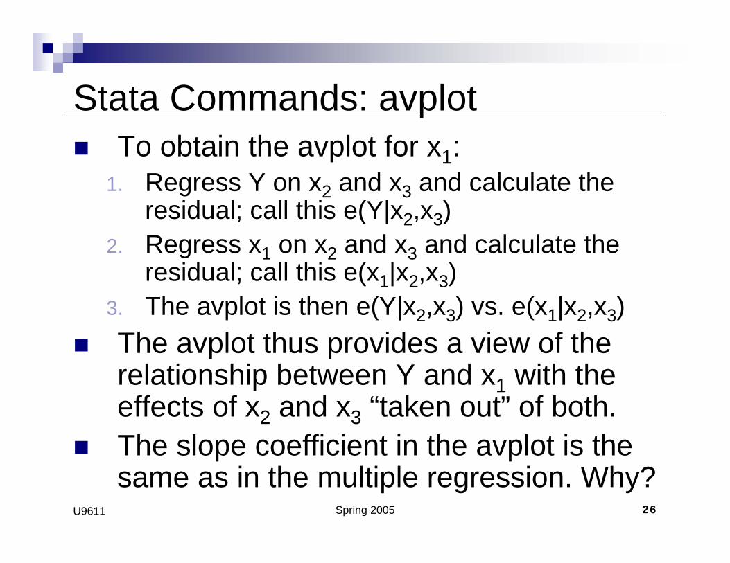
Stata Commands: avplot To obtain the avplot for x1:
1. Regress Y on x2 and x3 and calculate the residual; call this e(Y|x2,x3)
2. Regress x1 on x2 and x3 and calculate the residual; call this e(x1|x2,x3)
3. The avplot is then e(Y|x2,x3) vs. e(x1|x2,x3)The avplot thus provides a view of the relationship between Y and x1 with the effects of x2 and x3 “taken out” of both.The slope coefficient in the avplot is the same as in the multiple regression. Why?

Spring 2005 27U9611
Example: Two Variables
Regress Y on just W first and take the residual.
This takes out areas 2 and 3
Y
WX
12
3
4

Spring 2005 28U9611
Example: Two Variables
Regress Y on just W first and take the residual.
This takes out areas 2 and 3
Note: estimate of βW will be biased.
Y
WX
12
3
4

Spring 2005 29U9611
Example: Two Variables
Y
WX
12
3
4
Now regress X on W and take the residual.

Spring 2005 30U9611
Example: Two Variables
Now regress X on W and take the residual.
This takes out area 4 as well.
Y
WX
12
3
4

Spring 2005 31U9611
Example: Two VariablesIn the resulting figure, the overlap of Y and X is area 1, just as in the original multivariate regression!
That’s why we get the same coefficient
Y
WX
12
3
4

Spring 2005 32U9611
Added variable plots: example- Is the state with largest expenditure influential?- Is there an association of expend and SAT, after accounting for takers?

Spring 2005 33U9611
• Alaska is unusual in its expenditure, and is apparently quite influential

Spring 2005 34U9611
X-axis: residuals after regression expendi = b0 + b1*takersi
Y-axis: residuals after regression SATi = b0 + b1*takersi

Spring 2005 35U9611
After accounting for % of students who take SAT, there is a positive association between expenditure and mean SAT scores.

Spring 2005 36U9611
Component Plus Residual PlotsWe’d like to plot y versus x2 but with the effect of x1subtracted out;
i.e. plot versus x2
To calculate this, get the partial residualpartial residual for x2:
a. Estimate in
b. Use these results to calculate
c. Plot this quantity vs. x2.
Whereas the avplots are better for detecting outliers, cprplots are better for determining functional form.
110 xy ββ −−
210 and ,, βββ εβββ +++= 22110 xxy
ixxy εβββ +=−− 22110

Spring 2005 37U9611
Graph cprplot x1
Graphs each observation's residual plus its component predicted from x1against values of x1i
ii xbe 11+

Spring 2005 38U9611
Graph cprplot x1
Here, the relationship looks fairly linear, although Alaska still has lots of influence.
ii xbe 11+

Spring 2005 39U9611
Regression FixesIf you detect possible problems with your initial regression, you can:
1. Check for mis-coded data2. Divide your sample or eliminate some
observations (like diesel cars)3. Try adding more covariates if the ovtest
turns out positive4. Change the functional form on Y or one of
the regressors5. Use robust regression

Spring 2005 40U9611
Robust RegressionThis is a variant on linear regression that downplays the influence of outliers
1. First performs the original OLS regression2. Drops observations with Cook’s distance > 1 3. Calculates weights for each observation
based on their residuals 4. Performs weighted least squares regression
using these weightsStata command: “rreg” instead of “reg”

Spring 2005 41U9611
Robust Regression: Example. reg mpg weight foreign
Source | SS df MS Number of obs = 74-------------+------------------------------ F( 2, 71) = 69.75
Model | 1619.2877 2 809.643849 Prob > F = 0.0000Residual | 824.171761 71 11.608053 R-squared = 0.6627
-------------+------------------------------ Adj R-squared = 0.6532Total | 2443.45946 73 33.4720474 Root MSE = 3.4071
------------------------------------------------------------------------------mpg | Coef. Std. Err. t P>|t| [95% Conf. Interval]
-------------+----------------------------------------------------------------weight | -.0065879 .0006371 -10.34 0.000 -.0078583 -.0053175foreign | -1.650029 1.075994 -1.53 0.130 -3.7955 .4954422_cons | 41.6797 2.165547 19.25 0.000 37.36172 45.99768
------------------------------------------------------------------------------
This is the original regressionRun the usual diagnostics

Spring 2005 42U9611
Robust Regression: Example-5
05
1015
Res
idua
ls
10 15 20 25 30Fitted values
Residual vs. Fitted Plot

Spring 2005 43U9611
Robust Regression: Example. reg mpg weight foreign
Source | SS df MS Number of obs = 74-------------+------------------------------ F( 2, 71) = 69.75
Model | 1619.2877 2 809.643849 Prob > F = 0.0000Residual | 824.171761 71 11.608053 R-squared = 0.6627
-------------+------------------------------ Adj R-squared = 0.6532Total | 2443.45946 73 33.4720474 Root MSE = 3.4071
------------------------------------------------------------------------------mpg | Coef. Std. Err. t P>|t| [95% Conf. Interval]
-------------+----------------------------------------------------------------weight | -.0065879 .0006371 -10.34 0.000 -.0078583 -.0053175foreign | -1.650029 1.075994 -1.53 0.130 -3.7955 .4954422_cons | 41.6797 2.165547 19.25 0.000 37.36172 45.99768
------------------------------------------------------------------------------
rvfplot shows heterskedasticityAlso, fails a hettest

Spring 2005 44U9611
Robust Regression: Example. rreg mpg weight foreign, genwt(w)
Huber iteration 1: maximum difference in weights = .80280176Huber iteration 2: maximum difference in weights = .2915438Huber iteration 3: maximum difference in weights = .08911171Huber iteration 4: maximum difference in weights = .02697328
Biweight iteration 5: maximum difference in weights = .29186818Biweight iteration 6: maximum difference in weights = .11988101Biweight iteration 7: maximum difference in weights = .03315872Biweight iteration 8: maximum difference in weights = .00721325
Robust regression estimates Number of obs = 74F( 2, 71) = 168.32Prob > F = 0.0000
------------------------------------------------------------------------------mpg | Coef. Std. Err. t P>|t| [95% Conf. Interval]
-------------+----------------------------------------------------------------weight | -.0063976 .0003718 -17.21 0.000 -.007139 -.0056562foreign | -3.182639 .627964 -5.07 0.000 -4.434763 -1.930514_cons | 40.64022 1.263841 32.16 0.000 38.1202 43.16025
------------------------------------------------------------------------------

Spring 2005 45U9611
Robust Regression: Example. rreg mpg weight foreign, genwt(w)
Huber iteration 1: maximum difference in weights = .80280176Huber iteration 2: maximum difference in weights = .2915438Huber iteration 3: maximum difference in weights = .08911171Huber iteration 4: maximum difference in weights = .02697328
Biweight iteration 5: maximum difference in weights = .29186818Biweight iteration 6: maximum difference in weights = .11988101Biweight iteration 7: maximum difference in weights = .03315872Biweight iteration 8: maximum difference in weights = .00721325
Robust regression estimates Number of obs = 74F( 2, 71) = 168.32Prob > F = 0.0000
------------------------------------------------------------------------------mpg | Coef. Std. Err. t P>|t| [95% Conf. Interval]
-------------+----------------------------------------------------------------weight | -.0063976 .0003718 -17.21 0.000 -.007139 -.0056562foreign | -3.182639 .627964 -5.07 0.000 -4.434763 -1.930514_cons | 40.64022 1.263841 32.16 0.000 38.1202 43.16025
------------------------------------------------------------------------------
Note: Coefficient on foreign changes from -1.65 to -3.18

Spring 2005 46U9611
Robust Regression: Example. rreg mpg weight foreign, genwt(w)
Huber iteration 1: maximum difference in weights = .80280176Huber iteration 2: maximum difference in weights = .2915438Huber iteration 3: maximum difference in weights = .08911171Huber iteration 4: maximum difference in weights = .02697328
Biweight iteration 5: maximum difference in weights = .29186818Biweight iteration 6: maximum difference in weights = .11988101Biweight iteration 7: maximum difference in weights = .03315872Biweight iteration 8: maximum difference in weights = .00721325
Robust regression estimates Number of obs = 74F( 2, 71) = 168.32Prob > F = 0.0000
------------------------------------------------------------------------------mpg | Coef. Std. Err. t P>|t| [95% Conf. Interval]
-------------+----------------------------------------------------------------weight | -.0063976 .0003718 -17.21 0.000 -.007139 -.0056562foreign | -3.182639 .627964 -5.07 0.000 -4.434763 -1.930514_cons | 40.64022 1.263841 32.16 0.000 38.1202 43.16025
------------------------------------------------------------------------------
This command saves the weights generated by rreg

Spring 2005 47U9611
Robust Regression: Example
This shows that three observations were dropped by the rreg, including the VW Diesel
. sort w
. list make mpg weight w if w<.467, sep(0)
+-------------------------------------------+| make mpg weight w ||-------------------------------------------|
1. | Subaru 35 2,050 0 |2. | VW Diesel 41 2,040 0 |3. | Datsun 210 35 2,020 0 |4. | Plym. Arrow 28 3,260 .04429567 |5. | Cad. Seville 21 4,290 .08241943 |6. | Toyota Corolla 31 2,200 .10443129 |7. | Olds 98 21 4,060 .28141296 |
+-------------------------------------------+

Spring 2005 48U9611
Theories, Tests and ModelsQuestion: Which variables should we include on the RHS of our estimation?This is a fundamental question of research design and testing.
NOT merely a mechanical process.So let’s first review some basic concepts of theory-driven research.
Theory-driven = based on a model of the phenomenon of interest, formal or otherwise.We always do this, somehow, in our research

Spring 2005 49U9611
Theories, Tests and Models
Say we have a theory predicting IV1, IV2, and IV3 all affect dependent variable Y.
Dep. Var.
IV1
IV2
IV3

Spring 2005 50U9611
Theories, Tests and Models
Say we have a theory predicting IV1, IV2, and IV3 all affect dependent variable Y.
Dep. Var.
IV1
IV2
IV3
Model

Spring 2005 51U9611
Theories, Tests and Models
Say we have a theory predicting IV1, IV2, and IV3 all affect dependent variable Y.
Dep. Var.
IV1
IV2
IV3
Model
Data-GeneratingProcess (DGP)

Spring 2005 52U9611
Theories, Tests and Models
For instance:
Dep. Var.
IV1
IV2
IV3

Spring 2005 53U9611
Theories, Tests and Models
For instance:1. Congressional Committee ideal points,
Dep. Var.
C
IV2
IV3

Spring 2005 54U9611
Theories, Tests and Models
For instance:1. Congressional Committee ideal points, 2. The President’s ideal point, and
Dep. Var.
C
P
IV3

Spring 2005 55U9611
Theories, Tests and Models
For instance:1. Congressional Committee ideal points, 2. The President’s ideal point, and 3. Uncertainty in the policy area
Dep. Var.
C
P
U

Spring 2005 56U9611
Theories, Tests and Models
For instance:1. Congressional Committee ideal points, 2. The President’s ideal point, and 3. Uncertainty in the policy area
Affect Delegation to the executive.
Delegation
C
P
U

Spring 2005 57U9611
Theories, Tests and Models
Question: What if another variable is suggested that might also impact Y?
Delegation
C
P
U

Spring 2005 58U9611
Theories, Tests and Models
Question: What if another variable is suggested that might also impact Y?For instance, the Interest group environment surrounding the issue.
Delegation
C
P
UI?

Spring 2005 59U9611
Theories, Tests and ModelsRemember: our original regression variables came from a particular model of our subject.There are, generally, three options when new variables are suggested:
1. Re-solve the model with the new variable(s)included as well;
2. Assume the model is a complete Data Generating Process (DGP) and ignore other potential factors;
3. Treat the model as a partial DGP.
We will consider each in turn.

Spring 2005 60U9611
Add New Variables to the ModelWe could expand our model to include the new variable(s).
Formal models: re-solve the equilibriumQualitative models: re-evaluate the predicted effects
In the long run, though, this is not feasibleThere will always be more factors that might affect the phenomenon of interestDon’t want to take the position that you can’t have a theory of anything without having a theory of everything

Spring 2005 61U9611
Treat the Model as a Complete DGPThis means to just look at the impact of the variables suggested by your theory on the dependent variableThis is unrealistic, but an important first cut at the problemYou can do this with
Naturally occuring dataExperimental data
Either way, this is a direct test of the theory

Spring 2005 62U9611
Treat the Model as a Partial DGPThis is the modal response – just add the new variables to the estimation modelBut it has some shortcomings:
You lose the advantages of modellingYou’re not directly testing your theory any more, but rather your theory plus some conjectures.Have to be careful about how the error term enters the equation – where does ε come from?
If you do this, best to use variables already known to affect the dependent variable.

Spring 2005 63U9611
How To Handle Many RegressorsWith this in mind, how can we handle a situation where we have many potential indep. variables?
Two good reasons for seeking a subset of these:General principle: smaller is better (Occam’s razor)
Unnecessary terms add imprecision to inferences
Computer assisted toolsFit of all possible models (include or exclude each X) Compare with these statistics:
Cp, AIC, or BIC
Stepwise regression (search along favorable directions)
But don’t expect a BEST or a TRUE model or a law of nature

Spring 2005 64U9611
Objectives when there are many X’s (12.2.1)
AssessmentAssessment of one X, after accounting for many others
Ex: Do males receive higher salaries than females, after accounting for legitimate determinants of salary?Strategy: first find a good set of X’s to explain salary; then see if the sex indicator is significant when added
Fishing for associationFishing for association; i.e. what are the important X’s?
The trouble with this: we can find several subsets of X’s that explain Y; but that doesn’t imply importance or causationBest attitude: use this for hypothesis generation
PredictionPredictionThis is a straightforward objectiveFind a useful set of X’s; no interpretation required

Spring 2005 65U9611
Loss of precision due to multicollinearity
Review: variance of L.S. estimator of slope in simple reg. =
Fact: variance of L.S. estimator of coef. of Xj in mult. reg. =
)1()1(
)1(
22
2
2
2
jj
x
Rsn
sn
−−
−
σ
σ
R2 in the regressionof Xj on the
other X’s in modelSample variance
of Xj
Sample varianceof X
Variance about
the regression

Spring 2005 66U9611
Implications of MulticollinearitySo variance of an estimated coef. will tend to be larger if there are other X’s in the model that can predict Xj.The S.E. of prediction will also tend to be larger if there are unnecessary or redundant X’s in the model.The tradeoff for adding more regressors is:
You explain more of the variance in Y, butYou estimate the impact of all other variables on Y using less information

Spring 2005 67U9611
Multicollinearity: The situation in which is small for oneor more j’s (usually characterized by highly correlated X’s).
Strategy: There isn’t a real need to decide whether multicollinearity is or isn’t present, as long as one tries to find a subset of x’s that adequately
explains µ(Y), without redundancies.
“Good” subsets of x’s: (a) lead to a small (b) with as few x’s as possible (Criteria Cp, AIC, and BIC formalize this)
2σ̂
)1( 22jj Rs −
Implications of Multicollinearity

Spring 2005 68U9611
Strategy for dealing with many X’s1. Identify objectives; identify relevant set of
X’s2. Exploration:
matrix of scatterplots; correlation matrix; Residual plots after fitting tentative models
3. Resolve transformation and influence before variable selection
4. Computer-assisted variable selection:Best:
Compare all possible subset models using either Cp, AIC, or BIC; find some model with a fairly small value
Next best: Use sequential variable selection, like stepwise regression (this doesn’t look at all possible subset models, but may be more convenient with some statistical programs)

Spring 2005 69U9611
Sequential Variable Selection1. Forward selection
a. Start with no X’s “in” the model St 412/512 page 98.b. Find the “most significant” additional X (with an F-test).c. If its p-value is less than some cutoff (like .05) add it to the model (and re-fit the model with the new set of X’s).d. Repeat (b) and (c) until no further X’s can be added.
2. Backward eliminationa. Start with all X’s “in” the mode.lb. Find the “least significant” of the X’s currently in the model.c. If it’s p-value is greater than some cutoff (like .05) drop itfrom the model (and re-fit with the remaining x’s).d. Repeat until no further X’s can be dropped.

Spring 2005 70U9611
3. Stepwise regressiona) Start with no X’s “in” St 412/512 page 99
b) Do one step of forward selection
c) Do one step of backward elimination
d) Repeat (b) and (c) until no further X’s can be added or dropped
4. NotesNotesa) Add and drop factor indicator variables as a group
b) Don’t take p-values and CI’s for selected variables seriously—because of serious data snooping (not a problem for objectives 1 and 3)
c) A drawback: the product is a single model. This is deceptive.
Think not: “here is the best model.”
Think instead: “here is one, possibly useful model.”
Sequential Variable Selection (cont.)

Spring 2005 71U9611
Criteria for Comparing Models

Spring 2005 72U9611
1. The proposed criteria: Mallow’s Cp Statistic, Schwarz’s Bayesian Information Criterion (BIC or SBC), and Akaike’sInformation Criterion (AIC)
2. The idea behind these is the same, but the theory for arriving at the trade-off between small and small p differs
3. My opinion: there’s no way to truly say that one of these Criteria is better than the others
4. Computer programs: Fit all possible models; report the best 10 or so according to the selected criteria
5. Note: one other criteria: + 0 (sometimes used; but isn’t As good). An equivalent criterion is - (see Sect.10.4.1)
2σ̂
2AdjustedR
2σ̂
Comparing Models (continued)

Spring 2005 73U9611
Cross Validation (12.6.4)
If tests, CIs, or prediction intervals are needed after Variable selection and if n is large, maybe try:Cross validation
Randomly divide the data into 75% for model construction and 25% for inferencePerform variable selection with the 75%Refit the same model (don’t drop or add anything) on the remaining 25% and proceed with inference using that fit.

Spring 2005 74U9611
Example: Sex Discrimination

Spring 2005 75U9611
Example: Sex Discrimination

Spring 2005 76U9611
Example: Sex Discrimination

Spring 2005 77U9611
Example: Sex Discrimination

Spring 2005 78U9611
Example: Sex Discrimination

Spring 2005 79U9611
Example: Sex DiscriminationAll possible regressions in Stata
using commands window