lecture 1: data and models - columbia universityso33/susdev/lecture_1.pdf · lecture 1: data and...
TRANSCRIPT

Lecture 1: Data and Models
Prof. Sharyn O’Halloran Sustainable Development U9611Econometrics II
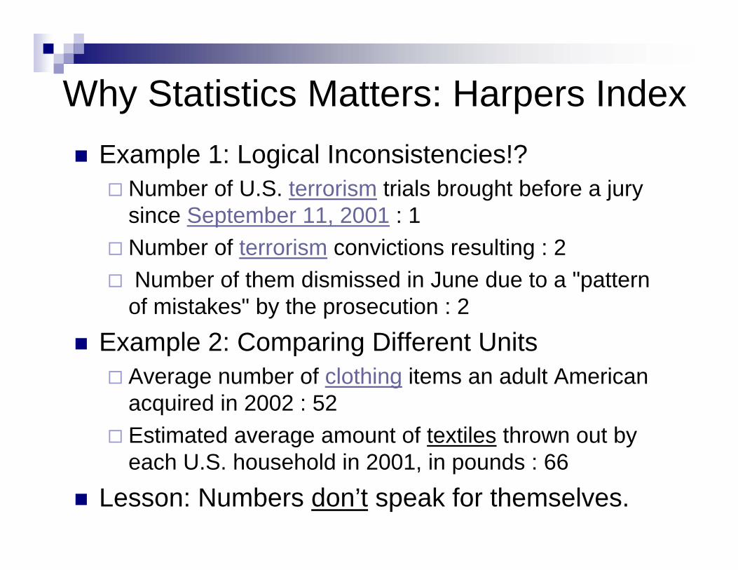
Why Statistics Matters: Harpers IndexExample 1: Logical Inconsistencies!?
Number of U.S. terrorism trials brought before a jury since September 11, 2001 : 1 Number of terrorism convictions resulting : 2Number of them dismissed in June due to a "pattern of mistakes" by the prosecution : 2
Example 2: Comparing Different UnitsAverage number of clothing items an adult American acquired in 2002 : 52 Estimated average amount of textiles thrown out by each U.S. household in 2001, in pounds : 66
Lesson: Numbers don’t speak for themselves.
General Approach: Data VisualizationStandard econometric approach emphasizes:
Calculating the variance-covariance matrixApplying “fixes” to get the right answer
Ease of statistical programs and increased computing power emphasis has shifted to a multifaceted view of data analysis
Graphical presentationQuestion driven estimationInterpretation and inference
General Approach: Question DrivenModeling complex social science phenomena become a series of choices:
What is the process by which the data will be generated?
RandomExperimental Observational
What is the appropriate estimation techniques?LinearProbabilistic
What is the scope of inference?How general are the findings?Has a lot to do with the research design.
Game PlanExamine variables individually
Transform variables as neededExamine key relationsIdentify appropriate estimation techniques
OLS, Probit, Logit, etc…Define model specification
Which variables to include in the analysisDerived both from inspection of the data and theory
Then run analysis Perform post-regression diagnostics
Tests for significance, graphical analysis, simulationsRepeat!
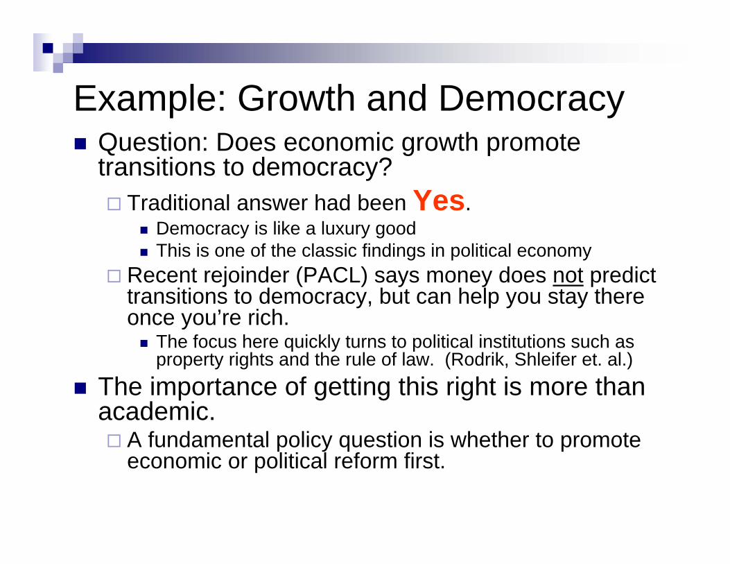
Example: Growth and DemocracyQuestion: Does economic growth promote transitions to democracy?
Traditional answer had been Yes.Democracy is like a luxury goodThis is one of the classic findings in political economy
Recent rejoinder (PACL) says money does not predict transitions to democracy, but can help you stay there once you’re rich.
The focus here quickly turns to political institutions such as property rights and the rule of law. (Rodrik, Shleifer et. al.)
The importance of getting this right is more than academic.
A fundamental policy question is whether to promote economic or political reform first.
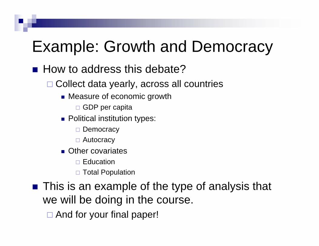
Example: Growth and DemocracyHow to address this debate?
Collect data yearly, across all countriesMeasure of economic growth
GDP per capitaPolitical institution types:
DemocracyAutocracy
Other covariatesEducation Total Population
This is an example of the type of analysis that we will be doing in the course.
And for your final paper!
Example: Growth and Democracy
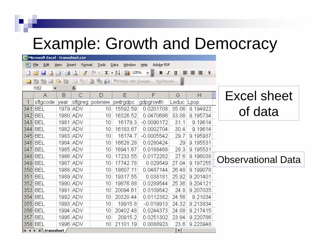
Excel sheet of data
Observational Data
Example: Growth and Democracy
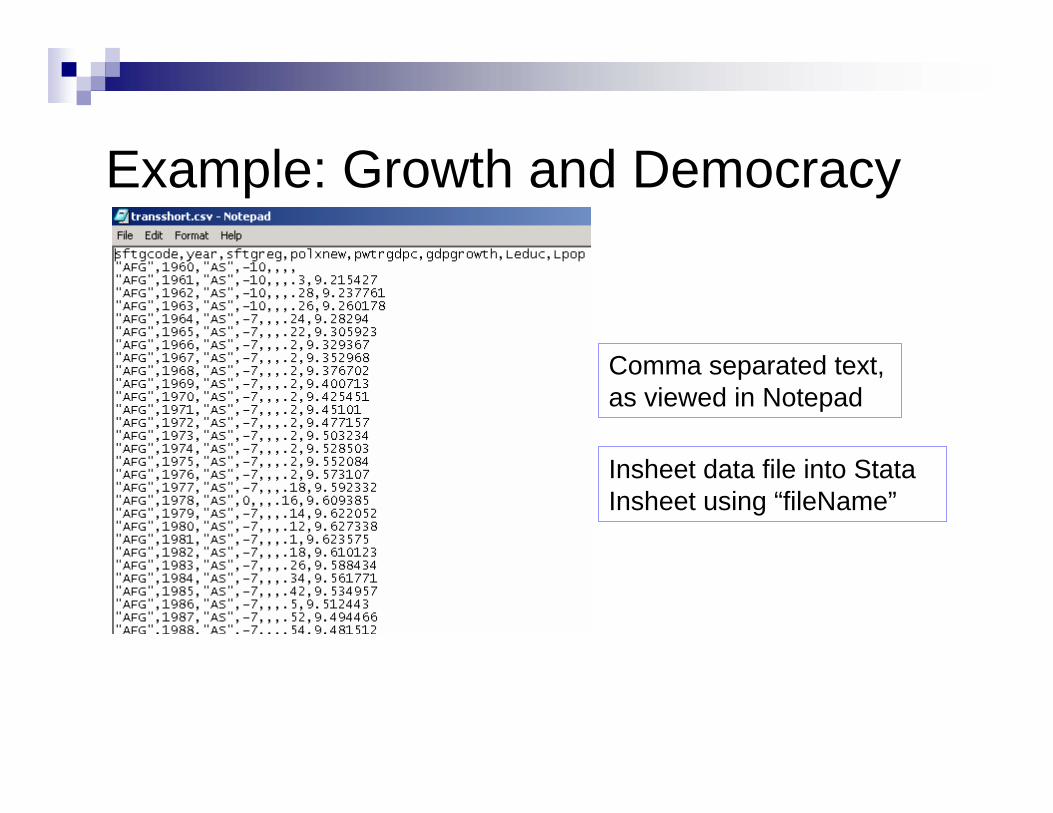
Comma separated text, as viewed in Notepad
Insheet data file into StataInsheet using “fileName”
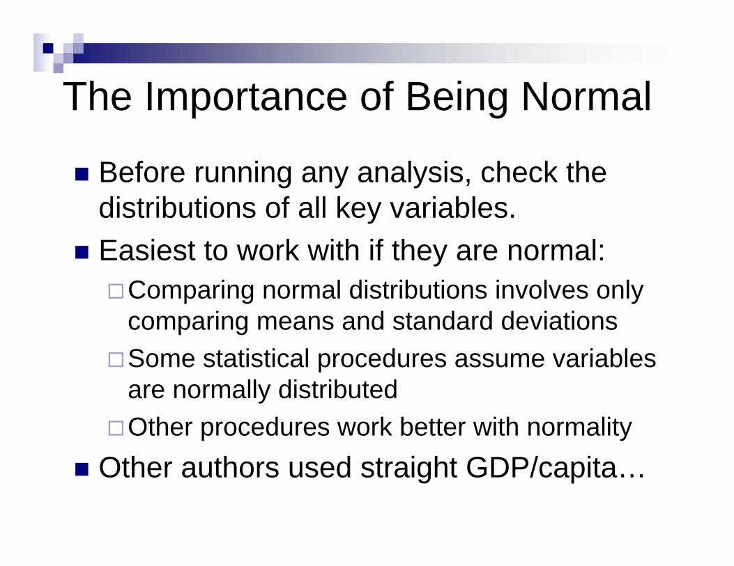
The Importance of Being Normal
Before running any analysis, check the distributions of all key variables.Easiest to work with if they are normal:
Comparing normal distributions involves only comparing means and standard deviationsSome statistical procedures assume variables are normally distributedOther procedures work better with normality
Other authors used straight GDP/capita…
Example: Growth and Democracy
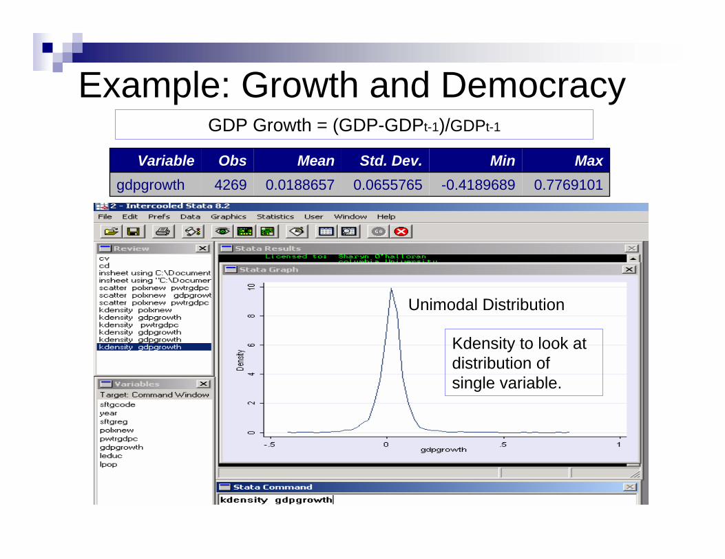
Kdensity to look at distribution of single variable.
GDP Growth = (GDP-GDPt-1)/GDPt-1
Unimodal Distribution
0.7769101-0.41896890.06557650.01886574269gdpgrowthMaxMinStd. Dev.MeanObsVariable
Example: Growth and Democracy
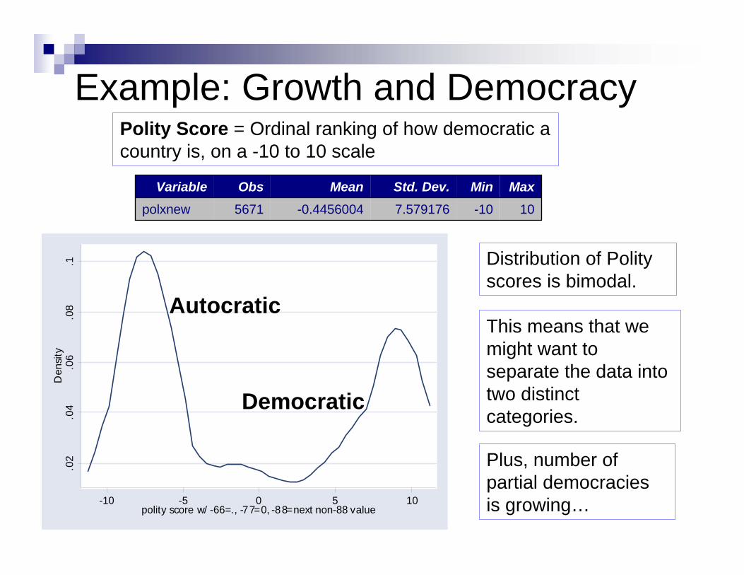
Distribution of Polity scores is bimodal.
Polity Score = Ordinal ranking of how democratic a country is, on a -10 to 10 scale
10-107.579176-0.44560045671polxnew
MaxMinStd. Dev.MeanObsVariable
.02
.04
.06
.08
.1D
ensi
ty
-10 -5 0 5 10polity score w/ -66=., -77=0, -88=next non-88 value
Democratic
AutocraticThis means that we might want to separate the data into two distinct categories.
Plus, number of partial democracies is growing…
Example: Growth and Democracy0
.2.4
.6.8
1
1960
1961
1962
1963
1964
1965
1966
1967
1968
1969
1970
1971
1972
1973
1974
1975
1976
1977
1978
1979
1980
1981
1982
1983
1984
1985
1986
1987
1988
1989
1990
1991
1992
1993
1994
1995
1996
1997
1998
1999
2000
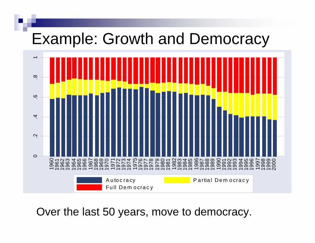
A u to c ra cy P a rtia l De m o cra c yFu ll De m o cra c y
Over the last 50 years, move to democracy.
The Importance of Being Normal
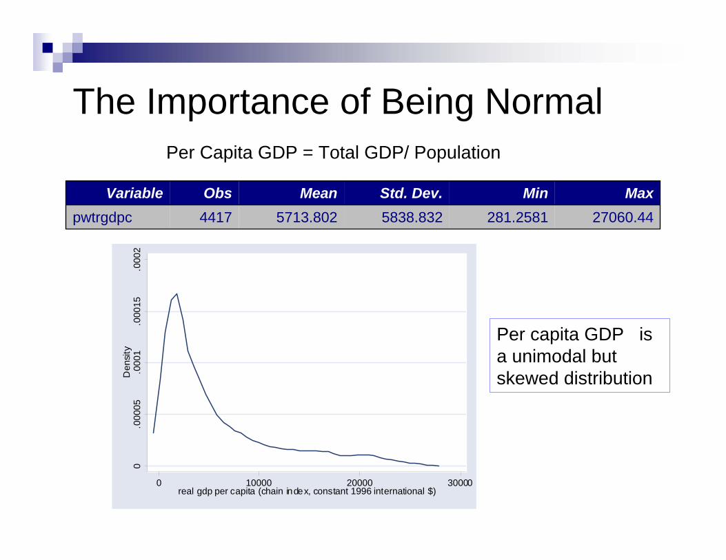
Per capita GDP is a unimodal but skewed distribution
Per Capita GDP = Total GDP/ Population
27060.44281.25815838.8325713.8024417pwtrgdpcMaxMinStd. Dev.MeanObsVariable
0.0
0005
.000
1.0
0015
.000
2D
ensi
ty
0 10000 20000 30000real gdp per capita (chain index, constant 1996 international $)
The Importance of Being Normal0
10,0
0020
,000
30,0
00re
al gd
p pe
r ca
pita
(cha
in in
dex,
con
stan
t 199
6 in
tern
atio
nal $
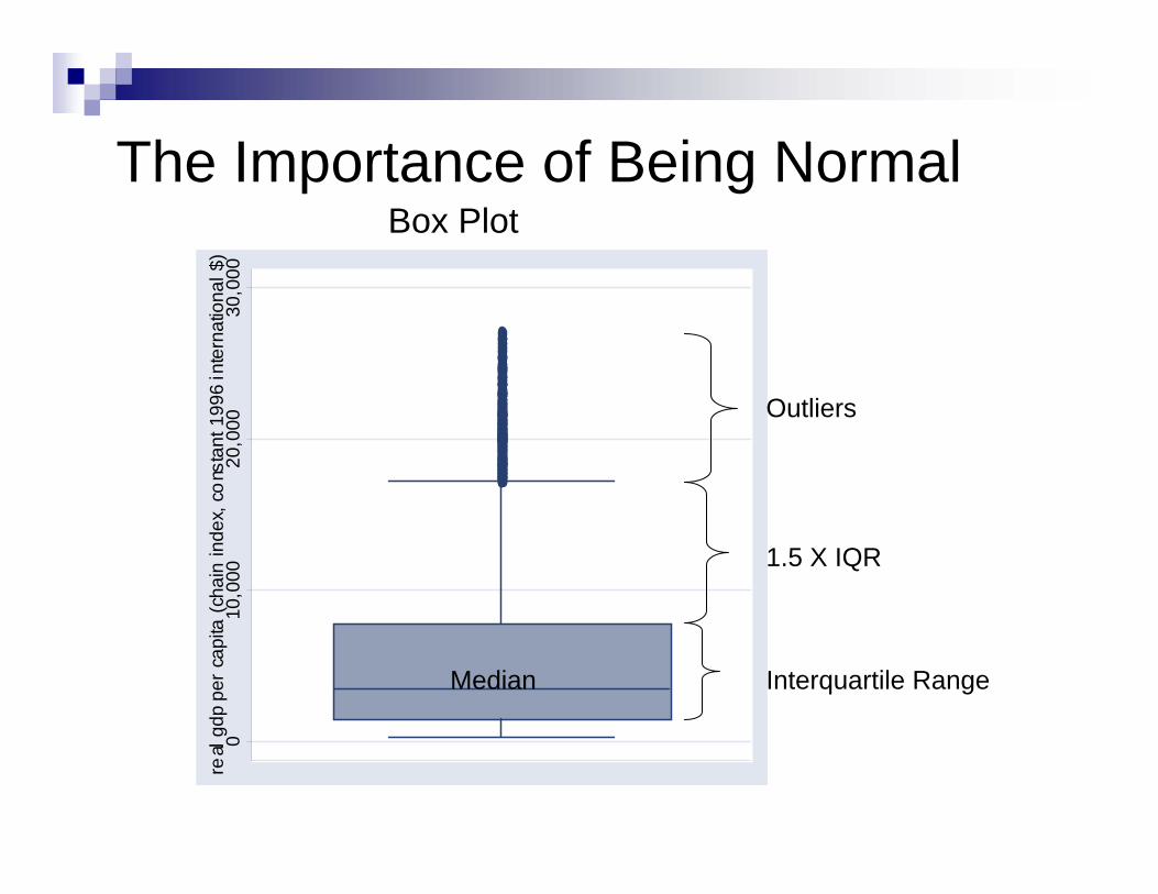
)Box Plot
Median
Outliers
Interquartile Range
1.5 X IQR
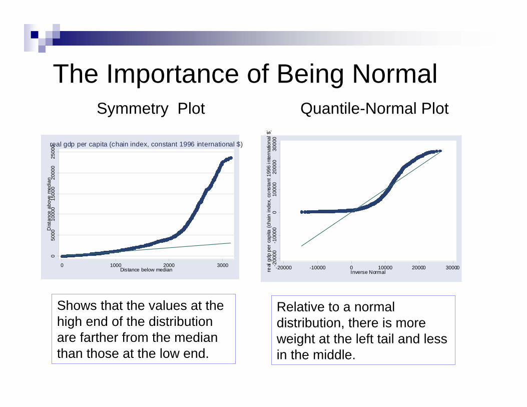
The Importance of Being NormalSymmetry Plot
050
0010
000
1500
020
000
2500
0D
ista
nce
abov
e m
edia
n
0 1000 2000 3000Distance below median
real gdp per capita (chain index, constant 1996 international $)
-200
00-1
0000
010
000
2000
030
000
real
gdp
per
capi
ta (c
hain
inde
x, co
nsta
nt 1
996
inte
rnat
iona
l $)-20000 -10000 0 10000 20000 30000
Inverse Normal
Quantile-Normal Plot
Shows that the values at the high end of the distribution are farther from the median than those at the low end.
Relative to a normal distribution, there is more weight at the left tail and less in the middle.
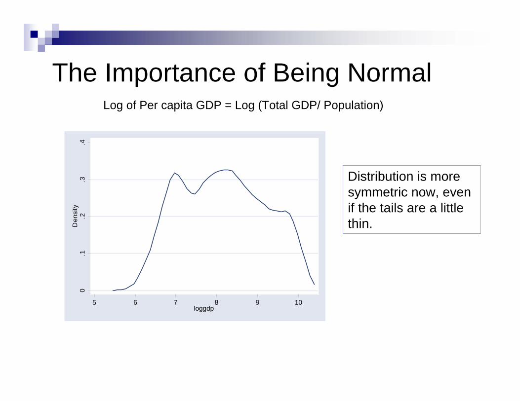
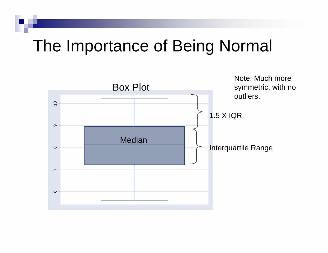
The Importance of Being NormalLog of Per capita GDP = Log (Total GDP/ Population)
0.1
.2.3
.4D
ensi
ty
5 6 7 8 9 10loggdp
Distribution is more symmetric now, even if the tails are a little thin.
67
89
10The Importance of Being Normal
Box Plot
Median
Note: Much more symmetric, with no outliers.
Interquartile Range
1.5 X IQR
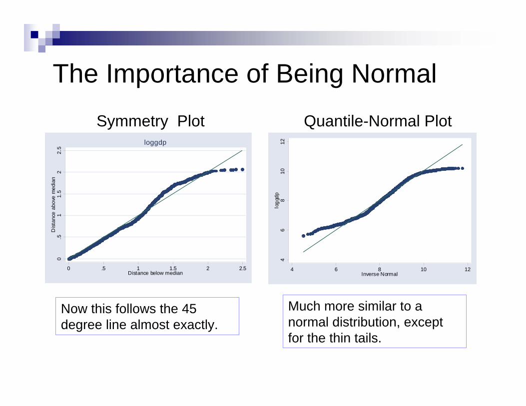
The Importance of Being NormalSymmetry Plot Quantile-Normal Plot
0.5
11.
52
2.5
Dis
tanc
e ab
ove
med
ian
0 .5 1 1.5 2 2.5Distance below median
loggdp
46
810
12lo
ggd
p4 6 8 10 12
Inverse Normal
Now this follows the 45 degree line almost exactly.
Much more similar to a normal distribution, except for the thin tails.
Inspecting Key Relationships-1
0-5
05
10Le
vel o
f Dem
ocra
cy
6 7 8 9 10Log of GDP per capita
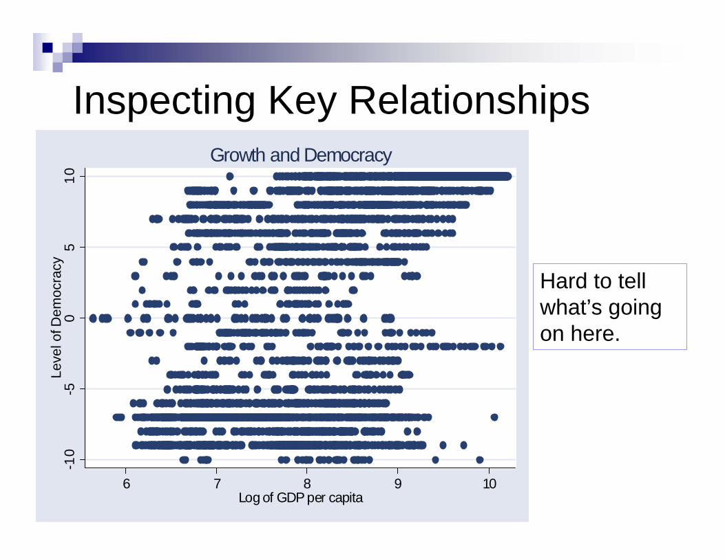
Growth and Democracy
Hard to tell what’s going on here.
Inspecting Key Relationships-1
0-5
05
10Le
vel o
f Dem
ocra
cy
6 7 8 9 10Log of GDP per capita
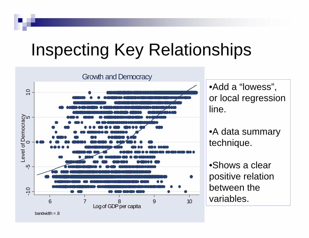
bandwidth = .8
Growth and Democracy•Add a “lowess”, or local regression line.
•A data summary technique.
•Shows a clear positive relation between the variables.
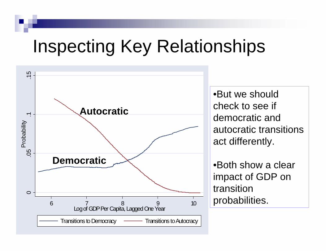
Inspecting Key Relationships0
.05
.1.1
5P
roba
bilit
y
6 7 8 9 10Log of GDP Per Capita, Lagged One Year
Transitions to Democracy Transitions to Autocracy
•But we should check to see if democratic and autocratic transitions act differently.
•Both show a clear impact of GDP on transition probabilities.
Democratic
Autocratic
Estimation TechniquesSay we decide to look at transitions:
Autocracy DemocracyDemocracy Autocracy
Then the dependent variable has only two values: Transition or No Transition
This type of “qualitative” dependent variable occurs often in social science:
Voting for a Republican or DemocratSupreme Court Decisions overrule or upholdYea and Nay votes when passing legislation, etc…
Appropriate estimation technique is “Probit”.Estimates nonlinear probabilities
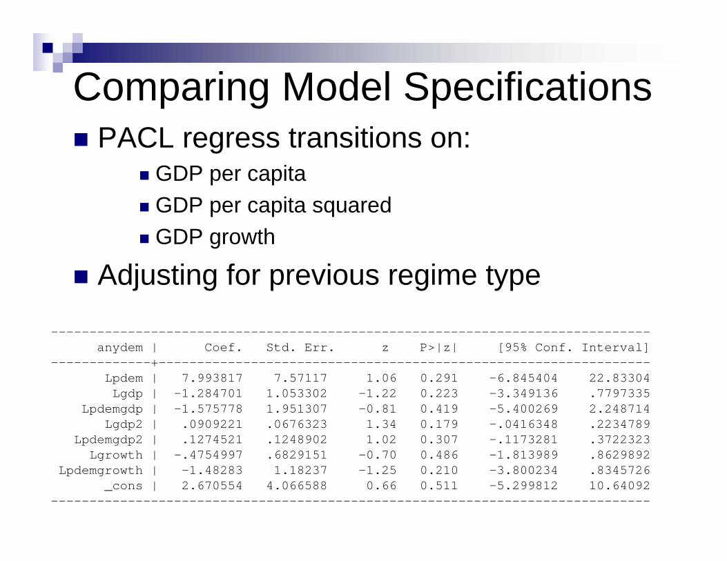
Comparing Model SpecificationsPACL regress transitions on:
GDP per capitaGDP per capita squaredGDP growth
Adjusting for previous regime type
------------------------------------------------------------------------------anydem | Coef. Std. Err. z P>|z| [95% Conf. Interval]
-------------+----------------------------------------------------------------Lpdem | 7.993817 7.57117 1.06 0.291 -6.845404 22.83304Lgdp | -1.284701 1.053302 -1.22 0.223 -3.349136 .7797335
Lpdemgdp | -1.575778 1.951307 -0.81 0.419 -5.400269 2.248714Lgdp2 | .0909221 .0676323 1.34 0.179 -.0416348 .2234789
Lpdemgdp2 | .1274521 .1248902 1.02 0.307 -.1173281 .3722323Lgrowth | -.4754997 .6829151 -0.70 0.486 -1.813989 .8629892
Lpdemgrowth | -1.48283 1.18237 -1.25 0.210 -3.800234 .8345726_cons | 2.670554 4.066588 0.66 0.511 -5.299812 10.64092
------------------------------------------------------------------------------
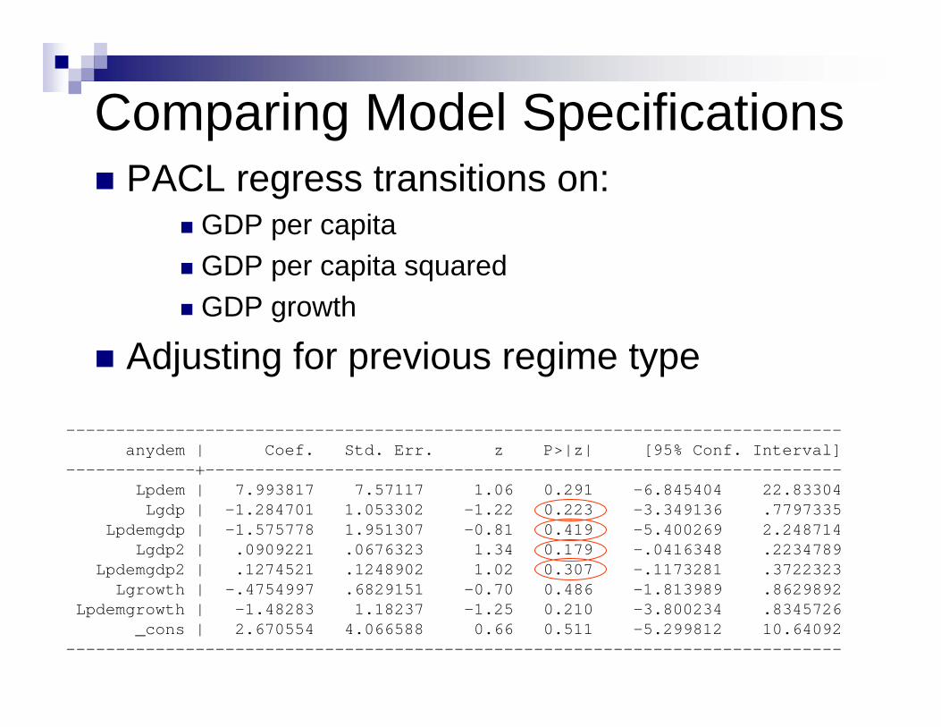
Comparing Model Specifications
------------------------------------------------------------------------------anydem | Coef. Std. Err. z P>|z| [95% Conf. Interval]
-------------+----------------------------------------------------------------Lpdem | 7.993817 7.57117 1.06 0.291 -6.845404 22.83304Lgdp | -1.284701 1.053302 -1.22 0.223 -3.349136 .7797335
Lpdemgdp | -1.575778 1.951307 -0.81 0.419 -5.400269 2.248714Lgdp2 | .0909221 .0676323 1.34 0.179 -.0416348 .2234789
Lpdemgdp2 | .1274521 .1248902 1.02 0.307 -.1173281 .3722323Lgrowth | -.4754997 .6829151 -0.70 0.486 -1.813989 .8629892
Lpdemgrowth | -1.48283 1.18237 -1.25 0.210 -3.800234 .8345726_cons | 2.670554 4.066588 0.66 0.511 -5.299812 10.64092
------------------------------------------------------------------------------
PACL regress transitions on:GDP per capitaGDP per capita squaredGDP growth
Adjusting for previous regime type
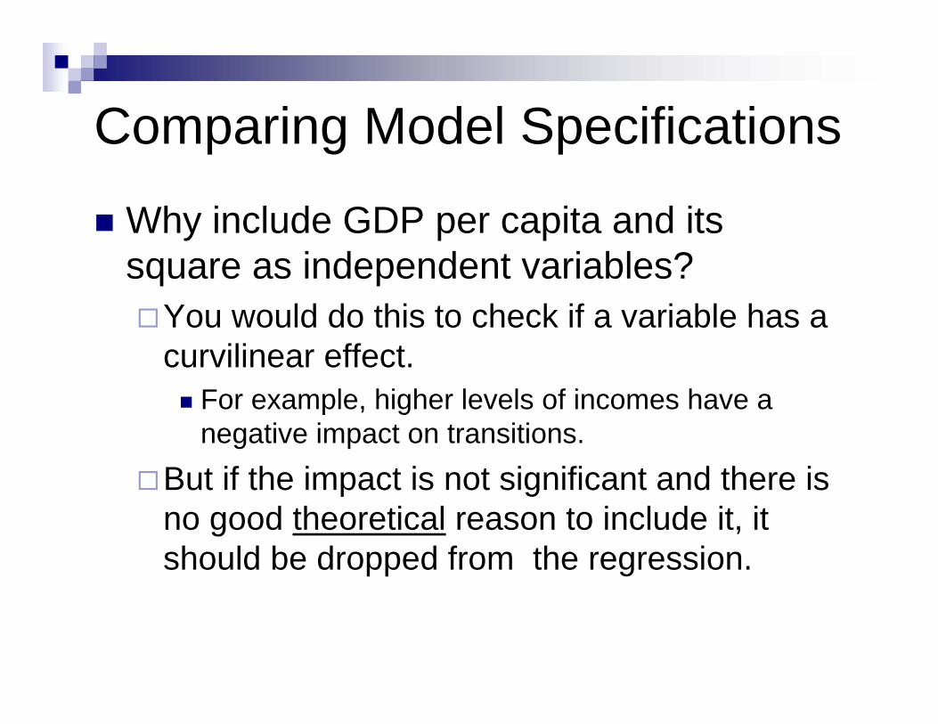
Why include GDP per capita and its square as independent variables?
You would do this to check if a variable has a curvilinear effect.
For example, higher levels of incomes have a negative impact on transitions.
But if the impact is not significant and there is no good theoretical reason to include it, it should be dropped from the regression.
Comparing Model Specifications
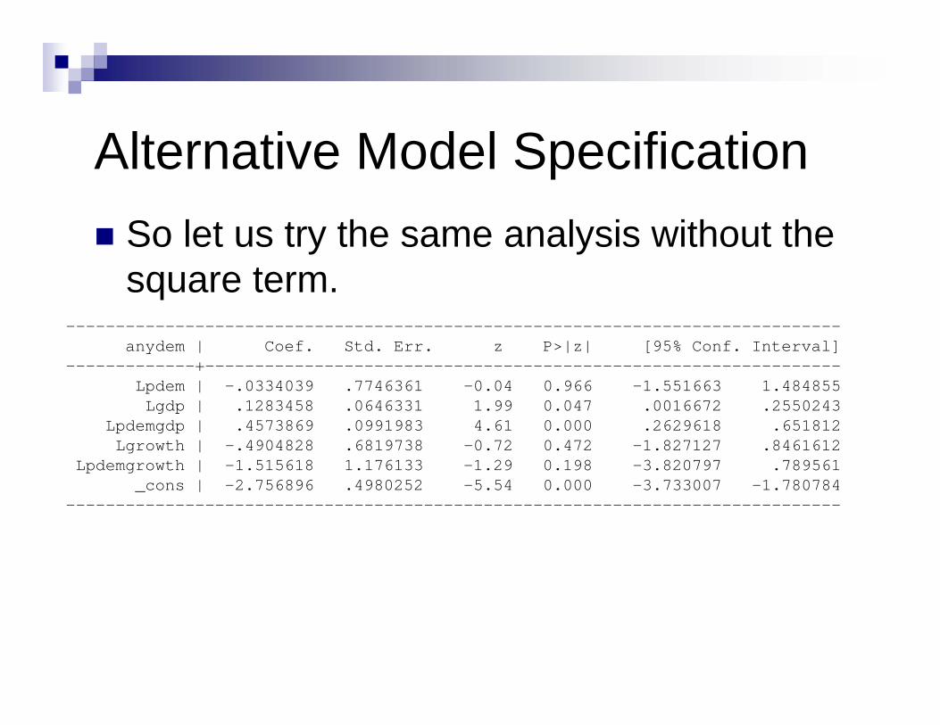
Alternative Model SpecificationSo let us try the same analysis without the square term.
------------------------------------------------------------------------------anydem | Coef. Std. Err. z P>|z| [95% Conf. Interval]
-------------+----------------------------------------------------------------Lpdem | -.0334039 .7746361 -0.04 0.966 -1.551663 1.484855Lgdp | .1283458 .0646331 1.99 0.047 .0016672 .2550243
Lpdemgdp | .4573869 .0991983 4.61 0.000 .2629618 .651812Lgrowth | -.4904828 .6819738 -0.72 0.472 -1.827127 .8461612
Lpdemgrowth | -1.515618 1.176133 -1.29 0.198 -3.820797 .789561_cons | -2.756896 .4980252 -5.54 0.000 -3.733007 -1.780784
------------------------------------------------------------------------------
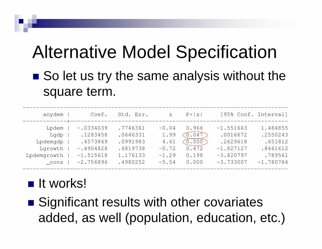
It works!Significant results with other covariates added, as well (population, education, etc.)
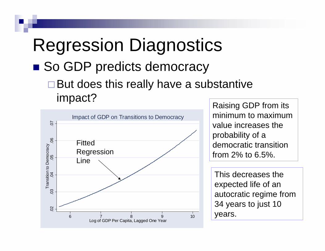
Regression DiagnosticsSo GDP predicts democracy
But does this really have a substantive impact?
.02
.03
.04
.05
.06
.07
Tran
sitio
n to
Dem
ocra
cy
6 7 8 9 10Log of GDP Per Capita, Lagged One Year
Impact of GDP on Transitions to Democracy
This decreases the expected life of an autocratic regime from 34 years to just 10 years.
FittedRegressionLine
Raising GDP from its minimum to maximum value increases the probability of a democratic transition from 2% to 6.5%.
0.0
5.1
.15
.2.2
5pa
ut
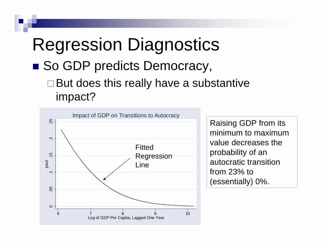
6 7 8 9 10Log of GDP Per Capita, Lagged One Year
Impact of GDP on Transitions to Autocracy
Regression DiagnosticsSo GDP predicts Democracy,
But does this really have a substantive impact?
Raising GDP from its minimum to maximum value decreases the probability of an autocratic transition from 23% to (essentially) 0%.
FittedRegressionLine
The End (Or the Beginning)What else could you do with this analysis?
Add more covariatesEducationPopulationResource Curse
Treat data differentlyUse entire democracy-autocracy scale, rather than dividing it into discrete categoriesTreat this as a survival problem
Others?
Class Organization
Text: Statistical SleuthWebsite: CourseWorksGrades:
Homework: 35%Midterm: 25%Final Paper and Presentation: 35%Participation: 5%