Statistical Shape Models

• Eigenpatches model regions – Assume shape is fixed– What if it isn’t?

• Faces with expression changes,

• organs in medical images etc

• Need a method of modelling shape and shape variation

Shape Models

• We will represent the shape using a set of points

• We will model the variation by computing the PDF of the distribution of shapes in a training set

• This allows us to generate new shapes similar to the training set

Building Models

• Require labelled training images– landmarks represent correspondences

Suitable Landmarks

• Define correspondences– Well defined corners

– `T’ junctions

– Easily located biological landmarks

– Use additional points along boundaries to define shape more accurately

Building Shape Models

• For each example

x = (x1,y1, … , xn, yn)T

Shape

• Need to model the variability in shape

• What is shape?– Geometric information that remains when

location, scale and rotational effects removed (Kendall)

Same Shape Different Shape

Shape

• More generally– Shape is the geometric information invariant to

a particular class of transformations

• Transformations:– Euclidean (translation + rotation)– Similarity (translation+rotation+scaling)– Affine

Shape

Shapes Euclidean Similarity Affine

Statistical Shape Models

• Given a set of shapes:

• Align shapes into common frame– Procrustes analysis

• Estimate shape distribution p(x)– Single gaussian often sufficient– Mixture models sometimes necessary

Aligning Two Shapes

• Procrustes analysis:– Find transformation which minimises

– Resulting shapes have • Identical CoG

• approximately the same scale and orientation

221 |)(| xx T

Aligning a Set of Shapes

• Generalised Procrustes Analysis– Find the transformations Ti which minimise

– Where

– Under the constraint that

2|)(| iiT xm

)(1

iiTn

xm

1|| m

Aligning Shapes : Algorithm

• Normalise all so CoG at origin, size=1

• Let

• Align each shape with m

• Re-calculate

• Normalise m to default size, orientation

• Repeat until convergence

1xm

)(1

iiTn

xm

Aligned Shapes

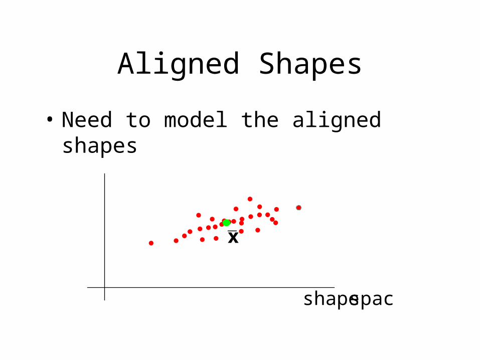
• Need to model the aligned shapes

x

space shape

Statistical Shape Models

• For shape synthesis– Parameterised model preferable

• For image matching we can get away with only knowing p(x)– Usually more efficient to reduce dimensionality

where possible

)(bx shapef Pbxx e.g.

Dimensionality Reduction

• Co-ords often correllated

• Nearby points move together

11bpxx

1b

xx

1p

Principal Component Analysis

• Compute eigenvectors of covariance,S

• Eigenvectors : main directions

• Eigenvalue : variance along eigenvector

1p2p

1 2

Dimensionality Reduction

• Data lies in subspace of reduced dim.

• However, for some t,

i

i

nnbb ppxx 11

tjb j if 0

t

) is of (Variance jjb

Building Shape Models

• Given aligned shapes, { }

• Apply PCA

• P – First t eigenvectors of covar. matrix

• b – Shape model parameters

ix

Pbxx

Hand shape model

• 72 points placed around boundary of hand– 18 hand outlines obtained by thresholding images of

hand on a white background

• Primary landmarks chosen at tips of fingers and joint between fingers– Other points placed equally between

1

23

4

5

6

Hand Shape Model

1 Varying b2 Varying b 3 Varying b

Face Shape Model

1 Varying b2 Varying b 3 Varying b

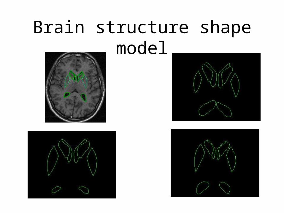
Brain structure shape model

Example : Hip Radiograph

11bpxx

1 1 33 1 b

Spine Model

Distribution of Parameters

• Learn p(b) from training set

• If x multivariate gaussian, then– b gaussian with diagonal covariance

• Can use mixture model for p(b)

)( 1 tb diag S

Conclusion

• We can build statistical models of shape change

• Require correspondences across training set

• Get compact model (few parameters)

• Next: Matching models to images