spectrum survey in urban environment: upc campus nord
TRANSCRIPT

Departament de Teoriadel Senyal i Comunicacions
UNIVERSITAT POLITÈCNICA DE CATALUNYA
Spectrum Survey in Urban Environment: UPC Campus Nord, Barcelona, Spain
Technical Report
December 2010
Miguel López‐Benítez and Fernando Casadevall
Mobile Communication Research Group (GRCM) Department of Signal Theory and Communications (TSC)
Universitat Politècnica de Catalunya (UPC)
http://www.tsc.upc.edu/grcm

Mobile Communication Research Group Technical Report Universitat Politècnica de Catalunya December 2010
Contents 1 INTRODUCTION ..................................................................................................................................... 3 2 MEASUREMENT SETUP......................................................................................................................... 4 2.1 ANTENNA SUBSYSTEM .......................................................................................................................... 4 2.2 RF SUBSYSTEM....................................................................................................................................... 5 2.3 SPECTRUM ANALYZER .......................................................................................................................... 7
3 MEASUREMENT SITE .......................................................................................................................... 10 3.1 MEASUREMENT SITE DESCRIPTION .................................................................................................... 10 3.2 MEASUREMENT SITE LOCATION......................................................................................................... 10 3.3 MEASUREMENT SITE VIEWS................................................................................................................ 11
4 MEASUREMENT RESULTS ................................................................................................................. 16 4.1 OCCUPANCY METRICS ........................................................................................................................ 16 4.2 OBTAINED RESULTS ............................................................................................................................ 16 4.3 SUMMARY OF SPECTRUM OCCUPANCY STATISTICS ........................................................................... 29 4.4 DISCUSSION ......................................................................................................................................... 32
5 CONCLUSIONS ...................................................................................................................................... 36
Page 2 of 37

Mobile Communication Research Group Technical Report Universitat Politècnica de Catalunya December 2010
1 Introduction
This document describes the spectrum occupancy measurements conducted by the Mobile Communication Research Group (GRCM) of the Technical University of Catalonia (Universitat Politècnica de Catalunya, UPC) in the UPC Campus Nord located in the city of Barcelona, Spain, in the frequency range from 75 MHz to 7075 MHz between November 2008 and February 2009.
This spectrum survey is motivated by the recent emergence of Dynamic Spectrum Access (DSA)
policies based on the Cognitive Radio (CR) technology. A proper understanding of current spectrum usage patterns can be very useful for policy makers to define adequate DSA policies and for the research community in general to identify appropriate frequency bands for the deployment of future DSA/CR networks. Some measurement campaigns covering both wide frequency ranges [1]–[6] and some specific licensed bands [7]–[11] have already been performed. The number of measured locations, however, can arguably be considered as insufficient. To enable a wide scale deployment, the DSA/CR technology cannot be based on the conclusions derived from studies conducted in a few geographical areas or under specific spectrum regulations. CR should take into account the possibility to operate under many different spectrum regulations and a wide variety of scenarios. Further spectrum measurements are therefore required, which motivates the spectrum survey reported in this document. The main goal of this spectrum measurement campaign is to identify spectrum bands with low occupancy levels that could be exploited for opportunistic use by DSA/CR networks. The obtained results demonstrate the availability of a significant amount of available spectrum.
Page 3 of 37

Mobile Communication Research Group Technical Report Universitat Politècnica de Catalunya December 2010
2 Measurement Setup The measurement equipment relies on a spectrum analyzer setup where different external
devices have been added in order to improve the detection capabilities of the system and hence obtain more accurate and reliable results. The design is composed of two broadband discone‐type antennas covering the frequency range from 75 to 7075 MHz, a Single‐Pole Double‐Throw (SPDT) switch to select the desired antenna, several filters to remove undesired overloading (FM) and out‐of‐band signals, a low‐noise pre‐amplifier to enhance the overall sensitivity and thus the ability to detect weak signals, and a high performance spectrum analyzer to record the spectral activity. A simplified scheme is shown in Figure 1. Moreover, Figure 2, Figure 3 and Figure 4 show the different parts of the measurement configuration, which are described in more detail in the following.
Discone antennaAOR DN753
75 – 3000 MHz
Spectrum analyzerAnritsu SpectrumMaster MS2721B9 kHz – 7.1 GHz
Discone antennaJXTXPZ-100800-P3000 – 7075 MHz
SPDT switchDC – 18 GHz
FM band stop filterRejection 20 – 35 dB
88 – 108 MHz
Low pass filterDC – 3000 MHz
High pass filter3000 – 7000 MHz
Low noise amplifierGain: 8 – 11.5 dB
Noise figure: 4 – 4.5 dB20 – 8000 MHz
Figure 1. Measurement setup (general scheme).
2.1 Antenna Subsystem
The antenna subsystem is shown in Figure 2. Two wideband discone‐type antennas are used to cover the frequency range from 75 to 7075 MHz. The first antenna (AOR DN753) is used between 75 and 3000 MHz, while the second antenna (A‐INFO JXTXPZ‐100800/P) is employed between 3000 and 7075 MHz. Discone antennas are wideband antennas with vertical polarization and omni‐directional receiving pattern in the horizontal plane. Even though some transmitters are horizontally polarized, they usually are high‐power stations (e.g., TV stations) that can be detected even with vertically polarized antennas. The exceptionally wideband coverage (allowing a reduced number of antennas in broadband spectrum studies) and the omni‐directional feature (allowing the detection of primary signals coming for any directions) make discone antennas an attractive choice for radio scanning and monitoring applications.
Page 4 of 37

Mobile Communication Research Group Technical Report Universitat Politècnica de Catalunya December 2010
Figure 2. Measurement setup (antenna subsystem).
2.2 RF Subsystem
The Radio Frequency (RF) subsystem is shown in Figure 3. This module performs antenna selection, filtering and amplification.
The desired antenna is selected by means of a SPDT switch (Mini‐Circuits SPDT Switch MSP2T‐18). An electromechanical switch has been selected because of its high isolation (90‐100 dB) and low insertion loss (0.1‐0.2 dB). When compared to other switch types, electromechanical switches in general provide slower switching times and shorter lifetimes. Nevertheless, this is not an issue since antenna switching is always performed off‐line by manually turning the switch on/off.
Page 5 of 37

Mobile Communication Research Group Technical Report Universitat Politècnica de Catalunya December 2010
To remove undesired signals, three filters are included. A band stop filter blocks signals in the frequency range of Frequency Modulation (FM) broadcast stations (87.5‐108 MHz). Usually, such stations are high power transmitters that may induce overload in the receiver thus degrading the receiver performance by an increased noise floor or by the presence of spurious signals, which inhibits the receiver’s ability to detect the presence of weak signals. Since the FM band is of presumably low interest for secondary use due to its usually high transmission power and expected high occupancy rate, a FM band stop filter (Mini‐Circuits NSBP‐108+) has been employed in order to remove FM signals and avoid overload problems, improving the detection of weak signals at other frequencies. Low pass (Mini‐Circuits VLF‐3000+) and high pass (Mini‐Circuits VHP‐26) filters have been used to remove out‐of‐band signals and reduce the potential inter‐modulation products.
To compensate for device and cable losses and increase the system sensitivity, a low‐noise pre‐
amplifier has been included. It is worth noting that higher amplification gains result in better sensitivity at the expense of reduced dynamic ranges. In broadband spectrum surveys, the measurement setup needs to be able to detect, over a wide range of frequencies, a large number of transmitters of the most diverse nature, from narrow band to wide band systems and from weak signals received near the noise floor to strong signals that may overload the receiving system. Therefore, the existing trade‐off between sensitivity and dynamic range needs to be taken into account. The selected mid‐gain amplifier (Mini‐Circuits ZX60‐8008E+) provides significant sensitivity improvements while guaranteeing the Spurious‐Free Dynamic Range (SFDR) required by the measured signals. It is worth noting that the employed spectrum analyzer includes a high‐gain built‐in amplifier. Nevertheless, the use of an additional external pre‐amplifier closer to the antenna system results in an improved overall noise figure (4‐5 dB lower than the case where only the internal pre‐amplifier is employed). For measurements below 3 GHz, where some overloading signals may be present, only the external amplifier is used. For measurements above 3 GHz, where the received powers are lower, both the external and the spectrum analyzer’s internal amplifier are employed.
Figure 3. Measurement setup (RF subsystem).
Page 6 of 37

Mobile Communication Research Group Technical Report Universitat Politècnica de Catalunya December 2010
2.3 Spectrum Analyzer An Anritsu Spectrum Master MS2721B high performance handheld spectrum analyzer is used to
provide power spectrum measurements and record the spectral activity over the complete frequency range. This spectrum analyzer provides a measurement range from 9 kHz to 7.1 GHz, low noise level (Displayed Average Noise Level lower than –163 dBm typical in a 1 Hz resolution bandwidth at 1 GHz) and a built‐in pre‐amplifier (≈25 dB gain) that facilitate the detection of weak signals, fast sweep speed automatically adjusted, and the possibility to connect an external USB storage device to save measurements for later data post‐processing. The spectrum analyzer provides a RJ45 Ethernet 10/100 Base T connection that enables controlling the instrument either directly (from a laptop or PC) or remotely (through a local area network or Internet). The spectrum analyzer also includes an external GPS sensor that allows including the coordinates of the current measurement location into the saved traces. Moreover the handheld, battery‐operated design simplifies the displacement of the equipment to different measurement locations.
Figure 4. Measurement setup (spectrum analyzer).
Since the different operating modes of spectrum analyzers can significantly alter the results of a measurement, proper parameter selection is crucial to produce valid and meaningful results. The different parameters of the spectrum analyzer have been set according to the basic principles of spectrum analysis [12][13] as well as some particular considerations specific to CR. Table 1 shows the main spectrum analyzer configuration parameters.
Page 7 of 37

Mobile Communication Research Group Technical Report Universitat Politècnica de Catalunya December 2010
Table 1. Spectrum analyzer configuration.
Parameter Value
Frequency range 75–3000 MHz 3000–7075 MHz
Frequency span 45–600 MHz
Frequency bin 81.8–1090.9 kHz
Resolution BandWidth (RBW) 10 kHz Frequency
Video BandWidth (VBW) 10 kHz
Measurement period 24 hours
Time
Sweep time Automatic
Built‐in pre‐amplifier Deactivated Activated
Reference level –20 dBm –50 dBm
Reference level offset 0 dB –20 dB
Scale 10 dB/division
Input attenuation 0 dB Amplitude
Detection type Average RMS detector
The measured frequency range (75‐7075 MHz) has been divided into 25 blocks with variable sizes
ranging from 45 MHz up to 600 MHz. Firstly, the division has been performed following the Spanish governmental spectrum allocations defined in [14]. As a result, no spectrum band in [14] has been split off when measuring. Another important aspect that has been taken into consideration when defining such bands is the relation between the frequency bin (distance between two consecutively measured frequency points) and the bandwidth of the signal being measured. Spectrum analyzers have a defined number of discrete frequency bins to store the results of a scan. In the case of the Anritsu MS2721B, the number of frequency points measured for a given range of frequencies (frequency span) is fixed and equal to 551 points per span. Therefore, the widths of the selected bands (frequency spans) have a direct impact on the frequency resolution of the measurements (frequency bins). It was observed that if the frequency bin is larger than the bandwidth of the signal being measured, spectrum occupancy is notably overestimated. On the other hand, occupancy estimation is reasonably accurate as long as the frequency bin size remains acceptably narrower than the signal bandwidth. Band division has therefore been performed satisfying this criterion as far as possible. For example, to measure the bands allocated to the Global System for Mobile communications (GSM) the selected frequency span (45 MHz) results in a frequency bin of 45 MHz / (551–1) = 81.8 kHz, which is notably narrower than the GSM signal bandwidth (200 kHz). Similarly, 727.3 kHz and 745.5 kHz bins have been employed to measure TeleVision (TV) bands (8 MHz signal bandwidth) and Universal Mobile Telecommunications System (UMTS) bands (5 MHz signal bandwidth), respectively.
The Resolution BandWidth (RBW) plays an important role in the obtained measurements. Narrowing the RBW increases the ability to resolve signals in frequency and reduces the noise floor (increasing the sensitivity) at the cost of an increased sweep time and hence a longer measurement period [12][13]. Taking into the characteristics of the measured bands, a 10‐kHz RBW has been selected as an adequate trade‐off between detection capabilities and required measurement time. The Video BandWidth (VBW) is a function that dates to analogical spectrum analyzers, but is now nearly obsolete. It can be used to reduce the effect of the noise on the displayed signal amplitude. When the
Page 8 of 37

Mobile Communication Research Group Technical Report Universitat Politècnica de Catalunya December 2010
VBW is narrower than the RBW, this filtering has the effect of reducing the peak‐to‐peak variations of the displayed signal, thus averaging noise without affecting any part of the trace that is already smooth (for example, a sinusoid displayed well above the noise level). With modern digital spectrum analyzers this smoothing effect can be achieved by means of trace averaging. To eliminate this analogical form of averaging, the VBW has been set equal to the RBW.
Each frequency band has been measured for an interrupted period of 24 hours. The spectrum analyzer’s built‐in pre‐amplifier has been used only above 3 GHz, resulting in a noise floor reduction of 20 dB. To simplify the data post‐processing, the noise floor values in the 75‐3000 MHz and 3000‐7075 MHz bands have been equalized by adding a 20‐dB offset to the power levels measured between 3000‐7075 MHz (reference level offset). The reference level (the maximum power of a signal that enters the spectrum analyzer and can be measured accurately) has then been adjusted according to the maximum power observed in each region, while the scale is adjusted according to the minimum signal level. No input attenuation has been employed. An average type detector has been used. This detector averages all the power levels sensed in one frequency bin in order to provide a representative power level for each measured frequency bin.
Page 9 of 37

Mobile Communication Research Group Technical Report Universitat Politècnica de Catalunya December 2010
3 Measurement Site
3.1 Measurement Site Description The measurement equipment employed in this survey was placed on the rooftop of the
department’s main building in urban Barcelona. The selected place is a strategic location with direct line‐of‐sight to several transmitting stations located a few tens or hundreds of meters away from the antenna and without buildings blocking the radio propagation. This strategic location enabled to accurately measure the spectral activity of, among others, TV and FM broadcast stations, several nearby base stations for cellular mobile communications and a military headquarter as well as some maritime and aeronautical transmitters due to the relative proximity to the harbor and the airport.
3.2 Measurement Site Location A map of the measurement location is shown in Figure 5. The measurement equipment was
placed in the rooftop of the building marked with a yellow circle (latitude: 41º 23’ 20” north; longitude: 2º 6’ 43” east; altitude: 175 meters).
Figure 5. UPC Campus Nord in urban Barcelona, Spain.
Page 10 of 37

Mobile Communication Research Group Technical Report Universitat Politècnica de Catalunya December 2010
3.3 Measurement Site Views
Figure 6 – Figure 13 show photographs taken from the measurement site. In Figure 6, it is possible to appreciate the presence of the Collserola Communication Tower,
from which TV signals are broadcasted along with some PMR/PAMR transmissions. Very powerful FM broadcasting signals are also transmitted from the same tower, which makes necessary the use of the FM band stop filter shown in Figure 1. A careful analysis of Figure 6 also reveals the presence of antennas for cellular mobile communication systems (left‐hand side).
Figure 7 shows the rooftop of a neighboring building, where some antennas can be identified as
well. Such antennas, however, are used for receiving purposes and do not lead to any interference issues with our measurement equipment. Some air‐conditioning systems are also observed in Figure 7, which might result in some low‐frequency noise, thus affecting the bands measured on the lowest region of spectrum. Given that measurements were performed during winter months, no noisy interference is expected from these devices.
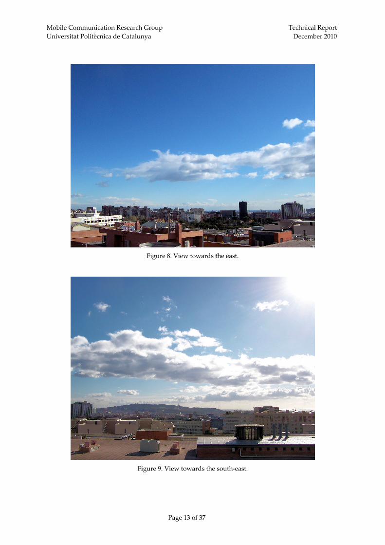
Figure 8 shows the view towards the city’s downtown, from where significant spectrum activity
levels can be expected at several spectrum bands. Dense urban areas are also included in the view of Figure 9, as well as the Montjuïc Communication tower, used by a cellular mobile operator, and from where relevant spectrum activities can also be expected.
Figure 10 points towards a nearby military headquarter, located right in front of the university
campus. At the bottom of the view, although not clearly appreciable, lays the control tower of the Barcelona’s airport with almost direct line‐of‐sight to the employed antenna system, which is also shown in the same figure. Direct line‐of‐sight, without blocking of the radio propagation, exists with aircrafts. The city’s harbor, located on the left‐hand side of the picture, can also be seen from the measurement location and spectrum activity is therefore also expected in maritime bands.
Figure 11 shows the rooftop of another neighboring building. Similar to Figure 7, several
antennas and air‐conditioning systems are also present, which are not expected to lead to interference issues for the reasons already explained. Parts of the military headquarter can also be observed, as well as antennas of cellular mobile communication systems located in the rooftops of some residential buildings. As a result, a clear appreciation of the spectrum activity in such bands is expected.
Figure 12 shows some antennas of cellular mobile communication systems, as it is the case of
Figure 11. Moreover, on the upper right‐hand side, a communication tower can also be appreciated. Such tower, however, is mainly used by parabolic antennas belonging to radio links. Given the high directivity of such antennas, no spectral activity is expected to be measured from this tower.
Finally, Figure 13 shows a view towards the nearby mountains, where no transmitters of special
interests can be identified.
Page 11 of 37

Mobile Communication Research Group Technical Report Universitat Politècnica de Catalunya December 2010
Figure 6. View towards the north.
Figure 7. View towards the north‐east.
Page 12 of 37
Mobile Communication Research Group Technical Report Universitat Politècnica de Catalunya December 2010
Figure 8. View towards the east.
Figure 9. View tow the south‐east. ards
Page 13 of 37

Mobile Communication Research Group Technical Report Universitat Politècnica de Catalunya December 2010
Figure 10. View towards the south.
Figure 11. View tow rds the south‐west. a
Page 14 of 37

Mobile Communication Research Group Technical Report Universitat Politècnica de Catalunya December 2010
Figure 12. View rds the west.
towa
Figure 13. View towards the north‐west.
Page 15 of 37
Mobile Communication Research Group Technical Report Universitat Politècnica de Catalunya December 2010
4 Measurement Results
4.1 Occupancy Metrics
Spectrum occupancy has been evaluated by means of three different occupancy metrics, which are shown in the figures presented in next subsection.
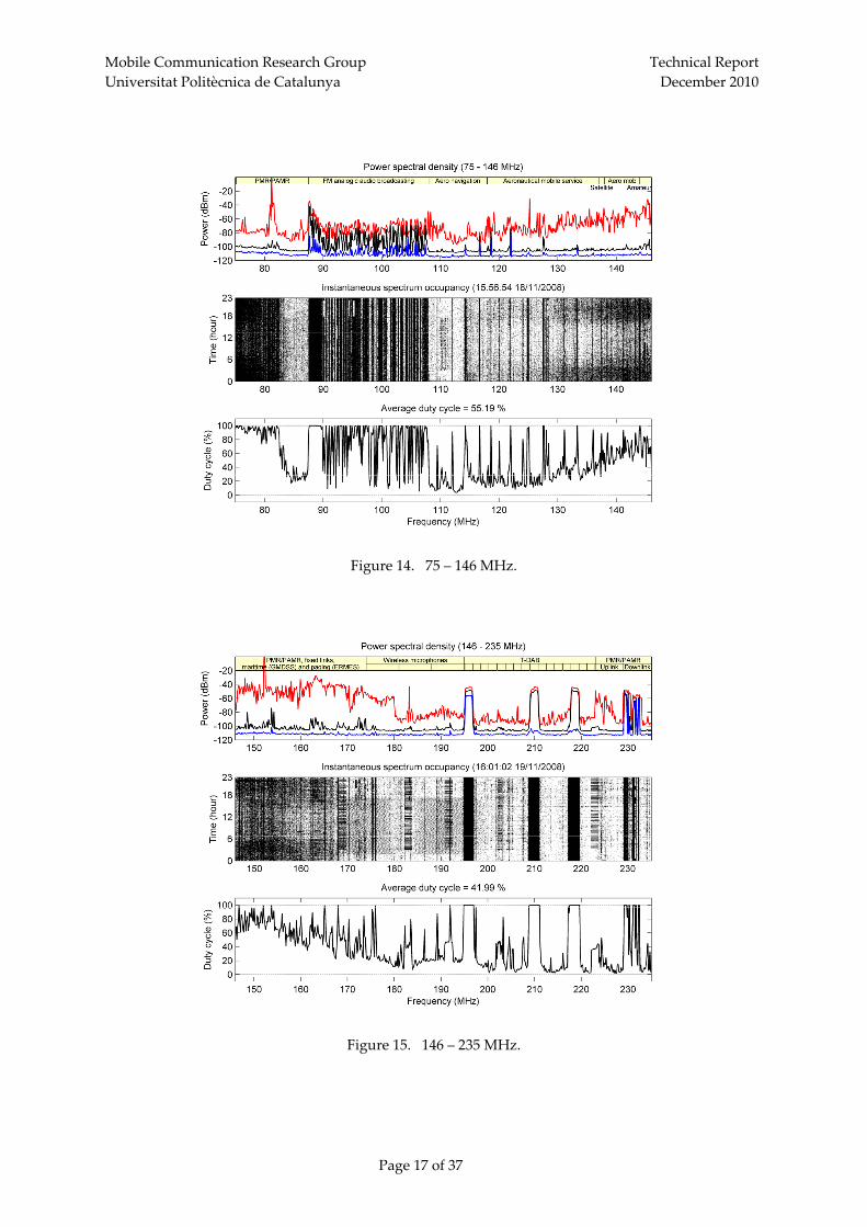
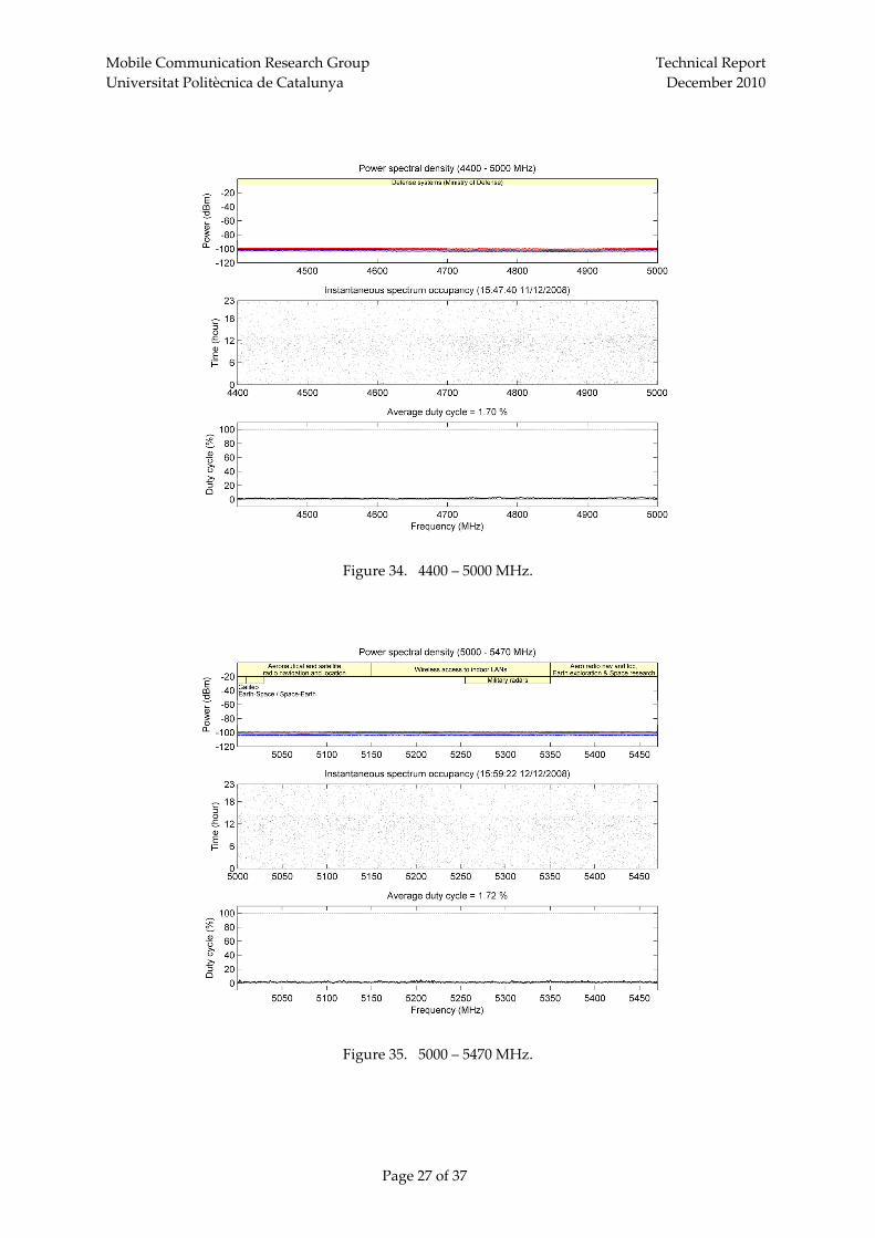
The first occupancy metric is Power Spectral Density (PSD), which is shown in the upper graph
of each figure in minimum, maximum and average values. When considered together, minimum, maximum and average PSD provide a simple characterization of the temporal behavior of a channel. For example, if the three PSD values are quite similar, it suggests a single transmitter that is always on, experiences a low level of fading and is probably not moving. At the other extreme, a large difference among minimum, maximum and average suggests a more intermittent use of spectrum.
The middle graph of each figure represents the instantaneous evolution of the temporal
spectrum occupancy. A black dot indicates that the corresponding frequency point was measured as busy at that time instant, while the white color means that the frequency point was measured as idle. To determine whether a frequency band is used by a licensed user, different sensing methods have been proposed in the literature [15]. They provide different tradeoffs between required sensing time, complexity and detection capabilities. Depending on how much information is available about the signal used by the licensed network different performances can be reached. However, in the most generic case no prior information is available. If only power measurements of the spectrum utilization are available, the energy detection method is the only possibility left. Due to its simplicity and relevance to the processing of power measurements, energy detection has been a preferred approach for many past spectrum studies and is also employed in this study. Energy detection compares the received signal energy in a certain frequency band to a predefined threshold. If the signal lies above the threshold the band is declared to be occupied by the primary network. Otherwise the band is supposed to be idle and could be employed by a CR network. The decision threshold employed in this study assumes a probability of false alarm equal to 1%. To compute such decision threshold, the system’s noise was measured by replacing the antennas with a 50 Ω matched load. The decision threshold at each frequency point was then fixed such that exactly 1% of the measured noise samples lied above the threshold, which implies a probability of false alarm of 1%. It is worth noting that the decision threshold obtained with this method is not constant since the system noise floor slightly increases with the frequency. Based on the obtained decision threshold, PSD samples above the threshold are assumed to be occupied; the rest of frequencies are assumed to be idle.
To more precisely quantify the detected primary activity, the lower graph of each figure shows
the duty cycle as a function of frequency. For each measured frequency point, the duty cycle is computed as the percentage of PSD samples, out of all the recorded PSD samples, that lied above the decision threshold and hence that were considered as samples of occupied channels. For a given frequency point, this metric represents the fraction of time that a frequency is considered to be busy. For a certain frequency band, the average duty cycle is computed by averaging the duty cycle of all the frequency points measured within the band.
4.2 Obtained Results
The following figures show the obtained spectrum occupancy results.
Page 16 of 37
Mobile Communication Research Group Technical Report Universitat Politècnica de Catalunya December 2010
Figure 14. 75 – 146 MHz.
Figure 15. 146 – 235 MHz.
Page 17 of 37

Mobile Communication Research Group Technical Report Universitat Politècnica de Catalunya December 2010
Figure 16. 235 – 317 MHz.
Figure 17. 317 – 400 MHz.
Page 18 of 37

Mobile Communication Research Group Technical Report Universitat Politècnica de Catalunya December 2010
Figure 18. 400 – 470 MHz.
Figure 19. 470 – 870 MHz.
Page 19 of 37

Mobile Communication Research Group Technical Report Universitat Politècnica de Catalunya December 2010
Figure 20. 870 – 915 MHz.
Figure 21. 915 – 960 MHz.
Page 20 of 37

Mobile Communication Research Group Technical Report Universitat Politècnica de Catalunya December 2010
Figure 22. 960 – 1155 MHz.
Figure 23. 1155 – 1350 MHz.
Page 21 of 37

Mobile Communication Research Group Technical Report Universitat Politècnica de Catalunya December 2010
Figure 24. 1350 – 1710 MHz.
Figure 25. 1710 – 1800 MHz.
Page 22 of 37

Mobile Communication Research Group Technical Report Universitat Politècnica de Catalunya December 2010
Figure 26. 1800 – 1880 MHz.
Figure 27. 1880 – 2290 MHz.
Page 23 of 37

Mobile Communication Research Group Technical Report Universitat Politècnica de Catalunya December 2010
Figure 28. 2290 – 2700 MHz.
Figure 29. 2700 – 3000 MHz.
Page 24 of 37

Mobile Communication Research Group Technical Report Universitat Politècnica de Catalunya December 2010
Figure 30. 3000 – 3400 MHz.
Figure 31. 3400 – 3600 MHz.
Page 25 of 37

Mobile Communication Research Group Technical Report Universitat Politècnica de Catalunya December 2010
Figure 32. 3600 – 4200 MHz.
Figure 33. 4200 – 4400 MHz.
Page 26 of 37
Mobile Communication Research Group Technical Report Universitat Politècnica de Catalunya December 2010
Figure 34. 4400 – 5000 MHz.
Figure 35. 5000 – 5470 MHz.
Page 27 of 37

Mobile Communication Research Group Technical Report Universitat Politècnica de Catalunya December 2010
Figure 36. 5470 – 5875 MHz.
Figure 37. 5875 – 6475 MHz.
Page 28 of 37

Mobile Communication Research Group Technical Report Universitat Politècnica de Catalunya December 2010
Figure 38. 6475 – 7075 MHz.
4.3 Summary of Spectrum Occupancy Statistics
Table 2 shows a summary of the obtained spectrum occupancy statistics, averaged over ≈ 1 GHz sub‐bands. A more detailed summary of the spectrum occupancy statistics is provided in Table 3, where the obtained results are summarized for each measured band. Figure 39 provides a graphical representation of the band by band average duty cycle statistics for the whole measurement range.
Table 2. Summary of spectrum occupancy averaged over sub‐bands.
Frequency
range (MHz) Average duty cycle
75 – 1000 42.00 %
1000 – 2000 13.30 % 31.02 %
2000 – 3000 3.73 %
3000 – 4000 4.01 %
4000 – 5000 1.63 %
5000 – 6000 1.98 %
6000 – 7075 1.78 %
2.75 %
17.78 %
Page 29 of 37

Mobile Communication Research Group Technical Report Universitat Politècnica de Catalunya December 2010
Table 3. Summary of spectrum occupancy in each band.
Start Freq (MHz)
Stop Freq (MHz)
Band width (MHz)
Spectrum band allocation Occupied spectrum
(MHz)
Averageoccupied
(%) 75.2 87.5 12.3 PMR/PAMR 8.59 69.83 87.5 108 20.5 FM analogical audio broadcasting 15.81 77.11 108 137 29 Aero radionavigation (ILS/VOR) 8.86 30.54 137 144 7 Aeronautical, maritime & satellite 4.37 62.40 144 146 2 Amateur 1.43 71.27 146 174 28 PMR/PAMR, fixed links, maritime (GMDSS), paging (ERMES) 16.86 60.21 174 195 21 Wireless microphones 6.22 29.61 195 223 28 DAB-T 10.66 38.06 223 235 12 PMR/PAMR 3.76 31.32 235 400 165 Defense systems (DoD) & TETRA 41.05 24.88 400 406 6 Satellite & ULP-AMI 0.74 12.36 406 430 24 PMR/PAMR (TETRA) 7.98 33.25 430 440 10 Amateur & ISM-433 (SRD) 2.90 28.97 440 470 30 PMR/PAMR (PMR 446 & TETRA) 9.28 30.93 470 862 392 DVB-T 321.75 82.08 862 868 6 Wireless microphones & RFID 4.01 66.85 868 870 2 SRD & alarms 0.52 26.06 870 876 6 PMR/PAMR (CT1-E cordless telephones & TETRA) UL 0.25 4.17 876 880 4 R-GSM 900 UL 0.06 1.39 880 915 35 E-GSM 900 UL 2.19 6.26 915 921 6 PMR/PAMR (CT1-E cordless telephones & TETRA) DL 0.05 0.86 921 925 4 R-GSM 900 DL 0.88 21.91 925 960 35 E-GSM 900 DL 33.72 96.33 960 1350 390 Aero and satellite radionavigation/location (GALILEO) 18.72 4.80 1350 1400 50 Defense systems (DoD) 0.54 1.08 1400 1427 27 Satellite 1.33 4.93 1427 1452 25 Point-to-point fixed links 2.25 8.99 1452 1492 40 Audio broadcasting (DAB-T & satellite) 1.66 4.15 1492 1517 25 Point-to-point fixed links 1.76 7.05 1517 1530 13 Defense systems (DoD) 0.37 2.83 1530 1559 29 Satellite (MSS) 0.69 2.37 1559 1610 51 Aero and satellite radionavigation/location (GPS/GALILEO/GLONASS) 3.64 7.14 1610 1675 65 Satellite (S-PCS) & SAP/SAB point-to-point audio links 8.71 13.40 1675 1710 35 Defense systems (DoD) 1.03 2.94 1710 1785 75 DCS 1800 UL 0.44 0.59 1785 1800 15 Radio microphones 0.08 0.52 1800 1805 5 Harmonized uses 0.05 0.98 1805 1880 75 DCS 1800 DL 44.12 58.82 1880 1900 20 DECT 2.10 10.50 1900 1920 20 UMTS FDD 0.13 0.64 1920 1980 60 UMTS FDD UL 0.38 0.64 1980 2010 30 UMTS satellite component 0.16 0.53 2010 2025 15 UMTS TDD 0.08 0.51 2025 2110 85 Point-to-point fixed links 0.44 0.52 2110 2170 60 UMTS FDD DL 34.16 56.93 2170 2200 30 UMTS satellite component 0.87 2.90 2200 2290 90 Point-to-point fixed links 0.52 0.58 2290 2300 10 Land mobile 0.05 0.46 2300 2500 200 ENG, RFID & ISM 2450 1.08 0.54 2500 2690 190 UMTS extension 1.16 0.61 2690 2700 10 Satellite 0.05 0.45 2700 2900 200 Military radars 1.50 0.75 2900 3100 200 Radionavigation/location (defense systems) 1.72 0.86 3100 3400 300 Military radars 1.80 0.60 3400 3600 200 BWA (MMDS) and military radars 18.36 9.18 3600 4200 600 Analogic links for telephony and TV 8.64 1.44 4200 4400 200 Aeronautical radionavigation 2.68 1.34 4400 5000 600 Defense systems (DoD) 10.14 1.69 5000 5150 150 Aero and satellite radionavigation/location (GALILEO) 2.54 1.69 5150 5350 200 Wireless access to indoor LANs 3.32 1.66 5350 5470 120 Radiolocation, aero radionavigation, Earth exploration & space research 2.22 1.85 5470 5725 255 Wireless access to indoor/outdoor LANs 5.53 2.17 5725 5875 150 ISM 5800 (wideband data, SRD, RFID & RTTT) 3.54 2.36 5875 7075 1200 Fixed links 21.60 1.80
Page 30 of 37

Mobile Communication Research Group Technical Report Universitat Politècnica de Catalunya December 2010
Figure 39. Band by band average duty cycle statistics for the whole m
easurement range.
Page 31 of 37

Mobile Communication Research Group Technical Report Universitat Politècnica de Catalunya December 2010
4.4 Discussion Spectrum experiences a relatively moderate use below 1 GHz and a low usage between 1 and 2
GHz, while remains mostly underutilized between 2 and 7 GHz (with some clear exceptions that will be discussed later on). In fact, while the average duty cycle between 75 and 2000 MHz is 31.02%, the value for this parameter between 2000 and 7075 MHz is only 2.75%, as shown in Table 2. The overall average duty cycle over the whole frequency range considered in this study is only 17.78%, which reveals the existence of significant amounts of unused spectrum that could potentially be exploited by future CR networks. Although these results clearly indicate low spectrum utilization levels, they do not provide a clear picture of how spectrum is used in different frequency bands allocated to different specific services. Therefore, in the following we discuss in detail the spectrum usage in some allocated bands of interest.
Although the highest spectral activity is observed below 1 GHz, some opportunities for CR
networks can still be found in this frequency range, even in those bands with the highest observed average duty cycles. For example, the frequency band 470‐862 MHz (depicted in Figure 40), which is allocated to analogical1 and digital terrestrial TV in Spain, shows an average duty cycle of 82.08%, one the highest values observed in this study. Although the sub‐band 830‐862 MHz (exclusively reserved for digital TV systems when measurements were performed) exhibits an intensive usage of nearly 100% that precludes any CR applications, the rest of the band between 470 and 830 MHz (allocated to both analogical and digital TV systems) shows some spectrum white spaces. Notice that occupied TV channels show a duty cycle of about 100%, i.e. continuous broadcasting, which impedes temporary opportunistic usage of those channels. Only one channel out of all the TV channels received at our measurement location (channel 38, 606‐614 MHz) was disconnected during a short period in the night, which might be due to maintenance operations since this behavior was not observed in some previous experiments. In general, occupied TV channels show an average duty cycle of 100%. Spectrum opportunities in this band usually come from TV channels that are received with very weak signal levels. In our case, the measured average duty cycle between 470 and 830 MHz was 80.49%, meaning that one fifth of the TV band (approximately 80 MHz) can be considered as idle due to the weak reception of the signals broadcasted from distant TV stations. Therefore, although the TV band appears as considerably populated in our study, it provides some interesting opportunities for secondary usage. Nowadays, with the transition towards digital TV, higher amounts of free bandwidth are available2 (e.g., measurements performed on November 2010 indicated an average duty cycle within the same frequency range of approximately 60%).
Another interesting case below 1 GHz is observed in the frequency bands allocated to the Global
System for Mobile communications (GSM). The Enhanced GSM (E‐GSM) 900 system operates in the 880‐915 MHz (uplink) and 925‐960 MHz (downlink) bands as shown in Figure 41. The uplink band appears as a potential candidate for CR applications with an average duty cycle equal to 6.26%. However, in this case it is important to highlight that the low activity recorded in this band does not necessarily imply that it could be used by CR networks. As a matter of fact, the maximum PSD observed in Figure 41 reaches significant values, revealing the presence of primary signals in uplink. The considerably higher activity in downlink (96.33%) and the fact that GSM is based on Frequency‐Division Duplex (FDD) suggest that the actual usage of the uplink band might be higher than the activity level recorded at the considered measurement location. The unbalanced occupancy patterns between uplink and downlink in Figure 41 can be explained as follows. First, the transmission power
1 At the moment of performing the field measurements, analogical TV stations were still allowed to operate in TV bands in Spain and, in fact, some of them can be identified in Figure 40. 2 An 8‐MHz radio frequency channel can accommodate one analogical TV transmission and four digital TV transmissions. As result of the transition towards digital TV, some radio frequency channels have been released recently.
Page 32 of 37

Mobile Communication Research Group Technical Report Universitat Politècnica de Catalunya December 2010
of GSM base stations is considerably higher than that of cellular phones. Therefore, the presence of GSM downlink signals can be more easily detected. Moreover, the antenna employed in our study was placed on the roof of a building with direct line‐of‐sight to several nearby base stations, which enabled us to accurately measure the high spectral activity of the downlink. On the other hand, the low usage observed in the uplink may be due to the usually low transmission power of cellular phones and the resulting weak uplink signal received at the antenna. The detection of such signals might be hindered by the fact that cellular phones usually operate at the ground level or low altitudes and usually have no direct line‐of‐sight neither with the serving base station nor the antenna employed in our study, which makes more difficult to detect the uplink activity. In fact, the maximum PSD observed in uplink in Figure 41 may be due to phone calls from nearby locations, e.g. the upper floors of the building. Therefore, from the obtained results we cannot conclude low activity levels in the E‐GSM 900 uplink.
In the lower spectrum bands 75‐235 MHz, 235‐400 MHz and 400‐470 MHz, low to moderate
average duty cycles of 48.59%, 24.88% and 29.85% are observed respectively. These bands are populated by a wide variety of narrowband systems, including Professional Mobile Radio/Public Access Mobile Radio (PMR/PAMR) systems (75.2‐87.5 MHz, 223‐235 MHz, 406‐430 MHz and 440‐470 MHz), FM analogical audio broadcasting (87.5‐108 MHz), aeronautical radio navigation and communication systems, maritime systems (GMDSS), paging systems (ERMES) and fixed links (108‐174 MHz), audio applications such as wireless microphones (174‐195 MHz) and Digital Audio Broadcasting (DAB) systems (195‐223 MHz), satellite systems (137‐138 MHz and 400‐406 MHz) and amateur systems (144‐146 MHz and 430‐440 MHz). Although these bands exhibit low to moderate average duty cycles, the free spectrum gaps found in this region of the spectrum are of considerably narrow bandwidths due to the narrowband nature of the systems operating within these bands. Moreover, the whole band from 235 to 400 MHz is exclusively reserved for security services and defense systems of the Spanish Ministry of Defense, which in principle precludes the use of such spectrum bands for CR applications. Other bands below 1 GHz with low or moderate levels of activity but narrower available free bandwidths are those assigned to wireless microphones and RFID (862‐870 MHz), CT1 cordless phones (870‐871 and 915‐916 MHz), cellular access rural telephony (874‐876 and 919‐921 MHz) and R‐GSM 900 (876‐880 and 921‐925 MHz).
Between 1 and 2 GHz, spectrum is subject to a low level of utilization, while remains mostly
unused between 2 and 7 GHz. Above 1 GHz the highest spectrum usage is observed for the bands allocated to the Digital Cellular System (DCS) 1800 operating at 1710‐1785 MHz and 1805‐1880 MHz (Figure 42), the Universal Mobile Telecommunication System (UMTS) operating at 1920‐1980 MHz and 2110‐2170 MHz (Figure 43), and Broadband Wireless Access (BWA) systems operating in the 3.4‐3.6 GHz band between 3520 and 3560 MHz (Figure 44).
Notice that the differences between uplink and downlink usage patterns that were appreciated
for E‐GSM 900 are also observed for DCS 1800 and UMTS. In the case of DCS 1800 the differences are more accentuated due to the fact that mobile stations in DCS 1800 have lower transmission powers than in GSM 900, which results in a reduced occupancy in the uplink. In the case of UMTS the difference is higher due to the spread spectrum nature of the Wideband Code Division Multiple Ac‐cess (WCDMA) radio technology employed by UMTS. WCDMA signals are modulated over large bandwidths, which results in very low transmission powers. Such signals are difficult to detect with spectrum analyzers. As a result, a very low activity was recorded in UMTS uplink. Although DCS 1800 and UMTS show higher levels of occupancy in downlink (58.82% and 56.93% respectively), these bands also provide some opportunities for secondary access. In the case of DCS 1800 some portions of the downlink band show a well defined periodic usage pattern, as it is illustrated in Figure 45 where the average duty cycle computed over 1‐hour periods is shown. Such temporal patterns could be exploited by some secondary CR applications by accessing spectrum during low‐occupancy periods.
Page 33 of 37

Mobile Communication Research Group Technical Report Universitat Politècnica de Catalunya December 2010
In the case of UMTS, spectrum opportunities are due to several 5‐MHz channels that appear to be unoccupied. Moreover, the UMTS bands reserved for the Time Division Duplex (TDD) component (1900‐1920 and 2010‐2025 MHz), the satellite component (1980‐2010 MHz and 2170‐2200 MHz) and extension (2500‐2690 MHz) are not used.
Although the highest activity above 1 GHz is observed for DCS 1800, UMTS and BWA systems,
some other bands are also clearly busy but at lower occupancy rates, which in principle offers additional opportunities for CR applications. Some examples are the 1400‐1710 MHz band, allocated to different wireless systems such as Satellite Personal Communication Systems (S‐PCS) as well as aeronautical radio navigation, audio broadcasting and defense systems, or the 3800‐4200 MHz band, allocated to analogical links for telephony.
Finally, it is worth noting that some spectrum bands appear as unoccupied when judged by their
average duty cycles. Nevertheless, the maximum PSD reveals that some primary users, although difficult to detect, are present in such bands. Some examples are the uplink bands for mobile communications, the 2400‐2500 MHz band (ISM‐2450), the 2900‐3100 MHz band (radio navigation and location systems) and the 4200‐4400 MHz band (allocated to aeronautical radio navigation).
Page 34 of 37

Mobile Communication Research Group Technical Report Universitat Politècnica de Catalunya December 2010
500 550 600 650 700 750 800 850−120−100−80−60−40−20
Pow
er (
dBm
)Power spectral density (470 − 862 MHz)
Analogic and digital TV (channels 21−65) Dig TV(66−69)
Tim
e (h
our)
Instantaneous spectrum occupancy
500 550 600 650 700 750 800 8500
6
12
18
24
500 550 600 650 700 750 800 8500
20406080
100
Frequency (MHz)
Dut
y cy
cle
(%)
Average duty cycle = 82.08 %
Figure 40. Spectrum occupancy for TV band
(470‐862 MHz).
870 880 890 900 910 920 930 940 950 960−120−100−80−60−40−20
Pow
er (
dBm
)
Power spectral density (870 − 960 MHz)
PMRR−GSM900 UL
E−GSM 900 uplink PMRR−GSM900 DL
E−GSM 900 downlink
Tim
e (h
our)
Instantaneous spectrum occupancy
870 880 890 900 910 920 930 940 950 9600
6
12
18
24
870 880 890 900 910 920 930 940 950 9600
20406080
100
Frequency (MHz)
Dut
y cy
cle
(%)
Average duty cycle = 41.13 %
Figure 41. Spectrum occupancy for E‐GSM 900
(870‐960 MHz).
1720 1740 1760 1780 1800 1820 1840 1860 1880−120−100−80−60−40−20
Pow
er (
dBm
)
Power spectral density (1710 − 1880 MHz)
DCS 1800 uplink DCS 1800 downlink
Tim
e (h
our)
Instantaneous spectrum occupancy
1720 1740 1760 1780 1800 1820 1840 1860 18800
6
12
18
24
1720 1740 1760 1780 1800 1820 1840 1860 18800
20406080
100
Frequency (MHz)
Dut
y cy
cle
(%)
Average duty cycle = 27.89 %
Figure 42. Spectrum occupancy for DCS 1800
(1710‐1880 MHz).
1900 1950 2000 2050 2100 2150 2200 2250−120−100−80−60−40−20
Pow
er (
dBm
)Power spectral density (1880 − 2290 MHz)
DE
CT
UM
TS
TD
D
UMTS FDD UL
UM
TS
sat
UM
TS
TD
D
Fixed links UMTS FDD DL
UM
TS
sat
Fixed linksT
ime
(hou
r)
Instantaneous spectrum occupancy
1900 1950 2000 2050 2100 2150 2200 22500
6
12
18
24
1900 1950 2000 2050 2100 2150 2200 22500
20406080
100
Frequency (MHz)
Dut
y cy
cle
(%)
Average duty cycle = 9.56 %
Figure 43. Spectrum occupancy for UMTS
(1880‐2290 MHz).
3400 3450 3500 3550 3600−120−100−80−60−40−20
Pow
er (
dBm
)
Power spectral density (3400 − 3600 MHz)
BWA (MMDS) and military radars
BWA systemsMilitary radars
Tim
e (h
our)
Instantaneous spectrum occupancy
3400 3450 3500 3550 36000
6
12
18
24
3400 3450 3500 3550 36000
20406080
100
Frequency (MHz)
Dut
y cy
cle
(%)
Average duty cycle = 9.20 %
Figure 44. Spectrum occupancy for BWA
(3400‐3600 MHz).
1865
1870
1875 15:32
21:32
3:32
9:32
0
20
40
60
80
100
Time (hh:mm)
Traffic channels
Broadcast channel
Frequency (MHz)
Avera
ge d
uty
cycle
per
hour
(%)
Figure 45. Average duty cycle per hour for
DCS 1800 (1862.5 – 1875.5 MHz).
Page 35 of 37

Mobile Communication Research Group Technical Report Universitat Politècnica de Catalunya December 2010
5 Conclusions Spectrum experiences a relatively moderate use below 1 GHz and a low usage between 1 and 2
GHz, while remains mostly underutilized between 2 and 7 GHz. In fact, while the average duty cycle between 75 and 2000 MHz is 31.02%, the value for this parameter between 2000 and 7075 MHz is only 2.75%. The overall average duty cycle over the whole frequency range considered in this study is only 17.78%, which reveals the existence of significant amounts of unused spectrum that could potentially be exploited by future DSA/CR networks.
The obtained results demonstrate that some spectrum bands are subject to intensive usage while
some others show moderate utilization levels, are sparsely used and, in some cases, are not used at all. The highest occupancy rates were observed for bands allocated to broadcast services (TV as well as analogical and digital audio), followed by digital cellular services such as PMR/PAMR, paging, and mobile cellular communications (E‐GSM 900, DCS 1800 and UMTS) among others. Other services and applications, e.g. aeronautical radio navigation and location or defense systems, show different occupancy rates depending on the particular allocated band.
Most of spectrum offers possibilities for secondary DSA/CR usage, even those bands with the
highest observed activity levels in terms of average duty cycle. Nevertheless, it is worth highlighting that the average duty cycle by itself is not a sufficient statistic to declare a spectrum band as idle. Indeed, the maximum PSD of some portions of the spectrum reveals that some allocated frequency bands with approximately null average duty cycles are actually being occupied by some active primary systems. This issue should carefully be taken into account when selecting frequency bands for potential DSA/CR applications. For that reason, a more detailed study taking into account the administrative division of the spectrum in Spain (Cuadro Nacional de Assignación de Frecuencias, CNAF [14]) is being carried out. The empirical spectrum occupancy data obtained is allocated in a data base that can be publicly accessed via web at the following URL: http://spes.upc.edu.
Page 36 of 37

Mobile Communication Research Group Technical Report Universitat Politècnica de Catalunya December 2010
Page 37 of 37
References [1] F. H. Sanders, “Broadband spectrum surveys in Denver, CO, San Diego, CA, and Los Angeles,
CA: methodology, analysis, and comparative results,” in Proc. 1998 IEEE International Symposium on Electromagnetic Compatibility, Aug 1998, vol. 2, pp. 988–993.
[2] M. A. McHenry et al., “Spectrum occupancy measurements,” Shared Spectrum Company, Tech. reports (Jan 2004 – Aug 2005). Available: http://www.sharedspectrum.com.
[3] A. Petrin, P. G. Steffes, “Analysis and comparison of spectrum measurements performed in urban and rural areas to determine the total amount of spectrum usage,” in Proc. International Symposium on Advanced Radio Technologies (ISART 2005), Mar 2005, pp. 9–12.
[4] R. I. C. Chiang, G. B. Rowe, K. W. Sowerby, “A quantitative analysis of spectral occupancy measurements for cognitive radio,” in Proc. IEEE 65th Vehicular Technology Conference (VTC 2007‐Spring), Apr 2007, pp. 3016–3020.
[5] M. Wellens, J. Wu, P. Mähönen, “Evaluation of spectrum occupancy in indoor and outdoor scenario in the context of cognitive radio,” in Proc. Second International Conference on Cognitive Radio Oriented Wireless Networks and Communications (CrowCom 2007), Aug 2007, pp. 1‐8.
[6] M. H. Islam et al., “Spectrum Survey in Singapore: Occupancy Measurements and Analyses,” in Proc. 3rd International Conference on Cognitive Radio Oriented Wireless Networks and Communications (CrownCom 2008), May 2008, pp. 1–7.
[7] P. G. Steffes, A. J. Petrin, “Study of spectrum usage and potential interference to passive remote sensing activities in the 4.5 cm and 21 cm bands,” in Proc. IEEE International Geoscience and Remote Sensing Symposium (IGARSS 2004), Sep 2004, vol. 3, pp. 1679–1682.
[8] J. Do, D. M. Akos, P. K. Enge, “L and S bands spectrum survey in the San Francisco bay area,” in Proc. Position Location and Navigation Symposium (PLANS 2004), Apr 2004, pp. 566–572.
[9] M. Biggs, A. Henley, T. Clarkson, “Occupancy analysis of the 2.4 GHz ISM band,” IEE Proc. on Comms, Oct 2004, vol. 151, nº 5, pp. 481–488.
[10] S. W. Ellingson, “Spectral occupancy at VHF: implications for frequency‐agile cognitive radios,” in Proc. IEEE 62nd Vehicular Technology Conference (VTC 2005‐Fall), Sep 2008, vol. 2, pp. 1379–1382.
[11] S. D. Jones, E. Jung, X. Liu, N. Merheb, I.‐J. Wang, “Characterization of spectrum activities in the U.S. public safety band for opportunistic spectrum access,” in Proc. 2nd IEEE International Symposium on New Frontiers in Dynamic Spectrum Access Networks (DySPAN 2007), Apr 2007, pp. 137–146.
[12] Agilent, Application note 150: Spectrum analysis basics, available at: http://www.agilent.com. [13] Agilent, Application note 1286‐1: 8 Hints for Better Spectrum Analysis, available at:
http://www.agilent.com. [14] Secretaría de Estado de Telecomunicaciones y para la Sociedad de la Información (State Agency
for Telecommunications and Information Society), “Cuadro Nacional de Atribución de Frecuencias (Table of National Frequency Allocations),” Spanish Ministry of Industry, Tourism and Commerce, Tech. Rep., Nov. 2007.
[15] T. Yucek, H. Arslan, “A survey of spectrum sensing algorithms for cognitive radio applications,” IEEE Communication Surveys and Tutorials, vol. 11, no. 1, pp. 116–130, First Quarter 2009.