source apportionment of submicron organic aerosols at an urban

Atmos. Chem. Phys., 7, 1503–1522, 2007www.atmos-chem-phys.net/7/1503/2007/© Author(s) 2007. This work is licensedunder a Creative Commons License.

AtmosphericChemistry

and Physics

Source apportionment of submicron organic aerosols at an urbansite by factor analytical modelling of aerosol mass spectra

V. A. Lanz1, M. R. Alfarra 2, U. Baltensperger2, B. Buchmann1, C. Hueglin1, and A. S. H. Prevot2

1Empa, Swiss Federal Laboratories for Materials Testing and Research, Laboratory for Air Pollution and EnvironmentalTechnology, 8600 Duebendorf, Switzerland2PSI, Paul Scherrer Institute, Laboratory for Atmospheric Chemistry, 5232 Villigen PSI, Switzerland

Received: 11 September 2006 – Published in Atmos. Chem. Phys. Discuss.: 21 November 2006Revised: 12 February 2007 – Accepted: 8 March 2007 – Published: 20 March 2007

Abstract. Submicron ambient aerosol was characterized insummer 2005 at an urban background site in Zurich, Switzer-land, during a three-week measurement campaign. Highlytime-resolved samples of non-refractory aerosol componentswere analyzed with an Aerodyne aerosol mass spectrometer(AMS). Positive matrix factorization (PMF) was used for thefirst time for aerosol mass spectra to identify the main com-ponents of the total organic aerosol and their sources. ThePMF retrieved factors were compared to measured referencemass spectra and were correlated with tracer species of theaerosol and gas phase measurements from collocated instru-ments. Six factors were found to explain virtually all vari-ance in the data and could be assigned either to sources orto aerosol components such as oxygenated organic aerosol(OOA). Our analysis suggests that at the measurement siteonly a small (<10%) fraction of organic PM1 originatesfrom freshly emitted fossil fuel combustion. Other primarysources identified to be of similar or even higher importanceare charbroiling (10–15%) and wood burning (∼10%). Thefraction of all identified primary sources is considered as pri-mary organic aerosol (POA). This interpretation is supportedby calculated ratios of the modelled POA and measured pri-mary pollutants such as elemental carbon (EC), NOx, andCO, which are in good agreement to literature values. Ahigh fraction (60–69%) of the measured organic aerosol massis OOA which is interpreted mostly as secondary organicaerosol (SOA). This oxygenated organic aerosol can be sepa-rated into a highly aged fraction, OOA I, (40–50%) with lowvolatility and a mass spectrum similar to fulvic acid, and amore volatile and probably less processed fraction, OOA II(on average 20%). This is the first publication of a multiplecomponent analysis technique to AMS organic spectral dataand also the first report of the OOA II component.

Correspondence to:C. Hueglin([email protected])

1 Introduction

Ambient aerosols have several adverse effects on humanhealth (Nel, 2005), atmospheric visibility (Horvath, 1993)and a more uncertain impact on climate forcing (Lohmannand Feichter, 2005; Kanakidou et al., 2005). The organiccomponent of atmospheric aerosols plays an important rolemainly concerning small particles: at European continentalmid-latitudes, a fraction of 20–50% of the total fine aerosolmass can be attributed to organic matter (Putaud et al., 2004),and about 70% of the organic carbon mass (suburban sum-mer) is found in particles with an aerodynamic diameter ofless than 1µm (Jaffrezo et al., 2005).

Particles in the atmosphere are often divided into two cat-egories, depending on whether they are directly emitted intothe atmosphere or formed there by condensation (Fuzzi et al.,2006). Primary organic aerosol (POA) particles are generallyunderstood to be those that are released directly from varioussources. Secondary organic aerosol (SOA) is formed in theatmosphere by condensation of low vapour pressure prod-ucts from the oxidation of organic gases. The quantificationof different types of aerosols such as SOA and POA (or moreclasses if possible) is important as source identification is thefirst step in all mitigation activities. Furthermore, SOA andPOA may be associated with different sizes, chemical com-position and physical properties and thus may have differenteffects on climate or health.

Different classes of aerosols also exhibit different localabundances. SOA is a significant contributor to the total am-bient aerosol loading on a global and regional level. TheSOA contribution to organic aerosol (OA) is highly variable,according to modelling results ranging from 10% in EasternEurope to 70% in Canada (Kanakidou et al., 2005). Thereis an ongoing debate about how much SOA is present in theurban boundary layer, where fresh emissions and aged airmasses meet. As an example, Cabada et al. (2004) advocate

Published by Copernicus GmbH on behalf of the European Geosciences Union.

1504 V. A. Lanz et al.: Source apportionment of submicron organic aerosols

that in Pittsburgh 35% of the organic carbon is secondary inJuly, while one can deduce from another study that about52% (calculated from Zhang et al., 2005b) of the organicaerosol mass was secondary in the same city in September.Established approaches for SOA estimates are either basedon VOC emission data (e.g. Jenkin et al., 2003) or on theorganic to elemental carbon (OC/EC) ratio in primary emis-sions (Turpin and Huntzicker, 1995; Cabada et al., 2004).

The mass spectral tracer deconvolution technique byZhang et al. (2005a) to separate hydrocarbon-like organicaerosol (HOA) and oxygenated organic aerosol (OOA) repre-sents the first multivariate analysis of Aerodyne aerosol massspectrometer (AMS) data. In “Algorithm 2”, measured dataand vectors that initially can be described as a function ofm/z(mass-to-charge ratio) 44 andm/z57 are alternately regressed(in version 1.1 other mass tracers are suggested along with 44and 57:http://www.asrc.cestm.albany.edu/qz/). Markerm/z44 (a signal mainly from di- and poly-carboxylic acid func-tional groups, CO+2 ) represents oxygenated organic aerosolcomponents, whilem/z 57 (butyl, C4H+

9 ) is a tracer forhydrocarbon-like combustion aerosol (e.g. diesel exhaust).Algorithm 2 has been proven to reconstruct measured or-ganics very well with OOA and HOA at three urban loca-tions. Under carefully selected conditions, OOA and HOAseem to be accurate estimates for SOA and POA, respec-tively (Zhang et al., 2005b; Volkamer, 2006). However, thepresence of more than two active sources (likely in the urbantroposphere) might limit the use of 2-factorial approaches.

In this paper, a method that allows the identification and at-tribution of more than two organic aerosol sources and com-ponents is presented. The apportionment of more distinctiveaerosol types and source classes allows for a more accuratemodelling of SOA and POA. Our approach does not rely onchemical assumptions and is based on positive matrix fac-torization (PMF; Paatero and Tapper, 1994; Paatero, 1997).PMF has several advantages over common versions of fac-tor analytical approaches based on the correlation matrix asit will be discussed later. In atmospheric aerosol science,PMF has been successfully applied to deduce either sourcesof PM10, the mass concentration of particles with an aerody-namic diameter less than 10µm (Hedberg et al., 2005; Yuanet al., 2006) or finer fractions of particulate matter such asPM2.5 – (Polissar et al., 1998, 1999; Maykut et al., 2003;Kim et al., 2004; Kim and Hopke, 2005; Zhao and Hopke,2006; Pekney et al., 2006) or both (Kim et al., 2003; Be-gum et al., 2004; Chung et al., 2005). To our knowledge,no attempts have been made so far to apply PMF on (or-ganic) aerosol mass spectra. In most PMF studies, inorganicchemical species (mostly SO2−

4 and NO−

3 ) as well as traceelements were measured to describe the particulate composi-tion of the aerosol phase. Organic components were studiedin less detail. Some PMF studies include EC and OC (Ra-madan et al., 2000; Song et al., 2001; Liu et al., 2003). Zhaoand Hopke (2006) distinguished four different OC and three

different EC fractions depending on the thermal stability, aswell as organic pyrolized carbon. Selected Aerodyne AMSdata were incorporated in factor analytical modelling by Liet al. (2004) (inorganics and OC); isolated organic fragmentswere used by Quinn et al. (2006) (m/z’s 44 and 57) and Busetet al. (2006) (m/z’s 43, 44 and 57) in multivariate analyses.

In the present study, 270 highly time-resolved organicfragments (mass-to-charge ratios,m/z) retrieved from anAerodyne AMS (Jayne et al., 2000; Jimenez et al., 2003)were analyzed with PMF. When the factors and scoresthat result from PMF calculations are interpreted as aerosolsources and source strengths, respectively, it is necessary toverify these interpretations. Thus, the resulting scores werecorrelated with species that are indicative of primary (e.g.CO, NOx) and secondary (e.g. gaseous oxidants, particulatenitrate and sulphate) components in the troposphere. It wasfurther examined whether the calculated scores are capableof reproducing emission events of dominant aerosol sourcesthat were observed during the sampling period. Moreover,the spectral similarity of the PMF calculated factors andAMS reference spectra was evaluated. Finally, the variancesin generally accepted markerm/z’s (e.g.m/z44 for oxidizedaerosol spectra) that can be explained by the resulting factor,EV(F) (Paatero, 2000), were inspected.

2 Measurements

The site of Zurich-Kaserne represents an urban backgroundlocation in the centre of a metropolitan area of about onemillion inhabitants. The sampling site is at a public back-yard, adjacent to a district with a high density of restaurants(West) and about 500 m from the main train station (North-east). An Aerodyne AMS with a quadrupole mass spectrom-eter was deployed during three weeks in summer 2005 (from14 July to 4 August). A detailed description of the AMSmeasurement principles (Jayne et al., 2000) its modes of op-eration (Jimenez et al., 2003) and data analysis (Alfarra et al.,2004; Allan et al., 2003, 2004) are provided elsewhere. Me-teorological parameters and trace gases were measured withconventional instruments by the Swiss National Air Pollu-tion Monitoring Network, NABEL (Empa, 2005): ten minutemean values of nitrogen oxides (NOx) were measured us-ing chemiluminescence instruments with molybdenum con-verters (APNA 360, Horiba, Kyoto, Japan), a non-dispersiveinfrared (NDIR) technique was used to determine carbonmonoxide (CO) (APMA 360, Horiba, Kyoto, Japan), andozone was determined by UV absorption (TEI 49C, ThermoElectron Corp., Waltham, MA). Hourly organic carbon (OC)and elemental carbon (EC) data was retrieved from a semi-continuous EC/OC analyser (Sunset Laboratory Inc., Tigard,OR).

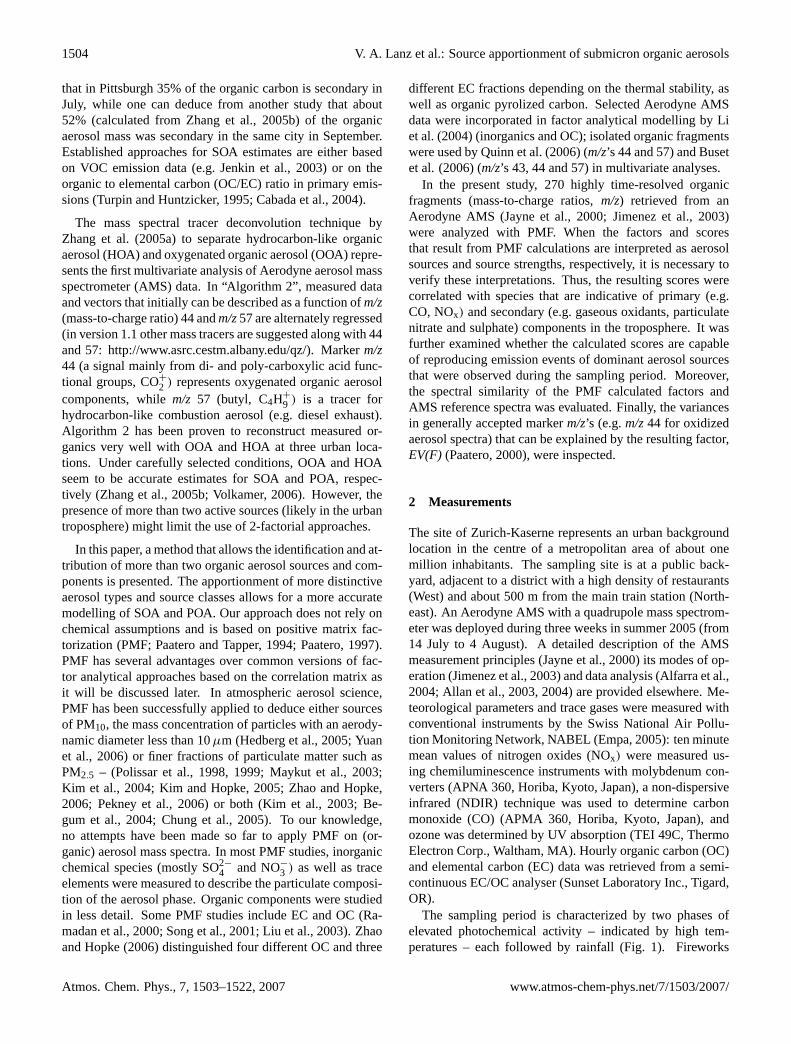
The sampling period is characterized by two phases ofelevated photochemical activity – indicated by high tem-peratures – each followed by rainfall (Fig. 1). Fireworks

Atmos. Chem. Phys., 7, 1503–1522, 2007 www.atmos-chem-phys.net/7/1503/2007/

http://www.asrc.cestm.albany.edu/qz/

V. A. Lanz et al.: Source apportionment of submicron organic aerosols 1505

35

30

25

20

15

15.0

7.20

05

16.0

7.20

05

17.0

7.20

05

18.0

7.20

05

19.0

7.20

05

20.0

7.20

05

21.0

7.20

05

22.0

7.20

05

23.0

7.20

05

24.0

7.20

05

25.0

7.20

05

26.0

7.20

05

27.0

7.20

05

28.0

7.20

05

29.0

7.20

05

30.0

7.20

05

31.0

7.20

05

01.0

8.20

05

02.0

8.20

05

03.0

8.20

05

04.0

8.20

05

4

3

2

1

16.07.2005 21.07.2005 26.07.2005 31.07.2005

25

20

15

10

5

0rain

fall

[mm

min

-1]

tem

pera

ture

[°C

]

AMS-organics [µg m-3

]

Fig. 1. Measured organics (values above 30µg m−3 are not shown), temperature and rainfall during the sampling campaign at Zurich-Kaserne. Aerosol concentrations are given for a CE of unity.

on the Swiss national holiday (night of 1 August) are in-cluded. Nearby log-fires, charbroiling events and deliveryvans caused other isolated peaks of organic aerosol (Fig. 1).

A total number of about 15 000 mass spectra (MS) wereacquired (averaging time = 2 min). These MS are defined byvectors of 300 elements (m/z’s). 270 elements contain reli-able information about the organic aerosol phase (m/z 12–13, 15–20, 24–27, 29–31, 37–38, 41–45, 48–148, 150–181,185, and 187–300). The other m/z’s were excluded due todominant contributions of the air signals (e.g.m/z28, 32 and40 for N2, O2 and Ar, respectively), inorganic species (e.g.m/z 39 and 46 for K and nitrate, respectively), high back-ground levels (e.g.m/z186) or lack of plausible organic frag-ments (e.g.m/z<12). For more details on the interpretationof organic fragments see Allan et al. (2004) and Zhang etal. (2005a).

A collection efficiency (CE) value is required for the esti-mation of aerosol mass concentration measured by the AMS(Alfarra et al., 2004). Due to the lack of collocated PM1measurements, a value of unity was used for the results re-ported in this study. This provides a lower limit estimation ofthe absolute mass concentrations, but does not influence thefindings and the conclusions of this study since major resultsare reported in percentages of total organic mass.

3 Data analysis

Statistical analyses were carried out with the statistical soft-ware R version 2.1.1 (http://www.r-project.org, GNU GEN-ERAL PUBLIC LICENSE Version 2, June 1991) and IGORPRO 5.02 (Wavemetrics Inc., Lake Oswego, OR). Vectors

are represented by bold italic letters, matrices by uppercasebold letters. Single vector and matrix elements as well asequations are written in lowercase italic letters.

3.1 Positive matrix factorization (PMF)

PMF is a well-established program to solve functional mix-ing models and is based on the work of Paatero and Tapper(1994) and Paatero (1997). The associated software “PMF2”(version 4.2) was used in this study. PMF can be used tosolve receptor-only models and is most useful when sourceprofiles are unknown. The fundamental principle of recep-tor modelling is that mass conservation can be assumed anda mass balance analysis can be used to identify and appor-tion sources of airborne particulate matter in the atmosphere(Hopke, 2003). The most important advantages of the PMFprogram compared to common receptor modeling techniquesare that it uses a least-squares algorithm taking data uncer-tainty into account and that its solutions are restricted to thenon-negative subspace. Both features lay the foundation ofmaking the link between the mathematical solution and theprocesses of the real world possible. In practice, sources arebetter separated and positive scores and loadings are physi-cally meaningful (Huang et al., 1999).

PMF is a factor analytical program for bilinear un-mixingof data measured at a receptor site. In PMF, the mass balanceequation

X = GF (1)

is solved, with the measured data matrix,X, that combinesm measurements (in time) ofn variables (m×n matrix). Thep rows of theF matrix (p×n matrix) are called factors (or

www.atmos-chem-phys.net/7/1503/2007/ Atmos. Chem. Phys., 7, 1503–1522, 2007

http://www.r-project.org


loadings), the columns of them×p matrix G are calledscores. The factors can often be interpreted as emissionsource profiles, the corresponding source activity is then rep-resented by the scores. However, the number of sources,p,that have an impact on the data is typically unknown. More-over, for a certain number of factorsp, there is an infinitenumber of mathematically correct solutions to (1) given byrotated matricesG′=G T andF′=T−1 F (where the rotationmatrix, T, multiplied by its inverse,T−1, equals the identitymatrix). Most of these solutions are physically meaninglessdue to negativity. Therefore, PMF imposes non-negativityconstraints to the unmixed matrix elements. In this study,data matrixX consists ofj=1. . .n measured organicm/z’sat i=1. . .m samples in time,ORG. The matrix product ofscores,G, and factors,F, defines the modelled organics,ORG.

X = ORGij =

p∑k=1

Gik Fkj + Eij = ORGij + Eij (2)

wherep is the number of factors (or remaining dimensions ofthe original 270-dimensional space) and matrixE the modelerror. In this equation,Fkj is the modelled profile and andGik the modelled activity of factork. Choosing the rightnumber of factors or dimensions is a critical step in PMF. Of-ten interpretability ofG andF (along with diagnostic PMFvalues) is set as criterion for the optimump. This step re-quires a priori knowledge and is highly subjective. Sec-tion 4.1 will be dedicated to this issue.

Factor matricesG andF form an approximate bilinear de-composition ofORG. This factor analysis problem is solvedby minimizing the error,E, weighted by measurement uncer-tainty matrix,S, (weighted least square solved by a Gauss-Newton algorithm):

Q = arg minG

minF

m∑i=1

n∑j=1

(ORGij − GikFkj

Sij

)2

, (3)

meaning that the value of the argument of the uncertainty(S) weighted difference between the measured (ORG) andmodelled (GF) data matrix is at its minimum with respect toboth fitting factors, the columns ofG as well as the rows ofF.

Thus, accurate uncertainty estimates of measured data areneeded. Error estimates for a given AMS signal in [Hz]

sj = α

√(Ijo + Ijb)

ts(4)

were calculated from the ion signals ofm/z j , Ijo and Ijb

(taking into account that the ion signal at blocked aerosolbeam,Ijb, is subtracted from the open beam signal,Ijo, inorder to calculate the ultimate AMS signal), sampling time,ts , and a statistical distribution factor,α, and then transferredinto organic-equivalent concentrations (org-eq.µg m−3) us-ing the IGOR PRO 5.02 code based on the work of Allan

et al. (2003; http://cloudbase.phy.umist.ac.uk/people/allan/ja igor.htm). PMF was run in the non-robust mode. Other pa-rameters were set to default values and no data pre-treatmentwas performed.

3.2 Interpretation of factors and scores

For interpretation of the factors (rows ofF) calculated byPMF, they were normalized and compared to measured ref-erence spectra (Sects. 3.2.1 and 4.2). The correspondingscores (columns ofG) were correlated with indicative markerspecies of sources and atmospheric processes (Sect. 4.4).Note that both matrices,G andF, have to be estimated fromthe data without assuming any a priori knowledge (with theexception of general non-negativity constraints for the matrixelements). When factors are interpreted as source profiles oraerosol components, they will be labelled with the name ofthe source or aerosol component. The corresponding scoresare then called source activities.

3.2.1 Spectral similarity and reference spectra

The intensities of all obtained loadings (interpreted as massspectra,msj ) with j=1. . . 270m/z’s were first normalized

msnorm.j = msj/

∑j

msj . (5)

The normalized spectra (msnorm.j ) were then correlated with

normalized reference spectra from literature (msref.,norm.j )

and the coefficient of determination (R2) was calculated asa measure of spectral similarity. This gives an objective andsensitive (e.g. theR2 of the mass spectra of diesel and fulvicacid used in this study is 0.03) measure of spectral similarity.Further, it has been applied in similar previous publications(e.g. Zhang et al., 2005a) and is widely applicable and com-monly used. The suitability ofR2 as a measure of spectralsimilarity has been validated by comparing it to other mea-sures of distance, such as an uncertainty-weighted Euclidiandistance, that allowed for the same interpretation. This ap-proach however might have some shortcomings when it isapplied to AMS spectra as such, e.g. the possible leverageeffect of a few, high intensity masses (e.g.m/z18, 29, 43,44) in regression analysis. These masses are typically small(m/z≤44). Therefore, spectral similarity was also calculatedfor m/z>44, R2

m/z>44, providing additional insight into thesimilarity of the low intensity masses only (values in paren-theses; Table 1). The use of both values yields a more robustassessment of similarity.

Reference spectra used for transformed OA include ful-vic acid (a model compound that describes the chemicalfunctionality of aged, oxygenated aerosol; Alfarra, 2004),secondary organic aerosols from VOC precursors such asα-pinene, isoprene, 1,3,5-trimethylbenzene, m-xylene, andcyclopentene (Bahreini et al., 2005; Alfarra et al., 2006a),as well as aged rural and urban aerosol from field studies


http://cloudbase.phy.umist.ac.uk/people/allan/ja_igor.htm

http://cloudbase.phy.umist.ac.uk/people/allan/ja_igor.htm


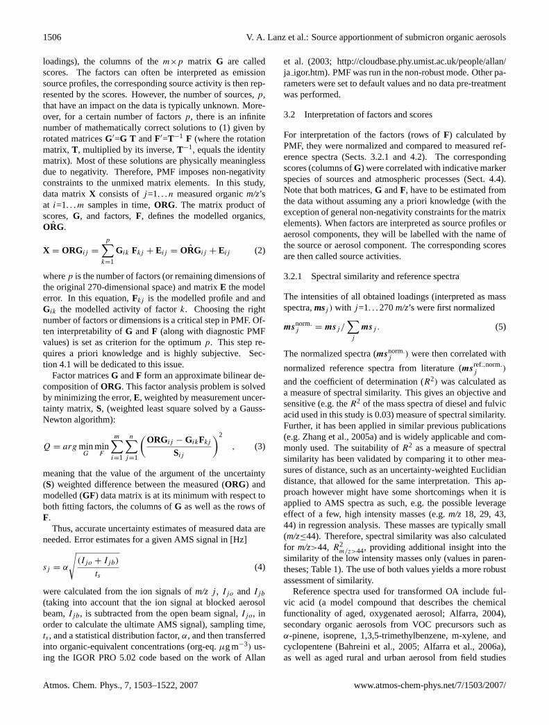
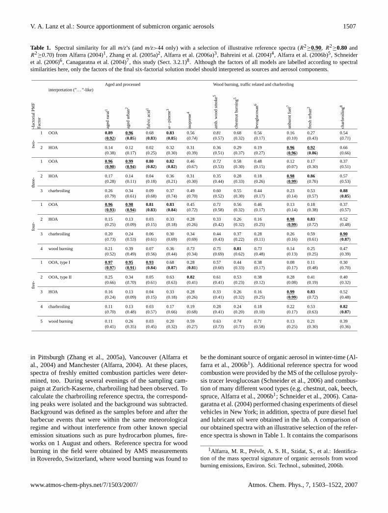
Table 1. Spectral similarity for allm/z’s (and m/z>44 only) with a selection of illustrative reference spectra (R2≥0.90, R2

≥0.80 andR2

≥0.70) from Alfarra (2004)1, Zhang et al. (2005a)2, Alfarra et al. (2006a)3, Bahreini et al. (2004)4, Alfarra et al. (2006b)5, Schneideret al. (2006)6, Canagaratna et al. (2004)7, this study (Sect. 3.2.1)8. Although the factors of all models are labelled according to spectralsimilarities here, only the factors of the final six-factorial solution model should interpreted as sources and aerosol components.

Aged and processed Wood burning, traffic related and charbroiling

-fac

toria

lPM

FF

acto

r

interpretation (”. . . ”-like)

aged

rura

l1

aged

urba

n2

fulv

icac

id1

α−

pine

ne3

isop

rene

4

amb.

woo

dsm

oke5

ches

tnut

burn

ing5

levo

gluc

osan6

unbu

rntf

uel7

fres

hur

ban2

char

broi

ling8

two-

1 OOA 0.89(0.92)

0.96(0.85)

0.68(0.83)

0.83(0.85)

0.56(0.74)

0.81(0.57)

0.68(0.32)

0.56(0.17)

0.16(0.10)

0.27(0.43)

0.54(0.71)

2 HOA 0.14(0.38)

0.12(0.17)

0.02(0.25)

0.32(0.30)

0.31(0.39)

0.36(0.51)

0.29(0.37)

0.19(0.27)

0.96(0.96)

0.92(0.86)

0.66(0.66)

thre

e-

1 OOA 0.96(0.90)

0.99(0.94)

0.80(0.82)

0.82(0.82)

0.46(0.67)

0.72(0.53)

0.58(0.30)

0.48(0.15)

0.12(0.07)

0.17(0.30)

0.37(0.51)

2 HOA 0.17(0.28)

0.14(0.11)

0.04(0.18)

0.36(0.21)

0.31(0.30)

0.35(0.44)

0.28(0.33)

0.18(0.26)

0.98(0.99)

0.86(0.76)

0.57(0.53)

3 charbroiling 0.26(0.79)

0.34(0.61)

0.09(0.68)

0.37(0.74)

0.49(0.70)

0.60(0.52)

0.55(0.30)

0.44(0.17)

0.23(0.14)

0.53(0.57)

0.88(0.85)

four

-

1 OOA 0.96(0.93)

0.98(0.94)

0.81(0.83)

0.83(0.84)

0.45(0.72)

0.71(0.58)

0.56(0.32)

0.46(0.17)

0.13(0.14)

0.18(0.38)

0.37(0.57)

2 HOA 0.15(0.25)

0.13(0.09)

0.03(0.15)

0.33(0.18)

0.28(0.26)

0.33(0.42)

0.26(0.32)

0.16(0.25)

0.98(0.99)

0.83(0.72)

0.52(0.48)


0.24(0.53)

0.06(0.61)

0.30(0.69)

0.34(0.69)

0.44(0.43)

0.37(0.22)

0.28(0.11)

0.26(0.16)

0.59(0.61)

0.90(0.87)

4 wood burning 0.21(0.52)

0.39(0.49)

0.07(0.56)

0.36(0.44)

0.73(0.34)

0.75(0.69)

0.81(0.62)

0.73(0.48)

0.14(0.13)

0.25(0.25)

0.47(0.39)

five-

1 OOA, type I 0.97(0.97)

0.95(0.91)

0.93(0.84)

0.68(0.87)

0.28(0.81)

0.57(0.60)

0.44(0.33)

0.38(0.17)

0.08(0.17)

0.11(0.48)

0.30(0.70)

2 OOA, type II 0.25(0.66)

0.34(0.70)

0.05(0.61)

0.63(0.63)

0.82(0.41)

0.61(0.41)

0.53(0.23)

0.38(0.12)

0.28(0.08)

0.41(0.19)

0.40(0.32)

3 HOA 0.16(0.24)

0.13(0.09)

0.04(0.15)

0.33(0.18)

0.28(0.26)

0.33(0.41)

0.26(0.32)

0.16(0.25)

0.99(0.99)

0.83(0.72)

0.52(0.48)


0.13(0.48)

0.03(0.57)

0.17(0.66)

0.19(0.68)

0.28(0.41)

0.24(0.20)

0.18(0.10)

0.22(0.17)

0.53(0.63)

0.82(0.87)


0.26(0.35)

0.03(0.45)

0.20(0.32)

0.59(0.27)

0.63(0.73)

0.74(0.71)

0.71(0.58)

0.13(0.25)

0.21(0.30)

0.39(0.36)

in Pittsburgh (Zhang et al., 2005a), Vancouver (Alfarra etal., 2004) and Manchester (Alfarra, 2004). At these places,spectra of freshly emitted combustion particles were deter-mined, too. During several evenings of the sampling cam-paign at Zurich-Kaserne, charbroiling had been observed. Tocalculate the charbroiling reference spectra, the correspond-ing peaks were isolated and the background was subtracted.Background was defined as the samples before and after thebarbecue events that were within the same meteorologicalregime and without interference from other known specialemission situations such as pure hydrocarbon plumes, fire-works on 1 August and others. Reference spectra for woodburning in the field were obtained by AMS measurementsin Roveredo, Switzerland, where wood burning was found to

be the dominant source of organic aerosol in winter-time (Al-farra et al., 2006b1). Additional reference spectra for woodcombustion were provided by the MS of the cellulose pyroly-sis tracer levoglucosan (Schneider et al., 2006) and combus-tion of many different wood types (e.g. chestnut, oak, beech,spruce, Alfarra et al., 2006b1; Schneider et al., 2006). Cana-garatna et al. (2004) performed chasing experiments of dieselvehicles in New York; in addition, spectra of pure diesel fueland lubricant oil were obtained in the lab. A comparison ofour obtained spectra with an illustrative selection of the refer-ence spectra is shown in Table 1. It contains the comparisons

1Alfarra, M. R., Prevot, A. S. H., Szidat, S., et al.: Identifica-tion of the mass spectral signature of organic aerosols from woodburning emissions, Environ. Sci. Technol., submitted, 2006b.



Table 1. Continued.

Aged and processed Wood burning, traffic related and charbroiling

-fac

toria

lPM

FF

acto

r

interpretation (”. . . ”-like)

aged

rura

l1

aged

urba

n2

fulv

icac

id1

α−

pine

ne3

isop

rene

4

amb.

woo

dsm

oke5

ches

tnut

burn

ing5

levo

gluc

osan6

unbu

rntf

uel7

fres

hur

ban2

char

broi

ling8

six-

1 OOA, type I 0.96(0.96)

0.93(0.93)

0.96(0.83)

0.63(0.84)

0.23(0.79)

0.52(0.62)

0.40(0.35)

0.35(0.19)

0.06(0.18)

0.08(0.45)

0.25(0.65)

2 OOA, type II 0.27(0.86)

0.34(0.79)

0.05(0.75)

0.65(0.83)

0.80(0.65)

0.62(0.51)

0.53(0.27)

0.37(0.13)

0.33(0.16)

0.50(0.42)

0.49(0.61)

3 HOA 0.15(0.23)

0.12(0.08)

0.03(0.14)

0.32(0.16)

0.27(0.25)

0.31(0.40)

0.25(0.32)

0.15(0.25)

0.99(0.99)

0.81(0.70)

0.50(0.46)


0.19(0.49)

0.06(0.57)

0.23(0.67)

0.22(0.68)

0.33(0.40)

0.28(0.19)

0.20(0.09)

0.23(0.16)

0.54(0.61)

0.85(0.86)


0.46(0.35)

0.17(0.45)

0.28(0.29)

0.56(0.28)

0.73(0.74)

0.82(0.74)

0.82(0.63)

0.09(0.23)

0.15(0.27)

0.38(0.34)

6 minor/cooking 0.24(0.62)

0.33(0.48)

0.05(0.53)

0.50(0.57)

0.70(0.45)

0.67(0.54)

0.63(0.36)

0.46(0.22)

0.35(0.28)

0.53(0.47)

0.64(0.58)

seve

n-

1 OOA, type I 0.94(0.95)

0.90(0.92)

0.97(0.82)

0.60(0.83)

0.20(0.79)

0.48(0.61)

0.37(0.34)

0.32(0.18)

0.05(0.19)

0.07(0.46)

0.23(0.65)

2 OOA, type II 0.26(0.86)

0.33(0.79)

0.05(0.74)

0.65(0.83)

0.79(0.64)

0.60(0.50)

0.51(0.26)

0.35(0.12)

0.33(0.15)

0.49(0.40)

0.47(0.59)


0.20(0.50)

0.06(0.57)

0.24(0.67)

0.23(0.68)

0.34(0.40)

0.28(0.19)

0.21(0.09)

0.24(0.15)

0.55(0.61)

0.86(0.86)

4 HOA 0.14(0.24)

0.11(0.09)

0.03(0.15)

0.31(0.17)

0.27(0.26)

0.31(0.41)

0.24(0.32)

0.15(0.25)

0.99(0.99)

0.82(0.72)

0.51(0.47)


0.65(0.42)

0.36(0.46)

0.37(0.32)

0.54(0.35)

0.77(0.84)

0.82(0.83)

0.83(0.71)

0.08(0.31)

0.12(0.36)

0.37(0.44)

6 minor/unknown 0.34(0.46)

0.44(0.37)

0.15(0.49)

0.46(0.43)

0.56(0.35)

0.70(0.49)

0.69(0.38)

0.55(0.26)

0.25(0.18)

0.40(0.32)

0.63(0.42)

7 minor/cooking 0.29(0.61)

0.38(0.47)

0.08(0.50)

0.52(0.55)

0.70(0.46)

0.71(0.54)

0.67(0.35)

0.51(0.22)

0.35(0.29)

0.53(0.49)

0.67(0.59)

of all factors deduced from 2- to 7-factorial PMF (n=27) withthe selected reference spectra (n=11). This comparison isbased on spectral similaritiesR2 andR2

m/z>44 (in brackets)as defined before. The most interesting results of this 594element table will be discussed in detail later in Sect. 4.2.

4 Results and discussion

4.1 Determination of the number of factors

In PMF, choosing the number of factors often needs a com-promise. Using too few factors will coerce sources of differ-ent types into one factor, while using too many will split realsources into unreal factors. PMF is a descriptive model andthere is no objective criterion to choose the ideal solution.

“Interpretability” (or “meaningfulness”) is frequently usedto determine the number of factors (e.g. Li et al., 2004; Busetet al., 2006). Mathematical PMF diagnostics (model error,Q, rotational ambiguity,rotmat , etc.) characterize technical

aspects of the solution. However, they do not guarantee thebest solution in terms of explaining real-world phenomena.Rigorous testing of the plausibility of PMF solutions (thatare basically blind to atmospheric processes) should be basedon accompanying measurements of trace gases, aerosols andmeteorology (Sects. 4.2, 4.4 and 4.5).

4.1.1 Mathematical diagnostics

For the 6-factorial solution, only a small fraction (<1%) ofthe scaled residuals,E(scaled)or (X-GF)/S, exceeds the de-fault outlier limits of−4 and 4 (the most explanatory poweris given for the 6-factorial solution as discussed in Sect. 4.2).The total sum of squared scaled residuals (Eq. 3),Q, relativeto its expected value,Q.exp, that can be approximated by thenumber of data matrix elements, does not exceed a value ofabout two for models with more than two factors. The ra-tio Q/Q.expis about one for six and more factors (Fig. 2a),meaning that error estimates based on Eq. (4) are accurate



5.740

5.739

5.738

5.737

5.736

5.735

x106

-0.6 -0.4 -0.2 0.0 0.2 0.4 0.6fpeak

0.3

0.2

0.1

0.0

12108642

� � �(fpeak) log(��)

0.9992

0.9988

0.9984

0.9980

12108642

6

4

2

0

x10-3

R2

��

5

4

3

2

1

0

28024020016012080400 m/z

25

20

15

10

5

0

54321

1284

x103

� contribution per �� contribution per sample photochemical phase non-photochemical phaseSNR (m/z 43)

SNR (m/z 29)

row/sample [103]

SNR

a. �-values

c. model fit (R2), rotational ambiguity (�� )

b. � contributions and signal-to-noise ratios (SNR)

number of factors

number of factors

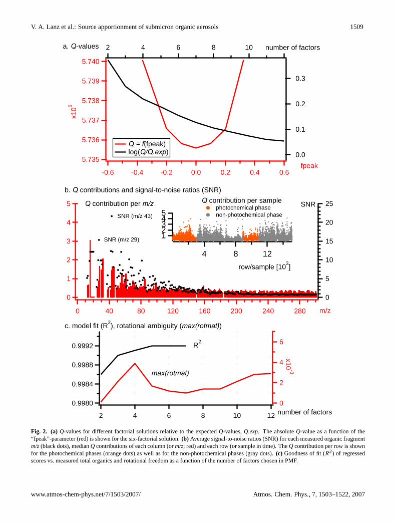
Fig. 2. (a) Q-values for different factorial solutions relative to the expectedQ-values,Q.exp. The absoluteQ-value as a function of the“fpeak”-parameter (red) is shown for the six-factorial solution.(b) Average signal-to-noise ratios (SNR) for each measured organic fragmentm/z(black dots), medianQ contributions of each column (orm/z; red) and each row (or sample in time). TheQ contribution per row is shownfor the photochemical phases (orange dots) as well as for the non-photochemical phases (gray dots).(c) Goodness of fit (R2) of regressedscores vs. measured total organics and rotational freedom as a function of the number of factors chosen in PMF.



0.15

0.10

0.05

0.0016014012010080604020

b. OOA, type II [norm. int.]

43

15 29

55

0.10

0.05

0.0016014012010080604020

c. charbroiling [norm. int.]2741 55

6781 91

95

60

40

20

0

16014012010080604020m/z

201510

5

280240200

264

158

4315 29

55115

69

e. minor source [10-3

norm. int.]

91

80604020

016014012010080604020

6073

29

15

11591

44

d. wood burning [10-3

norm. int.]

0.15

0.10

0.05

0.0016014012010080604020

c. HOA [norm. int.]

43

718529

57

5541

6927 83

0.16

0.12

0.08

0.04

0.0016014012010080604020

a. OOA, type I [norm. int.]

18 44

29

55

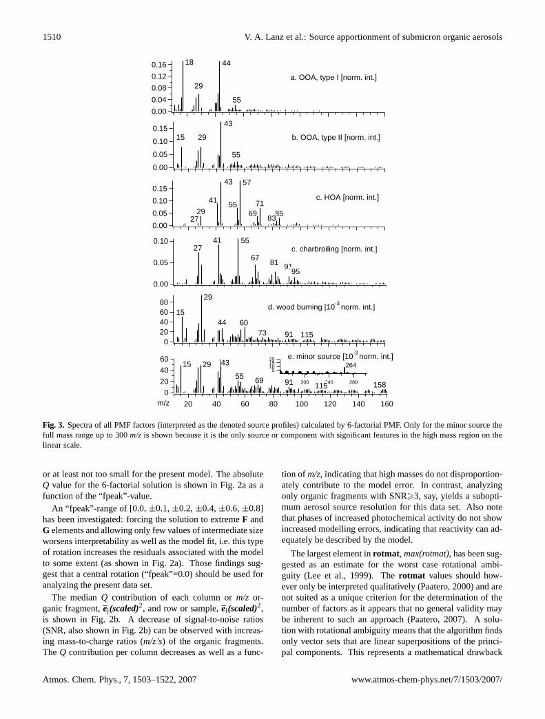
Fig. 3. Spectra of all PMF factors (interpreted as the denoted source profiles) calculated by 6-factorial PMF. Only for the minor source thefull mass range up to 300m/z is shown because it is the only source or component with significant features in the high mass region on thelinear scale.

or at least not too small for the present model. The absoluteQ value for the 6-factorial solution is shown in Fig. 2a as afunction of the “fpeak”-value.

An “fpeak”-range of [0.0,±0.1,±0.2,±0.4,±0.6,±0.8]has been investigated: forcing the solution to extremeF andG elements and allowing only few values of intermediate sizeworsens interpretability as well as the model fit, i.e. this typeof rotation increases the residuals associated with the modelto some extent (as shown in Fig. 2a). Those findings sug-gest that a central rotation (“fpeak”=0.0) should be used foranalyzing the present data set.

The medianQ contribution of each column orm/z or-ganic fragment,ej(scaled)2, and row or sample,ei(scaled)2,is shown in Fig. 2b. A decrease of signal-to-noise ratios(SNR, also shown in Fig. 2b) can be observed with increas-ing mass-to-charge ratios (m/z’s) of the organic fragments.TheQ contribution per column decreases as well as a func-

tion of m/z, indicating that high masses do not disproportion-ately contribute to the model error. In contrast, analyzingonly organic fragments with SNR>3, say, yields a subopti-mum aerosol source resolution for this data set. Also notethat phases of increased photochemical activity do not showincreased modelling errors, indicating that reactivity can ad-equately be described by the model.

The largest element inrotmat , max(rotmat), has been sug-gested as an estimate for the worst case rotational ambi-guity (Lee et al., 1999). Therotmat values should how-ever only be interpreted qualitatively (Paatero, 2000) and arenot suited as a unique criterion for the determination of thenumber of factors as it appears that no general validity maybe inherent to such an approach (Paatero, 2007). A solu-tion with rotational ambiguity means that the algorithm findsonly vector sets that are linear superpositions of the princi-pal components. This represents a mathematical drawback



as the solution is not unique, i.e. the resolved factors canbe rotated without changing the residuals associated withthe model (rotational ambiguity hampers the qualitative in-terpretation of the results). There are three local minima inmax(rotmat)versus number of factors shown in Fig. 2c: oneat two factors (max(rotmat)=0.0001) and one at seven factors(max(rotmat)=0.0010). Values similar to the second mini-mum can be found from five to nine factors, supporting theactual choice ofp=6 factors based on interpretability. The 2-factorial solution with lowest rotational ambiguity exhibitssuboptimum aerosol source resolution as discussed below(e.g. see Sect. 4.3). The third local minimum is at 15 factors(max(rotmat)=0.0026), but uninterpretable factors (e.g. over-whelming dominance ofm/z15 or m/z41) can be observedas soon as the number of sources is increased from sevento eight (in Sect. 4.2 we describe what happens, when thenumber of factors is gradually increased from two to sevensources).

In addition, the fit of the regressed scores to measured or-ganics for all PMF solutions was investigated,

orgi = a +

p∑k=1

bkgik, (6)

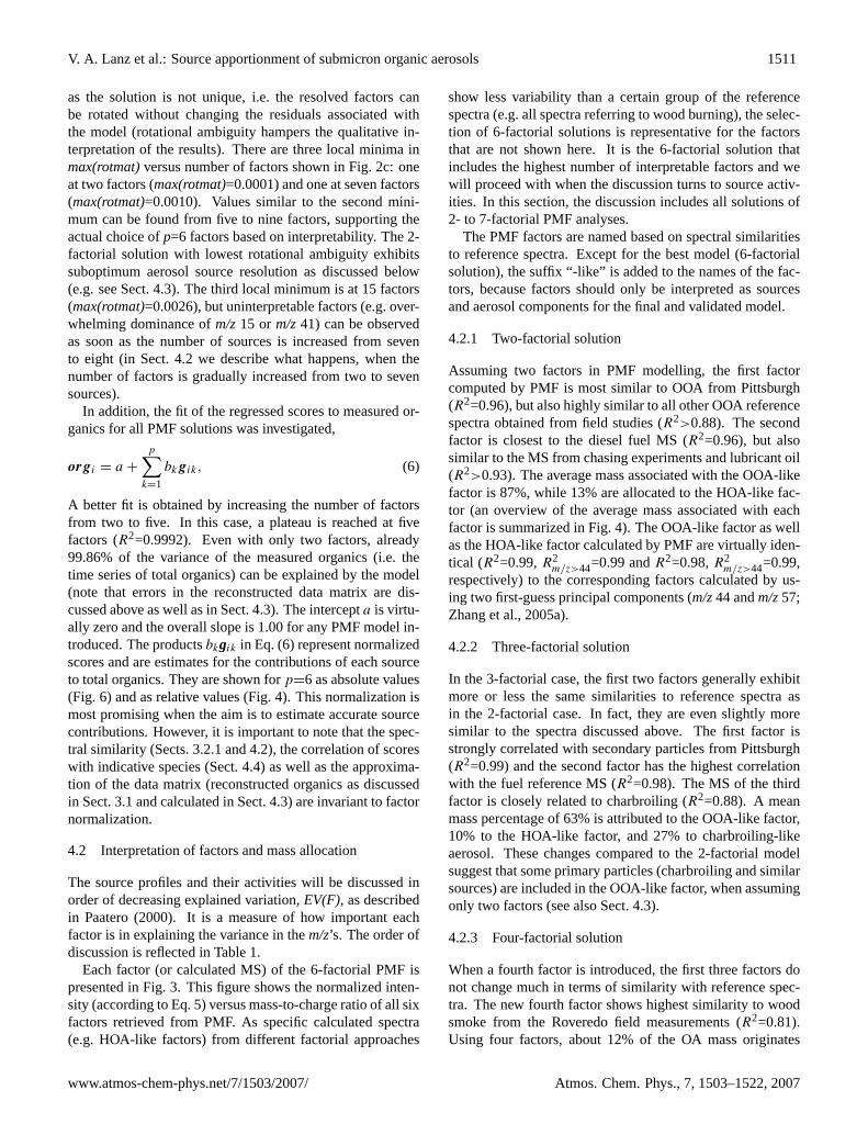
A better fit is obtained by increasing the number of factorsfrom two to five. In this case, a plateau is reached at fivefactors (R2=0.9992). Even with only two factors, already99.86% of the variance of the measured organics (i.e. thetime series of total organics) can be explained by the model(note that errors in the reconstructed data matrix are dis-cussed above as well as in Sect. 4.3). The intercepta is virtu-ally zero and the overall slope is 1.00 for any PMF model in-troduced. The productsbkgik in Eq. (6) represent normalizedscores and are estimates for the contributions of each sourceto total organics. They are shown forp=6 as absolute values(Fig. 6) and as relative values (Fig. 4). This normalization ismost promising when the aim is to estimate accurate sourcecontributions. However, it is important to note that the spec-tral similarity (Sects. 3.2.1 and 4.2), the correlation of scoreswith indicative species (Sect. 4.4) as well as the approxima-tion of the data matrix (reconstructed organics as discussedin Sect. 3.1 and calculated in Sect. 4.3) are invariant to factornormalization.

4.2 Interpretation of factors and mass allocation

The source profiles and their activities will be discussed inorder of decreasing explained variation,EV(F), as describedin Paatero (2000). It is a measure of how important eachfactor is in explaining the variance in them/z’s. The order ofdiscussion is reflected in Table 1.

Each factor (or calculated MS) of the 6-factorial PMF ispresented in Fig. 3. This figure shows the normalized inten-sity (according to Eq. 5) versus mass-to-charge ratio of all sixfactors retrieved from PMF. As specific calculated spectra(e.g. HOA-like factors) from different factorial approaches

show less variability than a certain group of the referencespectra (e.g. all spectra referring to wood burning), the selec-tion of 6-factorial solutions is representative for the factorsthat are not shown here. It is the 6-factorial solution thatincludes the highest number of interpretable factors and wewill proceed with when the discussion turns to source activ-ities. In this section, the discussion includes all solutions of2- to 7-factorial PMF analyses.

The PMF factors are named based on spectral similaritiesto reference spectra. Except for the best model (6-factorialsolution), the suffix “-like” is added to the names of the fac-tors, because factors should only be interpreted as sourcesand aerosol components for the final and validated model.

4.2.1 Two-factorial solution

Assuming two factors in PMF modelling, the first factorcomputed by PMF is most similar to OOA from Pittsburgh(R2=0.96), but also highly similar to all other OOA referencespectra obtained from field studies (R2>0.88). The secondfactor is closest to the diesel fuel MS (R2=0.96), but alsosimilar to the MS from chasing experiments and lubricant oil(R2>0.93). The average mass associated with the OOA-likefactor is 87%, while 13% are allocated to the HOA-like fac-tor (an overview of the average mass associated with eachfactor is summarized in Fig. 4). The OOA-like factor as wellas the HOA-like factor calculated by PMF are virtually iden-tical (R2=0.99,R2

m/z>44=0.99 andR2=0.98,R2m/z>44=0.99,

respectively) to the corresponding factors calculated by us-ing two first-guess principal components (m/z44 andm/z57;Zhang et al., 2005a).

4.2.2 Three-factorial solution

In the 3-factorial case, the first two factors generally exhibitmore or less the same similarities to reference spectra asin the 2-factorial case. In fact, they are even slightly moresimilar to the spectra discussed above. The first factor isstrongly correlated with secondary particles from Pittsburgh(R2=0.99) and the second factor has the highest correlationwith the fuel reference MS (R2=0.98). The MS of the thirdfactor is closely related to charbroiling (R2=0.88). A meanmass percentage of 63% is attributed to the OOA-like factor,10% to the HOA-like factor, and 27% to charbroiling-likeaerosol. These changes compared to the 2-factorial modelsuggest that some primary particles (charbroiling and similarsources) are included in the OOA-like factor, when assumingonly two factors (see also Sect. 4.3).

4.2.3 Four-factorial solution

When a fourth factor is introduced, the first three factors donot change much in terms of similarity with reference spec-tra. The new fourth factor shows highest similarity to woodsmoke from the Roveredo field measurements (R2=0.81).Using four factors, about 12% of the OA mass originates



100

90

80

70

60

50

40

30

20

10

0aver

age

mas

s co

ntrib

utio

n to

tota

l org

anic

s [%

]

1312111098765432 number of factors

2 3 4 5 6 7

aerosol sources/components:

HOA(-like) wood burning(-like) charbroiling(-like) minor source (cooking) minor source OOA(-like) OOA, type I OOA, type II

40%44%

19%

11%

22%22%

12%8%

6%

10%

7%10%

27%

60%

10%

10%

7%7%

7%

62%

13%

87%

6%

20%

50%

15%

6%

Fig. 4. Average mass allocation to each PMF-solution assuming two to seven factors.

from wood burning-like aerosol. When the wood burning-like factor is introduced, modelled mass from charbroiling-like aerosol is reduced most (difference between the massattributed within the 3-factorial approach and the one withinthe 4 factorial approach:1mass=−7%).

4.2.4 Five-factorial solution

A dramatic change can be observed when five factors areused in PMF modelling: not as much in the change ofmax(rotmat)or the model fit (Sect. 4.1), but in terms of simi-larity to secondary aerosol. The original first, OOA-like fac-tor is split into highly aged background aerosol (high sim-ilarity to aged rural aerosol:R2=0.97 and to fulvic acid:R2=0.93) and one that mostly resembles aerosol from iso-prene oxidation in the presence of NOx (R2=0.82). We willrefer to these OOA factors as “OOA, type I” and “OOA,type II”, respectively. The third spectrum is again associ-ated with charbroiling (R2=0.82), the fourth with wood burn-ing (similarity to Roveredo spectra:R2=0.70; levoglucosan:R2=0.71). Increasing the number of factors from four tofive does not affect the modelled mass of wood burning-likeaerosol (1mass=−2%) or fuel-like aerosol (1mass=−1%),while charbroiling-like aerosol again (1mass=−6%) is losingmost of its contribution. This indicates that using only threeor four factors results in overestimating OA from charbroil-ing.

4.2.5 Six-factorial solution

With six factors, the first factor is even more similar to ful-vic acid (R2=0.96), while the third factor is still very similarto fuel aerosol (R2=0.99). The second factor can be inter-preted similarly as in the 5-factorial case. However, consid-ering only m/z>44, correlations are highest withα-pineneSOA rather than isoprene SOA. It should be noted that in re-ality SOA from several precursors will contribute to this fac-

tor, where the differences between the reference spectra donot seem to be significant enough to discriminate betweenthose. The fourth factor can be interpreted as a charbroilingsource again (R2=0.85), the fifth is even more levoglucosan-like (R2=0.82). The sixth factor does not fit in any class ofreference spectra, but there is an indication for a fragmen-tation that resembles an oleic acid type signature that mayarise from food cooking: the mass spectrum of this factoris characterised bym/z264 with an intensity of about 15%relative to the largest peak (m/z 43) and it is in the samerange asm/z60 in this factor. This might be an indicationof oleic acid (NIST, 2006), the most abundant monoenoicfatty acid in plant and animal tissues. On the other hand,Katrib et al. (2004) showed thatm/z264 is much more de-pleted in pure oleic acid than shown in this factor. There-fore, this is an indication that oleic acid might be lumpedtogether with other similar fatty acids, such as petroselenicacid (which is present e.g. in coriander and parsley), pointingto food cooking as a partial source in that factor (additionalevidence that this factor might include food cooking aerosolswill be given in Sect. 4.4.3). However, a conclusive compar-ison should be based on measured reference spectra for foodcooking aerosol rather than on the mass spectrum of modelsubstances (such as oleic acid). To our knowledge, no suchspectra can be found in the published AMS literature. Goingfrom five to six factors, the average mass does not change forfuel-like aerosols. In general, mass differences for all factorsare small (|1mass| ≤5%).

4.2.6 Seven-factorial solution

The first five factors in the 7-factorial solution are more orless the same as with six factors. The seventh factor, ten-tatively assigned to food cooking, remains unchanged too,while the sixth factor does not correlate well with any ofthe available reference spectra: similarity is highest with thewood burning MS but correlations are lower than for the



fifth factor. If the sixth factor is added to the fifth factor(interpreted as wood burning), the resulting factor exhibitsincreased correlation (R2=0.84, R2

m/z>44=0.87) to ambientwood burning aerosols from Roveredo (but the same or lowercorrelation to other measured wood smoke spectra). This in-dicates that splitting real sources into unreal factors by as-suming too many factors might already start at 7-factorialsolutions to some extent. In addition, no more significantchanges in the mass contribution to total organics take place,when we assume seven instead of six factors: charbroiling-like (10%) and traffic-related fuel aerosol (6%) aerosol re-main at constant levels, the minor source that might be in-fluenced by food cooking (1mass=−1%) and aerosol that re-sembles OOA from local precursors (1mass=+1%) are almostunchanged.

4.2.7 Evaluation of 2- to 7-factorial solutions

In summary, choosing only two factors in factor analyti-cal models for this site overestimates OOA if interpretedas SOA. At sites with two dominating sources this may beless critical; as an example, Zhang et al. (2006)2 show thatthis OOA overestimation does not apply for the Pittsburghdataset.

When three and more factors are assumed, aerosol fromprimary sources is subtracted from the OOA-like factor andthis first factor exhibits higher correlations with the massspectrum of fulvic acid.

The similarity of this first factor to fulvic acid is mainlyincreased when the number of factors is changed from twoto three as well as from four to five. About 85–90% percentof the overallm/z44 variance can be explained by this firstfactor. Evidence form/z44 andm/z57 as tracers for oxy-genated and hydrocarbon aerosol was first given in Alfarra etal. (2004).

A HOA-like factor is salient from 2- to 7-factorial PMF.The fraction of OA explained by the HOA-like factor is de-creasing from 13% in the 2-factorial approach to 6–7% in the4- to 7-factorial approaches. The similarity to fuel is alreadystrong when using only two factors. Strongest similarity isreached when five factors are used. Most of the variancein the diesel markerm/z57 can be explained by the HOA-like factor. In the 2-factorial case, this amounts to 80% andmonotonously decreases with each additional source down toabout 50%. The wood burning-like factor explains 12–13%of them/z57 variance.

When only three factors are chosen, wood burning-likeaerosol is mainly lumped together with charbroiling-likeaerosol (Sect. 4.2.3). Adding a fourth factor takes accountof the fact that there is wood burning in summer (log-fires,

2Zhang, Q., Jimenez, J.-L., Dzepina, K., et al.: Component anal-ysis of organic aerosols in urban, rural, and remote site atmospheresbased on aerosol mass spectrometry, 7th International Aerosol Con-ference, poster 5H8, St. Paul, Minnesota, USA, 2006.

barbecues, as well as domestic garden and forest wood burn-ing). At least four factors are necessary to identify woodburning. The factor identified as wood burning explains 45–55% of all variance inm/z60. About 25% ofm/z60 cannotbe explained by the PMF models. About 25% of them/z73variance is explained by the charbroiling factor and nearly20% by the wood burning factor, while 23% remain unex-plained. Mass-to-charge ratio 60 and 73, as well as 137 havebeen linked to wood burning by Schneider et al. (2006) aswell as by Alfarra et al. (2006b)1. The wood burning-likefactor can account for 30–45% of them/z137 variance, andabout 30% can not be explained by the model.

When a fifth factor is assumed, OOA is divided into highlyaged background aerosol, which is fulvic acid-like and a sec-ond type that can not be clearly assigned to any reference MS(considering both,R2 andR2

m/z>44, see Table 1). Choosingfive, six or seven factors does not affect the solution signif-icantly. Choosing more than seven factors generates sourceprofiles that cannot be interpreted. Changes from six to sevenfactors are very small. Additionally, the average mass as-sociated with each source does not change much when weincrease the number of factors from five to six factors, andeven less when choosing seven instead of six factors (Fig. 4).With five factors, the similarity plateau (defined byR2 of7-factorial solutions, which typically exhibit the highest val-ues) is not attained in most cases (Table 1), whereas the sim-ilarity to isoprene is highest with five factors. Therefore(and because of the findings from the 7-factorial solution,Sect. 4.2.6), using 6 factors might be a good compromise forfurther analyses. The spectra of these six factors are shownin Fig. 3.

4.3 Primary sources contributing to OOA (calculated by 2-factorial PMF)

In Sect. 4.2.2, it was hypothesized that the first factor of2-factorial PMF (interpreted as OOA) includes oxidizedspecies from primary sources. Further evidence that 2-factorial PMF overestimates secondary aerosol at this site,if the factor interpreted as OOA is equated with SOA isgiven here. We would expect that periods of anticyclonic,stable weather conditions, when oxidized aerosol speciesfrom primary sources (e.g. charbroiling, wood burning, to-bacco smoke, food cooking) interfere with oxidized sec-ondary aerosols, are most erroneously modelled by usingtwo-factors only. In such situations, the 2-factorial model isexpected to be less accurate than for instance the 3-factorialapproach.

With respect to the time series of total organics, all usedPMF approaches (2- to 7-factorial) can technically model thedata almost perfectly (Sect. 4.1.1). However, the regressionas given in Eq. (6) does not cover all matrix errors. There-fore, the error patterns in those models should be investi-gated by considering the sum of the absolute model residuals(or absolute differences between the measured data matrix,



1.0

0.8

0.6

0.4

0.2

17.07.2005 21.07.2005 25.07.2005 29.07.2005 02.08.2005Date and Time

1.0

0.8

0.6

0.4

0.2

ei (rel.) 2-factorial PMF ei (rel.) 3-factorial PMF

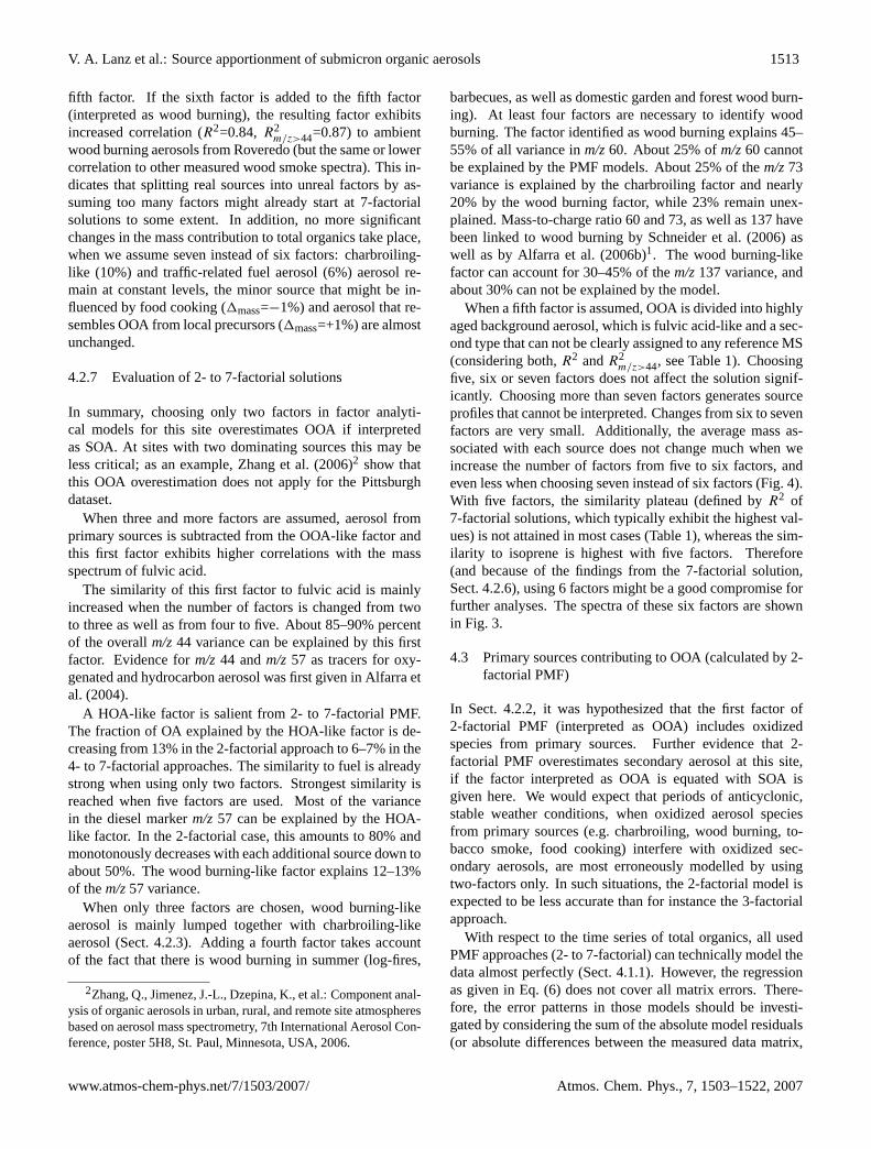
Fig. 5. Different error patterns in 2- and 3-factorial PMF. (The general error patterns of the 4- to 7-factorial solutions can be represented bythe error pattern of the 3-factorial solution.)

ORG, and its model approximate,ORG) divided by the sumof the measured organics.

ei(rel.) =

∑j

∣∣∣ORGij − ORGij

∣∣∣∑j

ORGij

(7)

Periods of elevated photochemistry (as well as 1 August)are indeed more erroneously modelled by 2-factorial PMF(Fig. 5) compared to the 3-factor solution. In contrast, theerrors,ei (rel.), are more or less identical during periods oflow photochemistry (19–25 July and 30 July–4 August; withthe exception of the morning of 1 August). Note that for thesquared scaled residuals (ei(scaled)2) of the 6-factorial solu-tion, those periods exhibit a similar error pattern (Fig. 2b).

4.4 Interpretation of scores (activity of sources)

4.4.1 Processed and volatile OOA

Particulate AMS-sulphate is correlated with OOA, type I(R2=0.52, n=14914). Both time series are shown in Fig. 6and all discussed correlations are presented in Table 2. At-mospheric oxidants (O3+NO2) are also correlated to OOA,type I (R2=0.51), giving further evidence that OOA, type Irefers to highly aged and processed organic aerosol. ThisOOA type is relatively stable during the photochemical pe-riod and exhibits a slight maximum in the afternoon, whentemperature is highest. This suggests that the aerosol mod-elled by OOA, type I is thermodynamically stable. This is,together with the spectral similarity to fulvic acid, stronglyindicating that OOA, type I represents aged, processed andpossibly oligomerized OOA with low volatility as found inSOA from smog chamber studies (Kalberer et al., 2004).

In contrast, OOA, type II shows diurnal patterns withmaxima typically found at night. During the photochemi-cal phase, the baseline of OOA, type II is clearly elevated(Fig. 6). Both findings indicate a general accumulation ofoxidation products formed during the day that condense ontopre-existing particles at night. This latter process is reflectedby OOA, type II. Particle-nitrate retrieved from AMS mea-surements shows a high correlation (R2=0.55) with OOA,type II when the last fifth of the sampling period is excluded(see below). The particulate nitrate concentration dependsstrongly on temperature, as the formation of condensed phaseammonium nitrate is in a temperature and humidity depen-dent equilibrium with ammonia and nitric acid in the gasphase. These findings suggest that OOA, type II is a volatilefraction of OOA with high anti-correlation to the tempera-ture (e.g. if we consider the first four days of the campaign– those are all associated with elevated photochemistry –a relationship of OOA, type II=−0.13·temperature + 5.09,R2=0.47, can be described). In fact, this volatile fraction ofOOA is even more strongly dependent on temperature whenits measurement series is shifted back in time about half aday (R2=0.66). This might suggest that concentrations arehighest in the night after a day with high photochemical ac-tivity when more condensable organics are available. As of 1August (the Swiss National day), the concentrations of mea-sured nitrate and modelled OOA, type II diverge. These lastdays of the campaign are characterized by lower tempera-tures (T<23◦C). This suggests that during this period pho-tochemical oxidation of SOA precursors is low while theformation of nitrate is still high, possibly due to night-timechemistry. Also influences from fireworks on measured ni-trate concentrations cannot be excluded.



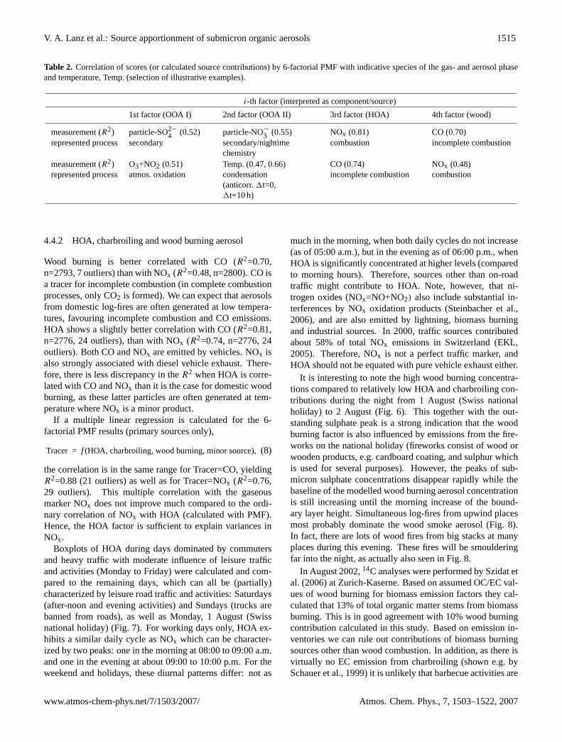
Table 2. Correlation of scores (or calculated source contributions) by 6-factorial PMF with indicative species of the gas- and aerosol phaseand temperature, Temp. (selection of illustrative examples).

i-th factor (interpreted as component/source)

1st factor (OOA I) 2nd factor (OOA II) 3rd factor (HOA) 4th factor (wood)

measurement (R2) particle-SO2−

4 (0.52) particle-NO−3 (0.55) NOx (0.81) CO (0.70)represented process secondary secondary/nightime

chemistrycombustion incomplete combustion

measurement (R2) O3+NO2 (0.51) Temp. (0.47, 0.66) CO (0.74) NOx (0.48)represented process atmos. oxidation condensation

(anticorr.1t=0,1t=10 h)

incomplete combustion combustion

4.4.2 HOA, charbroiling and wood burning aerosol

Wood burning is better correlated with CO (R2=0.70,n=2793, 7 outliers) than with NOx (R2=0.48, n=2800). CO isa tracer for incomplete combustion (in complete combustionprocesses, only CO2 is formed). We can expect that aerosolsfrom domestic log-fires are often generated at low tempera-tures, favouring incomplete combustion and CO emissions.HOA shows a slightly better correlation with CO (R2=0.81,n=2776, 24 outliers), than with NOx (R2=0.74, n=2776, 24outliers). Both CO and NOx are emitted by vehicles. NOx isalso strongly associated with diesel vehicle exhaust. There-fore, there is less discrepancy in theR2 when HOA is corre-lated with CO and NOx than it is the case for domestic woodburning, as these latter particles are often generated at tem-perature where NOx is a minor product.

If a multiple linear regression is calculated for the 6-factorial PMF results (primary sources only),

Tracer = f (HOA, charbroiling, wood burning, minor source),(8)

the correlation is in the same range for Tracer=CO, yieldingR2=0.88 (21 outliers) as well as for Tracer=NOx (R2=0.76,29 outliers). This multiple correlation with the gaseousmarker NOx does not improve much compared to the ordi-nary correlation of NOx with HOA (calculated with PMF).Hence, the HOA factor is sufficient to explain variances inNOx.

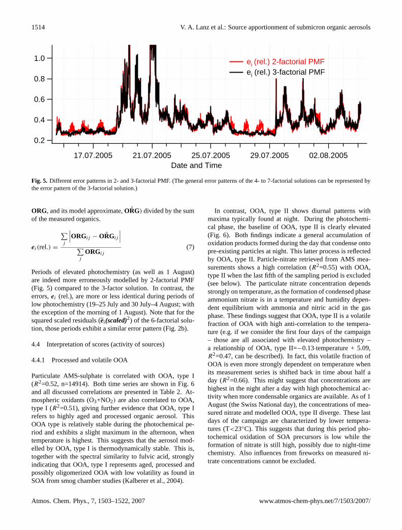
Boxplots of HOA during days dominated by commutersand heavy traffic with moderate influence of leisure trafficand activities (Monday to Friday) were calculated and com-pared to the remaining days, which can all be (partially)characterized by leisure road traffic and activities: Saturdays(after-noon and evening activities) and Sundays (trucks arebanned from roads), as well as Monday, 1 August (Swissnational holiday) (Fig. 7). For working days only, HOA ex-hibits a similar daily cycle as NOx which can be character-ized by two peaks: one in the morning at 08:00 to 09:00 a.m.and one in the evening at about 09:00 to 10:00 p.m. For theweekend and holidays, these diurnal patterns differ: not as

much in the morning, when both daily cycles do not increase(as of 05:00 a.m.), but in the evening as of 06:00 p.m., whenHOA is significantly concentrated at higher levels (comparedto morning hours). Therefore, sources other than on-roadtraffic might contribute to HOA. Note, however, that ni-trogen oxides (NOx=NO+NO2) also include substantial in-terferences by NOx oxidation products (Steinbacher et al.,2006), and are also emitted by lightning, biomass burningand industrial sources. In 2000, traffic sources contributedabout 58% of total NOx emissions in Switzerland (EKL,2005). Therefore, NOx is not a perfect traffic marker, andHOA should not be equated with pure vehicle exhaust either.

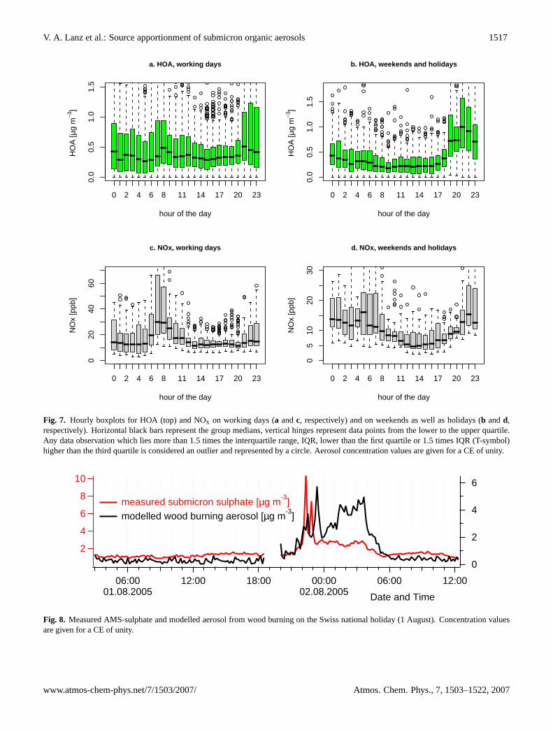
It is interesting to note the high wood burning concentra-tions compared to relatively low HOA and charbroiling con-tributions during the night from 1 August (Swiss nationalholiday) to 2 August (Fig. 6). This together with the out-standing sulphate peak is a strong indication that the woodburning factor is also influenced by emissions from the fire-works on the national holiday (fireworks consist of wood orwooden products, e.g. cardboard coating, and sulphur whichis used for several purposes). However, the peaks of sub-micron sulphate concentrations disappear rapidly while thebaseline of the modelled wood burning aerosol concentrationis still increasing until the morning increase of the bound-ary layer height. Simultaneous log-fires from upwind placesmost probably dominate the wood smoke aerosol (Fig. 8).In fact, there are lots of wood fires from big stacks at manyplaces during this evening. These fires will be smoulderingfar into the night, as actually also seen in Fig. 8.

In August 2002,14C analyses were performed by Szidat etal. (2006) at Zurich-Kaserne. Based on assumed OC/EC val-ues of wood burning for biomass emission factors they cal-culated that 13% of total organic matter stems from biomassburning. This is in good agreement with 10% wood burningcontribution calculated in this study. Based on emission in-ventories we can rule out contributions of biomass burningsources other than wood combustion. In addition, as there isvirtually no EC emission from charbroiling (shown e.g. bySchauer et al., 1999) it is unlikely that barbecue activities are



1.21.00.80.60.40.2

19.07.2005 24.07.2005 29.07.2005 03.08.2005

6

4

2

0

e. wood burning [µg m-3

] CO [ppm]

86420

19.07.2005 24.07.2005 29.07.2005 03.08.2005

d. charbroiling [µg m-3

]

30

25

20

15

19.07.2005 24.07.2005 29.07.2005 03.08.2005

2.0

1.5

1.0

0.5

0.0

5

4

3

2

1

16.07.2005 21.07.2005 26.07.2005 31.07.2005

dat

b. OOA, type II [µg m-3

] AMS particle-nitrate [µg m-3

]

temperature [°C]

4

3

2

1

019.07.2005 24.07.2005 29.07.2005 03.08.2005

10

8

6

4

2

0

a. OOA, type I [µg m-3

]

AMS particle-sulphate [µg m-3

]

10080604020

19.07.2005 24.07.2005 29.07.2005 03.08.2005

6

4

2

0

c. HOA [µg m-3

]NOx [ppb]

2.52.01.51.00.50.0

19.07.2005 24.07.2005 29.07.2005 03.08.2005

f. minor source [µg m-3

]

Fig. 6. Time series of the contributions of all identified sources and OA components as calculated by 6-factorial PMF:(a) OOA, type Iand particulate sulphate (red),(b) OOA II and particle-nitrate (blue),(c) HOA and nitrogen oxides (NOx; green),(d) charbroiling,(e) woodburning and CO (violet), and(f) minor source (possibly influenced by food cooking). Aerosol concentrations are given for a CE of unity.



0 2 4 6 8 11 14 17 20 23

0.0

0.5

1.0

1.5

hour of the day

HO

A [µ

g m

−3]

a. HOA, working days

0 2 4 6 8 11 14 17 20 23

0.0

0.5

1.0

1.5

hour of the day

HO

A [µ

g m

−3]

b. HOA, weekends and holidays

0 2 4 6 8 11 14 17 20 23

020

4060

hour of the day

NO

x [p

pb]

c. NOx, working days

0 2 4 6 8 11 14 17 20 23

05

1020

30

hour of the day

NO

x [p

pb]

d. NOx, weekends and holidays

Fig. 7. Hourly boxplots for HOA (top) and NOx on working days (a andc, respectively) and on weekends as well as holidays (b andd,respectively). Horizontal black bars represent the group medians, vertical hinges represent data points from the lower to the upper quartile.Any data observation which lies more than 1.5 times the interquartile range, IQR, lower than the first quartile or 1.5 times IQR (T-symbol)higher than the third quartile is considered an outlier and represented by a circle. Aerosol concentration values are given for a CE of unity.

10

8

6

4

2

06:0001.08.2005

12:00 18:00 00:0002.08.2005

06:00 12:00

Date and Time

6

4

2

0

measured submicron sulphate [µg m-3

] modelled wood burning aerosol [µg m

-3]

Fig. 8. Measured AMS-sulphate and modelled aerosol from wood burning on the Swiss national holiday (1 August). Concentration valuesare given for a CE of unity.



3.0

2.5

2.0

1.5

1.0

0.5

µg

m-3

201612840hour of the day

3.0

2.5

2.0

1.5

1.0

0.5

0.0

hourly medians (minor source) photochemical period whole campaign

Fig. 9. Hourly median values of the sixth factor (minor source):calculated for the photochemical phase only and for the whole cam-paign. Concentration values are given for a CE of unity.

included in this 13% biomass burning (as biomass contribu-tions were calculated from EC values).

High concentrations of charbroiling aerosols typically co-incide with evenings of periods of warm temperatures (e.g.on 14–17 July; Figs. 1 and 6). Charbroiling emissions areprobably highly variable with respect to their chemical com-position (complete and incomplete combustion of acceler-ants, char, fat) and probably cannot be described by a sin-gle mass spectrum. Therefore, we might underestimate thoseemissions here. In summertime, both charbroiling and woodburning can be expected to be due to leisure activities. It istherefore not surprising that those time series are correlated(see Fig. 6).

4.4.3 Minor source (influenced by food cooking)

Some indications that the minor source may be influencedto some extent by food cooking has been provided inSect. 4.2.5. Hourly medians were calculated for the mod-elled minor source time series and are presented in Fig. 9.An increase can observed in this factor at noon and from08:00 to 09:00 p.m. during the photochemically active peri-ods (14–18 and 26–29 July 2005; Fig. 1) which were accom-panied with anticyclonic, stable weather conditions and moreleisure activities. In contrast, there is no peak at noon and aless eminent increase in the concentration from 08:00 p.m.to 09:00 p.m. when the whole dataset is analyzed. Furtherevidence that the sixth factor can be interpreted as influencedby cooking is given by filtering the data with respect to winddirection.

4.5 Wind direction

An area of densely located restaurants (“Langstrassen-Quartier”) is in the direction of Northwest to Southwest,while air from North to East is coming from the main trainstation (“Zurich HB”). A minimal wind speed of 0.5 m/sis imposed (wind direction and wind speed are measured32.1 m above ground level). The busiest hours in that areaare typically from 06:00 p.m. to 11:00 p.m. Aerosol concen-trations from the sixth factor are significantly higher (mean:0.52µg m−3, standard deviation: 0.02µg m−3) when airfrom the “Langstrassen-Quartier” arrived at the measuringsite than when the wind came from the direction of themain train station (mean: 0.27µg m−3, standard devia-tion: 0.03µg m−3). Thus, a ratio of 1.9 can be calculatedfor aerosol from the “Langstrassen-Quartier” compared to“Zurich HB”. Note that this phenomenon is untypical forother aerosol concentrations: no significant dependence onwind direction can be observed for the other primary fac-tors (HOA, charbroiling and wood burning aerosol), and bothOOA factors are lower in air masses from West (ratio oftype I, aged fraction: 0.4; type II, volatile fraction: 0.7).Very similar results are obtained without applying the timefilter. North-eastern winds (“Bise”) during Swiss summersare typically anticyclonic and associated with clear sky andmore solar radiation favouring atmospheric oxidation pro-cesses, while Western winds often contain wet air massesfrom the Atlantic Sea. This is an indication why OOA (es-pecially type I) shows lower concentrations in Western airmasses.

4.6 Modelled emission ratios

The emission ratios of modelled primary organic aerosol(POA) or HOA versus measured primary pollutants such aselemental carbon (EC), NOx and CO are calculated from theslopes of the following linear regression modell:

POA =a + s·(measured primary pollutant) +ε (9)

Based on the solution of 6-factorial PMF, primary organicaerosol (POA) is estimated as

POA = HOA + wood burning + charbroiling + minor source(10)

Then, a ratio of 15.9µg m−3/ppmv (±2.3µg m−3/ppmv)for HOA/NOx results for this campaign. Similar valuescan be calculated from a tunnel study (Kirchstetter et al.,1999): a ratio of 16µg m−3/ppmv for diesel trucks and11µg m−3/ppmv for light-duty vehicles. In this calcula-tion, HOA as the primary component from traffic emissionwas chosen. The emission ratios calculated for the morninghours of weekends (Saturdays, Sunday and 1 August) as wellas of working days (Monday to Friday) do not significantlydiffer from the overall ratio of 15.9µg m−3/ppmv. On theother hand, values for after-noon and evening hours (12:00–23:50 p.m.) are significantly larger (s=27.7µg m−3/ppmv).



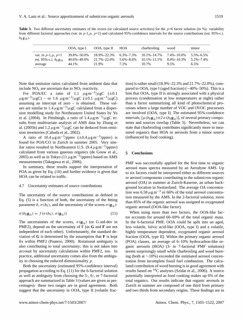
Table 3. Two different uncertainty estimates of the scores (or calculated source activities) for thep=6 factor solution (in %): variabilityfrom different factorial approaches (var. inp-1,p, p+1) and calculated 95%-confidence intervals for the source contributions (est. 95%-c.i.bkgik).

OOA, type I OOA, type II HOA charbroiling wood minor

var. inp-1,p, p+1 39.8%–50.0% 18.9%–22.3% 6.3%–7.3% 10.1%–14.7% 7.4%–10.0% 5.5%–6.5%est. 95%-c.i.bkgik 40.6%–49.0% 21.7%–22.0% 5.6%–8.6% 10.1%–11.1% 8.4%–10.3% 5.2%–7.4%average 44.1% 21.9% 7.3% 10.7% 9.5% 6.5%

Note that emission ratios calculated from ambient data thatinclude NOx are uncertain due to NO2 reactivity.

For POA/EC a ratio of 1.1 µg m−3/µgC (±0.1µg m−3/µgC) – or 1.6µg m−3/µgC (±0.1 µg m−3/µgC)assuming an intercept of zero – is obtained. These val-ues are similar to 1.4µg m−3/µgC calculated from a disper-sion modelling study for Northeastern United States by Yuet al. (2004). In Pittsburgh, a ratio of 1.4µg m−3/µgC re-sults from multivariate analysis of AMS data by Zhang etal. (2005b) and 1.2µg m−3/µgC can be deduced from emis-sion inventories (Cabada et al., 2002).

A ratio of 10.4µg m−3/ppmv (±0.4µg m−3/ppmv) isfound for POA/CO in Zurich in summer 2005. Very sim-ilar ratios resulted in Northeastern U.S. (9.4µg m−3/ppmv)calculated from various gaseous organics (de Gouw et al.,2005) as well as in Tokyo (11µg m−3/ppmv) based on AMSmeasurements (Takegawa et al., 2006).

In summary, these results support the interpretation ofPOA as given by Eq. (10) and further evidence is given thatHOA can be related to traffic.

4.7 Uncertainty estimates of source contributions

The uncertainty of the source contributions as defined inEq. (5) is a function of both, the uncertainty of the fittingparameterb, σ(bk), and the uncertainty of the scoresσ(gik):

σ(bkgik) = f (σ(bk), σ (gik)) (11)

The uncertainties of the scores,σ(gik) (or G std-dev inPMF2), depend on the uncertainty of F (asG andF are notindependent of each other). Unfortunately, the standard de-viation of G is determined by the assumption thatF is keptfix within PMF2 (Paatero, 2000). Rotational ambiguity isalso contributing to total uncertainty; this is not taken intoaccount by uncertainty calculations within PMF2, too. Inpractice, additional uncertainty comes also from the ambigu-ity in choosing the reduced dimensionalityp.

Both the uncertainty (estimated 95%-confidence interval)propagation according to Eq. (11) for the 6-factorial solutionas well as ambiguity from choosing the 5-, 6-, or 7-factorialapproach are summarized in Table 3 (values are given as per-centages): these two ranges are in good agreement. Bothsuggest that the uncertainty in OOA, type II (volatile frac-

tion) is rather small (18.9%–22.3% and 21.7%–22.0%), com-pared to OOA, type I (aged fraction) (∼40%–50%). This is ahint that OOA, type II is strongly associated with a physicalprocess (condensation at low temperatures at night) ratherthan a factor summarizing all kind of photochemical pro-cesses where a large number of VOC and OVOC precursorsare involved (OOA, type I). The estimated 95%-confidenceintervals, [µ(bkgik)±2σ(bkgik)], of several primary compo-nents and sources overlap (Table 3). Nevertheless, we canstate that charbroiling contributes significantly more to mea-sured organics than HOA or aerosols from a minor source(influenced by food cooking).

5 Conclusions

PMF was successfully applied for the first time to organicaerosol mass spectra measured by an Aerodyne AMS. Upto six factors could be interpreted either as different sourcesor aerosol components contributing to the submicron organicaerosol (OA) in summer at Zurich-Kaserne, an urban back-ground location in Switzerland. The average OA concentra-tion was 6.58µg m−3 or 66% of the total aerosol concentra-tion measured by the AMS. In the 2-factorial solution, morethan 85% of the organic aerosol was assigned to oxygenatedorganic aerosol (OOA-like factor).

When using more than two factors, the OOA-like fac-tor accounts for around 60–69% of the total organic mass.In the 6-factorial PMF, OOA could be split into an aged,less volatile, fulvic acid-like (OOA, type I) and a volatile,highly temperature dependent, oxygenated organic aerosolfraction (OOA, type II). Within the primary organic aerosol(POA) classes, an average of 6–10% hydrocarbon-like or-ganic aerosols (HOA) (3- to 7-factorial PMF solutions)seems surprisingly small while charbroiling and wood burn-ing (both at∼10%) exceeded the estimated aerosol concen-tration from incomplete fossil fuel combustion. The calcu-lated contribution of wood burning is in good agreement withresults based on14C analyses (Szidat et al., 2006). A sourcepotentially interpreted as food cooking makes up 6% of thetotal organics. Our results indicate that organic aerosols inZurich in summer are composed of one third from primaryand two thirds from secondary origins. These findings are in



line with the studies from Pittsburgh (Zhang et al., 2005b) aswell as Mexico City (Volkamer et al., 2006).

Since there are significant primary emissions of oxy-genated compounds in Zurich (∼24–27%) the 2-factorial ap-proaches overestimate the contribution of SOA by about 15–25% if the OOA-like factor is interpreted as secondary or-ganic aerosol (SOA). Note that those two PMF factors showgood agreement with measured spectra representing OOAand HOA (Alfarra, 2004; Zhang et al., 2005a), the 2-factorialsolution is associated with lowest rotational freedom and ex-plains virtually all variance of the time series of total AMS-organics. However, the OOA- and HOA-like factors from 2-factorial PMF should not be equated to SOA and POA as thedirect emission of oxygenated aerosol species from sourceslike biomass burning, charbroiling, food cooking etc. can-not be ruled out. It was shown e.g. by Simoneit et al. (1993)that emissions of those sources can include a myriad of ox-idized organic compounds. The sum of (OOA, type I) and(OOA, type II) might represent SOA but we cannot rule outthat oxidized primary particle emissions contribute to OOAin the mass spectrum. Primary biogenic emissions (e.g. waxfragments) could also be significant sources of OOA, al-though no indication was found in this study. In addition,Zurich-Kaserne might be slightly biased toward charbroil-ing and wood burning particles because of some local emis-sion events. Thus, further application of this method to otherdatasets will give more insight into the variability of thesource composition at different locations.

Acknowledgements.The AMS measurements were supportedby the Swiss Federal Office for the Environment (FOEN). Themeasurement trailer was provided by the Kanton Zurich. Wethank U. Lohmann, J. Staehelin, H. Coe, P. Paatero, and twoanonymous reviewers for valuable comments and suggestionswhich significantly improved this paper. Helpful reference spectrafrom C. Marcolli and A. M. Middlebrook, as well as fromS. Weimer and J. Schneider are greatly appreciated. We also thankJ. Allan for providing his IGOR codes, as well as J.-L. Jimenez,Q. Zhang, M. Canagaratna, I. Ulbrich, and D. R. Worsnop forcritical comments.

Edited by: T. Koop

References

Alfarra, M. R.: Insights into Atmospheric Organic Aerosols Us-ing an Aerosol Mass Spectrometer, Ph.D. thesis, Universityof Manchester Institute of Science and Technology (UMIS),Manchester, 2004.

Alfarra, M. R., Coe, H., Allan, J. D., Bower, K. N., Boudries, H.,Canagaratna, M. R., Jimenez, J. L., Jayne, J. T., Garforth, A.,Li, S.-M., and Worsnop, D. R.: Characterization of urban andregional organic aerosols in the lower Fraser Valley using twoAerodyne Aerosol Mass Spectrometers, Atmos. Environ., 38,5745–5758, 2004.

Alfarra, M. R., Paulsen, D., Gysel, M., Garforth, A. A., Dommen,J., Prevot, A. S. H., Worsnop, D. R., Baltensperger, U., and Coe,

H.: A mass spectrometric study of secondary organic aerosolsformed from the photooxidation of anthropogenic and biogenicprecursors in a reaction chamber, Atmos. Chem. Phys., 6, 5279–5293, 2006a.

Allan, J. D., Jimenez, J. L., Williams, P. I., Alfarra, M. R., Bower,K. N., Jayne, J. T., Coe, H., and Worsnop, D. R.: Quantita-tive sampling using an Aerodyne aerosol mass spectrometer –1. Techniques of data interpretation and error analysis, J. Geo-phys. Res.-Atmos., 108(D3), 4090, doi:10.1029/2002JD002358,2003.

Allan, J. D., Delia, A. E., Coe, H., Bower, K. N., Alfarra, M. R.,Jimenez, J. L., Middlebrook, A. M., Drewnick, F., Onasch, T. B.,Canagaratna, M. R., Jayne, J. T., and Worsnop, D. R.: A gen-eralised method for the extraction of chemically resolved massspectra from aerodyne aerosol mass spectrometer data, J. AerosolSci., 35, 909–922, 2004.

Bahreini, R., Keywood, M., Ng, N. L., Varutbangkul, V., Gao, S.,Flagan, R. C., Seinfeld, J. H., Worsnop, D. R., and Jimenez,J. L.: Measurements of secondary organic aerosol from oxida-tion of cycloalkanes, terpenes, and m-xylene using the AerodyneAerosol Mass Spectrometer, Environ. Sci. Technol., 39, 5674–5688, 2005.

Begum, B. A., Kim, E., Biswas, S. K., and Hopke, P. K.: Investiga-tion of sources of atmospheric aerosol at urban and semi-urbanareas in Bangladesh, Atmos. Environ., 38, 3025–3038, 2004.

Buset, K. C., Evans, G. J., Leaitch, W. R., Brook, J. R., and Toom-Sauntry, D.: Use of advanced receptor modelling for analysis ofan intensive 5-week aerosol sampling campaign, Atmos. Envi-ron., 40, Suppl. 2, 482–499, 2006.

Cabada, J. C., Pandis, S. N., and Robinson, A. L.: Sources of atmo-spheric carbonaceous particulate matter in Pittsburgh, Pennsyl-vania, J. Air Waste Manag. Assoc., 52(6), 732–741, 2002.

Cabada, J. C., Pandis, S. N., Subramanian, R., Robinson, A.L., Polidori, A., and Turpin, B.: Estimating the secondary or-ganic aerosol contribution to PM2.5 using the EC tracer method,Aerosol Sci. Technol., 38, Suppl. 1, 140–155, 2004.

Canagaratna, M. R., Jayne, J. T., Ghertner, D. A., Herndon, S.,Shi, Q., Jimenez, J. L., Silva, P. J., Williams, P., Lanni, T.,Drewnick, F., Demerjian, K. L., Kolb, C. E., and Worsnop,D. R.: Chase studies of particulate emissions from in-useNew York city vehicles, Aerosol Sci. Technol., 38, 555–573,doi:10.1080/02786820490465504, 2004.

Chung, Y. S., Kim, S. H., Moon, J. H., Kim, Y. J., Lim, J. M.,and Lee, J. H.: Source identification and long-term monitoringof airborne particulate matter PM2.5/PM10) in an urban regionof Korea, J. Radioanal. Nucl. Chem., 267, 35–48, 2005.

de Gouw, J. A., Middlebrook, A. M., Warneke, C., Goldan, P.D., Kuster, W. C., Roberts, J. M., Fehsenfeld, F. C., Worsnop,D. R., Canagaratna, M. R., Pszenny, A. A. P., Keene, W. C.,Marchewka, M., Bertman, S. B., and Bates, T. S.: Budget oforganic carbon in a polluted atmosphere: Results from the NewEngland Air Quality Study in 2002, J. Geophys. Res.-Atmos.,110, D16305, doi:10.1029/2004JD005623, 2005.

EKL: Status-Bericht der Eidg. Kommission fur Lufthygiene.Stickstoffhaltige Luftschadstoffe in der Schweiz, SchriftenreiheUmwelt Nr. 384, Herausgegeben vom Bundesamt fur Umwelt,Wald und Landschaft BUWAL, Bern, 2005.

Empa: Technischer Bericht zum Nationalen Beobachtungsnetz furLuftfremdstoffe (NABEL), available at:http://www.empa.ch/


http://www.empa.ch/nabel


nabel, Dubendorf, Switzerland, 2005.Fuzzi, S., Andreae, M. O., Huebert, B. J., Kulmala, M., Bond,

T. C., Boy, M., Doherty, S. J., Guenther, A., Kanakidou, M.,Kawamura, K., Kerminen, V.-M., Lohmann, U., Russell, L. M.,and Pschl, U.: Critical assessment of the current state of scien-tific knowledge, terminology, and research needs concerning therole of organic aerosols in the atmosphere, climate, and globalchange, Atmos. Chem. Phys., 6, 2017–2038, 2006,http://www.atmos-chem-phys.net/6/2017/2006/.

Hedberg, E., Gidhagen, L., and Johansson, C.: Source contributionsto PM10 and arsenic concentrations in Central Chile using posi-tive matrix factorization, Atmos. Environ., 39, 549–561, 2005.

Hien, P. D., Bac, V. T., and Thinh, N. T. H.: PMF receptor mod-elling of fine and coarse PM10 in air masses governing mon-soon conditions in Hanoi, Northern Vietnam, Atmos. Environ.,38, 189–201, 2004.

Hopke, P. K: Recent developments in receptor modeling, J.Chemom., 17, 255–265, 2003.

Huang, S., Rahn, K. A., and Arimoto, R.: Testing and optimizingtwo factor-analysis techniques on aerosol at Narragansett, RhodeIsland, Atmos. Environ., 33, 2169–2185, 1999.

Horvath, H.: Atmospheric light-absorption – A review, Atmos. En-viron. Part A-General Topics, 27, 293–317, 1993.

Jaffrezo, J.-L., Aymoz, G., and Cozic, J.: Size distribution of ECand OC in the aerosol of Alpine valleys during summer and win-ter, Atmos. Chem. Phys., 5, 2915–2925, 2005,http://www.atmos-chem-phys.net/5/2915/2005/.

Jayne, J. T., Leard, D. C., Zhang, X. F., Davidovits, P., Smith, K.A., Kolb, C. E., and Worsnop, D. R.: Development of an aerosolmass spectrometer for size and composition analysis of submi-cron particles, Aerosol Sci. Technol., 33, 49–70, 2000.

Jenkin, M. E., Saunders, S. M., Wagner, V., and Pilling, M. J.: Pro-tocol for the development of the Master Chemical Mechanism,MCM v3 (Part B): tropospheric degradation of aromatic volatileorganic compounds, Atmos. Chem. Phys., 3, 181–193, 2003,http://www.atmos-chem-phys.net/3/181/2003/.

Jimenez, J.-L., Jayne, J. T., Shi, Q., Kolb, C. E., Worsnop, D. R.,Yourshaw, I., Seinfeld, J. H., Flagan, R. C., Zhang, X. F., Smith,K. A., Morris, J. W., and Davidovits, P.: Ambient aerosol sam-pling using the Aerodyne Aerosol Mass Spectrometer, 108(D7),8425, doi:10.1029/2001JD001213, 2003.

Kalberer, M., Paulsen, D., Sax, M., Steinbacher, M., Dommen, J.,Prevot, A. S. H., Fisseha, R., Weingartner, E., Frankevich, V.,Zenobi, R., and Baltensperger, U.: Identification of polymersas major components of atmospheric organic aerosols, Science,303, 1659–1662, 2004.

Kanakidou, M., Seinfeld, J. H., Pandis, S. N., Barnes, I., Dentener,F. J., Facchini, M. C., van Dingenen, R., Ervens, B., Nenes, A.,Nielsen, C. J., Swietlicki, E., Putaud, J. P., Balkanski, Y., Fuzzi,S., Horth, J., Moortgat, G. K., Winterhalter, R., Myhre, C. E.L., Tsigaridis, K., Vignati, E., Stephanou, E. G., and Wilson, J.:Organic aerosol and global climate modelling: a review, Atmos.Chem. Phys., 5, 1053–1123, 2005,http://www.atmos-chem-phys.net/5/1053/2005/.

Katrib, Y., Martin, S. T., Hung, H. M., Rudich, Y., Zhang, H. Z.,Slowik, J. G., Davidovits, P., Jayne, J. T., and Worsnop, D. R.:Products and mechanisms of ozone reactions with oleic acid foraerosol particles having core-shell morphologies, J. Phys. Chem.,A 108, 6686–6695, 2004.

Kim, E., Hopke, P. K., and Edgerton, E. S.: Source identificationof Atlanta aerosol by positive matrix factorization, J Air WasteManage. Assoc., 53, 731–739, 2003.

Kim, E. and Hopke, P. K.: Identification of fine particle sourcesin mid-Atlantic US area, Water Air Soil Pollut., 168, 391–421,2005.

Kirchstetter, T., Harley, R., Kreisberg, N., Stolzenburg, M., andHering, S.: On-road measurement of fine particle and nitrogenoxide emissions from light- and heavy-duty motor vehicles, At-mos. Environ., 33(18), 2955–2968, 1999.

Lee, E., Chun, C. K., and Paatero, P.: Application of Positive MatrixFactorization in Source Apportionment of Particulate Pollutants,Atmos. Environ., 33, 3201–3212, 1999.

Li, Z., Hopke, P. K., Husain, L., Qureshi, S., Dutkiewicz, V. A.,Schwab, J. J., Drewnick, F., and Demerjian, K. L.: Sources offine particle composition in New York city, edited by: Li, Z.,Hopke, P. K., and Husain, L., Atmos. Environ., 38, 6521–6529,2004.

Liu, W., Hopke, P. K., and VanCuren, R. A.: Origins of fineaerosol mass in the western United States using positive ma-trix factorization, J. Geophys. Res.-Atmos., 108(D23), 4716,doi:10.1029/2003JD003678, 2003.

Lohmann, U. and Feichter, J.: Global indirect aerosol effects: areview, Atmos. Chem. Phys., 5, 715–737, 2005,http://www.atmos-chem-phys.net/5/715/2005/.

Nel, A.: Air pollution-related illness: effects of particles, Science,308, 804–806, 2005.

NIST: National Institute of Standards and Technology, NIST Chem-istry WebBook, available at:http://webbook.nist.gov/chemistry,July 2006.

Paatero, P.: Least squares formulation of robust non-negative factoranalysis, Chemom. Intell. Lab. Syst., 37, 23–35, 1997.

Paatero, P.: User’s guide for positive matrix factorization programsPMF2.EXE and PMF3.EXE, University of Helsinki, Finland,2000.

Paatero, P: User’s guide for positive matrix factorization programsPMF2 and PMF3, part 1: tutorial, University of Helsinki, Fin-land, 2007.

Paatero, P. and Tapper, U.: Positive matrix factorization: a non-negative factor model with optimal utilization of error estimatesof data values, Environmetrics, 5, 111–126, 1994.

Pekney, N. J., Davidson, C. I., Robinson, A., Zhou, L., Hopke,P., Eatough, D., and Rogge, W. F.: Major source categories forPM2.5 in Pittsburgh using PMF and UNMIX, Aerosol Sci. Tech-nol., 40, 910–924, 2006.

Quinn, P. K., Bates, T. S., Coffman, D., Onasch, T. B., Worsnop,D., Baynard, T., de Gouw, J. A., Goldan, P. D., Kuster, W.C., Williams, E., Roberts, J. M., Lerner, B., Stohl, A., Pet-tersson, A., and Lovejoy, E. R.: Impacts of sources and ag-ing on submicrometer aerosol properties in the marine boundarylayer across the Gulf of Maine, J. Geophys. Res., 111, D23S36,doi:10.1029/2006JD007582, 2006.

Ramadan, Z., Song, X. H., and Hopke, P. K.: Identification ofsources of Phoenix aerosol by positive matrix factorization, J.Air Waste Manage. Assoc., 50, 1308–1320, 2000.

Schauer, J. J., Rogge, W. F., Hildemann, L. M., Mazurek, M. A.,Cass, G. R., and Simoneit, B. R. T.: Source apportionment ofairborne particulate matter using organic compounds as tracers,Atmos. Environ., 30, 3837–3855, 1996.


http://www.empa.ch/nabel

http://www.atmos-chem-phys.net/6/2017/2006/





http://webbook.nist.gov/chemistry


Schauer, J. J., Kleeman, M. J., Cass, G. R., and Simoneit, B. R.T.: Measurement of emissions from air pollution sources. 1. C1through C29 organic compounds from meat charbroiling, Envi-ron. Sci. Technol., 33, 1566–1577, 1999.

Schneider, J., Weimer, S., Drewnick, F., Borrmann, S., Helas, G.,Gwaze, P., Schmid, O., Andreae, M. O., and Kirchner, U.: Massspectrometric analysis and aerodynamic properties of varioustypes of combustion-related aerosol particles, Int. J. Mass. Spec.,258, 37–49, 2006.

Simoneit, B. R. T., Rogge, W. F., Mazurek, M. A., Standley, L. J.,Hildemann, L. M., and Cass, G. R.: Lignin pyrolysis products,lignans, and resin acids as specific tracers from biomass combus-tion, Environ. Sci. Technol., 27, 2533–2540, 1993.

Song, X. H., Polissar, A. V., and Hopke, P. K.: Sources of fineparticle composition in the northeastern US, Atmos. Environ.,35, 5277–5286, 2001.

Steinbacher, M., Zellweger, C., and Schwarzenbach, B.: Nitrogenoxides measurements at rural sites in Switzerland: bias of con-ventional measurement techniques, J. Geophys. Res., accepted,2007.

Szidat, S., Jenk, T. M., Synal, H.-A., Kalberer, M., Wacker, L., Haj-das, I., Kasper-Giebl, A., and Baltensperger, U.: Contributions offossil fuel, biomass-burning, and biogenic emissions to carbona-ceous aerosols in Zurich as traced by 14C, J. Geophys. Res., 111,D07206, doi:10.1029/2005JD006590, 2006.

Takegawa, N., Miyakawa, T., Kondo, Y., Jimenez, J. L., Zhang, Q.,Worsnop, D. R., and Fukuda, M.: Seasonal and diurnal variationsof submicron organic aerosol in Tokyo observed using the Aero-dyne aerosol mass spectrometer, J. Geophys. Res., 111, D11206,doi:10.1029/2005JD006515, 2006.

Turpin, B. J. and Huntzicker, J. J.: Identification of secondary or-ganic aerosol episodes and quantification of primary and sec-ondary organic aerosol concentrations during SCAQS, Atmos.Environ., 29, 3527–3544, 1995.

Volkamer, R., Jimenez, J. L., San Martini, F., Dzepina, K., Zhang,Q., Salcedo, D., Molina, L. T., Worsnop, D. R., and Molina, M.J.: Secondary organic aerosol formation from anthropogenic airpollution: rapid and higher than expected, Geophys. Res. Lett.,33, L17811, doi:10.1029/2006GL026899, 2006.

Yu, S., Dennis, R. L., Bhave, P. V., and Eder, B. K.: Primary andsecondary organic aerosols over the United States: estimates onthe basis of observed organic carbon (OC) and elemental carbon(EC), and air quality modeled primary OC/EC ratios, Atmos. En-viron., 38(31), 5257–5268, 2004.

Yuan, Z. B., Lau, A. K. H., Zhang, H. Y., Yu, J. Z., Louie, P. K. K.,and Fung, J. C. H.: Identification and spatiotemporal variationsof dominant PM10 sources over Hong Kong, Atmos. Environ.,40, 1803–1815, 2006.

Zhang, Q., Alfarra, M. R., Worsnop, D. R., Allan, J. D., Coe, H.,Canagaratna, M. R., and Jimenez, J. L.: Deconvolution and quan-tification of hydrocarbon-like and oxygenated organic aerosolsbased on aerosol mass spectrometry, Environ. Sci. Technol., 39,4938–4952, 2005a.

Zhang, Q., Worsnop, D. R., Canagaratna, M. R., and Jimenez, J. L.:Hydrocarbon-like and oxygenated organic aerosols in Pittsburgh:insights into sources and processes of organic aerosols, Atmos.Chem. Phys., 5, 3289–3311, 2005b.

Zhao, W. X. and Hopke, P. K.: Source identification for fineaerosols in Mammoth Cave National Park, Atmos. Res., 80, 309–322, 2006.


source apportionment of submicron organic aerosols at an urban

Documents