soil fertility: quefts and farmers’ perceptionspubs.iied.org/pdfs/8138iied.pdf · soil fertility:...
TRANSCRIPT

Soil Fertility: QUEFTS and Farmers’ Perceptions Ingrid Mulder Working Paper No 30 July 2000
International Institute for Environment and Development, London and Institute for Environmental Studies, Amsterdam

Author Ingrid Mulder is Assistant Researcher at the Faculty of Economic Sciences, Vrije Universiteit. She may be contacted at: Section Economics and Development Economics Faculty of Economic Sciences, Business Administration and Econometrics Vrije Universiteit De Boelelaan 1105 1081 HV Amsterdam The Netherlands Tel: + 31 20 444 6142; Fax: + 31 20 444 6004; email: [email protected]

The programme of Collaborative Research in the Economics of Environment and Development (CREED) was established in 1993 as a joint initiative of the International Institute for Environment and Development (IIED), London, and the Institute for Environmental Studies (IVM), Amsterdam. The Secretariat for CREED is based at IIED in London. A Steering Committee is responsible for overall management and coordination of the CREED Programme. Environmental Economics Programme, IIED IIED is an independent, non-profit organisation which seeks to promote sustainable patterns of world development through research, training, policy studies, consensus building and public information. The Environmental Economics Programme is one of seven major programmes of IIED; it conducts economic research and policy analysis for improved management of natural resources and sustainable economic growth in the developing world.
Environmental Economics Programme IIED, 3 Endsleigh Street London WC1H 0DD, UK Tel +44 (0)171 388 2117; Fax +44 (0)171 388 2826 e-mail: [email protected]
Institute for Environmental Studies, (IVM) IVM is a non-profit research institute, based at Vrije Universiteit, Amsterdam. The Institute's primary objective is to carry out multi- and interdisciplinary research on environmental issues, based on cross-fertilisation of monodisciplinary sciences. Environment and the Third World is one of eight major IVM research programmes.
IVM, Vrije Universiteit De Boelelaan 1115 1081 HV Amsterdam The Netherlands Tel: +31 20 444 9555; Fax: +31 20 444 9553 e-mail:[email protected]
CREED Steering Committee members include:
Prof Johannes Opschoor, Institute for Social Studies, The Netherlands (Chair) Prof Gopal Kadekodi, Centre for Multidisciplinary Development Research, India Dr Ronaldo Seroa da Motta, IPEA, Brazil Dr Mohamud Jama, Institute for Development Studies, Kenya Dr Anantha K Duraiappah, IVM, The Netherlands Prof Harmen Verbruggen, IVM, The Netherlands Joshua Bishop, IIED, UK Maryanne Grieg-Gran, IIED, UK
This paper is available on the CREED web site at:
http://www.iied.org/creed

Acknowledgements This paper draws heavily on Janssen et al.(1990) and Smaling (1993). I would like to thank Dr. Ir. B.H. Janssen for allowing me the use of the QUEFTS software. I would also like to thank Dr. Ir. B.H. Janssen and Dr. J. Wolf and an anonymous referee for their useful comments.

Abstract Soil fertility is one of many factors which influence farmers’ choices regarding agricultural production, fertilisation and soil and water conservation. Before we can study the effects however, we need to measure soil fertility. We use the QUEFTS model (QUantitative Evaluation of the Fertility of Tropical Soils - Janssen et al., 1990), which predicts crop yields from chemical soil characteristics, as an indicator of soil fertility. We then compare these predictions with actual yields as well as farmers’ own estimates of soil fertility. The results of QUEFTS for the soil samples taken in the Atacora region in Benin show that Nitrogen is the most limiting nutrient in the sample zone, while Phosphorus and Potassium are in quite ample supply. Potassium could be limiting, especially for legumes. QUEFTS yields are much higher than and not correlated to actual yields obtained by farmers. This implies that soil fertility is one of many limiting factors in the central zone of the Atacora. Others include, eg, availability of labour and access to a plough. Knowing how limiting soil fertility actually is requires the estimation of a more general model that includes these other inputs. When we compare QUEFTS yields to farmers’ own estimates of soil fertility we find no correlation. Farmers’ estimates seem to be based on very different aspects of soil fertility other than nutrient content than QUEFTS. Résumé La fertilité pédologique est un des nombreux facteurs qui pèsent sur les choix des paysans en matière de production agricole, d'amendement des terres et de conservation des sols et de l'eau. Mais avant de pouvoir en étudier les effets, il nous faut mesurer la fertilité des sols. Nous avons employé pour ce faire le modèle QUEFTS (QUantitative Evaluation of the Fertility of Tropical Soils [Évaluation quantitative de la fertilité des sols tropicaux]—Janssen et al., 1990), qui permet de prévoir les rendements culturaux à partir des caractéristiques chimiques des sols, prises comme indicateurs de la fertilité pédologique. Nous comparons ensuite ces prévisions aux rendements réellement obtenus ainsi qu'aux estimations de la fertilité pédologique établies par les agriculteurs eux-mêmes. En ce qui concerne les échantillons de sols prélevés dans la région de l'Atacora au Bénin, les résultats de QUEFTS montrent que l'azote est l'élément nutritif les plus limitatif de la zone de prélèvement, alors qu'on y trouve d'amples proportions de phosphore et de potassium. Ce dernier pourrait s'avérer limitatif, surtout en ce qui concerne les légumineuses. Les rendements obtenus par QUEFTS sont de beaucoup supérieurs à, et sans corrélation avec, les rendements réels obtenus par les cultivateurs, ce qui implique que la fertilité pédologique n'est qu'un parmi d'autres facteurs limitatifs rencontrés dans la zone centrale de l'Atacora (ex.: main d'œuvre disponible, accès à une charrue). Pour savoir dans quelle mesure la fertilité pédologique est vraiment limitative, il est nécessaire de disposer de l'estimation fournie par un modèle d'ordre plus général, prenant en compte ces autres intrants. Faisant la comparaison des rendements QUEFTS et des estimations, par les agriculteurs eux-mêmes, de la fertilité des sols, nous n'avons trouvé aucune corrélation. Les estimations paysannes semblent reposer sur des aspects de la fertilité pédologique très différents des proportions d'éléments nutritifs présents dans le sol, et très différents aussi de ce que retient pour ses calculs le modèle QUEFTS.
Resumen La fertilidad del suelo es uno de los muchos factores que influyen sobre las opciones de los agricultores con relación a la producción agrícola, la fertilización y la conservación del suelo y de las aguas. Antes de evaluar dichos factores es necesario medir la fertilidad del suelo. Se utiliza un

modelo que permite predecir el rendimiento de las cosechas a partir de la composición química del suelo como indicador de su fertilidad. El modelo se denomina ECFST (Evaluación cuantitativa de la fertilidad de suelos tropicales; Janssen et al., 1990). Los resultados de aplicar ECFST a muestras de suelo tomadas en la región de Atacora, en Benin, revelan que existe una escasez de nitrógeno, en tanto que el fósforo y el potasio son abundantes. El potasio puede limitar el crecimiento, especialmente de las legumbres. El rendimiento que se obtiene con ECFST es mucho más alto y no está correlacionado con los rendimientos reales de los agricultores. Esto demuestra que la fertilidad del suelo es una de las limitaciones en la zona central de Atacora. Otras limitaciones son, por ejemplo, la disponibilidad de trabajo manual y el acceso a arados. Para evaluar las limitaciones impuestas por la fertilidad del suelo es necesario desarrollar un modelo más general que incluya estos otros factores. Al comparar el rendimiento de los ECFST con los cálculos de fertilidad del suelo de los agricultores no se encuentra ninguna correlación. En comparación con ECFST, los cálculos de los agricultores parecen basarse en aspectos de fertilidad distintos al contenido de nutrientes en el suelo.

Contents
Introduction 1 Soil fertility 3 Processes in the soil 3 Nutrients in the soil 5 Yield response laws 7 Crop growth models 9 QUEFTS – model description 10 Validity of QUEFTS for Atacora 20 Boundary values of soil properties 20 Supply curves and outliers 21 QUEFTS results and most limiting nutrients 23 QUEFTS for different crops 23 Modified v original version 24 QUEFTS results by village and land use 27 Villages 27 Cultivation periods and fallow 28 Crop choice 29 QUEFTS yields and farmers’ yields 33 Farmers perceptions of fertility 35 Conclusion 39 Bibliography 41 Annexes 43


CREED Working Paper Series No 30 1
Introduction The productivity of agricultural land is affected by a range of factors. Some, such as climate (including rainfall, evaporation, solar radiation, temperature and wind) are beyond farmers’ control. Others however, such as soil fertility, are more influenced by farmers’ past and present activities. Soil fertility both affects and is affected by the choices that farmers make regarding agricultural production, fertilisation, and soil and water conservation regimes. In order to study these affects we need a method for measuring soil fertility. Unfortunately, there is no unique technique. Fertility is not a distinct property of the soil as such, since many soil properties influence fertility and also influence each other. Ultimately, farmers are not interested in the soil properties themselves, but how they affect agricultural production. We can therefore use models to explain the effects on yields of individual soil properties that are measured by soil sampling. The predicted yield can then be used as an indicator of soil fertility. Janssen et al.(1990) describe such a model in QUEFTS (QUantitative Evaluation of the Fertility of Tropical Soils). QUEFTS predicts crop yields from chemical soil characteristics, assuming all other production factors are optimal. While the assumption may not be realistic, QUEFTS can still be used as an indicator of soil fertility.
As a part of a larger survey held May to July 1996, soil samples were taken from 295 plots in the centre zone of the Atacora province in the north-west of Benin. The Atacora region covers almost one third of the surface of Benin (see Figure 1). With only 21 inhabitants per km2, the Atacora is the most sparsely populated region in Benin after the Borgou. Its population is largely agricultural (92%). In 1992, 77,289 agricultural households were registered with an average size of 7.6 persons per household (INSAE, 1994). On average, 4 workers are available per farm. Around 47% of the total area is suitable for agriculture. Per agricultural household this amounts to 19 ha of arable land (MDR, 1993) of which no more than 2.37 ha are cultivated (MDR/DAPS, 1995). There are large differences in population density within the Atacora.
The area from which the soil samples were taken included Copargo, Ouaké and Natitingou. The climate is Sudanian with an annual rainfall of between 1200 and 1300 mm. The tropical ferruginous soils are often pebbly but profound and have a moderate fertility. The soils are sensitive to leaching. The ecosystem in this region is one of tree savannah evolving into a bush savannah. The main crops grown are yam, sorghum and millet.
The purpose of this paper is to present the results of the soil samples in a useful way using QUEFTS. Specifically, the aim of the survey was to identify the most limiting nutrients in the sample zone, and how limiting soil fertility is in the area and the individual villages. Moreover we would like to show the effect of soil fertility decline over the years a plot is in cultivation and how soil fertility influences crop choice.

CREED Working Paper Series No 30 2
Figure 1 The VU-UNB survey area 1996
In addition to using a measure of soil fertility based on soil properties, we can ask farmers to indicate the soil fertility of each plot. Although this subjective measure makes it difficult to compare plots of different farmers, for economic applications such as the estimation of production functions, it could be sufficient while requiring far less time and resources. Our survey allowed the use of both methods and they will be discussed and compared in this paper. Section 2 clarifies the concept of soil fertility. In this section the function of nutrients in the soil and the relationship between nutrient uptake and crop yield according to agronomic laws is explained. The QUEFTS model is explained in detail in Section 3 together with its extensions. QUEFTS was tested under certain boundary conditions for the soil properties. We will discuss how restrictive these boundary conditions are for the central zone of the Atacora. We will motivate the choice for the nutrient supply curves used in the remainder of the paper. The results of QUEFTS are presented for two versions of the model and for the model adjusted for specific crops. We look at how yield estimates are correlated and what nutrients are limiting according to the different versions. We then revert to the household survey of the central zone. We compare QUEFTS results of different plots, where these plots are classified according to village, crop choice or cultivation period. We compare QUEFTS yields to actual yields obtained in the survey area. Finally, we compare QUEFTS results with the farmers’ estimates of fertility. The conclusions are drawn in the final section.

CREED Working Paper Series No 30 3
Soil Fertility
Processes in the soil A soil’s fertility depends on its chemical and structural properties such as acidity, organic matter content, characteristics as a rooting medium and abilities to hold nutrients and water. We are especially interested in the chemical degradation of soil as a result of agricultural production, also called soil mining. We therefore focus on chemical soil fertility, ie the fertility as explained by the chemical composition of the soil. Soil fertility in our study is defined as the capacity of a soil to provide plants with nutrients. To get a better understanding of where these nutrients come from, we will explain the main processes in the soil. Soil consists of disintegrated rock particles, water, air, organic matter (humus) and living organisms (Operations Review Unit, 1995). It is not a static substance, but it is constantly influenced by physical, chemical and biological processes (see Figure 2). In the soil, nutrients are available that are essential for plant growth. Small quantities of nutrients are absorbed from the atmosphere or the falling rain, but most nutrients are taken from the soil. Nutrients are present in the soil in the following forms:
(i) Nutrients in the soil moisture, made available from the mineralisation of organic matter
and weathering of mineral reserves in the soil. (ii) Nutrients present in the soil organic matter. (iii) Nutrients reserves contained in minerals (rocks and the rock-like deposits) (iv) Nutrients absorbed by minerals and organic matter - the adsorption complex These nutrients present in the soil are not directly available to the plant, except for the nutrients in the soil moisture (form i).
Soil is formed by the physical and chemical breakdown of rock and rock-like deposits or soil minerals (form iii), under the influence of the climate. This process is called weathering (Gibbon and Pain, 1985). Through weathering of soil minerals, nutrients are released in a form that can be taken up by the plant (form i). Weathering is a very slow process. In tropical soils, weatherable minerals have been degraded to clay minerals with a low capacity to adsorb and supply nutrients. Organic matter (form ii) is formed from the remains of dead plants that decompose in the soil through biological processes. The soil organic matter is further broken down. This change from an organic form to an inorganic form by microbial decomposition is called mineralisation (Fitzpatrick, 1986). Through mineralisation, nutrients become available to be taken up by plants (form i).

CREED Working Paper Series No 30 4
SOIL
availablenutrients
organic material
mineralreserves mineralisation
weathering
deposition N-fixation sedimentation groundwater
rise fertilisation
IN
erosion leachingharvested
productgaseous
losses
OUT
Note: Based on Van der Pol (1992)
Figure 2 The soil and its nutrient flows
The adsorption complex (form iv) is a source of positively charged nutrients (cations) like K+, Ca2+ and Mg2+. The negative charges on the large surface of clay and humus bind positively charged nutrients. The Cation Exchange Capacity (CEC) measures this ability of a soil to hold positively charged ions. The CEC is partly permanent and partly dependent on the soil pH. The CEC can be subdivided in an organic (humus-organic matter) and an inorganic (clay) part. There is a fairly constant equilibrium between the adsorbed cations and those freely available in the soil moisture (Euroconsult, 1989). The soil organic matter is built up over the many years that the land has been under natural vegetation. When the land is cleared and is cultivated without using fertilisers, the natural fertility decreases over time. Fallow periods are then needed to recover the soil fertility, through mineralisation, weathering, atmospheric deposition, biological fixation and, particularly, for recycling of nutrients from deeper soil horizons by roots1, where long fallow period are necessary to allow crops with a deep rooting system to establish themselves. The kind of vegetation that will grow during a natural fallow depends on its duration and the area. With increasing fallow length we can generally identify grass, bush and tree fallow. The length of the fallow period needed to restore soil fertility varies greatly according to climate and soil type. Through these processes nutrients that once originated from soil minerals, are recycled and accumulated through organic matter. 1 A soil horizon is a layer in the soil.

CREED Working Paper Series No 30 5
Since weathering of soil minerals is a relatively slow process, the nutrients available to the plant in unfertilised soils stem mainly from the soil organic matter (Bradshaw and Chadwick, 1980). Nutrients can also be made available to plants by applying (mineral) fertilisers – this adds to the forms (i), (ii) and (iv) above.
The physical, chemical and biological processes mentioned above are accelerated by high temperature and rainfall. Consequently, soils both form and degrade more quickly in tropical than in temperate zones (Operations Review Unit, 1995). This means that in tropical zones soil fertility is more difficult to maintain. The main characteristics of tropical soils are (Van Reuler and Prins, 1993):
! low content of weatherable minerals; ! high content of iron/aluminium compounds; ! high acidity (low pH); ! clay minerals with a low capacity to absorb nutrients; ! low organic matter contents.
In tropical soils, the weatherable minerals have been degraded to clay minerals (kaolinite) with a low capacity to absorb and supply nutrients. Soil (containing nutrients) can also be formed elsewhere and deposited by wind and water; similarly it can also be taken away – a process called erosion. This soil ends up elsewhere through depositing and sedimentation. This is important because the amount of soil is also important. In some areas the soil layer can be very shallow, which means that smaller quantities of nutrients can be taken up by a plant compared to a deeper soil, depending on the rooting depth.
We can conclude there is a difference between the total amount of nutrients present in the soil (potential fertility) and the amount of nutrients that can be taken up by the plant (actual fertility). Actual fertility refers to the capacity of the soil to supply nutrients from its inorganic and organic reserves through the processes of weathering and mineralisation. Potential fertility, however, refers to the total amount of nutrients that may become available to the crop in the long term (Euroconsult, 1989).
The actual soil fertility can be determined by extracting specific nutrients from the soil with mild extractants and using the composition of the extracts as a fertility criterion (Euroconsult, 1989). However, the ability of plants to absorb the nutrients from the soil depends on certain soil characteristics such as the soil’s acidity (pH), which is not the equivalent for all nutrients. A higher pH may have a positive influence on the availability of one nutrient and a negative influence on another. In addition, plants differ in their ability to mobilise and utilise nutrients from a given soil (Euroconsult, 1989). Consequently, there is no unique way of measuring soil fertility.

CREED Working Paper Series No 30 6
Nutrients in the soil There are many different nutrients in the soil, all having their own specific function for the plant. In this section we will discuss the main nutrients and their functions. Apart from carbon, hydrogen and oxygen, plants need nutrients that can be subdivided in two groups (Operations Review Unit, 1995): ! Macro-nutrients: nitrogen (N), phosphorus (P) and potassium (K), sulphur (S), calcium
(Ca) and magnesium (Mg); ! Micro-nutrients (trace-elements): iron (Fe), manganese (Mn), zinc (Zn), copper (Cu),
boron (B), molybdenum (Mo) and chlorine (Cl). The nutrients needed in larger amounts include nitrogen, phosphorus and potassium, and are referred to as the primary nutrient elements. These are followed by the other macro-nutrients, sulphur, calcium and magnesium (secondary nutrient elements). While the micro-nutrients are needed in small quantities, their presence in the soil is important. In this study we will only consider the three primary nutrient elements, which are discussed in more detail below. Nitrogen Nitrogen (N) is an important component of proteins, and thus of plant tissue. The main source of nitrogen in unfertilised soils is the soil organic matter, where it is present in the form of organic N. Organic matter is decomposed by bacteria and fungi, which transfers the organic N into ammonia and eventually into nitrate (NO3
-) which can be taken up by the plant roots. In this form it is highly mobile and in the rainy season nitrogen is easily leached. Leaching is the flow of nutrients to soil layers below the rooting zone. As a result, soil nitrates show large seasonal variations (Bradshaw and Chadwick, 1980). Measurement of total nitrogen in the soil therefore does not necessarily give a good indication of soil nitrogen that can be taken up by the plant (Gibbon and Pain, 1985). Certain plants, particularly legumes, have a symbiotic relationship with certain bacteria that enter their roots, form nodules and fix nitrogen from the atmosphere. This property is often used to enhance soil fertility. According to Gibbon and Pain (1985), the residual N contribution from annual legumes to crops grown the following season appears to be minimal. The residual from cultivation of perennial leguminous trees and bushes is probably lost or used during the first year of cultivation after clearance. However, there is some evidence that cereals benefit from the nitrogen fixed by leguminous plants when intercropped.
Phosphorus Phosphorus (P) plays an important role in the setting of fruit and seeds. It is present in the soil in three ways: a labile form, a stable form and the mineral reserve. Phosphorus is usually present in the soil as phosphate, and only partly soluble and not very mobile. Phosphate binds easily with various components of the soil, resulting in iron and aluminium phosphates in acid soils and calcium phosphates in alkaline soils. When bound in these ways, phosphorus becomes less soluble which means that it is less easily released to become available to plants. Phosphorus in this bound form is referred to as phosphorus in the stable pool. This means that in most soils only a small portion of the phosphorus in the soil is in a form that can be easily taken up by plants (the labile pool). Both the stable and the labile

CREED Working Paper Series No 30 7
pool consist of inorganic and organic forms of P (Wolf et al., 1987). In the soil a certain exchange of phosphorus between the stable and the labile pool takes place, rendering P either more or less available to plants. A well-developed rooting system is needed for the plant to be able to take up sufficient phosphorus from the soil. The last source, phosphorus originating from the soil minerals, becomes available through weathering. When taking account of the time scale of this process, the rate of this input can be considered constant (Wolf et al., 1987).
The fact that phosphorus is not very mobile also holds for phosphorus added to the soil (Bradshaw and Chadwick, 1980). This means that phosphates added in one season are recovered to a limited extent in the first cropping year, but will be released in the following years as well.
Potassium Potassium (K) is an element that influences the uptake of other elements and affects respiration and transpiration of the plant (Fitzpatrick, 1986). Potassium in the soil is usually in a form that can be easily taken up by the plant. An important property of soil that influences the availability of potassium to the plant is the soil’s adsorption complex measured by the CEC. Yield response laws We now need to examine how much and in what proportion the plant needs these nutrients and how nutrient supply influences yields. Two important agronomic laws tell us something about the nature of these relationships: Liebig’s law of the minimum and Liebscher’s law of the optimum. Although they are referred to as ‘laws’, they cannot be considered as strict physical laws; moreover they are more or less conflicting.
Liebig’s law of the minimum states that the yield of a crop is proportional to the supply of that element that is essential for the development of the crop, and that is available in relatively the smallest amount (de Wit, 1992). This proportion is independent of the supply of the other nutrients. The law of the minimum can be interpreted as follows: each nutrient has its own specific functions in the plant and cannot be substituted by other nutrients. In economic theory this would be equivalent to a Leontief technology.
Liebig’s law is often associated with the law of diminishing marginal returns, but in a strict sense the two are not equivalent. Liebig’s law implies that the marginal returns to a nutrient are constant as long as the nutrient is limiting and the marginal returns are zero when the nutrient is no longer limiting. A technology can also exhibit diminishing marginal returns when Liebig’s law does not hold. For instance when nutrients can be substituted, they can still exhibit diminishing marginal returns. Liebscher’s law of the optimum states that a production factor that is in minimum supply contributes more to production the closer other production factors are to their optimum2. This means that the marginal returns of one nutrient also depend on the supply of other nutrients,
2 This law refers to production factors in a broad sense, not only to nutrients.

CREED Working Paper Series No 30 8
and not only the most limiting one. This also means a certain substitution is possible between different nutrients. In a figure we could depict the two laws as follows (Figure 3). Curve A shows the marginal response curve according to the law of the minimum. As long as the nutrient is limiting, the yield is proportional to the supply of that nutrient. When another nutrient becomes limiting (at point 1), the response curve becomes horizontal, indicating that adding more of the nutrient will not increase yields. When the supply of the other nutrients is increased, the law of the minimum would suggest a response curve like B. The point at which the nutrient is no longer limiting is farther away from the origin (point 2), but the slope of the two curves is equal.
A
B
Nutrient supply
Yield
C
1
2
3
Figure 3 Schematic presentation of yield response laws
The law of the optimum does imply that a certain substitution between nutrients is possible. This is confirmed in crop experiments in which more than one nutrient limits crop growth. When a nutrient is strongly limiting for crop growth compared to other nutrients, it is maximally diluted in the plant tissue and its content goes down to a minimum (see Smaling (1993), Smaling and Janssen (1993) and Janssen et al., (1990)). This means that technical coefficients are not constant: nutrients can be substituted to a limited extent. For the relation between nutrient supply and yield this means that the curve has a concave part in which the nutrient accumulates (curve C). When the supply of one of the nutrients is very low compared to the others, the whole supply of that nutrient will be taken up by the plant and it will be fully diluted in the plant. In that case the nutrient is growth-limiting. The other nutrients, that are relatively abundant, will not be fully taken up by the crop.
When adding more of the limiting nutrient to a plant, at a certain point (point 1 on curve C), the nutrient is no longer absolutely limiting. From this point on, adding more of the nutrient will result in gradual accumulation in the plant until a maximum content is attained (point 3).
CREED Working Paper Series No 30 9
From this point on, an increased supply of the nutrient does not lead to extra uptake nor an increase in yield. The marginal product of a nutrient is at its maximum when the nutrient is fully dispersed in the plant (thus limiting). The marginal product of the limiting nutrient decreases when supply is increased and becomes zero when the nutrient is fully accumulated.
Crop growth models Several models have been constructed to estimate crop yields as a function of availability of nutrients in the soil. Burrough (1989), cited by Smaling (1993), distinguishes two essential types:
! empirical response prediction models directly estimating a relation between model output
and its explanatory variables, without taking into account the underlying processes. These models can be referred to as "black box" models.
! mechanistic process-models, describing a particular process in terms of known physical or
physiological relations. These models are based on theory of crop growth.
Examples of economic studies using empirical models are Aune et al. (1996), Barbier (1988), Burt (1981), Miranda (1992), McConnel (1983) and Van Kooten et al. (1990). Most of these models contain an econometrically estimated production function using one or more soil characteristics. The majority of these models take soil depth as an explanatory variable, therefore they focus mainly on soil erosion and the washing away of top soil, rather than the exhaustion of the soil caused by exploitation of the land. A disadvantage of these empirical models is that they are (often) very site-specific (Smaling, 1993). Examples of the mechanistic process models can be found in Penning de Vries and Van Laar (1982) and Van Keulen and Wolf (1986). The Centre for World Food Studies developed a model (WOFOST) to calculate the agricultural production potential for selected combinations of crops, soil and climate (Van Keulen and Wolf, 1986; Van Diepen et al., 1989). The calculated potential yields allowed an evaluation of the relative importance of principal constraints to crop production, such as light, temperature, water and the macro-nutrients N, P and K.
QUEFTS is a combination of both types of models, combining empirical and theoretical approaches. An important advantage of the model is its simplicity. The required data can be collected in a relatively standard soil survey (Smaling, 1993).

CREED Working Paper Series No 30 10
QUEFTS - Model Description Introduction QUEFTS was originally developed as a tool for land-evaluation. Soil fertility is an important aspect of land quality and the objective of QUEFTS was to express soil fertility on a one-dimensional scale. For this purpose, QUEFTS calculates the potential availability of the three major nutrients (N, P, K), and deals with the interactions between them. QUEFTS gives a quantitative estimation of the overall fertility level, using as a yardstick the expected yield of maize without the use of fertiliser. The model was designed for the quantitative prediction of maize yields on unfertilised tropical soils, but it can be adjusted for other crops and soils. The empirical relationships of the model published in 1990 (Janssen et al.) were estimated on the basis of results from field trials in two areas in Kenya and one in Surinam. Smaling (1993) applied QUEFTS in an area of Kenya, other than the area for which the original empirical relationships were tested. Additional fertiliser trials yielding data not yet available, allowed Smaling to calibrate QUEFTS. This resulted in more empirically based relationships, improving the performance of the model. Smaling’s model will be referred to as the modified version of the model. Smaling adapted the model so that it could be used to estimate yield response to fertilisation with N, P and K. In this way the model could contribute to a more efficient use of mineral fertiliser at both regional and farm level (Smaling, 1993). QUEFTS can be used to calculate optimal combinations of fertiliser from ! a crop physiological view: restoring an imbalance of nutrients in the soil ! an environmental point of view: minimising nutrient losses ! an economic point of view: what fertiliser application gives the highest net return. Both versions of the model include four analytical steps, with the outcome of each step being a requisite for the next. In the first step the model determines how much of each of the nutrients is available to the plant on the basis of chemical soil properties. Secondly, the uptake of nutrients by the plants as a function of the amount of nutrients available to the plant is established. Thirdly the yield ranges are calculated for each nutrient as a function of the uptake of each nutrient. Finally, these yield ranges are narrowed down to one final yield estimate. Steps 1 and 3 are based on empirical relationships, while steps 2 and 4 are not3. The successive steps are described and explained below. After describing the four steps, we will discuss how the model can be extended for the use of mineral fertiliser and for crops other than maize.
Step 1 The actual fertility of the soil is calculated on the basis of certain chemical soil properties. For the three macro-nutrients: nitrogen, phosphorus and potassium, the maximum quantity that can be taken up from the soil by the plant is determined. This is referred to as the potential
3 The subdivision in steps is slightly different from the original paper.

CREED Working Paper Series No 30 11
supply of that nutrient, represented by SN, SP, SK, where S = Supply. The potential supply of a nutrient is not simply the amount of that nutrient in the soil, because not all available nutrients can be taken up by the plant. A part of the nutrient is fixed with other elements or matter. These nutrients become available to the plant at a slow rate through mineralisation and weathering. These processes and thus the availability of nutrients to the plant is strongly influenced by the soil’s acidity. As a result, the pH (Acidity) is often used in the calculations of the supply of nutrients. The calculations in this step are based on empirical relationships, that are given and explained below. These relationships were obtained from field trials after chemical analysis of maize that had received specific doses of different fertilisers, for instance maize that received sufficient doses of P and K but insufficient N. The soil properties needed for this step are4:
- Acidity or pH(H2O) - Organic Carbon (org.C.) - P-Olsen - Exchangeable potassium (exch.K)
Additionally, for alternative specifications:
- Organic nitrogen (org.N) - Total P - Temperature (°C) - Clay content (clay %)
In the Atacora soil survey all of the above soil characteristics were collected at plot level, except the clay content and the temperature. Details on the Atacora soil survey can be found in Annex 1. Acidity is a soil property that very much influences the uptake of all the nutrients by the plant. Organic carbon, carbon of organic origin, is taken as an explanatory soil property for the potential supply of all three macro-nutrients. Organic carbon is one of the main components of the soil organic matter, from which the plant obtains most of its nutrients. On average organic matter contains 58% C, 5% N, 0.5% P and 0.5% S (Euroconsult, 1989). These proportions are assumed to be constant. The amount of organic carbon in the soil gives an indication of the amount of N and P available in the soil, but can be more easily measured than some other soil characteristics.
SN The supply of nitrogen in the soil (SN), is estimated with one of the following empirical relationships5:
SN pH org C= × − ×max[ . ( ) . , ]17 3 0 (1) or: SN pH org N= × − ×max[ ( ) . , ]17 3 0 (2)
4 See Annex 1 for the units and the analytical procedures followed. 5 An overview of all relationships can be found in Annex 3

CREED Working Paper Series No 30 12
Modified model: SN org Nclay
C
= × ××
° −
max .log( %)
,( )/
45215
09 9
(3)
Organic matter is the most important source of nitrogen in unfertilised soils (Bradshaw and Chadwick, 1980). In the soil organic matter, the amount of organic N in the soil is assumed to be proportional to the amount of organic C (the C/N ratio is here set at 10). Therefore, in the equations above, either organic C or organic N is used as an explanatory variable. Nitrogen becomes available to the plant by mineralisation of organic N in the organic matter. The rate of this mineralisation is positively influenced by the pH. This means that at a higher pH more organic N becomes available to the plant (Euroconsult, 1989). In the modified version, org.N is used as a measure of available N in the soil. In the original version the rate of mineralisation was determined by the pH of the soil, whereas in the modified version, this is explained by the temperature, which seemed to correlate better. Additionally, the clay content of the soil was taken as an explanatory variable. Clay provides protection against mineralisation. Therefore, clay content (clay %) of the soil negatively influences N-availability in the soil6.
SP The supply of phosphorus can be calculated by means of the following relationships:
SP pH org C P Olsen= × − × − × + ×max[ . ( . ( ) ) . . . , ]0 35 1 0 5 6 05 02 (4) Preferably: SP pH total P P Olsen= × − × − × + ×max[ . ( . ( ) ) . . , ]0 014 1 05 6 05 02 (5) Modified model: SP total P org C pH= × + × × − × −max[( . . . ) ( . ( . ) ), ]0 0375 0 45 1 0 25 6 7 02 (6)
Phosphorus fixes easily with many components in the soil and in a fixed form it is less easily available for the plant. When the soil has a low pH, more free iron and aluminium ions are available in the soil. These ions bind easily with phosphorus, which makes phosphorus less available to the plant. As the pH increases, more phosphorus becomes available to the plant. At a certain point, a further increase of the pH reduces phosphorus availability due to phosphorus binding with calcium ions, forming insoluble components that are not easily available to the plant.
6 In the Atacora survey, the clay content of the soil was not measured. As a result this equation cannot
be used in the model but it was explained here for the sake of completeness.

CREED Working Paper Series No 30 13
The presence in the soil of so many phosphate combinations explains why it is not easy to measure phosphate availability (Euroconsult, 1989). Different methods exist which distinguish themselves by different extractants used7. In QUEFTS two P-extraction methods are used, the Olsen method and the P-total method. P is supplied to the crop by a labile pool and a stable pool. The P available from the labile pool can be measured by P-Olsen. Phosphorus present in the stable pool can be measured by total P (Smaling, 1993). The rate at which phosphorus from the stable pool becomes available to the plant is related to the pH of the soil. From the equations above we can see that this is a parabolic relationship.
In equation 4, organic carbon is used as a substitute for total P, due to the fact that the latter is rarely determined. A ratio of 25 between total P and organic C is taken; this value is often found in unfertilised soils8. In the modified version, Smaling dropped P-Olsen as an explanatory variable since it did not contribute to explaining the supply of phosphorus. In the equation 6 both total P and org.C were taken as explanatory variables, where total P is a measure of inorganic P and org. C a measure for organic P9.
SK For the supply of potassium one of the following expressions can be used:
SK pH exch Korg C
= × − × ×+ ×
max ( . . ) .
. .,250 34 0 4
2 0 90 (7)
In the Modified version: SK exch K org C= × + × −max[ . ( . ) (55 . ), ]0 35 2 0 (8)
The potential potassium supply is explained by the amount of exchangeable potassium, organic carbon and pH. The effect of organic carbon and pH on SK needs some explanation. When the exchangeable K content of the soil is determined by chemical soil analysis, a complete removal of the cation from the soil is realised (Euroconsult, 1989)10. This means that not only the cations freely available in the soil moisture are measured, but also the cations adsorbed by the clay and the humus. Not all measured cations are available to the plant, because the positive cations are attracted by negative charges of clay and humus. As explained earlier, the ability of the soil to hold positively charged ions is called the soil’s CEC. A higher effective CEC means a lower availability of exchangeable K to the plant (keeping the total amount of exchangeable K constant).
7 An extractant is a chemical added to the soil that fixes with the nutrient we want to measure. 8 When the soil is regularly fertilised, total P must be taken. 9 Both the organic and the inorganic P can be subdivided in a labile and a stable pool. 10 A cation is a positively charged nutrient, see Section 0.
CREED Working Paper Series No 30 14
Organic C, as a measure of organic matter content, is one of the main determinants of the soil’s CEC (Euroconsult, 1989), which justifies its presence in the equations. The negative charges in the soil are directly related to the soil’s pH; a higher pH means a higher effective CEC (Fitzpatrick, 1986). For this reason the supply of K is negatively dependent on pH and organic C.
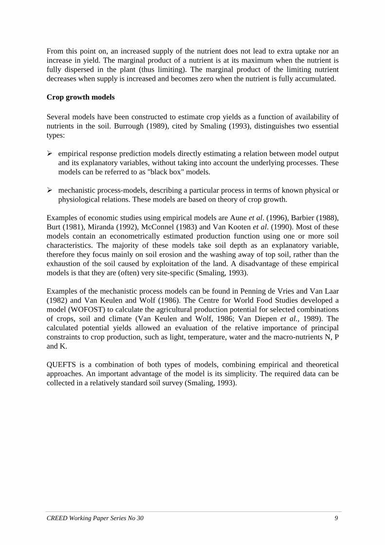
Step 2 Original model In this step the relationship between potential supply (step 1) and actual uptake of the three nutrients (UN, UP, UK) is established. As we have seen above, the plant does not always take up all nutrients; actual uptake is then smaller than the potential supply of a nutrient. In QUEFTS the actual uptake of a nutrient is calculated twice for each nutrient, each time only one of the other two nutrients is taken into account. For instance, the actual uptake of nitrogen (UN) is calculated once as a function of own supply (SN) and the supply of phosphorus (SP) and once as a function of own supply (SN) and the supply of potassium (SK). On theoretical grounds, when we draw the relationship between potential supply and actual uptake, we assume a concave curve (see Figure 4). When a nutrient is no longer absolutely limiting (point 1), a decreasing part of the nutrients is taken up by the plant. Total uptake will increase until the nutrient is maximally accumulated. At that point additional supply will no longer be taken up by the plant.
1
45°
2
A B C
SN
UN
uptake N
supply N
Figure 4 Actual uptake of nitrogen, as a function of the supply of N and a fixed supply of P
In this figure the actual uptake of nitrogen (UN) is depicted against the potential supply of nitrogen, given the supply of the other nutrients. Although the supply of eg, phosphorus is fixed, the uptake of phosphorus varies with the supply of nitrogen. When the supply of

CREED Working Paper Series No 30 15
nitrogen is very small compared to the supply of phosphorus, the whole supply of N will be taken up by the plant (part A). In this case actual uptake equals potential supply. When the supply of N is very large, the whole supply of P will be taken up. According to the law of the minimum a further increase of N will not result in additional uptake of N (situation C). In part B of the curve, N moves from a situation of maximum dilution to a situation of maximum accumulation, referring to a change in technical coefficients. In QUEFTS the relation between the potential supply of a nutrient and the uptake of that nutrient is assumed to be a parabolic one, assuming a linear decrease of dU/dS from 1 in point 1 to 0 in point 2. In field trials controlling for the supply of nutrients, and after analysis of nutrient contents in the plants, the relationships between actual uptake and yield could be estimated in the case of maximum dilution and maximum accumulation. These two situations can be seen as the outer bounds of the yield- uptake curve. With these empirical relationships the co-ordinates of points 1 and 2 can be found except for SN2. In point 1, N is maximally diluted, which means that equation (13) is valid, implying a yield of 70*(UN-5) could be obtained. At this point phosphorus is maximally accumulated and an increase of nitrogen would lead to dilution of phosphorus and accumulation of nitrogen. In point 1 the maximum yield that could be attained when all the phosphorus would be taken up is Yield=200*(UP-0.4)11. By equating the two yields we can calculate SN1=UN1, given the supply of phosphorus SP.
This means:
SN1=UN1=5+(SP-0.4)(200/70) (9)
We know that in point UN2, nitrogen is maximally accumulated, and phosphorus maximally diluted. In a similar way, using equations (12) and (15) we can calculate:
UN2=5+(SP-0.4)(600/30) (10)
Given the supply of phosphorus, SN1, UN1 and UN2 can be found. With these three values and the assumption that the decrease of dU/dS from 1 in point 1 to 0 in point 2 is linear, the whole curve is fixed and SN2 can be found. For each nutrient two equations are derived, each giving the actual uptake of the nutrient as a function of its own supply (S1) and of one other nutrient (S2) (see Annex 3). U1(2) stands for the actual uptake of nutrient 1, as depending on the supply of nutrient 2. Each equation is made up of three parts, corresponding with the situations A, B and C above. This results in two estimates of actual uptake for each nutrient, for instance UN(P) and UN(K).
In accordance with the law of the minimum, UN equals min[UN(P),UN(K)]. Estimates for the uptake of the two other nutrients, UP and UK, are calculated the same way.
11 However, this amount of phosphorus will not be taken up since uptake only equals supply when the nutrient is
maximally diluted in the plant (see below).

CREED Working Paper Series No 30 16
The supply-uptake relationships as calculated in the original version of step 2 indicate an upper bound of the ‘true’ supply-uptake relationships. At the time the original version of the model was created, no experimental data were available to calibrate this step. Smaling (1993) and Smaling and Janssen (1993) were the first to provide data to do this, which were used in the modified version of the model12. Modified version Step 2 is entirely different under the modified version. According to Smaling, the original model overestimates nutrient uptake for N and K, particularly at low supply values. In the modified version the linear-parabolic-plateau model is replaced by an exponential-plateau model because it better represents the observations at the trials. The exponential model explains the uptake of each nutrient as a function of the supplies of all three. In this model the uptake of an element approaches its supply asymptotically when the supply approaches zero. This is in contrast to the original model where uptake equals supply as long as the nutrient is not maximally diluted. Once the maximum uptake has been realised, the exponential curve changes into a plateau, additional supply does not increase the uptake of the nutrient under consideration. An example of the modified exponential-plateau model for the calculation of UN: If ( )SN SN SK> − × − − −0 5 0 05 0 35 1. ( . / . / ) then UN UN= max
Else: UN SN e SN SP SN SK= × × − × − ×{ . ( . / . / )}0 5 0 05 0 35 (11)
The specification of the model implies that even when the supply of a nutrient is absolutely limiting, which means that it is maximally diluted in the plant, the uptake (and hence the yield) depends on the supply of the other nutrients. Extra supply of the other nutrients does increase uptake of the limiting nutrient, and thus of yield. This is in line with Liebscher’s theory of the optimum, whereas strict application of Liebig’s law of the minimum is more consistent with the original QUEFTS. Step 3 For each nutrient upper and lower bound yields are calculated on the basis of the actual uptake of each nutrient (UN, UP, UK). The upper bound yield refers to the yield attainable when for instance N is maximally diluted in the plant, the Yield N maximally Diluted (YND). The lower bound yield refers to the Yield N maximally Accumulated (YNA), the yield that could be obtained when N is maximally accumulated in the plant. The actual yield will be somewhere in-between these yields (see Figure 5). The yields can be calculated with the following empirical relationships:
YNA = 30*(UN-5) (12) YND = 70*(UN-5) (13) YPA = 200*(UP-0.4) (14) YPD = 600*(UP-0.4) (15)
12 See Smaling (1993) p.219.

CREED Working Paper Series No 30 17
YKA = 30*(UK-2) (16) YKD = 120*(UK-2) (17)
The parameters of these relationships are estimations of the outer bounds of the yield-uptake relationships and are therefore very round numbers, which indicates that the numbers are a rounded estimate.
YNA
YND
uptake N (UN) kg/ha
yield,t/ha
Figure 5 Yield ranges depending on the actual uptake of nitrogen The upper line represents yields with maximum dilution and the lower line those with maximum accumulation. Step 3 is only slightly changed in the modified version. Two of the nine parameters of the yield-uptake relationships were altered to include all yield-uptake ratio’s found in the trials. The modified yield-uptake relationships are:
YND = 80 × (UN-5) (13.a) YPA = 160 × (UN-0.4) (14.a)
Step 4 Finally the yield estimates are calculated in pairs on the basis of the actual uptake of each nutrient (UN, UP, UK) and the yield ranges calculated in step 3 (YNA, YND, YPA, YPD, YKA, YKD). This will result in six paired estimations (YNP, YNK, YPN, YPK, YKN, YKP), which are averaged. Nutrient bound yields are first calculated in pairs. An estimation of the N bound yield can be given compared to another nutrient, say P. This is done in the following way (see Figure ). For N the upper and lower bound yields (YNA, YND) as a function of the actual uptake of N are given by the empirical equations (12) and (13). The P limited yield range (YPA, YPD), calculated in step 3 are also drawn in the figure. The combined yield estimate must be somewhere between or on the lines drawn in the figure.

CREED Working Paper Series No 30 18
On line YND, N is maximally diluted, which means that N is absolutely limiting. Adding more P would not increase the yield, that means that P is maximally accumulated, which corresponds to the line YPA. When N is maximally diluted, point 3 is the only valid point in the curve.
3
4
YPA
YPD
YND
YNA
YNPcombined yield
for N and P
uptake N (UN)
yield
Figure 6. Calculation of the combined yield estimate for N compared to P (YNP)
The opposite is true for point 4. As a result the combined yield curve must go through point 3 and 4. Fertiliser trials suggest that the uptake-yield relationship between these points is concave. Janssen et al. assume that the shape of this curve is a parabolic one, which has its maximum at point 4. The parabola can be represented in the following way:
( ) ( ) ( )YNP YPA b UN UN c UN UN− = − − −3 3 2 (18)
Where UN3 is the uptake of N in point 3. The unknown parameters of this function can be found when the positions of points 3 and 4 are known, which are known from the empirical relationships of step 3. This results in the following parabola (19):
YNP YPA YPD YPA UN YPAYPD YPA
YPD YPA UN YPAYPD YPA
= + − − −−
− − − −−
2 5 7030 70
5 7030 70
2
2
( )( / )( / / )
( )( / )( / / )
(19)
For the other pairs of nutrients a yield can be calculated in a similar way. In all six calculations an important condition must be fulfilled. A yield calculated for any combination of two nutrients may not exceed the upper limit of the yield range of the third nutrient (in this

CREED Working Paper Series No 30 19
case YKD) or the maximum yield (Ymax). To avoid this, we have to check whether YPD>YKD or YPD>Ymax. If this is the case, YPD in the formula is replaced by the smallest of the three. The maximum yield is 15 tons/ha by default. This maximum can be lowered to adjust for climatic influences like temperature, solar radiation and water supply. Repeating this calculation for all the other nutrient-pairs leaves us with six estimates for the grain yield. The ultimate grain yield is obtained by averaging the six yields. The final yield estimate may sometimes fall below the line of maximum accumulation for one of the nutrients. This indicates that the uptake of this nutrient estimated in step 2 is too high. In the official QUEFTS software, this is corrected by reducing the initial uptake to a maximum value set by imputing the yield estimate in the relationship for maximum uptake (or maximum accumulation) equations 12, 14 or 16. Then step 3 and 4 are repeated, resulting in a corrected yield estimate. This procedure is repeated until the corrected values for uptake and yield are stable13.
Extensions of the model Fertilisation In the formulas above, the natural fertility of a soil is calculated in order to estimate the yield that can be obtained from this land. By adjusting the model it is possible to calculate the yield that can be obtained by adding any amount of fertiliser. Fertilisation influences the potential supply of nutrients, because it adds extra nutrients to the soil. However, not all the nutrients added to the soil in the form of fertilisers can be taken up by plants. Some parts are either unavailable because in the soil they bind to other material, or are lost from the soil by erosion or weathering. The ratio of the amount of a nutrient applied to the soil and the amount that can be taken up by the plant is called the recovery fraction. This fraction of the nutrient recovered by the crop is dependent upon soil, weather, crop properties and husbandry practices (Operations Review Unit, 1995 and Smaling, 1993).
The model can be adjusted in the following way. The extra supply of nutrients generated by the use of fertilisers can be calculated by multiplying the amount of the nutrient applied in kg/ha by the recovery fraction of that nutrient. Values for the different recovery fraction can be found in literature (Van Duivenbooden, 1992). This extra supply of nutrients is simply added to the natural supply of each nutrient calculated above, in order to obtain the total potential supply14. Crops other than maize The model can be extended for other crops. The basic structure of the model remains the same. Step 1 does not change at all, because the calculation of the potential nutrient supply is independent of the crop under consideration. The differences between crops are expressed by different parameters in yield-uptake relation, shown in Figure 5. Each crop has its own parameters in the equations 12-17 and an own yield maximum. In the steps 2 to 4, the
13 This procedure was not presented in the original Janssen et al.(1990) paper but is used in the official QUEFTS
software as well as in our calculations. See also Janssen et al.(1995) p.21. 14 See Janssen and Guiking (1990).

CREED Working Paper Series No 30 20
functional forms of the curves remain unchanged, but the majority of the parameters will change. For most of the important crops grown in the Atacora these parameters are available (see Annex 3), except for yam.
CREED Working Paper Series No 30 21
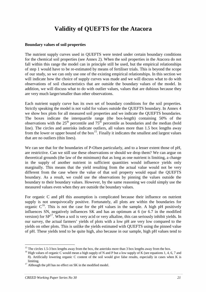
Validity of QUEFTS for the Atacora Boundary values of soil properties The nutrient supply curves used in QUEFTS were tested under certain boundary conditions for the chemical soil properties (see Annex 2). When the soil properties in the Atacora do not fall within this range the model can in principle still be used, but the empirical relationships of step 1 would have to be re-estimated by means of fertiliser trials. This is beyond the scope of our study, so we can only use one of the existing empirical relationships. In this section we will indicate how the choice of supply curves was made and we will discuss what to do with observations of soil characteristics that are outside the boundary values of the model. In addition, we will discuss what to do with outlier values, values that are dubious because they are very much larger/smaller than other observations. Each nutrient supply curve has its own set of boundary conditions for the soil properties. Strictly speaking the model is not valid for values outside the QUEFTS boundary. In Annex 4 we show box plots for all measured soil properties and we indicate the QUEFTS boundaries. The boxes indicate the interquartile range (the box-length) containing 50% of the observations with the 25th percentile and 75th percentile as boundaries and the median (bold line). The circles and asterisks indicate outliers, all values more than 1.5 box lengths away from the lower or upper bound of the box15. Finally it indicates the smallest and largest values that are no outliers (thin lines). We can see that for the boundaries of P-Olsen particularly, and to a lesser extent those of pH, are restrictive. Can we still use these observations or should we drop them? We can argue on theoretical grounds (the law of the minimum) that as long as one nutrient is limiting, a change in the supply of another nutrient in sufficient quantities would influence yields only marginally. This means that the yield resulting from the actual value would not be very different from the case where the value of that soil property would equal the QUEFTS boundary. As a result, we could use the observations by pinning the values outside the boundary to their boundary values. However, by the same reasoning we could simply use the measured values even when they are outside the boundary values. For organic C and pH this assumption is complicated because their influence on nutrient supply is not unequivocally positive. Fortunately, all plots are within the boundaries for organic C16. This is not the case for the pH values in the sample. A high pH positively influences SN, negatively influences SK and has an optimum at 6 (or 6.7 in the modified version) for SP17. When a soil is very acid or very alkaline, this can seriously inhibit yields. In our survey, the actual farmers’ yields of plots with a low pH are very low compared to the yields on other plots. This is unlike the yields estimated with QUEFTS using the pinned value of pH. These yields tend to be quite high, also because in our sample, high pH values tend to
15 The circles 1.5-3 box lengths away from the box, the asterisks more than 3 box lengths away from the box. 16 High values of organic C would mean a high supply of N and P but a low supply of K (see equations 1, 4, 6, 7 and
8). Artificially lowering organic C content of the soil would give false results, especially in cases when K is limiting.
17 Although the pH has no effect on SK in the modified model.

CREED Working Paper Series No 30 22
come together with a high P-Olsen18. QUEFTS results are very sensitive to changes in pH, especially at high pH and low exch.K. When the pH is manually lowered by pinning it, this may lead to a significant overestimation of the yield. Because the effects of pH on yields are so complex, it is not clear whether pinning is acceptable. We therefore chose to discard observations with a pH outside their boundary value. This choice does not have serious implications for the analysis because only few plots have a pH outside their boundary values. Because we have to use the supply curve of the original model for SN, we have to discard all observations with a pH outside the 4.5-7.0 interval. This concerns only 23 observations, and another 5 when we also use supply curves from the modified model (boundaries 4.7-8.0). This automatically removes the values of P-total that are outside the QUEFTS boundary because they come together with a high pH and are also removed from the sample in the same way.
So far we have assumed soil characteristics measurements have been carried out correctly. However, many of the values that are outside the boundary values for QUEFTS are very large/small compared to the other observations. These values are questionable in the sense that they can be the result of a measurement error. This brings us to the problem of outliers - which is not the same as a value outside the QUEFTS boundary. In the search for outliers we want to detect dubious values in the sense that they are the result of an error. Errors are not necessarily made at the upper or lower ends of the distribution, but in these cases they often have a much larger influence on the results. There are several statistical ways to define outliers. In the box plots of the soil properties in Annex 4 outliers are defined in a non-parametric way, all values more than 1.5 box lengths away from the upper or the lower bound of the box.
However, in step 1, we have seen that many of the soil properties should be related to each other. Organic C should be related to organic N, P-Olsen to P-total, Organic C to P-total and pH to exch K. In Annex 5 we have drawn scatter plots between various soil properties to check whether there are any strange results or outliers. With these scatter plots it should be much easier to detect outliers that are a result of an error. At the same time we can use these plots to reveal how realistic the assumptions are for the Atacora which can help us choose the appropriate nutrient supply curve.
Supply curves and outliers The boundary conditions for the modified version of the model allow for a wider range of soils, including more alkaline soils (higher pH) (Smaling, 1993). In the Atacora soils are found with a pH of between 7 and 8, which makes Smaling’s version of step 1 seem more appropriate than the original version. Unfortunately, we do not have the necessary data to calculate SN for the Smaling version. For calculating SN in step 1, we are forced to use the supply curves from the original model, which are tested only for soils with a pH in the range of 4.5-7.0. This still leaves us the choice between two formulae for the supply of N. In equation (1) the C/N ratio is set at 10. We have drawn the C/N=10 line in the scatter diagram and we see that most plots have a higher C/N ratio, which makes equation (2) more reliable. Six observations have a C/N ratio that is far below 10 and the ratio of the others. Besides that, they have a value of org.N that is very large compared to the average. These 18 The reverse is not true.

CREED Working Paper Series No 30 23
values are suspicious and the observations are discarded from the sample19. When these observations are discarded there are no other values of org.N that are outside the QUEFTS boundaries. In equation (4) org.C is used instead of total P because the latter is usually not determined. However, in our survey total P was determined and therefore there is no reason to use equation (4) instead of equation (5). Moreover, in equation (4) a ratio of P-total/org.C of 25 was used, and from Annex 5 we can see that many observations have a ratio that is much higher. Especially the observations that have very large value for P-total have a ratio of P-total/org.C that is far from 25. Observations with a P-total larger than 1500 mg/kg will be discarded from the survey20. Equation (5) uses P-Olsen as well as P-total, whereas Smaling (1993) concluded that P-Olsen had little explanatory power and used Organic C instead. Comparing equations (4) and (6), we would expect P-Olsen to be related to P-total. In Annex 5 we can see a vague relationship between the two, when we exclude the one very high value for P-Olsen. However, when we focus within the boundary values of QUEFTS (P-total 2000 mg/kg and P-Olsen 30 mg/kg) we see that the relationship has become very weak. Moreover, we see that P-Olsen is very high in general. As much as 55% of the observations are larger than the upper bound for QUEFTS. What should we do with these observations when we use P-Olsen in the supply curve? As argued before, instead of dropping 55% of the observations, we could pin these values to their boundary values or simply use the measured value. This is acceptable when it concerns a very large supply of one of the nutrients. Nevertheless we prefer to use equation (6) from the modified version of the model. This has the advantage that P-Olsen is not used, which appeared to have little explanatory power according to Smaling and which has many values outside the QUEFTS boundaries.
What equation to select for SK is arbitrary. The modified version of SK was tested on different, more alkaline soils. Such soils, with a higher pH, are also present in the Atacora, but are left out as a result of the choice for equation (2) for SN. This makes the choice for equation (8) not self-evident. We have no motive to believe that one specification is better than the other. We have decided to use equation (7). We can detect outliers for Kexch. in Annex 4, where we see there is only one observation that is far off from the other observations. This value, with Kexch larger than 30 mmol/kg, is removed. This coincides with the boundary value for QUEFTS. In this section we have discussed what observations of the soil survey to discard from the analyses in the remainder of the thesis on the basis of relationships between soil properties. The results can be found in Annex 2. In the same way we have decided to use the nutrient supply curves (2), (6) and (7).
19 The observations with org.N>3 g/kg are discarded from the sample. 20 The majority of these observations are discarded anyway because of a high pH.

CREED Working Paper Series No 30 24
QUEFTS Results and Most Limiting Nutrients QUEFTS for different crops As indicated in previous sections, crops differ in their ability to take up nutrients from the soil and, hence, soil fertility is crop specific. QUEFTS was designed to predict maize yields, but we do not want to use QUEFTS for maize only. The original version of the model can be adapted for other crops, by using the parameters that can be found in Annex 3. We do not have parameters for all crops that are important in the Atacora, including yam; instead we calculated QUEFTS yields of another root crop, cassava. We would like to demonstrate the sensitivity of QUEFTS for different crop specifications. If QUEFTS is not very sensitive, we could take QUEFTS for maize as an indicator for soil fertility for all crops in the Atacora. QUEFTS yields were calculated for maize, sorghum, millet, cassava, cowpea and groundnut, with the soil characteristics found in our soil survey, using only those plots that satisfied the boundary conditions. For each crop a climate constrained yield maximum was used (see Table 1). This potential yield was calculated with the FAO Agricultural Planning Toolkit (APT) for the central zone of the Atacora, taking into account solar radiation, temperature, rainfall and evapotranspiration on the basis of monthly average climate data from the climate station in Natitingou. The methodology was applied as in Voortman et al. (1998). For each crop we calculated the correlation between the QUEFTS yields and maize (see Table 1). These correlation coefficients are very high, especially for the cereals. Cowpea and groundnut have a lower correlation with maize yields.
Table 1 Correlation of QUEFTS maize yields with other QUEFTS yields
Correlation coef. with QUEFTS yield maize
yield maximum used
Maize - 6,737 Sorghum 0.986 4,812 Millet 0.990 3,891 Cassava 0.922 / 0.869 4,253 / 3,216 * Cowpea 0.870 3,242 Groundnut 0.856 3,242
Notes: Calculated with the original version of QUEFTS, using parameters of Annex 3. For step 1 equations 1, 6 and 7 were used and a climate adjusted yield maximum for all crops. * Potential cassava yield for the 1995 and 1994 season. Potential yields vary much per season due to the long cropping cycle of cassava. Taking a different potential yield only has a negligible effect on what nutrients are most limiting.
Source: Soil survey from 1995/1996
Once we have calculated the results we can calculate what nutrient is most limiting. We do this by comparing which nutrient has the highest uptake/supply ratio. As we can see from Table 2, nitrogen supply from the soil is less limiting for nitrogen-fixing species than for the

CREED Working Paper Series No 30 25
cereals and cassava. As a result, correlation between QUEFTS maize yields and QUEFTS cowpea and groundnut yields are lower, especially for nitrogen deficit soils. However, even for cowpea and groundnut the correlation with maize yields is high. For the cereals and cassava nitrogen is most often the limiting nutrient, followed by potassium. Although for maize in these calculations phosphorus is slightly more limiting than potassium. We can conclude that QUEFTS is not so much crop specific, but more soil specific, giving a chemical fertility bound potential of a soil. This means that we can use QUEFTS-maize values as a proxy of soil fertility for all crops. By using QUEFTS we have aggregated several dimensions of chemical soil fertility into one single indicator of soil fertility, giving one useful measure of soil fertility incorporating the effects of three macro-nutrients together. Nitrogen is the most limiting nutrient in the sample, except for the cultivation of legumes. For legumes potassium is the most limiting nutrient. Phosphorus is usually not limiting.
Table 2 Most limiting nutrient for different crops (row % per nutrient) N P K most second least most second least most second least Maize 80 19 1 10 49 41 10 32 59 Sorghum 70 30 1 7 22 71 24 48 29 Millet 62 38 1 10 22 69 29 41 30 Cassava 57 41 2 9 26 65 34 33 33 Cowpea 17 35 48 20 45 35 63 20 17 Groundnut 21 52 27 12 27 62 67 22 11 Note: Calculated with the original version of QUEFTS, using parameters of Annex 3. For step 1 equations 1, 6
and 7 were used and a climate adjusted yield maximum for all crops. Calculated with the high potential yield of cassava. Wen calculated with the low potential yield of cassava results change by at most one percent point.
Source: Soil survey from 1995/1996
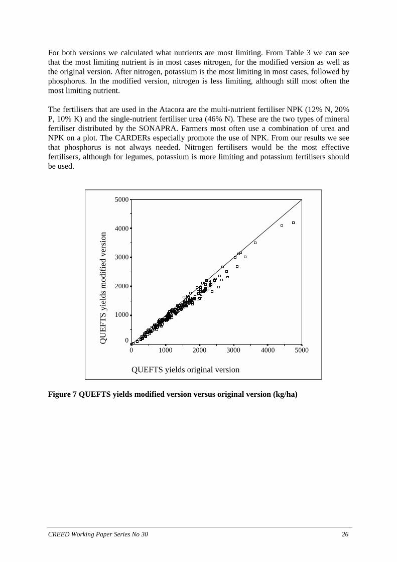
Modified versus original version Since we decided not to use crop specific QUEFTS, which has to be calculated with the original model, the choice between the original or the modified version is still open. Before comparing the two versions of the model, we recalculate the yields with the new yield maximum. Only a very few results alter when the yield maximum is adjusted for climatic factors. When using the original version of the model only 8 yield estimates were altered of the 260. Using the modified version of the model only 6 yield estimates were altered. In all cases the yield estimate was adjusted by less than 1%. This implies that for most of the plots in the sample nutrients are limiting and not the climatic factors like rainfall or temperature. However, there may be other factors limiting production even more, like bad crop management, but this is not taken into account in this yield estimate. Differences in yield in between the modified version and the original version are minor. In a scatter plot of the two versions we see that yields in the modified version are slightly smaller on average, but differences are not large (see Figure 7).
CREED Working Paper Series No 30 26
For both versions we calculated what nutrients are most limiting. From Table 3 we can see that the most limiting nutrient is in most cases nitrogen, for the modified version as well as the original version. After nitrogen, potassium is the most limiting in most cases, followed by phosphorus. In the modified version, nitrogen is less limiting, although still most often the most limiting nutrient. The fertilisers that are used in the Atacora are the multi-nutrient fertiliser NPK (12% N, 20% P, 10% K) and the single-nutrient fertiliser urea (46% N). These are the two types of mineral fertiliser distributed by the SONAPRA. Farmers most often use a combination of urea and NPK on a plot. The CARDERs especially promote the use of NPK. From our results we see that phosphorus is not always needed. Nitrogen fertilisers would be the most effective fertilisers, although for legumes, potassium is more limiting and potassium fertilisers should be used.
QUEFTS yields original version
500040003000200010000
QU
EFTS
yie
lds m
odifi
ed v
ersi
on
5000
4000
3000
2000
1000
0
Figure 7 QUEFTS yields modified version versus original version (kg/ha)

CREED Working Paper Series No 30 27
Table 3 Availability of nutrients in the central zone (number of observations)
Nutrient most limiting
second limiting least limiting partial R2 yield estimate*
original version
SN 223 37 0 .859 SK 27 172 61 .112 SP 10 51 199 .616 modified version
SN 168 71 21 .799 SK 58 54 148 .184 SP 34 135 91 .689 Source: calculations with QUEFTS from Survey VU-UNB 1996 * R2 from regression of calculated supply of each nutrient with ultimate QUEFTS yield. The supply of N (SN) also explains a larger part of the yield estimate than the other nutrients. The reason why the supply of P also explains a large part of the variation in yield is that SP and SN are correlated in our sample (see Table 3). The results of the modified version of the model and the original version of the model are quite similar, although according to the original version Nitrogen is relatively more limiting.

CREED Working Paper Series No 30 28
QUEFTS Results by Village and Land Use Villages In this section we present the results of the QUEFTS-scores for the central zone of the Atacora. We use the modified QUEFTS maize yields as an indicator of soil fertility. In this way we can compare the fertility of soils between villages. These differences in soil fertility can be explained by soil type, differences in fallow periods as a result of differences in pressure on land and perhaps different crop management habits related to ethnic group. QUEFTS may be very site specific, varying from village to village and showing little variation within the village. The box plots in Figure 8 shows us the distribution of QUEFTS yields for each village.
172222202422171818212530N =
Kawado
KanteKagnifele
Bohodo
PouyaKounintchangou
Kounapeikou
Yetapo
TahouPabegou
GaloraPargoute
QU
EFTS
mod
ified
ver
sion
kg/
ha
4500
4000
3500
3000
2500
2000
1500
1000
500
0
Figure 8 Box plot of modified QUEFTS for different villages
The spread between the largest and the smallest value of QUEFTS is 1,500 kg/ha or more for most villages (outliers not included). Even though the spread of QUEFTS varies quite substantially between villages, mean QUEFTS values are not significantly different for most villages. This can be seen from the 95% confidence intervals for QUEFTS values in Figure 9. Apart from the fertile villages Kounintchangou and Kagnifele and the less fertile village Kante, mean QUEFTS values are relatively close together.

CREED Working Paper Series No 30 29
172222202422171818212530N =
Kawado
KanteKagnifele
Bohodo
PouyaKounintchangou
Kounapeikou
Yetapo
TahouPabegou
GaloraPargoute
QU
EFTS
mod
ified
ver
sion
kg/
ha2200
2000
1800
1600
1400
1200
1000
800
600
400
Figure 9 Confidence intervals (95 %) for mean modified QUEFTS values per village We can conclude that although there are differences between villages, these are not much larger than differences within villages. This is important in the analysis because it indicates that village specific factors are less important than individual behaviour of farmers in explaining differences in soil fertility. Cultivation periods and fallow We expect variation in QUEFTS values between plots as a result of the cropping history or the rotation cycle. If this is the case we should see differences in QUEFTS values for plots at different stages in the rotation cycle. Since we have taken soil samples at one point in time only (after the 1995 season), all we can do is make a cross-section of plots and calculate QUEFTS scores for plots at a different stage in the rotation cycle. In Figure 10 the confidence interval of f.i. “2 years” is the 95% confidence interval of mean QUEFTS of all plots that have been cultivated for two seasons (1994 and 1995) since the most recent fallow (1993). We can see a downward trend in QUEFTS value with years of cultivation, although it is not very large. Plots in fallow are the least fertile on average. Is this what we would expect, given that a plot regains soil fertility when under fallow? The explanation may be that the increase in nutrient supply after a fallow partly comes from the ashes of burnt fallow vegetation, which does not show up in soil analysis and as a result not in QUEFTS. Moreover, in our soil survey sample

CREED Working Paper Series No 30 30
we have relatively many observations on plots that have been in fallow only very recently. It is likely that these plots have a very low soil fertility because it is the infertile plots which are put to fallow. As a result the estimation of mean QUEFTS of fallow plots is biased downward. When looking at the QUEFTS value of plots that are used for the first time since they are in fallow (1 year in Figure 10), we can see that their fertility level is higher than the average. This indicates there is a fertility increasing effect of fallow.
1012421202565N =5 and more
4 years
3 years
2 years
1 yearfallow
QU
EFTS
mod
ified
ver
sion
kg/
ha
2000
1800
1600
1400
1200
1000
800
600
Figure 10 QUEFTS score at different years of cultivation Crop choice We expect farmers to take into account soil fertility when choosing what crop to grow on which plot. To be able to see this we compared the QUEFTS yield for maize between plots cultivated with different crops (Figures 11 and 12). The QUEFTS-score used is not crop-specific and is calculated in the same way on all plots. The confidence interval for, eg sorghum is that for those plots on which sorghum was cultivated in the previous season (1995), or sorghum intercropped with another crop. This means that the QUEFTS value of a maize-sorghum intercropping is used twice, once for maize and once for sorghum. QUEFTS results always refer to maize yields, the names of the crops in the figure only indicate the location where the soil samples were taken and the

CREED Working Paper Series No 30 31
mentioned crop was grown. The confidence interval for ‘1st year’ in the figure refers to all plots that are used for the first time since they have been in fallow in 1994. The differences between the crops are not very pronounced. Maize and cowpea are somewhat above the average. Plots in fallow are slightly below the average, whereas first year crops are grown on plots with above average QUEFTS scores. The differences may not be so pronounced because differences in QUEFTS between villages may counterbalance the effect. It is possible that maize is not a crop grown on relatively fertile plots, but is a popular crop in villages that happen to have high QUEFTS scores.
2565112628414769N =1st year
fallowcowpea
groundnut
maizemillet
yamsorghum
QU
EFTS
mod
ified
ver
sion
kg/
ha
2500
2000
1500
1000
500
Figure 11: Confidence interval (95%) for mean QUEFTS values for different crops

CREED Working Paper Series No 30 32
2565112628414769N =1st year
fallowcowpea
groundnut
maizemillet
yamsorghum
QU
EFTS
in %
dev
iatio
n80
60
40
20
0
-20
-40
Figure 12:Confidence intervals (95%) for QUEFTS values in deviation from village average
(%) To correct for this effect we use deviations from village mean and compare these for the main crops (see Figure 12). The differences between crops are now more pronounced, especially for millet. An exception is the difference between plots in fallow and plots in their first year after fallow, which has become smaller. However, fallow plots still have an average soil fertility below village mean. This difference is significant at the 10% level.
Millet tends to be grown on the least fertile soils. This is not surprising since it is not a very demanding crop and usually grown at the end of the rotation cycle. Maize is a more demanding crop and is generally grown on soils that are more fertile than the village average. The mean QUEFTS of cowpea is similar to that of maize. Cowpea is often intercropped with other crops and is therefore found on a variety of soils. The higher QUEFTS mean for cowpea and maize may be a result of the timing of the measurement. We have to keep in mind that QUEFTS is calculated on the basis of soil characteristics measured after the crop has been harvested. Cowpea fixes nitrogen from the air; it is possible that residues of nitrogen were measured on cowpea plots, resulting in higher QUEFTS scores. However, we would expect a similar result for groundnut which also fixes nitrogen. Maize is sometimes grown with mineral fertiliser, which may affect QUEFTS scores.
It is interesting to see that yam is not necessarily grown on fertile plots. Farmers usually grow yam in the first year(s) of the rotation because it is a demanding crop21. However, the QUEFTS score for yam is not as high as for maize and cowpea. Again, the timing of the measurement could be a contributory factor. Perhaps yam was grown on plots that were more 21 Personal communications with farmers.

CREED Working Paper Series No 30 33
fertile than average before the season but after the crop has been harvested the QUEFTS score is around average. Crucial in this respect is to know how fast QUEFTS can change over one year. Figure 10 suggests that even over a short period of one year a change in QUEFTS is perceptible, although the figure is based on cross-section data.
We can conclude from the QUEFTS results for the central zone of the Atacora that although there are differences between villages, the variation between villages is not much larger than within villages. This means that causes for variation in QUEFTS are not purely site specific and probably cannot be attributed to differences in soil type alone. We can see a clear cycle in QUEFTS values through the rotation cycle. QUEFTS scores also vary with crop choice, although interpretation of the results may be hampered by the timing of the measurement. The soil samples were taken after the harvest period and it is possible that QUEFTS captures the effect of mineral fertiliser and the nitrogen fixing ability of legumes, giving a higher result on maize, groundnut and cowpea plots on average.

CREED Working Paper Series No 30 34
QUEFTS Yields and Farmers’ Yields So far we have only looked at the soil fertility side of production, not at any other inputs. We would like to know how limiting soil fertility is compared to other inputs, in order to assess investments in soil fertility. By comparing QUEFTS yields and actual yields we can examine whether soil fertility is actually limiting. In Table 4 we can see that QUEFTS yields are very large compared to the yields actually obtained in the central zone. This means that factors other than soil fertility must also be limiting.
Table 4 QUEFTS yields compared with actual yields
QUEFTS yield* Actual (pure crops) yield
Observation with QUEFTS and Actual
mean (N=192) mean N QUEFTS Actual N
Maize 1.417 1.002 28 1.471 1.069 14
Sorghum 1.268 775 72 1.267 800 37
Millet 1.180 468 44 1.158 505 20
Cassava 2.473 850 2 - - 0
Cowpea 1.337 464 5 1.439 440 2
Groundnut 1.561 599 55 1.667 695 21 *Over all cultivated plots from the soil survey (N=192) Note: QUEFTS is calculated by using crop specific parameters and a crop specific yield maximum. Source: Survey VU-UNB 1996
This result is strengthened by the partial correlation between farmers’ yields with QUEFTS maize yields for the major pure grown crops. Calculating crop specific QUEFTS yields would not give very different results. The yield level may be different but the correlation will not differ very much because the results we get from QUEFTS calculated with specific crop parameters are all highly correlated. From Table 5 we can see that soil fertility and farmers’ yields are never clearly correlated, with the exception of millet. Again QUEFTS alone is not sufficient to explain actual yields, which means that soil fertility is not the only limiting factor in production. Table 5 Partial correlation between QUEFTS maize yields and farmers' yields
N Original version Modified version
Sorghum 37 0.1041 (0.5397) 0.1716 (0.3099) Yam 24 0.0252 (0.9069) 0.0212 (0.9216) Groundnut 21 -0.0351 (0.8800) 0.0114 (0.9610) Millet 20 0.5189 (0.0190) 0.4700 (0.0365) Maize 14 -0.2163 (0.4577) -0.1417 (0.6290) Note: Probability between parenthesis Source: Survey VU-UNB 1996
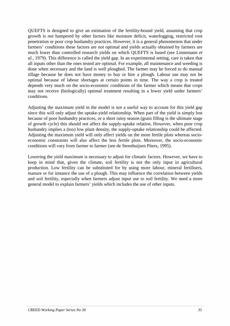
CREED Working Paper Series No 30 35
QUEFTS is designed to give an estimation of the fertility-bound yield, assuming that crop growth is not hampered by other factors like moisture deficit, waterlogging, restricted root penetration or poor crop husbandry practices. However, it is a general phenomenon that under farmers’ conditions these factors are not optimal and yields actually obtained by farmers are much lower than controlled research yields on which QUEFTS is based (see Linnemann et al., 1979). This difference is called the yield gap. In an experimental setting, care is taken that all inputs other than the ones tested are optimal. For example, all maintenance and weeding is done when necessary and the land is well ploughed. The farmer may be forced to do manual tillage because he does not have money to buy or hire a plough. Labour use may not be optimal because of labour shortages at certain points in time. The way a crop is treated depends very much on the socio-economic conditions of the farmer which means that crops may not receive (biologically) optimal treatment resulting in a lower yield under farmers’ conditions. Adjusting the maximum yield in the model is not a useful way to account for this yield gap since this will only adjust the uptake-yield relationship. When part of the yield is simply lost because of poor husbandry practices, or a short rainy season (grain filling is the ultimate stage of growth cycle) this should not affect the supply-uptake relation. However, when poor crop husbandry implies a (too) low plant density, the supply-uptake relationship could be affected. Adjusting the maximum yield will only affect yields on the more fertile plots whereas socio-economic constraints will also affect the less fertile plots. Moreover, the socio-economic conditions will vary from farmer to farmer (see de Steenhuijsen Piters, 1995). Lowering the yield maximum is necessary to adjust for climatic factors. However, we have to keep in mind that, given the climate, soil fertility is not the only input in agricultural production. Low fertility can be substituted for by using more labour, mineral fertilisers, manure or for instance the use of a plough. This may influence the correlation between yields and soil fertility, especially when farmers adjust input use to soil fertility. We need a more general model to explain farmers’ yields which includes the use of other inputs.

CREED Working Paper Series No 30 36
Farmers’ Perceptions of Fertility Asking farmers about the soil fertility of a plot provides a subjective measure and may yield endogenous results in the sense that a farmer will say the soil is fertile when the yields are high. However, taking soil samples incurs enormous costs. In this section we will compare the QUEFTS results based on soil samples with the farmers’ estimation. Where they provide similar results, for certain applications taking soil samples may be omitted to as a budget saving exercise. We asked farmers to estimate fertility of each plot, compared to the average fertility in the village on a scale from 1(low) to 5 (high). The problem with asking the fertility of the plot in general is that it is endogenous, when the yield is bad the farmer will indicate that the fertility is low. Fortunately we asked the farmer this question in the 1995 survey, and it can be seen as a predetermined variable in the 1996 survey. However, there is a timing problem when comparing the farmers’ estimates of fertility to QUEFTS-yields, because the soil samples were taken in the 1996 survey.
In Figure 13 we can see that mean QUEFTS decreases as farmers perceive their plot to be more fertile. For the modified version of QUEFTS in Figure 14 the pattern is slightly more curved but the result is not different.
Whereas QUEFTS is an absolute measure of fertility, the farmers’ estimates are relative to the village average. Looking at the same confidence intervals for QUEFTS in deviation of village mean, the results are less clear, but QUEFTS is certainly not increasing with perceived fertility (see Figure 15). The same result can be seen when looking at the correlation between QUEFTS and fertility as indicated by the farmer. Comparing the correlation between QUEFTS and farmers’ estimates of fertility shows that they are negatively correlated but never significant (see Table 6). However, the negative sign is peculiar.
Regression analysis of the same variables, now adding variables for the 1995 season that could have influenced soil fertility eg, production, crop choice, fertilisation technique etc, did not improve the results, nor change the sign.

CREED Working Paper Series No 30 37
563134486N =
Farmers' estimates of fertility
very highhighaveragelowvery low
QU
EFTS
orig
inal
ver
sion
2000
1800
1600
1400
1200
1000
800
600
400
Figure 13 Confidence intervals of mean QUEFTS (original version) by farmers' estimation of
fertility
563134486N =
Farmers' estimates of fertility
very highhighaveragelowvery low
QU
EFTS
mod
ified
ver
sion
1600
1400
1200
1000
800
600
400
Figure 14 Confidence intervals of mean QUEFTS (modified version) by farmers' estimation of
fertility

CREED Working Paper Series No 30 38
Farmers' estimates of fertility
very highhighaveragelowvery low
QU
EFTS
kg/
ha40
20
0
-20
-40
-60
Original
Modified
Figure 15 Confidence intervals of mean QUEFTS (in % deviation of village average) by
farmers' estimation of fertility
Table 6 Partial correlation of farmers' estimations of fertility and QUEFTS Partial correlation with
fertility Probability
QUEFTS-original -0.0884 0.1576 in difference from village mean -0.0494 0.4303 in % deviation from village mean -0.0587 0.3482 in difference from hh. Mean -0.0304 0.6275 in % deviation from hh mean -0.0343 0.5846
QUEFTS-modified -0.0835 0.1823 in difference from village mean -0.0471 0.4520 in % deviation from village mean -0.0546 0.3832 in difference from hh mean -0.0137 0.8266 in % deviation from hh mean -0.0171 0.7849
Source: Survey VU-UNB 1996
Although the measures do not have to be wrong, they do measure a different concept. There are several soil characteristics a farmer takes into account when evaluating a soil. Perhaps we should have asked more clearly for nutrient content when we asking for an indication of soil

CREED Working Paper Series No 30 39
fertility. A study by Swoboda and Sturm(1995) shows that the soil properties taken into account, as well as the value attributed to each soil property, differ with ethnic group. They studied the soil properties that are considered important by Berba and Peulh farmers in the Pehunco district in the Atacora (see Figure 1). In their study they asked the farmers to map out their soil classifications as well as the soil properties they take into account when evaluating the soil. The results were compared for the two groups. As can be expected, nutrient content was only one soil property considered in evaluating the soil. Others included water content, soil depth, consistency, pebblyness, drainage and workability. Not all farmers agreed on what soil properties were important for a good soil. The research showed that whereas Berba think soil nutrient content, consistency, soil water regime and depth of the soil are important qualities, the Peulh consider workability as the most important soil quality. In the Pehunco research area, the traditional land access rights are with the Berba. According to the authors the Peulh only have access to marginal soils with low nutrient content. Nutrient content is therefore not an important criterion for selection of a soil. The use of manure enables the Peulh to compensate for the low nutrient content. We can conclude that QUEFTS gives very different results of soil fertility than those given by the farmers themselves. This may be due to the different timing of the measurement. We do not know exactly what each farmer takes into account when estimating fertility, but it is likely to comprise more than just nutrient content. The meaning is likely to vary with ethnic group. Although asking farmers in more detail about soil properties seems to be a promising alternative, soil sampling does not seem to be superfluous as yet.

CREED Working Paper Series No 30 40
Conclusions
The purpose of this paper was to determine and discuss a measure of soil fertility, particularly whether an objective measure based on soil sampling is necessary or whether farmers opinions are sufficient.
After a short description of the sources and roles of soil nutrients we introduced a measure of soil fertility: QUEFTS (QUantitative Evaluation of the Fertility of Tropical Soils). To obtain values of the soil properties needed to calculate QUEFTS, soil sampling was undertaken for 295 plots in the centre zone of the Atacora. An extensive description of the model was provided. QUEFTS gives an estimate of potential yields, taking into account the availability of the three macro-nutrients: Nitrogen (N), Phosphorus (P) and Potassium (K). The model was designed for the quantitative prediction of maize yields on unfertilised tropical soils, but it can be adjusted for other crops and fertilisation. Two major versions of the model exist that are referred to as the original version and the modified version. QUEFTS is valid under certain boundary conditions for these soil properties. For most soil properties the boundaries were not very restrictive, except for P-Olsen. To find the true outliers of the soil properties in the soil survey, we inspected proportions between two soil properties. Many soil properties are related to each other and in this way outliers or errors can be easily found.
Using the results of the soil samples of the centre zone, QUEFTS turned out not to be very crop specific but more soil specific. We decided to use the modified model for QUEFTS maize yields as a proxy for soil fertility for all crops. In QUEFTS we have aggregated several dimensions of chemical soil fertility into one single indicator of soil fertility, incorporating the effects of the three macro-nutrients together.
The results of QUEFTS for the soil samples show that Nitrogen is the most limiting nutrient in the sample zone. Phosphorus is in quite ample supply and is usually not yield limiting. Potassium is usually not yield limiting, but it could be in some cases especially for legumes. Nitrogen fertilisers are most effective in the sample area and policy focusing on increasing productivity should enhance the distribution of nitrogen fertilisers.
When we compare QUEFTS results we see large differences within villages and across villages. However, differences across villages are not much larger than differences within villages. This means that QUEFTS measures micro-level differences in soil fertility and not only village or regional differences.
QUEFTS yields show a decline with the number of years a plot is in cultivation. Plots in fallow show low QUEFTS yields. The fertility increasing effect of fallow vegetation which is released when the plot is cultivated cannot be measured by QUEFTS as long as the plot is still in fallow. QUEFTS also varies with the crop grown. As we would expect, maize is grown on the more fertile plots and millet on the less fertile plots. Unlike we would expect, yam does not seem to be grown on more fertile plots. This result may be due to the timing of the measurement of soil fertility. Samples were taken after the season and fertility may have dropped already as yam is a demanding crop.

CREED Working Paper Series No 30 41
When we compare QUEFTS yields to actual yields obtained by farmers, QUEFTS yields are much higher and do not correlate with actual yields, except millet. This implies that soil fertility is not the only limiting factor in the central zone of the Atacora. Knowing how limiting soil fertility actually is requires an estimation of a more general model that includes the use of other inputs.
Returning to the farmers’ own opinions about soil fertility we can conclude that QUEFTS seems to measure very different aspects of soil fertility than those which farmers base their opinions on. The farmers’ estimates of fertility is likely to comprise more than nutrient content. A solution for further research may be to ask farmers in more detail about soil properties. However, as yet we have no reason to say that for economic applications like production function estimation, soil sampling is redundant.

CREED Working Paper Series No 30 42
References Aune, J., Glomsrød, S., Iversen, V. and Wiig, H. 1996. The interdependence between soil degradation and economic growth in Tanzania. Agricultural University of Norway. Barbier, E.B. 1988. The economics of farm-level adoption of soil conservation measures in Upland Java. Environment Department Working Paper no. 11. World Bank, Washington DC. Bradshaw, A.D. and Chadwick, M.J. 1980. The restoration of land. Studies in Ecology Vol. 6. Blackwell Scientific Publications, UK. Burrough, P.A. 1989. ‘Matching spatial databases and quantitative models in land resource assessment.’ Soil Use Management 5: 3-8. Burt, O.R. 1981. ‘Farm level economics of soil conservation in the Palouse Area of the Northwest.' American Journal of Agricultural Economics 63: 83-92. Euroconsult (ed). 1989. Agricultural compendium for rural development in the tropics and subtropics 3rd ed.. Elsevier, Amsterdam, Oxford, New York and Tokyo. Fitzpatrick. 1986. An introduction to soil science. 2nd ed.. Longman, Essex, UK. Gibbon, D.P. and Pain, A. 1985. Crops of the drier regions of the tropics. Longman Group, Essex, UK. INSAE.1994. Deuxième recensement général de la population et de l'habitation - février 1992 - la population de l'Atacora. Institut National de la Statistique et de l'Analyse Economique, Cotonou, Benin. Janssen, B.H. and Guiking, F.C.T. 1990. ‘Modelling the response of crops to fertilizers.’ In: M.L. van Beusichem (ed). Plant nutrition - physiology and applications. Developments in plant and soil sciences no. 41. Kluwer Academic Publishers, Dordrecht. Janssen, B.H., Guiking, F.C.T., Van der Eijk, D., Smaling, E.M.A., Wolf, J. and Van Reuler, H. 1990. ‘A system for quantitative evaluation of the fertility of tropical soils QUEFTS.’ Geoderma 46: 299-318. Janssen, B.H., Guiking, F.C.T., Braakhekke, W.G., and Dohme, P.A.E. 1995. Quantitative evaluation of soil fertility and the response to fertilizers. Wageningen Agricultural University, Dept. Soil Science and Plant Nutrition, Wageningen, the Netherlands. Linnemann, H., De Hoogh, J., Keyzer, M.A. and Van Heemst, H.D.J. 1979. MOIRA, Model of International Relations in Agriculture. North-Holland, Amsterdam, New York, Oxford. McConnel, K.E. 1983. ‘An economic model of soil conservation.’ American Journal of Agricultural Economics 65: 83-89. MDR 1993. Compendium des statistiques agricoles et alimentaires 1970-1992. Ministère du Developpement Rural, Cotonou. MDR/DAPS 1995. Document of the round table on the rural sector. Ministère du Developpement Rural, Direction de l’Analyse, de la Prévision et de la Synthèse, Cotonou.

CREED Working Paper Series No 30 43
Miranda, L.M. 1992. ‘Landowner incorporation of onsite soil erosion costs: an application to the conservation reserve program.’ American Journal of Agricultural Economics 74: 434-443. Operations Review Unit, IOV. 1995. Fertiliser aid. evaluation of Netherlands fertiliser aid 1975-1993, with special reference to Bangladesh, Mali and Zambia. Netherlands Development Cooperation, The Hague. Penning de Vries, F.W.T. and Van Laar, H.H. 1982. Simulation of plant growth and crop production. Centre for Agricultural Publishing and Documentation, Wageningen. Smaling, E. 1993. An agro-ecological framework for integrated nutrient management. Wageningen Agricultural University, Wageningen. Smaling, E.M.A. and Janssen, B.H. 1993. ‘Calibration of QUEFTS, a model predicting nutrient uptake and yields from chemical soil fertility indices.’ Geoderma 59: 21-44. de Steenhuijsen Piters, B. 1995. Diversity of fields and farmers: explaining yield variations in Northern Cameroon. Wageningen Agricultural University, Wageningen. Swoboda, J. and Sturm, H.J. 1995. ‘Traditionelle bodennutzingssysteme und bodenbewertung bei ackerbauern und tierhaltern in Nord-Benin.’ Die Erde 126: 53-71. Van Diepen, C.A., Wolf, J., Van Keulen, H. and Rappoldt, C. 1989. ‘WOFOST: a simulation model of crop production.’ Soil Use and Management 5: 16-24. Van Duivenbooden, N. 1992. Sustainability in terms of nutrient elements with special reference to West-Africa. Report no. 160. CABO-DLO, Wageningen. Van Keulen, H. and Wolf, J. 1986. Modelling of agricultural production: weather, soils and crop. Centre for Agricultural Publishing and Documentation, Wageningen. Van Kooten, G.C., Weisensel, W.P. and Chinthammit, D. 1990. ‘Valuing trade-offs between net returns and stewardship practices: the case of soil conservation in Saskatchewan.’ American Journal of Agricultural Economics 721: 104-113. Van der Pol, F. 1992. Soil mining: an unseen contributor to farm income in Southern Mali. Royal Tropical Institute, Amsterdam. Van Reuler, H. and Prins, W.H. (eds). 1993. The role of plant nutrients for sustainable food crop production in sub-Saharan Africa. Vereniging van Kunstmest Producenten, Leidschendam. Voortman, R.L., et al. 1998. Climate change and global agricultural potential; a case study of Nigeria. SOW-VU working paper, SOW-VU/IIASA, Amsterdam/Laxenburg. de Wit, C.T. 1992. ‘Resource use efficiency in agriculture.’ Agricultural Systems 40: 125-151. Wolf, J., de Wit, C.T., Janssen, B.H. and Lathwell, D.J. 1987. ‘Modelling long-term crop response to fertiliser phosphorus: I. The model.’ Agronomy Journal 79: 445-451.

CREED Working Paper Series No 30 44
Annex 1 The Atacora soil survey Analysis of the soil samples was carried out under the responsibility of Dr. N. Mallouhi at the soil science laboratory of the FSA-UNB. The following soil properties were investigated for 295 plots in the centre zone in the Atacora:
- pH(H2O) acidity - org.C organic Carbon - P-Olsen Phosphorus-Olsen - exch. K exchangeable Potassium - org. N organic Nitrogen - total P total Phosphorus
Samples were taken from the 0-20 cm soil layer. The same analytical procedures were followed as in Janssen et al. (1990):
pH: in supernatant liquid of a 1:2,5 soil-water-suspension, shaking time 2 hours org. C: oxidation by K2Cr2O7, correction factor of 1.03 (Kurmies) org. N: digestion with concentrated H2SO4 and salicylic acid P-Olsen: 5 g of soil in 100 ml 0.5 M NaHCO3, pH adjusted to 8.5, shaking time 30
min. Total P: digestion with Fleischmann’s acid, ratio 2.5:20 exch. K: percolation with 1 M NH4-acetate

CREED Working Paper Series No 30 45
Annex 2 Boundary values Table 7 Measurement units and boundary values for step 1 Boundary values QUEFTS Units original version Modified version boundaries used
PH 4.5-7.0 4.7 - 8.0 4.7-7.0 Org. C g/kg ≤ 70 ≤ 70 Org. N g/kg ≤ 7 ≤ 3 P-Olsen mg/kg ≤ 30 - Total-P mg/kg ≤ 2000 ≤ 1500 Exch. K mmol/kg ≤ 30 ≤ 30 Sources: Janssen et al.(1990) Smaling (1993) Table 8 Number of observations outside the boundary values in the soil survey Number of observations outside boundaries
Original version Modified version Our boundaries used
pH(H2O) 23 14 28 Org. C 0 - 0 Org. N 1 - 6 P-Olsen 163 - - total-P 7 - 8 exch. K 1 - 1 Total discarded 163 14 35 Note: The total number of soil samples is 294 Source: Survey VU-UNB ‘95/’96

CREED Working Paper Series No 30 46
Annex 3 Model specifications for QUEFTS 1. The Original QUEFTS Step 1: Calculation of supply of nutrients (SN, SP, SK) SN SN = max[1.7 × (pH – 3) × org.C , 0] or:
SN = max[17 × (pH – 3) × org.N , 0]
SP SP = max[0.35 × (1 – 0.5 × (pH – 6)2)× org.C + 0.5×POlsen,0] preferably: SP = max[0.0014 × (1 – 0.5 × (pH – 6)2)× Ptot + 0.5×POlsen,0]
SK SK pH exch Korg C
= × − × ×+ ×
max ( . . ) .
. .,250 34 0 4
2 0 90
Step 2: Calculation of the uptake of nutrients (UN, UP, UK) Part 1: calculation of (NPUPT, NKUPT, PNUPT, PKUPT, KNUPT, KPUPT) Formulas for the calculation of 12UPT, where 1∈ {N, P, K} and 2 ∈ {N, P, K} and 1≠2: if S1 < r1 + (S2 – r2)(a2 / d1) then UPT12 = S1 if S1 < r1 + (S2 – r2)(2 × d2 / a1 – a2 / d1) then UPT12 = r1 + (S2 – r2)(d2 / a1)
else: UPT S S r S r a dS r d a a d
12 1 0 25 1 1 2 2 2 12 2 2 1 2 1
2
= − − − −− −
. [ ( )( / )]( )( / / )
Then: 12UPT = max[UPT12,0] The parameters come from the empirical yield-uptake relationships (see step 3 and Table ): Y1A= a1×(U1- r1) and Y1D= d1×(U1- r1) Table 9 Parameters for the original version of QUEFTS Nutrient (1,2) a D r
N 30 70 5 P 200 600 0.4 K 30 120 2

CREED Working Paper Series No 30 47
Example: calculation of NPUPT: if SN < 5 + (SP - 0.4)(200/70) then UPTNP=SN if SN > 5 + (SP - 0.4)(2×600/30 - 200/70) then UPTNP= 5 + (SP - 0.4)(600/30)
else: UPTNP= SN - 0 25 5 0 4 200 700 4 600 30 200 70
2. [ ( . )( / )]( . )( / / )
SN SPSP
− − −− −
NPUPT=max[UPTNP, 0] Part 2: calculation of (UN, UP, UK)
UN= min [NPUPT(SN, SP), NKUPT(SN, SK)]
UP= min [PNUPT(SP, SN), PKUPT(SP, SK)]
UK= min [KNUPT(SK, SN), KPUPT(SK, SP)]
Step 3: Calculation of the yield ranges (YNA, YND, YPA, YPD, YKA, YKD). YNA = 30 × max[0, UN-5] YND = 70 × max[0, UN-5] YPA = 200 × max[0, UP-0.4] YPD = 600 × max[0, UP-0.4] YKA = 30 × max[0, UK-2] YKD = 120 × max[0, UK-2] Step 4: Calculation of the ultimate yield Part 1: Calculation of (YNP, YNK, YPN, YPK, YKN, YKP) Formulas for the calculation of Y12, where 1∈ {N, P, K} and 2 ∈ {N, P, K} and 1≠2: If Y1D>Y2A and Y1A< min[Y1D, Y2D, Y3D, Ymax] and Y2A>MIN then Y12=MIN: If Y1D>Y2A and Y1A< min[Y1D, Y2D, Y3D, Ymax] and Y2A<MIN then:
Y Y A MIN Y A U r Y A dMIN a Y A d
MIN Y A U r Y A dMIN a Y A d
12 2 2 2 1 1 2 11 2 1
2 1 1 2 11 2 1
2
2= + − − −−
− − − −−
( )( / )( / / )
( )( / )( / / )

CREED Working Paper Series No 30 48
Else: Y12= min[Y1D, Y2D, Y3D, Ymax] Where the parameters (r1, d1 and a1) are the same as in step 2, and: MIN = min[Y2D, Y3D, Ymax] Example for YNP:
YNP YPA MIN YPA UN YPAMIN YPA
MIN YPA UN YPAMIN YPA
= + − − −−
− − − −−
2 5 7030 70
5 7030 70
2
2
( )( / )( / / )
( )( / )( / / )
Where
: MIN YPD YKD Y= min[ , , max] Part 2: Calculation of the yield
YE YNP YNK YPN YPK YKN YKP= + + + + +6
Ultimate yield estimate22: YIELD = min[YE, YND, YPD, YKD, Ymax] When YE is smaller then YNA, YPA or YKA then the uptake in step 2 is corrected by using for the over-estimated uptake: Corrected Uptake = (YE/a) + r Where a and r refer to the corresponding parameters of step 2 and 3 (see Table 7 of this Annex). Step 3 and 4 are repeated in the same way until the corrected values for uptake and yield are stable.
Crop specific parameters These are the parameters of the yield-uptake relationships (step 3). Where the parameters in the first row refer to (X = (N, P, K)):
YXA = aX*(UX-rX) YXD = dX*(UX-rX)
22 Boundary condition: harvest index is approximately 0.4; if harvest index > 0.45, YE must be multiplied by
0.5/0.4.

CREED Working Paper Series No 30 49
Table 10 Crop specific parameters used in QUEFTS
RN rP rK aN aP aK dN dP dK Maize 2.7 0.5 4.0 75 29 486 96 150 39 Sorghum 1.3 0.2 2.8 68 20 483 105 84 21 Millet 1.1 0.2 2.8 67 21 465 83 73 19 Cassava 0 0 0 137 50 748 179 126 40 Cowpea 0 0 0 98 48 299 89 45 17 Groundnut 0 0 0 105 58 408 139 52 18 Source: J. Wolf (unpublished)
2. The modified version Step 1: Calculation of supply of nutrients (SN, SP, SK)
SN org Nclay
T
= × ××
−
max .log( %)
,( )/
45 215
09 9
SP = max[(0.0375 × totalP + 0.45 × org.C) × (1 – 0.25 ×(pH – 6.7)2), 0] SK = max[0.35 × (2 + exch.K) × (55 – org.C), 0]
Step 2: Calculation of the uptake of nutrients (UN, UP, UK) Formulas for the calculation of U1, where 1∈ {N, P, K} : if S2=0 or S3=0 then U1=0 if S2>0 and S3>0 and S1 > (–0.5 ×(c1 / S2 + c2 / S3))–1 then U1 = U1max
where: U ec S c S
105 1 2 2 3
1
max . ( / / )= −
× +
−
if S2>0 and S3>0 and S1 < (–0.5 ×(c1 / S2 + c2 / S3))–1 then:
( )U S e c S S c S S1 1 05 1 1 2 2 1 3= × × × + ×. ( / / )
using the following parameters:

CREED Working Paper Series No 30 50
Table 11 Parameters of the Modified Version of QUEFTS
N P K c1 c2 1 2 3 -0.05 -0.35 2 1 3 -1.15 -0.40 2 3 1 -0.35 -0.07
Example: calculation of UN: if ( )SN SN SK> − × − − −05 0 05 0 35 1. ( . / . / ) then UN UN= max
else: UN SN e SN SP SN SK= × × − × − ×{ . ( . / . / )}0 5 0 05 0 35 Step 3: Calculation of the yield ranges (YNA, YND, YPA, YPD, YKA, YKD) YNA = 30 × max[0, UN-5] YND = 80 × max[0, UN-5] YPA = 160 × max[0, UP-0.4] YPD = 600 × max[0, UP-0.4] YKA = 30 × max[0, UK-2] YKD = 120 × max[0, UK-2] Step 4: Calculation of the ultimate yield Step 4 was not modified, the same relationships were taken as under step 4 of the original version, except the modified parameters of step 2 are taken.

CREED Working Paper Series No 30 51
Annex 4 Results of the Soil Survey This Annex shows box plots for all measured soil properties. The boxes indicate the interquartile range (the box-length) containing 50% of the observations with the 25th percentile and 75th percentile as boundaries and the median (bold line). The circles and asterisks indicate outliers, all values more than 1.5 box lengths away from the lower or upper bound of the box. The circles are 1.5-3 box lengths away from the box, the asterisks are more than 3 box lengths away from the box. Finally it indicates the smallest and largest values that are no outliers (thin, short lines). Apart from the box plots we indicate the QUEFTS boundaries, dashed lines are boundaries of the original version and uninterrupted lines are the boundaries of the modified version.
pH Acidity
9
8
7
6
5
4
3
Organic Carbon g/kg
30
20
10
0

CREED Working Paper Series No 30 52
Organic Nitrogen g/k
11
10
9
8
7
6
5
4
3
2
10
P-Olsen mg/kg
500
400
300
200
100
0

CREED Working Paper Series No 30 53
P-total mg/kg
4500
4000
3500
3000
2500
2000
1500
1000
5000
Kexch. mmol/kg
40
30
20
10
0

CREED Working Paper Series No 30 54
Annex 5 Soil properties related Many of the soil properties should be related to each other. Organic C should be related to organic N, P-Olsen to P-total, Organic C to P-total and pH to exch K. This annex shows scatter plots between various soil properties. With these scatter plots it should be much easier to detect outliers that are a result of an error. At the same time we can use these plots to select the appropriate nutrient supply curve.
Organic Nitrogen g/kg
121086420
Org
anic
Car
bon
g/kg
30
20
10
0

CREED Working Paper Series No 30 55
P-total mg/kg
450040003500300025002000150010005000
Org
anic
Car
bon
g/kg
30
20
10
0
P-total mg/kg
450040003500300025002000150010005000
P-O
lsen
mg/
kg
500
400
300
200
100
0
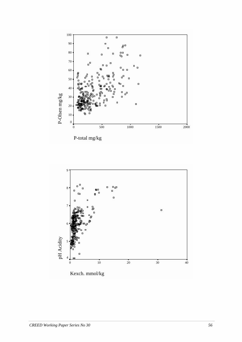
CREED Working Paper Series No 30 56
P-total mg/kg
2000150010005000
P-O
lsen
mg/
kg
100
90
80
70
60
50
40
30
20
10
0
Kexch. mmol/kg
403020100
pH A
cidi
ty
9
8
7
6
5
4

CREED Working Paper Series No 30 57
PUBLICATIONS AND ORDER FORM
Paper Nos. 1-16 may be obtained free of charge; however orders for large quantities (more than 6) will incur postal charges. Full copies of papers Nos. 17 onwards may be downloaded from the CREED web site free of charge, at http://www.iied.org/creed. Alternatively hard copies may be obtained from IIED; a charge of £5 plus postage, will be levied for northern readers only.
The following papers are available from the CREED Programme. Please check the publications you wish to obtain and return the order form to Jacqueline Saunders, Environmental Economics Programme, International Institute for Environment and Development, 3 Endsleigh Street, London WC1H 0DD, or email your requests to [email protected].
CREED Working Paper Series.
# No 1. Adjustment Policies and the Environment: A Critical Review of the Literature. Carlos E.F. Young and Joshua Bishop. July 1995.
# No 2. Environmental Regulations as Trade Barriers for Developing Countries: Eco-labelling and
the Dutch Cut Flower Industry. Harmen Verbruggen, Onno Kuik & Martijn Bennis. July 1995.
# No 3. Economic Incentives for Watershed Protection: A Report on an Ongoing Study of Arenal, Costa Rica. Bruce Aylward, Jaime Echeverría & Edward B. Barbier. September 1995.
# No 4. Economic Policies for Sustainable Water Use in Thailand. Ritu Kumar and Carlos Young. June
1996.
# No 5. The Informal Sector and Waste Paper Recovery in Bombay. Pieter van Beukering, Edwin Schoon and Ajit Mani. June 1996.
# No 6. Economic Trends in the Timber Industry of the Brazilian Amazon: Evidence from
Paragominas. Steven Stone. July 1996.
# No 7. Input Substitution in the Indian Paper Industry: A Variable Cost Function Approach. K.V. Ramaswamy, R.R. Vaidya, M.J. Bennis and J.G.M. Hoogeveen. July 1996.
# No 8. Poverty and Environmental Degradation: A Literature Review and Analysis. Anantha K.
Duraiappah. October 1996.
# No 9. Valuation and Evaluation of Management Alternatives for the Pagbilao Mangrove Forest. Ron Janssen and Jose E Padilla. October 1996.
# No 10. The Economic and Environmental Impacts of the Waste Paper Trade and Recycling in
India: A Material Balance Approach. Pieter van Beukering and Anantha K. Duraiappah. November 1996.
# No 11. Incentives for Eco-efficiency: Lessons from an Evaluation of Policy Alternatives; A Case
Study of the Steel Sector in India. Ritu Kumar, Nick Robins, A.K. Chaturvedi, R. Srinivasan and J. Gupta. December 1996.
# No 12. Poverty and Environment Linkages in Mountains and Uplands: Reflections on the ‘Poverty
Trap’ Thesis. Sanjeev Prakash. February 1997.
# No 13. The Economic Importance of Wild Resources in the Hadejia-Nguru Wetlands, Nigeria. Derek Eaton and Marie-Thérèse Sarch. May 1997.

CREED Working Paper Series No 30 58
# No 14. Economic Valuation of Mangrove Ecosystems: Potential and Limitations. Frank Spaninks and Pieter van Beukering. July 1997.
# No 15. The Use of Environmental Functions to Evaluate Management Strategies for the Pagbilao
Mangrove Forest. Alison J. Gilbert and Ron Janssen. August 1997. # No 16 Trends and Issues in the Plastics Cycle in China, with Special Emphasis on Trade &
Recycling. Pieter van Beukering, Li Yongjiang, Zhao Yumin & Zhou Xin. December 1997. # No 17. Economic Valuation of Communal Rangelands in Botswana: A Case Study. Jaap Arntzen.
February 1998.
# No 18. Environmental Product Measures: Barriers for South-North Trade? Harmen Verbruggen, Onno Kuik, Martijn Bennis, Hans Hoogeveen, Roland Mollerus. March 1998
# No 19. The Shrimp Aquaculture Sector in Thailand: A Review of Economic, Environmental and
Trade Issues. Direk Patmasiriwat, Onno Kuik and Sunil Pednekar. October 1998.
# No 20. An Analysis of Private and Social Discount Rates in Costa Rica. Bruce Aylward and Ina Porras. December 1998.
# No 21. Institutional Arrangements for Watershed Management: A Case Study of Arenal Costa
Rica. Bruce Aylward and Alvaro Fernandez Gonzalez. December 1998. # No 22. Farmers’ Perceptions and Sustainable Land Use in the Atacora, Benin. A. Adegbidi, K.
Burger, E. Gandonou and I. Mulder. February 1999. # No 23. Sustainable Livestock Management in the Kalahari: an Optimal Livestock Rangeland
Model. Anantha K. Duraiappah and Jeremy S. Perkins. March 1999. # No 24. Analysing Urban Solid Waste in Developing Countries: A Perspective on Bangalore, India.
Pieter van Beukering, Madhushree Sekher, Reyer Gerlagh and Vijay Kumar. March 1999. # No 25. Market and Policy Incentives for Livestock Production and Watershed Protection in
Arenal, Costa Rica. Bruce Aylward, Jaime Echeverría, Katherine Allen, Ronald Mejías and Ina T. Porras. March 1999.
# No 26. Integrated Modelling of Solid Waste in India. Reyer Gerlagh, Pieter van Beukering, Madhu
Verma, P.P. Yadav and Preety Pandey. March 1999. # No 27. The Plastics Sector in China: Issues in Production, Recycling and International Trade.
Anantha K. Duraiappah, Zhou Xin and Pieter van Beukering. March 1999.
# No 28. Farmers’ Perceptions of Soil Fertility in Benin Ingrid Mulder. February 2000. # No 29. Automobile Pollution Control in Brazil. Claudio Ferraz and Ronaldo Seroa da Motta.
June 2000.
# No 30. Soil Fertility: QUEFTS and Farmers’ Perceptions. Ingrid Mulder. July 2000.

CREED Working Paper Series No 30 59
CREED Final Reports
The following reports are available from recently completed CREED projects. A charge is levied for all readers as indicated.
# International Trade and Recycling in Developing Countries: The Case of Waste Paper
Trade in India. P. van Beukering and V. Sharma (eds). November 1996. 155 pages. £20
The importance of international trade in the global economy is expanding, not only for primary products but also for recyclable waste. The main objectives of this study were to determine the economic, social and environmental impacts of international trade of waste paper for recycling purposes in India. The report addresses three main sectors: (i) the world market for waste paper, (ii) the local waste paper market and (iii) the Indian paper industry. It also makes recommendations for policy makers at an international, national and local level: international agreements should distinguish between hazardous and non-hazardous waste; national trade barriers to waste imports should be eliminated; and existing local informal recovery sectors should be favoured over formal Western-style recycling systems.
# Mangroves or Fishponds? Valuation and Evaluation of Alternative Uses of a Mangrove
Forest in the Philippines. Ron Janssen & Jose Padilla. September 1997. 258 pages. £25.
One of the major threats to mangroves in the Philippines is the rapidly increasing aquaculture industry. This study includes a review of valuation methodologies and their application to the case study area of the Pagbilao experimental mangrove forest in the Philippines. Valuations of goods and services and environmental functions of the forest are employed to assess alternative management regimes using both cost-benefit analysis as well as a multi-criteria approach. Much depends on the management objectives: conversion to aquaculture is the most economically efficient management option. However, if equity and sustainability objectives are included, commercial forestry is the preferred alternative.
# Incentives for Eco-Efficiency. Market Based Instruments for Pollution Prevention: A
Case Study of the Steel Sector. Ritu Kumar, Nick Robins, A.K. Chaturvedi, R. Srinivasan and J. Gupta. December 1997. 96 pages. £20.
Mounting pressures on industry to reduce pollution, to remain globally competitive and to meet the requirements of international standards, require fundamental changes in government policy and corporate approaches to environmental management. This report presents the results of an international study assessing the potential for market-based instruments for pollution prevention in the steel sector in India. It recommends a set of policy measures to reduce discharge levels in the most cost effective manner, to induce firms to adopt cleaner technologies and to encourage firms to economise on energy and water resources. In this regard, the importance of achieving coherence with existing policies, building trust among key stakeholders and gradually phasing in market-based instruments is emphasised.
# Economic Incentives for Watershed Protection: A Case Study of Lake Arenal, Costa
Rica. Bruce Aylward, Jaime Echeverria, Alvaro Fernandez Gonzalez, Ina Porras, Katherine Allen, Ronald Mejias. February 1998. 323 pages. £30.
Conventional wisdom holds that cutting down tropical forests for livestock production is not only bad business but bad for the environment. In particular, it is thought that conversion of natural forest to pasture leads to a rise in the sedimentation of waterways and resevoirs, increased risk of flooding and loss of dry season water supply. In the case of Lake Arenal, Costa Rica, this conventional view is stood on its head by research showing that ranching,

CREED Working Paper Series No 30 60
dairy farming and associated downstream hydrological effects represent important positive values to the Costa Rican economy, values that significantly outweigh expected returns from reforestation
# Plastics Recycling in China. An International Life Cycle Approach. Edited by Pieter van
Beukering. April 1999. 148 pages. £20.
Please check the papers you wish to obtain and use this form for delivery, to indicate a change of address, or to be added to the mailing list to receive information about future CREED Working Papers (please tick).
Name ................................................................................................................................................... Organisation .......................................................................................................................................
Address ............................................................................................................................................. ............................................................................................................................................................. I enclose a cheque for *£......................made payable to IIED/I authorise you to debit my credit card for
£.............. My Access/Visa/Mastercard number (please tick as applicable) is:
Expiry date.................................... . Name of cardholder............................................................. Cardholder address............................................................................................................................
* For postage within the UK please add 20%, minimum £1 (first class or equivalent) For postage to Europe please add 25%, minimum £2 (printed matter airmail or equivalent) For postage to the rest of the world, please add 40% (printed matter airmail or equivalent) or 25%
(surface)