Social Media Marketing: How Much Are Influentials Worth? ∗

Zsolt Katona †

March 20, 2013

∗Preliminary version. All comments welcome.†Zsolt Katona is Assistant Professor at the Haas School of Business, UC Berkeley, CA 94720-1900. E-mail:

zskatona@haas.berkeley.edu Tel.: +1-510-643-1426

Social Media Marketing: How Much Are InfluentialsWorth?

Abstract

This paper studies the competition between firms for social media influencers. Firms spend effortto convince influencers in a social network to recommend their products. The results show that thevalue of an influencer depends only on the structure of the influence network and not the level ofcompetition in the product market. Influencers who exclusively cover a high number of consumers aremore valuable to firms than those who mostly cover consumers also covered by other influencers. Thetotal effort expended by firms is completely determined by the in-degree distribution of the network.Firm profits are highest when there are many consumers with a very low in-degree or with veryhigh in-degree. Consumers with an intermediate level of in-degree contribute negatively to profitsand high in-degree consumers increase profits when market competition is not intense. Prices aregenerally lower when consumers are covered by many influencers, however, firms are not always worseoff with lower prices. The nature of consumer response to recommendations makes an importantdifference. When first impressions dominate, firm profits for dense networks are higher, but whenrecommendations have a cumulative influence profits are reduced as the network becomes dense. Anextension models the incentives firms provide to influencers and how these affect influencers’ networkformation behavior. Direct monetary incentives lead to dense networks and consumers covered bymany influencers. Such networks are only beneficial to firms when market competition is not intense.When the market is more competitive, firms are better off providing smaller direct incentives justenough to ensure a sparse coverage of consumers by influencers.

1 Introduction

The emergence of social media is transforming the way firms approach consumers. Nielsen reports1

that 92% of consumers trust product recommendations from people they know, vastly exceeding any

form of advertising or branded communication. Recognizing the power of word-of-mouth, marketers

began to reach out to influential consumers, hoping that customers can convince their peers more

effectively than traditional advertising would.

In order to utilize the value of the vast consumer-to-consumer communication networks facilitated

by social media, companies need to: i) identify influencers, and ii) convince influencers to recommend

their products. There are a number of upcoming service providers offering assistance with the first

task. The most notable example is Klout.com, a site that collects data about consumers from social

networks to estimate their influential power. While the task of assigning individual influence scores

is not easy and frequent adjustments to the methodology are necessary,2 various startups have made

good progress in this direction, some of them being able identify influencers at a very granular level.3

Once marketers have identified influencers the next step is to get them to recommend the mar-

keted product. There are different approaches to convincing influencers, but all of them involve

considerable effort from firms. The activities firms conduct can range from simple communications

that demonstrate the value of the product through offering extra perks to directly paying influencers.

For example, Cathay Pacific offers lounge access to customers (of any airline) that have a high Klout

score.4 Other companies such as online fashion retailers Bonobos and Gilt offer discounts, whereas

Capital One provides increased credit card rewards for customers with high influence scores. Some

of these offers go to the length of giving away products for free.5

It is apparent that companies spend considerable effort trying to identify and win over influencers,

but it is not clear what the value of each influencer is and how this value depends on the influence

network between consumers. This problem is reflected in the widespread and intense discussions

1“Global Trust in Advertising and Brand Messages”, Nielsen, April 20122“Klout, Controversial Influence-Quantifier, Revamps Its Scores”, Businessweek, August 14, 20123“Finding Social Media’s Most Influential Influencers”, Businessweek, October 18, 20124“Free Cathay Pacific Lounge Access at SFO via Klout.. If You Are Cool Enough,” available at

http://thepointsguy.com/2012/05/klout-offers-some-free-cathay-pacific-lounge-access-at-sfo/5“Gilt Gives Discounts to Match Klout Scores”, available at http://allthingsd.com/20120305/gilt-gives-discounts-

to-match-klout-scores/

2

among practitioners about the return on investment in social media marketing efforts.6

The conventional wisdom suggests that consumers who have many peers listening to them are

valuable, but this simple prescription that only considers the reach of each influencer does not

take into account the potential overlap between consumers covered by different influencers. In a

competitive environment, it is crucial to understand how firms should value each influencer depending

on which of their peers these influencers can have an impact on. Another commonly held view is

that the more links and communication there is, the better off marketers who rely on influencers are.

Again, this train of thought ignores the potential for competition and the possibility that influencers

may recommend the competitor’s product.

In order to rigorously study the problem of how much effort to spend on influential consumers in

a competitive environment, we develop an analytical model addressing the following questions:

• How much effort should competing firms spend on each influencer depending on the intensity

of competition?

• What is the role of the network structure? Are highly connected influentials always the most

valuable?

• What is the effect of the influence network on prices, firm profits, and consumer surplus?

• How should firms incentivize influentials? Should they offer direct (monetary) benefits or

should they convince them in other ways?

• How will influentials change their network in response to different incentives?

The main model includes two competing firms who try to win over influencers in a network. Firms

exert effort on each influencer and when they succeed the influencer recommends their product.

Consumers who receive recommendations about only a single product provide a unit margin to the

firm selling that product, whereas those who receive recommendations about both products provide

a lower margin to both firms. The exact margin depends on the intensity of competition and can be

as low as zero in a very competitive environment.

We find that the equilibrium is symmetric where the two firms follow the same strategies, but

the effort levels for each influencer differ based on his or her position in the network. We identify

6“Driving Business Results With Social Media”, - Businessweek, January 21, 2011,

3

the equilibrium effort in the most general fashion: for each influencer in any network. Surprisingly,

the effort levels are independent of the intensity of product market competition between firms. This

follows from the phenomenon that firms value influencers for both offensive and defensive purposes.

On one hand, winning over an influencer makes it possible to convey a message to consumers who

do not otherwise receive recommendations about a product. On the other hand, winning over an

influencer prevents the competing firm from having its product recommended to consumers. The

combination of the two effects makes it equally important to spend effort on influencers in both a

competitive and a non-competitive environment (offense pays off more in the latter, defense in the

former).

The equilibrium effort level for a given influencer is a function of the network structure. In

particular, the value of an influencer to firms highly depends on whether consumers covered by this

influencer are covered by other influencers and if yes, by how many of them. Adding up the effort

levels of one firm for all influencers reveals that the total effort exerted is determined by a very

simple network statistic: the in-degree distribution of the influence network. Consumers with a

small in-degree, those who are influenced by only a few influencers, contribute to effort levels less

than those with a high in-degree. As a consequence, highly connected influencers are valuable, but

only if they cover consumers who are not covered by many other influencers. Firm profits depend

on the network structure in an interesting way as the profit is a U-shaped function of the in-degrees.

Networks where each consumers covered by very few, and those where each consumer is covered

by a large number of influencers are the most profitable, whereas networks where each consumer is

covered by an intermediate number of influencers are the least profitable.

To study how recommendations influence purchase decisions in more detail, we extend the model

to include a more elaborate influence process that allows us to examine consumer consideration and

choice together firms’ pricing decisions. In equilibrium, we find that firms employ mixed pricing

strategies while using effort levels similar to those of the basic model to convince influencers. We

find that prices depend on the network structure in an interesting fashion. Firms charge lower prices

to consumers covered by more influencers. As a result, in sparse networks, where consumers are

typically covered by a few influencers, prices are generally high as firms are able to extract almost all

surplus from consumers who only consider one product. At the other extreme, when consumers are

under the influence of many influencers, prices go down as price competition increases. Surprisingly,

4

these lower prices do not always hurt firms. When first impressions about a product determine

consumers’ product considerations, highly covered consumers can increase firm profits as firms cut

back on their efforts trying to convince influencers. When recommendations have a cumulative effect,

firms spend relatively heavily on winning over influencers even in dense networks, resulting in lower

profits.

Finally, we study how firms should incentivize influencers to form their networks and how con-

sumers react to different incentives. In principal, firms have two different ways of making influencers

recommend their product. We find that when firms use a direct, possibly monetary incentive, influ-

encers establish more links, expanding their network. This can benefit or hurt firms depending on the

level of competition. The main result is counterintuitive: when the product market is competitive

firms should not offer a very high monetary benefit to influencers so as to avoid too much coverage.

When the market is not that competitive, firms should encourage influencers to build their network

with substantial monetary benefits.

The rest of the paper is organized as follows. In the next section, we review the relevant literature,

then, in Section 3 we introduce the model. In Section 4, we derive the equilibrium of the basic model.

Next, in Section 5, we examine the pricing decisions and in Section 6, we study the incentives provided

by firms to influencers and the resulting endogeneous network formation behavior. Finally, in Section

7, we conclude and discuss the practical implications and limitations of our results.

2 Relevant Literature

The importance of word-of-mouth communications in marketing has been long recognized by the

literature, starting with the widely employed product diffusion model of Bass (1969). Most of the

early models concerned aggregate effects, but with the new developments in network analysis and

the availability of network data, academic research recognized the need to understand the role of the

underlying network. For example, Goldenberg et al. (2001) studied the diffusion process on a grid as

a special type of network. First on simple, then on more complex networks the marketing literature

has uncovered several important network properties and their contribution to the diffusion process

(Goldenberg et al. 2009, Katona et al. 2011, Yoganarasimhan 2012), helping to identify influencers

(Tucker 2008, Trusov et al. 2010). At the same time, computer scientist have also addressed the

question of how to seed a network optimally to maximize viral spread (Kempe et al. 2003, Stonedahl

5

et al. 2010).

The role of marketing effort in the diffusion process has been further studied by Mayzlin (2002)

who considered the tradeoff between traditional advertising and firm generated buzz, while a stream

of papers (Van den Bulte and Lilien 2001, Nair et al. 2010, Iyengar and Valente 2011) examined the

effects of marketing effort and social contagion in the drug adoption decisions made by physicians

also considering firms’ marketing activities. Godes and Mayzlin (2009) ran a field experiment to

study how a firm’s agents can affect word-of-mouth communications between consumer and find

that the effectiveness depends on the nature of ties.

Most papers in the area focus on how a monopolist should target a few consumers in a network

to optimize the diffusion of a single product or idea, ignoring competition. A notable exception

considering competition in a direct marketing setting is a paper by Zubcsek and Sarvary (2011) who

study competing firms advertising to a social network. They find that it is important for advertisers

to take into account the existence of the underlying network, especially its density. Despite some

similarities, our paper is different in several aspects. Our primary focus is not on seeding strategies

that seek to find optimal targets that would maximize the spread of a given campaign. Instead,

we analyze how firms should invest to win over influencers in a network in order to capture market

share, somewhat akin to Chen et al. (2009). We also take into account that firms can exert different

amount of effort engaging in a contest for each influencer. This allows us to quantify the value of

each influencer which - as our findings show - depend heavily on the distribution of in-degrees.

A notable paper that also considers competition is by Galeotti and Goyal (2009) who present

a simple competitive extension to their model on how to influence influencers. In contrast to our

model, they do not study how firms target specific influencers, reducing the decision to a single

variable on advertising intensity. Finally, He et al. (2012) consider firm incentives in a competitive

setting to induce connections between customers.

Our paper is also related to the literature on targeting and advertising. Our model includes

the ability of firms to individually target influencers, related to Chen and Iyer (2002), Chen et al.

(2001). Papers such as Iyer et al. (2005), Amaldoss and He (2010) study the strategic effects of

targeting and how firms can avoid intense price competition. Similarly to a large proportion of the

prior literature on informative advertising, our treatment of pricing decisions builds on the widely

adopted formulation by Varian (1980), Narasimhan (1988).

6

3 Model

3.1 The Consumer Influence Network

There are M consumers in the market, N ≤M of which are influencers. We call consumers who can

potentially affect their peers’ product choices influencers.7 We order consumers so that the first N

consumers, that is i = 1, 2, . . . , N , are influencers. Each influencer can potentially influence any of

his or her peers, whom we call influencees.

A key feature of our model is the underlying influence network structure that determines the

influencer-influencee relations. This influence network need not be identical to the underlying network

of social connections, as not all of them result in effective influence between consumers. Furthermore,

we only consider the influence that takes place in the context of the relevant products in our model.

Nevertheless, since influence is likely to take place over social links, hence we think of the influence

network as a narrow product-specific subnetwork of the social network.8

We model the influence network as a random network. Let Iij be the indicator variable showing if

a product recommendation takes place (Iij = 1 if yes, 0 otherwise) between influencer i and influencee

j. When Iij = 1, a unidirectional influence link exists between i and j. We say that influencer i covers

consumer j in this case. We use several subscripts to denote consumers throughout the analyses,

but for clarity we distinguish between influencers (denoted by i, h) and influencees (denoted by j, g)

based on their role.

We take a very general approach to model how the random network is generated, where

wij = Pr(Iij = 1) (1)

measures the expected strength of influence of influencer i on consumer j. We do not specifically

model the nature of influence between consumers, which can take several forms. For example, a very

simple type of influence is when one consumer informs a peer about a product, making him or her

consider it.9 A more complex form of influence is when consumers share positive information about a

product and try to convince their peers about the product benefits. Regardless of the specific process,

7In theory, all consumers could be influencers (and our model allows this), but to paint a more realistic picture, weassume that only a proportion of them has enough influential power to significantly effect others’ choices.

8In Section 6 we consider an extension, where consumers decide on their influence levels over existing social links.9We use this specification in Section 5 when modeling pricing strategies.

7

we assume that a higher wij corresponds to a higher likelihood of an effective correspondence taking

place.

The influence network matrix W is defined as the collection of wij values. We assume that W is

common knowledge, but that the outcome of each random variable is not observed by players. One

can think of W as the adjacency matrix of the weighted network which is obtained as the expected

influence network between consumers. For example, if all wij ∈ {0, 1}, then the influence network

is deterministic and the expected network is the same as the actual influence network. However,

it is more realistic to assume that players do not observe the exact network, especially since this

network is not identical to the underlying social network. Product influence rarely takes place with

high probabilities on all social network links. That is, W represents what firms believe the influence

network could be. With the emergence of social network analytic technologies and services these

beliefs become more and more accurate. Companies like Klout provide measures about consumer

influence levels, and although some of these measures are still rudimentary, there is rapid development

is this area. Our model is very flexible with regards to how much information firms have about the

influence network ranging from one extreme of complete information (represented by a deterministic

W) to the other extreme of a no or little information. Firms in this case would have some prior

belief about how the influence links are distributed, resulting in a stochastic W matrix with large

variances.

An important quantity in our analysis is the total number of influencers that cover a particular

influencee. We call this influencee j’s in-degree and denote it by dj . We also need to count this

quantity separately for consumers covered by a particular influencer. In summary, we introduce the

notations

dj =N∑h=1

Ihj , ϕki =

M∑j=1

Pr (Iij = 1, dj = k) , and ϕk =1

k

N∑i=1

ϕki. (2)

That is, ϕki counts the expected number of consumers covered by i, who are influenced by exactly

k influencers (including i), whereas ϕk measures the expected frequency of consumers covered by k

influencers in the entire network. ϕk can also be interpreted as the expected in-degree distribution of

the influence network, whereas ϕki is the expected degree distribution among consumers covered by

influencer i. Since our setup is very general in terms of the network structure, we derive the solution

for any type of degree distribution. However, in order to ensure an equilibrium in pure strategies,

8

we assume that ϕ1i is not too small for any influencer.10

3.2 Firms and Influencers

We assume that there are two firms (f = 1, 2) selling their products to the M consumers. Firms

take advantage of social media and target influencers to increase the revenue they can expect from

consumers. Consumers thus influence their peers to buy the product of one of these (or both) firms.

Let Rf denote the set of consumers who receive recommendations only about the product of firm

f , whereas R12 the set of those who receive recommendations about both products. In our baseline

model, we assume a simple revenue structure for firms who sell their products at zero variable cost.

Each consumer j ∈ Rf provides a revenue of 1 to firm f , whereas a consumer j ∈ R12 provides a

revenue of q ≥ 0 to both firms. In essence, q measures the intensity of competition between the

two firms. When q = 0, the two firms are competing heavily and cannot extract any profits from

consumers that strongly consider both products. As q increases to 1/2 the competition becomes

less intense and while the products are still substitutes, firms can extract the same amount of profit

from these consumers as from those only considering one product. As q increases further, the two

products eventually become complements.

Although we do not directly model the product market competition in this basic model, there

are several micromodels that produce results corresponding to our assumption. For example, if we

assume that personalized pricing is possible, Bertrand competition leads to q = 0 when consumers in

R12 compare the two products. Higher q values could be obtained using a bargaining or differentiation

models (e.g. in a linear city q would roughly correspond to t/v.) In Section 5, we present such an

extended version of the model, where firms make pricing decisions and show that it can correspond

to our basic model with any 0 ≤ q < 1. In that model, we assume that firms are able to price

discriminate across consumers, but we do not require firms to learn more about consumer identities

that they already know from the influence network. Furthermore, even if personalized pricing is not

possible, and all consumers pay the same price, one can produce similar results.

We assume that the N influencers have a limited bandwidth to talk to their peers and they

only recommend one product. This is consistent with survey results11 showing that influencers

10Formally, we need ϕ1i ≥ C(1/4)∑∞

k=1 ϕki, where C depends on the model parameters, but a C of around 1/4 istypically sufficient. This is a technical assumption which does not put too much restriction on the network structure,especially if the wij probabilities are relatively small.

11“Three Surprising Findings About Brand Advocates”, Zuberance Whitepaper, February 2012, available at

9

recommend a limited number of products, most of them less than ten per year. Since this already

low number of recommendation is split over different product categories, it is plausible to assume that

most influencers recommend only one of two competing products. To become the one recommended

brand, firms invest resources to convince influencers to recommend their product. For each influencer,

let efi denote the effort spent by firm f on influencer i. We assume that the probability that an

influencer recommends a firm is proportional to the effort spent by firms. Formally,

Pr(i recommends firm f) = Pfi(e1i, e2i) =e1/rfi

e1/r1i + e

1/r2i

. (3)

This is called a Tullock success-function (Tullock 1980), which is often used to model contests and

all-pay auction in the literature. The parameter r measures the softness of competition for winning

over an influencer. The lower the r, the more firm efforts affect the probability that the firm is picked

by an influencer.12 We assume r > 1/2 to ensure a pure-strategy equilibrium. As a result of firm

efforts, influencers recommend the appropriate products and consumers receive recommendations

about either one or both products. Thus, the payoff of firm f becomes

πf = (|Rf |+ q|R12|)−N∑i=1

efi. (4)

Note that we do not explicitly model how firms convince influencers to recommend their products,

instead we take a general approach and only focus on how much firms spend. In Section 6, we explore

an interesting extension, where firms can provide different types of incentives to influencers.

4 Equilibrium Analysis

Our first goal is to determine the equilibrium effort that firms invest in each influencer. Since the

game is symmetric, we will focus on the symmetric equilibrium which, as we will show, is generally

the unique pure-strategy equilibrium.

Let us examine the decision of firm 1 for influencer i, where Ni = {j : Iij = 1} denotes the set

of consumers that i covers. Assume that all of firm 2’s effort levels are fixed and that firm 1’s effort

http://zuberance.com/brandadvocateresearch/12Another way to interpret r is as the exponent of the cost of effort. If we assume a strictly proportional success

functionefi

e1i+e2i, then the above formulation is equivalent to assuming that the cost of effort is c(e) = er.

10

levels for influencers other than i are also fixed. That is, P1h is also fixed for all h 6= i influencers.

Since we are focusing on a symmetric equilibrium, we can assume that P1h = 1/2 for all h 6= i. Then

the payoff of firm 1 can be written as

Eπ1 =M∑g=1

[Pr(g ∈ R1) + qPr(g ∈ R12)]− e1i −∑h6=i

e1h. (5)

Thus, we write the revenue part of the expected profit as a sum where, for each consumer g, we

calculate the expected revenue from that consumer. The expected revenue is the probability that

the consumer only gets recommendations for product 1 plus q times the probability that s/he gets

recommendations for both products. Note that these probabilities do not change for consumers that

are not covered by Ni, therefore we restrict our attention to the part of Eπ1 that varies with e1i:∑g∈Ni

[Pr(g ∈ R1) + qPr(g ∈ R12)]− e1i (6)

These probabilities further depend on how many other influencers cover g. Let k denote the total

number of influencers (including i) that have g in their influence set. For example, if k = 1, the only

way to access consumer g ∈ Ni is through influencer i. Thus,

Pr(g ∈ R1) + qPr(g ∈ R12) =k=1

Pr(g ∈ R1) = P1i(e1i, e2i) =e1/r1i

e1/r1i + e

1/r2i

, (7)

and this consumer will yield a revenue of 1 iff influencer i recommends firm 1 (the probability of

which is P1i). When k > 1,

Pr(g ∈ R1) + qPr(g ∈ R12) =1

2k−1P1i + q

(2k−1 − 1

2k−1P1i +

2k−1 − 1

2k−1(1− P1i)

). (8)

The first term refers to Pr(g ∈ R1), the probability that g only receives recommendations about

product 1. This happens if all influencers covering g are captured by firm 1. The probability that

influencer i is covered is P1i, whereas the other influencers recommend firm 1 with probability 1/2,

hence the 12k−1 multiplier. The probability Pr(g ∈ R12) is calculated by examining two cases. When

influencer i recommends firm 1 (with probability P1i) then the probability that at least one other

influencer covering g recommends i is 1− 12k−1 = 2k−1−1

2k−1 . When When influencer i recommends firm

1 (with probability 1 − P1i) then in order for g to receive recommendations about both product,

11

we need to make sure that at least one other influencer recommends product 1. That is, we need

to calculate the probability that not all influencers covering g recommend product 2. Since all the

probabilities are 1/2, this is the same values as in the previous case: 1− 12k−1 = 2k−1−1

2k−1 .

After rearranging and plugging in the proportional success function from (3), we obtain

Pr(g ∈ R1) + qPr(g ∈ R12) =1

2k−1·

e1/r1i

e1/r1i + e

1/r2i

+ q2k−1 − 1

2k−1. (9)

We can now sum the above according to (6) for all consumers, using the notation ϕki that counts

the number of consumers covered by i and exactly k − 1 other influencers:

∑g∈Ni

[Pr(g ∈ R1) + qPr(g ∈ R12)] =e1/r1i

e1/r1i + e

1/r2i

∞∑k=1

ϕki2k−1

+ q

∞∑k=1

ϕki2k−1 − 1

2k−1, (10)

Dropping the second term that does not depend on e1i, we can write the profit as

Eπ1 =e1/r1i

e1/r1i + e

1/r2i

∞∑k=1

ϕki2k−1

− e1i + C, (11)

where C is a constant independent of e1i. The above formula tells us that the value of influencer i for

firm 1 depends only on how many other influencers cover i’s influencees. For a particular g influencee

of i that is covered by exactly k influencers the value is exactly 12k−1 . To derive the equilibrium effort

levels, we simply take the first order condition and obtain the symmetric equilibrium. The complete

proof can be found in the Appendix, where we check the second order conditions, and examine the

uniqueness of the symmetric equilibrium. The following proposition summarizes the main results.

Proposition 1

1. The symmetric equilibrium effort level for firm f and influencer i is

efi =1

4r

∞∑k=1

ϕki2k−1

.

2. The total effort levels and the profits are

N∑i=1

efi =1

4r

∞∑k=1

ϕkk

2k−1, πf =

∞∑k=1

ϕk

(2− k/r

2k+1+ q

2k−1 − 1

2k−1

).

12

3. If q is not too large, the above equilibrium is unique.

The results highlight various interesting features of the equilibrium. The first part provides a very

important quantity: the amount a firm invests to convince an individual influencer to recommend its

product. The formula shows a nice pattern as the equilibrium effort level is a sum with components

corresponding to each consumer that the influencer has potential influence on. Each individual that

is only influenced by i contributes 14r to the equilibrium effort level for i. This is consistent with

the literature on contests, as this is the exact effort level that one of two competitors incurs for

a prize worth 1 unit. That is, each influencee that is only covered by influencer i contributes 1

unit to i’s worth. However, each influencee that is covered by exactly k influencers (i plus k − 1

others) contributes exactly 12k−1 to i’s value to a firm. Surprisingly, this value and the entire effort

level does not depend on q. The intuition for this unexpected result is based on the two different

purposes of capturing an influencer. One is the offensive reason, to reach consumers who only receive

recommendations about the other product. The offensive benefit from such a consumer is q. The

other purpose is to prevent competitors from reaching consumers who only receive recommendations

about one firm’s product. The defensive value is 1−q. In the symmetric equilibrium the two purposes

are equally likely to be at play, thus, q is canceled out.

Following from the above, the second part of the proposition demonstrates that the total effort

spent by one firm also does not depend on q. Interestingly, the network structure determines the total

effort and profits in a very simple way. If one knows the expected number of individuals covered by

exactly k influencers, the total effort and profits are simply a weighted sum of these ϕk coefficients.

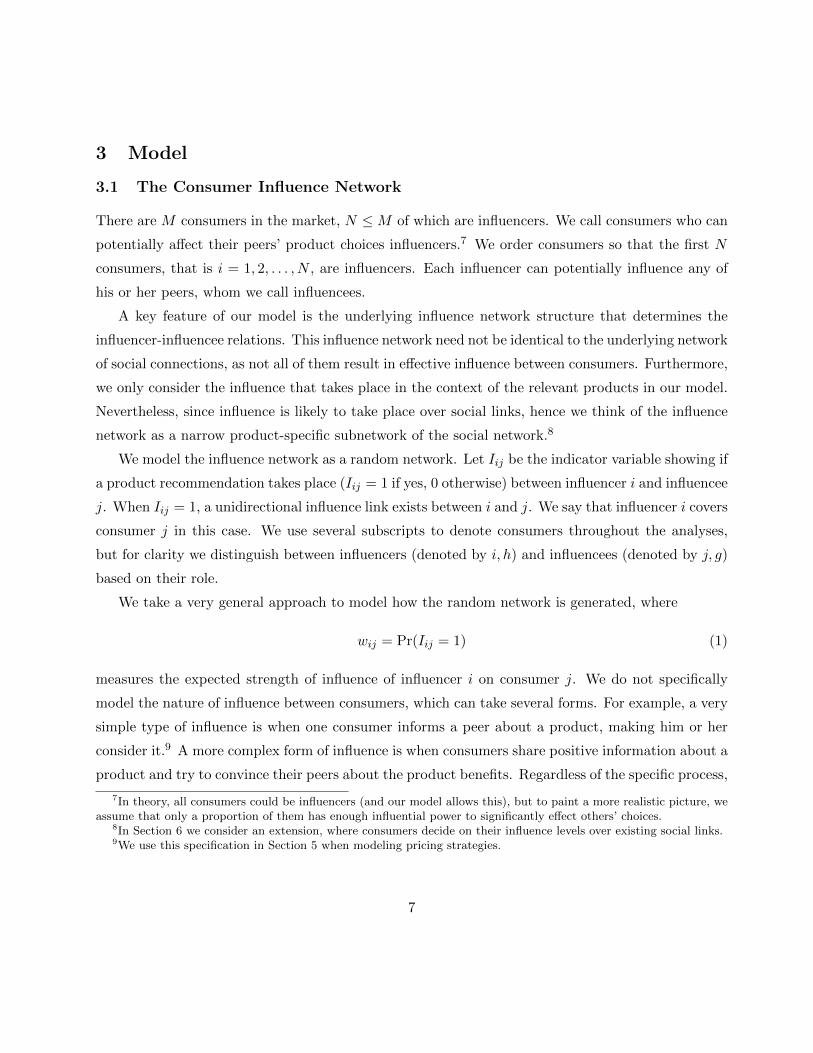
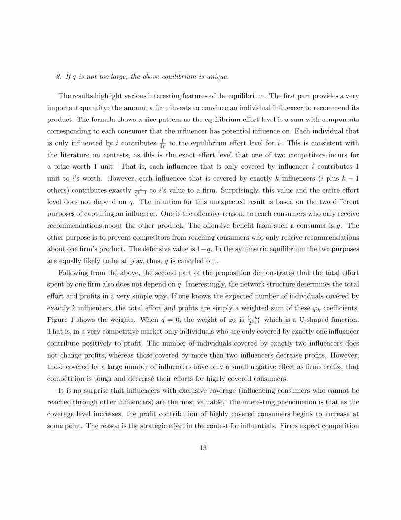
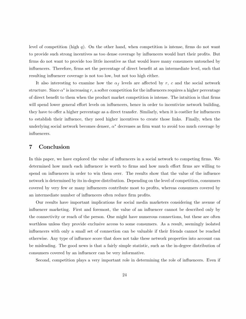
Figure 1 shows the weights. When q = 0, the weight of ϕk is 2−kr2k+1 which is a U-shaped function.

That is, in a very competitive market only individuals who are only covered by exactly one influencer

contribute positively to profit. The number of individuals covered by exactly two influencers does

not change profits, whereas those covered by more than two influencers decrease profits. However,

those covered by a large number of influencers have only a small negative effect as firms realize that

competition is tough and decrease their efforts for highly covered consumers.

It is no surprise that influencers with exclusive coverage (influencing consumers who cannot be

reached through other influencers) are the most valuable. The interesting phenomenon is that as the

coverage level increases, the profit contribution of highly covered consumers begins to increase at

some point. The reason is the strategic effect in the contest for influentials. Firms expect competition

13

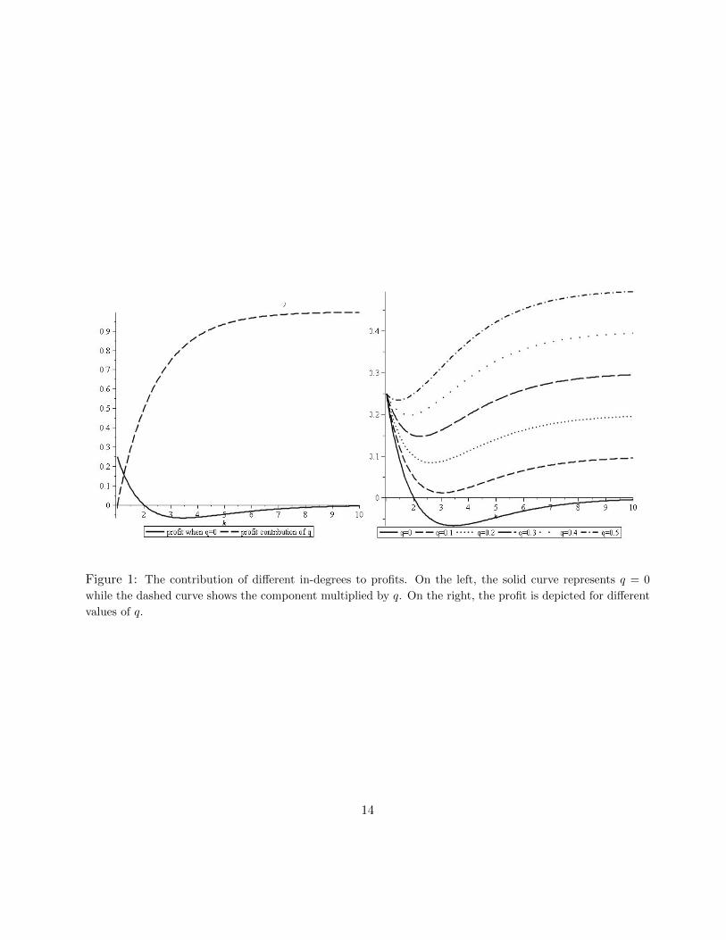
Figure 1: The contribution of different in-degrees to profits. On the left, the solid curve represents q = 0

while the dashed curve shows the component multiplied by q. On the right, the profit is depicted for different

values of q.

14

to be tough for influencers covering highly covered consumers and they cut back on their effort to

capture them. The reduction in effort exceeds the reduction in revenue for highly covered customers,

leading to the U-shaped curve. In particular, when q > 0 the profit contribution of highly covered

individuals changes in an interesting way. As k → ∞, the contribution of a consumer covered by k

influencers converges to q. Despite the reduced incentives to invest, these consumers contribute to

profits positively. As they most likely receive recommendations about both products, they yield a

profit of q to each firm.

It is worthwhile to examine how the two parameters measuring competition affect the results.

Recall that q measures the softness of the product market competition, whereas r measures the

softness of the competition for winning over influencers. As one would expect, profits are increasing

in both r and q. As competition becomes softer in either area, firms are better off. However, the

value of consumers with different in-degrees changes in an interesting way with these parameters as

the following corollary summarizes.

Corollary 1

1. There exists a k such that consumers covered by k > k influencers contribute to profits more

than those covered by one influencer if and only if q > 12 −

14r .

2. Consumers covered by exactly b2(1 + (1− 2q)r)c influencers contribute the least to firm profits.

Their contribution is negative when q and r are low.

Firstly, since the profit contribution of a consumer covered by k influencers is a U-shaped function

of k, it is not clear which consumers are the most valuable to firms. As we show above, the consumers

who are worth more are either the ones covered by only one influencer or the ones covered by

all of them. If q > 12 −

14r , that is, if competition is generally soft (q and/or r are high), then

consumers covered by all influencers are the most valuable in their contribution to profits. When

competition either in the product market or for influencers is tough, then we get the opposite results

and influencers that have a large exclusive coverage are worth the most.

Secondly, consumers who are covered by an intermediate range of influencers are the least valu-

able to firms as firms have less incentive to win over influencers covering such consumers. When

competition is tough, firms will want to avoid these consumers and the influencers covering them

as they decrease profits. This result has the intriguing consequence that firms are better off when

15

these consumers exit the market. That is, firms not only have the incentive to differentiate between

influencers based on their coverage, but different consumers also provide different value to firms

based on their position in the network.

Our results also refute the conventional wisdom that denser networks are better for firms that

take advantage of word of mouth. Removing influence links can actually increase profits in certain

cases. In Section 6 we will investigate further how firms can incentivize influencers to establish the

optimal amount of links.

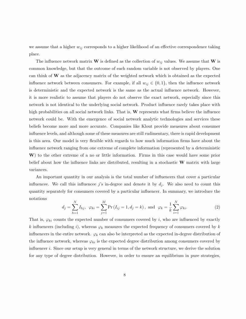
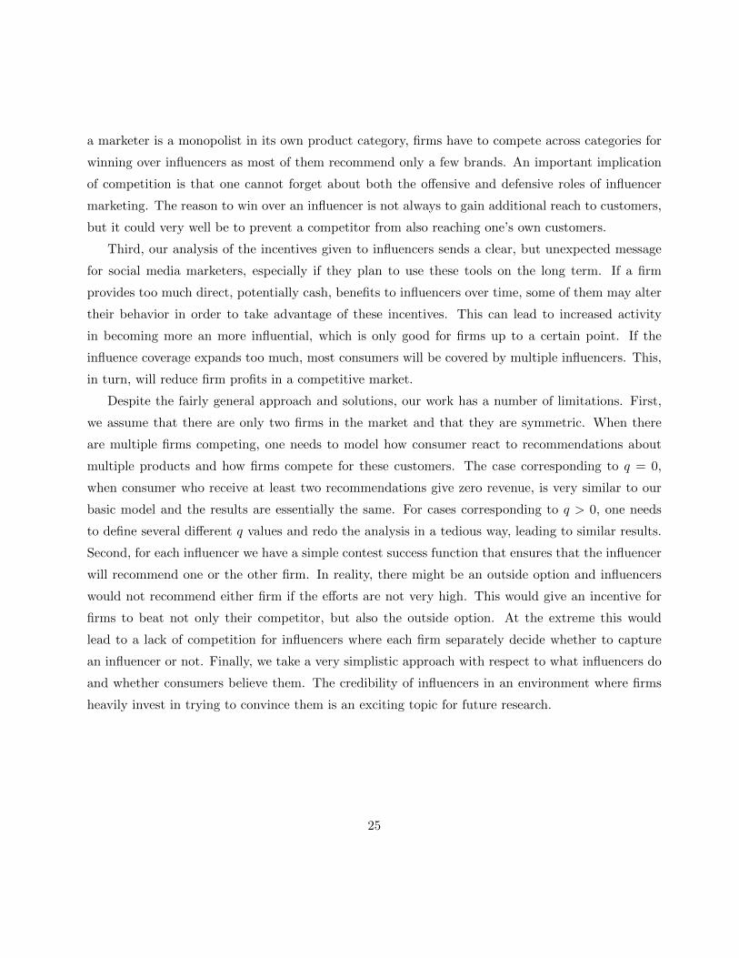
Finally, it is useful to uncover what are the optimal influence networks that firms profit the most

from. When q is low (< 12 −

14r ), firms would naturally prefer to avoid all competition and, at the

same time, cover all consumers. Hence, the optimal influence network is one where each consumer

is covered by exactly one influencer. This is a very specific network that is unlikely to be formed

in reality. A more realistic setting is when the density of the network is given and we would like

to determine the optimal network given the density. Fixing the total number of expected links, as∑Ni=1

∑j = 1Mwij = σ > M , for a given number of N also fixes the density at σ/N . When q is

low, the optimal network will have σ−MN−1 consumers covered by all influencers and the remaining

consumers covered by exactly one influencer. Figure 2 shows such an optimal network, where a core

of consumers are highly influenced and the rest are relatively isolated.

5 Influence, Consideration, and Prices

In our basic model we took a generic, but simplified approach to model the nature of influence and

competition. We assumed that firms made a fixed amount of profit per consumer which depended on

whether consumers received recommendations about only one or both products. Here, we extend the

model to incorporate the pricing decisions. To do so, we model the process of product recommenda-

tions between consumers in more detail. If a consumer receives product recommendations from an

influencer, the recommended product will enter his/her consideration set with some probability. To

account for the impact of multiple recommendations, we use the function 0 ≤ γ(`) ≤ 1 to denote the

probability that a consumer receiving exactly ` recommendations about a product considers it.

Each consumer has a reservation price normalized to 1 for each product. If there is only one

product in the consumer’s consideration set, s/he purchases that product as long as the price does

not exceed his or her reservation price. When there are multiple products in his or her consideration

16

Figure 2: Optimal influence network for firms

set, the consumer chooses the lowest priced product.

We also include firms’ pricing decisions in the model. Firms set their prices after the efforts for

influencers have been set and committed to.13 We assume that firms are able to price discriminate14

and set a different price pfj for each consumer j. Personalized pricing is more and more common in

practice,15 and the phenomenon has been studied in academia (Chen and Iyer 2002, Zhang 2011).

In order to customize prices firms do not have to identify all of the individual customers and exactly

determine their willingness to pay.16 Consistently, we assume that firms only have limited knowledge

in the pricing stage. They posses the exact same information about consumers as they have in

the first stage, namely the random influence network. When the network is stochastic, this leads

to considerable uncertainty with respect to a particular consumer’s consideration set, making it

13This is consistent with the advertising literature, where advertising decisions typically precede pricing.14Formally, we only need that firms are able to discriminate between different types of consumers: those who have

different number of influencers covering them. Furthermore, even if firms have to charge the same prices for allconsumers the results are not too different. For example, if there are only two influencers, the results are identical.

15“Shopper Alert: Price May Drop for You Alone”, New York Times, August 9, 201216“Web sites change prices based on customers’ habits”’CNN, June 24, 2005

17

impossible to extract all the surplus.

As before, we expect a symmetric equilibrium in firm efforts which leads to randomness in which

firm the influencer will recommend. Also, the influence network itself is random resulting in uncer-

tainty about what recommendations consumers receive. Consistently with our previous modeling

concept, we assume that firms cannot observe individual recommendations.17. Given all the uncer-

tainty, it is easy to see that there is no pure-strategy equilibrium in the pricing stage: Since there

is a positive likelihood that consumers consider both products, but also that they consider only

one product, we find an equilibrium with mixed strategies in pricing, similarly to Varian (1980)

and Narasimhan (1988). The following proposition describes the prices and the effort levels in the

unique symmetric equilibrium that comprises of pure effort strategies. Note that we define a Sk(t)

generating function in the proposition to simplify notation, where t takes the value of 0 or 1.

Proposition 2

1. The equilibrium effort level for firm f and influencer i is

efi =1

4r

∞∑k=1

ϕki

(4

kSk(1)− 2Sk(0)

), where Sk(t) =

k∑`=0

(k`

)γ(`)(1− γ(k − `))`t

2k.

2. The total effort levels and the profits are

M∑i=1

efi =1

4r

∞∑k=1

ϕk(4Sk(1)− 2kSk(0)), πf =∞∑k=1

ϕk

((1 +

k

2r

)Sk(0)− Sk(1)

r

).

3. The price pfj is a random variable with support[

αα+β , 1

]and p.d.f. g(p) = α

βp2where

α =

∞∑k=1

Pr(dj = k)Sk(0), β =

∞∑k=1

Pr(dj = k)

k∑`=0

(k`

)γ(`)γ(k − `)

2k

The results demonstrate how the effort levels depend on the degree distribution, similarly to the

basic model. Given the more general setup, the coefficients corresponding to the value of a consumer

covered by k influencers can be derived from the γ function as given by the Sk() formulas. To better

demonstrate the power of our results, we present two examples. The first example shows that our

17This assumption will not affect the decision on efforts, but will impact pricing. If firms can observe more, they willbe able to price discriminate more

18

basic model is a special case of this general setting, whereas the second example presents a slightly

different, but very realistic case.

Example 1 (First impression) Suppose γ(0) = 0 and γ(`) = γ > 0 for ` > 0. Then the equilibrium

effort levels and profits in Proposition 2 correspond to those in Proposition 1 with q = 1− γ.

The influence mechanism defined in this example is a very simple one: the first recommendation

a consumer receives about a product makes him/her consider a product with probability γ. Fur-

ther recommendations about a product do not increase the probability of consideration. This setting

captures a situation where first impressions matter overwhelmingly: for example when the recommen-

dation contains a simple piece of information that makes the consumer either consider the product

or not. Further recommendations containing the same information do not increase the likelihood of

consideration. An extreme example is γ = 1, when the information contained in the recommenda-

tion can be simply thought of as the existence of the product akin to the well known informative

advertising models. Substituting into the formulas reveals that Sk(0) = γ(1 − γ) + γ2

2k−1 − γ2k

and

Sk(1) = kγ(1−γ)2 + γ2k

2kwhich, in the case of γ = 1, exactly reproduces the results of Proposition 1

with q = 0. This is not surprising in the sense that when influencers simply make other consumers

aware of a product the price competition is intense for those who consider both products. When

γ < 1, the results are also reproduce those in Proposition 1. The corresponding q is 1 − γ, but we

also have to multiply all efforts and profits with γ to account for the reduced likelihood that any

consumer will consider the product.

It is also interesting to examine the prices. The equilibrium price distribution shows that firms set

random prices up to 1 starting at an intermediate value for each consumer. The size of the interval and

thus the overall level of prices depends on how many influencers cover the consumer. Given the γ()

function specified in the example, we obtain α =∑∞

k=1 Pr(dj = k)(γ(1− γ) + γ2

2k−1 − γ2k

)and β =∑∞

k=1 Pr(dj = k)(γ2 − γ2

2k−1

)suggesting two effects. First, prices generally increase as γ decreases

due to the softened price competition as less and less consumers consider both products, consistently

with q = 1 − γ decreasing with γ. Secondly, prices also depend on the number of influencers

that cover a consumer. As a consumer is covered by more influencers, it is more likely that this

consumer considers both products intensifying price competition and reducing prices. Consistently

with the results of Proposition 1, firms will thus invest less in influencers with highly covered followers

19

regardless of the value of q (and regardless of γ here). Even though prices go down as a function of

coverage, they never reach zero (as long as γ < 1), even if a consumer is covered by many influencers.

As a result, lower prices do not always hurt firms. When γ is sufficiently low and consumers are

not likely to consider a recommended product, increased coverage by influencers lowers prices, but

increases profits at the same time. The intuition follows from a combination of two strategic effects.

On one hand, increased coverage results in tougher price competition and lower prices. On the other

hand, high coverage leads to careful investments in the effort to convince influentials, leading to less

wasteful spending.

Clearly, the influence mechanism in Example 1 has extremely decreasing returns for additional

recommendations as γ() is very concave. Let us consider another example.

Example 2 (Cumulative influence) Suppose γ(`) = 1 − (1 − γ)` with γ > 0. Then Sk(0) = (1 −γ/2)k − (1− γ)k and Sk(1) = k

2

((1− γ/2)k−1 − (1− γ)k

)Subsequent recommendations for the same product can have a positive effect on consideration.

For example, when influencers convey more complex information, every new piece of information

can make influencees consider the product. Even more so, if recommendations involve some sort

of social pressure or network effects, where more recommendations lead to an increased likelihood

of consideration (as in Katona et al. (2011)). The results in this case are somewhat different. In

contrast to the case where first impressions matter the most, price competition gets very intense for

consumers covered by many influencers, prices tending to zero. This leads to a pattern similar to

that in Proposition 1 with q = 0. Deriving the profit reveals that

πf =∞∑k=1

ϕk

((1− γ/2)k−1

(1− γ/2

(1 +

k

2r

))− (1− γ)k

),

which results in positive profit contribution only for consumers covered by a few influencers. Con-

sumers covered by more will reduce profits, but the decline will be slower as γ decreases.

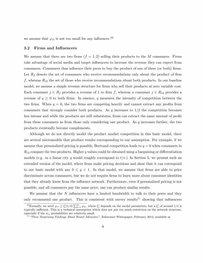
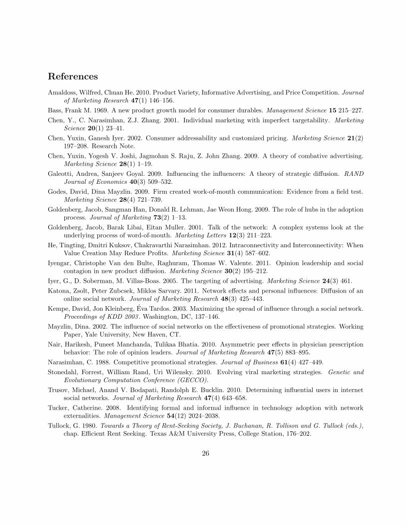
Comparing Examples 1 and 2 shows an interesting pattern. For γ = 1 the results are identical,

but for γ < 1 there are important differences. In both cases, consumers covered by few influencers

are valuable, but highly covered consumers have opposing impact on profits in the two cases. When

the first recommendations matter the most, dense networks are more profitable for firms, whereas

in case of cumulative influence, dense network always reduce profits, but less so as density increases.

20

On the flipside, consumers covered by only a few influencers contribute to profits more in case of

cumulative influence. Figure 3 shows a comparison between profits in the two cases.

Figure 3: Firm profits under different influence mechanisms. On the left, r = 2, γ = 0.9. On the right

r = 2, γ = 0.7

6 Endogeneous Network Formation and Influencer Incentives

Throughout the paper, we have assumed that the influence network is exogenously given. However,

there is increasing pressure on consumers to become influential among their peers in order to get

perks and benefits from firms. Klout - the influence score tracking service - even created a Klout

Perks API that makes it easier for firms to offer perks to their highly influential customers.18 In this

section, we examine how endogenizing the influence network formation affects our results. We also

study how firms should incentivize consumers to build the influence network. As we shown in the

main model, firms sometimes do not want consumers to be too much connected to each other, hence

we study what the optimal level of these incentives are in different social networks.

18“Your Influence (and Klout Score) is Worth Money” - available at http://www.stateofsearch.com/your-influence-and-klout-score-is-worth-money/

21

First, we describe the network formation process. As before, we assume that there are N influ-

encers out of M consumers in the market.19 We assume that there is a network of social connections

between consumers that provide the basis for influence to take place. Let uij be an indicator of a

link, that is, uij = 1 if there is a link between consumers i and j and uij = 0 otherwise, forming

the underlying social network matrix U. Whenever an influencer i wants to establish an influence

link of wij , it can only be done through an underlying social link. In other words wij ≤ uij for all

(i, j) pairs. Exerting influence on another consumer is costly, we assume that the cost of building

an influence link of wij strength costs the influencer C(wij). For the sake of tractability, we assume

that the cost function is quadratic and is sufficiently high, that is, C(wi) = c2w

2ij with a sufficiently

high c parameter.20

In order for influencers to build their networks and attempt to influence their peers, they have to

receive some benefit. We assume that this benefit comes directly from firms. When firm f exerts efi

effort to convince influencer i, some of this effort directly benefits influencer i as a monetary transfer.

The parameter αf measures the percentage of the effort efi that directly goes to the influencer. That

is, in our model influencer i receives a payment of αfefi from firm f . In reality this payment does

not have to be cash, instead it can be in the form of a rebate, points for future purchases, or simply

a price reduction. We do not model the exact nature of the payment, our assumption only specifies

that αfefi directly increases i’s utility, whereas the remaining (1−αf )efi does not change i’s utility,

only his or her probability to recommend firm f .

We assume that the above decisions take place in the following sequence. First, firms simultane-

ously announce and commit to αf , the percentage of effort that directly benefits influencers. Second,

influencers simultaneously build the network by selecting each consumer they want to influence and

the strength of the relationship. Third, firms simultaneously determine their effort levels, exactly

as in Section 3. As before, we are looking for equilibria that are symmetric with respect to the

firm strategies and we also require subgame-perfection. We first determine the possible equilibrium

networks for fixed αf .

Proposition 3 For fixed α1 and α2 values, a W random influence network is an equilibrium outcome

19An alternative approach is to assume that becoming an influencer is costly and to also endogenize the decision ofeach consumer to become an influencer. The results, however, would be similar.

20This ensures that wij < 1 in equilibrium.

22

if and only if each wij satisfies.

(1− wij/2)(∑N

g=1 ugj)−1

wij=

4rc

α1 + α2.

Thus, the equilibrium wij is decreasing in r, c, (∑N

g=1 ugj)− 1, and increasing in α1,α2.

The proposition shows us the equilibrium influence network structure. Influence takes place

over existing social connections, but with varying strength. How hard influencers try to influence

a consumer depends on his/her position in the social network. What determines the strength of

incoming influence links for a consumer is the number of influencers that the consumer is connected

to in the social network. Interestingly, consumers with connections to more influencers will be

influenced to a lesser extent. The intuition for this results is that the competition between firms

trickles down to the level of influencers who get lower benefits from consumers for which firms

compete more intensely.

The proposition also sheds light on the relationship between the social network and influence

network in our model. While the social network is potentially dense with most nodes having tens

or hundreds of connections, the influence network is typically much sparser, especially when influ-

encing someone is costly. The degree distribution of the influence network is thus shifted towards

lower degrees compared to the social network, with much more consumers influenced by only a few

influencers.

Another important implication of the proposition is that the incentives given by firms change

the structure of the influence network. The strength of all influence links increases with α1 and α2.

In other words, firms can incentivize influencers to form stronger links by increasing the portion of

their effort that is a direct transfer to influencers.

Corollary 2 In any symmetric equilibrium α1 = α2 = α∗ > 0 holds. α1 = α2 = α∗ = 1 is an

equilibrium outcome if and only if q is high or a high proportion of consumers have only one social

connection.

The result shows a surprising pattern. When the market is not very competitive, firms spend

all their effort on directly increasing the utility of influencers. The reason is that a high percentage

of direct payoff incentivizes influencers to build a dense network that benefits firms given the low

23

level of competition (high q). On the other hand, when competition is intense, firms do not want

to provide such strong incentives as too dense coverage by influencers would hurt their profits. But

firms do not want to provide too little incentive as that would leave many consumers untouched by

influencers. Therefore, firms set the percentage of direct benefit at an intermediate level, such that

resulting influencer coverage is not too low, but not too high either.

It also interesting to examine how the αf levels are affected by r, c and the social network

structure. Since α∗ is increasing r, a softer competition for the influencers requires a higher percentage

of direct benefit to them when the product market competition is intense. The intuition is that firms

will spend lower general effort levels on influencers, hence in order to incentivize network building,

they have to offer a higher percentage as a direct transfer. Similarly, when it is costlier for influencers

to establish their influence, they need higher incentives to create those links. Finally, when the

underlying social network becomes denser, α∗ decreases as firm want to avoid too much coverage by

influencers.

7 Conclusion

In this paper, we have explored the value of influencers in a social network to competing firms. We

determined how much each influencer is worth to firms and how much effort firms are willing to

spend on influencers in order to win them over. The results show that the value of the influence

network is determined by its in-degree distribution. Depending on the level of competition, consumers

covered by very few or many influencers contribute most to profits, whereas consumers covered by

an intermediate number of influencers often reduce firm profits.

Our results have important implications for social media marketers considering the avenue of

influencer marketing. First and foremost, the value of an influencer cannot be described only by

the connectivity or reach of the person. One might have numerous connections, but these are often

worthless unless they provide exclusive access to some consumers. As a result, seemingly isolated

influencers with only a small set of connection can be valuable if their friends cannot be reached

otherwise. Any type of influence score that does not take these network properties into account can

be misleading. The good news is that a fairly simple statistic, such as the in-degree distribution of

consumers covered by an influencer can be very informative.

Second, competition plays a very important role in determining the role of influencers. Even if

24

a marketer is a monopolist in its own product category, firms have to compete across categories for

winning over influencers as most of them recommend only a few brands. An important implication

of competition is that one cannot forget about both the offensive and defensive roles of influencer

marketing. The reason to win over an influencer is not always to gain additional reach to customers,

but it could very well be to prevent a competitor from also reaching one’s own customers.

Third, our analysis of the incentives given to influencers sends a clear, but unexpected message

for social media marketers, especially if they plan to use these tools on the long term. If a firm

provides too much direct, potentially cash, benefits to influencers over time, some of them may alter

their behavior in order to take advantage of these incentives. This can lead to increased activity

in becoming more an more influential, which is only good for firms up to a certain point. If the

influence coverage expands too much, most consumers will be covered by multiple influencers. This,

in turn, will reduce firm profits in a competitive market.

Despite the fairly general approach and solutions, our work has a number of limitations. First,

we assume that there are only two firms in the market and that they are symmetric. When there

are multiple firms competing, one needs to model how consumer react to recommendations about

multiple products and how firms compete for these customers. The case corresponding to q = 0,

when consumer who receive at least two recommendations give zero revenue, is very similar to our

basic model and the results are essentially the same. For cases corresponding to q > 0, one needs

to define several different q values and redo the analysis in a tedious way, leading to similar results.

Second, for each influencer we have a simple contest success function that ensures that the influencer

will recommend one or the other firm. In reality, there might be an outside option and influencers

would not recommend either firm if the efforts are not very high. This would give an incentive for

firms to beat not only their competitor, but also the outside option. At the extreme this would

lead to a lack of competition for influencers where each firm separately decide whether to capture

an influencer or not. Finally, we take a very simplistic approach with respect to what influencers do

and whether consumers believe them. The credibility of influencers in an environment where firms

heavily invest in trying to convince them is an exciting topic for future research.

25

References

Amaldoss, Wilfred, Chuan He. 2010. Product Variety, Informative Advertising, and Price Competition. Journalof Marketing Research 47(1) 146–156.

Bass, Frank M. 1969. A new product growth model for consumer durables. Management Science 15 215–227.

Chen, Y., C. Narasimhan, Z.J. Zhang. 2001. Individual marketing with imperfect targetability. MarketingScience 20(1) 23–41.

Chen, Yuxin, Ganesh Iyer. 2002. Consumer addressability and customized pricing. Marketing Science 21(2)197–208. Research Note.

Chen, Yuxin, Yogesh V. Joshi, Jagmohan S. Raju, Z. John Zhang. 2009. A theory of combative advertising.Marketing Science 28(1) 1–19.

Galeotti, Andrea, Sanjeev Goyal. 2009. Influencing the influencers: A theory of strategic diffusion. RANDJournal of Economics 40(3) 509–532.

Godes, David, Dina Mayzlin. 2009. Firm created work-of-mouth communication: Evidence from a field test.Marketing Science 28(4) 721–739.

Goldenberg, Jacob, Sangman Han, Donald R. Lehman, Jae Weon Hong. 2009. The role of hubs in the adoptionprocess. Journal of Marketing 73(2) 1–13.

Goldenberg, Jacob, Barak Libai, Eitan Muller. 2001. Talk of the network: A complex systems look at theunderlying process of word-of-mouth. Marketing Letters 12(3) 211–223.

He, Tingting, Dmitri Kuksov, Chakravarthi Narasimhan. 2012. Intraconnectivity and Interconnectivity: WhenValue Creation May Reduce Profits. Marketing Science 31(4) 587–602.

Iyengar, Christophe Van den Bulte, Raghuram, Thomas W. Valente. 2011. Opinion leadership and socialcontagion in new product diffusion. Marketing Science 30(2) 195–212.

Iyer, G., D. Soberman, M. Villas-Boas. 2005. The targeting of advertising. Marketing Science 24(3) 461.

Katona, Zsolt, Peter Zubcsek, Miklos Sarvary. 2011. Network effects and personal influences: Diffusion of anonline social network. Journal of Marketing Research 48(3) 425–443.

Kempe, David, Jon Kleinberg, Eva Tardos. 2003. Maximizing the spread of influence through a social network.Proceedings of KDD 2003 . Washington, DC, 137–146.

Mayzlin, Dina. 2002. The influence of social networks on the effectiveness of promotional strategies. WorkingPaper, Yale University, New Haven, CT.

Nair, Harikesh, Puneet Manchanda, Tulikaa Bhatia. 2010. Asymmetric peer effects in physician prescriptionbehavior: The role of opinion leaders. Journal of Marketing Research 47(5) 883–895.

Narasimhan, C. 1988. Competitive promotional strategies. Journal of Business 61(4) 427–449.

Stonedahl, Forrest, William Rand, Uri Wilensky. 2010. Evolving viral marketing strategies. Genetic andEvolutionary Computation Conference (GECCO).

Trusov, Michael, Anand V. Bodapati, Randolph E. Bucklin. 2010. Determining influential users in internetsocial networks. Journal of Marketing Research 47(4) 643–658.

Tucker, Catherine. 2008. Identifying formal and informal influence in technology adoption with networkexternalities. Management Science 54(12) 2024–2038.

Tullock, G. 1980. Towards a Theory of Rent-Seeking Society, J. Buchanan, R. Tollison and G. Tullock (eds.),chap. Efficient Rent Seeking. Texas A&M University Press, College Station, 176–202.

26

Van den Bulte, Cristophe, Gary L. Lilien. 2001. Medical innovation revisited: Social contagion versus mar-keting effort. American Journal of Sociology 106(5) 1409–1435.

Varian, H.R. 1980. A model of sales. The American Economic Review 70(4) 651–659.

Yoganarasimhan, Hema. 2012. Impact of social network structure on content propagation: A study usingyoutube data. Quantitative Marketing and Economics 10 111–150.

Zhang, Juanjuan. 2011. The perils of behavior-based personalization. Marketing Science 30(1) 170–186.

Zubcsek, Peter, Miklos Sarvary. 2011. Advertising to a social network. Quantitative Marketing and Economics9(1) 71–107.

27

Appendix

Proof of Proposition 1: We first determine the individual effort levels that each firm puts

out for a given influencer i assuming that the equilibrium is symmetric. Equations (5)-(11) express

the profit as a function of efi, keeping all other effort levels fixed. We can do the same exercise for

both firms and see that

Eπ1 =e1/r1i

e1/r1i + e

1/r2i

vi − e1i + C1, Eπ2 =e1/r2i

e1/r1i + e

1/r2i

vi − e2i + C2, (12)

which is a symmetric Tullock-contest with value

vi =

∞∑k=1

ϕki2k−1

. (13)

Differentiating player 1’s profit with respect to e1i, we get

∂Eπ1∂e1i

=e1/r−11i e

1/r2i

r(e1/r1i + e

1/r2i

)2 vi − 1 (14)

The expected profit is concave in e1i, hence the F.O.C gives the unique maximum for this single

variable. Setting e1i = e2i, the F.O.C becomes

vi4re1i

= 1 (15)

yielding e1i = vi4r which is the effort level given in the first part of the proposition. Note that r > 1/2

is necessary to ensure that the function in (12) have a positive derivative in 0. When r < 1/2, no

pure strategy equilibrium exist.

We have determined that the effort levels given above are optimal if the effort levels for all other

influentials are fixed. This is sufficient to show that the effort levels in equilibrium must be these,

but we need to also make sure that firms do not have an incentive to deviate by changing multiple

effort levels. That is, we need to check the second order condition for the maximization problem

involving all N variables for a given player. We show that the Hessian is negative definite, yielding

that player 1’s profit function has a maximum in the above identified equilibrium candidate (corner

solutions are ruled out since the derivative is always positive in a given effort variable when its set to

28

zero as long as r > 1/2). First, from (12) and (13) we get that when e1i = e2i the second derivatives

forming the diagonal of the Hessian are

∂2Eπ1∂e21i

= − 1

4re21i

∞∑k=1

ϕki2k−1

< 0.

When e1i = e2i and e1i = e2i, the (ij) off-diagonal element in the Hessian is

∂2Eπ1∂e1i∂e1j

=1− 2q

16r2e1ie1j

∞∑k=2

ϕk(i,j)

2k−2≤ 1− 2q

8r2e1ie1j

( ∞∑k=2

ϕki2k−1

+

∞∑k=2

ϕkj2k−1

),

where ϕk(i,j) denotes the number of consumers covered by exactly k consumers among those whore

are covered by i and j. This is analogous to the definition of ϕki and it is clear that ϕk(i,j) ≤ ϕki and

ϕk(i,j) ≤ ϕkj . Furthermore, when ϕki is high enough the diagonal elements dominate the matrix. One

can then divide each row by the diagonal element to see that the matrix is negative definite, since

all the diagonal elements are −1 in the modified matrix and the off-diagonal elements are smaller

than any positive threshold when ϕki is high enough for all i.

For part 2, we need to simply sum the effort levels across all influencers. Recalling that∑N

i=1 ϕki =

kϕk, we easily get the first equation for∑N

i=1 efi. In order to determine profits, we need to calculate

the revenues. From a consumer covered by k influencers there are two possibilities firm 1 could

earn money. With probability 12k

, the consumer is in R1 and the revenue for firm 1 is 1. With

probability 1− 12k−1 the consumer is in R12 yielding a revenue of q. Therefore the total revenue for

firm 1 is 12k

+ q(1− 1

2k−1

). Subtracting the investment in effort, we obtain the profit as given in the

proposition.

For part 3, let G denote the game we are analyzing in the proposition. Let G′ denote a modified

game with 2N players, with two players for each influencer. The games G and G′ are identical, except

that in G′ we split each of the two players in G into N different players that set the N effort levels

separately. Each of the N players in G′ that correspond to player 1 in G gets the entire payoff player

gets in G. It is clear that the N players in G′ face the same maximization problem that player 1

in G for each variable. Therefore, any equilibrium of G also has to be an equilibrium of G′, but not

vice versa. However, if we show that G′ has a unique equilibrium in pure strategies G either has

no equilibrium or a unique equilibrium. In order to show that G′ has a unique equilibrium in pure

strategies, let us write the profit function of player 1 as

Eπ1 =∑

S⊆{1,...,N}

AS∏i∈S

P1i −N∑h=1

e1h. (16)

29

This formulation simply says that the revenue is a multinomial of P11, . . . , P1N with coefficients AS ,

where P1i =e1/r2i

e1/r1i +e

1/r2i

. Simple calculation shows that that when q is small enough all coefficients are

positive. All the players’ profit functions are concave in this case, yielding a unique equilibrium for

G′. Since we have already shown that G has at least one equilibrium, it must be unique.

Proof of Corollary 1: For part 1, Proposition 1 shows that the profit contribution of a

consumer covered by k influencers is

a(k) =2− k/r

2k+1+ q

2k−1 − 1

2k−1. (17)

This takes the value of 12 −

14r for k = 1 and increasingly converges to, but never reaches q as k →∞.

If q ≤ 12 −

14r , the maximum contribution is always for k = 1. If q > 1

2 −14r , let k denote the largest

solution of2− k/r

2k+1= q

2k−1 − 1

2k−1. (18)

For k > k we get that the RHS exceeds the LHS, completing the proof of part 1.

For part 2, further examining the a(k) function shows that it first decreases, has a unique mini-

mum then increases. To determine the minimum, we solve a(k) = a(k+1) yielding k = 1+2r(1−2q).

This is not necessarily an integer, but we know that the integer that minimizes a(k) is between k

and k + 1, yielding the stated formula.

Proof of Proposition 2: Since we are looking for a symmetric equilibrium, we first determine

the pricing strategies given symmetric firm effort levels. In a symmetric equilibrium, all influencers

recommend both firms with the same probability, which allows us to determine the likelihood that

consumer j considers both products (let us denote by β) or only one product (α). Given α and β

we can use the mixed strategy equilibrium derived by Varian (1980), Narasimhan (1988) as stated in

the proposition. First, to calculate α, let us assume that consumer j is covered by k influencers (this

happens with probability Pr(dj = k)). Let us also assume that ` of these k influencers recommend

product 1. The likelihood that consumer j considers only this product is then γ(`)(1 − γ(k − `)).Combining these probabilities for different values of ` yields the formula stated in the proposition

since the probability that ` out of k influencers recommend proudct 1 is(k`

)/2k. Similar calculations

give the value of β.

To derive the equilibrium effort levels, we follow the same lines as in the proof of Proposition

1. The value of winning over influencer i can be written as a sum over the consumers covered by i.

30

For a particular j consumer covered by exactly k influencers, the value is γ(`)(1− γ(k − `))− γ(`−1)(1−γ(k− `+ 1)) if the consumer receives firm 1’s recommendations from `−1 out of the the k−1

other influencers and and receivers firm 2’s recommendations from k − ` of them. The probability

that `− 1 of the other k− 1 influencers recommend product 1 is(k−1`−1)/2k−1. We can then write the

value of winning over influencer i as

vi =∞∑k=1

ϕki2k−1

k∑`=1

(k − 1

`− 1

)[γ(`)(1− γ(k − `))− γ(`− 1)(1− γ(k − `+ 1)] . (19)

Using the equality(k−1j−1)−(kj−1)

= 2j−kk

(kj

), we obtain

vi =∞∑k=1

ϕki2k−1

k∑`=0

(k

`

)2j − kk

γ(`)(1− γ(k − `)). (20)

As in the proof of Proposition 1, the equilibrium effort levels will be vi4r resulting in the formula

provided in the proposition.

Proof of Proposition 3: Influencers receive a fixed proportion of firms’ efforts. The payoff of

influencer i is

πinfli =α1 + α2

4r

∞∑k=1

ϕki2k−1

− c

2

M∑j=1

w2ij

Since the above is additively separable for the different consumers covered by the influencer, let us

separate the part for an individual consumer j who is connected to i (that is, uij = 1) as

wijα1 + α2

4r

∞∑k=1

Pr(j is covered by k − 1 other influencers)

2k−1− c

2w2ij

Note that all influencers trying to cover consumer j maximize a similar payoff function and due

to the concavity, it is easy to see that the equilibrium is unique, and - as we show - symmetric. If

wgj = w(d) for all g that have a social connection to j (such that ugj = 1) then Pr(j is covered by k−1 other influencers) =

(d−1k−1)w(d)k−1(1 − w(d))d−k, where d =

∑Ng=1 uij . Summing these, we get

(1− w/2)d−1, thus the first order condition for influencer i and consumer j becomes

α1 + α2

4r(1− w/2)d−1 − cwij = 0

This completes the proof if we substitute wij = w(d), as there is a symmetric equilibrium that must

be unique.

31

Proof of Corollary 2: The profit firms can be calculated as a sum of profits made on each

consumer. For a consumer that has d connections in the social network, we can calculate the

probability that s/he will be covered by k influencers from the proof of Proposition 3 as(dk

)w(d)k(1−

w(d))d−k. Using these probabilities, we can write the profit contribution of a consumer with d social

ties as

π(d) =∑k=1

(d

k

)w(d)k(1− w(d))d−k

(2− k/r

2k+1+ q

2k − 1

2k

).

The profit function maximized by firms is then∑∞

d=1 ϕ′dπ(d), where ϕ′d denotes the number of

consumers with exactly d social ties, that is, the degree distribution of the underlying social network.

When q = 0, simple calculations show that

π(d) =

(1− w(d)

2

d−1)(

1− w(d)

2− dw(d)

4r

)− (1− w(d))d.

With the exception of d = 1, one can show that π(d) is increasing in w for small positive values of w,

then decreasing until it becomes negative at 4rd+2r . A linear combination of different π(d)’s exhibits a

similar pattern as long as the weight of π(1) is not too high (when there are not too many consumers

covered by only one influencer). Therefore, as long as q = 0, α1 + α2 = 0 cannot be optimal for

firms, as that would result in w(d) = 0 and both firms would want to deviate by increasing their αf .

To see when α1 = α2 = 1 is an equilibrium, we need to examine the π(d) functions again. When

q = 1/2, all π(d) functions are increasing in w, therefore firms will want to achieve the highest

possible w(d) values by setting α1 = α2 = 1. The same happens when π(1) has a very high weight in

the overall profit function. If q is not high and a low proportion of consumers are connected to one

influencer, the profit function will be decreasing at interior (less than 1 α values), since we assumed

the cost parameter c to be high enough.

32