How Much is a Win Worth?

An Application to Intercollegiate Athletics

Doug J. Chung*

August 2015

 

                                                            * Doug J. Chung is an assistant professor of business administration at Harvard Business School (dchung@hbs.edu). The author thanks the department editor, associate editor, and two anonymous reviewers for their constructive feedback during the review process. The author also thanks David E. Bell, Silvia Bellezza, Neil Bendle, T. Colin Campbell, Thomas Dotzel, Katja Frey, Uma R. Karmarkar, Vineet Kumar, Michael I. Norton, Byoung Gun Park, Alex Petkevich, Shelle M. Santana, and the seminar participants at Boston College, Kansas State University, Texas A&M University, and the University of South Carolina, in addition to the conference participants at the 2013 INFORMS Marketing Science Conference for their comments and suggestions. The author wants to give a very special thanks to his father, Towoong Chung, for introducing him to the exciting world of intercollegiate athletics during the author’s childhood and thus, as acknowledgement, has used the plural form (we, us, our, etc.) throughout the text of this manuscript.

 

How Much is a Win Worth?

An Application to Intercollegiate Athletics

Abstract

Intercollegiate athletics in the United States have become a multibillion-dollar industry

over the past several decades. In this study, we investigate the short- and long-term direct

monetary effects of operating a winning athletics program for an academic institution of higher

education. We construct a unique panel dataset from multiple sources and utilize the latest

dynamic panel data estimation methods to account for heterogeneity while also addressing

endogeneity concerns. We find that success in men’s football and basketball has a significant

impact on a school’s respective football and basketball revenues; however, the effect is different

based on the type of school. We find that regular season wins in football account for most of the

increase in revenue for established schools whereas invitations to prestigious postseason bowl

games play a big part for less-established schools. Furthermore, we find that student population

and education quality dissipate the effect of athletic success on monetary payoffs. We find that

success in basketball carries over more from the past than in football with additional

contemporaneous marginal effects for established schools. We do find, however, that past athletic

success carries over significantly to the present in both football and basketball, suggesting the

significance of the long-term monetary effect of athletic success to many academic institutions in

the United States.

Key words: dynamic panel data, heterogeneity, instrumental variables, intercollegiate athletics,

educational finance, entertainment marketing.

1  

1. Introduction

In the late 1800s, Rutgers and Princeton were intense rivals. Separated by a mere 20 miles,

the two universities had, for years, battled for possession of an old Revolutionary War cannon,

making night forays to surreptitiously transport the cannon from one campus to another.

Princeton eventually settled that debate by sinking the gun in several feet of concrete. Further

rubbing salt into the wound, in that same year, Princeton beat Rutgers in baseball by a merciless

score of 40–2. Rutgers, hoping to square things up, challenged its rival to a game with rules that

resembled those of English football and rugby. Princeton accepted the challenge and, on

November 6, 1869—on a field where present-day Rutgers University’s gymnasium stands in New

Brunswick, New Jersey—the first intercollegiate American football game was played. Rutgers won

that game 6–4, ushering in a new era in U.S. culture.1

Ever since, academic institutions have participated in intercollegiate athletics as a way to

boost pride within the student and alumni communities, to increase morale, and to promote

diversity. The mission of the National Collegiate Athletic Association (NCAA), the governing

body of intercollegiate athletics, is “to govern competition in a fair, safe, equitable, and

sportsmanlike manner, and to integrate intercollegiate athletics into higher education so that the

educational experience of the student-athlete is paramount.” Among the NCAA’s core values are

integrity, sportsmanship, diversity, the pursuit of excellence in both academics and athletics, and

the enhancement of a sense of community and the strengthening of the identity of member

institutions.

While those objectives and values are still emphasized, the landscape of intercollegiate

athletics has changed substantially over the past several decades. Today’s intercollegiate athletics

has become a multibillion-dollar industry, generating large amounts of revenue for the

participating institutions. During the 2013–14 academic year, 67 schools made more than $50

                                                            1 Source: “Rutgers—The Birthplace of Intercollegiate Football,” www.scarletknights.com, Rutgers University Athletic Department. Although the first competitive intercollegiate sporting event was in rowing between Yale and Harvard Universities, which took place at Lake Winnipesaukee, New Hampshire, in 1852 (Lewis, 1970), it is men’s football and basketball that have captured the attention of the general public and, along with baseball, are thought of as the key sports programs that allowed intercollegiate athletics to thrive in the United States.

2  

million and the top 19 schools each generated more than $100 million in revenues through their

athletics programs (see Table 1). At the top of the list was the University of Texas at Austin,

with $161 million.2 Hence, intercollegiate athletics has become more than simply a tool to promote

scholarship and diversity. It has become commercialized and represents a key source of revenue for

many academic institutions.

<Table 1>

To better understand the dynamics of this high-profile and interesting industry, this study

investigates the likely components that affect monetary payoffs in intercollegiate athletics.

Specifically, it looks at the effect of winning (athletic success) and its short- and long-term impact

on revenues generated by the athletics programs of an academic institution of higher education.

Furthermore, we look at how the effect of winning, if any, differs between more-established

institutions and less-established ones. In addition, we look into the possible cross-promotional

effects of winning across sports, where success in one sport may spill over into higher revenues in

other sports. Finally, we look at what are some of the root causes that transform athletic success

into monetary payoffs.

This is a particularly salient topic to investigate in the current atmosphere of collegiate

athletics. There is an active nationwide debate on whether college student-athletes should be

paid—should the players share a piece of the revenue pie that they are creating on the field and

the court? A 2014 ruling by the National Labor Relations Board allowed Northwestern

University’s football team members to vote to be recognized as employees of the university, to

unionize, and be paid for their play. In addition, if recognized as employees, universities would

legally be liable for injuries incurred by student-athletes on the field.3 However, the NCAA did not

support that decision and has rules in place that prevent universities from paying their players.

                                                            2 Source: “The Equity in Athletics Data Analysis Cutting Tool,” Office of Postsecondary Education, U.S. Department of Education. 3 It is suggested that the term student-athlete was created by the NCAA in 1964 as a defense for adverse legal rulings such as workers’ compensation (Solomon, 2013). Typically, treatment for injuries on the field by student-athletes is covered while in school and not covered once they have graduated (Source: Real Sports with Bryant Gumbel, season 21, episode 3, Home Box Office).  

3  

Nonetheless, the debate continues, with some believing it will only be a matter of time before

some college athletes are compensated.

This research will provide policy makers the measures (by quantifying the value of athletic

success) to properly evaluate this issue, which would lead to better policies that will mutually

benefit schools and student-athletes across different types of schools. Specifically, our findings can

be used to structure an appropriate pay-for-play contract between schools and players when

deemed necessary. In addition, this research will help school administrators and marketers to

financially evaluate their athletics programs in order to properly determine investment amounts

by different types of sports.

Despite their growing level of popularity and the tremendous amounts of money involved,

intercollegiate athletics have generally received little attention in the academic literature. Several

studies have looked at the relation between athletic success and academics. Specifically,

McCormick and Tinsley (1987), Tucker and Amato (1993), Murphy and Trandel (1994), Mixon

(1995), Pope and Pope (2009), and Chung (2013) have investigated how athletic success can spill

over to influence admissions for institutions of higher education, commonly known as the “Flutie

Effect.”4 Furthermore, Lewis and Tripathi (2012) have examined the effect of investments in

collegiate athletics on school brand equity. In addition, Sigelman and Carter (1979), Sigelman and

Bookheimer (1983), and Baade and Sundberg (1996) have focused on the correlation between

athletic success and alumni donations. 5 However, to the best of our knowledge, the direct

monetary effect of having a successful athletics program has surprisingly not been explored in the

academic literature.

This study examines athletic success in two of the most popular sports (popular among

both students and the general public) in intercollegiate athletics: men’s football and basketball.

We compile a unique panel dataset from multiple sources that combines athletics success and

                                                            4 The “Flutie Effect” refers to the increase in exposure and prominence of an academic institution due to the success of its athletics programs. This effect is named after Boston College’s star quarterback Doug Flutie, who threw an extraordinary “Hail Mary” touchdown pass against the University of Miami to win a nationally televised game in 1984. That victory purportedly played a big role in the increase of applications to Boston College in the following years. For a detailed review of this literature, refer to Pope and Pope (2009) and Chung (2013). 5 For a detailed review of this literature and the literature on intercollegiate athletics in general, see Frank (2004).

4  

separate revenue data for each athletics program. We then take advantage of this panel structure

and utilize a dynamic estimation framework for our empirical strategy. Similar to professional

sports, a school’s athletics revenues can be highly affected by on-field performance, where better

performance generates enthusiasm and excitement, leading to higher ticket and merchandise sales.

In addition, students and alumni would want to bask in reflected glory (BIRG) by associating

themselves with a school’s athletic success (Cialdini et al., 1976). Furthermore, better performance

in previous seasons would generate excitement and expectations about the current season, and,

hence, the previous year’s performance would likely carry over and affect current sales. Thus, to

accommodate this dynamic process, we model a school’s athletics revenues as a function of

athletics goodwill that augments with current athletic success but which is allowed to decay over

time. This framework is similar to the advertising-as-investment model of Nerlove and Arrow

(1962) and, more generally, the dynamic panel data model of Balestra and Nerlove (1966). From

an estimation perspective, we apply the dynamic panel data methods of Arellano and Bond (1991),

Arellano and Bover (1995), and Blundell and Bond (1998). These methods are advantageous in

that they allow us to account for unobserved school heterogeneity while, at the same time, deal

with endogeneity concerns without relying on strictly exogenous instrumental variables.

Overall, we find that own success in a particular sport has a significant impact on own

revenue. That is, football and basketball success each leads to higher football and basketball

revenue, respectively. In football, we find that regular season wins account for most of the increase

in revenue for established schools whereas invitations to prestigious bowl games play a big part for

less-established schools. In basketball, we find the correlation between revenue and success in

terms of the fraction of wins to be linear with an added effect for established schools. Furthermore,

we find that the size of the student body and education quality dissolves the effect of athletic

success on monetary payoffs. We find that the success in basketball carries over more from the

past than in football. Nevertheless, we find a significant level of carryover from previous years’

athletic success in both basketball and football, indicating that the monetary gain from successful

athletics programs is not for just one season but for a more extensive period.

5  

The remainder of this paper is organized as follows. Section 2 presents the data, the

structure of intercollegiate athletics, and model-free evidence. Section 3 explains the model and

the corresponding empirical estimation strategy. Section 4 discusses the results, and Section 5

concludes.

2. Data and Model-Free Analysis

2.1. Data

We utilize multiple data sources to empirically investigate the effect of athletic success on

revenue generated by an academic institution of higher education. We obtained revenue data from

the Office of Postsecondary Education (OPE) Equity in Athletics Disclosure website database,

utilizing the Equity in Athletics Data Analysis Cutting Tool managed by the OPE of the U.S.

Department of Education. All postsecondary educational institutions that receive Title IV funding

(i.e., that participate in federal student aid programs) and have an intercollegiate athletics

program are required by the Equity in Athletics Disclosure Act to submit athletics-related data

annually. As explained by the OPE, the classification of revenue refers to all revenues attributable

to a particular intercollegiate athletics program. This includes ticket and luxury-box sales,

contributions from alumni and others, appearance guarantees and options, institutional royalties,

signage and other sponsorships, sport camps, student activity fees, state or other government

support, and any other revenues attributable to intercollegiate athletic activities for a particular

sport.6 We also obtained cost data with regards to each sport from the OPE. The analysis is

limited to eleven years (2003–2013) because the OPE revenue data starts in 2003. Data for

athletic success were collected through multiple public sources, mainly from the websites

Wikipedia and Sports-Reference. School characteristics, such as the size of the student body and

faculty-student ratio, were obtained from the Integrated Postsecondary Education Data System

(IPEDS), operated by the National Center for Educational Statistics (NCES). Finally, to control

for inflation, we used the consumer price index from the U.S. Bureau of Labor Statistics to

convert all monetary values to 2013 U.S. dollars.                                                             6 Source of definition: from “glossary of terms” on the Equity in Athletics Data Analysis Cutting Tool website.

6  

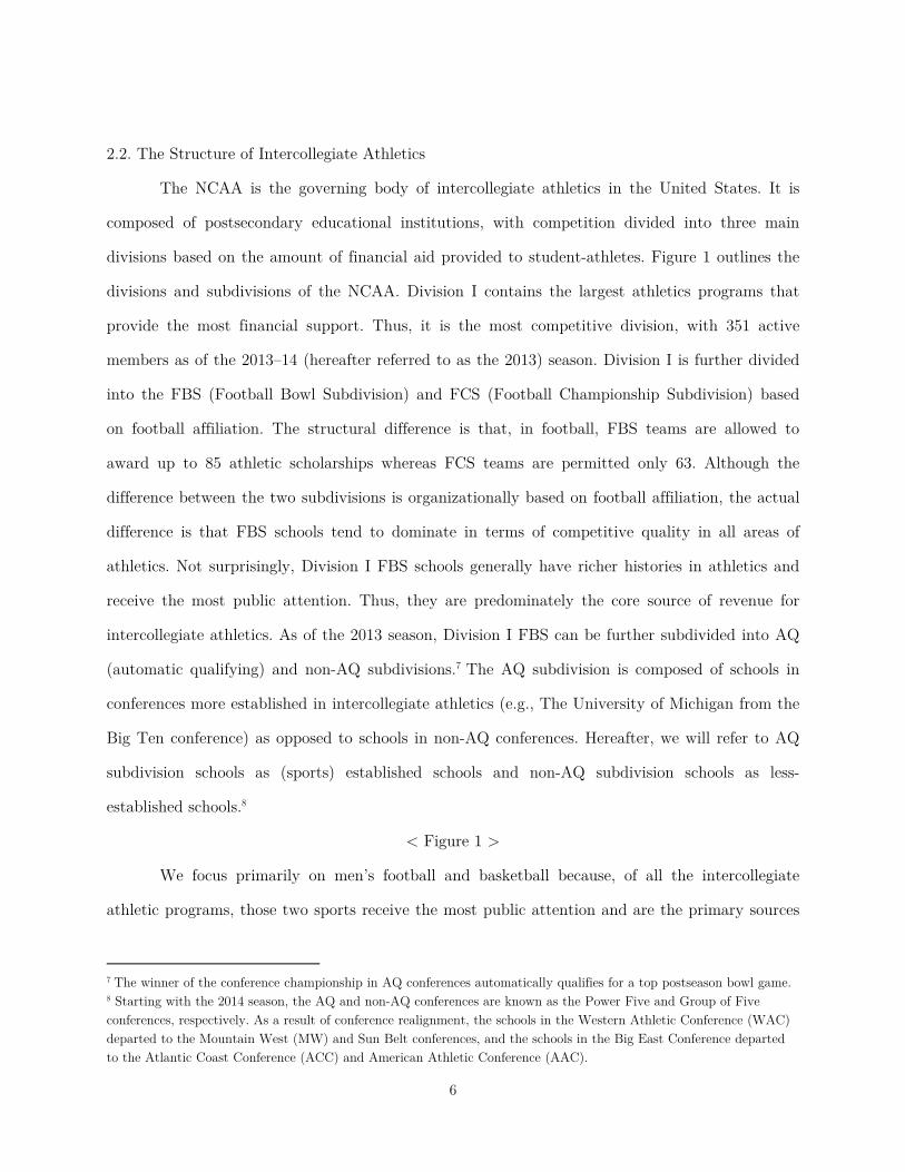
2.2. The Structure of Intercollegiate Athletics

The NCAA is the governing body of intercollegiate athletics in the United States. It is

composed of postsecondary educational institutions, with competition divided into three main

divisions based on the amount of financial aid provided to student-athletes. Figure 1 outlines the

divisions and subdivisions of the NCAA. Division I contains the largest athletics programs that

provide the most financial support. Thus, it is the most competitive division, with 351 active

members as of the 2013–14 (hereafter referred to as the 2013) season. Division I is further divided

into the FBS (Football Bowl Subdivision) and FCS (Football Championship Subdivision) based

on football affiliation. The structural difference is that, in football, FBS teams are allowed to

award up to 85 athletic scholarships whereas FCS teams are permitted only 63. Although the

difference between the two subdivisions is organizationally based on football affiliation, the actual

difference is that FBS schools tend to dominate in terms of competitive quality in all areas of

athletics. Not surprisingly, Division I FBS schools generally have richer histories in athletics and

receive the most public attention. Thus, they are predominately the core source of revenue for

intercollegiate athletics. As of the 2013 season, Division I FBS can be further subdivided into AQ

(automatic qualifying) and non-AQ subdivisions.7 The AQ subdivision is composed of schools in

conferences more established in intercollegiate athletics (e.g., The University of Michigan from the

Big Ten conference) as opposed to schools in non-AQ conferences. Hereafter, we will refer to AQ

subdivision schools as (sports) established schools and non-AQ subdivision schools as less-

established schools.8

< Figure 1 >

We focus primarily on men’s football and basketball because, of all the intercollegiate

athletic programs, those two sports receive the most public attention and are the primary sources

                                                            7 The winner of the conference championship in AQ conferences automatically qualifies for a top postseason bowl game. 8 Starting with the 2014 season, the AQ and non-AQ conferences are known as the Power Five and Group of Five conferences, respectively. As a result of conference realignment, the schools in the Western Athletic Conference (WAC) departed to the Mountain West (MW) and Sun Belt conferences, and the schools in the Big East Conference departed to the Atlantic Coast Conference (ACC) and American Athletic Conference (AAC).

7  

of revenue for each of their participating institutions.9 Furthermore, given the dominance of

Division I FBS, we focus our attention to the 117 schools that belong to this division.10 Table 2

shows the descriptive statistics of the revenue data. Three observations are worth noting from

Table 2. First, the range in revenues among the schools is large in both football and basketball.

The maximum and minimum revenues in football are $113 million and $800,000, respectively, and

the maximum and minimum in basketball are $44 million and $123,000, respectively. Second,

there is a large discrepancy between established and non-established schools in both football and

basketball, with established schools’ average revenue being more than four times that of their less-

established counterparts. Finally, football revenue greatly exceeds basketball revenue. Although

men’s basketball is popular, especially during the month of March with the NCAA basketball

tournament (popularly known as “March Madness”), revenues of basketball are dwarfed by that of

football.

< Table 2 >

Figure 2 shows the distribution of the ratio of football-to-basketball revenues for schools in the

sample data. Predominantly, the ratio is above one, with only three schools out of 117 having

lower ratios. The maximum ratio is 23.8 and the mean is 4.0, implying that, for a typical school,

football revenue is four times as large as basketball revenue.

< Figure 2 >

2.3. Model-free Evidence

Figures 3a and 3b show the empirical distribution of revenues by schools over the analysis

period. In terms of revenues in both football and basketball, the degree of heterogeneity among

the schools is enormous. What might be the key factor that affects this difference? The first thing

                                                            9 The college football and basketball seasons are described in greater detail in Section 3.1. 10 As of the 2013 season, there were 125 schools in Division I FBS. The three U.S. service academies—the U.S. Military Academy in West Point, the U.S. Naval Academy in Annapolis, and the U.S. Air Force Academy in Colorado Springs—did not report any revenue and, hence, were omitted from the sample. Also, we would need a minimum of three observations for our empirical strategy, thus, we omitted schools that joined the FBS after 2012. These schools were Georgia State University, Texas State University, University of Massachusetts, University of South Alabama, and the University of Texas at San Antonio.

8  

that comes to mind is the level of success of a particular team’s athletics program. Similar to

professional sports teams, success would be followed by enthusiasm and publicity, which would

likely lead to greater ticket and merchandise sales, endorsements, and alumni donations.

< Figure 3 >

Table 3 shows the descriptive statistics of several athletic success variables in basketball

and football across Division I FBS schools per season. The number of wins is based per season and

the fraction of wins is constructed such that the number of wins is divided by the total number of

games played in a season. The variable BCS (Bowl Championship Series) bowl represents the

fraction of schools invited to compete in one of the five prestigious postseason BCS bowl games.11

In football, we see that Division I FBS schools, on average, win about seven games per season and

eight percent of those get invited to compete in BCS bowl games. In basketball, schools win about

19 regular season games per season. For the postseason, 15 percent of the schools are invited to

play for the NCAA tournament and a mere two percent of them advance to the final 4 of the

tournament. Not surprisingly, in all categories of athletic success, AQ schools strictly outperform

in both football and basketball, reflecting the greater tradition and resources for intercollegiate

athletics among AQ schools.

< Table 3 >

Now, let us look into the possible correlation between revenues and athletic success.

Figures 4a and 4b show scatter plots of annual revenue on wins-per-season and the best-fitting

nonparametric smoothed polynomial with its 95-percent confidence interval shaded in gray for

basketball and football, respectively.

< Figure 4 >

From Figure 4a, one can see a clear positive correlation between the number of football wins and

its corresponding revenue. There is also a positive correlation between the number of basketball

wins and revenue, as shown in Figure 4b. Because there can be variations in the number of games

played in a season, one can argue that the fraction of wins per season, which takes into account                                                             11 The BCS is a selection system that chose the teams to play in prestigious postseason bowl games according to their regular season. These postseason bowl games were the Fiesta, Orange, Rose, and Sugar Bowls, as well as the BCS National Championship. The BCS system was replaced by a four-team playoff system as of 2014.

9  

the total number of games played, would be a better proxy for athletic success than the absolute

number of wins.12 Figure 5a and 5b show these relations. We can see the same trend as in Figure 4

but notice more precise correlation with smaller 95-percent confidence intervals.

< Figure 5 >

Although the above analyses presume a positive correlation between athletic success and

revenues, they can be misleading because they do not take into account school-specific

heterogeneity. To better understand the correlation between athletic success and revenues, we

would need to accommodate for differences across schools. Also, what might be other factors that

drive the revenues of a school’s athletics programs? Can revenues be a function of the status quo?

In other words, can revenues be a function of the relative increase in athletic success compared to

the previous season?

To more deeply understand the correlation between revenue and athletic success, and to

account for school heterogeneity, Figure 6 shows a scatter plot of the percentage change in

revenues versus percentage-point change in the percentage of wins per season. Hence, the x-axis is

{(percentage of wins)ijt-(percentage of wins)ij,t–1}, and the y-axis is 100´(revenueijt-revenueij,t–

1)/revenueij,t–1 for school i in sport j at time t. Furthermore, we group schools into AQ and non-AQ

schools to see if the effect of athletic success is different for established versus less-established

sports-schools. Again, the best-fitting nonparametric smoothed polynomial curve is shown with its

95-percent confidence interval shaded in gray. For football, we can see a clear positive relation

between changes in the percentage of wins and changes in revenue, with AQ schools showing

greater precision with smaller confidence intervals. In addition, the correlation seems to be linear

for AQ schools while nonlinear for non-AQ schools. For basketball, we can also see a positive

correlation for AQ schools. However, the effect seems less coherent for non-AQ schools with bigger

confidence intervals. In general, our results show that athletic success is, indeed, correlated with

higher revenues, even when accounting for school-specific heterogeneity.

< Figure 6 >

                                                            12 We thank an anonymous reviewer for suggesting this variable for athletic success.

10  

To get a sense of dynamics (or persistence) of athletic success on revenue, Figure 7 shows

a scatter plot and the best-fitting nonparametric smoothed polynomial with its 95-percent

confidence interval of the percentage change in revenues versus percentage-point change in the

lagged winning percentage per season—that is, the percentage point change in winning percentage

from two seasons ago to the previous season. One can see a positive correlation, indicating the

existence of dynamics of athletic success on revenue with basketball showing a greater level of

persistence, exhibiting a steeper slope than that of football.

< Figure 7 >

3. Model

Based on the insights from the model-free evidence discussed in the previous section, we

model a school’s athletics revenues as a function of athletics goodwill that augments with current

athletic success but that also is allowed to decay over time. The structure of the model is similar

to the advertising-as-investment model of Nerlove and Arrow (1962). In their setting, sales are a

function of an unobserved stock of goodwill that decays with time but increases with investments

in advertising. The framework of the model can be thought of as being in accordance with more-

general models in dynamic panel data settings explored by Balestra and Nerlove (1966), in which

sales is a function of past sales and extensive current instruments such as price. Different from

these models, we allow for cross-promotional effects on sales in order to explore whether success

affects sales not only in a single domain, but also across other domains.

3.1. Athletic Success Variables

To measure athletic success in football, we use the fraction of wins per season. That is, the

total number of wins divided by the total number of games played. As of the 2013 season, in

football, Division I FBS teams typically play a total of 12 regular season games with additional

games for conference championships and postseason bowl games, such that the maximum number

11  

of wins for any school is 14 (and the minimum is obviously zero). 13 However, conference

championship games are played only in relatively bigger conferences. For the 2013 college football

season (the last season in our data), only the ACC, Big Ten, C-USA, MAC, PAC-12, and SEC

conferences had a conference championship game. Thus, to control for the overall games played we

chose the fraction of wins per season as compared to the absolute number of wins.14 The natural

logic behind this variable selection for athletic success is that a higher-winning percentage

generates more enthusiasm from the base (current students, faculty and staff, alumni, and other

fans) as well as more publicity on the national stage. This would lead to greater ticket revenues

and donations from the base, unofficially known as booster money. Furthermore, in the world of

entertainment, a higher proportion of wins tends to attract lucrative endorsements and TV

contracts from local and national media outlets. Hence, the fraction of wins in a season represents

a good proxy for football athletic success.

In addition to the fraction of wins per season, to accommodate any nonlinear effects of

athletic success, we included dummy variables for whether the school was invited to participate in

any of the BCS bowl games, as invitations to such bowl games are an indicator of a successful

season.

Similarly, for basketball, we use the fraction of wins during the regular season as the main

variable for athletic success. The total number of games played in a season can vary quite a lot for

each institution. Schools can schedule a regular season of 27 games, plus up to four games in an

in-season tournament (for example, the preseason NIT, Maui Invitational, and Great Alaska

Shootout) for a total of 31 games, or they can schedule 29 games if they do not participate in any

in-season tournaments. 15 In addition, schools can play up to five games in the conference

tournament preceding the NCAA tournament. Thus, similar to football, to control for the total

                                                            13 The rule referred to as the “Hawaii Exemption” gives both the University of Hawaii and other teams that play at Hawaii the option of scheduling a thirteenth regular season game to offset travel costs. 14 Because the absolute number of wins and the fraction of wins are highly correlated, our results were robust regardless of the choice of the athletic success variable. 15 Source: NCAA 2010–11 Division I Manual, Section 17.3.5 Number of Contests.

12  

games played, we use the fraction of wins rather than the absolute number of wins for athletic

success.

The regular season can simply be a preview in terms of national attention, though. The

annual postseason NCAA basketball tournament, popularly known as “March Madness” or the

“Big Dance,” is a single-elimination tournament that is widely considered to be the prime

spotlight of the college basketball season. The tournament generates tremendous national

attention and considerable sales of tickets and merchandise. Teams are invited to participate

based on their regular season performance, and the main tournament consists of 64 schools. Teams

advance to different rounds (for example, the “Sweet Sixteen” and “Final Four”) with each

additional win during the tournament. Hence, similar to football, we include dummy variables for

advancing through the various stages of the NCAA tournament to capture any nonlinear effects of

athletic success.

3.2. Dynamic Model

Let sijt be the sales revenue for school i in sport j at time t. This would be a function of

previous sales sij,t–1 and current athletic success Aijt in sport j. Additionally, success in sports other

than j (denoted by Ai(–j)t) may affect sales in sport j because the enthusiasm generated by one

sport may spill over in terms of expectation and excitement to other sports for the same school.

We formally model sales as a multiplicative function such that

( ) ( ), 1 expj

ijt ij t ij jt ijt j ijts s xl

a g b e-= + + + , (1)

where ija is the school-sport specific effect that captures unobserved heterogeneity across schools

and sports, jtg is the time-sport specific effect that accounts for any common unobserved

aggregate shocks to a particular sport across all schools at time t, lj is the elasticity (or carryover

rate) that measures how much of previous sales are carried over to the present in sport j, bj is the

vector of marginal effects of athletic success and school characteristics, and ijte is any other

13  

unobserved factors that affect sales revenue for school i in sport j and time t.16 The vector xijt

includes athletic success in sport j Aijt, athletic success in sports other than j Ai(–j)t, athletic

expenditures, and time-varying school characteristics. We also allow interactions with subdivision

dummies (AQ) to assess if athletic success has different effects for schools in the AQ conferences.

In addition, we include interaction effects of school characteristics and athletic success.

As indicated earlier, for variables in the vector Aijt and Ai(–j)t, we use the fraction of wins

per season as well as dummy variables for participating in a BCS bowl game in football and

advancing to various stages in the NCAA tournament in basketball to allow for nonlinear effects

of athletic success. For school characteristics, we use the student population to control for size,

and faculty-student ratio to control for the quality of education.

We model sales as a multiplicative function of athletic success as failure to do so would

result in overweighting larger schools compared to smaller schools. Thus, for our empirical

estimation, we use the logarithmic form of Equation (1) with notations Sijt = log(sijt) and Sij,t–1 =

log(sij,t–1) such that

( ) , 1logijt ijt j ij t ij jt ijt j ijtS s S xl a g b e-= = + + + + . (2)

The most straightforward way of estimating Equation (2) would be to perform an ordinary

least squares (OLS) regression with a common intercept. However, this method does not

adequately control for unobserved school heterogeneity. As Figure 3 illustrates, the heterogeneity

across schools in terms of both basketball and football revenues is quite large. Furthermore, Sij,t–1

will be correlated through the common ija in the error structure, giving us inconsistent

estimates—dynamic panel bias (Nickell, 1981). The simplest way to accommodate unobserved

heterogeneity is to create dummy variables ( ija ) for each school per sport and estimate the model,

commonly referred to as the least squares dummy variable (LSDV) estimator. However, in the

present context, with many schools and a short panel, LSDV estimates are inconsistent due to the

incidental parameter problem (Baltagi, 2001). Additionally, LSDV is not free of the dynamic panel

                                                            16 In standard dynamic panel data models, the parameter lj is the carryover parameter. Because our model is

multiplicative, this parameter represents elasticity in our empirical setting.

14  

bias. Note that LSDV produces the same estimates as the within fixed-effects (FE) estimator,

where one subtracts the mean from the original equation of interest and estimates the model via

OLS.17 The endogeneity problem arises because, by construction, the lagged variable is correlated

with lagged error terms. For example, from Equation (2), by construction, Sij,t–1 and eijr (for r<t)

are correlated. Because the FE estimator takes the mean of all Sijt and subtracts it from Equation

(2) for the fixed-effects transformation, the explanatory variable *, 1 , 1ij t ij t ijS S S- -= - would

naturally be correlated in this setting with the fixed-effects transformed error term *ijt ijt ije e e= - .

More precisely, this correlation would be negative because , 1ij tS - in *, 1ij tS - will be correlated with

, 1ij te - in ije , biasing the estimates downward (Nickell, 1981). Interestingly, applying OLS to

Equation (2) would lead to an upward-biased estimate because the lagged sales and the error term

( ij ijta e+ ) are positively correlated. As indicated by Bond (2002), these estimates give us

reasonable lower and upper bounds that are useful for robustness checks, which we explore in the

results section.

To address the endogeneity problem, as well as to account for unobserved heterogeneity,

we apply the dynamic panel data methods of Arellano and Bond (1991), Arellano and Bover

(1995), and Blundell and Bond (1998). These methods can be thought of as an extension to the

method proposed by Anderson and Hsiao (1981, 1982), who developed the concept of using lagged

differences and levels as valid instruments. This method is useful in the current context because it

allows us to account for unobserved heterogeneity while, at the same time, provides a practical

technique to deal with the endogeneity problem that arises from the use of lagged sales as an

explanatory variable without relying on the existence of strictly exogenous instruments. The key

concept is to take the first difference of Equation (2) and subtract out the school-sport specific

unobserved heterogeneity ija , such that

( ) ( ), 1 , 1 , 2 , 1 , 1 , 1,ijt ij t j ij t ij t jt j t ijt ij t j ijt ij tS S S S x xl g g b e e- - - - - -- = - + - + - + -

which can be written as

                                                            17 The within FE estimator generates biased standard errors because it does not take into account the loss of N degrees of freedom in the mean transformation.

15  

, 1ijt j ij t jt ijt j ijtS S xl g b e-D = D +D +D +D , (3)

where DSijt=Sijt-Sij,t–1, Dgjt=gjt-gj,t–1, Dxijt=xijt-xij,t–1, and Deijt=eijt-eij,t–1, respectively. As noted

earlier, the problem with simply estimating Equation (3) by OLS is that DSij,t–1 and Deijt are

correlated because, by construction, Sij,t–1 and eij,t–1 are correlated via Equation (2). As Anderson

and Hsiao (1981, 1982) point out, however, one can use the lagged difference DSij,t–2 or the lagged

level Sij,t–2 as valid instruments for DSij,t–1 because both are correlated with DSij,t–1 but not with the

error term Deijt. (Hereafter, we refer to the Anderson and Hsiao estimator as 2SLS.) Apparently,

with respect to the maximum use of sample size, it is more beneficial to use the lagged level Sij,t–2

because one can then use more observations than with the lagged difference DSij,t–2. Expanding

upon this theory, Holtz-Eakin et al. (1988) and Arellano and Bond (1991) proposed that all past

levels can be used as valid instruments for DSij,t–1. That is, Sij,1 is a valid instrument for DSij,2, Sij,1

and Sij,2 are valid instruments for DSij,3, and so on. Thus, later periods would have more

instruments, allowing for more moment conditions to increase efficiency.

3.3. Estimation

We estimate the model specified in Equation (3) separately for football and basketball by

using data from 117 institutions in Division I FBS over an eleven-year period. In doing so, we

make the most out of using multiple lagged levels as instruments. Specifically, by using lagged

levels, we can use observations starting from the third period. As a result, each time frame would

have a different number of instruments, with more instruments for later time periods such that

the matrix of instruments for lagged sales variables of sport i for institution j would be

,1

,1 ,2

,1 , 2

0 0 0 00 0 0

0 0 0

ij

ij ijij

ij ij T

SS S

z

S S -

æ ö⋅ ⋅ ⋅ ⋅ ⋅ ⋅ ÷ç ÷ç ÷ç ÷⋅ ⋅ ⋅ ⋅ ⋅ ⋅ç ÷ç ÷= ç ÷÷ç ⋅ ⋅ ⋅ ⋅ ⋅ ⋅ ⋅ ⋅ ⋅ ⋅ ⋅ ÷ç ÷ç ÷ç ÷÷ç ⋅ ⋅ ⋅ ⋅ ⋅ ⋅è ø

.

16  

By utilizing the above matrix of instruments, we obtain the Arellano and Bond (1991)

estimator, commonly referred to as the Difference GMM (DGMM) estimator. A potential pitfall of

this estimator is that lagged levels are often poor instruments for the first difference, particularly

if the endogenous variable (Sij,t–1 in our context) is close to a random walk because lagged levels

may convey only limited information about future differences. Arellano and Bover (1995) and

Blundell and Bond (1998) propose a modified version that uses both lagged differences and levels

as instruments. This estimator is commonly referred to as the System GMM (SGMM) estimator.

The key concept is to create a stacked dataset, in which one instruments differences with levels

and levels with differences, utilizing more moment conditions and, thus, extracting more

information from the data. Along with these GMM-type instruments, we utilize IV-type

instruments—namely, the athletic success variables, the school characteristics and their

interactions with athletic success, and the aggregate time-sport specific dummies gjt. We also use

game-day expenses to instrument athletic expenditures of which we discuss in detail later. The IV-

type instruments are placed beside the GMM-type instruments in separate columns.

Aside from the endogeneity problem of using lagged variables, it might also be the case

that athletic performance is endogenous. Because the error component in Equation (2) captures all

other unobserved factors that influence sports revenues, one can think of eijt to include maturity of

investments in facilities—such as expansion or renovation of stadiums—that affect current revenue.

If such maturity of investments influences the quality of student-athletes that the school attracts

in the same year (i.e., high-quality student-athletes want to play in renovated stadiums), athletic

performance Aijt will be endogenous. Furthermore, if student-athletes are attracted by investments

from the previous year, current athletic performance would be endogenous in Equation (3) because

it would be correlated with the lagged error term eij,t–1 in Deijt. As many intercollegiate sports fans

are aware of, this probably is not the case because creating a strong athletics program and, hence,

attracting high-quality student-athletes generally takes longer than a couple of years. Further, by

controlling for heterogeneity (school-sport fixed effects) and athletic expenditures, we can mitigate

the endogeneity concern.

17  

Athletic expenditures can potentially be another source of endogeneity as unobserved

shocks may influence a school’s choice of how much to spend in athletics. We use the game-day

expenses per sport to instrument athletic expenditures. Game-day expenses are operational costs

associated with home and away games that include lodging, meals, transportation costs, etc. The

logic behind the choice of this instrumental variable is that because game-day expenses are part of

the total athletic expenditures, naturally, these two variables would be correlated. However, such

costs would be exogenous with regards to any shocks related to athletics. That is, transportation

costs are affected by gas prices which will exogenously shift operational costs. This choice of

instrumental variable is similar to the use of cost shifters to instrument prices in the marketing

and economics literature. We specify this estimator as SGMM-IV.

The time unit in our dataset is an academic year (i.e., year 2003 refers to the 2003–2004

academic year). The college football season commences in the fall with the start of the academic

year and concludes with the national championship game in early January. The college basketball

season commences in late fall, towards the end of the football season. Hence, the timing of any

cross-spillover effect of athletic success on revenues would be different by sport. Naturally, because

the basketball season follows the football season, any cross-spillover effect of football success on

basketball revenue would likely occur during the same academic year. However, because the

football season precedes basketball season, the spillover effect, if any, of basketball success on

football revenue would likely appear in the following season (academic year). Thus, for athletic

success measures, we use current (in terms of academic year) football and basketball success for

basketball revenue, but use current football success and lagged (academic year and not calendar

year) basketball success for football revenue in Equation (2) in our estimation.

4. Results

4.1. Parameter Estimates

Table 4 shows the results of the OLS and LSDV estimators for Equation (2) by football

and basketball. The lagged revenues are positive and significant in both basketball and football,

implying that there is a significant carryover effect for each sport. Although the effect varies by

18  

model specification, fraction of wins per season, in general, is positive and significant. Furthermore,

there seems to be a significant positive effect for schools that participate in a BCS bowl game,

especially for less-established schools as the coefficient in regard to BCS is positive and significant

but of which dissipates for established schools (negative coefficient in regard to BCS-AQ). Not

surprisingly, athletic expenses in both sports are positive and significant.

In football, student population and faculty-student ratio seem to have limited effects on

revenues. However, in basketball, there seems to be various effects regarding these two variables

as both the main effect and the interaction effect are significant. We will have a more detailed

discussion based on the interaction effects later in Section 4.2.

< Table 4 >

As previously mentioned, both the OLS and LSDV estimators have major problems

regarding the consistency of their results. However, as noted in Section 3.2, the parameter

estimates of the lagged variable (carryover effect) from these two model specifications provide a

lower and an upper bound. Table 5 contains the estimated results of Equation (2) for football,

utilizing several estimation techniques outlined earlier to control for heterogeneity and correct for

endogeneity concerns. The carryover effect estimates from all model specifications seem to be

within the creditable bound provided by the OLS and LSDV results (0.35–0.69) in Table 4. The

carryover estimates of the 2SLS (Anderson and Hsiao estimator), DGMM, SGMM, and SGMM-IV

in football are 0.61, 0.58, 0.39, and 0.38, respectively.18

< Table 5 >

For the DGMM and SGMM estimates to be valid, the key assumption is that the errors

are uncorrelated over time. Because the Arellano and Bond test for serial correlation is based on

first differences, Deijt and Deij,t–1 are naturally correlated through the shared eij,t–1 term. Hence, the

test on a first-order serial correlation in differences should be expected. The test on a second-order

serial correlation in differences is necessary to check for a first-order serial correlation in levels in

                                                            18 We use STATA’s command xtabond2 (Roodman, 2009) to estimate the DGMM and SGMM estimators. Furthermore, we apply the finite-sample correction that corrects for the two-step variance-covariance matrix to increase efficiency (Windmeijer, 2005).

19  

order for the lagged variables to be valid instruments. As expected, the AR(1) test on differences

reveals that a first-order serial correlation exists among the differences in football revenue. The

results of the AR(2) test, however, indicate that no serial correlation in differences exists in a

second-order; thus, no first-order serial correlation exists in levels, providing a rationale for our

choice of instruments. The Hansen test for over-identifying restrictions indicates that the lagged

levels are valid instruments in DGMM, where we cannot reject the null hypothesis that the

instruments are valid. Furthermore, the difference-in-Hansen test shows that using differences as

additional instruments in the level equation is valid in both of the SGMM estimates.

As mentioned previously, the 2SLS and DGMM estimators are not as efficient as the

SGMM estimator because the SGMM uses more information in the data. Furthermore, the SGMM

corrects for the weak instrument problem associated with the use of only levels as instruments for

differences in the DGMM estimator. In addition, the SGMM-IV estimator corrects for the

potential endogeneity problem in regard to athletic expenditures. Thus, for model inference, we

turn our attention to the results of the SGMM-IV estimator. We find that the fraction of football

wins on football revenues is only significant for AQ schools. However, we find a sizable positive

increase from participating in a BCS bowl game but only for non-AQ schools as the positive main

effect of BCS disappears for AQ schools. We do not find any evidence of spillover effects from

basketball as all of the basketball success variables are small in magnitude and statistically

insignificant with regard to football revenue. In terms of school characteristics, we find a positive

effect of student enrollment on football revenue, implying that football revenues increase with

growth in the student population.

Table 6 shows the results of basketball revenue on athletic success. The estimates for the

carryover effect of 2SLS, DGMM, SGMM, and SGMM-IV in basketball are 0.64, 0.73, 0.57, and

0.57, respectively. The DGMM estimate is not within the credible bounds of the OLS and LSDV

estimator (0.41–0.71), implying that instruments with regard to lagged revenue of the DGMM

estimator can be problematic, as specified in Section 3.2. However, both of the SGMM estimates

in basketball are within the credible bounds.

< Table 6 >

20  

The result of the Arellano and Bond test for serial correlation shows no evidence of serial

correlation. The Hansen and Difference-in-Hansen test results show that both lagged levels as well

as lagged differences are valid instruments in the SGMM and SGMM-IV. Once again, for model

inference, we turn our attention to the most efficient estimator, SGMM-IV. Both the fraction of

wins in basketball and the additional effect for AQ schools are positive and significant. That is,

the marginal effect of basketball success on revenue for established schools is greater than that of

less-established schools. All of the variables related to the NCAA tournament are very small in

magnitude and statistically insignificant. This is likely due to the fact that NCAA tournament

revenue is awarded to the conferences rather than to the winning teams and split between all of

the teams in a conference with a multi-year payout period.19 The fraction of football wins is

positive but statistically insignificant at the five-percent level, providing only suggestive indication

of cross-spillover effects from football success to basketball revenue. As expected, basketball

expenses are positive and significant. Similar to football, student enrollment is positive and

significant, suggesting that athletics revenues increase with growth in the student population.

Interestingly, we see that the interaction effects of school characteristics—student enrollment and

faculty-student ratio—on our main athletic success variable—the fraction of wins—are negative

and significant.

4.2. Discussion

The results show similarities and differences across the two sports. The long-term effect—

specifically the carryover effect—is bigger in basketball than football, while the short-term

marginal effect of own athletic success is different by type of school among the two sports. For

established schools the marginal effect of football and basketball with regard to the fraction of

                                                            19 A portion of the revenue from the NCAA tournament is divided up evenly between all Division I basketball schools (whether they play in the tournament or not). Another portion of the revenue is awarded based on the number of tournament games that a team plays. This portion is awarded not to the individual teams, but to the conferences. The conferences typically divide their cut of the revenue up evenly between all of the teams within the conference and pay that money out over six years.

 

21  

wins show a linear relation. For less-established schools, while athletic success has a linear effect in

basketball, it has a large nonlinear effect in football where the majority of the increase in revenue

comes from appearing in a prestigious postseason bowl game.

We find no conclusive evidence of cross-promotional spillover effects, which are only

marginally suggestive in basketball. As indicated in Section 2.2, football strictly dominates over

basketball in terms of revenues for a majority of schools in our sample. Thus, this implies that

football is the main driving force in intercollegiate athletics in terms of local and national

attention. Hence, if there is a spillover effect, if any, it is more likely from football success to

basketball and not vice versa. Also, because basketball season immediately follows the football

season, one would expect the spillover effect to be more likely from football to basketball.

Why would athletic success lead to higher revenues in intercollegiate athletics? The main

effect can be rather obvious. Similar to professional sports, higher success will generate more

excitement from the base of the focal institution as well as more publicity at the national stage

which will likely lead to more ticket sales, donations, endorsements, and merchandise sales. As

Cialdini et al. (1976) find, students (and alumni, as well as the general public) would want to be

part of a winning tradition basking in reflected glory (BIRG) and disassociate with losing teams

cutting themselves off from reflected failure (Cialdini and Richardson, 1980). Thus, students,

alumni, and the general public would likely want to be part of an organization that is associated

with winning (Dutton et al., 1994).

In terms of magnitude, the results suggest that, with an eight percentage point increase in

the percentage of wins in football, which typically equates to winning one additional game, AQ

schools can expect about a three-percent increase in football revenue, an amount of approximately

$1 million for an average AQ school.20 For non-AQ schools, rather than the absolute percentage of

wins, going to a prestigious bowl game has a more noticeable effect with a 27-percent increase in

revenue when invited to participate in a BCS bowl game, a sum close to $2 million for an average

non-AQ school. In basketball, a three percentage point increase in the percentage of wins, which,

                                                            20 For major schools such as those included in Table 1, the monetary value of a football win would be close to $3 million.

22  

again, is typically equal to winning one additional game, the revenues for AQ and non-AQ schools

are expected to increase by four and three percent, respectively.

Why would the effect of athletic success in football differ across different types of schools?

AQ schools are more established and well known with regard to collegiate athletics. They already

have a stable fan base so each win contributes success in a linear fashion. On the other hand, non-

AQ schools are less-established sports schools that have smaller stadiums, a smaller fan base, and

fewer followers at the national level. Thus, any incremental success would only be marginal and a

school would need a significant boost in recognition at the national level to promote sales

extensively.

While we have discussed the reasons why athletic success increases revenue and how this

can be different across established versus less-established schools, the teams in our discussion, at

the end of the day, are academic institutions of higher education. Thus, how the effect of success

differs based on school characteristics directly associated with academics warrants some discussion.

As previously shown, we find negative and significant effects in basketball for the interactions in

student population and education quality on athletic success. 21 Although it is statistically

insignificant—possibly because of less variation in football success than in basketball success—we

also find negative interaction effects in football. As Cornil and Chandon (2013) find regarding self-

affirmation, students who value the quality of education are likely more self-affirmed; thus, any

positive effects of athletic success would dissipate with education quality, as indicated by the

negative and significant effect relating to the interaction between athletic success and faculty-

student ratio. With regard to the interaction effect of athletic success and the size of the student

body, if school sprit plays a role then athletic success will have a higher marginal impact with a

decrease in student population, whereas, if there is a slack fan base then athletic success will have

a higher impact with an increase in student enrollment. We find the former to be true as the

monetary effect of athletic success dampens with the increase in student enrollment. This is

consistent with the explanations behind the main effect of wanting to be a part of a winning

                                                            21 As a robustness check, we estimated a model using average SAT scores as a proxy for education quality. The results remained qualitatively unchanged and were consistent with those in Table 5 and 6.

23  

organization because relative ownership would be smaller with an increase in size of an

institution.22

5. Conclusion

The popularity of intercollegiate athletics has grown substantially over the past several

decades. Students take pride in the success of their schools’ athletic programs and, whenever a

school scores a major victory on the field, that success often becomes the topic of conversation

around campus, providing natural common ground for bonding among the student body, faculty,

staff, and alumni. Athletic success can even affect the pride and self-esteem for residents of the

institution’s town and home state, and it is not uncommon to see people (even toddlers and

children) wearing merchandise with the colors of the institution, basking in reflected glory

(Cialdini et al., 1976).

Although the main purpose of intercollegiate athletics, as reflected by the mission of the

NCAA, is to promote integrity, sportsmanship, excellence in academics and athletics, community,

self-esteem, and diversity, the reality is that intercollegiate athletics have recently become a

multibillion-dollar industry. Currently, several schools make more than $100 million annually,

resembling the revenue amounts of professional sports teams. With such considerable money at

stake, perhaps it’s no wonder that intercollegiate athletics has generated such recent controversy.

Many critics argue that college sports have become too much of a money-making machine for

schools such that a “winning is everything” attitude now supersedes academics, sportsmanship,

integrity, and other admirable objectives. Adding fuel to this debate, recent data reveal that the

highest-paid public employees in many states are not the governors or university presidents, but

the head coaches of college football and basketball programs. Critics contend that those

individuals often wield more power than the presidents, chancellors, and deans of those

institutions. That sentiment was punctuated by recent high-profile scandals at several universities,

where the athletic departments seemed to have operated under a different set of rules from the

rest of the institution. In addition, the student-athletes, the work horse of intercollegiate athletics,                                                             22 We thank the associate editor for suggesting this discussion.

24  

are not considered employees by their representative universities and, thus, do not get

compensated for their services nor receive financial protection for long-term injuries occurred on

the field.23 All this has led to a growing chorus calling for major reforms. Some have even

suggested that major intercollegiate athletics programs, such as football, should be moved entirely

off-campus, where they could be run like semi-professional or professional sports teams.

Despite the growing level of popularity and enormous amounts of monetary payment for

the participating institutions, the financial impact of intercollegiate athletics has, rather

surprisingly, not been explored by academic research. Hence, in this study, we look at the short-

and long-term financial payoffs of operating a successful athletics program for an academic

institution of higher education. In doing so, we compile a unique dataset from multiple sources

and use advances in dynamic panel data techniques to control for unobserved school heterogeneity

while, at the same time, accounting for endogeneity concerns.

Overall, we find that football and basketball success has a significant impact on their

corresponding revenues. Specifically, in football, we find that regular season wins account for most

of the increase in revenue for established schools whereas invitations to prestigious bowl games

play a big part for less-established schools. In basketball, we find the correlation between revenue

and success in terms of the fraction of wins to be linear with an added effect for established

schools. We find no conclusive evidence of cross-promotional spillover from football success to

basketball revenue, and vice versa. We find that the size of the student body and education

quality diminishes the effect of athletic success on monetary gains. Finally, we find significant

carryover effects in both basketball and football revenues, indicating that the financial impact of

having a successful athletics program is persistent over time and can have a substantial long-term

monetary effect.

The financial impact of intercollegiate athletics is expected to grow even further in the

future. For example, the new BCS playoff system in college football, which took effect as of the

                                                            23 Source: Real Sports with Bryant Gumbel, Season 21, Episode 3, Home Box Office.

25  

2014 season, has brought in double the television revenue of the BCS era.24 And the salaries of

football and basketball head coaches continue to rise, reaching an annual rate of several million

dollars for the top individuals. Not surprisingly, many have criticized those hefty salaries, but this

study helps bring them into perspective. For example, if a top-notch football coach in an

established institution can help a team win just two more games per season than a less successful

individual, then that could translate to an increase in football revenues of more than six percent—

a considerable sum for many universities. And that’s not even considering any increase in the

number of enrollment applications from prospective students that successful athletics might

generate (Chung, 2013). So, from a purely economic perspective, a salary of several million dollars

may seem reasonable. Of course, what is economically justified is not always the optimum solution

ethically, morally, or with respect to other considerations. As mentioned earlier, the core values of

the NCAA include integrity, sportsmanship, and the pursuit of excellence in both academics and

athletics, and whether financial considerations should be an overriding concern of institutions

responsible for the higher education of students is a debatable question.

To the best of our knowledge, this study is the first to look at the direct financial impact

of athletics on institutions of higher education. This research would help marketers, policy makers,

and school administrators determine the appropriate measures (by quantifying the value of

athletic success) to properly evaluate the issue of whether (or perhaps how much) to pay players,

which will lead to better policies that will mutually benefit schools and student-athletes across

different types of schools. This research also tackles the question of why success leads to revenue.

However, due to data restrictions, a key limitation of this study is that it is unable to pin down

the source of revenues (ticket sales, media contracts, endorsements, and booster money) most

affected by successful athletic programs. If more detailed data are available, examining the source

of revenues most likely affected by success on the field would be an interesting area of research.

Furthermore, collegiate athletics in the United States has gained somewhat of a cult-like status,

where fans have very strong affiliations for their respective institutions. It is common to see even

                                                            24 Source: http://www.usatoday.com/story/sports/ncaaf/2014/07/16/college-football-playoff-financial-revenues-money-distribution-bill-hancock/12734897/

26  

family members arguing and boasting over their affiliated schools. Thus, investigating whether

success on the field generates more excitement for the fan base (current student body, faculty and

staff, and alumni) or more towards the general public would be another area of interest.

Of course, as discussed earlier, intercollegiate athletics are much more than merely a

means for generating revenue. Robert Gates, the past president of Texas A&M University (2002–

2006), once noted that a college football game is the only event that brings together the entire

school, with administrators, faculty, staff, students, and alumni all gathered in one place. But

Gates was also aware of the difficulties of overseeing a complex multimillion-dollar operation. “I

always used to tell people that Texas A&M football caused me more stress than any job I’ve ever

had. And they always thought I was exaggerating,” he remarked during an interview with Time

magazine.25 It should be noted that, in addition to being the president of Texas A&M, Gates was

also the U.S. Secretary of Defense (2006–2011) and director of the CIA (1991–1993). And it must

also be noted that overseeing college athletic programs might be somewhat less stressful if, for one

thing, university presidents and administrators had a thorough understanding of the dynamics of

that revenue source.

                                                            25 Source: Elizabeth Rubin, “What Is Robert Gates Really Fighting For?” (Time, Feb. 3, 2010).

27  

References

Anderson, T.W., C. Hsiao (1981), “Estimation of Dynamic Models with Error Components,” Journal of American Statistical Association, 76(375), 598–606.

Anderson, T.W., C. Hsiao (1982), “Formulation and Estimation of Dynamic Models using Panel Data, Journal of Econometrics, 18(1), 47–82.

Arellano, M., S.R. Bond (1991), “Some Tests of Specification for Panel Data: Monte Carlo Evidence and an Application to Employment Equations,” Review of Economic Studies, 58(2), 277–297.

Arellano, M., O. Bover (1995), “Another Look at the Instrumental-Variable Estimation of Error-Components Models,” Journal of Econometrics, 68(1), 29–52.

Baade, R., J. Sundberg (1996), “Fourth Down and Gold to Go? Assessing the Link Between Athletics and Alumni Giving,” Social Science Quarterly, 77(4), 789–803.

Balestra, P., M. Nerlove (1966), “Pooling Cross Section and Time Series Data in the Estimation of a Dynamic Model: The Demand for Natural Gas,” Econometrica, 34(3), 585–612.

Baltagi, B.H.(2001), “A Companion to Theoretical Econometrics,” Blackwell Publishers, Oxford.

Blundell, R.W., S.R. Bond (1998), “Initial Conditions and Moment Restrictions in Dynamic Panel Data Models,” Journal of Econometrics, 87(1), 115–143.

Bond, S. (2002), “Dynamic Panel Data Models: A Guide to Micro Data Methods and Practice,” Portuguese Economic Journal, 1(2), 141–162.

Chung, D.J. (2013), “The Dynamic Advertising Effect of Collegiate Athletics,” Marketing Science, 32(5), 679–698.

Cialdini, R.B., R.J. Borden, A. Thorne, M.R. Walker, S. Freeman, L.R. Sloan (1976), “Basking in Reflected Glory: Three (Football) Field Studies,” Journal of Personality and Social Psychology, 34(3), 366–375.

Cialdini, R.B., K.D. Richardson (1980), “Two Indirect Tactics of Image Management: Basking and Blasting,” Journal of Personality and Social Psychology, 39(3), 406–415.

Cornil, Y., P. Chandon (2013), “From Fan to Fat? Vicarious Losing Increases Unhealthy Eating, but Self-Affirmation Is an Effective Remedy,” Psychological Science, 24(10), 1936–1946

Dutton, J.E., J.M. Dukerich, C.V. Harquail (1994), “Organizational Images and Member Identification,” Administrative Science Quarterly, 39(2), 239–263.

Frank, R.H. (2004), “Challenging the Myth: A Review of the Links among College Athletic Success, Student Quality, and Donations,” John S. and James L. Knight Foundation Commission on Intercollegiate Athletics.

28  

Holtz-Eakin, D., W. Newey, H.S. Rosen (1988), “Estimating Vector Autoregressions with Panel Data,” Econometrica, 56(6), 1371–1395.

Lewis, G. (1970), “The Beginning of Organized Collegiate Sport,” American Quarterly, 22(2), 222–229.

Lewis, M., M. Tripathi (2012), “Brand Equity Development for Entertainment Products in Asymmetrically Constrained Markets: The Case of the BCS,” Working paper, Emory University.

McCormick, R.E., M. Tinsley (1987), “Athletics versus Academics? Evidence from SAT Scores,” Journal of Political Economy, 95(5), 1103–1116.

Mixon, F.G. (1995), “Athletics versus Academics? Rejoining the Evidence from SAT Scores,” Education Economics, 3(3), 277–304.

Murphy, R.G., G. Trandel (1994), “The Relation between a University’s Football Record and the Size of Its Applicant Pool,” Economics of Education Review, 13(3), 265–270.

Nerlove, M., K. Arrow (1962), “Optimal Advertising Policy under Dynamic Conditions,” Economica, 29(114), 129–142.

Nickell, S.J. (1981), “Biases in Dynamic Models with Fixed Effect,” Econometrica, 49(6), 1417–1426.

Pope, D.G., J. Pope (2009), “The Impact of College Sports Success on the Quantity and Quality of Student Applications,” Southern Economic Journal, 75(3), pp. 750–780.

Roodman, D. (2009), “How to do xtabond2: An introduction to difference and system GMM in Stata,” The Stata Journal, 9(1), 86–136.

Sigelman, L., S. Bookheimer (1983), “Is It Whether You Win or Lose? Monetary Contributions to Big-Time College Athletics Programs,” Social Science Quarterly, 64(2), 347–359.

Sigelman, L., R. Carter (1979), “Win One for the Giver? Alumni Giving and Big-Time College Sports,” Social Science Quarterly, 60(2), 284–294.

Solomon, J. (2013), “Schooled: The Price of College Sports' is a movie worth the NCAA history lesson (review),” al.com.

Tucker, I.B., L. Amato (1993), “Does Big-Time Success in Football or Basketball Affect SAT Scores?” Economics of Education Review, 12(2), 177–181.

Windmeijer, F. (2005), “A Finite Sample Correction for the Variance of Linear Efficient Two-Step GMM Estimators,” Journal of Econometrics, 126(1), 25–51.

 

 

29  

Table 1: Athletics Revenue by School (2013–14 Academic Year)

Rank Institution Name Revenue 1 The University of Texas at Austin 161,035,1842 The University of Alabama 152,588,6513 Ohio State University—Main Campus 143,718,5644 University of Michigan—Ann Arbor 135,869,7915 Louisiana State University and Agricultural & Mechanical College 132,828,4296 University of Oklahoma—Norman Campus 129,220,6927 University of Wisconsin—Madison 124,928,9168 Auburn University 120,699,0759 University of Florida 118,860,545

10 Pennsylvania State University—Main Campus 117,590,993Source: Office of Postsecondary Education, U.S. Department of Education.

Table 2: Descriptive Statistics—Revenue (in $1,000)

Division I AQ Division I Non-AQ Division I FBS Football Basketball Football Basketball Football Basketball

Mean 33,299 10,020 6,620 2,291 22,644 6,934Standard Deviation 19,646 5,727 3,161 1,881 20,163 5,953

Maximum 112,508 43,947 21,266 10,815 112,508 43,947Minimum 5,793 1,953 800 123 800 123

30  

Table 3: Descriptive Statistics—Athletic Success

Athletic success Division I

AQ Division I Non-AQ

Division I FBS

Football

Number of wins

7.24 5.55 6.56 (2.94) (2.96) (3.06)

Fraction of wins

0.57 0.44 0.52 (0.21) (0.22) (0.22)

BCS bowl 0.13 0.01 0.08

(0.34) (0.10) (0.27)

Basketball

Number of wins

20.24 17.69 19.22 (5.39) (5.93) (5.75)

Fraction of wins

0.62 0.54 0.59 (0.15) (0.17) (0.16)

NCAA tournament

0.17 0.11 0.15 (0.38) (0.32) (0.36)

NCAA sweet 16

0.11 0.01 0.07 (0.31) (0.10) (0.25)

NCAA final 4

0.03 0.00 0.02 (0.17) (0.04) (0.13)

Note. All statistics are based per season. Standard deviation across schools is reported in parenthesis.

31  

Table 4: Ordinary Least Squares (OLS) and Least Squares Dummy Variable (LSDV) Estimates

Football Basketball OLS LSDV OLS LSDV

Lagged log (revenue) 0.690*** 0.351***

Lagged log (revenue) 0.706*** 0.411***

(0.017) (0.026) (0.017) (0.026)

Fraction of wins 0.050 0.037

Fraction of wins 0.693*** 1.183***

(0.135) (0.160) (0.219) (0.282)

Fraction of wins-AQ 0.156*** -0.038

Fraction of wins-AQ 0.157*** 0.052

(0.048) (0.088) (0.056) (0.175)

BCS 0.210** 0.210**

NCAA tournament -0.003 -0.028

(0.106) (0.103) (0.043) (0.045)

BCS-AQ -0.215** -0.206

NCAA tournament-AQ 0.004 0.055

(0.109) (0.107) (0.049) (0.055)

Fraction of wins in basketball -0.025 -0.047

NCAA sweet 16 0.011 -0.025

(0.059) (0.064) (0.138) (0.134)

NCAA tournament -0.006 -0.008

NCAA sweet 16-AQ 0.043 0.048

(0.021) (0.021) (0.143) (0.140)

NCAA sweet 16 -0.009 0.025

NCAA final 4 -0.098 -0.023

(0.035) (0.035) (0.298) (0.290)

NCAA final 4 0.015 0.016

NCAA final 4-AQ 0.124 0.049

(0.062) (0.059) (0.305) (0.298)

Football expenses 0.376*** 0.442***

Fraction of wins in football 0.036 0.083

(0.032) (0.047) (0.041) (0.047)

BCS 0.005 0.009

(0.032) (0.034)

Basketball expenses 0.305*** 0.402***

(0.030) (0.047)

Student enrollment 0.004 -0.007

Student enrollment 0.012*** 0.014

(0.003) (0.006) (0.004) (0.008)

Faculty-student ratio -0.292 -2.210

Faculty-student ratio 2.219** 3.128

(0.627) (1.224) (1.092) (2.017)(Fraction of wins)´ (Student enrollment)

-0.001 0.002 (Fraction of wins)´ (Student enrollment)

-0.017*** -0.031***

(0.004) (0.006) (0.007) (0.010)(Fraction of wins)´

(Faculty-student ratio) 0.400 1.209 (Fraction of wins)´

(Faculty-student ratio) -3.812** -6.855***

(1.124) (1.299) (1.776) (2.619)Note. Dependent variable: the logarithm of revenue. Standard errors are reported in parentheses. ***: p<0.01, **: p<0.05

32  

Table 5: Results—Football

2SLS DGMM SGMM SGMM-IV

Lagged log (revenue) 0.612*** 0.583*** 0.391*** 0.381***

(0.091) (0.064) (0.087) (0.085)

Fraction of wins -0.093 0.025 0.025 0.061

(0.233) (0.130) (0.180) (0.190)

Fraction of wins-AQ -0.185 -0.056 0.325*** 0.370***

(0.119) (0.080) (0.092) (0.119)

BCS 0.112 0.186*** 0.232*** 0.244***

(0.073) (0.044) (0.068) (0.067)

BCS-AQ -0.112 -0.192*** -0.258*** -0.269***

(0.075) (0.048) (0.076) (0.076)

Fraction of wins in basketball -0.115 -0.039 -0.013 -0.006

(0.077) (0.054) (0.076) (0.075)

NCAA tournament 0.006 0.004 -0.017 -0.020

(0.029) (0.021) (0.024) (0.024)

NCAA sweet 16 -0.002 0.013 -0.004 -0.003

(0.037) (0.031) (0.038) (0.038)

NCAA final 4 0.037 0.009 0.021 0.023

(0.040) (0.045) (0.054) (0.056)

Football expenses 0.637*** 0.354*** 0.711*** 0.691***

(0.086) (0.055) (0.108) (0.125)

Student enrollment -0.003 -0.009 0.009** 0.010**

(0.006) (0.006) (0.004) (0.005)

Faculty-student ratio -1.652 -1.725 -0.212 0.077

(2.228) (1.071) (0.840) (0.980)(Fraction of wins)´ (Student enrollment)

0.007 0.001 -0.003 -0.004(0.006) (0.004) (0.006) (0.007)

(Fraction of wins)´ (Faculty-student ratio)

2.947 1.658 0.050 -0.352(1.868) (1.073) (1.417) (1.535)

Specification tests Hansen Test Do not reject Do not reject Do not reject

Difference-in-Hansen Test Do not reject Do not rejectArellano and Bond AR(1) Reject Reject RejectArellano and Bond AR(2) Do not reject Do not reject Do not rejectNumber of instruments 22 67 77 77Number of observations 1041 1042 1159 1159

Number of schools 117 117 117 117Note. Dependent variable: the logarithm of revenue. Standard errors are reported in parentheses. ***: p<0.01, **: p<0.05

33  

Table 6: Results—Basketball

2SLS DGMM SGMM SGMM-IV

Lagged log (revenue) 0.640*** 0.726*** 0.568*** 0.570***

(0.114) (0.061) (0.080) (0.079)

Fraction of wins 0.953*** 0.980*** 1.004*** 1.023***

(0.408) (0.306) (0.287) (0.279)

Fraction of wins-AQ 0.117 0.027 0.216** 0.257**

(0.402) (0.239) (0.096) (0.118)

NCAA tournament -0.135 -0.029 0.003 0.017

(0.093) (0.060) (0.055) (0.054)

NCAA tournament-AQ 0.174 0.057 0.014 -0.005

(0.099) (0.067) (0.058) (0.058)

NCAA sweet 16 -0.061 0.202 -0.016 -0.025

(0.184) (0.391) (0.120) (0.122)

NCAA sweet 16-AQ 0.078 -0.188 0.055 0.061

(0.186) (0.415) (0.123) (0.124)

NCAA final 4 -0.093 -1.345 -0.088 -0.068

(0.195) (1.932) (0.090) (0.090)

NCAA final 4-AQ 0.144 1.456 0.109 0.089

(0.202) (2.025) (0.101) (0.098)

Fraction of wins in football 0.108 0.060 0.074 0.071

(0.079) (0.046) (0.045) (0.046)

BCS 0.009 -0.005 0.002 -0.002

(0.030) (0.026) (0.036) (0.037)

Basketball expenses 0.450*** 0.276*** 0.444*** 0.417***

(0.075) (0.054) (0.098) (0.103)

Student enrollment 0.020 0.010 0.018*** 0.018***

(0.018) (0.010) (0.007) (0.007)

Faculty-student ratio -0.363 3.754** 3.400*** 4.027***

(3.064) (1.643) (1.156) (1.158)(Fraction of wins)´ (Student enrollment)

-0.031 -0.017 -0.025** -0.025**

(0.024) (0.014) (0.012) (0.012)(Fraction of wins)´

(Faculty-student ratio)

-4.950** -7.316*** -6.344*** -6.406***

(2.513) (2.197) (1.544) (1.526)Specification tests

Hansen Test Do not reject Do not reject Do not rejectDifference-in-Hansen Test Do not reject Do not rejectArellano and Bond AR(1) Reject Reject RejectArellano and Bond AR(2) Do not reject Do not reject Do not rejectNumber of instruments 24 69 79 79Number of observations 1041 1042 1159 1159

Number of schools 117 117 117 117Note. Dependent variable: the logarithm of revenue. Standard errors are reported in parentheses. ***: p<0.01, **: p<0.05

34  

Figure 1: NCAA Divisions and Sub-Divisions

As of 2012–13 season

35  

Figure 2: Distribution of Football/Basketball Revenue Ratio Across Schools

Figure 3: Revenue Distribution Across Schools

Figure 4: Correlation Between Revenue and Number of Wins per Season

01

00

20

03

00

40

0

Fre

qu

en

cy

0 5 10 15 20 25(Football revenue) / (Basketball revenue)

050

100

150

200

250

Fre

quen

cy

0 50 100Revenue ($ million)

a) Football

050

100

150

200

Fre

quen

cy

0 50 100Revenue ($ million)

b) Basketball

02

04

06

0R

eve

nue

($

mill

ion)

0 2 4 6 8 10 12 14Wins per season

a) Football

02

04

06

0R

eve

nue

($

mill

ion)

0 5 10 15 20 25 30

Wins per season

b) Basketball

36  

Figure 5: Correlation Between Revenue and Fraction of Wins per Season

Figure 6: Correlation Between Change in Revenue and Change in Athletic Success

    

02

04

06

0R

eve

nue

($

mill

ion)

0 .2 .4 .6 .8 1Fraction of wins per season

a) Football

02

04

06

0R

eve

nue

($

mill

ion)

.2 .4 .6 .8 1Fraction of wins per season

b) Basketball

-50

05

0

-50 -40 -30 -20 -10 0 10 20 30 40 50 -50 -40 -30 -20 -10 0 10 20 30 40 50

AQ non-AQ

% C

hang

e in

rev

enue

Percentage-point change in the winning percentage per season

a) Football

-30

-20

-10

01

02

03

0

-30 -20 -10 0 10 20 30 -30 -20 -10 0 10 20 30

AQ non-AQ

% C

hang

e in

rev

enue

Percentage-point change in the winning percentage per season

b) Basketball

37  

Figure 7: Correlation Between Change in Revenue and Change in Lagged Athletic Success

 

-30

03

0

% C

hang

e in

re

venu

e

-50 -40 -30 -20 -10 0 10 20 30 40 50

Percentage-point change in the lagged winning percentage per season

a) Football

-30

03

0

% C

hang

e in

re

venu

e

-30 -20 -10 0 10 20 30

Percentage-point change in the lagged winning percentage per season

b) Basketball