slovenian annuity tables

Aleš Ahčan

Darko Medved

Ermanno Pitacco

Jože Sambt

Robert Sraka

Slovenian Annuity Tables

Ljubljana, 2012

Aleš Ahčan, Darko Medved, Ermanno Pitacco, Jože Sambt, Robert Sraka: Slovenian Annuity Tables Faculty of Economics – scientific monograph Code: AMP12ZM112 Publisher: Faculty of Economics,

Publishing Office First Edition: 50 copies Printed and Bound by: Copis, Ljubljana, Dunajska 158 Design by: Robert Ilovar Reviewers: dr. Aleš Berk Skok dr. Steven Vanduffel Proofread by: Shanna Pafford Groznik CIP – Kataložni zapis o publikaciji Narodna univerzitetna knjižnica, Ljubljana 336.77 347.464 Slovenian Annuity Tables / Aleš Ahčan [et al.]. - 1. natis. - Ljubljana : Ekonomska fakulteta, 2012 ISBN 978-961-240-237-2 1. Ahčan, Aleš 262727936 All rights reserved. No part of this publication may be reproduced or transmitted in any form by any means, electronic, mechanical or otherwise, including (but not limited to) photocopy, recordings or any information or retrieval system, without the express written permission of the author or copyright holder.

SLOVENIAN ANNUITY TABLES

Aleš Ahčan, University of Ljubljana, Faculty of Economics, Ljubljana, Slovenia

Darko Medved, JMD Consulting, Kamnik, Slovenia

Ermanno Pitacco, Università di Trieste, Facoltà di Economia, Trieste, Italy

Jože Sambt, University of Ljubljana, Faculty of Economics, Ljubljana, Slovenia

Robert Sraka, Zavarovalnica Tilia, d.d., Novo mesto, Slovenia

This project was financially supported by the Slovenian Association of Insurers.

ii

CONTENTS

1 INTRODUCTION ............................................................................................................................... 1

2 BASIC NOTATION ............................................................................................................................. 2

3 MORTALITY DATA ............................................................................................................................ 5

3.1 Gathering Slovenian population mortality data ...................................................................... 5

3.1.1 Population data ............................................................................................................... 5

3.1.2 Mortality data .................................................................................................................. 5

3.1.3 Mortality by cause ........................................................................................................... 5

3.2 Central death rate ................................................................................................................... 6

3.3 Mortality at very old ages ....................................................................................................... 7

3.4 Smoothing mortality data with splines ................................................................................. 10

3.5 Preparing mortality data for forecasting ............................................................................... 11

3.5.1 Exposure to risk ............................................................................................................. 11

3.5.2 Interpolation between 1945 and 1970 ......................................................................... 12

4 LEE-CARTER MODELS AND EXTENSIONS – THEORETICAL FRAMEWORK ...................................... 14

4.1 The Lee-Carter model ............................................................................................................ 14

4.2 The Poisson log-bilinear model ............................................................................................. 14

4.3 The APC model ...................................................................................................................... 15

4.4 Methodology – econometrics, fitting the model .................................................................. 15

4.4.1 Fitting the original LC model ......................................................................................... 15

4.4.2 Fitting the Poisson log-bilinear model ........................................................................... 16

4.4.3 Fitting the APC model .................................................................................................... 17

4.5 Projecting future mortality .................................................................................................... 18

5 FORECASTING MORTALITY USING EXTRAPOLATION TECHNIQUES............................................... 19

5.1 Period tables and cohort tables ............................................................................................ 20

5.2 Mortality improvement over time ........................................................................................ 21

5.3 Extrapolation ......................................................................................................................... 22

6 PROJECTING CAUSE-SPECIFIC MORTALITY .................................................................................... 25

6.1 Cause-specific approach ........................................................................................................ 25

6.2 Mortality trends in a bio-medical perspective ...................................................................... 26

6.3 Mortality trends for major cause groups of death ................................................................ 28

6.4 Mortality by age groups ........................................................................................................ 35

6.5 Age-specific trends in the top three major cause groups of death ....................................... 36

iii

6.5.1 Diseases of the circulatory system ................................................................................ 36

6.5.2 Neoplasms ..................................................................................................................... 38

6.5.3 External causes of morbidity and mortality .................................................................. 40

6.6 Age-specific trends in the top three major cause groups of death ....................................... 41

6.6.1 Scenario 1 ...................................................................................................................... 42

6.6.2 Scenario 2 and Scenario 3 ............................................................................................. 45

6.7 Two lifestyle factors affecting mortality ............................................................................... 45

6.7.1 Smoking ......................................................................................................................... 46

6.7.2 Alcohol ........................................................................................................................... 47

6.8 Conclusions ............................................................................................................................ 48

7 FORECASTING MORTALITY USING THE LEE-CARTER METHODOLOGY .......................................... 49

7.1 Stochastic methods implemented in Slovenian mortality data ............................................ 49

7.1.1 The Lee-Carter model vs. the Poisson log-bilinear model............................................. 49

7.1.2 The APC model .............................................................................................................. 53

7.2 Modelling kappa .................................................................................................................... 58

7.2.1 Modelling kappa using the Poisson log bilinear model ................................................. 58

7.2.2 Modelling kappa using the LC model ............................................................................ 60

7.2.3 Modelling kappa using the APC model .......................................................................... 62

7.3 Back-testing ........................................................................................................................... 63

7.4 Expected future lifetime at age 65 by period and population annuity factor ...................... 64

8 CONSTRUCTION OF A SLOVENIAN ANNUITY LIFE TABLE .............................................................. 66

8.1 Life tables .............................................................................................................................. 66

8.2 Data used for the cohort projections .................................................................................... 68

8.3 Age shifting ............................................................................................................................ 68

8.4 Slovenian reference population mortality table ................................................................... 70

8.5 Selection – theoretical background....................................................................................... 71

8.6 The UK approach to building an insurance annuity table ..................................................... 71

8.6.1 Methodology ................................................................................................................. 71

8.6.2 Observed data ............................................................................................................... 72

8.6.3 Projections ..................................................................................................................... 73

8.7 The German approach to building DAV 2004 R tables .......................................................... 73

8.7.1 Introduction ................................................................................................................... 73

8.7.2 Aggregate table for the deferment period .................................................................... 75

8.7.3 Safety margins ............................................................................................................... 75

iv

8.7.4 Mortality forecasting ..................................................................................................... 75

8.7.5 The working party’s comments ..................................................................................... 76

8.8 The construction of selection tables for Slovenia ................................................................. 77

8.8.1 Introduction ................................................................................................................... 77

8.8.2 The construction of annuity tables for deferred annuitants for Slovenia ..................... 77

8.8.3 The construction of aggregate annuity tables for Slovenia .......................................... 80

8.8.4 International comparisons ............................................................................................ 82

8.9 Unisex annuity tables ............................................................................................................ 83

8.9.1 Introduction ................................................................................................................... 83

8.9.2 Unisex annuity tables .................................................................................................... 84

9 SUMMARY ..................................................................................................................................... 87

10 REFERENCES .............................................................................................................................. 91

11 APPENDIX .................................................................................................................................. 93

v

LIST OF TABLES

Table 1: Forecast of life expectancy at birth ......................................................................................... 25

Table 2: Components of improved mortality in 2008 relative to 1971 [% of total improvement] ....... 34

Table 3: Average annual increase [in %] in age-standardised mortality rates for males and females in

Slovenia in the 1971–2008 period and its sub periods ......................................................................... 35

Table 4: Life expectancy for males, by age; Scenario 1, mortality rates are calculated as the sum of

assumed mortality rates by cause groups of death .............................................................................. 44

Table 5: Life expectancy for females, by age; Scenario 1, mortality rates are calculated as the sum of

assumed mortality rates by cause groups of death .............................................................................. 44

Table 6: Summary statistics for residuals using Poisson model (males) ............................................... 58

Table 7: Summary statistics for residuals using the Poisson log bilinear model ................................... 59

Table 8. Summary statistics for residuals using the LC model (males) ................................................. 61

Table 9. Summary statistics for residuals using the LC model (females) .............................................. 61

Table 10: Summary statistics for residuals using the APC model (males) ............................................. 62

Table 11: Summary statistics for residuals using the APC model (females) ......................................... 63

Table 12. Comparison of methods using back-testing for the 2001–2008 period (males) ................... 63

Table 13. Comparison of methods using back-testing for the 2001–2008 period (females)................ 63

Table 14: Summary of immediate annuitant tables .............................................................................. 72

Table 15: Summary of life office pensioner tables ................................................................................ 73

Table 16: DAV selection ratios .............................................................................................................. 75

Table 17: DAV: Mortality improvement [%] .......................................................................................... 76

Table 18 Calculation of a unisex single annuity premium ..................................................................... 85

Table 19: Average increase of single premium - male [%] ................................................................... 85

Table 20: Average decrease of single premium – female [%] ............................................................... 86

Table 21: SCO65 Male ........................................................................................................................... 93

Table 22: SCO65 Female ........................................................................................................................ 94

Table 23: Age shifts ............................................................................................................................... 95

Table 24: Slovenia gender-related annuity tables ................................................................................. 96

Table 25. LC model residuals for kappa modelling – females ............................................................... 98

Table 26. Poisson log-bilinear residuals for kappa modelling – males .................................................. 98

Table 27. APC model residuals for kappa modelling – females ............................................................ 99

Table 28. Poisson log-bilinear residuals for kappa modelling – females .............................................. 99

Table 29. LC model residuals for kappa modelling – females ............................................................. 100

Table 30. APC model residuals for kappa modelling – females .......................................................... 100

Table 31: Number of deaths in 2008 by cause groups of death and age groups ................................ 105

Table 32: Number of deaths in 2008 by cause of death and age groups; males ................................ 106

Table 33: Number of deaths in 2008 by cause of death and age groups; females ............................. 107

Table 34: Differences between shares of death for males and females ............................................. 108

Table 35: Life expectancy for males, by age; Scenario 1, mortality rates not being calculated as the

sum of assumed mortality rates by cause groups of death but as a total .......................................... 108

Table 36: Life expectancy for females, by age; Scenario 1, mortality rates not being calculated as the

sum of assumed mortality rates by cause groups of death but as a total .......................................... 109

vi

Table 37: Life expectancy for males, by age; Scenario 2, mortality rates are calculated as a sum of

assumed mortality rates by cause groups of death ............................................................................ 110

Table 38: Life expectancy for females, by age; Scenario 2, mortality rates are calculated as a sum of


Table 39: Life expectancy for males, by age; Scenario 3, mortality rates are calculated as a sum of


Table 40: Life expectancy for females, by age; Scenario 3, mortality rates are calculated as a sum of


LIST OF FIGURES

Figure 2-1 Survival function ..................................................................................................................... 2

Figure 2-2 Density function for year 2008............................................................................................... 3

Figure 2-3 Life expectancy at birth .......................................................................................................... 4

Figure 3-1 Slovenia mortality data in selected years between 1975 and 2008 ...................................... 6

Figure 3-2 High volatility at very old ages ............................................................................................... 7

Figure 3-3 Testing R2 ............................................................................................................................... 8

Figure 3-4 Smoothing at very old ages .................................................................................................... 9

Figure 3-5 Smoothed data at very old ages: males and females ............................................................ 9

Figure 3-6 Smoothing Slovenian mortality data .................................................................................... 10

Figure 3-7 Mortality profile – smoothed data ....................................................................................... 11

Figure 3-8 Central death rates from 1945 to 1970 – males .................................................................. 13

Figure 3-9 Central death rates from 1945 to 1970 – females ............................................................... 13

Figure 5-1 Mortality improvement over time - males........................................................................... 21

Figure 5-2 Mortality improvement over time - females ....................................................................... 22

Figure 5-3 Correlogram of residuals ...................................................................................................... 23

Figure 5-4 Deterministic approach for forecasting e0 .......................................................................... 24

Figure 6-1: Mortality by major cause group in England and Wales, 1961 – 2008, age-standardised .. 28

Figure 6-2: Projected deaths by cause for high-, middle- and low-income countries .......................... 29

Figure 6-3: Age-standardised total death rates per 100,000 population, 1971–2008 ......................... 30

Figure 6-4: Age-standardised death rates by cause of death (five main cause groups with the biggest

share among total deaths) .................................................................................................................... 31

Figure 6-5: Age-standardised death rates by cause of death (three main cause groups with the

biggest share among total deaths); for all age groups together ........................................................... 33

Figure 6-6: Age-standardised death rates by cause of death (three main cause groups with the

biggest share among total deaths); for the age group 60+ ................................................................... 33

Figure 6-7: Components of improved mortality in the 1971–2007 period [% of total improvement

presented as the blue area] .................................................................................................................. 34

Figure 6-8: Age-standardised death rates by cause of death (five main cause groups with the biggest

share among total deaths), 2008 .......................................................................................................... 36

Figure 6-9: Diseases of the circulatory system: level of age-specific mortality rates in 2004–2008

compared to 1971–1975 and 1977–1981 by age groups [indexes] ...................................................... 37

vii

Figure 6-10: Diseases of the circulatory system: age-specific mortality rates in 1971–2008 by age

groups; males ........................................................................................................................................ 38

Figure 6-11: Diseases of the circulatory system: age-specific mortality rates in 1971–2008 by age

groups; females ..................................................................................................................................... 38

Figure 6-12: Neoplasms: level of age-specific mortality rates in 2004–2008 compared to 1971–1975

by age groups [indexes]......................................................................................................................... 39

Figure 6-13: Neoplasms: age-specific mortality rates in 1971–2008 by age groups; males ................. 39

Figure 6-14: Neoplasms: age-specific mortality rates in 1971–2008 by age groups [indexes]; females

............................................................................................................................................................... 40

Figure 6-15: External causes of morbidity and mortality: level of age-specific mortality rates in 2004–

2008 compared to 1971–1975 by age groups [indexes] ....................................................................... 40

Figure 6-16: External causes of morbidity and mortality: age-specific mortality rates in 1971–2008 by

age groups; males.................................................................................................................................. 41

Figure 6-17: External causes of morbidity and mortality: age-specific mortality rates in 1971–2008 by

age groups; females .............................................................................................................................. 41

Figure 6-18: Annual rate of improvement in mortality [%] and mortality rate of standard population

[%] in 2010–2060 projection period, decomposed by cause of death; Scenario 1............................... 43

Figure 6-19: Percentage of regular daily smokers in the population, age 15+ ..................................... 46

Figure 6-20: Alcohol consumption in the 1981–2005 period – total consumption and the consumption

by sorts of alcoholic drinks .................................................................................................................... 47

Figure 6-21: Road traffic accidents involving alcohol per 100,000 population ..................................... 48

Figure 7-1: Beta(x) as a function of age (males): the Poisson vs. the LC model.................................... 49

Figure 7-2: Alpha as a function of age (males): the Poisson vs. the LC model ...................................... 50

Figure 7-3: Kappa as a function of year (males): the Poisson vs. the LC model .................................... 51

Figure 7-4: Kappa as a function of year (females): the Poisson vs. the LC model ................................ 51

Figure 7-5: Beta(x) as a function of age (females): the Poisson vs. the LC model ................................ 52

Figure 7-6: Alpha as a function of age (females): the Poisson vs. the LC model ................................... 52

Figure 7-7: Alpha as a function of age (males): the APC model ............................................................ 53

Figure 7-8: Beta as a function of age (males): the APC model .............................................................. 54

Figure 7-9: Kappa as a function of year (males): the APC model .......................................................... 54

Figure 7-10: The cohort effect (males): the APC model ........................................................................ 55

Figure 7-11: Beta0(x) as a function of age (males): the APC model ...................................................... 55

Figure 7-12: Alpha(x) as a function of age (females): the APC model ................................................... 56

Figure 7-13: Beta(x) as a function of age (females): the APC model..................................................... 56

Figure 7-14: Beta0(x) as a function of age (females): the APC model................................................... 57

Figure 7-15: Kappa(t) as a function of year (females): the APC model ................................................. 57

Figure 7-16: The cohort effect (females): the APC model ..................................................................... 58

Figure 7-17: Kappa(t) as a function of time (males): the APC model .................................................... 59

Figure 7-18: Kappa(t) as a function of time (females): the APC model ................................................. 60

Figure 7-19: Projecting kappa using the LC model for the 2008–2088 period (males)......................... 61

Figure 7-20: The expected remaining lifetime as a function of time for males (using projections for

kappa obtained by the Poisson log-bilinear method) by period ........................................................... 64

Figure 7-21: The immediate annuity factor as a function of time for males (using projections for


viii

Figure 7-22: The expected remaining lifetime as a function of time for females (using projections for

kappa obtained by the Poisson log-bilinear by period .......................................................................... 65

Figure 7-23: The immediate annuity factor as a function of time for females (using projections for


Figure 8-1 Population fundamental mortality rates ............................................................................. 70

Figure 8-2 German selection factors ..................................................................................................... 74

Figure 8-3: Selection in the UK population ........................................................................................... 79

Figure 8-4: Selection factors for aggregate tables ................................................................................ 81

Figure 8-5: Slovenian gender-related annuity tables ............................................................................ 81

Figure 11-1: Alpha(x) as a function of age (females vs. males), the LC model; Blue line males, Green

line females ......................................................................................................................................... 101

Figure 11-2: Beta(x) as a function of year (females vs. males), the Poisson model ............................ 102

Figure 11-3: Kappa as a function of year (females), the Poisson vs. the LC model ............................. 102

Figure 11-4: Original and smoothed age-standardised death rates by cause of death (three main

cause groups with the biggest share among total deaths) ................................................................. 105

Figure 11-5: Age-standardised death rates by cause of death (five major cause groups with the

biggest share among total deaths); males .......................................................................................... 106

Figure 11-6: Age-standardised death rates by cause of death (five major cause groups with the

biggest share among total deaths); females ....................................................................................... 107


[%] in 2010–2060 projection period, decomposed by cause of death; Scenario 2............................. 109


[%] in 2010–2060 projection period, decomposed by cause of death; Scenario 3............................. 111

1

1 INTRODUCTION

Valuing technical provisions of life annuities depends mainly on projected demographic trends. A life

annuity is a specific insurance contract in which one party (an insurance company), in exchange for

payment of a premium, guarantees a series of payments until the death of the other party (the

insured person). The projection of future mortality improvements has significant effects on pricing

and reserving for life annuities. As such, annuities are associated with longevity risk, in that

decreasing mortality rates of the insured population lead to an increase in the number of annuity

payments.

There are no official projected annuity tables for annuity owners in Slovenia. To value life annuities,

insurance companies in Slovenia use annuity tables that are based on the mortality profile of

populations in foreign countries. The Slovenian Insurance Supervision Agency has set the German

annuity tables DAV 1994 R as the minimum standard. This means that insurance companies value

their liabilities using DAV 1994 R annuity tables; however, they can use other tables, as long as those

tables produce higher technical provisions than the DAV 1994 R. The result, though, is that the

industry standard is to use the DAV 1994 R tables for pricing and reserving and, in turn, mortality

statistics from 1994 on the insured in Germany are used to value liabilities for annuities and pensions

in Slovenia.

The DAV 1994 R tables were used in the German insurance industry until the DAV 2004 R tables were

introduced in 2005. The replacement resulted in a 10–20% increase in premiums for deferred

annuities in Germany, depending on the insured’s age and sex. This substantial increase in premium

rates raised an important question for the Slovenian insurance industry: Are the DAV 1994 R tables

still sufficient or even appropriate for measuring the best estimate of liabilities from annuities and

pensions in Slovenia?

To answer this question, the international working group on mortality was established in 2010 to

develop the first annuity mortality tables for the Slovenian market. This monograph presents the

results of the group’s work. The work of the group was financially supported by the Slovenian

Association of Insurers.

The structure of this monograph is as follows. Chapter 2 and 3 are devoted to the basic notation,

data specification and calibration. In Chapter 4 we present the main features of the LC, Poisson

log-bilinear and APC methods for projecting mortality. Chapter 5 reports results for a simple

exponential extrapolation. In Chapter 6 an attempt is made to project cause-specific mortality. In

Chapter 7 we apply the stochastic methods to Slovenian data and present the results. In this chapter

we also explain in detail how projections of kappa are calculated. We conclude this section with

back-testing. In Chapter 8 we construct the first Slovenian gender-specific annuity tables and

propose how unisex annuity tables can be constructed. Chapter 9 outlines our conclusions.

2

2 BASIC NOTATION Let us start by defining the basic notation and terminology that will be used throughout this

document. If we denote with 0T the random lifetime of a new-born, then we define survival function

0),( xxS with

0( )S x P T x (2.1)

Figure 2-1 illustrates the typical behaviour of survival function ( )S x , depending on age (x). The

shifting of the survival function to the right is called a rectangularization. The red line denotes the

year 1972, while the black line represents the year 2008.

Figure 2-1 Survival function

0 20 40 60 80 100

0.0

0.2

0.4

0.6

0.8

1.0

Period 1972, 2008

x

S(x

)

At limiting age we have ( ) 0S . The probability of a person aged x surviving for the next

h years is calculated from:

( )

( )h x

S x hp

S x

= xP T h (2.2)

If we denote with 0( )f t the probability density function (pdf) and with 0( )F t the distribution

function of 0T , we define

0 0( ) ( )( )

( )t x x

F x t F xq F t

S x

(2.3)

We will often need a force of mortality x , which is defined as

0

lim ln ( )t xx

t

q dS x

t dx

(2.4)

It represents the instantaneous rate of mortality at a given age x . The concept is usually referred to

as a failure rate or hazard function. From the definition it is obvious that ( )x t x x tf t p .

3

Figure 2-2 presents the probability density function for the year 2008 for a new-born.

Figure 2-2 Density function for year 2008

0 20 40 60 80 100

0.0

00.0

10.0

20.0

30.0

4

Density function

x

f0(x

)

The behaviour of the force of mortality over the interval (x, x + 1) can be described by the central

death rate at age x , which is denoted xm and defined as

1

01 1

0 0

( ) ( ) ( 1) ( ) ( 1)

1( ) ( ) ( ) ( 1)2

x u

x

S x u du S x S x S x S xm

S x u du S x u du S x S x

(2.5)

For non-integer ages , 0 1,x t t we will assume a constant force of mortality in our

projections:

x t x (2.6)

This assumption, consisting in a piece-wise constant force of mortality, is frequently adopted in

actuarial calculations. Equation (2.6) has important consequences, namely

x xm (2.7)

We define life expectancy at birth as

0 0

0

( )e tf t dt

(2.8)

The expected lifetime is often used to compare mortality in various populations and time periods. In

our calculations we will often use curtate expectation of life (life expectation of whole survived

years), which is defined as follows

1

x

x k x

k

e p

(2.9)

We will use an approximation of xe as 1

2xe .

4

Figure 2-3 presents the development of life expectancy at birth for males and females for the period

from 1971 to 2008 using the approximation described above.

Figure 2-3 Life expectancy at birth

1970 1980 1990 2000

6668

7072

74

male

time

e0

1970 1980 1990 2000

7476

7880

82

female

timee0

Figure 2-3 shows that life expectancy at birth has increased by 10 years from 1971 to 2008 for both

genders. Life expectancy at birth in 2008 was 82.34 years for females and 75.38 years for males. The

steep curve suggests that life expectancy will most likely also substantially increase in the future,

which is essential information for annuity providers. The question arises of which model we should

use for Slovenia to accurately prognosticate the future development of the life curve of the Slovenian

population.

Life expectancy statistics is very useful as an overall measure of mortality, and can be interpreted

easily. Nevertheless, it is important to differentiate between period life expectancy and cohort life

expectancy. Period life expectancies are calculated using mortality rates for a given period (say 2008,

2010 etc.). In this respect, period life expectancy does not allow for future changes in mortality since

it rests on past observations.

Cohort life expectancies are calculated using a cohort life table, which allows for known or projected

changes in mortality at later ages. This is why we will construct a cohort life table to project future

mortality.

5

3 MORTALITY DATA One of the most important parts of accurately forecasting mortality is to collect appropriate

statistics. The quality of forecasting very much depends on the length of time series and the data

quality. Since mortality data usually exhibits some irregularities, different methods are used to

interpolate and extrapolate statistical data. This chapter explains how mortality data are properly

prepared for forecasting.

3.1 Gathering Slovenian population mortality data

3.1.1 Population data

The Statistical Office of the Republic of Slovenia provided population data. Data are available for the

time span from 1971 to 2008, for each age and separated for men and women. During that period,

some methodological changes were introduced:

- in the middle of 1995 the definition of population changed and recently, at the beginning of

2008, it changed again; and

- after 1985 the Central Population Register is used as a data source (CRP – centralni register

prebivalstva), while for the years 1971 to 1985 estimates based on census data are used. The

estimates were made by the Slovenian Statistical Office (being part of the Yugoslav statistical

system at that time). Further, data for broader age groups (5-year age groups and the age

group 85+) were subsequently distributed to 1-year age groups; the Statistical Office of the

Republic of Slovenia made the estimations.

According to the definition of population that was valid from mid-1995 to 1 January 2008, the criteria

for defining population was “usual residence”, which could be permanent or temporary residence in

Slovenia. The key criterion for determining “usual residence” was a three-month residence period –

at this address (according to actual, i.e. already realised, or intended residing at this address). In 2008

the three-month criterion was turned into an one-year residence period.

These changes in the methodology could affect population projections, but should not affect the mortality projections for annuity calculations.

3.1.2 Mortality data

Population morality data were provided by the Statistical Office of the Republic of Slovenia as official

data on the population of Slovenia. Data were provided for the time span from 1971 to 2008, for

each age and separated for men and women. For the 1971–1980 period, there are some minor

discrepancies between the data used and the official cumulative data for the same years, especially

for the years 1972 and 1973. The discrepancies are in the range of 10 persons in total, which is

negligible.

3.1.3 Mortality by cause

Data for mortality by cause analysis were obtained from the Institute of Public Health of the Republic

of Slovenia (IVZ – Inštitut za varovanje zdravja) database. Data were provided for the time span from

1971 to 2008, for five-year age groups, separately for men and women. We checked the total

population mortality data grouped in the five-year groups and compared these totals with the totals

of mortality by cause. The comparison only revealed minor discrepancies, mostly for the years 1971

to 1980. A bigger discrepancy (57 with men and 59 with women) was found for the year 1982.

6

3.2 Central death rate

Let us denote with ,x tETR the exposure to risk at age x last birthday during year t. The exposure to

risk refers to the total number of persons-years in a given population over a calendar year and is

estimated by the number of the population aged x in the middle of the calendar year (namely on 1

July of each year), meaning those who reached age x between 1 July of the previous year and 30 June

of the observing year.

Figure 3-1 Slovenia mortality data in selected years between 1975 and 2008

75 80 85 90 95 100

-3.0

-2.0

-1.0

0.0

Slovenia: male death rates (1975-2008)

age

Log d

eath

rate

1975

1980

1990

20002008

0 10 20 30 40

-9-8

-7-6


age

Log d

eath

rate

1975

19801990

2000

2008

75 80 85 90 95 100

-3-2

-10

Slovenia: female death rates (1975-2008)

age

Log d

eath

rate

1975

1980

1990

2000

2008

0 10 20 30 40

-9.5

-8.5

-7.5

-6.5


age

Log d

eath

rate

1975

1980

1990

20002008

75 80 85 90 95 100

-3.5

-2.5

-1.5

-0.5

Slovenia: total death rates (1975-2008)

age

Log d

eath

rate

1975

19801990

2000

2008

0 10 20 30 40

-10

-9-8

-7-6

Slovenia: total death rates (1975-2008)

age

Log d

eath

rate

1975

1980

1990

2000

2008

Let us denote with ,x tD the number of deaths recorded at age x last birthday during calendar year t.

Then, the maximum likelihood estimator for ( )x x (force of mortality) equals:

,

,

( ) x t

x

x t

Dt

ETR (3.1)

7

If we assume a constant force of mortality for non-integer years we have ( ) ( )x xt m t . With this

assumption we construct Slovenian mortality data for further analysis.

As Figure 3-1 shows, the improvements in mortality are highest for younger ages and lowest for older

ages. Compared to other countries, the shape of the mortality curve exhibits a similar characteristic

with a small hump present for males aged 18 to 20 years. This hump is less present in the case of

females. This conclusion can be drawn by looking at the figures for raw data, although the

conclusions are less robust at old ages due to the small exposure.

3.3 Mortality at very old ages Slovenian population mortality data at very old ages have very low risk exposures, leading to large

sampling errors and highly volatile crude death rates (see Figure 3-2). For example, risk exposures for

males vary between 567 in 1971 and 1300 in 2007. For 1971–1980 the data for age groups above 85

are not available at all. Therefore, we need a method that can extrapolate a survival function at very

old ages, without requiring accurate mortality data for that part of the population.

Figure 3-2 High volatility at very old ages

75 80 85 90 95 100

0.1

0.2

0.3

0.4

0.5

0.6

male

x

qx 2

008

75 80 85 90 95 100

0.1

0.2

0.3

0.4

female

x

qx 2

008

Several mathematical models have been developed to express mortality as a function of age. Most

models (including the well-known Gompertz-Makeham model and Weibull model) are concentrated

on describing adult mortality only. The mortality curve at very old ages suggests that the death rate

increases exponentially with age. This law was first proposed by the British actuary Benjamin

Gompertz. In the Gompertz model, the force of mortality is expressed in the formx

x Bc .

Recent mortality studies suggested that the force of mortality is slowly increasing at very old ages,

approaching a relatively flat shape (see Pitacco et al., 2010). In other words, the exponential rate of

mortality increase at very old ages is not constant (as, for example, in Gompertz’s model), but

declines.

We apply the method proposed by Denuit and Goderniaux (2005) to extrapolate death rates at very

old ages. Following this approach, the death rates for very old ages were estimated according to the

logistic formula proposed below. Parameters were chosen in a way to maximise the fit.

8

The log-quadratic regression model is defined as

2ˆln ( )x t t t xtq t a b x c x (3.2)

where one-year death probability at time t with xt is independent and normally distributed with

mean 0 and variance 2 . If is limit age, then we have an additional constraint:

( ) 1q t (3.3)

To ensure the concave behaviour of ˆln ( )xq t we implement a second constraint

( ) 0x xq tx

(3.4)

This two constraints yield the following regression model

2ˆln ( ) ( )x t xtq t c x (3.5)

with 1971,...,2007t and , 1,SA SA

t tx x x . We estimated tc with a log-quadratic regression on

the basis of set ( )xq t , 1,SA SA

t tx x x . As Figure 3-3 demonstrates, we obtain the optimal fit

(highest2R ) with 130 and starting smoothing age 75SA

tx . We use 85 as an age for

extrapolating mortality (as an example).

Figure 3-3 Testing R2

Figure 3-4 presents the extrapolation for 2008 in which the logistic nature of the extrapolated function at high ages can be seen.

1970 1980 1990 2000

0.8

50.9

00.9

51.0

0

R squared - male

year

R2

1970 1980 1990 2000

0.8

50.9

00.9

51.0

0

R squared - female

year

R2

startage: 75

stopage: 100start.smooth: 75

stop.smooth: 130

1970 1980 1990 2000

0.9

30.9

50.9

70.9

9

R squared - male

year

R2

1970 1980 1990 2000

0.9

50.9

70.9

9

R squared - female

year

R2

startage: 60


stop.smooth: 130

1970 1980 1990 2000

0.6

00.7

00.8

0

R squared - male

year

R2

1970 1980 1990 2000

0.7

00.7

50.8

00.8

5

R squared - female

year

R2

startage: 75


stop.smooth: 100

1970 1980 1990 2000

0.7

50.8

50.9

5

R squared - male

year

R2

1970 1980 1990 2000

0.8

50.9

00.9

5

R squared - female

year

R2

startage: 75


stop.smooth: 110

9

Figure 3-4 Smoothing at very old ages

0 20 40 60 80 100 120

0.0

0.2

0.4

0.6

0.8

1.0

Year 1985

age

mx

startage: 75

stopage: 100

start.smooth: 75

stop.smooth: 130

0 20 40 60 80 100 120

0.0

0.2

0.4

0.6

0.8

1.0

Year 1995

age

mx

startage: 75

stopage: 100

start.smooth: 75

stop.smooth: 130

0 20 40 60 80 100 120

0.0

0.2

0.4

0.6

0.8

1.0

Year 2005

age

mx

startage: 75

stopage: 100

start.smooth: 75

stop.smooth: 130

0 20 40 60 80 100 120

0.0

0.2

0.4

0.6

0.8

1.0

Year 2008

age

mx

startage: 75

stopage: 100

start.smooth: 75

stop.smooth: 130

In Figure 3-5 we present smoothed Slovenian mortality data, which extend the data set up to age

130. Since at lower ages some central death rates are equal to zero, we also implement a smoothing

procedure for lower ages, this time with m-splines. The results will be presented in the following

section. The program for implementing the logistic formula was written in R.

Figure 3-5 Smoothed data at very old ages: males and females

0 20 40 60 80 100

-8-6

-4-2

raw data male 2008

Age

Log d

eath

rate

0 20 60 100

-8-4

0

smoothing at old ages 2008

Age

Log d

eath

rate

0 20 40 60 80 100

-8-6

-4-2

raw data female 2008

Age

Log d

eath

rate

0 20 60 100

-8-4

0

smoothing at old ages 2008

Age

Log d

eath

rate

10

3.4 Smoothing mortality data with splines Slovenian population death rates exhibit considerable variations as seen in Figure 3-1. We therefore

use smoothing techniques to obtain a better picture of the underlying mortality. We use weighted

penalised regression splines with a monotonicity constraint proposed by Hyndman and Ullah (2007).

We use code already available in the R library.

Let ( )ty x denote the log of the observed mortality for age x in year t. We assume there is an

underlying smooth function ( )tf x , such that at discrete points , ( )i t ix y x , 1, ,i p we have

,( ) ( ) ( )t i t i t i t iy x f x x (3.6)

,t i is a standard normal random variable and ( )t ix allows the amount of noise to vary with x. The

task is to smooth the data for each t using a nonparametric smoothing method to estimate ( )t if x

for x from , ( )i t ix y x . The smoothing is done with constrained and weighted penalised regression

splines. Weighting eliminates heterogeneity due to ( )t ix . We assume that ( )t if x is monotonically

increasing for x > 60. This monotonicity constraint reduces the noise in the estimated curves in high

ages.

Figure 3-6 Smoothing Slovenian mortality data

0 10 20 30 40

-8.5

-7.5

-6.5

male 2008

Age

Log d

eath

rate

0 20 60 100

-8-6

-4-2

0

male 2008

Age

Log d

eath

rate

0 10 20 30 40

-8.5

-7.5

-6.5

female 2008

Age

Log d

eath

rate

0 20 60 100

-8-6

-4-2

0

female 2008

Age

Log d

eath

rate

11

The results are shown in Figure 3-6. As one can see, a hump in mortality profiles for younger males is

evident in contrast to the female mortality profile. This is mainly due to accidents, which more often

occur to males at younger ages. At higher ages a concave shape of mortality is evident, as we would

expect due to the smoothing at higher ages.

The mortality data obtained by the smoothing procedure explained in this section will be used in the

forecasting.

In Figure 3-7, smoothed Slovenian death rates are presented for the period from 1971 up to 2008.

The curves for this period follow from left to the right, indicating an improvement (decline) of

mortality during that period. Not all the results (curves) are presented for this period – only for every

5 years (1971, 1976 ... 2008) to increase the clarity of the picture.

Figure 3-7 Mortality profile – smoothed data

0 20 40 60 80 100

-8-6

-4-2

0

male 1971-2008

Age

Log d

eath

rate

0 20 40 60 80 100

-8-6

-4-2

0female 1971-2008

Age

Log d

eath

rate

3.5 Preparing mortality data for forecasting

3.5.1 Exposure to risk

The Slovenian mortality data had some irregularities that needed to be adjusted before we could use

the data for forecasting. For this purpose, we employed the techniques presented in the previous

sections.

Some deaths rates were equal to 0 (meaning there were no deaths in the observed period), which

happens quite often at younger ages due to the small population. Since for forecasting we use

logarithms of death rates, adjustment techniques were implemented to obtain positive values. In

particular, we used interpolation techniques with neighbour central death rates to obtain the best

estimate for such cases. At very old ages we observed two types of irregularities: first, the population

at some very old ages was equal to 0 and, second, at some ages the number of deaths exceeded the

total number of the population of the same age in the middle of the year. We extrapolated mortality

rates at very old ages with the logistic formula explained in Section 3.3.

12

The following procedure was implemented to derive ( )xm t

1. ,x tETR = size of the population at 1 July of each year, ,x tD = the number of observed deaths

in year t at age x

2. ,

,

( )x t

x

x t

Dm t

ETR

3. We used the following procedure to prepare basic raw data:

a. replacing ( )xm t which are NA with zero

b. smoothing ( )xm t at a very old age (above 85) – a regression with a logistic function

from 75 with ( ) ( ) / (1 0.5 ( ))x x xq t m t m t at limit age 130 – >

c. reverse back to ( ) ( ) / (1 0.5 ( ))x x xm t q t q t

d. cut to upper age 100

e. where ( ) 0xm t : interpolate ( )xm t with neighbouring values; i.e. ( )xm t s and

( )xm t k , if ( )xm t s and ( )xm t k >0 for the first k and s, and predict if 0 at the

beginning or end of the time series

f. leave the population data as original

g. fix ,x tD number as , , ( )x t x t xD ETR m t for ages over 85, otherwise ,x tD as

observed

h. this data set is then considered raw data for further research.

4. Data used for the Lee-Carter method: ( )xm t – smoothed with m-splines, weights are ,x tD

and ,x tETR

5. Other methods: ,x tD and ,x tETR

The code for preparing the data was implemented in R.

3.5.2 Interpolation between 1945 and 1970

In order to build a life table in one cohort (say 1965), we need an assumption of ( )xm t prior to 1971

since we only have data for each period from 1971 to 2008. The choice of methods should depend on

the likely behaviour of mortality in Slovenia in the 1945–1970 period. In any case, since in many

European countries the most important changes in the age pattern of mortality took place in the last

decades of the 20th century, which also holds for Slovenia, the assumption of constant ( )xm t could

be accepted as a first estimation.

In the human mortality database we can find average central mortality rates for the years 1930–

1933, 1948–1952, 1952–1954, 1960–1962. We will use this information to interpolate ( )xm t for

years from 1970 to 1945.

We used a log linear interpolation to interpolate the missing ( )xm t in the 1945 to 1970 period. We

calculated a log regression line between 1932 and 1985 and made an interpolation between 1945

and 1970 using a 95% confidence interval.

13

The estimated ( )xm t from 1945 to 1970 will not be used for the projections, but are only used to

construct the base cohort life table and to calculate cohort life expectancy. The results are presented

in Figure 3-8 and Figure 3-9.

Figure 3-8 Central death rates from 1945 to 1970 – males

1950 1960 1970 1980 1990 2000

-7-6

-5-4

-3-2


Time

Log d

eath

rate

x=20

x=40

x=60

x=80

Figure 3-9 Central death rates from 1945 to 1970 – females

1950 1960 1970 1980 1990 2000

-8-7

-6-5

-4-3

-2


Time

Log d

eath

rate

x=20

x=40

x=60

x=80

14

4 LEE-CARTER MODELS AND EXTENSIONS – THEORETICAL

FRAMEWORK The Lee-Carter (LC) method and its extensions are a powerful approach to mortality projections, as it

combines a demographic model with a time-series model. In a stochastic framework, the results of

LC projections consist of point and interval estimates. In this respect, the LC method allows for

uncertainty in forecasts. This chapter explains the mathematical backgrounds of the basic Lee-Carter,

Poisson log-bilinear and APC models. It also explains how models are fitted with observed data and

how one can project mortality based on derived parameters.

4.1 The Lee-Carter model In 1992 Lee and Carter established the standard for modelling longevity. Namely, in that year they

proposed a model with three parameters that was very successful in explaining most of the

variability of the central death rate. Lee and Carter proposed to model the central death rate as a

bilinear model with an error term

,ln ( )x x x t x tm t (4.1)

with x describing the age pattern of mortality averaged over time, and x describing the deviation

from the average pattern when t varies. Finally, t

gives the evolution of the level of mortality

over time. ,x t is the error term, which reflects the age-specific influences not captured by the

model. It is assumed that the error term has a mean 0 and standard deviation σε.

The usual approach to estimating the parameters is to use the least squares method. Further, one

must impose additional constraints to obtain a unique solution. The usual approach is to assume

1xx (4.2)

0tt (4.3)

which in turn forces x to be an average of the log central death rates over calendar years. Once the

parameters x , x and t are estimated with x , x and t , we can forecast mortality by modelling

the values of t in future as a time series, for example, as a random walk with a drift or an ARIMA

model.

4.2 The Poisson log-bilinear model As noted by several authors, the Lee-Carter method assumes that random errors are homoscedastic.

Namely, the error terms are assumed to have finite variance and, with the assumption of normality,

share the same underlying probability density function. In the majority of cases this assumption is

violated since the logarithm of the observed mortality rate has much greater variability at older ages

than at younger ages. Thus, it makes sense to assume that the number of deaths follows a Poisson

law with parameter

15

( ) ( ( ) ( ))x x xD t Poisson ERT t t (4.4)

where ( )xERT t is the central number of exposed to risk and ( )x t is the force of mortality. The log

of the force of mortality equals

ln ( )x x x tt (4.5)

as in the LC model. The parameters have a similar meaning as in the LC model. The values of the

parameters are determined by maximising the log-likelihood.

4.3 The APC model One of the shortcomings of the one-factor Lee-Carter model is that we ignore the cohort effect,

which may be significant in some cases (see Pittaco et al., 2009, p. 255).

Thus, Renshaw and Haberman (2006) considered a model for the force of mortality that adds an

additional term to the Lee-Carter framework

0 1ln ( )x x x t x x tt i (4.6)

With the related mortality-reduction factor

0 1( , ) exp( )x t x x tRF x t i (4.7)

where x , 0 1,x x , t xi and t are parameters of the model. In contrast to Lee-Carter, there are two

additional parameters 0

x and t xi that capture the cohort effect. The first term

0

x captures the

contribution of different ages within the cohort effect, whereas t xi gives the overall effect on

reduced/increased mortality predicted by Lee-Carter from cohort t-x (those born in year t-x).

4.4 Methodology – econometrics, fitting the model In this section we show how to estimate the parameters of the models presented in the previous

section.

4.4.1 Fitting the original LC model

The simplest way to estimate the parameters of the LC model with white noise is to use the approach

proposed by Lee and Carter. They estimate x by averaging log‐rates over time and x and t via

a singular value decomposition of the residuals, essentially a method for approximating a matrix as

the product of two vectors.

More precisely, alpha is given by

11

1ln ( )

1

nt

x x

t tn

m tt t

(4.8)

16

Where x is the best estimate of the average of the log central death rates over calendar years. The

estimates of x and t are obtained from the eigenvectors of Z with Z defined as

lnZ M (4.9)

and M equal to

1 11

1

( )..... ( )

.

.

( )...., ( )m m

x x n

x x n

m t m t

M

m t m t

(4.10)

Now is equal to

1

1

1

1

1

mx x

j

j

v

v

(4.11)

and is equal to

1 1

1 1

1

mx x

j

j

u v

(4.12)

with

1 1Z u v (4.13)

4.4.2 Fitting the Poisson log-bilinear model

In the case of the Poisson response model, we adopt the following iterative procedure given in

Brouhns et al. (2002). The values of parameters x , x and t are estimated with x , x and t ,

obtained by maximising the log-likelihood.

,

( , , ) ( )( ) ( )exp( ))x x x t x x x t

x t

L D t ERT t (4.14)

Because of the presence of the bilinear term, it is impossible to estimate the proposed model with

commercial statistical packages that implement the Poisson regression. One of the paths to obtaining

the estimates is to use the method proposed by Goodman (1979). He proposed the iterative method

for estimating log-linear models with bilinear terms as follows.

17

Within this approach, we define the starting values for parameters as 0 0 00, 0, 0x x t . The

parameters are then estimated using the following iteration:

1 1 1

1 1

2 1 2 1 2 1

1 2

2 2

3 2 3 2 3 2

2 2 2

( )

, ,

( )

, ,( )

( )

, , ,( )

n

xt xtn n n n n ntx x x x t tn

xt

t

n n

xt xt xn n n n n ntt t x x x xn n

x xt

t

n n

xt xt tn n n n n ntx x t t x xn n

t xt

t

D D

D

D D

D

D D

D

(4.15)

with

( ) exp( * ))n n n n

xt x x x tD ERT t (4.16)

4.4.3 Fitting the APC model

In the case of the APC model with a Poisson error structure, the procedure for finding the values of

the parameters is a little more complicated. The three factors of the model are constrained by the

relationship

Cohort = period - age

The starting point in this case is to estimate alpha by

11

1ln ( )

1

nt

x x

t tn

m tt t

(4.17)

Now, using the extended definition of n

xtD

1 0( )exp( )n n

xt x x x x x t xD ERT t i (4.18)

we can use a similar iterative procedure as in the case of the Poisson response model (Brouhns et al.

2002)

18

0, 1

1 1, 1 1, 1 0, 1 0,

0, 1 2

1 2

0, 2 0, 1 2 1 2 1 1, 2 1, 1

2 2 1

2

3 2

( )

, , ,( )

( )

, , , , ,( )

(

,

n n

xt xt xn n n n n n n ntx x x x t t x x

n n

x xt

t

n n

xt xt xn n n n n n n nt

x x t t x x x xn n

x xt

t

n

xt xtn n

x x

D D

i iD

D D i

i ii D

D D

2

3 2 3 2 0, 3 0, 2

2 2 2

3 1, 1

4 3 1, 4 1, 3 4 3 0, 4 0, 3

1, 3 2 1

)

, , ,( )

( )

, , ,( )

n

tn n n n n ntt t x x x xn n

t xt

t

n n

xt xt xn n n n n n n ntt t x x x x x xn n

x xt

t

i iD

D D

i iD

(4.19)

The starting values are

0,0 1,0 01, 1, 0x x t (4.20)

4.5 Projecting future mortality In order to obtain estimates of future mortality, one needs to estimate the dynamics of kappa for

both men and women (Lee-Carter, 1992, Maria Rusolilloo, 2005). As noted by several authors

(Haberman, 2005; Lee, 2000), t can be regarded as a stochastic process that can be modelled by

fitting an ARIMA(p,d,q) model.

The dynamics of t can thus be described as

1 1 1...d d d

t t p t t t q t q (4.21)

In most instances, the appropriate time series model takes a simpler form such as

1 1t t t tc (4.22)

Based on the results of the time series model we can obtain forecasts of future mortality and its

moments

( ) exp( ) ( )x xt n RF t n (4.23)

In the case of Lee-Carter, this translates to

( , ) exp( )x t nRF x t (4.24)

and in the case of the APC model to

19

0 1( , ) exp( )x t n x x t nRF x t i (4.25)

Thus when projecting the values of kappa under different scenarios for obtaining the estimates of

future mortality we can use the following relationship

,2008 ,2008 2008 2008exp( ( ))x i x x im m (4.26)

Where ixm 2008, is the mortality factor for year (2008+i) and age x. The formula (4.26) is essentially an

extrapolation of the classical Lee-Carter using the projections of kappa obtained from ARIMA models.

In determining future mortality we have to take the uncertainty of our estimates into account. Thus,

we construct three scenarios that differ with respect to the values of kappa used when making

projections. Under the best estimate scenario, we determine future values of kappa by taking kappa

to be equal to the expected value. In this case, using equation (4.26) future values of kappa are

obtained by using the following relationship

2008 2008t ct (4.27)

In the case of a high mortality scenario, future values of kappa are obtained by using the following relationship

2008 2008 2t ct t (4.28)

In the case of a low mortality scenario, future values of kappa are obtained by assuming lower than expected values of kappa. In this case, the future values of kappa are obtained by taking

2008 2008 2t ct t (4.29)

5 FORECASTING MORTALITY USING EXTRAPOLATION TECHNIQUES General approaches to projecting age-specific mortality rates can be categorised in various ways; for

example, as process-based, explanatory, forecasting methods or a combination of these techniques.

Process-based methods concentrate on the factors that determine deaths and attempt to model

mortality rates from a bio-medical perspective (see Section 6.2). Nevertheless, process-based

methods are not generally used to make projections, but to confirm extrapolative methods.

Explanatory-based methods use econometric techniques based on variables such as economic or

environmental factors. We would like to employ these techniques to forecast mortality trends by

cause. For example, Tabeau et al. (2001) describe attempts to model Dutch mortality using various

explanatory variables. However, not much data are available for the Slovenian case to allow deaths

to be categorised by risk factors. Thus, we present trends only for two important lifestyle variables

for which data are publicly available.

20

Forecasting is the process of projecting mortality based on historical trends. Forecasting methods

include some element of subjective judgment, for example, the type of underlying function, the time

series we take into account etc. Simple forecasting methods (for example, exponential formula) are

only usable in the sense that the pattern of changing mortality in the past will continue in the future.

Parametric methods involve fitting a parameterised curve to data for previous years and then

projecting trends in these parameters forward. However, the shape of the curve may not continue to

satisfactorily describe mortality in the future. These methodologies can be used to provide

deterministic projections of mortality in the future.

With a model fitted to historical data, most methods can be adapted in some way to provide

stochastic projections.

5.1 Period tables and cohort tables

A projected mortality table is a rectangular matrix

min min min

max max max

0 max

0 max

( ) ( ) ( )

( ) ( ) ( )

x x n x

x x n x

q t q t q t

q t q t q t

(5.1)

where

0( ) , ( , , )x nq t t t t presents observed smoothed mortality data and

max( ) , ( 1, , )x nq t t t t represents projected mortality data. With nt we denote the base year

from which projections are made. For Slovenian mortality projection data, the parameters are as

follows

min

max

0

max

0

100

1971

2008

2118

n

x

x

t

t

t

(5.2)

The sequence 1( ), ( 1),x xq t q t is called a cohort table. The sequence 1 2( ), ( ), ( )x x xq t q t q t is

called a period table.

In this respect, the probabilities concerning the lifetime of a person aged x for each year t is derived

from the diagonal of matrix (5.1):

1( ), ( 1),x xq t q t (5.3)

21

5.2 Mortality improvement over time It is interesting to see how mortality is improving over time. In Figure 5-1 we plot typical time series

for Slovenian mortality data. As one can see, the mortality improvement for the 60+ population is

much stronger than for the middle-aged population (as we could expect). This is not very obvious for

females in this age group, probably because they already enjoy better mortality statistics than males.

As we discussed earlier, improvement in mortality at very old ages is not very strong. From these

charts one can conclude that the majority of the improvement seen in the last 30 years in Slovenia is

due to an improvement in mortality in ages 60+. This is an important fact that has to be incorporated

into the projections.

Figure 5-1 Mortality improvement over time - males

1970 1980 1990 2000

2e-0

45e-0

48e-0

4

mx male

time

age =

3

1970 1980 1990 2000

0.0

020

0.0

035

0.0

050

mx male

time

age =

40

1970 1980 1990 2000

0.0

14

0.0

18

0.0

22

mx male

time

age =

60

1970 1980 1990 2000

0.0

80.1

20.1

6

mx male

time

age =

80

22

Figure 5-2 Mortality improvement over time - females

1970 1980 1990 2000

1e-0

43e-0

45e-0

47e-0

4

mx female

time

age =

3

1970 1980 1990 2000

0.0

008

0.0

014

0.0

020

mx female

time

age =

40

1970 1980 1990 2000

0.0

06

0.0

08

0.0

10

mx female

time

age =

60

1970 1980 1990 2000

0.0

50.0

70.0

90.1

1

mx female

time

age =

80

5.3 Extrapolation Pure extrapolation of a time series assumes that all we need to know is contained in the historical

values of the time series being forecasted. The main shortcoming of a time-series extrapolation is the

assumption that nothing else besides the prior values of a series is relevant.

We will follow Pitacco’s (2009) modelling of future mortality based on a reduction factor. Assuming

that the mortality trend over time is decreasing, we define future mortality ( )xq t at time t in respect

of given starting year nt as

( ) ( ) ( ).x x n x nq t q t R t t (5.4)

The quantity ( )x nR t t is called reduction factor, as is expected to be less than 1. To project

mortality in a deterministic context we use the exponential formula:

( )

( ) x nt t

x nR t t e

(5.5)

where x

is derived from a least squares estimation for each x. In our case, we take 2008nt . The

code for the extrapolation was implemented in the statistical package R. Below we present correlograms of residuals for a typical age.

23

Figure 5-3 Correlogram of residuals

0 5 10 15

-0.2

0.2

0.6

1.0

Lag

AC

F

male 40

2 4 6 8 10 12 14

-0.2

0.0

0.2

0.4

Lag

Part

ial A

CF

male 40

0 5 10 15

-0.2

0.2

0.6

1.0

Lag

AC

F

female 40

2 4 6 8 10 12 14

-0.2

0.0

0.2

0.4

Lag

Part

ial A

CF

male 40

It is more realistic to limit mortality at arbitrary age x to positive values. To derive this, 0( )xR t t is

defined as

20( , ) (1 )(1 )t

x x xRF x t f (5.6)

where

( ) ( 20)

( ) ( )

x n x nx

x n x

q t q tf

q t q

(5.7)

The parameters of the model may be interpreted as follows:

(a) ( )x x nq t is the ultimate rate of mortality at age x at infinity

(b) xf is the proportion of the total mortality decline assumed to occur in the first 20 years

For the Slovenian population model we follow the Mortality Investigation Bureau (UK) approach and

introduce

24

0.4, 60

(110 ) 0.4 ( 60) 0.2, 60 110

50

0.2, 110

x

x

x xx

x

(5.8)

0.2, 60

1101 0.8 , 60 110

50

1, 110

x

x

xf x

x

(5.9)

We changed the parameters proposed by the Mortality Investigation Bureau (1999) because life

expectancy at birth in Slovenia is still lower than in the UK (so x should be lower and xf higher

than in the UK). In Figure 5-4 we can see the development of life expectancy using the exponential

formula.

Figure 5-4 Deterministic approach for forecasting e0

1980 2000 2020 2040 2060

65

70

75

80

male

time

e0

qx t qx 2008 e x t 2008

1980 2000 2020 2040 2060

75

80

85

90

female

time

e0

1980 2000 2020 2040 2060

65

70

75

80

male

time

e0

qx t qx 2008 x 1 x rt 2008

1980 2000 2020 2040 2060

75

80

85

90

female

time

e0

It is apparent that life expectancy at birth (calculated on a “period” basis) does not differ much

between the two methods.

25

Table 1: Forecast of life expectancy at birth

year 2009 2010 2011 2012 2013 2014 2015 2016 2017 2018 male - exp1 75.57 75.76 75.94 76.13 76.32 76.50 76.68 76.86 77.04 77.22 male - exp 2 75.56 75.74 75.92 76.10 76.29 76.48 76.66 76.85 77.05 77.24 female - exp1 82.49 82.68 82.86 83.05 83.23 83.41 83.59 83.77 83.94 84.12 female - exp 2 82.56 82.78 83.01 83.23 83.46 83.69 83.93 84.16 84.39 84.62 year 2019 2020 2021 2022 2023 2024 2025 2026 2027 2028 male - exp1 77.40 77.57 77.74 77.92 78.09 78.26 78.43 78.60 78.76 78.93 male - exp 2 77.43 77.62 77.82 78.01 78.20 78.39 78.58 78.77 78.95 79.14 female - exp1 84.29 84.46 84.63 84.80 84.97 85.13 85.30 85.46 85.62 85.78 female - exp 2 84.85 85.08 85.31 85.53 85.75 85.96 86.17 86.38 86.58 86.78 year 2029 2030 2031 2032 2033 2034 2035 2036 2037 2038 male - exp1 79.09 79.26 79.42 79.58 79.74 79.90 80.06 80.22 80.37 80.53 male - exp 2 79.32 79.50 79.67 79.85 80.02 80.18 80.35 80.51 80.67 80.82 female - exp1 85.94 86.10 86.25 86.40 86.56 86.71 86.86 87.01 87.15 87.30 female - exp 2 86.97 87.16 87.35 87.52 87.70 87.87 88.03 88.19 88.35 88.50 year 2039 2040 2041 2042 2043 2044 2045 2046 2047 2048 male - exp1 80.68 80.84 80.99 81.14 81.29 81.44 81.59 81.73 81.88 82.02 male - exp 2 80.98 81.13 81.27 81.41 81.55 81.69 81.82 81.96 82.08 82.21 female - exp1 87.44 87.59 87.73 87.87 88.01 88.14 88.28 88.42 88.55 88.68 female - exp 2 88.64 88.78 88.92 89.05 89.18 89.31 89.43 89.54 89.66 89.77 year 2049 2050 2051 2052 2053 2054 2055 2056 2057 2058 male - exp1 82.17 82.31 82.45 82.59 82.73 82.87 83.01 83.15 83.29 83.42 male - exp 2 82.33 82.45 82.56 82.68 82.79 82.89 83.00 83.10 83.20 83.30 female - exp1 88.81 88.94 89.07 89.20 89.33 89.45 89.57 89.70 89.82 89.94 female - exp 2 89.87 89.97 90.07 90.17 90.26 90.35 90.44 90.52 90.60 90.68 year 2059 2060 male - exp1 83.56 83.69 male - exp 2 83.39 83.49 female - exp1 90.06 90.17 female - exp 2 90.76 90.83

6 PROJECTING CAUSE-SPECIFIC MORTALITY The aim of this chapter is to present the mortality development by cause of death in Slovenia in the

past, and to use these results to project future development in longevity. Using a deterministic

approach, we produce life-tables for three different scenarios.

6.1 Cause-specific approach An advantage of the cause-specific approach is that full information on behavioural and

environmental changes, as well as expert medical knowledge, can be taken into account when

projecting mortality from specific causes.

While the cause-specific approach is needed to investigate the effects of improvements in mortality

from specific causes, there are a number of difficulties when using such approaches to project

aggregate mortality (taken from CMI Report 39):

a) Deaths from specific causes are not always independent and the complex interrelationships are

not always well understood. The same risk factor can affect several causes; for example, smoking

affects both lung cancer and heart disease. States of health are very complex, particularly at

older ages. If these complex inter-relationships are incorrectly modelled, the projected aggregate

mortality can be seriously misestimated.

b) There is limited understanding of how various risk factors affect causes of death, making them

difficult to model even at the population level. Even smoking prevalence is not always a good

predictor of mortality.

c) The proportion of deaths due to a particular cause (the cause structure) shifts over time as a

cause appears, peaks and then disappears. If we do not die for one particular reason, we will die

26

for some other reason. Therefore, the aggregate projected mortality improvements arising from

cause-specific approaches will have a tendency to undershoot historical aggregate improvement

rates.

d) The death of a very old person may have multiple causes, but only one cause may be recorded on

the death certificate, or an incorrect or general cause may be recorded, leading to significant

misclassification.

e) There may be causes of mortality at extreme old ages that have not yet been identified, as other,

known, causes have resulted in deaths at earlier ages. If only the known causes of death are

projected, future aggregate mortality would be underestimated.

6.2 Mortality trends in a bio-medical perspective This section was prepared on the basis of an interview with a medical doctor in which we asked

questions regarding which risks of mortality will be most influential in modern society.

Infectious Diseases

Risks of mortality are represented by:

influenza virus H1N1 and others – epidemics, pandemics;

MRSA – nosocomial infections; and

HIV, Hepatitis B and C infections – injecting drug use and sexual habits.

Respiratory Diseases

Risks are represented by:

chronic obstructive pulmonary disease, asthma, pneumonia, especially in the elderly and in

patients with other chronic diseases – smoking, occupational exposure, smog, appropriate

care in nursing or rest homes, adequacy of home health care services, timeliness of

hospitalisation in terms of the acute aggravation of a disease.

When people are confined to bed due to illness, they usually die from pneumonia or urinary tract

infections. It is advisable to look at the correlation between the number of people in nursing homes

and the quantity of home health care services.

External Causes


traffic accidents – alcohol, drugs, adequacy of roads, technology of motor vehicles, risky

driving behaviour, preventive measures for safer driving, road visibility;

suicide – unrecognised depression, loss of work, unemployment, divorce, partner conflict,

financial issues, single life, low social network support, alcohol, drugs; and

industrial accidents – change of technology in the industry, number of employees, safety

measures and regulations.

The reduction of traffic accident numbers has an important impact on the total reduction of death by

external causes.

27

Neoplasms


various types of cancer: early identification of disease and adequate diagnosis is crucial,

smoking, inadequate nutrition (too high energy food, too much fat, especially saturated fat,

insufficient fruit, a small number of daily meals, poor nutrition rhythm), obesity, physical

inactivity, introduction of preventive medical examinations.

The different types of cancer have to be examined in detail. For men:

lungs: smoking, pneumoconiosis, especially in the past (working in mines, dust);

colon: bad habits (too much meat, no vegetables; alcohol); and

prostate: reduction due to diagnosis and prevention.

Endocrine Diseases


diabetes: a stressful lifestyle, inadequate nutrition, obesity, physical inactivity.

With endocrine diseases there has to be a great emphasis on disease surveillance. Death due to

endocrine diseases is sex-dependent – women have a higher risk of thyroid disease.

Gastrointestinal Diseases


pancreatitis: inadequate nutrition, obesity, presence of gallstones; and

chronic colitis complications, Crohn’s disease, bleeding gastric ulcer: alcohol, inadequate

nutrition, and obesity.

As with cancer these diseases occur due to poor nutrition and stress; fatal complications can arise

from disorders of the gallstones not surgically removed, a bleeding ulcer etc.

Cardiovascular Diseases


inflammation of the heart muscle, cardiomyopathy with heart failure, heart rhythm

disturbances, acute myocardial infarction, complication of hypertension, stroke –

appropriate targeted preventive examinations, appropriate, timely and intensive treatment

with aggressive surgical methods and statins, adequate diagnostics; and

the impact of the following risk factors: inadequate nutrition, obesity, smoking, poorly

treated diabetes, physical inactivity, high cholesterol and blood fat, alcohol, a stressful

lifestyle.

Why is there a reduction of death for these reasons?

28

Great attention to the treatment or monitoring of high blood pressure and strokes (at one

time you could die from just one of these diseases, today you can survive many).

Preventive measures – statins – although recent surveys show they do not have any real

impact.

Surgery: dilatation – cardiovascular surgery is so advanced that the risk of death is

significantly reduced.

A greater emphasis on nutrition in the case of a significant exposure to risk factors – this was

not practiced in the past.

Promotion of a healthy and active lifestyle.

6.3 Mortality trends for major cause groups of death There are many factors that affect people’s mortality. For example, there is a strong link between

mortality and the socio-economic characteristics of individuals. Poorer, less-educated people are

likely to die sooner. In addition, where people live can be an indicator of how long they may expect

to live. However, in our analysis we do not go into these dimensions. Instead, we will try to shed

some light on the development of mortality by cause of death.

We would like to analyse trends for major cause groups of death. The trends would rest on past

trends of factors influencing mortality in major cause groups. A small number of major “cause of

death groups” have contributed the bulk of improvements. While in the first part of the 20th century

reductions in mortality were predominantly due to declining mortality from infectious diseases, later

reductions were due to a decline in coronary heart disease (Ridsdale & Gallop, 2010a). Figure 6-1

shows the development in three major cause groups in England and Wales for 1961–2008. In

addition, the category of infectious diseases is presented – having once been (and in less developed

countries they still are) one of the leading causes of death, but in the last several decades they have

only had a negligible share of total deaths in developed countries.

Figure 6-1: Mortality by major cause group in England and Wales, 1961 – 2008, age-standardised

Source: Ridsdale & Gallop, 2010a, p. 15

29

According to past research, the important factors contributing to an increase in longevity have been

improvements in medical treatment (based on medical research), social change and health education

– and they are expected to contribute substantially to further longevity improvements in the future.

Based on a review of the literature, Ridsdale and Gallop (2010b) conclude that many papers stress

that social change and health education contribute more to future improvements in longevity than

medical treatments.

In 2008 the World Health Organisation prepared projections of deaths by causes of death. As

presented in Figure 6-2, the level of deaths between high- and low-income countries differs (and is

expected to continue to differ in the future) although the composition is also different. While in

low-income countries there is still high mortality (the current one and projections for 2030) because

of infectious diseases, in high-income countries mortality is concentrated in three major cause

groups – cardiovascular disease, cancers and other non-communicable diseases.

Figure 6-2: Projected deaths by cause for high-, middle- and low-income countries

Source: World Health Organisation, 2008, p. 29

Focusing on the Slovenian case, Figure 6-3 presents the development of mortality in the 1971–2008

period. To eliminate the effect of a changing age structure in time, we applied age-specific mortality

rates by years to the same (standard) population. The age structure of the Slovenian population in

2008 was taken as a standard population. Thus, in Figure 6-3 the hypothetical number of deaths per

100,000 inhabitants is presented assuming the population age (males and females together)

structure from 2008. In the 1971–2008 period mortality has almost halved – from about 1,800 to

30

about 900 deaths per 100,000 population (standardised). Males and females are treated separately –

deaths for males are expressed per 100,000 males and deaths for females are expressed per 100,000

females. The death rate for both genders combined would lie somewhere in-between and be

calculated as a weighted average of these two values.

Figure 6-3: Age-standardised total death rates per 100,000 population, 1971–2008

0

200

400

600

800

1,000

1,200

1,400

1,600

1,800

2,000

19

71

19

73

19

75

19

77

19

79

19

81

19

83

19

85

19

87

19

89

19

91

19

93

19

95

19

97

19

99

20

01

20

03

20

05

20

07

De

ath

rat

e p

er

10

0,0

00

po

pu

lati

on

Year

Total

Males

Females

100.0%

Source: Institute of Public Health of the Republic of Slovenia, Statistical Office of the Republic of Slovenia;

authors' calculations

In Figure 6-4 the total number of deaths per 100,000 population is decomposed according to the

causes of death (major cause groups). The measurement units on the vertical scale are the same for

all groups of diseases (standardised number of deaths per 100,000 inhabitants). Therefore, the

results are comparable across different groups of diseases, although the scales are differently

stretched in each of them according to their maximum values.

In Section 7 we conduct a Lee-Carter analysis on the total death count. However, the results of the

Lee-Carter model depend on the model’s assumptions. Therefore, we also present trends in

mortality on original data and further decompose them by causes of death. In Figure 6-4 we present

the results for major causes of death with an above 5% share among all deaths in 2008. The

percentage values under the titles in Figure 6-4 (cause of death groups) denote deaths caused by a

particular disease as a share of total deaths in 2008. To identify the main cause groups of deaths, the

pictures in Figure 6-4 are sorted according to those shares. Mortality developments for the remaining

cause groups of death are presented in Appendix 6.

By far the most important causes of death in 2008 were “diseases of the circulatory system” (39.5%

of all deaths) and “neoplasms”, i.e. cancer (31.4% of all deaths), together representing 71% of all

deaths. By also including the third largest group – deaths caused by external causes (8.3% of all

deaths) – about 80% of all deaths are included in the analysis. However, the trends of these three

cause groups of death differ. Diseases of the circulatory system exhibit a strong decline in the

analysed period – from over 900 to less than 400 deaths per 100,000 population (using a standard

population from 2008) in the 1971–2008 period. Because it represents such a high share among all

causes of death and because of its strongly negative trend, this group is a main driving force in the

31

Figure 6-4: Age-standardised death rates by cause of death (five main cause groups with the biggest share among total deaths)

0

200

400

600

800

1000

1200

1400

19

71

19

73

19

75

19

77

19

79

19

81

19

83

19

85

19

87

19

89

19

91

19

93

19

95

19

97

19

99

20

01

20

03

20

05

20

07

De

ath

rat

e p

er

10

0,0

00

po

pu

lati

on

Year

Diseases of the circulatory system

Males

Females

39.5%

0

50

100

150

200

250

300

350

400

19

71

19

73

19

75

19

77

19

79

19

81

19

83

19

85

19

87

19

89

19

91

19

93

19

95

19

97

19

99

20

01

20

03

20

05

20

07

De

ath

rat

e p

er

10

0,0

00

po

pu

lati

on

Year

Neoplasms

Males

Females

31.4%

0

50

100

150

200

250

19

71

19

73

19

75

19

77

19

79

19

81

19

83

19

85

19

87

19

89

19

91

19

93

19

95

19

97

19

99

20

01

20

03

20

05

20

07

De

ath

rat

e p

er

10

0,0

00

po

pu

lati

on

Year

External causes of morbidity and mortality

Males

Females

8.3%

0

20

40

60

80

100

120

140

160

19

71

19

73

19

75

19

77

19

79

19

81

19

83

19

85

19

87

19

89

19

91

19

93

19

95

19

97

19

99

20

01

20

03

20

05

20

07

De

ath

rat

e p

er

10

0,0

00

po

pu

lati

on

Year

Diseases of the digestive system

Males

Females

6.4%

0

20

40

60

80

100

120

140

160

180

200

19

71

19

73

19

75

19

77

19

79

19

81

19

83

19

85

19

87

19

89

19

91

19

93

19

95

19

97

19

99

20

01

20

03

20

05

20

07

De

ath

rat

e p

er

10

0,0

00

po

pu

lati

on

Year

Diseases of the respiratory system

Males

Females

6.2%



decline of total mortality in the 1971–2008 period in Slovenia. Although the share of external causes

of morbidity and mortality is much smaller and the negative trend is less pronounced, they

contribute substantially to the total mortality decline as well. In contrast, neoplasms do not show any

clear trend. If the trends for these two groups of diseases were to continue, neoplasms would

become the no. 1 cause of death in the near future. The results for Slovenia are in line with the

results for England and Wales presented in Figure 6-1, where the numbers of deaths for both causes

of death are already about the same.

32

In Slovenia in 2008, diseases of the circulatory system, neoplasms and external causes of morbidity

and mortality were followed by the next two cause groups, representing somewhat more than 6% of

all deaths in 2008: “diseases of the digestive system” and “diseases of the respiratory system”. These

two groups also exhibit a generally declining trend during the analysed period. However, the number

of deaths in the group “diseases of the digestive system” (a 6.4% share among all deaths in 2008)

increased considerably during the 1970s. The group “external causes of morbidity and mortality”,

mentioned earlier, also faced a noticeable increase during the 1970s.

During the 1970s a high share of deaths was still classified in the “symptoms, signs and abnormal

clinical and laboratory findings, not elsewhere classified” group. The share of this group declined

sharply during this period. Thus, a smaller decline or even increase in death rates for some groups of

diseases in the 1970s could be due to the higher share of deaths being categorised into this group of

diseases as a result of better identification of causes of death.

All other major groups of diseases accounted for less than 2% of total deaths, or even just a few

cases of deaths, among all deaths in 2008 (they are presented in Appendix 9).

Figure 6-5 presents the improvement in mortality in the 1971–2008 period in the form of declining

age-standardised mortality rates. Again, the age structure of males and females from 2008 is used.

Note that the standard population is different for males and females. Thus, the results for males and

females are not directly comparable in their levels. The total age-standardised mortality rate for

males declined from 1.71% in 1971 to 0.91% in 2008, whereas Figure 6-5 presents its decomposition

by cause groups. We see therefore how much individual cause groups have contributed to the total

decline in mortality. We analyse separately only the three largest cause groups: “diseases of the

circulatory system”, “neoplasms” and “external causes of morbidity and mortality”. We present

smoothed results (using the Spline toolbox in the Matlab software) to reduce variability due to the

random factor contained in Figure 6-4. Original and smoothed age-standardised death rates for these

three groups of death causes are presented in Figure 11-4 in Appendix 7. All other cause groups are

summed up in the “other” category, which is calculated as a residual between the smoothed total

age-standardised death rates and the smoothed age-standardised death rates for the three main

cause groups. Data for one period (2008) were lost due to the smoothing procedure.

Figure 6-5 summarises the results from Figure 6-4 about the strong decline in diseases of the

circulatory system group. However, this cause group of death is more relevant for females than

males. Although the decline during the analysed period was about the same for both genders, the

share of this cause group among total deaths is much higher among females. It still represents almost

half of the total age-standardised mortality rate, while during the 1970s and 1980s it was even

considerably more than one-half. For males the share of this cause group of death is just about

one-third, the next third represents neoplasms while the last third represents remaining causes –

external causes of morbidity and mortality, together with all other causes.

33

Figure 6-5: Age-standardised death rates by cause of death (three main cause groups with the biggest share among total deaths); for all age groups together

1975 1980 1985 1990 1995 2000 2005

0

0.2

0.4

0.6

0.8

1

1.2

1.4

1.6

1.8

2Males

Year

Age-s

tandard

ised m

ort

alit

y r

ate

s [

%]

Circulatory

Neoplasms

External

Other

1975 1980 1985 1990 1995 2000 2005

0

0.2

0.4

0.6

0.8

1

1.2

1.4

1.6

1.8

2Females

Year

Age-s

tandard

ised m

ort

alit

y r

ate

s [

%]

Circulatory

Neoplasms

External

Other



Figure 6-6 is the same as Figure 6-5, but it is focused on the age group 60+, which is the group most

relevant in the calculation of annuity values or the valuation of pension liabilities (Continuous

Mortality Investigation, 2009a). The results are similar to the results in Figure 6-5, but at much higher

levels (see the vertical axis). The share of external causes of morbidity and mortality cause group for

the 60+ age group (Figure 6-6) is distinctively smaller than all age groups together (Figure 6-5). In

addition, neoplasms among women have a much lower share when focusing only on the 60+ age

group instead of all ages.

Figure 6-6: Age-standardised death rates by cause of death (three main cause groups with the biggest share among total deaths); for the age group 60+

1975 1980 1985 1990 1995 2000 2005

0

1

2

3

4

5

6

7

8

9Males 60+

Year

Age-s

tandard

ised m

ort

alit

y r

ate

s [

%]

Circulatory

Neoplasms

External

Other

1975 1980 1985 1990 1995 2000 2005

0

1

2

3

4

5

6

7

8

9

Year

Age-s

tandard

ised m

ort

alit

y r

ate

s [

%]

Females 60+

Circulatory

Neoplasms

External

Other

Source: Institute of Public Health of the Republic of Slovenia; Statistical Office of the Republic of Slovenia;


Table 2 complements the results from Figure 6-5 and Figure 6-6 by presenting the components of

mortality improvement in 2008 relative to 1971. As already discussed, most of the mortality

34

improvement was due to the reduced mortality in diseases of the circulatory system cause group of

death. The contribution of the external causes of morbidity and mortality cause group was fairly

limited, while mortality because of neoplasms even increased during the analysed period.

Table 2: Components of improved mortality in 2008 relative to 1971 [% of total improvement]

Males Females Males 60+ Females 60+

Diseases of the circulatory system 53 70 69 80 Neoplasms -4 -5 -6 -7 External causes of morbidity and mortality

12 2 3 0

Other 39 33 34 26

Total 100 100 100 100 Source: Institute of Public Health of the Republic of Slovenia; Statistical Office of the Republic of Slovenia;


Figure 6-7: Components of improved mortality in the 1971–2007 period [% of total improvement presented as the blue area]

1975 1980 1985 1990 1995 2000 2005

-20

0

20

40

60

80

100Males

Year

Impro

vem

ent

in m

ort

alit

y b

y c

ause g

roups [

%]

Circulatory

Other

External

Neoplasms

1975 1980 1985 1990 1995 2000 2005

-20

0

20

40

60

80

100Females

Year

Impro

vem

ent

in m

ort

alit

y b

y c

ause g

roups [

%]

Circulatory

Other

External

Neoplasms

1975 1980 1985 1990 1995 2000 2005

-20

0

20

40

60

80

100Males 60+

Year

Impro

vem

ent

in m

ort

alit

y b

y c

ause g

roups [

%]

Circulatory

Other

External

Neoplasms

1975 1980 1985 1990 1995 2000 2005

-20

0

20

40

60

80

100Females 60+

Year

Impro

vem

ent

in m

ort

alit

y b

y c

ause g

roups [

%]

Circulatory

Other

External

Neoplasms

Source: Institute of Public Health of the Republic of Slovenia, Statistical Office of the Republic of Slovenia

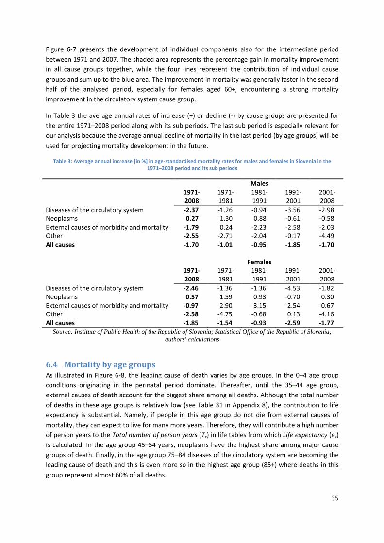
35

Figure 6-7 presents the development of individual components also for the intermediate period

between 1971 and 2007. The shaded area represents the percentage gain in mortality improvement

in all cause groups together, while the four lines represent the contribution of individual cause

groups and sum up to the blue area. The improvement in mortality was generally faster in the second

half of the analysed period, especially for females aged 60+, encountering a strong mortality

improvement in the circulatory system cause group.

In Table 3 the average annual rates of increase (+) or decline (-) by cause groups are presented for

the entire 1971–2008 period along with its sub periods. The last sub period is especially relevant for

our analysis because the average annual decline of mortality in the last period (by age groups) will be

used for projecting mortality development in the future.

Table 3: Average annual increase [in %] in age-standardised mortality rates for males and females in Slovenia in the 1971–2008 period and its sub periods

Males 1971-

2008 1971-1981

1981-1991

1991-2001

2001-2008

Diseases of the circulatory system -2.37 -1.26 -0.94 -3.56 -2.98 Neoplasms 0.27 1.30 0.88 -0.61 -0.58 External causes of morbidity and mortality -1.79 0.24 -2.23 -2.58 -2.03 Other -2.55 -2.71 -2.04 -0.17 -4.49 All causes -1.70 -1.01 -0.95 -1.85 -1.70 Females 1971-

2008 1971-1981

1981-1991

1991-2001

2001-2008

Diseases of the circulatory system -2.46 -1.36 -1.36 -4.53 -1.82 Neoplasms 0.57 1.59 0.93 -0.70 0.30 External causes of morbidity and mortality -0.97 2.90 -3.15 -2.54 -0.67 Other -2.58 -4.75 -0.68 0.13 -4.16 All causes -1.85 -1.54 -0.93 -2.59 -1.77

Source: Institute of Public Health of the Republic of Slovenia; Statistical Office of the Republic of Slovenia;


6.4 Mortality by age groups As illustrated in Figure 6-8, the leading cause of death varies by age groups. In the 0–4 age group

conditions originating in the perinatal period dominate. Thereafter, until the 35–44 age group,

external causes of death account for the biggest share among all deaths. Although the total number

of deaths in these age groups is relatively low (see Table 31 in Appendix 8), the contribution to life

expectancy is substantial. Namely, if people in this age group do not die from external causes of

mortality, they can expect to live for many more years. Therefore, they will contribute a high number

of person years to the Total number of person years (Tx) in life tables from which Life expectancy (ex)

is calculated. In the age group 45–54 years, neoplasms have the highest share among major cause

groups of death. Finally, in the age group 75–84 diseases of the circulatory system are becoming the

leading cause of death and this is even more so in the highest age group (85+) where deaths in this

group represent almost 60% of all deaths.

36

Figure 6-8: Age-standardised death rates by cause of death (five main cause groups with the biggest share among total deaths), 2008

0%

10%

20%

30%

40%

50%

60%

70%

80%

90%

100%

0-4

5-1

4

15

-24

25

-34

35

-44

45

-54

55

-64

65

-74

75

-84

85

+

Age groups

Other

Diseases of the musculoskeletal system and connective tissueSymptoms, signs and abnormal clinical and laboratory findings, not elsewhere classifiedDiseases of the circulatory system

Diseases of the skin and subcutaneous tissue

Mental and behavioural disorders


Endocrine, nutritional and metabolic diseases

Neoplasms

Diseases of the genitourinary system



Certain conditions originating in the perinatal period

Certain infectious and parasitic diseases

Diseases of the nervous system


In Appendix 9 the same analysis is presented separately by gender. There are some distinctive

differences between both genders. External causes of death have lower shares among total deaths

for females than males during the entire lifetime. Neoplasms represent considerably higher shares

for females than males in the 25–64 age group, while in the same age diseases of the circulatory

system have higher shares among males than among females. The gender differences by all causes of

death and age groups are presented in Table 34 in Appendix 9.

6.5 Age-specific trends in the top three major cause groups of death Next we analyse trends in mortality by age groups. We only analyse the three main cause groups of

death with the highest shares in 2008, presented in Figure 6-4. The standardisation procedure is not

needed this time.

6.5.1 Diseases of the circulatory system

The decline was not equal for all age groups. In Figure 6-9 we present the decline during the analysed

period by age groups. We compare the central death rate (5mx) from the end of the analysed period

with those from the beginning of the analysed period. Mortality rates decomposed by 5-year age

groups in the Slovenian population of just 2 million are subject to a large random factor, especially in

age groups where mortality is low. To alleviate the random factor, we use 5-year averages at the

beginning and at the end of the analysed period. However, this results in the loss of some dynamics

because the analysed period is somehow shortened by 4 years. The results are presented in the form

37

of indexes. Thus, we present averages of 5mx for 2004–2008 compared to 5mx averages for 1971–

1975.

The biggest decline in mortality for males was in ages from 65 to 84 years – by about 60% – while in

lower age groups it was 50%–55%. In the highest age group (85+), the decline was only about 35%.

Observing the development in time reveals that the result is also affected by increasing mortality in

the 85+ age group in the 1971–1976 period (see Figure 6-10). As discussed, this could be a result of

better identification of causes of death – i.e. relocating cases from the “not elsewhere classified”

category). However, dropping these first 6 years (1971–1976) from the analysis still results in a

smaller mortality decline in this age group compared to the 65–84 age group.

Figure 6-9: Diseases of the circulatory system: level of age-specific mortality rates in 2004–2008 compared to 1971–1975 and 1977–1981 by age groups [indexes]

0

10

20

30

40

50

60

70

40

-44

45

-49

50

-54

55

-59

60

-64

65

-69

70

-74

75

-79

80

-84

85

+

Index, Male (2004-2008)/(1971-1975)

Index, Male (2004-2008)/(1977-1981)

Index, Female (2004-2008)/(1971-1975)

Index, Female (2004-2008)/(1977-1981)



For females the pattern is similar, but much more pronounced. The largest decline in mortality was in

the age group 65–69 – in 2004–2008 it fell to just 20% of the level in 1971–1975. For females in other

age groups the decline was also very strong – to about 30%. However, the exception is the decline in

the 85+ age group, which was modest. Mortality declined by less than one-third – to about 70% of

the 1971–1975 level.

Figure 6-10 and Figure 6-11 present the development of central death rates through time by age

groups. To preserve clarity in these figures we do not present the results for the lowest age groups

because of the small number of cases – note that the scale on the y-axis in these figures is

logarithmic. Because of the small number of cases (about 0–2 cases per 100,000 population in the

last several years), the random effect is large and mortality in these age groups does not have a

substantial impact on total deaths. In any case, the patterns in these age groups are not that

different than the patters in the lowest age groups for which the results are presented in figures.

38

In diseases of the circulatory system cause group of death, the evidence stresses the importance of

reducing the risk factor. In his work, Capewell cites analyses discovering that in Scotland, England and

Wales, Ireland, Finland, New Zealand and the USA about 45%–75% of the decline in mortality related

to this cause can be attributed to changes in risk factors, while only the remaining 25%–55% can be

attributed to treatments (Ridsdale & Gallop, 2010b, p. 24).

Figure 6-10: Diseases of the circulatory system: age-specific mortality rates in 1971–2008 by age groups; males

0.0001

0.001

0.01

0.1

1

19

71

19

73

19

75

19

77

19

79

19

81

19

83

19

85

19

87

19

89

19

91

19

93

19

95

19

97

19

99

20

01

20

03

20

05

20

07

40-44

45-49

50-54

55-59

60-64

65-69

70-74

75-79

80-84

85+


Figure 6-11: Diseases of the circulatory system: age-specific mortality rates in 1971–2008 by age groups; females

0.00001

0.0001

0.001

0.01

0.1

1

19

71

19

73

19

75

19

77

19

79

19

81

19

83

19

85

19

87

19

89

19

91

19

93

19

95

19

97

19

99

20

01

20

03

20

05

20

07

40-44

45-49

50-54

55-59

60-64

65-69

70-74

75-79

80-84

85+


6.5.2 Neoplasms

During the analysed period there was practically no change in central death rates in ages between 50

and 79 in the neoplasms cause group of death (the index is around 100, see Figure 6-12). In lower

39

age groups, there was a substantial decline in mortality, while in the highest age group (85+)

mortality more than doubled. This could be due to an increase in risk factors, but it can also be

suspected that with the strong decline of mortality in diseases of the circulatory system cause group

of death people “hit” this cause group of death instead.

Figure 6-12: Neoplasms: level of age-specific mortality rates in 2004–2008 compared to 1971–1975 by age groups [indexes]

0

50

100

150

200

2502

0-2

4

25

-29

30

-34

35

-39

40

-44

45

-49

50

-54

55

-59

60

-64

65

-69

70

-74

75

-79

80

-84

85

+

Ind

ex

Age group

Index, Male (2004-2008)/(1971-1975)

Index, Female (2004-2008)/(1971-1975)



Figure 6-13: Neoplasms: age-specific mortality rates in 1971–2008 by age groups; males

0.0001

0.001

0.01

0.1

19

71

19

73

19

75

19

77

19

79

19

81

19

83

19

85

19

87

19

89

19

91

19

93

19

95

19

97

19

99

20

01

20

03

20

05

20

07

Log(

mx)

Year

40-44

45-49

50-54

55-59

60-64

65-69

70-74

75-79

80-84

85+


40

Figure 6-14: Neoplasms: age-specific mortality rates in 1971–2008 by age groups [indexes]; females

0.0001

0.001

0.01

0.1

19

71

19

73

19

75

19

77

19

79

19

81

19

83

19

85

19

87

19

89

19

91

19

93

19

95

19

97

19

99

20

01

20

03

20

05

20

07

Log(

mx)

Year

40-44

45-49

50-54

55-59

60-64

65-69

70-74

75-79

80-84

85+


6.5.3 External causes of morbidity and mortality

In this cause group of death the mortality decline for people below age 70 was about 40% – in the

ages of 30s and early 40s, the decline was even about 50% (see Figure 6-15). Above age 70 the

mortality improvement was more modest, while in the highest age group (85+) mortality has not

improved at all.

Figure 6-15: External causes of morbidity and mortality: level of age-specific mortality rates in 2004–2008 compared to 1971–1975 by age groups [indexes]

0

20

40

60

80

100

120

20

-24

25

-29

30

-34

35

-39

40

-44

45

-49

50

-54

55

-59

60

-64

65

-69

70

-74

75

-79

80

-84

85

+

Ind

ex

Age group

Index, Male (2004-2008)/(1971-1975)

Index, Female (2004-2008)/(1971-1975)



41

Figure 6-16: External causes of morbidity and mortality: age-specific mortality rates in 1971–2008 by age groups; males

0.0001

0.001

0.01

0.1

19

71

19

73

19

75

19

77

19

79

19

81

19

83

19

85

19

87

19

89

19

91

19

93

19

95

19

97

19

99

20

01

20

03

20

05

20

07

Log(

mx)

Year

20-24

25-29

30-34

35-39

40-44

45-49

50-54

55-59

60-64

65-69

70-74

75-79

80-84

85+


Again, in Figure 6-16 and Figure 6-17 the mortality development by age groups is presented. Female

mortality differs from male mortality in lower age groups – while female mortality during the

analysed period does not exceed the 0.1% threshold (0.001 threshold in Figure 6-17) up until age 60,

males’ mortality exceeds this threshold already practically in all age groups above the age of 20.

Figure 6-17: External causes of morbidity and mortality: age-specific mortality rates in 1971–2008 by age groups; females

0.0001

0.001

0.01

0.1

19

71

19

73

19

75

19

77

19

79

19

81

19

83

19

85

19

87

19

89

19

91

19

93

19

95

19

97

19

99

20

01

20

03

20

05

20

07

Log(

mx)

Year

20-24

25-29

30-34

35-39

40-44

45-49

50-54

55-59

60-64

65-69

70-74

75-79

80-84

85+


6.6 Age-specific trends in the top three major cause groups of death Based on the past development in mortality by age groups, we present mortality and longevity

projections for the next 50 years. The model assumes a gradual transition from the recently observed

annual rates of mortality improvement into “long-term” rates of mortality improvement that are

arbitrarily determined by the user. A linear transition is assumed. The model results in deterministic

mortality projections. However, we also present a sensitivity analysis for several sets of assumptions.

42

This approach was also used in studies by the research group Continuous Mortality Investigation

(2009a, 2009b).

As mentioned, the model builds on the assumption of an annual improvement (decline) in mortality.

It is gradually converging from initial rates of mortality improvement (annual growth rates) to the

long-term mortality rates – by age groups.

To capture recent development in mortality by age groups we would like to use annual growth rates

of mortality (by age groups) from the last year. However, because of the small number of deaths –

especially in lower age groups – the variability is huge. Therefore, we use the average annual growth

rate by age groups in the 2000–2008 period instead. The variability of mortality growth rates by age

using this approach is still high.

If the average annual growth of mortality rates for the 2000–2008 period is generally below the

average annual growth rate of mortality for the 1971–2008 period and is only above it in one age

group, while in the “neighbour” age groups it is not, we prefer to take a lower value (from the 1971–

2008 time period). Namely, we assume that it is a consequence of the random effect, especially if the

average annual growth of the mortality rate for the 1971–2008 period is similar to the neighbour age

groups. Further, for the 0–24 age groups the average annual mortality rate growth in the entire

1971–2008 period is taken. Due to the small number of death cases in these age groups, the

variability is too high otherwise. The described solutions introduce personal judgement. However, it

does not affect the main results much because the solutions predominately refer to age groups with

low mortality. In any case, the model is based on expert opinions and, therefore, the model is

subjective as such. Actual mortality rates from 2008 are taken as starting values of mortality rates by

age. Results of the projections are presented for various scenarios.

6.6.1 Scenario 1

In Scenario 1 we follow the work of the Continuous Mortality Investigation research group (2009a,

2009b). They assume a 10-year transition period for ages up to 50 and, from age 50 to 60, a gradual

increase in transition period by one year for each consecutive age (from a transition period of 10

years for 50 years of age to a transition period of 20 years for 60 years of age). However, since our

model uses 5-year age groups we use a 12-year transition period for the 50–54 age group and 17

years for the 55–59 age group. From 60 to 80 years a transition period of 20 years is taken. From 80

to 95 a gradual decrease from 20 to a 5-year transition period is assumed, keeping it at a 5-year

transition period thereafter (Continuous Mortality Investigation, 2009a, p. 14). In our model with

5-year age groups we use a transition period of 18 years for the age group 80–84, while for age 85+

we assume a transition period of 13 years.

A 1% long-term rate of mortality improvement is assumed, without a constant addition to rates of

mortality improvement. In Scenario 1 we assume a long-term annual mortality decline of 1% for all

cause groups of death.

Following the described approach we obtain the results presented in Figure 6-18 and Table 4 and

Table 5. A strong decline in mortality rates is projected for the starting years of the projections.

Consequently, life expectancy for all ages is also growing fast in this period, which is in line with the

rapid increase in life expectancy that we have been facing in Slovenia over the last one to two

43

decades. A further improvement in mortality depends on the assumed long-term mortality decline –

which in Scenario 1 is 1%.

Figure 6-18: Annual rate of improvement in mortality [%] and mortality rate of standard population [%] in 2010–2060 projection period, decomposed by cause of death; Scenario 1



We obtained the presented results from central death rates obtained as the sum of central death

rates by four cause groups of death: “diseases of the circulatory system”, “neoplasms”, “external

causes of morbidity and mortality” and “other causes of death”. In Appendix 10 we also present

results for life expectancy by age and gender whereby the rate of mortality improvement is

calculated using the described procedure using the total mortality rate as an aggregate category –

not as the sum of the individual cause groups of death.

0.0

0.5

1.0

1.5

2.0

2.5

2010 2015 2020 2025 2030 2035 2040 2045 2050 2055 2060

An

nu

al r

ate

of i

mp

rove

men

t in

mo

rtal

ity

[%]

Year

Females

Circulatory

Neoplasms

External

All other causes

0

1

2

3

4

5

6

7

8

9

2010 2015 2020 2025 2030 2035 2040 2045 2050 2055 2060

Mo

rtal

iy r

ate

of s

tand

ard

popu

lati

on [

%],

de

com

pose

d by

cau

se o

f de

ath

Year

Females

Circulatory

Neoplasms

External

All other causes

0.0

0.5

1.0

1.5

2.0

2.5

3.0

2010 2015 2020 2025 2030 2035 2040 2045 2050 2055 2060

An

nu

al r

ate

of i

mp

rove

men

t in

mo

rtal

ity

[%]

Year

Males

Circulatory

Neoplasms

External

All other causes

0

1

2

3

4

5

6

7

8

9

2010 2015 2020 2025 2030 2035 2040 2045 2050 2055 2060

Mo

rtal

iy r

ate

of s

tand

ard

popu

lati

on [

%],

de

com

pose

d by

cau

se o

f de

ath

Year

Males

Circulatory

Neoplasms

External

All other causes

44

Table 4: Life expectancy for males, by age; Scenario 1, mortality rates are calculated as the sum of assumed mortality rates by cause groups of death

2010 2015 2020 2025 2030 2035 2040 2045 2050 2055 2060

0 76.31 77.68 78.63 79.38 80.01 80.64 81.27 81.92 82.58 83.25 83.94 1–4 75.51 76.84 77.79 78.53 79.15 79.77 80.40 81.04 81.70 82.37 83.05 5–9 71.57 72.90 73.84 74.58 75.20 75.82 76.45 77.09 77.74 78.41 79.09 10–14 66.58 67.90 68.85 69.59 70.21 70.83 71.45 72.09 72.74 73.41 74.09 15–19 61.63 62.95 63.90 64.63 65.25 65.87 66.49 67.13 67.78 68.45 69.13 20–24 56.82 58.13 59.06 59.79 60.41 61.02 61.63 62.27 62.91 63.57 64.25 25–29 52.04 53.33 54.26 54.98 55.59 56.19 56.80 57.43 58.07 58.72 59.39 30–34 47.22 48.50 49.42 50.14 50.74 51.33 51.94 52.56 53.19 53.84 54.51 35–39 42.39 43.66 44.57 45.28 45.88 46.47 47.07 47.69 48.32 48.96 49.62 40–44 37.64 38.88 39.79 40.49 41.08 41.66 42.26 42.87 43.49 44.13 44.78 45–49 33.02 34.24 35.14 35.83 36.41 36.98 37.56 38.16 38.77 39.40 40.05 50–54 28.64 29.81 30.69 31.37 31.93 32.48 33.05 33.63 34.23 34.84 35.48 55–59 24.44 25.57 26.43 27.09 27.62 28.15 28.70 29.26 29.84 30.43 31.05 60–64 20.62 21.69 22.50 23.13 23.63 24.14 24.65 25.19 25.74 26.31 26.89 65–69 16.92 17.90 18.65 19.23 19.70 20.18 20.67 21.17 21.70 22.24 22.80 70–74 13.34 14.12 14.74 15.25 15.69 16.14 16.61 17.09 17.59 18.12 18.66 75–79 10.32 10.94 11.45 11.89 12.29 12.71 13.15 13.60 14.07 14.57 15.09 80–84 7.69 8.15 8.55 8.92 9.29 9.68 10.09 10.52 10.97 11.44 11.94

85+ 5.85 6.23 6.58 6.92 7.28 7.65 8.05 8.46 8.90 9.36 9.84 Source: Institute of Public Health of the Republic of Slovenia, Statistical Office of the Republic of Slovenia;


Table 5: Life expectancy for females, by age; Scenario 1, mortality rates are calculated as the sum of assumed mortality rates by cause groups of death

2010 2015 2020 2025 2030 2035 2040 2045 2050 2055 2060 0 83.06 84.06 84.83 85.47 86.07 86.67 87.29 87.93 88.58 89.26 89.97 1–4 82.24 83.24 84.00 84.64 85.22 85.82 86.43 87.06 87.72 88.39 89.09 5–9 78.26 79.26 80.01 80.65 81.24 81.83 82.45 83.08 83.73 84.40 85.10 10–14 73.33 74.33 75.08 75.72 76.30 76.89 77.50 78.13 78.78 79.45 80.15 15–19 68.36 69.36 70.11 70.74 71.33 71.92 72.53 73.16 73.80 74.47 75.17 20–24 63.43 64.43 65.17 65.81 66.39 66.97 67.58 68.21 68.85 69.52 70.21 25–29 58.48 59.47 60.22 60.85 61.42 62.01 62.62 63.24 63.89 64.55 65.24 30–34 53.56 54.54 55.28 55.91 56.49 57.07 57.67 58.30 58.94 59.60 60.29 35–39 48.65 49.62 50.36 50.99 51.56 52.14 52.74 53.36 54.00 54.66 55.35 40–44 43.75 44.72 45.45 46.07 46.64 47.22 47.82 48.44 49.07 49.73 50.42 45–49 38.93 39.87 40.60 41.22 41.78 42.36 42.95 43.56 44.19 44.85 45.53 50–54 34.18 35.09 35.81 36.42 36.98 37.55 38.13 38.74 39.37 40.01 40.69 55–59 29.68 30.57 31.27 31.86 32.41 32.96 33.53 34.12 34.74 35.38 36.04 60–64 25.20 26.06 26.74 27.32 27.84 28.38 28.94 29.52 30.12 30.75 31.40 65–69 20.87 21.67 22.32 22.87 23.38 23.90 24.44 25.01 25.60 26.21 26.85 70–74 16.69 17.41 18.00 18.52 19.01 19.52 20.05 20.60 21.17 21.77 22.39 75–79 12.84 13.46 13.99 14.47 14.94 15.43 15.94 16.47 17.02 17.61 18.22 80–84 9.55 10.08 10.55 10.98 11.43 11.89 12.38 12.89 13.43 13.99 14.58

85+ 7.03 7.51 7.92 8.33 8.76 9.21 9.69 10.19 10.71 11.26 11.84 Source: Institute of Public Health of the Republic of Slovenia, Statistical Office of the Republic of Slovenia;


45

6.6.2 Scenario 2 and Scenario 3

Following the work of the Continuous Mortality Investigation research group (2009a, 2009b), in

Scenario 1 we have a 1% long-term rate of mortality improvement for all cause groups of death. This

(uniform) 1% level of long-term mortality improvement could be the subject of discussion.

For example, in a survey conducted by the Society of Actuaries in 1998, experts from different fields

were asked to provide their best guess for the ultimate annual rate of improvement in mortality

rates beyond the year 2020 for the age group 65+. From a total of 59 experts coming from Canada,

Mexico and the United States, there were 37 actuaries, 9 demographers, 8 economists and 5 from

other professions (Rosenberg & Luckner, 1998, p. 65). For males their mean estimates were 0.58%

(Canadian males), 0.76% (Mexican males) and 0.67% (US males), while for females their estimates

were 0.64% (Canadian females), 0.83% (Mexican females) and 0.70% (US females) (Rosenberg &

Luckner, 1998, p. 75). Thirteen per cent of respondents believed that a method using cause-specific

mortality rates will produce a better forecast than a method projecting aggregate mortality, while 41

of the respondents thought that a cause-specific projection is a good first step for the aggregate

study and 42 (8 of the 9 demographers) agreed it was a useful indicator of the reasonableness of the

projection (Rosenberg & Luckner, 1998, p. 66). In some other projections somewhat lower values

were used, while for some European countries (Germany, Switzerland and Austria) much higher

values were assumed – for most age groups between 1% and 3% per annum (see Continuous

Mortality Investigation, 2009b, p. 55).

In Scenario 2 we will therefore present results assuming a lower long-term rate of mortality

improvement than in Scenario 1 – of 0.5% per annum – while in Scenario 3 we will assume a higher

long-term rate of mortality improvement – of 1.5% per annum. In addition, in Scenario 2 we assume

a higher long-term rate for the neoplasms cause group of death. In particular, we assume a 1.0%

long-term rate of mortality improvement (while for other cause groups of death we assume 0.5%

annual growth). We have already mentioned the rationale for this assumption – low improvements

in the past may be due to decreasing mortality in the “diseases of the circulatory system” cause

group. It might be the case that for people not dying from a circulatory cause of death, people “hit”

the neoplasms cause of death instead, although there might be a substantial improvement in

identifying and curing this disease. Scenarios 2 and 3 are presented in Appendix 11: Figure 11-7 and

Figure 11-8 and Tables 37–40.

The presented results should be regarded with caution. To all the previously mentioned problems

(see Section 6.1) we can also add broadly defined cause of death groups, which can therefore be very

heterogenic. We have to bear in mind that there are complex problems of comorbidity, subsidiary

causes and distinctions between the proximal and underlying causes of death. In older ages people

often have more than one disease interacting with each other, making the identification of each of

them more difficult, and only one of them is identified as a (main) cause of death. Further, there

might be a big time lag between the change in risk factors and their effect on mortality (Ridsdale &

Gallop, 2010b).

6.7 Two lifestyle factors affecting mortality In a report from 2009 the World Health Organisation (WHO) summarises that “the leading global

risks for mortality in the world are high blood pressure (responsible for 13% of deaths globally),

tobacco use (9%), high blood glucose (6%), physical inactivity (6%), and overweight and obesity (5%)”

46

(World Health Organisation, 2009). We will present data available for some of the factors that are

believed to affect mortality. Analysing the trends of these factors can be helpful for preparing

assumptions about the future development of central death rates. The available data for the

Slovenian case are not detailed enough to allow a more advanced analysis of the connections

between these factors and deaths by major cause groups.

6.7.1 Smoking

The decline in tobacco consumption is supposed to be one of the key factors underpinning the

mortality decline seen in diseases of the circulatory system cause group of death during the last few

decades. It is believed that tobacco also contributes to many other causes of death. Tobacco

accounted for 18% of deaths in high-income countries, while for specific cancers its impact is

especially high. It is reported that tobacco smoking alone causes 71% of lung cancer deaths

worldwide (World Health Organisation, 2009, p. V). Peto et al. conducted a study based on surveys in

45 developed countries for the 1950–2000 period. They conclude that smoking is currently

responsible for about two million deaths per year, about half of which are concentrated in ages

between 35 and 69 (Ridsdale & Gallop, 2010b, p. 25).

For the Slovenian case, rich data sets on smokers are not available. However, in the WHO databases

data on “regular daily smokers in the population, age 15+” for some years are available. The data are

presented in Figure 6-19. They show a clear negative trend in the 1988–2007 period. While in 1988

more than one-third of people aged 15+ were regularly smoking, in 2007 this share had dropped to

less than one-fifth. As indicated by the linear trend line, the share of regularly daily smokers was

declining in the 1988–2007 period on average by 0.75 of a percentage point per annum. The trend is

negative for both males and females, but in the 1988–2007 period the trend was more negative for

males than for females and therefore the difference between the two genders decreased.

Figure 6-19: Percentage of regular daily smokers in the population, age 15+

y = -0.7498x + 34.085R² = 0.9485

0

5

10

15

20

25

30

35

40

19

88

19

89

19

90

19

91

19

92

19

93

19

94

19

95

19

96

19

97

19

98

19

99

20

00

20

01

20

02

20

03

20

04

20

05

20

06

20

07

Shar

e [%

]

Year

Both genders

Males

Females

Linear (Both genders)

Source: World Health Organisation

Results for other countries suggest that smoking is closely related to various cause groups of death.

Based on these results, which reveal a strong decline in smoking habits among the Slovenian

47

population, we conclude that smoking is one of the very important factors that also explain the

mortality decline seen in the last few decades in the Slovenian case.

6.7.2 Alcohol

Alcohol consumption is another lifestyle variable for which we have available data. From Figure 6-20,

a substantial decline during the 1981–2005 period can be observed. Alcohol has a negative effect on

people’s health, especially if people drink it in large quantities for a longer period.

Figure 6-20: Alcohol consumption in the 1981–2005 period – total consumption and the consumption by sorts of alcoholic drinks

y = -0.1779x + 13.548R² = 0.5864

0

2

4

6

8

10

12

14

16

18

19

81

19

82

19

83

19

84

19

85

19

86

19

87

19

88

19

89

19

90

19

91

19

92

19

93

19

94

19

95

19

96

19

97

19

98

19

99

20

00

20

01

20

02

20

03

20

04

20

05

Litr

es

pe

r ca

pit

a

Year

Pure alcohol consumption, litres per capitaSpirits consumed in pure alcohol, litres per capitaWine consumed in pure alcohol, litres per capitaBeer consumed in pure alcohol, litres per capitaLinear (Pure alcohol consumption, litres per capita)


In addition, if one drives with alcohol in the blood the probability of causing a traffic accident rises

strongly. In Many other risk factors have an important impact on mortality. For example, we would

like to have data on body mass index, data on the consumption of medications that substantially

reduce mortality for big groups of diseases etc.

Figure 6-21 the number of traffic accidents per 100,000 population is presented. However, the

increasing trend could be misleading because the number of register vehicles and the number of

people driving vehicles has also substantially increased, so data for these aspects should be obtained

for the same period. In addition, time spent in traffic could change. The decomposition of traffic

accidents by cause could be another candidate for appropriately measuring the effect of alcohol on

traffic accidents.

Many other risk factors have an important impact on mortality. For example, we would like to have

data on body mass index, data on the consumption of medications that substantially reduce

mortality for big groups of diseases etc.

48

Figure 6-21: Road traffic accidents involving alcohol per 100,000 population

0

10

20

30

40

50

60

70

80

90

100

19

80

19

82

19

84

19

86

19

88

19

90

19

92

19

94

19

96

19

98

20

00

20

02

20

04

Ro

ad t

raff

ic a

ccid

en

ts in

volv

ing

alco

ho

l pe

r 1

00

00

0 p

op

ula

tio

n

Year


6.8 Conclusions By far the most important causes of death in Slovenia in 2008 were “diseases of the circulatory

system” (39.5% of all deaths) and “neoplasms”, i.e. cancer (31.4% of all deaths). By also including the

third largest group – deaths caused by external causes (8.3% of all deaths) – about 80% of all deaths

are included in the analysis. The trends of these three cause groups of death differ. Diseases of the

circulatory system exhibit a strong decline in the 2071–2008 period: from over 900 to less than 400

deaths per 100,000 population (using a standard population from 2008) in the 1971–2008 period.

Representing a high share among all causes of death, this group is a main driving force in the decline

of total mortality in the 1971–2008 period in Slovenia. Although the share of external causes of

morbidity and mortality is much smaller and the negative trend is less pronounced, they contribute

substantially to the total mortality decline as well. In contrast, neoplasms do not show any clear

trend. If the trends for these two groups of diseases were to continue, neoplasms would become the

no. 1 cause of death in the near future.

By taking into account the trends in mortality by the three main cause of death groups in the past,

we project the future development of longevity. In a baseline scenario we assume gradual

convergence from initial rates of mortality improvement (average annual growth rates in 2001–2008

period) to a 1% long-term rate of mortality improvement. Under these assumptions, life expectancy

at birth for males would increase from 76.3 years in 2010 to 83.9 years in 2060 whereas for females

it would increase from 83.1 years in 2010 to 90.0 years in 2060.

49

7 FORECASTING MORTALITY USING THE LEE-CARTER

METHODOLOGY In this chapter we give the results for all of the three stochastic methods briefly introduced in

Chapter 4. Based on back-testing results we will decide upon the method for projecting future

mortality. In the next subsection we present the results for the Lee-Carter, Poisson log-bilinear and

APC models. First, we outline the results for the Lee-Carter model vs. Poisson log-bilinear model

based on non-smoothed data due to the fact that both models are three-parameter models and are

thus easier to compare graphically/visually, whereas APC is a five-factor model and hence we analyse

the result in a separate subsection. The code for this chapter was entirely programmed in Matlab.

7.1 Stochastic methods implemented in Slovenian mortality data

7.1.1 The Lee-Carter model vs. the Poisson log-bilinear model

In this chapter we present the results of the model introduced in Brouhns et al. 2002. The results of

the model are compared to the results of the Lee-Carter model (as in Lee and Carter 1992). As

mentioned in the previous sections, we use data from the Slovenian Statistical Office on mortality by

age for the period between 1971 and 2008. For the purpose of our analysis we had to manipulate the

data in order to make the computations feasible. Namely, one assumes when using the LC model

that all ( )xm t are larger than 0. In some instances for Slovenia, especially at older ages due to the

small population involved, this is not the case. In addition, due to sampling issues, data for ages

above 85 for the 1971 to 1980 period are relatively unreliable. Thus, we used some of the methods

mentioned in Pitacco et al. (2010) to adjust the data as described in Section 3.5.

Figure 7-1: Beta(x) as a function of age (males): the Poisson vs. the LC model

0 20 40 60 80 100 1200

0.005

0.01

0.015

0.02

0.025

0.03

0.035

age

beta

(x)

male

As one can see from the figure, beta exhibits highly erratic behaviour when using both methods. This

is mainly a consequence of the small population and relatively small number of both exposures and

deaths, which contribute to the relatively higher volatility of estimates than is the case for larger

50

countries. If one compares these results with the results of the LC model obtained from smoothed

data using m-splines (see Appendix 5), one notices that the trend behaviour is similar in both cases

but with much less noise in the case of smoothed data. Looking at the figure, we observe that over

the past 40 years the biggest improvements in mortality were in the age group of minors, especially

new-borns and kids aged between 10 and 14 years. This is also the age group for which the

discrepancy between the LC and Poisson log-bilinear model is largest. In the case of Poisson log-

bilinear, beta is somewhat larger for this age group than the LC method and slightly lower for most of

other age groups. The results in beta indicate similar trends as in other countries, with the largest

improvements in mortality for lower age groups.

Figure 7-2: Alpha as a function of age (males): the Poisson vs. the LC model

0 20 40 60 80 100 120-9

-8

-7

-6

-5

-4

-3

-2

-1

0

age

alp

ha(x

)

male

The results for alpha for both models indicate there are hardly any differences in calculated values.

The only difference is a small discrepancy in the values of alpha for ages between 2 and 10 years.

Overall, the results of both models are similar to those for other countries. Mortality is relatively high

for new-borns and drops considerably for minors. For teenagers and young adults, mortality is

increasing with a noticeable hump (“the testosterone hump”) around the age of 20. After that age,

mortality is slightly decreasing or constant and starts to linearly increase around the age of 30.

Figure 7-3 shows that with both methods kappa decreases substantially over the observed period

(1971–2008). During that time, we have witnessed a continuous improvement in mortality for all age

groups (also see the corresponding figure for beta). Given an average value of beta of around 0.01,

mortality has on average more than halved for the observed period. Of course, some age groups

(such as minors) have observed decreases in mortality far higher than the average, whereas old age

groups have improvements below or well below the average. If we look at the trend for kappa we

can see that with the LC method kappa is almost linearly decreasing, whereas for the Brounhs et al.

method it seems to be increasing at an even higher rate and exhibits a mild curvature.

51

Figure 7-3: Kappa as a function of year (males): the Poisson vs. the LC model

1970 1975 1980 1985 1990 1995 2000 2005 2010-60

-50

-40

-30

-20

-10

0

10

20

30

40

year

kappa(x

)

male

Figure 7-4: Kappa as a function of year (females): the Poisson vs. the LC model

1970 1975 1980 1985 1990 1995 2000 2005 2010-60

-50

-40

-30

-20

-10

0

10

20

30

40

year

kappa(x

)

female

Looking at the results for females, we can see that the trend in kappa is similar as for males. Kappa is

decreasing almost linearly in time with both methods. Again, both methods yield very similar results

with only slight differences in calculated values for some years. Overall, one can conclude that the

results of the two methods are relatively robust in terms of the obtained values of kappa. From the

values of beta we can again conclude that there are no significant differences between the two

methods. Once again the estimates are not as smooth as the estimates based case on the LC method

using smoothed data. This is a consequence of a small population and relatively small number of

both exposures and deaths, which contribute to a higher volatility of estimates as compared to larger

countries. The biggest difference between the two methods occurs for minors and teenagers, with

the Poisson model giving estimates above those obtained with LC; on the other hand, for age groups

52

above 20 LC gives estimates somewhat higher although the estimates obtained with the two

methods are comparable. Looking at Figure 7-6 presenting alpha, one can see that both methods

yield similar results. Differences in values exist primarily for age groups between 15 and 25. In both

cases, mortality drops significantly for minors and rises thereafter. After age 30 the trend is almost

linear (as already observed by Cairns et al. 2006).

Figure 7-5: Beta(x) as a function of age (females): the Poisson vs. the LC model

0 20 40 60 80 100 1200

0.005

0.01

0.015

0.02

0.025

0.03

age

beta

(x)

female

Figure 7-6: Alpha as a function of age (females): the Poisson vs. the LC model

0 20 40 60 80 100 120-10

-9

-8

-7

-6

-5

-4

-3

-2

-1

0

age

alp

ha(x

)

female

53

7.1.2 The APC model

In the next section we give the results of the APC model for raw (non-smoothed) data for both males

and females. We start with males first.

Figure 7-7: Alpha as a function of age (males): the APC model

0 20 40 60 80 100 120-9

-8

-7

-6

-5

-4

-3

-2

-1

0

age

alp

ha

male

As one can see from Figure 7-7, the values for alpha are similar to the values obtained with other

methods such as the Poisson model (Brouhns et al. 2002) and the simple Lee-Carter model. The

dynamics of beta (see Figure 7-8) are also similar to the Lee-Carter case, with the largest values

occurring at young ages and the lowest values for old ages. There are occasional downward spikes in

beta such as a spike at age 20 and another one around the age of 50, but on average the

improvements in mortality over time have favoured younger generations more than older

generations. Looking at kappa (see Figure 7-9), we observe a similar downward trend as noticed in

the Poisson model and LC model. As shown by the graph, the trend is almost linear and significantly

negative which indicates that the improvements in mortality were significant in the 1971 to 2008

period. Examining the cohort effect given by iota (see Figure 7-10) as a function of birth year, we can

see that the overall effect for cohorts born after 1900 (males) is relatively small. If we compare the

values of iota for Slovenia with the values of iota for the UK (there is also around 40 years of data

with age groups divided between one-year classes from zero to 99 years), we can see that in the

Slovenian case they amount to less than one-tenth of the values for the UK. This indicates that,

compared to the UK, the cohort effect is not as significant. Given this fact when calculating future

mortality, one is led to assume that the differences in projected mortality using the APC, LC or

Poisson models are not significant.

54

Figure 7-8: Beta as a function of age (males): the APC model

0 20 40 60 80 100 120-0.005

0

0.005

0.01

0.015

0.02

0.025

0.03

0.035

age

beta

male

Figure 7-9: Kappa as a function of year (males): the APC model

1970 1975 1980 1985 1990 1995 2000 2005 2010-50

-40

-30

-20

-10

0

10

20

30

40

year

kappa

male

Looking at the values for alpha again, we can conclude that there are no significant differences

among all three models. The dynamics of beta for females are quite different than for males,

especially for teenagers where the effect of the improvement in mortality over time caused only a

mild improvement in mortality. A similar result is observed for the LC model, although the spike

(downward) is not as significant as with the APC model. Observing the values of kappa, we can see

that the trend is again negative and significant with only a mild curvature. By contrast, the cohort

effect is not as straightforward as is the case for males since the 1972 cohort has a significant and

55

negative value of iota. When examining this effect, we do not find any reasonable explanation except

that there might be a problem with the data. We also observe high and highly volatile values of iota

for cohorts born before 1905, which is simply a consequence of the small population size and

probably also the scarcity of data (high age groups with a relatively small exposure and relatively few

deaths).

Figure 7-10: The cohort effect (males): the APC model

1860 1880 1900 1920 1940 1960 1980 2000 2020-30

-25

-20

-15

-10

-5

0

5

10

15male

Figure 7-11: Beta0(x) as a function of age (males): the APC model

0 20 40 60 80 100 120-0.06

-0.04

-0.02

0

0.02

0.04

0.06

0.08

0.1

age

beta

U

male

56

Let us now consider the case of the APC model’s results for females.

Figure 7-12: Alpha(x) as a function of age (females): the APC model

0 20 40 60 80 100 120-9

-8

-7

-6

-5

-4

-3

-2

-1

0

age

alp

ha(x

)

female

Figure 7-13: Beta(x) as a function of age (females): the APC model

0 20 40 60 80 100 1200

0.005

0.01

0.015

0.02

0.025

0.03

age

beta

(x)

female

57

Figure 7-14: Beta0(x) as a function of age (females): the APC model

0 20 40 60 80 100 120-0.04

-0.02

0

0.02

0.04

0.06

0.08

0.1

0.12

0.14

age

beta

U(x

)

female

Figure 7-15: Kappa(t) as a function of year (females): the APC model

1970 1975 1980 1985 1990 1995 2000 2005 2010-50

-40

-30

-20

-10

0

10

20

30

40

year

kappa

female

58

Figure 7-16: The cohort effect (females): the APC model

1860 1880 1900 1920 1940 1960 1980 2000 2020-20

-15

-10

-5

0

5

10

15

20female

7.2 Modelling kappa In order to obtain estimates of future mortality one needs to estimate the dynamics of kappa for

both men and women. As noted by several authors, t can be regarded as a stochastic process that

can be modelled by fitting an ARIMA (p, d, q) model.

7.2.1 Modelling kappa using the Poisson log bilinear model

Now let us look first at the results of the Poisson model (Brouhns et al. 2002). In this case, the value

of c is equal to -2.43 (equation (4.27)). In order to check the validity of the model we have to

examine the statistical properties of the residuals.

Table 6: Summary statistics for residuals using Poisson model (males)

Mean 2.88E-16

Median -0.307543

Maximum 6.586123

Minimum -7.556903

Std. Dev. 3.349367

Skewness -0.049737

Kurtosis 2.642194

Jarque-Bera 0.212627

Probability 0.899143

Sum 1.95E-14

Sum Sq. Dev. 403.8574

No. of observations 37

Source: SORS and own work

Table 6 shows we cannot reject the hypothesis of normally distributed residuals. Both the Jarqure Berra test and the value of the kurtosis and skewness indicate that the normal distribution is a good approximation for the distribution of the residuals. Further, when looking at Q-statistics (see

59

Appendix 4) for autocorrelation we observe that there is no statistically significant autocorrelation.

Figure 7-17: Kappa(t) as a function of time (males): the APC model

1960 1980 2000 2020 2040 2060 2080 2100-350

-300

-250

-200

-150

-100

-50

0

50

year

kappa(t

)

scenarios male

Figure 7-17 reveals quite a strong downward trend in mortality. For the low mortality scenario the

trend is somewhat higher due to the higher than expected decrease in kappa. Likewise for the high

mortality scenario, the decrease in kappa is somewhat lower. We can see that in both cases the

trend is negative, meaning that the reduction in kappa is highly statistically significant.

Now let us consider the result for females. Again the ARIMA (0,1,0) proves to be an adequate model

for modelling the dynamics of kappa.

Table 7: Summary statistics for residuals using the Poisson log bilinear model

Mean -3.24E-16

Median 0.199426

Maximum 6.081238

Minimum -6.402445

Std. Dev. 3.093559

Skewness -0.028232

Kurtosis 2.224110



Sum -7.99E-15

Sum Sq. Dev. 344.5238



60

Figure 7-18: Kappa(t) as a function of time (females): the APC model

1960 1980 2000 2020 2040 2060 2080 2100-300

-250

-200

-150

-100

-50

0

50

year

kappa(t

)

scenarios female

As one may see from Table 7 and the corresponding table in, the residuals obtained using the ARIMA

(0,1,0) model are uncorrelated and approximately normally distributed. Figure 7-18 shows that the

difference between scenarios is increasing in time but the estimates still remain fairly close.

7.2.2 Modelling kappa using the LC model

Now we consider the case of modelling kappa when using the original Lee-Carter model for males.

Again we can see that the simple ARIMA (0,1,0) does a good job of capturing the dynamics of kappa.

The residuals are not autocorrelated, whereas the skewness, kurtosis and Jarqure Berra tests indicate

that the hypothesis of normally distributed residuals cannot be rejected. Another important

consequence of the residual test is the fact that with the LC model the standard deviation of

residuals is higher than with the Poisson log bilinear model. Thus the difference between the

forecasts under the three scenarios is much smaller in the case of the Poisson log bilinear model.

Figure 7-19 reveals there is again quite a strong downward trend in mortality. The trend is somewhat

lower than for the case of the Poisson model but, on the other hand, the standard deviation of

residuals is higher than with the Poisson model. The values for kappa under the high mortality

scenario are thus higher in the original LC model than in the Poisson model. The same goes for the

middle scenario. The values for the low mortality scenario in the LC model are comparable to the

values in the Poisson model.

Now we consider the LC model for females and try to estimate the dynamics of kappa. In contrast to

the case for males, in the case of females the dynamics cannot be modelled as an ARIMA (0,1,0)

model, but can best be fitted by an ARMA(2,2) model. In this case, as one can see from Table 9, the

residuals are not autocorrelated (at least up to the relevant number of lags) and the residuals can be

assumed to be normally distributed.

61

Table 8. Summary statistics for residuals using the LC model (males)

Mean -5.96E-16

Median -3.33E-15

Maximum 10.12461

Minimum -11.78582

Std. Dev. 4.889802

Skewness -0.409455

Kurtosis 3.041657



Sum -2.13E-14

Sum Sq. Dev. 860.7658



Figure 7-19: Projecting kappa using the LC model for the 2008–2088 period (males)

1960 1980 2000 2020 2040 2060 2080 2100-350

-300

-250

-200

-150

-100

-50

0

50

year

kappa(t

)

scenarios maleLC

Table 9. Summary statistics for residuals using the LC model (females)

Mean -0.052288

Median 0.183130

Maximum 7.569289

Minimum -11.08728

Std. Dev. 4.813961

Skewness -0.559959

Kurtosis 2.718712



Sum -1.882381

Sum Sq. Dev. 811.0976



62

Once again, we observe that the standard deviation of estimates of kappa is significantly higher than

with the case of the Poisson log bilinear model. This is again another argument in favour of using

Poisson log-bilinear for modelling future mortality. Namely, with the Poisson log bilinear model the

confidence interval of estimates is much narrower than with the LC and APC models.

7.2.3 Modelling kappa using the APC model

In contrast to the LC and Poisson log bilinear models, the APC model does not allow us to use ARIMA

(0,1,0) to model the evolution of kappa. As one can see, the appropriate model is achieved by using

the AR(2) model, which gives us both uncorrelated residuals that are approximately normally

distributed.

Table 10 demonstrates that the standard error of the kappa model is much higher than with the

Poisson log bilinear model, hence there is a much larger deviance among the three scenarios.

Table 10: Summary statistics for residuals using the APC model (males)

Mean -3.36E-10

Median 0.790038

Maximum 7.113411

Minimum -14.58855

Std. Dev. 5.188256

Skewness -0.785145

Kurtosis 3.209650



Sum -1.21E-08

Sum Sq. Dev. 942.1301



In the case of the APC model (females) we obtain a good fit using the ARMA(1,1,0) model. In this

case, the residuals are again uncorrelated (see Appendix 4).

It is apparent when looking at Table 11 that we cannot reject the hypothesis of normally distributed

residuals. Looking at the standard deviation of the estimates of the kappa model, we see that the

values are again higher than in the case of the Poisson log bilinear model.

63

Table 11: Summary statistics for residuals using the APC model (females)

Mean 1.09E-08

Median 0.122306

Maximum 6.732146

Minimum -9.420403

Std. Dev. 4.217108

Skewness -0.440758

Kurtosis 2.614452



Sum 3.92E-07

Sum Sq. Dev. 622.4401



7.3 Back-testing When making future projections we need to make a quantitative assessment of all three models. This

cannot, of course, be done graphically, so we use the back-testing technique to determine which

model would be most appropriate for estimating future mortality. More precisely, the models

considered are tested against real data (in our case the number of deaths) for the period 2001 to

2008. In the first step, we fit the model parameters to the data for the period 1971 to 2000. In the

second step, the values of the parameters obtained in step one are used to predict the number of

deaths Dxt for the 2001–2008 period. Several quantities of fit measures are then used to compare the

methods.

Table 12. Comparison of methods using back-testing for the 2001–2008 period (males)

LC APC Brouhns

MSE 21 25 20.8

MPE 11.7 13.6 11.6

R^2 0.955 0.935 0.96


Let us first examine the results for males for the period 2001 to 2008. As mentioned, we consider the

number of deaths as a function of age and year as an explanatory variable. As Table 12 shows, the LC

method is, according to all criteria, second best and comes very close to the Poisson log-bilinear

method. On the other hand, according to all measures, APC is clearly last. The supremacy of the

Poisson log-bilinear method is even more convincing in the case of females. Ninety-nine per cent of

all variation in the number of deaths for the period 2001 to 2008 can be explained via this method

(see Table 13).

Table 13. Comparison of methods using back-testing for the 2001–2008 period (females)

LC APC Brouhns

MSE 18.5 25.1 11.5

MPE 11.2 24.9 7

R^2 0.975 0.93 0.99


64

Based on the back-testing analysis, we may conclude that the Poisson log bilinear model best fits the

actual central death rates and will, therefore, use this model for forecasting in the future.

7.4 Expected future lifetime at age 65 by period and population annuity

factor Next we examine the effects of increased longevity on annuities by looking initially at expected

lifetime at age 65 65e and later the immediate pension annuity factor at age 65 65a .

Figure 7-20: The expected remaining lifetime as a function of time for males (using projections for kappa obtained by the Poisson log-bilinear method) by period

1960 1980 2000 2020 2040 2060 2080 210012

14

16

18

20

22

24

26males

year

e65

Looking first at the expected remaining lifetime at 65, we can see that there is a clear upward trend

for males. Over a period of 80 years the expected remaining lifetime at age 65 is expected to further

increase by 8.5 years. If we translate this prolongation of lifetime into monetary units, the increase in

longevity translates into an increase of approximately 21%. The pension annuity factor is expected to

rise from approximately 9.3 to a little less than 11.3.

65

Figure 7-21: The immediate annuity factor as a function of time for males (using projections for kappa obtained by the Poisson log-bilinear method) by period

1960 1980 2000 2020 2040 2060 2080 21007.5

8

8.5

9

9.5

10

10.5

11

11.5males

year

a65

Figure 7-22: The expected remaining lifetime as a function of time for females (using projections for kappa obtained by the Poisson log-bilinear by period

1960 1980 2000 2020 2040 2060 2080 210015

20

25

30females

year

e65

If we consider the case of females, the expected remaining lifetime at age 65 is expected to rise by

approximately an equal number of years as with the case for males (approximately seven years).

Similarly, we can also observe that the immediate annuity factor is expected to increase by 16%.

66

Figure 7-23: The immediate annuity factor as a function of time for females (using projections for kappa obtained by the Poisson log-bilinear method) by period

1960 1980 2000 2020 2040 2060 2080 21008.5

9

9.5

10

10.5

11

11.5

12females

year

a65

8 CONSTRUCTION OF A SLOVENIAN ANNUITY LIFE TABLE To calculate the present value of a future obligation arising from life annuity payments, actuaries

must develop a life table. A life table shows for each age the probability that a person of that age will

die before his or her next birthday. This chapter explains the method used to derive the first

Slovenian annuity tables.

8.1 Life tables In a period life table, life expectancy estimates correspond to age-specific mortality rates at age x

and older ages observed in a given calendar year. In a cohort life table, life expectancy estimates

correspond to age-specific mortality rates at age x and older ages observed for a birth cohort during

a long calendar period.

To construct a life table we must first convert central death rates ( )xm t into probabilities of death,

( )xq t . Let xf be the average number of years lived within the age interval [x, x +1) for people dying

at that age. We follow Renshaw and Haberman (2003a) and assume

10

2

0.15 0,

0.16 0,

x

x

f x male

x female

(8.1)

67

We calculate from the following equation using the piecewise constant forces of mortality

assumption

( )

( )1 ( )

xx

x x

m tq t

f m t

(8.2)

To complete the period life table calculation we follow the methodology described on the Human

Life Table Database webpage. For the period life table we calculate ( )xl t number of survivals and

( )xd t number of deaths by age at period t as

1( ) (1 ( )) ( )

( ) ( ) ( )

x x x

x x x

l t q t l t

d t q t l t

(8.3)

We denote the number of person-years lived within the elementary age interval [x,x+1) with ( )xL t ,

number of person years lived after the exact age x with ( )xT t and life expectancy at exact age

x with ( )xe t . The formula for period life expectancy is as follows:

1

( )1

( )( ) 2

x

x k

kx

x

l t

e tl t

(8.4)

The calculation of the other life table function is shown below:

1

1( ) ( ( ) ( ))

2

( ) ( ) ( )

x x x

x x x

L t l t l t

T t l t e t

(8.5)

To calculate the age cohort life table we must first choose the base cohort birth year . We then

calculate the life table to take diagonal probabilities from birth year as follows

1( ) (1 ( )) ( )

( ) ( ) ( )

x x x

x x x

l q x l

d q x l

(8.6)

Life expectancy is then calculated from

1

( )1

( )( ) 2

x

x k

kx

x

l

el

(8.7)

We can calculate an annuity of size 1 which is payable yearly at the beginning of each year while an

insured is alive from

68

1

0

0

1, 0

( ) (1 )(1 ( ), 0

xkk

x

x jk

j

k

a iq x j k

(8.8)

8.2 Data used for the cohort projections To build the cohort projected life table we first construct the following period tables:

from 1945 to 1970 – the log linear interpolation explained in Section 3.5

from 1971 to 2008 – observed central death rates (see Section 3.5.1)

from 2009 to 2118 – projected with the Poisson log-bilinear method – a point estimate is used

from 2118 – no change in mortality beyond 2118

In this way, we obtain a two-dimensional ( )xm t table, where 0 100x and 1945 2118t .

8.3 Age shifting In this section the approximation method, which leads the calculation for Slovenian population

cohort life tables back to a one-dimensional table, will be explained.

An annuity calculated with a cohort life table not only depends on age at entry, but also on the

individual birth year of the insured person. This would lead to the construction of a cohort life table

for every generation, in turn involving the use of a large series of tables. This is, of course, impractical

and cannot be used in everyday actuarial calculations.

That is why a simplified solution used by several European countries, the so-called Rueff method, has

been adopted. The first cohort period is chosen among a series of generation tables, which we call a

fundamental (or select) cohort. By shifting the actual age, depending on the birth year, the exact

actuarial values will be approximated by using the fundamental cohort with an age shift.

In this respect, the insured persons with birth years above than the birth year of the fundamental

cohort will be made younger, while those with birth years below the birth year of the fundamental

cohort will be made older to account for the trend of the mortality improvement.

Let us denote the chosen fundamental cohort year. Then the adjustment involves an age shift

( )h years (plus or minus). Assuming that mortality declines over time, the function ( )h must

satisfy the following relations:

0,

( ) 0,

0,

h

(8.9)

To determine age shifts ( )h , a criterion is needed that is clearly based on the “differences” or

“distances” between “values” correctly calculated with the intention to use appropriate cohort table

69

and values calculated with the fundamental cohort table.

As regards the type of criteria, usually the expected present value of a life annuity is used. When a

criterion of this type is adopted, function ( )h depends on the interest rate used in calculating the

actuarial values. This is the approach employed by Germany for the construction of life tables. In the

German case, ( )xa is the present value benefit of a life annuity with an annual payment and a

discount rate of 2.75% according to the generation table DAV 2004. In practice, a 2.75% interest rate

could be problematic if we want to calculate expected present values with a rate very far from

2.75%.

If we take 0%, the expected present values coincide with the expected remaining lifetimes (say, at

age 65). Since we want to calculate age shifts appropriate to the Slovenian projected tables, we will

use a combination of both 0% (focusing on the expected lifetime) and the rate used in Slovenia for

pricing and/or reserving for life annuities (currently 2.75%).

We took the following steps to determine ( )h :

For each birth year 1955,.., 2020 and for all ages min maxx x x , where min 55x

and max 65x , the integer shift ( , )ih x is determined, which satisfies the following condition:

( , ) 1 ( , )

( ) ( ) ( )i i

i i i

xx h x x h xa a a

(8.10)

We calculated an annuity with both a 2.75% interest rate and a 0% interest rate (i.e.

(2.75%,0%)i ).

The birth year =1965 was used as the fundamental cohort year because 1965, meaning those who

turned 45 in 2010, is an age that can be considered intermediate between those who enter into a

deferred annuity and insured persons who buy an immediate annuity. This choice will surely produce

an error, which would be reasonably small by using the proposed parameters. The error will increase

with the distance of the actual birth year from the fundamental cohort year.

For each period we obtain a set of ( , )ih x and we choose to select the average value of them to

obtain a single value:

max

min

2.75 2.75

max min

1( ) ( , )

1

x

x x

h h xx x

(8.11)

max

min

0 0

max min

1( ) ( , )

1

x

x x

h h xx x

(8.12)

and

70

2.75 0( ) ( )

( )2

h hh

(8.13)

This age shift ( )h now depends only on the birth year. The resulting age shifts were rounded up to

full years. The result of the procedure is shown in Appendix 2.

8.4 Slovenian reference population mortality table The birth year =1965 was used for the fundamental cohort year to generate a Slovenian base

cohort population mortality table. We then used a smoothing procedure to obtain less variability in

the data. At old ages we used the same procedure as in Section 3.3 for smoothing at very old ages,

with the start smoothing age at 95. Then we smooth the overall data with m-splines with the limit

age at 120. The age cohort life table based on the birth year 1965 is denoted SCO65 (reference

population mortality table) and shown in Appendix 1. Figure 8-1 below shows reference population

mortality rates for males and females (smoothed rates) and non-smoothed rates.

Figure 8-1 Population fundamental mortality rates

0 20 40 60 80 100

-8-6

-4-2

0

1965 Cohort male - smoothed

Age

Log d

eath

rate

0 20 40 60 80 100

-8-6

-4-2

0

1965 Cohort female - smoothed

Age

Log d

eath

rate

0 20 40 60 80 100

-8-6

-4-2

1965 Cohort male - raw

Age

Log d

eath

rate

0 20 40 60 80 100

-8-6

-4-2

1965 Cohort female - raw

Age

Log d

eath

rate

71

8.5 Selection – theoretical background The standardised mortality ratio (SMR) is used as an index for comparing mortality experiences:

actual deaths in a particular population (for example, annuity owners) are compared with those that

would be expected if “standard” age-specific rates were to be applied. The SMR is defined as (Pitacco

et al. 2009)

tan

ˆ ( )

ˆ ( )

xt x

s d

xt x

ETR m t

SMRETR m t

(8.14)

According to Pitacco et al. (2009), SMRs are around 50% for individual and group life insurance

contracts before retirement age, and then decrease to reach 40% for individual policies and increase

to 80% for group life policies for the Belgian population.

A life annuity purchaser is, with a high probability, a healthy person with a particularly low mortality

in the first years of the life annuity payment and, generally, with an expected lifetime higher than

average. In order to take selection into account, Delwarde et al. (2004) suggested a method for

adjusting a reference life table to the experience of a given portfolio, based on non-linear regression

models using local likelihood for inference.

Let us denote ( )HMD

xm t population death rates and ( )LIM

xm t life insurance market rates, then we

define

ln ( ) (ln ( ))LIM HMD

x x xtm t f m t (8.15)

where xt is Normally distributed with a mean 0 and a variance of 2 and ()f is an unknown

smooth function. This model explains the link between population death rates and insurance market

mortality. In Pitacco et al. (2009), the following model is suggested for ages above 60 years:

ln ( ) ( ) ln ( )LIM HMD

x x xtm t f x m t (8.16)

This leads us to produce SMR in the form ˆ ( )f xe , which can be used to adopt mortality projections to

the insurance market. This approach will also be used to estimate Slovenian life insurance market

rates.

8.6 The UK approach to building an insurance annuity table

8.6.1 Methodology

To build “00” Series tables, Continuous Mortality Investigation (CMI) used graduations of GM(r,s)

class of models (the so-called Gompertz-Makeham class of models) in the form

1 1

1 1

expr s

i j

x i j

i j

x x

(8.17)

72

They choose parameters by maximum likelihood, also taking account of the usual diagnostic tests

(numbers of positive and negative deviations, runs, Kolmogorov-Smirnov, serial correlations and 2 ).

At the oldest ages, the values of x for x a , were blended into an arbitrary 120 1 using the

formula:

120

120 120(1 )

120 120

c c

x ac c

x x

a a

(8.18)

A CMI investigation covers data of immediate annuitants, retirement annuitants, personal

pensioners, life office pensioners and widows of life office pensioners.

8.6.2 Observed data

“Immediate annuitants” cover (non-pension) purchased life annuities and they are among the longer

running CMI mortality investigations. It consists of over 64,000 observed males and 142,000

observed females in the period from 1979 to 2002. This investigation is important because it

measures the second type of the selection of immediate annuitants. Tables are published in the “I”

series of life tables.

Table 14: Summary of immediate annuitant tables

Table name Sex Select period Age range

IML00 male None 60 – 120

IFL00 female 1 year 60 – 120

“Retirement annuitants” cover the mortality experience of the self-employed who have purchased

retirement annuities. Data are gathered for both males and females, and are subdivided into two

sections, deferred and vested, which together form the combined section. Tables are published in

the “R” series of the “00” life tables.

“Personal pensioners” represent the mortality experience of holders of personal pension policies

affected under Chapter IV of Part XIV of ICTA 1988. Data are gathered for both males and females,

and are subdivided into two sections, deferred and vested, which together form the combined

section. Tables are published in the “PP” series of the “00” life tables.

“Life office pensioners” cover the mortality experience of life office pensioners, i.e. retirements from

occupational schemes where the benefits have been insured. It is carried out for both sexes on the

basis of both lives and amounts, and is sub-divided into those who retired at or after the normal

retirement age for their scheme (referred to as “Normal” retirements) and those who retired before

their normal retirement age (referred to as “Early” retirements). Tables are published in the “PN”,

“PE” and “PC” series of the “00” life tables. Total numbers of those exposed to risk were around 1.6

million for males and 0.66 million for females (normal lives). Average amounts per life exposed to risk

for 1999–2002 were GBP 2,388.61 for males and GBP 1,272.79 for females (normal lives).

The following GM models were used for the graduation of Normal pensioners’ ultimate experience:

73

Male, Lives : GM(1,4)

Male, Amounts: GM(1,3)

Female, Lives : GM(2,2)

Female, Amounts: GM(2,2)

Table 15: Summary of life office pensioner tables

Table name Category Sex Exposure Age range

PNML00 Normal male Lives 20 – 120

PNMA00 Normal male Amounts 20 – 120

PNFL00 Normal female Lives 20 – 120

PNFA00 Normal female Amounts 20 – 120

PCML00 Combined male Lives 20 – 120

PCMA00 Combined male Amounts 20 – 120

PCFL00 Combined female Lives 20 – 120

PCFA00 Combined female Amounts 20 – 120

PEML00 Early male Lives 50 – 120

PEMA00 Early male Amounts 50 – 120

PEFL00 Early female Lives 50 – 120

PEFA00 Early female Amounts 50 – 120

8.6.3 Projections

It should be pointed out that there are no generally prescribed annuity tables in the UK, so each

company makes its own projections according to the collected data described in the previous

section. Projections are made using the standard exponential formula, the Lee-Carter methodology

and projections with p-splines.

8.7 The German approach to building DAV 2004 R tables

8.7.1 Introduction

The German Actuarial Society (Deutsche Aktuarvereinigung, DAV) came to the conclusion that the

post-2000 DAV 1994 R mortality improvement trend assumption did not appropriately reflect the

mortality improvements in the last three decades of the 20th century. It was decided to develop a

new table, called DAV 2004 R. For the first time it was also assumed that annuitants’ mortality

improvements exceed those of the general population (this is the main basis of their approach).

The DAV 2004 R tables are based on data that encompass 13.7 million years’ exposure from 1995

and 2002. According to the data, the difference between the mortality rates of insured lives and the

general population is slightly more pronounced than was assumed for DAV 1994 R.

The DAV 2004 R table consists of the following components:

• 2nd-order base table: a best estimate of insured lives’ mortality rates in 1999;

• 1st-order base table: the 2nd-order base table reduced to take account of provisions for adverse

deviations;

74

• 2nd-order mortality trend: the best estimate of future mortality improvements; and

• 1st-order mortality trend: the 2nd-order trend increased to take account of provisions for adverse

deviations.

In order to incorporate the selection effect, DAV divided the annuity payment period into six

selection phases by the number of years that have lapsed since the start of the benefit payment: 1st

year,..., 5th year, 6th+ years (“ultimate”).

Selection factors were derived by comparing the mortality rates in the different selection phases

with the population mortality. The figure below shows the various ratios for the observed period.

The initial comment by the working party is that the German selection factors do not differ much

from the UK selection factors.

Figure 8-2 German selection factors

It was assumed that there is an ultimate mortality table for selection phase 6+ and that mortality in

selection phases 1 to 5 is a factor of the ultimate mortality table. This factor depends not on age, but

on gender. There is one factor for selection phase 1 and a common factor for selection phases 2 to 5.

The crude mortality rates for the observed insurance population were first graduated for the age

band 60 to 99 using the weighted Whittaker-Henderson method. The selection factors are then

defined as the ratio of the actual number of deceased persons in the respective selection phase to

the number of deceased persons that would be expected if the graduated ultimate industry mortality

rates were applied to the exposure of insured lives in the respective selection phase.

In this respect, DAV calculated the following selection ratios:

75

Table 16: DAV selection ratios

Males Females

Selection phase 1 0.670538 0.712823

Selection phases 2 to 5 0.876209 0.798230

Outside the age band 60 to 99, DAV extrapolated the ultimate mortality rates. For ages up to 59 they

assume that the ratio of the ultimate mortality rate at age 60 to the 1999 population mortality rate

at age 60 ,1999

pop

xq can be transferred to the younger ages as follows:

6

6

,1999 ,1999

60,1999

66.6%

85.2%

pop popxx x xpop

for menqq q q

for womenq

For older ages, they use a Logistic model for extrapolating the ultimate mortality rates at ages 100 to

120.

8.7.2 Aggregate table for the deferment period

Since the data for deferred annuities did not show a strong selection effect in the deferment period,

the aggregate table was derived for the deferment period, which is not graded in terms of the years

that have lapsed since the commencement date.

In the first step, crude mortality rates were calculated both from the observation material relating to

the deferment period and from the observation material relating to the benefit payment period. The

obtained graduated rates for both data sets are then put together at age 65 in order to obtain

aggregate mortality rates.

8.7.3 Safety margins

The safety margin was applied to face the volatility risk when the table is applied. The idea is to

provide protection against a maximum loss at a defined confidence level. If 1-α=95%, DAV obtains a

margin for volatility risk of 6.26% for males and 7.22% for females. In addition, a 10% flat-rate margin

for level parameter risk is added, meaning that DAV implements a total deduction of 15.6% for males

and 16.5% for females.

8.7.4 Mortality forecasting

For the purpose of forecasting, the traditional exponential formula (see Section 5.3) in the form

, 1

,

exp( ( , ))x t

x t

qF x t

q

(8.19)

was chosen where

76

1 1

1 11 2 1 2

2 1 2 1

2 2

( ), 1999 1999

1999 1999( , ) ( )(1 ) ( ) ,1999 1999

( ), 1999

F x t T

t T t TF x t F x F x T t T

T T T T

F x t T

(8.20)

They calculated age-dependent mortality improvements according to the traditional model

(short-term, long-term and medium-term). In order to compare these trends, the arithmetic means

of annual mortality improvement for ages from 60 to 89 are considered:

Table 17: DAV: Mortality improvement [%]

Males Females

Short-term trend 1.97 2.00

Medium-term trend 1.67 2.05

Long-term trend 0.62 1.04

The so-called initial trend 1( )F x is used for the first years of the mortality projection. This initial

trend is reduced linearly to the target trend in a transition period. The target trend is used after the

transition period. The time 1999 corresponds to the start of the mortality projection.

The loading for insured persons of 0.2% annual mortality improvements is added to the initial trend.

Finally, the trend is extrapolated for high ages to a level of a 1% annual mortality improvement and

limited for low ages to the level of a 3% annual mortality improvement. This defines the initial trend

for insured persons.

The target trend for insured persons was defined as follows: the annual mortality improvement of

the target trend is 75% of the annual mortality improvement of the graduated (and for high ages

extrapolated and for low ages limited) medium-term trend, which was increased by the loading for

insured persons, but not by the medium difference between short- and medium-term trends for

males.

8.7.5 The working party’s comments

The main point when constructing the DAV 2004 R tables was that a loading for insured persons is

needed as an adjustment for differences between the mortality improvement of the population and

the mortality improvement of insured persons. The reason is that private annuities are mainly

purchased by people belonging to upper socio-economic groups, which confirms that the mortality

improvement of annuitants is greater than the mortality improvement of the population (based on

the assumption that the mortality improvement of upper socio-economic groups is greater than the

mortality improvement of lower socio-economic groups).

There is no theoretical justification to assume that the average yearly improvement of mortality for

insured persons is different than the average yearly improvement of mortality for the general

population. It is true that people belonging to upper socio-economic groups mainly purchase private

annuities, and this fact can certainly explain the lower mortality level, in particular at old ages.

However, with regards to improvements, is it reasonable that, starting from lower mortality levels,

77

the socio-economic standard can also justify stronger improvements? If so, the gap between

mortality levels would increase in time. Can we accept this as a reasonable aspect of mortality

trends? We strongly doubt this.

Nevertheless, a reason might be found in the fact that access to new medical and pharmacological

treatments is restricted to high socio-economic classes, and/or that greater awareness of the

benefits of appropriate eating, drinking, smoking etc. habits is also restricted to high socio-economic

classes. If this is the case for Germany, it does not hold for Slovenia and we cannot make projections

on this basis.

In any event, if we accept the “German approach”, then we are implicitly working with

scenario-based projections, which are not “bad” in themselves, but might be more or less

controversial as they imply some judgments and hence some arbitrariness. In contrast with the

scenario-based forecasting used in Section 0 and Section 6, the Lee-Carter methodology allows us to

estimate the lower and upper bounds of the central tendency within a confidence interval.

The working party has some additional remarks regarding the German approach to DAV 2004 R:

1. The selection for observed ages was assumed to stay at the ultimate level, which is not the

case in the UK data. The selection vanished at a very old age since people must eventually die

of something.

2. The parameter risk margin (15%) is added arbitrarily.

3. DAV did not use stochastic methods for mortality forecasting.

4. The scenario-based projections are not in the context of modern mortality frameworks.

8.8 The construction of selection tables for Slovenia

8.8.1 Introduction

Slovenia mortality experience for annuity purchasers is not directly available and because the

pension reform started only 10 years ago, there are no adequate statistical data to make a

conclusion regarding the selection effect. In this respect, we chose an alternative solution introduced

by ANIA (Associazione Natzionale fra la Imprese Assicuratrici, 2005), which was used to build the

Italian insurance annuity tables.

The idea is to use SMR from another population that has similar characteristics as the population

for which we want to introduce the selection effect. As we see from (8.16), SMR in general

depends on age. Let us denote with ( )RC

xSMR t the reference country standardised mortality ratio

for particular year t between the insured and general population. Then we calculate life insurance

market central death rates from

( ) ( ) ( )LIM RC HMD

x x xm t SMR t m t (8.21)

8.8.2 The construction of annuity tables for deferred annuitants for Slovenia

To obtain ( )RC

xSMR t we include an element of selection that emerges from the English data, where

the annuity and pensions market income is, generally speaking, very well developed.

78

We used UK statistical data from 1999–2002 collected by the Continuous Mortality Investigation

Bureau and published in Continuous Mortality Investigation Reports, Number 23 (2009), relating to

the experience of the portfolios of immediate and deferred annuities. The 1999–2002 mortality

investigation presents the so-called “00” Series base mortality tables adopted by the UK Actuarial

Profession. The statistical base is extensive since it involves over 20 million lives exposed to risk.

In particular, we used the mortality investigation of life office pensioners (insured to deferred

annuities) – PNM00 tables for men and PNF00 tables for women, which show the mortality rates for

each age from 20 to 120 years, distinguished between “lives” (heads insured) and “amounts”

(weighted by the benefit).

By comparing the mortality of UK insured lives with that of the general population of the United

Kingdom (taken from English Life Table No. 16, 2000–2002), it was possible to quantify the increased

survival of the insured population. To take account of the influence on the selection of the level of

economic wealth of the insured, as confirmed by the experiences of other markets (for example,

Germany), reference is made to mortality weighted by the size of an annuity.

We calculate:

00

'

16

PNMARCM xx ELT M

x

qSMR

q (8.22)

for males and

00

'

16

PNFARCF xx ELT F

x

qSMR

q (8.23)

for females.

79

Figure 8-3: Selection in the UK population

20 40 60 80 100

0.5

0.6

0.7

0.8

UK Selection

age

Perc

enta

ge

male

female

In Figure 8-3, one can see the huge selection for both men and women from ages 40 to 60.

To correct some irregular patterns and to be closer to the German experience, we chose the

following selection factors of mortality for males and females, respectively:

'

'

'

78

' '

78 78

42,5%, 48

, 48 64

61,5%, 65 71

, 72 77

, 78 107

108(1 ) , 108 120

12

RCM

x

RCM RCMx x

RCM

RCM RCM

x

SMR x

x

SMR SMR x

SMR x

xSMR SMR x

(8.24)

'

'

75

' '

75 75

55%, 50

, 50 75

, 76 111

111(1 ) , 111 120

9

RCF

xRCF

RCFx

RCF RCF

x

SMR x

SMR SMR x

xSMR SMR x

(8.25)

Starting from the cohort life table of generation 1965, which we derived from historical data and

stochastic projections, then applying the selection factors presented in this section, we obtain the

projected and selected mortality table for the generation of insured persons born in 1965. To use the

table for other generations, one should use the age shift tables described in Section 8.3. The

80

complete demographic tables are denoted SDA65.

It must be pointed out that the selection – which is an estimate of the differential mortality of the

insured population which buys annuity insurance from the general population – also depends on the

peculiarities of the products, the characteristics of the insured community to which they relate, and

the business objectives the insurance company intends to pursue.

8.8.3 The construction of aggregate annuity tables for Slovenia

As mentioned in the previous paragraph, SDA65 is structured to represent the mortality of the

insured's deferred annuity or pension insurance. In other cases, such as immediate annuity or

annuity conversion options further selectivity should be added.

In this regard, a comparison was made between mortality relative to insured owners of deferred

annuities with immediate annuitants in the UK – the IML00 and IFL00 tables for men and women,

respectively.

We applied a correction factor to the mortality rates of the SDA65 table for delayed commitments

which includes the increased expected survival of recipients of immediate annuities, namely:

65 65SIA SDA

x x xq q K (8.26)

where

IML00

00

1, 63

, 64 86

1, 87

M xx PNMA

x

x

qK x

q

x

(8.27)

for men and

IFL00

00

1, 54

1 0.02559( 54), 55 59

, 60 84

1, 85

F

x x

PNFA

x

x

x x

K qx

q

x

(8.28)

for women.

We call this life table SIA65. As shown in Section 8.7.2, the mortality of deferred annuitants merges

with the mortality of immediate annuitants after age 60, so SIA65 is a table that may be considered

an aggregate table recommended for use in the annuity business in Slovenia. The tables are

presented in

81

Appendix 3. Selection factors used for aggregate annuity tables are shown in Figure 8-4.

Figure 8-4: Selection factors for aggregate tables

0 20 40 60 80 100 120

0.5

0.6

0.7

0.8

0.9

1.0

Selection factors

Age

sele

ction in %

malesfemales

Figure 8-5: Slovenian gender-related annuity tables

20 40 60 80 100 120

-8-6

-4-2

0

Slovenian annuity tables

age

log r

ate

s

SCO65-female

SCO65-male

SIA65-female

SIA65-male

82

8.8.4 International comparisons

Immediate annuity:

Age at issue 60 / birth year 1950 (annuity starts in 2010)

R94 R04 IPS55 SIA65 SIA65- low mortality scenario

R94/ SIA65

net single premium male

18.104883 20.369429 18.991395 18.50437 18.98097 0.98

net single premium female

20.493777 22.000235 20.705882 20.98405 21.76160 0.97

The net single premium based on SIA65 tables is up to 12% lower than R04 single premium annuities.

The reason for this gap is the 15% margin that is incorporated in the new German tables and the fact

that SIA65 tables represent a best estimate of future annuitant mortality. In this respect those tables

cannot be directly compared. Under the best estimate scenario, we determine future values of

kappa by taking kappa to be equal to the expected value. We also calculated SIA65 under low

mortality scenario. In this case, future values of kappa are obtained by assuming lower than expected

values of kappa. The future values of kappa are obtained by taking 2008 2008 2t ct t . If

we compare low mortality scenario SIA65 single premium with R04, we can observe only marginal

differences in rates (from 1% to up to 7% higher single premium is observed in the case of R04). The

comparisons also show that for current generations who are in front of their retirement, R94 tables

underestimate best estimate annuity from 2% to 4%. We believe that SIA65 should be used for best

estimate valuation of insurance liabilities within Solvency II Framework.



R94/ SIA65


19.720558 22.945504 19.856934 20. 46949

21.28829 0.96


22. 81581 24.426940 21.514670 22. 87369 23.58179 0.97

83



R94/ SIA65


20.87668 24.54484 19.856934 21.5960 22.37775 0.96


24.19244 25.64188 21.514670 23.56325 24.24350 1.03

Deferred annuity

Deferment period 20 years / birth year 1965 / age at issue 45

R94 R04 IPS55 SIA65


9.052749 10.85729 9.573143 9.347653


11.08434 12.00785 10.72477 11.11152

Deferment period 35 years / birth year 1975 / age at issue 35

R94 R04 IPS55 SIA65


5.334621 6.778083 5.486585 5.55777


6.776977 7.600209 6.320382 6.799525

Notation of tables are as follows:

R94 – DAV 1994 R annuity tables

R04 – DAV 2004 R annuity tables

IPS55 – the latest Italian annuity table (2005)

SIA65 – Slovenian aggregate annuity table (2010)

8.9 Unisex annuity tables

8.9.1 Introduction

The European Court of Justice (ECJ) passed new regulation on 1 March 2011 that bans

gender-specific differentiation in insurance pricing. The ECJ ruling means that gender-neutral

premiums and benefits for all new insurance policies taken out after 21 December 2012 should be

84

implemented. This decision will bring important changes to the development of new insurance

products, especially in the life insurance line of business. In this respect, the unisex rates will

introduce new risks of uncertainties arising from the gender mix of the portfolio. This is to a great

extent true for the annuity business where there is still a substantial gap between the life expectancy

of males and females.

An important consequence of the ECJ ruling is that the expected gender mix of an insurance portfolio

will influence product pricing. Since the gender mix can vary significantly for different products,

actuaries should pay special attention when making projections. Among others, the gender mix could

vary depending on the sales channels mix, companies’ orientation to target groups, the employment

ratio of males/females and many more factors.

To be more concrete, when generating unisex annuity tables it is therefore essential that attention is

paid not only to the historical gender-related portfolio mix (i.e. percentage of males and females who

bought an annuity in past), but also to possible future changes of the portfolio arising from the new

market situation. Another consequence of the ECJ ruling will be that the required single premium for

an annuity paid by a female will in most cases be lower. Whether or not this will lead to a situation

whereby the proportion of insured females will increase remains an open question.

Since circumstances are different from company to company, no universal unisex annuity tables can

be recommended. Instead, the methodology will be explained (see the next section) which will lead

to unisex annuity tables.

8.9.2 Unisex annuity tables

In general, we propose two approaches to building unisex annuity tables for Slovenia:

1.

- implement Lee-Carter on the total population

- implement the average (male and female) UK selection factor on Slovenian mortality data

- include an additional selection (gender selection). We can expect that females will more likely buy

annuities since they expect to enjoy annuity payments for a longer time. The question is: How do we

derive the sex selection factor?

2.

- use the already built Slovenian annuity tables for males and females SIA65

- take, as the unisex table, the average of the male table and the female table, with each one having

a weight that should reflect the proportion of males and females, respectively, in future portfolios

(100% would mean that we take female rates)

- calculate age shifts with the same weights

We suggest that actuaries apply approach 2, which uses already built tables. This will give pricing

actuaries flexibility in scenario testing when determining the proper weights for males and females.

We will continue our discussion based on the assumption of approach 2.

A question arising with approach 2 concerns how we can calculate the upper and lower boundaries

of point estimates. In general, lower boundaries of the unisex table cannot be calculated as a

85

weighted average of the male/female lower boundaries since it is a matter of the properties of the

mathematical functions through which the lower boundaries are constructed. If we denote

with L(qM) and L(qF) the lower bounds for probabilities q for males and females, respectively (for a

given age and future year), the weighted average of the lower bounds A(L(qM),L(qF)) is not

necessarily equal to the lower bound of the weighted average L(A(qM,qF)) because A is a linear

function, and the functional form of L is generally not known.

Nevertheless, if we take the lower bounds for males and females as our (prudential) projected

mortality functions, namely if we “forget” that these functions are constructed as lower bounds, the

weighted average clearly represents the average projected mortality function. This approach is

applied whenever a weighted average of elements is used, namely for elements whose construction

is unknown to us.

One more observation: if we take the weighted average of mortality rates, we implicitly assume that

average annuity (in euros) will be the same for males and females.

In Table 18we made a calculation for a unisex single premium for an immediate annuity (birth year

1965), which one can compare with the male and female single premium immediate annuity of the

same cohort. Weights were taken from 45% to up to 65% of the female rates. For example, if w =

45%, then we take 45% of the female rates and 55% of the male rates.

Table 18 Calculation of a unisex single annuity premium

unisex single premium rates

age male female w=45% w=50% w=55% w=60% w=65%

45 24.67695 26.58489 25.536 25.631 25.726 25.822 25.917

50 23.02504 25.14922 23.981 24.087 24.193 24.300 24.406

55 21.22580 23.56325 22.278 22.395 22.511 22.628 22.745

60 19.29927 21.76982 20.411 20.535 20.658 20.782 20.905

65 17.29047 19.71976 18.384 18.505 18.627 18.748 18.870

In the tables below, we calculated the percentage increase of a single premium if unisex rates are

used instead of male rates, and a percentage decrease when female rates are used.

Table 19: Average increase of single premium - male [%]

age w=45% w=50% w=55% w=60% w=65%

45 3.48 3.87 4.25 4.64 5.03

50 4.15 4.61 5.07 5.54 6.00

55 4.96 5.51 6.06 6.61 7.16

60 5.76 6.40 7.04 7.68 8.32

65 6.32 7.02 7.73 8.43 9.13

86

Table 20: Average decrease of single premium – female [%]

age w=45% w=50% w=55% w=60% w=65%

45 -3.95 -3.59 -3.23 -2.87 -2.51

50 -4.65 -4.22 -3.80 -3.38 -2.96

55 -5.46 -4.96 -4.46 -3.97 -3.47

60 -6.24 -5.67 -5.11 -4.54 -3.97

65 -6.78 -6.16 -5.54 -4.93 -4.31

At present, in Italy more than 50% of current annuitants are males. A similar situation is found in

Slovenia, at least for the pension business. In this respect, for a balanced portfolio we suggest taking

unisex rates of around w =60%.

87

9 SUMMARY In 2010 the working group on mortality was established in order to develop the first annuity

mortality tables for the Slovenian market. This document provides a report of the results of the

group’s work.

One of the most important parts of forecasting mortality accurately is to collect appropriate

statistics. The Statistical Office of the Republic of Slovenia (SORS) provided the Slovenian population

data. Data were provided for the time span from 1971 to 2008, for each age and separated for men

and women. Data for the period before 1971 were collected from the Human Mortality Database

(http://www.mortality.org/). Data for mortality by cause analysis were obtained from the Institute of

Public Health of the Republic of Slovenia (IVZ – Inštitut za varovanje zdravja) database for the time

span from 1971 to 2008, for five-year age groups, separately for men and women.

The Slovenian mortality data had some irregularities that needed to be adjusted before we could use

the data for forecasting. We used the method proposed by Denuit and Goderniaux to extrapolate

death rates at very old ages. Following this approach, the death rates for very old ages were

estimated according to the logistic formula. Some death rates were 0 (meaning no deaths in the

observed period), which, due to the small population involved, happens quite often at lower ages.

Since in forecasting we observed log death rates, adjustment techniques were implemented to

obtain positive values. In particular, we used interpolation techniques with neighbour central death

rates to obtain the best estimate for such cases.

General approaches to projecting age-specific mortality rates can be categorised in various ways; for

example, as process-based methods, explanatory methods, forecasting methods or a combination of

these methods.

Forecasting is the process of projecting mortality based on historical trends. Forecasting methods

include some element of subjective judgment, for example, the type of underlying function, the time

series we take into account etc. Simple forecasting methods (for example, exponential formula) are

only usable in the sense that the pattern of changing mortality in the past will continue in the future.

Extrapolation of a time series as an example of forecasting methods assumes that all we need to

know is contained in the historical values of the time series being forecasted. The main shortcoming

of a time-series extrapolation is the assumption that nothing else besides the prior values of a series

is relevant. In this monograph we present two extrapolation methods to project population

mortality. We have adjusted the standard UK exponential formula for forecasting and applied it to

the Slovenian mortality data. The life expectancy derived from the extrapolated mortality data does

not differ from that derived from the LC projections, yet it does not give the prediction interval of the

variability of the prediction.

Explanatory-based methods use econometric techniques based on variables such as economic or

environmental factors. We have employed these techniques to forecast mortality trends by cause.

We have found that by far the most important causes of death in Slovenia in 2008 were “diseases of

the circulatory system” (39.5% of all deaths) and “neoplasms”, i.e. cancer (31.4% of all deaths). By

also including the third largest group – deaths caused by external causes (8.3% of all deaths) – about

http://www.mortality.org/

88

80% of all deaths are included in the analysis. The trends of these three cause groups of death differ.

Diseases of the circulatory system exhibit a strong decline in the 2071–2008 period: from over 900 to

less than 400 deaths per 100,000 population (using a standard population from 2008). Representing

a high share among all causes of death, this group is a main driving force in the decline of total

mortality in the 1971–2008 period in Slovenia. Although the share of external causes of morbidity

and mortality is much smaller and the negative trend is less pronounced, they contribute

substantially to the total mortality decline as well. In contrast, neoplasms do not show any clear

trend. If the trends for these two groups of diseases were to continue, neoplasms would become the

no. 1 cause of death in the near future.

By taking into account the trends in mortality by the three main causes of death groups in the past,

we project the future development of longevity. In a baseline scenario we assume gradual

convergence from initial rates of mortality improvement (average annual growth rates in 2001–2008

period) to the 1% long-term rate of mortality improvement. Under these assumptions life expectancy

at birth for males would increase from 76.3 years in 2010 to 83.9 years in 2060 whereas for females

it would increase from 83.1 years in 2010 to 90.0 years in 2060.

We have also implemented different stochastic approaches (basic Lee-Carter, Poisson log-bilinear

and APC model) to model longevity in Slovenia. Stochastic methods are a powerful approach to

mortality projections and combine a demographic model with a time-series model. In the stochastic

framework, the results of the Lee-Carter (LC) projections consist of point estimates and interval

estimates. In this respect, the LC method allows uncertainty in forecasts, which is not the case with

deterministic projections. The LC method is the current standard for the actuarial modelling of

mortality. Due to the small Slovenian population and since stochastic methods give a prediction

interval, it is very important to know the boundaries of projections as well as the standard error. In

this respect, due to a small population, deterministic approaches could be arbitrary.

Results of the Lee-Carter, Poisson log-bilinear and APC models are carefully examined in the

document. The results were compared for the Lee-Carter model vs. the Poisson log-bilinear model

based on non-smoothed data because both models are three-parameter models and are thus easier

to compare graphically/visually, whereas APC is a five-factor model and we therefore analyse the

result in a separate subsection.

The main reason to test the APC model was to see whether the mortality cohort effect exists in the

Slovenian data similar to that which was detected in the UK data. The projected data showed that in

the Slovenian mortality data there is no significant cohort effect.

Based on a back-testing analysis we concluded that the Poisson log bilinear model best fits the past

observed central death rates. It was then a natural conclusion that we would use a Poisson log

bilinear model for forecasting mortality in the future.

Actuaries usually employ cohort life tables to calculate annuities since cohort tables better explain

improvements of mortality over time. The birth year =1965 was used for the fundamental cohort

year to generate the Slovenian base cohort population mortality table. We then used a smoothing

procedure in order to reduce the variability in the data. The age cohort life table based on the birth

year 1965 is denoted SCO65 (reference population mortality table).

89

The annuity calculated with a cohort life table not only depends on age at entry, but also on the

individual birth year of the insured person. This would lead to the construction of a cohort life table

for every generation, which would involve the use of a large series of tables. This is, of course,

impractical and cannot be used in everyday actuarial calculation. Therefore a simplified solution, the

so-called Rueff method, has been adopted, which is also used by several European countries. Age

shifts for the SCO65 reference population mortality table were calculated separately for males and

females.

A life annuity purchaser is, with a high probability, a healthy person with particularly low mortality in

the first years of the life annuity payment and, generally, with a higher life expectancy than the

average person. Slovenian mortality experience for annuity purchasers is not directly available and,

because the pension reform only started 10 years ago, there are no adequate statistical data to draw

conclusions regarding the selection effect. In this respect, we chose an alternative solution that is

also used by ANIA (Associazione Nazionale fra la Imprese Assicuratrici).

We used UK statistical data from 1999–2002 collected by the Continuous Mortality Investigation

Bureau and published in Continuous Mortality Investigation Reports, relating to the experience of the

portfolios of immediate and deferred annuities. By comparing the mortality of UK insured lives with

that of the general population of the United Kingdom (taken from English Life Table No. 16, 2000–

2002), it was possible to quantify the increased survival of the insured population (so-called

selection). To take into account the influence of the level of economic wealth of the insured on the

selection, reference is made to mortality weighted by the size of an annuity. This type of selection

has been observed in many Western markets (for example, Germany).

Starting from the cohort life table of generation 1965, which we derived from historical data and

stochastic projections, and then by applying the selection factors, we obtain the projected and

selected mortality table for the generation of insured persons born in 1965. The complete

demographic tables are denoted SDA65.

The SDA65 tables are structured to represent the mortality of the insured's deferred annuity or

pension insurance. In other cases, such as immediate annuity or annuity conversion options, further

selectivity should be added. In this regard, a comparison was made between the mortality relative to

insured owners of deferred annuities with immediate annuitants in the UK – the IML00 and IFL00

tables, respectively, for men and women.

We applied a correction factor to the mortality rates of the SDA65 table for delayed commitments,

which includes the increased expected survival of recipients of immediate annuities. We denote this

life table SIA65. As in the German case, the mortality of deferred annuitants merges with the

mortality of immediate annuitants after age 60, therefore Table SIA65 is considered an aggregate

table which is recommend for use in the annuity business in Slovenia.

It is important to stress that the UK selection factors used in projections do not differ from the

German selection factors from 50 to 70 years of age. We did not directly use the German selection

factors because of the smaller sample involved.

90

The net single premium based on SIA65 tables is up to 12% lower than R04 single premium annuities.

The reason for a gap is the 15% margin that is incorporated in the new German tables and the fact

that SIA65 tables represent a best estimate of future annuitant mortality. In this respect these tables

cannot be directly compared. We also calculated SIA65 under low mortality scenario. In this case,

future values of kappa are obtained by assuming lower than expected values of kappa. If we compare

low mortality scenario with R04, we can observe only marginal differences in rates (from 1% to up to

7% higher single premium is observed in the case of R04). The comparisons also show that for

current generations who are just before their retirement, R94 tables underestimate the best

estimate annuity between 2% and 4%. In this respect it should be stressed that SIA65 annuity tables

should be used for best estimate valuation of annuity liabilities within Solvency II framework.

After 21 December 2012 only unisex tables will be allowed for actuarial pricing. This will also hold for

annuities. Therefore it would be reasonable to include unisex annuity within this project. An

important consequence of the ECJ unisex approach ruling is that the expected gender mix of an

insurance company’s portfolio will have an influence on product pricing. Since the gender mix can

vary significantly for different products and portfolios, actuaries should pay special attention not only

to the historical gender mix but also to possible future changes. Since circumstances are different

from company to company, no universal unisex annuity tables can be recommended. Instead, the

methodology that leads to appropriate unisex annuity tables is explained in this document.

Finally, it should be noted that the method based on Lee-Carter does not attempt to incorporate

assumptions about future extreme events caused by wars, epidemics, pollution, natural catastrophes

or, on the other hand, the discovery of a drug that would cure cancer, for example. In this respect, it

lies within the discretion of the actuary to include such “extreme” events in calculations, if

appropriate.

91

10 REFERENCES Associazione Natzionale fra la Imprese Assicuratrici (2005). IPS55 Base demografica per le assicurazioni di rendita, Luglio, 2005.

Booth, H., Hyndman, R. J., Tickle L., De Jong, P. (2006). Lee-Carter Mortality Forecasting: A Multi-Country Comparison of Variants and Extensions. Working paper, Monash University.

Brouhns N., Denuit M., Vermunt J.K. (2002), A Poisson log-bilinear regression approach to the construction of projected lifetables. Insurance: Mathematics and Economics 31 (2002) 373–393.

Continuous Mortality Investigation Reports (2009). Institute of Actuaries and the Faculty of Actuaries. Number 23.

Continuous Mortality Investigation (2009a). A prototype mortality projections model: Part one – an outline of the proposed approach. CMI Working paper 38. Retrieved January 27, 2011, from http://www.actuaries.org.uk/sites/all/files/documents/pdf/mpmwp-workingpaper38final.pdf

Continuous Mortality Investigation (2009b). A prototype mortality projections model: Part Two – Detailed Analysis. CMI Working paper 39. Retrieved January 27, 2011, from http://www.actuaries.org.uk/sites/all/files/documents/pdf/mpmwp-workingpaper39-final.pdf

Global health risks (2009). World Health Organization. Retrieved January 21, 2011, from http://www.who.int/entity/healthinfo/global_burden_disease/GlobalHealthRisks_report_full.pdf

Good, I. (1969). Some applications of the singular decomposition of a matrix. Technometrics 11, 823–831.

Haberman, S., Russolillo, M. (2005). Lee Carter Mortality Forecasting: Application to the Italian Population. Actuarial Research Paper 167, Faculty of Actuarial Science and Statistics, London.

Hyndman Rob J., Shahid Ullah Md. Robust forecasting of mortality and fertility rates: a functional data approach. Computational Statistics and Data Analysis 51, 4942–4956.

Projecting future mortality: A discussion paper. Institute of Actuaries: Continuous Mortality Investigatio, Mortality sub-committee. Working Papers 3, 8, 11, 15, 20, 25, 49.

Institute of Actuaries and the Faculty of Actuaries (2005). Working Paper 16.



Lindbergson, M. (2001). Mortality among the elderly in Sweden 1988–97. Scandinavian Actuarial Journal 1, 79–94.

Lee, R.D., Carter, L.R. (1992). Modelling and Forecasting U.S. Mortality. Journal of the American Statistical Association 87/419, 659–671.

Lee, R. (2000). The Lee-Carter Method for Foresting Mortality, with Various Extensions and Applications. North American Actuarial Journal 4, 80–93.

http://www.actuaries.org.uk/sites/all/files/documents/pdf/mpmwp-workingpaper38final.pdf

http://www.actuaries.org.uk/sites/all/files/documents/pdf/mpmwp-workingpaper39-final.pdf

http://www.who.int/entity/healthinfo/global_burden_disease/GlobalHealthRisks_report_full.pdf

92

Pitacco. E., Denuit M., Haberman S., Olivieri A. (2009). Modelling Longevity Dynamics for Pension and Annuity Business. Oxford University Press.

Renshaw, A., Haberman, S. (2003). Lee-Carter mortality forecasting: a parallel generalised linear modelling approach for England and Wales mortality projections. Applied Statistics 52/1, 119–137.

Renshaw, A. E., Haberman, S. (2005). Lee-Carter mortality forecasting incorporating bivariate time series for England and Wales mortality projections. Technical report.

Renshaw, A. E., Haberman, S. (2006). A cohort-based extension to the Lee-Carter model for mortality reduction factors. Insurance: Mathematics & Economics 38/3, 556–570.

Renshaw, A. E., Haberman, S. (2008). On simulation-based approaches to risk measurement in mortality with specific reference to Poisson Lee-Carter modelling. Insurance: Mathematics and Economics 42, 797–816.

Ridsdale, B., Gallop, A. (2010a). Mortality by cause of death and by socio-economic and demographic segmentation. International Congress of Actuaries, 7–12 March 2010, Cape Town. Retrieved January 21, 2011, from

http://www.actuaries.org/EVENTS/Congresses/Cape_Town/Presentations/Life%20Insurance%20%28IAALS%29/183_PPT_Ridsdale.pdf

Ridsdale, B., Gallop, A. (2010b). Mortality by cause of death and by socio-economic and demographic stratification 2010. Paper for ICA2010. Retrieved January 20, 2011, from http://www.ica2010.com/docs/183_final_paper_Ridsdale,_Gallop.pdf

Rosenberg, M., Luckner, W. (1998). Summary of results of survey of seminar attendees. North American Actuarial Journal 2, 64–82.

Russolillo, M. (2005). Lee-Carter Mortality Forecasting: Methodological and Computational Issues. PhD thesis, University of Naples Federico II.

Sithole, T. (2010). An international Comparative study of mortality tables used for pensions: preliminary results. ICA.

Tuljapurkar, S., Li, N., Boe, C. (2000). A universal pattern of mortality decline in the G7 countries. Nature 405, 789–792.

Wong-Fupuy, C., Haberman, S. (2004). Projecting mortality trend: recent developments in the United Kingdom and the United States. North American Actuarial Journal 8, 56–83.

World Health Statistics (2008). World Health Organization. Retrieved January 19, 2011, from http://www.who.int/entity/whosis/whostat/EN_WHS08_Full.pdf



http://www.ica2010.com/docs/183_final_paper_Ridsdale,_Gallop.pdf

http://www.who.int/entity/whosis/whostat/EN_WHS08_Full.pdf

93

11 APPENDIX

Appendix 1: Slovenia 2010 reference population mortality table SCO65

Table 21: SCO65 Male

age qx lx dx ex ax Nx Dx age qx lx dx ex ax Nx Dx

0 0.04334 1000000.0 43343.7 74.7 30.8 30790772.6 1000000.0 61 0.01086 817962.6 8881.7 23.1 16.9 2638268.9 156329.8

1 0.00350 956656.3 3344.6 77.1 32.0 29790772.6 931052.4 62 0.01161 809080.9 9391.1 22.3 16.5 2481939.1 150493.8

2 0.00164 953311.7 1560.3 76.4 32.0 28859720.2 902965.7 63 0.01228 799689.9 9816.8 21.6 16.1 2331445.3 144765.9

3 0.00115 951751.4 1097.2 75.5 31.9 27956754.5 877360.4 64 0.01288 789873.0 10172.5 20.8 15.7 2186679.4 139161.8

4 0.00100 950654.1 947.0 74.6 31.7 27079394.2 852894.3 65 0.01347 779700.6 10500.9 20.1 15.3 2047517.6 133693.1

5 0.00081 949707.1 772.2 73.6 31.6 26226499.9 829240.6 66 0.01412 769199.6 10861.5 19.4 14.9 1913824.5 128362.5

6 0.00063 948934.9 598.4 72.7 31.5 25397259.3 806390.6 67 0.01492 758338.1 11311.4 18.6 14.5 1785462.0 123163.0

7 0.00049 948336.5 461.1 71.7 31.4 24590868.7 784313.4 68 0.01592 747026.8 11889.4 17.9 14.1 1662299.0 118078.7

8 0.00040 947875.4 379.5 70.8 31.2 23806555.3 762950.9 69 0.01714 735137.3 12603.7 17.2 13.7 1544220.3 113089.5

9 0.00038 947495.9 361.5 69.8 31.0 23043604.4 742234.0 70 0.01858 722533.6 13425.6 16.5 13.2 1431130.8 108175.8

10 0.00041 947134.4 393.0 68.8 30.9 22301370.4 722093.3 71 0.02016 709108.0 14292.2 15.8 12.8 1322955.0 103324.3

11 0.00047 946741.4 444.9 67.9 30.7 21579277.1 702475.6 72 0.02176 694815.8 15121.5 15.1 12.4 1219630.7 98532.1

12 0.00052 946296.5 495.6 66.9 30.6 20876801.6 683353.2 73 0.02330 679694.4 15839.5 14.4 12.0 1121098.6 93808.0

13 0.00059 945800.8 554.6 65.9 30.4 20193448.3 664715.6 74 0.02472 663854.8 16411.0 13.7 11.5 1027290.6 89169.8

14 0.00068 945246.3 647.2 65.0 30.2 19528732.7 646545.9 75 0.02604 647443.9 16858.5 13.1 11.1 938120.8 84637.9

15 0.00083 944599.1 782.5 64.0 30.0 18882186.8 628810.9 76 0.02737 630585.4 17261.9 12.4 10.6 853482.9 80227.8

16 0.00099 943816.5 936.3 63.1 29.9 18253376.0 611474.4 77 0.02892 613323.5 17738.5 11.8 10.2 773255.1 75943.2

17 0.00113 942880.2 1067.7 62.1 29.7 17641901.6 594518.5 78 0.03092 595585.0 18418.1 11.1 9.7 697312.0 71773.0

18 0.00123 941812.4 1160.0 61.2 29.5 17047383.0 577951.6 79 0.03365 577166.9 19420.1 10.4 9.2 625539.0 67691.9

19 0.00131 940652.4 1231.1 60.3 29.3 16469431.4 561790.5 80 0.03736 557746.9 20835.5 9.8 8.8 557847.1 63663.5

20 0.00139 939421.3 1302.1 59.4 29.1 15907640.9 546039.2 81 0.04230 536911.4 22709.7 9.1 8.3 494183.5 59645.0

21 0.00146 938119.2 1372.1 58.4 28.9 15361601.8 530688.4 82 0.04866 514201.7 25021.0 8.5 7.8 434538.5 55593.4

22 0.00152 936747.1 1421.3 57.5 28.8 14830913.4 515729.6 83 0.05654 489180.7 27657.3 7.9 7.4 378945.1 51472.8

23 0.00153 935325.8 1433.5 56.6 28.6 14315183.7 501165.1 84 0.06588 461523.4 30404.2 7.4 6.9 327472.3 47262.9

24 0.00151 933892.3 1412.6 55.7 28.4 13814018.6 487004.4 85 0.07645 431119.2 32961.0 6.9 6.5 280209.5 42967.7

25 0.00148 932479.7 1376.2 54.8 28.2 13327014.2 473253.3 86 0.08790 398158.2 34996.6 6.4 6.1 237241.8 38620.5

26 0.00144 931103.5 1338.3 53.9 27.9 12853761.0 459907.4 87 0.09977 363161.6 36232.7 5.9 5.8 198621.3 34283.1

27 0.00140 929765.2 1301.9 52.9 27.7 12393853.6 446955.1 88 0.11170 326928.8 36518.5 5.5 5.5 164338.1 30036.7

28 0.00136 928463.3 1263.9 52.0 27.5 11946898.5 434383.7 89 0.12348 290410.4 35860.8 5.2 5.2 134301.4 25967.4

29 0.00132 927199.5 1225.5 51.1 27.3 11512514.8 422182.4 90 0.13513 254549.6 34397.8 4.8 4.9 108334.0 22151.7

30 0.00129 925974.0 1197.6 50.1 27.0 11090332.5 410340.0 91 0.14688 220151.8 32335.2 4.5 4.6 86182.3 18645.6

31 0.00129 924776.4 1197.2 49.2 26.8 10679992.5 398841.2 92 0.15910 187816.6 29881.4 4.2 4.4 67536.7 15481.2

32 0.00134 923579.2 1240.0 48.3 26.5 10281151.3 387664.1 93 0.17225 157935.2 27203.8 3.9 4.1 52055.5 12669.8

33 0.00145 922339.2 1334.2 47.3 26.3 9893487.2 376782.1 94 0.18676 130731.4 24415.4 3.6 3.9 39385.7 10206.8

34 0.00160 921005.0 1475.1 46.4 26.0 9516705.1 366167.5 95 0.21029 106316.0 22356.9 3.3 3.6 29178.9 8078.4

35 0.00179 919529.9 1642.3 45.5 25.7 9150537.6 355796.6 96 0.22959 83959.0 19276.3 3.1 3.4 21100.5 6208.9

36 0.00196 917887.6 1803.0 44.6 25.4 8794741.0 345655.6 97 0.25003 64682.7 16172.7 2.9 3.2 14891.7 4655.3

37 0.00210 916084.7 1926.1 43.6 25.2 8449085.4 335743.7 98 0.27160 48510.0 13175.2 2.7 3.0 10236.3 3397.9

38 0.00219 914158.5 1999.9 42.7 24.9 8113341.7 326070.8 99 0.29428 35334.7 10398.1 2.5 2.8 6838.4 2408.8

39 0.00223 912158.6 2037.6 41.8 24.6 7787270.9 316649.6 100 0.31804 24936.6 7930.7 2.3 2.7 4429.6 1654.5

40 0.00227 910121.0 2067.4 40.9 24.3 7470621.3 307486.4 101 0.34284 17005.9 5830.3 2.1 2.5 2775.2 1098.1

41 0.00233 908053.7 2117.6 40.0 24.0 7163134.8 298577.1 102 0.36864 11175.6 4119.8 2.0 2.4 1677.1 702.3

42 0.00244 905936.0 2206.9 39.1 23.7 6864557.8 289908.3 103 0.39537 7055.8 2789.7 1.8 2.3 974.8 431.5

43 0.00259 903729.1 2341.8 38.2 23.4 6574649.5 281461.9 104 0.42296 4266.2 1804.4 1.7 2.1 543.3 253.9

44 0.00279 901387.3 2518.8 37.3 23.0 6293187.6 273219.0 105 0.45133 2461.7 1111.1 1.6 2.0 289.3 142.6

45 0.00304 898868.5 2728.5 36.4 22.7 6019968.6 265163.5 106 0.48038 1350.7 648.8 1.5 1.9 146.7 76.2

46 0.00330 896140.0 2960.5 35.5 22.4 5754805.1 257283.3 107 0.51000 701.8 357.9 1.4 1.8 70.6 38.5

47 0.00359 893179.5 3207.5 34.6 22.0 5497521.8 249570.2 108 0.54006 343.9 185.7 1.3 1.7 32.1 18.4

48 0.00390 889972.0 3467.2 33.7 21.7 5247951.6 242018.5 109 0.57044 158.2 90.2 1.2 1.7 13.7 8.2

49 0.00422 886504.8 3740.6 32.9 21.3 5005933.1 234623.4 110 0.60100 67.9 40.8 1.1 1.6 5.5 3.4

50 0.00456 882764.2 4028.6 32.0 21.0 4771309.7 227380.5 111 0.63159 27.1 17.1 1.0 1.5 2.0 1.3

94

51 0.00493 878735.5 4330.7 31.2 20.6 4543929.2 220285.0 112 0.66205 10.0 6.6 1.0 1.5 0.7 0.5

52 0.00531 874404.9 4644.9 30.3 20.3 4323644.3 213332.7 113 0.69221 3.4 2.3 0.9 1.4 0.2 0.2

53 0.00572 869760.0 4971.2 29.5 19.9 4110311.6 206520.1 114 0.72191 1.0 0.7 0.9 1.4 0.1 0.0

54 0.00615 864788.8 5315.1 28.6 19.5 3903791.4 199844.0 115 0.75096 0.3 0.2 0.8 1.3 0.0 0.0

55 0.00662 859473.6 5688.4 27.8 19.2 3703947.4 193300.0 116 0.77920 0.1 0.1 0.8 1.3 0.0 0.0

56 0.00715 853785.2 6106.6 27.0 18.8 3510647.4 186881.4 117 0.80645 0.0 0.0 0.7 1.2 0.0 0.0

57 0.00777 847678.6 6583.0 26.2 18.4 3323766.0 180578.8 118 0.83252 0.0 0.0 0.7 1.2 0.0 0.0

58 0.00847 841095.6 7120.5 25.4 18.0 3143187.1 174381.0 119 0.85726 0.0 0.0 0.6 1.1 0.0 0.0

59 0.00924 833975.1 7705.6 24.6 17.6 2968806.1 168277.1 120 1.00000 0.0 0.0 0.5 1.0 0.0 0.0

60 0.01005 826269.5 8306.9 23.8 17.3 2800529.0 162260.2

Table 22: SCO65 Female

age qx lx dx ex ax Nx Dx age qx lx dx ex ax Nx Dx

0 0.03382 1000000.0 33818.9 83.7 32.2 32243440.4 1000000.0 61 0.00399 900547.0 3591.9 28.9 19.9 3431116.5 172113.4

1 0.00268 966181.1 2585.8 85.6 33.2 31243440.4 940322.2 62 0.00419 896955.1 3756.3 28.0 19.5 3259003.1 166838.9

2 0.00147 963595.2 1412.2 84.8 33.2 30303118.2 912706.2 63 0.00439 893198.8 3922.4 27.1 19.1 3092164.2 161693.6

3 0.00095 962183.1 914.8 84.0 33.1 29390412.1 886976.7 64 0.00461 889276.4 4099.1 26.2 18.7 2930470.6 156675.0

4 0.00069 961268.3 663.4 83.1 33.1 28503435.4 862417.0 65 0.00486 885177.3 4300.7 25.3 18.3 2773795.7 151778.9

5 0.00052 960604.9 502.0 82.1 33.0 27641018.4 838756.0 66 0.00516 880876.6 4543.3 24.5 17.8 2622016.8 146999.0

6 0.00042 960102.9 398.7 81.2 32.9 26802262.4 815880.9 67 0.00552 876333.3 4840.4 23.6 17.4 2475017.8 142326.8

7 0.00033 959704.2 318.5 80.2 32.7 25986381.4 793715.0 68 0.00596 871492.9 5198.4 22.7 16.9 2332691.0 137752.5

8 0.00026 959385.7 250.8 79.2 32.6 25192666.5 772215.6 69 0.00648 866294.5 5614.9 21.9 16.5 2194938.6 133266.0

9 0.00021 959134.8 206.0 78.2 32.5 24420450.8 751351.6 70 0.00706 860679.7 6077.8 21.0 16.0 2061672.6 128858.6

10 0.00019 958928.9 186.7 77.2 32.4 23669099.3 731085.4 71 0.00769 854601.9 6569.3 20.1 15.5 1932814.0 124524.2

11 0.00020 958742.2 187.2 76.3 32.2 22938013.9 711380.1 72 0.00834 848032.5 7072.8 19.3 15.0 1808289.8 120259.9

12 0.00021 958555.0 202.5 75.3 32.1 22226633.8 692205.5 73 0.00902 840959.7 7582.4 18.4 14.5 1688029.9 116065.1

13 0.00024 958352.5 231.8 74.3 32.0 21534428.3 673537.0 74 0.00973 833377.3 8110.4 17.6 14.0 1571964.8 111940.2

14 0.00029 958120.7 276.7 73.3 31.8 20860891.2 655351.9 75 0.01053 825266.9 8690.8 16.8 13.5 1460024.6 107884.0

15 0.00035 957844.0 334.6 72.3 31.7 20205539.3 637627.9 76 0.01148 816576.1 9377.9 16.0 13.0 1352140.6 103890.9

16 0.00041 957509.4 395.1 71.4 31.5 19567911.4 620345.7 77 0.01269 807198.2 10240.4 15.1 12.5 1248249.7 99949.2

17 0.00046 957114.3 443.0 70.4 31.4 18947565.7 603493.6 78 0.01425 796957.7 11355.2 14.3 12.0 1148300.5 96040.1

18 0.00049 956671.3 469.9 69.4 31.2 18344072.1 587069.9 79 0.01629 785602.5 12799.1 13.5 11.4 1052260.4 92137.9

19 0.00050 956201.4 478.5 68.5 31.1 17757002.2 571076.9 80 0.01894 772803.4 14637.8 12.7 10.9 960122.5 88211.0

20 0.00050 955722.8 477.1 67.5 30.9 17185925.3 555514.4 81 0.02230 758165.7 16910.5 12.0 10.4 871911.6 84224.0

21 0.00049 955245.7 471.8 66.5 30.8 16630410.9 540376.8 82 0.02646 741255.2 19610.7 11.2 9.8 787687.6 80141.5

22 0.00049 954773.9 465.5 65.6 30.6 16090034.1 525654.4 83 0.03141 721644.5 22669.4 10.5 9.3 707546.0 75933.1

23 0.00048 954308.4 459.7 64.6 30.4 15564379.8 511336.3 84 0.03713 698975.1 25950.0 9.8 8.8 631612.9 71579.4

24 0.00048 953848.7 456.2 63.6 30.3 15053043.5 497411.2 85 0.04348 673025.1 29264.7 9.2 8.3 560033.5 67077.3

25 0.00048 953392.5 457.4 62.6 30.1 14555632.2 483867.0 86 0.05035 643760.4 32411.0 8.6 7.9 492956.2 62443.4

26 0.00049 952935.1 464.4 61.7 29.9 14071765.3 470690.8 87 0.05760 611349.4 35215.4 8.0 7.5 430512.8 57712.5

27 0.00050 952470.7 476.6 60.7 29.7 13601074.5 457870.0 88 0.06520 576134.0 37565.5 7.5 7.0 372800.2 52932.5

28 0.00052 951994.1 492.1 59.7 29.5 13143204.4 445392.6 89 0.07319 538568.5 39415.2 7.0 6.6 319867.7 48156.8

29 0.00053 951502.1 508.7 58.8 29.3 12697811.8 433248.1 90 0.08167 499153.3 40767.5 6.5 6.3 271710.9 43437.9

30 0.00055 950993.3 525.6 57.8 29.1 12264563.7 421427.2 91 0.09085 458385.7 41642.6 6.0 5.9 228272.9 38822.6

31 0.00057 950467.8 543.1 56.8 28.9 11843136.5 409921.5 92 0.10090 416743.2 42050.2 5.6 5.5 189450.4 34351.1

32 0.00059 949924.6 562.9 55.9 28.7 11433215.1 398722.3 93 0.11202 374693.0 41974.4 5.2 5.2 155099.3 30058.4

33 0.00062 949361.7 586.1 54.9 28.5 11034492.7 387821.0 94 0.12435 332718.6 41375.2 4.7 4.8 125040.9 25976.8

34 0.00065 948775.6 613.1 53.9 28.2 10646671.8 377208.3 95 0.14722 291343.4 42890.7 4.3 4.5 99064.2 22137.6

35 0.00068 948162.6 643.2 53.0 28.0 10269463.4 366875.5 96 0.16399 248452.7 40744.4 4.0 4.2 76926.5 18373.3

36 0.00071 947519.4 675.6 52.0 27.8 9902587.9 356814.3 97 0.18211 207708.3 37825.6 3.7 3.9 58553.2 14949.1

37 0.00075 946843.7 710.2 51.0 27.5 9545773.6 347016.9 98 0.20160 169882.7 34247.6 3.4 3.7 43604.1 11899.5

38 0.00079 946133.6 747.8 50.1 27.3 9198756.8 337476.0 99 0.22247 135635.1 30174.8 3.1 3.4 31704.5 9246.4

39 0.00084 945385.8 790.9 49.1 27.0 8861280.8 328184.2 100 0.24474 105460.3 25810.3 2.9 3.2 22458.2 6996.9

40 0.00089 944594.9 842.1 48.2 26.7 8533096.6 319133.5 101 0.26840 79650.0 21377.8 2.7 3.0 15461.3 5143.1

41 0.00096 943752.7 904.4 47.2 26.5 8213963.1 310315.3 102 0.29342 58272.2 17098.4 2.4 2.8 10318.2 3662.0

42 0.00104 942848.3 980.2 46.2 26.2 7903647.8 301720.6 103 0.31978 41173.8 13166.5 2.3 2.6 6656.2 2518.2

95

43 0.00114 941868.1 1071.8 45.3 25.9 7601927.2 293340.1 104 0.34742 28007.3 9730.2 2.1 2.5 4138.0 1667.1

44 0.00126 940796.3 1181.2 44.3 25.6 7308587.1 285164.2 105 0.37626 18277.1 6877.0 1.9 2.3 2470.9 1058.8

45 0.00139 939615.1 1310.1 43.4 25.3 7023422.9 277183.7 106 0.40623 11400.2 4631.1 1.8 2.2 1412.1 642.7

46 0.00156 938305.1 1459.5 42.5 25.0 6746239.2 269389.0 107 0.43721 6769.1 2959.5 1.6 2.1 769.4 371.4

47 0.00174 936845.5 1628.6 41.5 24.7 6476850.2 261771.3 108 0.46909 3809.6 1787.0 1.5 2.0 398.0 203.4

48 0.00194 935217.0 1812.8 40.6 24.4 6215079.0 254322.3 109 0.50172 2022.5 1014.7 1.4 1.9 194.5 105.1

49 0.00215 933404.1 2003.8 39.7 24.1 5960756.6 247035.9 110 0.53495 1007.8 539.1 1.3 1.8 89.4 51.0

50 0.00235 931400.3 2189.4 38.8 23.8 5713720.8 239908.1 111 0.56859 468.7 266.5 1.2 1.7 38.4 23.1

51 0.00254 929210.9 2357.3 37.8 23.5 5473812.7 232938.3 112 0.60247 202.2 121.8 1.1 1.6 15.4 9.7

52 0.00270 926853.6 2498.8 36.9 23.2 5240874.4 226128.8 113 0.63636 80.4 51.1 1.0 1.5 5.7 3.7

53 0.00283 924354.7 2613.1 36.0 22.8 5014745.6 219483.4 114 0.67007 29.2 19.6 1.0 1.4 1.9 1.3

54 0.00294 921741.7 2707.0 35.1 22.5 4795262.2 213005.3 115 0.70336 9.6 6.8 0.9 1.4 0.6 0.4

55 0.00304 919034.6 2793.2 34.2 22.2 4582256.9 206695.6 116 0.73599 2.9 2.1 0.8 1.3 0.2 0.1

56 0.00315 916241.5 2885.0 33.3 21.8 4375561.3 200552.2 117 0.76774 0.8 0.6 0.8 1.3 0.0 0.0

57 0.00328 913356.5 2992.8 32.4 21.5 4175009.1 194570.0 118 0.79835 0.2 0.1 0.7 1.2 0.0 0.0

58 0.00343 910363.7 3121.0 31.6 21.1 3980439.1 188742.1 119 0.82759 0.0 0.0 0.7 1.2 0.0 0.0

59 0.00360 907242.7 3268.1 30.7 20.7 3791697.0 183060.8 120 1.00000 0.0 0.0 0.5 1.0 0.0 0.0

60 0.00379 903974.6 3427.6 29.8 20.3 3608636.1 177519.6

Appendix 2: Age shifts for population mortality – fundamental cohort 1965

Table 23: Age shifts

Birth year Male Female Birth year Male Female Birth year Male Female

up to1950 2 2 1976 -2 -2 2002 -6 -5 1951 2 2 1977 -2 -2 2003 -6 -5 1952 2 2 1978 -3 -2 2004 -6 -5 1953 2 1 1979 -3 -2 2005 -6 -6 1954 1 1 1980 -3 -3 2006 -7 -6 1955 1 1 1981 -3 -3 2007 -7 -6 1956 1 1 1982 -3 -3 2008 -7 -6 1957 1 1 1983 -3 -3 2009 -7 -6 1958 1 1 1984 -4 -3 2010 -7 -6 1959 1 0 1985 -4 -3 2011 -7 -6 1960 0 0 1986 -4 -3 2012 -8 -6 1961 0 0 1987 -4 -4 2013 -8 -6 1962 0 0 1988 -4 -4 2014 -8 -6 1963 0 0 1989 -4 -4 2015 -8 -6 1964 0 0 1990 -4 -4 2016 -8 -6 1965 0 0 1991 -5 -4 2017 -8 -7 1966 -1 -1 1992 -5 -4 2018 -8 -7 1967 -1 -1 1993 -5 -4 2019 -8 -7 1968 -1 -1 1994 -5 -4 2020 -8 -7 1969 -1 -1 1995 -5 -4 1970 -1 -1 1996 -5 -5 1971 -2 -1 1997 -6 -5 1972 -2 -2 1998 -6 -5 1973 -2 -2 1999 -6 -5 1974 -2 -2 2000 -6 -5 1975 -2 -2 2001 -6 -5

96

Appendix 3: First Slovenian gender-specific annuity tables

Table 24: Slovenia gender-related annuity tables

age SCO65_male SMR male SDA65_male

Kx male SIA65_male SCO65_female

SMR female SDA65_female

Kx female SIA65_female

0 0.04334 0.425 0.01842 1.000 0.01842 0.03382 0.550 0.01860 1.000 0.01860 1 0.00350 0.425 0.00149 1.000 0.00149 0.00268 0.550 0.00147 1.000 0.00147 2 0.00164 0.425 0.00070 1.000 0.00070 0.00147 0.550 0.00081 1.000 0.00081 3 0.00115 0.425 0.00049 1.000 0.00049 0.00095 0.550 0.00052 1.000 0.00052 4 0.00100 0.425 0.00042 1.000 0.00042 0.00069 0.550 0.00038 1.000 0.00038 5 0.00081 0.425 0.00035 1.000 0.00035 0.00052 0.550 0.00029 1.000 0.00029 6 0.00063 0.425 0.00027 1.000 0.00027 0.00042 0.550 0.00023 1.000 0.00023 7 0.00049 0.425 0.00021 1.000 0.00021 0.00033 0.550 0.00018 1.000 0.00018 8 0.00040 0.425 0.00017 1.000 0.00017 0.00026 0.550 0.00014 1.000 0.00014 9 0.00038 0.425 0.00016 1.000 0.00016 0.00021 0.550 0.00012 1.000 0.00012 10 0.00041 0.425 0.00018 1.000 0.00018 0.00019 0.550 0.00011 1.000 0.00011 11 0.00047 0.425 0.00020 1.000 0.00020 0.00020 0.550 0.00011 1.000 0.00011 12 0.00052 0.425 0.00022 1.000 0.00022 0.00021 0.550 0.00012 1.000 0.00012 13 0.00059 0.425 0.00025 1.000 0.00025 0.00024 0.550 0.00013 1.000 0.00013 14 0.00068 0.425 0.00029 1.000 0.00029 0.00029 0.550 0.00016 1.000 0.00016 15 0.00083 0.425 0.00035 1.000 0.00035 0.00035 0.550 0.00019 1.000 0.00019 16 0.00099 0.425 0.00042 1.000 0.00042 0.00041 0.550 0.00023 1.000 0.00023 17 0.00113 0.425 0.00048 1.000 0.00048 0.00046 0.550 0.00025 1.000 0.00025 18 0.00123 0.425 0.00052 1.000 0.00052 0.00049 0.550 0.00027 1.000 0.00027 19 0.00131 0.425 0.00056 1.000 0.00056 0.00050 0.550 0.00028 1.000 0.00028 20 0.00139 0.425 0.00059 1.000 0.00059 0.00050 0.550 0.00027 1.000 0.00027 21 0.00146 0.425 0.00062 1.000 0.00062 0.00049 0.550 0.00027 1.000 0.00027 22 0.00152 0.425 0.00064 1.000 0.00064 0.00049 0.550 0.00027 1.000 0.00027 23 0.00153 0.425 0.00065 1.000 0.00065 0.00048 0.550 0.00026 1.000 0.00026 24 0.00151 0.425 0.00064 1.000 0.00064 0.00048 0.550 0.00026 1.000 0.00026 25 0.00148 0.425 0.00063 1.000 0.00063 0.00048 0.550 0.00026 1.000 0.00026 26 0.00144 0.425 0.00061 1.000 0.00061 0.00049 0.550 0.00027 1.000 0.00027 27 0.00140 0.425 0.00060 1.000 0.00060 0.00050 0.550 0.00028 1.000 0.00028 28 0.00136 0.425 0.00058 1.000 0.00058 0.00052 0.550 0.00028 1.000 0.00028 29 0.00132 0.425 0.00056 1.000 0.00056 0.00053 0.550 0.00029 1.000 0.00029 30 0.00129 0.425 0.00055 1.000 0.00055 0.00055 0.550 0.00030 1.000 0.00030 31 0.00129 0.425 0.00055 1.000 0.00055 0.00057 0.550 0.00031 1.000 0.00031 32 0.00134 0.425 0.00057 1.000 0.00057 0.00059 0.550 0.00033 1.000 0.00033 33 0.00145 0.425 0.00061 1.000 0.00061 0.00062 0.550 0.00034 1.000 0.00034 34 0.00160 0.425 0.00068 1.000 0.00068 0.00065 0.550 0.00036 1.000 0.00036 35 0.00179 0.425 0.00076 1.000 0.00076 0.00068 0.550 0.00037 1.000 0.00037 36 0.00196 0.425 0.00083 1.000 0.00083 0.00071 0.550 0.00039 1.000 0.00039 37 0.00210 0.425 0.00089 1.000 0.00089 0.00075 0.550 0.00041 1.000 0.00041 38 0.00219 0.425 0.00093 1.000 0.00093 0.00079 0.550 0.00043 1.000 0.00043 39 0.00223 0.425 0.00095 1.000 0.00095 0.00084 0.550 0.00046 1.000 0.00046 40 0.00227 0.425 0.00097 1.000 0.00097 0.00089 0.550 0.00049 1.000 0.00049 41 0.00233 0.425 0.00099 1.000 0.00099 0.00096 0.550 0.00053 1.000 0.00053 42 0.00244 0.425 0.00104 1.000 0.00104 0.00104 0.550 0.00057 1.000 0.00057 43 0.00259 0.425 0.00110 1.000 0.00110 0.00114 0.550 0.00063 1.000 0.00063 44 0.00279 0.425 0.00119 1.000 0.00119 0.00126 0.550 0.00069 1.000 0.00069 45 0.00304 0.425 0.00129 1.000 0.00129 0.00139 0.550 0.00077 1.000 0.00077 46 0.00330 0.425 0.00140 1.000 0.00140 0.00156 0.550 0.00086 1.000 0.00086 47 0.00359 0.425 0.00153 1.000 0.00153 0.00174 0.550 0.00096 1.000 0.00096 48 0.00390 0.425 0.00166 1.000 0.00166 0.00194 0.550 0.00107 1.000 0.00107 49 0.00422 0.428 0.00180 1.000 0.00180 0.00215 0.550 0.00118 1.000 0.00118 50 0.00456 0.435 0.00198 1.000 0.00198 0.00235 0.546 0.00128 1.000 0.00128 51 0.00493 0.446 0.00220 1.000 0.00220 0.00254 0.549 0.00139 1.000 0.00139 52 0.00531 0.461 0.00245 1.000 0.00245 0.00270 0.553 0.00149 1.000 0.00149 53 0.00572 0.475 0.00271 1.000 0.00271 0.00283 0.558 0.00158 1.000 0.00158 54 0.00615 0.486 0.00299 1.000 0.00299 0.00294 0.564 0.00166 1.000 0.00166 55 0.00662 0.495 0.00328 1.000 0.00328 0.00304 0.571 0.00174 0.974 0.00169 56 0.00715 0.501 0.00358 1.000 0.00358 0.00315 0.579 0.00182 0.949 0.00173 57 0.00777 0.504 0.00391 1.000 0.00391 0.00328 0.586 0.00192 0.923 0.00177 58 0.00847 0.509 0.00431 1.000 0.00431 0.00343 0.593 0.00203 0.898 0.00183 59 0.00924 0.517 0.00477 1.000 0.00477 0.00360 0.600 0.00216 0.872 0.00189 60 0.01005 0.528 0.00531 1.000 0.00531 0.00379 0.606 0.00230 0.846 0.00195 61 0.01086 0.543 0.00590 1.000 0.00590 0.00399 0.612 0.00244 0.798 0.00195 62 0.01161 0.562 0.00652 1.000 0.00652 0.00419 0.618 0.00259 0.760 0.00197

97

63 0.01228 0.584 0.00717 1.000 0.00717 0.00439 0.622 0.00273 0.731 0.00200 64 0.01288 0.606 0.00781 0.964 0.00753 0.00461 0.627 0.00289 0.710 0.00205 65 0.01347 0.615 0.00828 0.940 0.00779 0.00486 0.635 0.00309 0.692 0.00214 66 0.01412 0.615 0.00868 0.939 0.00816 0.00516 0.649 0.00335 0.675 0.00226 67 0.01492 0.615 0.00917 0.937 0.00859 0.00552 0.664 0.00366 0.663 0.00243 68 0.01592 0.615 0.00979 0.933 0.00913 0.00596 0.678 0.00404 0.657 0.00266 69 0.01714 0.615 0.01054 0.928 0.00979 0.00648 0.692 0.00448 0.656 0.00294 70 0.01858 0.615 0.01143 0.923 0.01055 0.00706 0.704 0.00497 0.660 0.00328 71 0.02016 0.615 0.01240 0.918 0.01138 0.00769 0.714 0.00549 0.668 0.00367 72 0.02176 0.623 0.01355 0.913 0.01238 0.00834 0.722 0.00602 0.681 0.00410 73 0.02330 0.635 0.01479 0.909 0.01345 0.00902 0.732 0.00660 0.697 0.00460 74 0.02472 0.650 0.01607 0.905 0.01455 0.00973 0.743 0.00723 0.717 0.00518 75 0.02604 0.668 0.01740 0.903 0.01571 0.01053 0.756 0.00796 0.739 0.00588 76 0.02737 0.689 0.01887 0.901 0.01701 0.01148 0.756 0.00868 0.764 0.00663 77 0.02892 0.712 0.02060 0.901 0.01857 0.01269 0.756 0.00959 0.790 0.00758 78 0.03092 0.712 0.02203 0.903 0.01989 0.01425 0.756 0.01077 0.817 0.00881 79 0.03365 0.712 0.02397 0.906 0.02172 0.01629 0.756 0.01232 0.846 0.01042 80 0.03736 0.712 0.02661 0.911 0.02424 0.01894 0.756 0.01432 0.874 0.01252 81 0.04230 0.712 0.03013 0.917 0.02764 0.02230 0.756 0.01686 0.903 0.01522 82 0.04866 0.712 0.03467 0.927 0.03213 0.02646 0.756 0.02000 0.930 0.01860 83 0.05654 0.712 0.04028 0.939 0.03782 0.03141 0.756 0.02375 0.956 0.02272 84 0.06588 0.712 0.04693 0.953 0.04471 0.03713 0.756 0.02807 0.981 0.02754 85 0.07645 0.712 0.05447 0.968 0.05270 0.04348 0.756 0.03287 1.000 0.03287 86 0.08790 0.712 0.06262 0.984 0.06160 0.05035 0.756 0.03806 1.000 0.03806 87 0.09977 0.712 0.07108 1.000 0.07108 0.05760 0.756 0.04355 1.000 0.04355 88 0.11170 0.712 0.07958 1.000 0.07958 0.06520 0.756 0.04930 1.000 0.04930 89 0.12348 0.712 0.08797 1.000 0.08797 0.07319 0.756 0.05533 1.000 0.05533 90 0.13513 0.712 0.09627 1.000 0.09627 0.08167 0.756 0.06175 1.000 0.06175 91 0.14688 0.712 0.10464 1.000 0.10464 0.09085 0.756 0.06868 1.000 0.06868 92 0.15910 0.712 0.11334 1.000 0.11334 0.10090 0.756 0.07628 1.000 0.07628 93 0.17225 0.712 0.12271 1.000 0.12271 0.11202 0.756 0.08469 1.000 0.08469 94 0.18676 0.712 0.13305 1.000 0.13305 0.12435 0.756 0.09402 1.000 0.09402 95 0.21029 0.712 0.14981 1.000 0.14981 0.14722 0.756 0.11130 1.000 0.11130 96 0.22959 0.712 0.16356 1.000 0.16356 0.16399 0.756 0.12398 1.000 0.12398 97 0.25003 0.712 0.17813 1.000 0.17813 0.18211 0.756 0.13768 1.000 0.13768 98 0.27160 0.712 0.19349 1.000 0.19349 0.20160 0.756 0.15241 1.000 0.15241 99 0.29428 0.712 0.20965 1.000 0.20965 0.22247 0.756 0.16819 1.000 0.16819 100 0.31804 0.712 0.22657 1.000 0.22657 0.24474 0.756 0.18503 1.000 0.18503 101 0.34284 0.712 0.24424 1.000 0.24424 0.26840 0.756 0.20292 1.000 0.20292 102 0.36864 0.712 0.26262 1.000 0.26262 0.29342 0.756 0.22184 1.000 0.22184 103 0.39537 0.712 0.28167 1.000 0.28167 0.31978 0.756 0.24176 1.000 0.24176 104 0.42296 0.712 0.30132 1.000 0.30132 0.34742 0.756 0.26266 1.000 0.26266 105 0.45133 0.712 0.32153 1.000 0.32153 0.37626 0.756 0.28446 1.000 0.28446 106 0.48038 0.712 0.34223 1.000 0.34223 0.40623 0.756 0.30712 1.000 0.30712 107 0.51000 0.712 0.36333 1.000 0.36333 0.43721 0.756 0.33055 1.000 0.33055 108 0.54006 0.712 0.38475 1.000 0.38475 0.46909 0.756 0.35465 1.000 0.35465 109 0.57044 0.736 0.42006 1.000 0.42006 0.50172 0.756 0.37932 1.000 0.37932 110 0.60100 0.760 0.45697 1.000 0.45697 0.53495 0.756 0.40444 1.000 0.40444 111 0.63159 0.784 0.49536 1.000 0.49536 0.56859 0.756 0.42987 1.000 0.42987 112 0.66205 0.808 0.53512 1.000 0.53512 0.60247 0.763 0.45947 1.000 0.45947 113 0.69221 0.832 0.57609 1.000 0.57609 0.63636 0.792 0.50420 1.000 0.50420 114 0.72191 0.856 0.61810 1.000 0.61810 0.67007 0.822 0.55079 1.000 0.55079 115 0.75096 0.880 0.66098 1.000 0.66098 0.70336 0.852 0.59902 1.000 0.59902 116 0.77920 0.904 0.70451 1.000 0.70451 0.73599 0.881 0.64865 1.000 0.64865 117 0.80645 0.928 0.74847 1.000 0.74847 0.76774 0.911 0.69940 1.000 0.69940 118 0.83252 0.952 0.79262 1.000 0.79262 0.79835 0.941 0.75098 1.000 0.75098 119 0.85726 0.976 0.83671 1.000 0.83671 0.82759 0.970 0.80304 1.000 0.80304 120 1.00000 1.000 1.00000 1.000 1.00000 1.00000 1.000 1.00000 1.000 1.00000

98

Appendix 4: Residuals from modelling kappa

Table 25. LC model residuals for kappa modelling – females

Table 26. Poisson log-bilinear residuals for kappa modelling – males

AC PAC Q-Stat Prob

1 -0.255 -0.255 2.6156 0.106

2 -0.118 -0.196 3.1852 0.203

3 -0.089 -0.195 3.5248 0.318

4 -0.029 -0.161 3.5618 0.469

5 0.261 0.181 6.6234 0.250

6 -0.225 -0.153 8.9865 0.174

7 -0.003 -0.060 8.9868 0.254

8 -0.177 -0.257 10.540 0.229

9 0.160 -0.003 11.866 0.221

10 0.048 -0.076 11.990 0.286

11 -0.230 -0.238 14.929 0.186

12 0.310 0.213 20.473 0.059

13 -0.156 -0.042 21.929 0.056

14 0.046 -0.084 22.063 0.077

15 -0.025 -0.028 22.104 0.105

16 -0.038 -0.016 22.201 0.137

AC PAC Q-Stat Prob

1 -0.210 -0.210 1.7712 0.183

2 -0.089 -0.139 2.0984 0.350

3 0.052 0.001 2.2112 0.530

4 -0.075 -0.080 2.4579 0.652

5 0.304 0.295 6.6169 0.251

6 -0.122 -0.009 7.3086 0.293

7 0.015 0.071 7.3194 0.396

8 -0.213 -0.284 9.5842 0.295

9 0.034 -0.025 9.6439 0.380

10 0.201 0.054 11.807 0.298

11 -0.214 -0.094 14.338 0.215

12 0.179 0.159 16.178 0.183

13 -0.193 -0.073 18.426 0.142

14 0.001 -0.016 18.426 0.188

15 -0.010 -0.211 18.433 0.241

16 0.070 0.151 18.770 0.281

99

Table 27. APC model residuals for kappa modelling – females

AC PAC Q-Stat Prob

1 -0.025 -0.025 0.0242 0.876

2 -0.076 -0.077 0.2587 0.879

3 -0.160 -0.165 1.3137 0.726

4 -0.331 -0.360 6.0064 0.199

5 0.031 -0.050 6.0479 0.302

6 0.068 -0.031 6.2615 0.395

7 -0.000 -0.137 6.2615 0.510

8 0.122 -0.013 6.9867 0.538

9 -0.032 -0.038 7.0376 0.633

10 0.080 0.096 7.3740 0.690

11 -0.061 -0.077 7.5807 0.750

12 0.026 0.088 7.6203 0.814

13 -0.048 -0.030 7.7580 0.859

14 -0.100 -0.070 8.3845 0.868

15 0.032 -0.003 8.4503 0.904

16 -0.001 -0.012 8.4503 0.934

Table 28. Poisson log-bilinear residuals for kappa modelling – females

AC PAC Q-Stat Prob

1 -0.072 -0.072 0.2090 0.648

2 -0.161 -0.167 1.2718 0.529

3 -0.050 -0.079 1.3799 0.710

4 -0.013 -0.053 1.3870 0.846

5 0.020 -0.008 1.4055 0.924

6 -0.094 -0.113 1.8171 0.936

7 0.130 0.114 2.6304 0.917

8 0.035 0.024 2.6912 0.952

9 -0.154 -0.127 3.9196 0.917

10 0.128 0.134 4.7928 0.905

11 0.155 0.160 6.1273 0.865

12 0.152 0.214 7.4576 0.826

13 -0.251 -0.155 11.245 0.590

14 -0.087 -0.047 11.717 0.629

15 0.133 0.075 12.877 0.612

16 -0.064 -0.038 13.157 0.661

100

Table 29. LC model residuals for kappa modelling – females

AC PAC Q-Stat Prob

1 0.105 0.105 0.4340 0.510

2 0.063 0.053 0.5952 0.743

3 -0.331 -0.348 5.1487 0.161

4 -0.093 -0.027 5.5211 0.238

5 0.191 0.295 7.1360 0.211

6 0.098 -0.073 7.5702 0.271

7 0.108 -0.006 8.1237 0.322

8 -0.359 -0.272 14.420 0.071

9 -0.043 0.094 14.513 0.105

10 0.108 0.266 15.128 0.127

11 0.408 0.219 24.232 0.012

12 0.055 -0.234 24.407 0.018

13 -0.038 0.097 24.493 0.027

14 -0.227 0.035 27.701 0.016

15 -0.134 -0.122 28.874 0.017

16 0.070 -0.142 29.206 0.023

Table 30. APC model residuals for kappa modelling – females

AC PAC Q-Stat Prob

1 -0.108 -0.108 0.4578 0.499

2 -0.240 -0.255 2.7745 0.250

3 -0.096 -0.169 3.1544 0.368

4 0.049 -0.059 3.2579 0.516

5 0.314 0.275 7.6128 0.179

6 -0.227 -0.172 9.9628 0.126

7 -0.119 -0.037 10.636 0.155

8 -0.028 -0.102 10.675 0.221

9 0.104 0.017 11.220 0.261

10 -0.028 -0.169 11.263 0.337

11 -0.154 -0.064 12.569 0.322

12 0.186 0.166 14.536 0.268

13 -0.088 -0.127 14.997 0.308

14 -0.075 -0.137 15.344 0.355

15 -0.062 -0.077 15.598 0.409

16 0.145 0.146 17.028 0.384

101

Appendix 5: LC with smoothed data

In this appendix we compare the results of the LC model for both males and females using smoothed

data as explained in Section 4.2.

Figure 11-1: Alpha(x) as a function of age (females vs. males), the LC model; Blue line males, Green line females

0 10 20 30 40 50 60 70 80 90 100-9

-8

-7

-6

-5

-4

-3

-2

-1

0

age

alp

ha(x

)

male vs female

When comparing the results of alpha for the smoothed population, one can see that the average

mortality over the past 40 years favoured women to a greater extent than men. Besides lower

mortality in the case of women, we do not observe a mortality hump around the age of 20, which

could be attributable to the “testosterone” effect. The values of beta show that (given that the

difference in values of kappa between the beginning and end of the period is almost identical for

both sexes) young males (with the exception of new-borns) and middle-aged men (aged between 30

and 50) fared better mortality-wise than females. On the other hand, women in the age group

between 20 and 30 and women aged above 55 observed decreases in mortality above decreases for

men of a comparable age. The dynamics of kappa again exhibit a downward trend with mild

oscillations around the trend.

102

Figure 11-2: Beta(x) as a function of year (females vs. males), the Poisson model

0 10 20 30 40 50 60 70 80 90 1000

0.005

0.01

0.015

0.02

0.025

0.03

0.035

age

beta

(x)

male vs female

Figure 11-3: Kappa as a function of year (females), the Poisson vs. the LC model

1970 1975 1980 1985 1990 1995 2000 2005 2010-50

-40

-30

-20

-10

0

10

20

30

40

year

kappa(x

)

male vs female

103

Appendix 6: Age-standardised death rates by cause of death (remaining major cause groups)

0

10

20

30

40

50

60

70

19

71

19

73

19

75

19

77

19

79

19

81

19

83

19

85

19

87

19

89

19

91

19

93

19

95

19

97

19

99

20

01

20

03

20

05

20

07

De

ath

rat

e p

er

10

0,0

00

po

pu

lati

on

Year


Males

Females

1.7%

0

2

4

6

8

10

12

14

16

18

20

19

71

19

73

19

75

19

77

19

79

19

81

19

83

19

85

19

87

19

89

19

91

19

93

19

95

19

97

19

99

20

01

20

03

20

05

20

07

De

ath

rat

e p

er

10

0,0

00

po

pu

lati

on

Year


Males

Females

1.5%

0

5

10

15

20

25

30

35

19

71

19

73

19

75

19

77

19

79

19

81

19

83

19

85

19

87

19

89

19

91

19

93

19

95

19

97

19

99

20

01

20

03

20

05

20

07

De

ath

rat

e p

er

10

0,0

00

po

pu

lati

on

Year


Males

Females

1.2%

0

50

100

150

200

250

19

71

19

73

19

75

19

77

19

79

19

81

19

83

19

85

19

87

19

89

19

91

19

93

19

95

19

97

19

99

20

01

20

03

20

05

20

07

De

ath

rat

e p

er

10

0,0

00

po

pu

lati

on

Year

Symptoms, signs and abnormal clinical and laboratory findings, not elsewhere classified

Males

Females

1.0%

0

5

10

15

20

25

30

19

71

19

73

19

75

19

77

19

79

19

81

19

83

19

85

19

87

19

89

19

91

19

93

19

95

19

97

19

99

20

01

20

03

20

05

20

07

De

ath

rat

e p

er

10

0,0

00

po

pu

lati

on

Year


Males

Females

0.8%

0

10

20

30

40

50

60

70

80

19

71

19

73

19

75

19

77

19

79

19

81

19

83

19

85

19

87

19

89

19

91

19

93

19

95

19

97

19

99

20

01

20

03

20

05

20

07

De

ath

rat

e p

er

10

0,0

00

po

pu

lati

on

Year


Males

Females

0.7%

0

2

4

6

8

10

12

19

71

19

73

19

75

19

77

19

79

19

81

19

83

19

85

19

87

19

89

19

91

19

93

19

95

19

97

19

99

20

01

20

03

20

05

20

07

De

ath

rat

e p

er

10

0,0

00

po

pu

lati

on

Year

Diseases of the musculoskeletal system and connective

tissue

Males

Females

0.5%

0.0

0.5

1.0

1.5

2.0

2.5

3.0

3.5

4.0

4.5

19

71

19

73

19

75

19

77

19

79

19

81

19

83

19

85

19

87

19

89

19

91

19

93

19

95

19

97

19

99

20

01

20

03

20

05

20

07

De

ath

rat

e p

er

10

0,0

00

po

pu

lati

on

Year

Diseases of the blood and blood-forming organs and certain disorders involving the immune mechanism

Males

Females

0.2%

104

0

2

4

6

8

10

12

14

16

18

19

71

19

73

19

75

19

77

19

79

19

81

19

83

19

85

19

87

19

89

19

91

19

93

19

95

19

97

19

99

20

01

20

03

20

05

20

07

De

ath

rat

e p

er

10

0,0

00

po

pu

lati

on

Year


Males

Females

0.2%

0.0

0.5

1.0

1.5

2.0

2.5

3.0

3.5

4.0

19

71

19

73

19

75

19

77

19

79

19

81

19

83

19

85

19

87

19

89

19

91

19

93

19

95

19

97

19

99

20

01

20

03

20

05

20

07

De

ath

rat

e p

er

10

0,0

00

po

pu

lati

on

Year


Males

Females

0.2%

0

1

2

3

4

5

6

7

8

9

19

71

19

73

19

75

19

77

19

79

19

81

19

83

19

85

19

87

19

89

19

91

19

93

19

95

19

97

19

99

20

01

20

03

20

05

20

07

De

ath

rat

e p

er

10

0,0

00

po

pu

lati

on

Year

Congenital malformations, deformations and

chromosomal abnormalities

Males

Females

0.2%

0.0

0.1

0.2

0.3

0.4

0.5

0.6

0.7

19

71

19

73

19

75

19

77

19

79

19

81

19

83

19

85

19

87

19

89

19

91

19

93

19

95

19

97

19

99

20

01

20

03

20

05

20

07

De

ath

rat

e p

er

10

0,0

00

po

pu

lati

on

Year

Pregnancy, childbirth and the puerperium

Males

Females

0.0%

0.00

0.05

0.10

0.15

0.20

0.25

19

71

19

73

19

75

19

77

19

79

19

81

19

83

19

85

19

87

19

89

19

91

19

93

19

95

19

97

19

99

20

01

20

03

20

05

20

07

De

ath

rat

e p

er

10

0,0

00

po

pu

lati

on

Year

Diseases of the ear and mastoid process

Males

Females

0.0%

0.00

0.05

0.10

0.15

0.20

0.25

19

71

19

73

19

75

19

77

19

79

19

81

19

83

19

85

19

87

19

89

19

91

19

93

19

95

19

97

19

99

20

01

20

03

20

05

20

07

De

ath

rat

e p

er

10

0,0

00

po

pu

lati

on

Year

Diseases of the eye and adnexa

Males

Females

0.0%



105

Appendix 7: Original and smoothed age-standardised death rates by cause of death (three major cause groups with the biggest share among total deaths)

Figure 11-4: Original and smoothed age-standardised death rates by cause of death (three main cause groups with the biggest share among total deaths)

1975 1980 1985 1990 1995 2000 2005

0

0.2

0.4

0.6

0.8

1

Year

Age-s

tandard

ised m

ort

alit

y r

ate

s [

%]

Males

Smoothed

Original

1975 1980 1985 1990 1995 2000 2005

0

0.2

0.4

0.6

0.8

1

Year

Age-s

tandard

ised m

ort

alit

y r

ate

s [

%]

Females

Smoothed

Original



Appendix 8: Number of deaths in 2008 by cause groups of death and age groups

Table 31: Number of deaths in 2008 by cause groups of death and age groups

0–4 5–14 15–24 25–34 35–44 45–54 55–64 65–74 75–84 85+ TOTAL

Diseases of the nervous system 3 3 3 12 12 19 32 62 91 38 275 Certain infectious and parasitic diseases 0 0 1 0 3 11 10 34 56 27 142 Certain conditions originating in the perinatal period

40 0 0 0 0 0 0 0 0 0 40

Diseases of the respiratory system 1 1 1 2 1 27 51 172 480 406 1142 External causes of morbidity and mortality 3 6 101 105 151 221 206 209 283 230 1515 Diseases of the genitourinary system 0 0 0 0 1 3 3 28 104 80 219 Neoplasms 1 5 10 26 108 497 1007 1577 1823 695 5749 Endocrine, nutritional and metabolic diseases 1 3 2 0 1 9 20 75 153 52 316 Diseases of the digestive system 0 0 0 9 46 158 237 233 329 161 1173 Mental and behavioural disorders 0 0 0 1 9 24 32 36 18 9 129 Diseases of the skin and subcutaneous tissue 0 0 0 0 0 0 0 8 24 12 44 Diseases of the circulatory system 0 0 2 12 50 221 513 1065 2853 2509 7225 Symptoms, signs and abnormal clinical and laboratory findings, not elsewhere classified

0 1 0 8 10 18 31 32 29 52 181

Diseases of the musculoskeletal system and connective tissue

0 0 0 0 1 5 19 27 29 8 89

Other 14 4 4 4 4 4 6 10 11 8 69

TOTAL 63 23 124 179 397 1217 2167 3568 6283 4287 18308


Circulatory

Circulatory

Neoplasms

Neoplasms

External causes

External causes

106

Appendix 9: Gender-specific analysis of major cause groups of death

Figure 11-5: Age-standardised death rates by cause of death (five major cause groups with the biggest share among total deaths); males

0%

10%

20%

30%

40%

50%

60%

70%

80%

90%

100%

0-4

5-1

4

15

-24

25

-34

35

-44

45

-54

55

-64

65

-74

75

-84

85

+

Age groups

Other






Neoplasms









Table 32: Number of deaths in 2008 by cause of death and age groups; males

0–4 5–14 15–24 25–34 35–44 45–54 55–64 65–74 75–84 85+ TOTAL

Diseases of the nervous system 2 0 2 8 5 12 18 34 34 12 127

Certain infectious and parasitic diseases 0 0 1 0 2 10 8 23 16 7 67


20 0 0 0 0 0 0 0 0 0 20

Diseases of the respiratory system 1 0 0 2 1 22 36 115 256 146 579

External causes of morbidity and mortality 3 3 84 86 132 189 165 145 145 56 1008

Diseases of the genitourinary system 0 0 0 0 1 2 2 10 44 17 76

Neoplasms 0 2 9 12 57 270 661 983 927 236 3157

Endocrine, nutritional and metabolic diseases 1 2 1 0 0 4 12 45 60 5 130

Diseases of the digestive system 0 0 0 6 37 126 181 157 146 38 691

Mental and behavioural disorders 0 0 0 0 8 23 25 29 15 1 101

Diseases of the skin and subcutaneous tissue 0 0 0 0 0 0 0 1 10 2 13

Diseases of the circulatory system 0 0 1 11 37 177 403 682 1117 605 3033

Symptoms, signs and abnormal clinical and laboratory findings, not elsewhere classified

0 1 0 7 8 14 26 23 14 16 109

Diseases of the musculoskeletal system and connective tissue

0 0 0 0 1 4 9 9 7 2 32

Other 12 2 2 0 1 3 4 3 4 0 31

TOTAL 39 10 100 132 290 856 1550 2259 2795 1143 9174



107

Figure 11-6: Age-standardised death rates by cause of death (five major cause groups with the biggest share among total deaths); females

0%

10%

20%

30%

40%

50%

60%

70%

80%

90%

100%0

-4

5-1

4

15

-24

25

-34

35

-44

45

-54

55

-64

65

-74

75

-84

85

+

Age groups

Other






Neoplasms









Table 33: Number of deaths in 2008 by cause of death and age groups; females

0–4 5–14 15–24 25–34 35–44 45–54 55–64 65–74 75–84 85+ TOTAL

Diseases of the nervous system 1 3 1 4 7 7 14 28 57 26 148

Certain infectious and parasitic diseases 0 0 0 0 1 1 2 11 40 20 75 Certain conditions originating in the perinatal period 20 0 0 0 0 0 0 0 0 0 20

Diseases of the respiratory system 0 1 1 0 0 5 15 57 224 260 563

External causes of morbidity and mortality 0 3 17 19 19 32 41 64 138 174 507

Diseases of the genitourinary system 0 0 0 0 0 1 1 18 60 63 143

Neoplasms 1 3 1 14 51 227 346 594 896 459 2592

Endocrine, nutritional and metabolic diseases 0 1 1 0 1 5 8 30 93 47 186

Diseases of the digestive system 0 0 0 3 9 32 56 76 183 123 482

Mental and behavioural disorders 0 0 0 1 1 1 7 7 3 8 28

Diseases of the skin and subcutaneous tissue 0 0 0 0 0 0 0 7 14 10 31

Diseases of the circulatory system 0 0 1 1 13 44 110 383 1736 1904 4192 Symptoms, signs and abnormal clinical and laboratory findings, not elsewhere classified 0 0 0 1 2 4 5 9 15 36 72 Diseases of the musculoskeletal system and connective tissue 0 0 0 0 0 1 10 18 22 6 57

Other 2 2 2 4 3 1 2 7 7 8 38

TOTAL 24 13 24 47 107 361 617 1309 3488 3144 9134



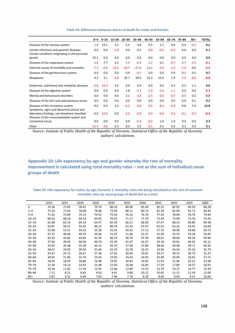
108

Table 34: Differences between shares of death for males and females

0–4 5–14 15–24 25–34 35–44 45–54 55–64 65–74 75–84 85+ TOTAL

Diseases of the nervous system -1.0 23.1 2.2 2.5 4.8 0.5 1.1 0.6 0.4 -0.2 0.2

Certain infectious and parasitic diseases 0.0 0.0 -1.0 0.0 0.2 -0.9 -0.2 -0.2 0.6 0.0 0.1 Certain conditions originating in the perinatal period 32.1 0.0 0.0 0.0 0.0 0.0 0.0 0.0 0.0 0.0 0.0

Diseases of the respiratory system -2.6 7.7 4.2 -1.5 -0.3 -1.2 0.1 -0.7 -2.7 -4.5 -0.1

External causes of morbidity and mortality -7.7 -6.9 -13.2 -24.7 -27.8 -13.2 -4.0 -1.5 -1.2 0.6 -5.4

Diseases of the genitourinary system 0.0 0.0 0.0 0.0 -0.3 0.0 0.0 0.9 0.1 0.5 0.7

Neoplasms 4.2 3.1 -4.8 20.7 28.0 31.3 13.4 1.9 -7.5 -6.0 -6.0

Endocrine, nutritional and metabolic diseases -2.6 -

12.3 3.2 0.0 0.9 0.9 0.5 0.3 0.5 1.1 0.6

Diseases of the digestive system 0.0 0.0 0.0 1.8 -4.3 -5.9 -2.6 -1.1 0.0 0.6 -2.3

Mental and behavioural disorders 0.0 0.0 0.0 2.1 -1.8 -2.4 -0.5 -0.7 -0.5 0.2 -0.8

Diseases of the skin and subcutaneous tissue 0.0 0.0 0.0 0.0 0.0 0.0 0.0 0.5 0.0 0.1 0.2

Diseases of the circulatory system 0.0 0.0 3.2 -6.2 -0.6 -8.5 -8.2 -0.9 9.8 7.6 12.8 Symptoms, signs and abnormal clinical and laboratory findings, not elsewhere classified 0.0

-10.0 0.0 -3.2 -0.9 -0.5 -0.9 -0.3 -0.1 -0.3 -0.4

Diseases of the musculoskeletal system and connective tissue 0.0 0.0 0.0 0.0 -0.3 -0.2 1.0 1.0 0.4 0.0 0.3

Other -22.4 -4.6 6.3 8.5 2.5 -0.1 0.1 0.4 0.1 0.3 0.1



Appendix 10: Life expectancy by age and gender whereby the rate of mortality improvement is calculated using total mortality rates – not as the sum of individual cause groups of death

Table 35: Life expectancy for males, by age; Scenario 1, mortality rates not being calculated as the sum of assumed mortality rates by cause groups of death but as a total

2010 2015 2020 2025 2030 2035 2040 2045 2050 2055 2060

0 76.36 77.85 78.91 79.70 80.33 80.96 81.60 82.25 82.91 83.59 84.28 1–4 75.56 77.03 78.08 78.86 79.49 80.11 80.74 81.39 82.04 82.71 83.40 5–9 71.62 73.09 74.13 74.92 75.54 76.16 76.79 77.43 78.09 78.76 79.44 10–14 66.63 68.10 69.14 69.92 70.55 71.17 71.79 72.44 73.09 73.76 74.45 15–19 61.68 63.14 64.19 64.97 65.59 66.21 66.83 67.47 68.13 68.80 69.48 20–24 56.87 58.31 59.35 60.12 60.74 61.35 61.97 62.61 63.25 63.92 64.60 25–29 52.08 53.51 54.53 55.30 55.91 56.52 57.13 57.76 58.40 59.06 59.73 30–34 47.27 48.68 49.70 50.46 51.07 51.66 52.27 52.90 53.53 54.18 54.85 35–39 42.43 43.82 44.83 45.59 46.19 46.79 47.39 48.01 48.64 49.29 49.96 40–44 37.68 39.03 40.04 40.79 41.39 41.97 42.57 43.18 43.81 44.45 45.11 45–49 33.05 34.38 35.38 36.12 36.70 37.28 37.86 38.46 39.08 39.71 40.36 50–54 28.67 29.95 30.93 31.66 32.23 32.78 33.35 33.94 34.54 35.16 35.79 55–59 24.47 25.72 26.67 27.38 27.92 28.46 29.01 29.57 30.15 30.75 31.37 60–64 20.65 21.83 22.74 23.42 23.93 24.43 24.95 25.49 26.04 26.62 27.21 65–69 16.95 18.03 18.86 19.48 19.95 20.43 20.92 21.43 21.96 22.51 23.08 70–74 13.36 14.23 14.93 15.48 15.93 16.38 16.85 17.34 17.84 18.37 18.92 75–79 10.34 11.02 11.59 12.05 12.46 12.89 13.33 13.79 14.27 14.77 15.29 80–84 7.71 8.21 8.65 9.03 9.41 9.80 10.22 10.65 11.11 11.59 12.09 85+ 5.87 6.31 6.69 7.03 7.40 7.78 8.18 8.60 9.04 9.51 10.00



109

Table 36: Life expectancy for females, by age; Scenario 1, mortality rates not being calculated as the sum of assumed mortality rates by cause groups of death but as a total

2010 2015 2020 2025 2030 2035 2040 2045 2050 2055 2060

0 83.13 84.33 85.21 85.89 86.49 87.10 87.72 88.37 89.03 89.72 90.43 1–4 82.30 83.47 84.35 85.03 85.62 86.22 86.84 87.48 88.14 88.82 89.52 5–9 78.32 79.49 80.36 81.04 81.63 82.23 82.85 83.49 84.15 84.83 85.53 10–14 73.39 74.55 75.42 76.10 76.69 77.29 77.90 78.54 79.19 79.87 80.58 15–19 68.42 69.58 70.44 71.12 71.71 72.31 72.92 73.56 74.21 74.89 75.59 20–24 63.49 64.64 65.50 66.18 66.77 67.36 67.97 68.61 69.26 69.94 70.64 25–29 58.54 59.68 60.54 61.22 61.81 62.40 63.01 63.64 64.29 64.97 65.67 30–34 53.61 54.75 55.60 56.28 56.86 57.45 58.06 58.69 59.34 60.01 60.71 35–39 48.70 49.83 50.68 51.35 51.93 52.52 53.13 53.75 54.40 55.07 55.77 40–44 43.80 44.92 45.77 46.44 47.02 47.60 48.20 48.83 49.47 50.14 50.83 45–49 38.98 40.08 40.92 41.58 42.15 42.73 43.33 43.95 44.59 45.26 45.94 50–54 34.23 35.29 36.12 36.78 37.34 37.92 38.51 39.12 39.76 40.41 41.10 55–59 29.72 30.75 31.56 32.21 32.76 33.32 33.89 34.49 35.12 35.76 36.44 60–64 25.24 26.23 27.02 27.64 28.18 28.72 29.29 29.88 30.49 31.12 31.79 65–69 20.91 21.84 22.58 23.17 23.69 24.22 24.78 25.35 25.95 26.57 27.22 70–74 16.73 17.56 18.24 18.80 19.30 19.81 20.35 20.91 21.49 22.10 22.74 75–79 12.86 13.58 14.18 14.68 15.16 15.66 16.18 16.72 17.29 17.88 18.50 80–84 9.57 10.18 10.70 11.15 11.61 12.08 12.58 13.10 13.65 14.23 14.83 85+ 7.06 7.63 8.11 8.52 8.96 9.43 9.91 10.42 10.96 11.52 12.12



Appendix 11: Results of Scenarios 2 and 3 – Annual rate of improvement in mortality [%], mortality rate of standard population [%] and life expectancy


0.0

0.5

1.0

1.5

2.0

2.5

3.0

2010 2015 2020 2025 2030 2035 2040 2045 2050 2055 2060

Ann

ual r

ate

of im

prov

emen

t in

mor

talit

y [%

]

Year

Males

Circulatory

Neoplasms

External

All other causes

0

1

2

3

4

5

6

7

8

9

2010 2015 2020 2025 2030 2035 2040 2045 2050 2055 2060

Mor

taliy

rat

e of

sta

ndar

d po

pula

tion

[%

],

deco

mpo

sed

by c

ause

of

deat

h

Year

Males

Circulatory

Neoplasms

External

All other causes

0.0

0.5

1.0

1.5

2.0

2.5

2010 2015 2020 2025 2030 2035 2040 2045 2050 2055 2060

Ann

ual r

ate

of im

prov

emen

t in

mor

talit

y [%

]

Year

Females

Circulatory

Neoplasms

External

All other causes

0

1

2

3

4

5

6

7

8

9

2010 2015 2020 2025 2030 2035 2040 2045 2050 2055 2060

Mor

taliy

rat

e of

sta

ndar

d po

pula

tion

[%

],

deco

mpo

sed

by c

ause

of

deat

h

Year

FemalesCirculatory

Neoplasms

External

All other causes


110

Table 37: Life expectancy for males, by age; Scenario 2, mortality rates are calculated as a sum of assumed mortality rates by cause groups of death

2010 2015 2020 2025 2030 2035 2040 2045 2050 2055 2060

0 76.31 77.60 78.42 78.99 79.42 79.83 80.24 80.65 81.07 81.49 81.91 1–4 75.50 76.76 77.58 78.15 78.57 78.98 79.39 79.80 80.21 80.63 81.04 5–9 71.56 72.82 73.64 74.20 74.63 75.03 75.44 75.85 76.26 76.68 77.09 10–14 66.57 67.83 68.64 69.21 69.63 70.04 70.45 70.86 71.27 71.68 72.10 15–19 61.62 62.88 63.69 64.26 64.68 65.08 65.49 65.90 66.31 66.72 67.14 20–24 56.81 58.05 58.86 59.42 59.84 60.25 60.65 61.05 61.46 61.87 62.28 25–29 52.03 53.26 54.07 54.62 55.04 55.44 55.84 56.24 56.64 57.05 57.46 30–34 47.21 48.43 49.23 49.79 50.20 50.59 50.99 51.39 51.79 52.19 52.60 35–39 42.38 43.59 44.39 44.94 45.35 45.74 46.14 46.53 46.93 47.33 47.73 40–44 37.63 38.81 39.61 40.16 40.56 40.95 41.34 41.73 42.13 42.52 42.92 45–49 33.02 34.18 34.97 35.51 35.91 36.29 36.67 37.06 37.45 37.84 38.23 50–54 28.63 29.76 30.54 31.08 31.46 31.83 32.21 32.58 32.96 33.34 33.72 55–59 24.44 25.52 26.29 26.81 27.18 27.54 27.89 28.25 28.62 28.98 29.35 60–64 20.61 21.64 22.37 22.86 23.21 23.54 23.88 24.21 24.55 24.90 25.25 65–69 16.92 17.86 18.52 18.97 19.29 19.60 19.91 20.22 20.54 20.86 21.19 70–74 13.33 14.07 14.61 15.00 15.29 15.58 15.87 16.16 16.46 16.76 17.07 75–79 10.32 10.89 11.32 11.63 11.89 12.14 12.40 12.67 12.94 13.22 13.50 80–84 7.69 8.10 8.41 8.65 8.88 9.11 9.34 9.59 9.83 10.09 10.35 85+ 5.84 6.18 6.43 6.63 6.84 7.05 7.27 7.49 7.72 7.95 8.20



Table 38: Life expectancy for females, by age; Scenario 2, mortality rates are calculated as a sum of assumed mortality rates by cause groups of death

2010 2015 2020 2025 2030 2035 2040 2045 2050 2055 2060

0 83.05 83.99 84.63 85.09 85.48 85.86 86.24 86.63 87.02 87.41 87.81

1–4 82.23 83.17 83.80 84.27 84.65 85.03 85.41 85.79 86.18 86.57 86.96

5–9 78.25 79.19 79.82 80.28 80.66 81.04 81.42 81.80 82.19 82.58 82.97

10–14 73.32 74.26 74.89 75.35 75.73 76.11 76.49 76.87 77.25 77.64 78.03

15–19 68.35 69.29 69.92 70.38 70.76 71.13 71.51 71.89 72.28 72.66 73.05

20–24 63.43 64.36 64.98 65.44 65.82 66.20 66.57 66.95 67.33 67.72 68.11

25–29 58.48 59.40 60.03 60.49 60.86 61.24 61.61 61.99 62.37 62.76 63.14

30–34 53.55 54.47 55.10 55.55 55.93 56.30 56.67 57.05 57.43 57.81 58.20

35–39 48.64 49.56 50.18 50.63 51.01 51.38 51.75 52.12 52.50 52.88 53.27

40–44 43.75 44.65 45.27 45.72 46.09 46.46 46.83 47.20 47.58 47.96 48.34

45–49 38.92 39.81 40.42 40.87 41.24 41.60 41.96 42.33 42.71 43.08 43.46

50–54 34.18 35.03 35.64 36.08 36.44 36.80 37.16 37.52 37.89 38.26 38.63

55–59 29.67 30.50 31.09 31.52 31.87 32.21 32.56 32.91 33.26 33.62 33.98

60–64 25.19 25.99 26.56 26.97 27.31 27.64 27.97 28.31 28.65 29.00 29.35

65–69 20.87 21.61 22.14 22.52 22.84 23.16 23.47 23.80 24.13 24.46 24.80

70–74 16.69 17.35 17.82 18.18 18.47 18.77 19.08 19.38 19.70 20.02 20.34

75–79 12.83 13.40 13.81 14.12 14.40 14.68 14.96 15.25 15.55 15.85 16.16

80–84 9.54 10.02 10.36 10.63 10.88 11.14 11.40 11.67 11.95 12.23 12.52

85+ 7.03 7.44 7.73 7.96 8.20 8.44 8.70 8.95 9.22 9.49 9.77



111




0

1

2

3

4

5

6

7

8

9

2010 2015 2020 2025 2030 2035 2040 2045 2050 2055 2060

Mo

rtal

iy r

ate

of s

tand

ard

popu

lati

on [

%],

de

com

pose

d by

cau

se o

f de

ath

Year

Males

Circulatory

Neoplasms

External

All other causes

0.0

0.5

1.0

1.5

2.0

2.5

2010 2015 2020 2025 2030 2035 2040 2045 2050 2055 2060

An

nu

al r

ate

of i

mp

rove

men

t in

mo

rtal

ity

[%]

Year

Females

Circulatory

Neoplasms

External

All other causes

0.0

0.5

1.0

1.5

2.0

2.5

3.0

2010 2015 2020 2025 2030 2035 2040 2045 2050 2055 2060

An

nu

al r

ate

of i

mp

rove

men

t in

mo

rtal

ity

[%]

Year

Males

Circulatory

Neoplasms

External

All other causes

0

1

2

3

4

5

6

7

8

9

2010 2015 2020 2025 2030 2035 2040 2045 2050 2055 2060

Mo

rtal

iy r

ate

of s

tand

ard

popu

lati

on [

%],

de

com

pose

d by

cau

se o

f de

ath

Year

Females

Circulatory

Neoplasms

External

All other causes

112

Table 39: Life expectancy for males, by age; Scenario 3, mortality rates are calculated as a sum of assumed mortality rates by cause groups of death

2010 2015 2020 2025 2030 2035 2040 2045 2050 2055 2060

0 76.33 77.79 78.95 79.98 80.94 81.90 82.90 83.94 85.01 86.13 87.29 1–4 75.52 76.95 78.10 79.12 80.07 81.03 82.02 83.05 84.11 85.22 86.38 5–9 71.58 73.01 74.15 75.17 76.11 77.07 78.06 79.08 80.15 81.26 82.41 10–14 66.59 68.01 69.16 70.18 71.12 72.08 73.07 74.09 75.15 76.26 77.42 15–19 61.64 63.06 64.21 65.22 66.16 67.11 68.10 69.12 70.18 71.29 72.44 20–24 56.83 58.23 59.37 60.37 61.30 62.25 63.23 64.24 65.30 66.39 67.54 25–29 52.05 53.44 54.56 55.55 56.47 57.41 58.38 59.38 60.43 61.52 62.66 30–34 47.23 48.60 49.71 50.70 51.61 52.54 53.50 54.50 55.54 56.62 57.76 35–39 42.40 43.76 44.86 45.84 46.74 47.66 48.62 49.61 50.64 51.72 52.86 40–44 37.65 38.98 40.07 41.03 41.93 42.84 43.79 44.77 45.79 46.87 47.99 45–49 33.03 34.33 35.41 36.35 37.23 38.13 39.06 40.03 41.04 42.10 43.21 50–54 28.65 29.90 30.95 31.87 32.72 33.60 34.51 35.45 36.44 37.48 38.58 55–59 24.45 25.65 26.66 27.56 28.38 29.22 30.10 31.02 31.98 33.00 34.07 60–64 20.62 21.76 22.72 23.57 24.35 25.15 25.99 26.87 27.80 28.78 29.82 65–69 16.93 17.98 18.86 19.65 20.38 21.14 21.94 22.78 23.68 24.63 25.64 70–74 13.34 14.19 14.95 15.66 16.35 17.07 17.84 18.65 19.52 20.44 21.42 75–79 10.33 11.01 11.64 12.28 12.92 13.60 14.32 15.09 15.92 16.81 17.76 80–84 7.70 8.21 8.74 9.30 9.90 10.54 11.23 11.97 12.76 13.62 14.54 85+ 5.85 6.30 6.79 7.32 7.89 8.51 9.18 9.90 10.68 11.52 12.42



Table 40: Life expectancy for females, by age; Scenario 3, mortality rates are calculated as a sum of assumed mortality rates by cause groups of death

2010 2015 2020 2025 2030 2035 2040 2045 2050 2055 2060

0 83.07 84.17 85.13 86.05 86.97 87.93 88.93 89.99 91.09 92.27 93.51 1–4 82.25 83.35 84.29 85.21 86.12 87.07 88.06 89.10 90.21 91.37 92.61 5–9 78.27 79.36 80.31 81.22 82.13 83.08 84.07 85.12 86.22 87.38 88.61 10–14 73.34 74.43 75.38 76.29 77.19 78.14 79.12 80.17 81.26 82.42 83.66 15–19 68.37 69.46 70.40 71.31 72.22 73.16 74.14 75.18 76.28 77.44 78.67 20–24 63.45 64.53 65.47 66.37 67.27 68.21 69.19 70.23 71.32 72.48 73.71 25–29 58.49 59.57 60.51 61.41 62.31 63.24 64.22 65.26 66.35 67.51 68.73 30–34 53.57 54.64 55.57 56.47 57.36 58.30 59.27 60.31 61.40 62.55 63.77 35–39 48.66 49.72 50.65 51.54 52.43 53.36 54.34 55.36 56.45 57.60 58.82 40–44 43.77 44.81 45.74 46.62 47.51 48.43 49.41 50.43 51.51 52.66 53.88 45–49 38.94 39.97 40.88 41.76 42.64 43.56 44.52 45.54 46.62 47.76 48.97 50–54 34.19 35.19 36.09 36.96 37.82 38.73 39.69 40.70 41.77 42.90 44.11 55–59 29.69 30.66 31.53 32.38 33.23 34.11 35.05 36.04 37.10 38.22 39.41 60–64 25.21 26.14 26.99 27.82 28.64 29.51 30.43 31.41 32.44 33.55 34.73 65–69 20.88 21.76 22.56 23.36 24.16 25.01 25.91 26.86 27.88 28.97 30.13 70–74 16.70 17.49 18.24 19.00 19.78 20.60 21.48 22.41 23.41 24.48 25.63 75–79 12.84 13.54 14.23 14.94 15.69 16.48 17.33 18.25 19.22 20.27 21.39 80–84 9.56 10.16 10.78 11.45 12.16 12.93 13.75 14.63 15.59 16.61 17.71 85+ 7.04 7.59 8.17 8.81 9.50 10.25 11.05 11.92 12.85 13.86 14.95



slovenian annuity tables

Documents