sliding mode control using neural networkscdn.intechweb.org/pdfs/15230.pdf · sliding mode control...
TRANSCRIPT
27
Sliding Mode Control Using Neural Networks
Muhammad Yasser, Marina Arifin and Takashi Yahagi Research Institute of Signal Processing
Japan
1. Introduction
Variable structure control with sliding mode, which is commonly known as sliding mode
control (SMC), is a nonlinear control strategy that is well known for its robust characteristics
(Utkin, 1977). The main feature of SMC is that it can switch the control law very fast to drive
the system states from any initial state onto a user-specified sliding surface, and to maintain
the states on the surface for all subsequent time (Utkin, 1977), (Phuah et al., 2005 a).
The conventional SMC has two disadvantages (Ertugrul & Kaynak, 2000), (Slotine & Sastry,
1983), which are the chattering phenomenon (Slotine & Sastry, 1983), (Young et al., 1999)
and the difficulty in calculating the equivalent control law of SMC that requires a thorough
knowledge of the parameters and dynamics of the nominal controlled plant (Ertugrul &
Kaynak, 2000), (Slotine & Sastry, 1983), (Hussain & Ho, 2004).
Many methods of SMC using neural networks (NN) have been proposed (Phuah et al., 2005
a), (Ertugrul & Kaynak, 2000), (Hussain & Ho, 2004), (Phuah et al., 2005 b), (Yasser et al.,
2007), (Topalov et al., 2007).
In this paper, sliding mode controls using NN are proposed to deal with the problem of
eliminating the chattering effect and the difficulty in calculating the equivalent control law
of SMC that requires a thorough knowledge of the parameters and dynamics of the nominal
controlled plant. The first method of this method applies a method using a simplified form
of the distance function proposed in (Phuah et al., 2005 a), (Phuah et al., 2005 b).
Furthermore, the simplified distance function of our method uses a sliding surface in the
space of the output error and its derivations, as proposed in (Yasser et al., 2006 a), (Yasser et
al., 2006 c), instead of the space of the states error to construct a corrective control input.
Thus, no observer is required in the proposed method. Moreover, we also propose the
application of an NN to construct the equivalent control input of SMC. The weights of the
NN are adjusted using a backpropagation algorithm as in (Yasser et al., 2006 b). Hence, a
thorough knowledge of the parameters and dynamics of the nominal controlled plant is not
required for calculating the equivalent control law. Finally, a stability analysis is carried out,
and the effectiveness of this first control method is confirmed through computer
simulations. This first method has been previously discussed in (Yasser et al., 2007).
The second method of this paper applies an NN to produce the gain of the corrective control of SMC. Furthermore, the output of the switching function the corrective control of SMC is applied for the learning and training of the NN. There is no equivalent control of SMC is used in this second method. As in the first method, this second method applies a method using a sliding surface in the space of the output error and its derivations, as proposed in
www.intechopen.com

Sliding Mode Control
510
(Yasser et al., 2006 a), (Yasser et al., 2006 c). The weights of the NN are adjusted using a sliding mode backpropagation algorithm, that is a backpropagation algorithm using the switching function of SMC for its plant sensitivity. Thus, this second method does not use the equivalent control law of SMC, instead it uses a variable corrective control gain produced by the NN for the SMC. Hence, a thorough knowledge of the parameters and dynamics of the nominal controlled plant is not required for calculating the control law. Finally, a stability analysis is carried out, and the effectiveness of this first control method is confirmed through computer simulations.
2. Sliding mode control
In designing a standard sliding mode controller, first we are required to construct a sliding surface that represents a desired system dynamics, and then to develop a switching control law such that a sliding mode exists on every point of the sliding surface. Any states outside the surface are driven to reach the surface in a finite time. Let us consider an SISO nonlinear plant with BIBO described as
( ) ( ( )) ( )
( ) ( ) ( ( ))
p p p p
p p p p
t t B u t
y t C t h t
= += +
x f x
x x
$ (1)
where ( )p tx is an pn th-order plant state vector, ( )pu t is the control input, ( )py t is a plant
output, ( )⋅f is a nonlinear vector function pnR∈ , ( )h ⋅ is a scalar nonlinear function, and pB
and pC are matrices with appropriate dimensions. We assume that the system in (1) is
controllable and observable.
The control objective is to determine a control law ( )pu t such that the state vector ( )p tx
tracks a given bounded desired state vector ˆ ( ) pnp t R∈x . Therefore, the states error can be
obtained as
( 1)
ˆ( ) ( ) ( )
( ), ( ), , ( )
p
p
p p p
x p p
Tnx x x
t t t
e t e t e t−
= −⎡ ⎤= ⎢ ⎥⎣ ⎦
e x x
$ A. (2)
Then the sliding surface in the space of the state error can be obtained as
( ) ( )p p p
Tx x xS t t= c e (3)
where 1 2, , ,
p p p p p
T
x x x x nc c c⎡ ⎤= ⎣ ⎦c A is a slope of sliding surface. Generally pxc is chosen to
force the state error converge to zero when the state is on the sliding surface.
Meanwhile, the process of SMC can be divided into two phases: the approaching phase with
( ) 0pxS t ≠ and the sliding phase with ( ) 0
pxS t = . Therefore, two types of control law: an
equivalent control and a corrective control can be derived separately corresponding to those
two phases.
In the sliding phase, we have ( ) 0pxS t = and ( ) 0
pxS t =$ , then the equivalent control term
( )equ t will force the system dynamics to stay on sliding surface. The equivalent control
( )equ t can be obtained as
www.intechopen.com
Sliding Mode Control Using Neural Networks
511
1
ˆ( ) ( ) ( ( ))p p p
T T Teq x p x p x pu t B t t
−⎡ ⎤ ⎡ ⎤= −⎣ ⎦ ⎣ ⎦c c x c f x$ . (4)
In the approaching phase, where ( ) 0S t ≠ , a corrective control term ( )cu t will force the state
error outside the surface to reach the surface. The corrective control term ( )cu t is defined as
( )( ) ( )pc s xu t k sign S t= (5)
where sk is a positive gain constant, and ( )( )pxsign S t is a sign function defined as
( ) 1, if ( ) 0
( ) 0, if ( ) 0
1, if ( ) 0
p
p p
p
x
x x
x
S t
sign S t S t
S t
⎧+ >⎪⎪= =⎨⎪− <⎪⎩. (6)
Then, the control law of SMC will be expressed as
( ) ( ) ( )p eq cu t u t u t= + . (7)
3. Sliding mode control using Neural Networks and a simplified distance function
The first method of this method applies a method using a simplified form of the distance function proposed in (Phuah et al., 2005 a), (Phuah et al., 2005 b). An NN is applied to construct the equivalent control input of SMC. The weights of the NN are adjusted using a backpropagation algorithm as in (Yasser et al., 2006 b).
3.1 Chattering elimination using a simplified distance function
Based on the concept of point to hyperplane distance, an alternative control method to calculate the corrective control term ( )cu t has been proposed in (Phuah et al., 2005 a), (Phuah et al., 2005 b) to suppress the chattering phenomenon which is caused by high frequency oscillations exhibited by the corrective control law ( )cu t in (5). This method uses a distance function ( )h t to calculate the distance between the trajectory of the state error and the sliding surface to generate the corrective control law. The distance function ( )h t is defined as (Phuah et al., 2005 a), (Phuah et al., 2005)
1
( ) ( )p px xh t S t−= c (8)
where ⋅ is the usual Euclidean norm in pnR . The corrective control law is defined as
(Phuah et al., 2005 a), (Phuah et al., 2005)
( ) ( )cu t kh t= (9)
where k is a positive constant. To construct the corrective control law, the distance function (8) can be simplified to minimize the calculation process, and modified by applying the sliding surface in the space
www.intechopen.com
Sliding Mode Control
512
of the output error and its derivations, proposed in (Yasser et al., 2006 a), (Yasser et al., 2006 c), instead of the state error. For that, first, we consider a linear reference model to which the plant output required to follow in the form
( ) ( ) ( )
( ) ( )m m m m
m m m
t A t B u t
y t C t
= +=mx x
x
$ (10)
where ( )m tx is an mn th-order reference model state vector, ( )mu t is a reference model
input, ( )my t is a reference model output, mA , mC are matrices with appropriate
dimensions, and mB is a scalar value. The reference model can be independent of the
controlled plant, and it is permissible to assume m pn n2 . Then, we define the output error
( )pye t as
( ) ( ) ( )py m pe t y t y t= − (11)
Thus, the simplified distance function ( )simh t can be described as
( ) ( )psim sim yh t k S t= (12)
where simk is a positive constant, and ( )pyS t is a sliding surface in the space of the output
error and its derivations described as (Yasser et al., 2006 a), (Yasser et al., 2006 c)
( 1)
1 2
( ) ( )
, , , ( ), ( ), , ( )
p p p
s
p p p s p p p
Ty y y
Tn
y y y n y y y
S t t
c c c e t e t e t−=
⎡ ⎤⎡ ⎤= ⎢ ⎥⎣ ⎦ ⎣ ⎦
c e
$A A (13)
where 2sn > . Then, by replacing ( )h t in (9) with ( )simh t from (12), a new corrective control law can be defined as
( ) ( ) ( )p pc sim y yu t kh t k S t= = (14)
where py simk k k= ⋅ is a positive constant.
3.2 Neural Networks for equivalent control
To avoid the requirement of the thorough knowledge of the parameters and dynamics of the nominal plant (1), we use a feedforward NN, which consists of an input layer, a hidden layer, and an output layer as in (Yasser et al., 2006 b), to construct the equivalent control input ( )equ t of the SMC in (7). The equivalent control input ( )equ t is described as
( )( ) ( )
( )
eq NN
ZOH NN
u t u t
f u k
αα
== (15)
where α is a positive constant, ( )NNu t is a continuous-time output of the NN, ( )NNu k is a
discrete-time output of the NN, and ( )ZOHf ⋅ is a zero-order hold function. As in (Yasser et al., 2006 b), we implement a sampler in front of the NN with an appropriate sampling period to obtain the discrete-time input of the NN, and a zero-order hold is
www.intechopen.com
Sliding Mode Control Using Neural Networks
513
implemented to transform the discrete-time output ( )NNu k of the NN back to the continuous-time output ( )NNu t of the NN. The input ( )i k of the NN is given as
( ) ( 1), , ( )p py yi k e k e k n⎡ ⎤= − −⎣ ⎦A (16)
where ( )pye k is the discrete-time form of ( )
pye t in (11). And the dynamics of the NN are
given as (Yasser et al., 2006 b)
( ) ( ) ( )q i iqi
h k i k m k=∑ (17)
1
( ) ( )
( ( )) ( )
NN
q qji
u k o k
S h k m k
==∑ (18)
where ( )ii k is the input to the i -th neuron in the input layer ( 1, , ii n= A ), ( )qh k is the input
to the q -th neuron in the hidden layer ( 1, , qq n= A ), ( )o k is the input to the single neuron in
the output layer, in and qn are the number of neurons in the input layer and the hidden
layer, respectively, ( )iqm k are the weights between the input layer and the hidden layer,
( )qjm k are the weights between the hidden layer and the output layer, and 1( )S ⋅ is a
sigmoid function. The sigmoid function is chosen as
1
2( ) 1
1 exp( )S X
Xμ= −+ − (19)
where 0μ > .
The objective of the NN training is to minimize the error function ( )pyE k described as
21 1( ) ( ) ( ) ( )
2 2
j
p p
n
y y m pj
E k e k y k y k⎡ ⎤= = −⎣ ⎦∑ (20)
where ( )pye k is the discrete-time form of ( )
pye t in (11). The NN training is done by adapting
( )iqm k and ( )qjm k using the method in (Yasser et al., 2006 b) as follows
1
( )( )
( )
( ) ( ) ( ( ))
qjqj
m p plant q
E km k c
m k
c y k y k J S h k
∂Δ = − ⋅ ∂⎡ ⎤= ⋅ − ⋅ ⋅⎣ ⎦
(21)
21
( )( )
( )
( ) ( ) ( ) (1 ( )) ( )2
iqiq
m p plant qj i
E km k c
m k
c y k y k J m k S X i kμ
∂Δ = − ⋅ ∂⎡ ⎤= ⋅ − ⋅ ⋅ ⋅ − ⋅⎣ ⎦
(22)
where c is a learning parameter, and plantJ represents the plant Jacobian estimated using
www.intechopen.com
Sliding Mode Control
514
( )
( )
pplant
NN
y kJ sign
u k
∂⎛ ⎞= ⎜ ⎟⎜ ⎟∂⎝ ⎠ (23)
as in (Yasser et al., 2006 b).
3.3 Stability
For the stability analysis of our method, we start by defining its Lyapunov function and its derivation as follows
( ) ( ) ( )
( ) ( ) ( )
SMCNN NN SMC
SMCNN NN SMC
V t V t V t
V t V t V t
= += +$ $ $ (24)
where ( )NNV t is the Lyapunov function of the NN of our method, and ( )SMCV t is the Lyapunov function of SMC of our method.
For ( )NNV t$ , we assume that it can be approximated as
( )
( ) NNNN
V kV t
T
Δ≅ Δ$ (25)
where ( )NNV kΔ is the derivation of a discrete-time Lyapunov function, and TΔ is a sampling time. According to (Yasser et al., 2006 b), ( )NNV kΔ can be guaranteed to be negative definite if the learning parameter c satisfies the following conditions
2
0q
cn
< < (26)
for the weights between the hidden layer and the output layer, ( )qjm k , and
22
0 max ( ) max ( )k qj k iq
c m k i kn
−⎡ ⎤< < ⋅⎣ ⎦ (27)
for the weights between the input layer and the hidden layer, ( )iqm k . Furthermore, if the conditions in (26) and (27) are satisfied, the negativity of ( )NNV t$ can also be increased by reducing TΔ in (25).
For ( )SMCV t , it is defined as
2 ( )( )
2
( ) ( ) ( ).
p
p p
y
SMC
SMC y y
S tV t
V t S t S t
== $$
(28)
Then we the following assumption. Assumption 1: The sliding surface in (13) can approximate the sliding surface in (3) (Yasser et al., 2006 c)
( ) ( )p py xS t S t≅ . (29)
( )SMCV t$ in (28) can be assured to be negative definite if
www.intechopen.com
Sliding Mode Control Using Neural Networks
515
( ) ( )
( )
p p
p p
y x
y y
S t S t
k S t
≅′= −
$ $. (30)
where pyk′ is a positive constant. Following the stability analysis method in (Phuah et al.,
2005 a), we apply (1)—(3), (7), (14), (15), (29) and (30) to (28) and assume that (15) can
approximate (4). Thus, ( )SMCV t$ can be described as
( ) ( ) ( )
( ) ( )
ˆ( ) ( ) ( )
ˆ( ) ( ) ( ( )) ( )
ˆ( ) ( ) ( ( )) ( ) ( )
( ) ( )
p p
p p p
p p
p p p p
p p p p
p p p
p
SMC y x
Ty x x
Ty x p p
T T Ty x p x p x p p
T T Ty x p x p x p eq c
y y y
y
V t S t S t
S t t
S t t t
S t t t B u t
S t t t B u t u t
S t k S t
k
==
⎡ ⎤= −⎣ ⎦⎡ ⎤= − −⎣ ⎦⎡ ⎤⎡ ⎤= − − +⎣ ⎦⎣ ⎦⎡ ⎤= −⎣ ⎦
= −
c e
c x x
c x c f x c
c x c f x c
$$
$
$ $
$
$
2 ( )pyS t
. (31)
which is negative definite, where p p p
Ty x p yk B k= c . The reaching condition (Phuah et al., 2005
a) can be achieved if
( ) ( ( ))p p py y yk S t sign S tη− ≤ . (32)
where η is a small positive constant.
3.4 Simulation
Let us consider an SISO nonlinear plant described by (Yasser et al., 2006 b)
1 2
2 1 1
1 1
0
2 sin( ) 1
sin( )
p
p
x xu
x x x
y x x
⎡ ⎤ ⎡ ⎤ ⎡ ⎤= +⎢ ⎥ ⎢ ⎥ ⎢ ⎥⎣ ⎦ ⎣ ⎦ ⎣ ⎦= +
$$ (33)
and the parameters [ ]12 1p
Ty =c in (13), 20
pyk = in (14), 0.1α = in (15), 1in = in(17),
5qn = in (18), 2μ = in (19), 0.001c = in (21) and (22), 1plantJ = + in (21), and 0.01TΔ = in
(25) are all fixed. The switching speed for the corrective control of SMC is set to 0.02
seconds. We assume a first-order reference model in (10) with parameters 10mA = − ,
10mB = − , and 1mC = .
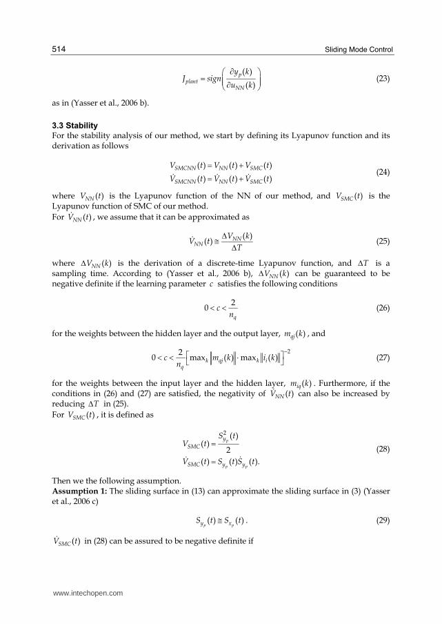
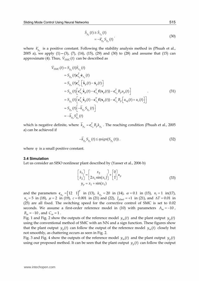
Fig. 1 and Fig. 2 show the outputs of the reference model ( )my t and the plant output ( )py t
using the conventional method of SMC with an NN and a sign function. These figures show
that the plant output ( )py t can follow the output of the reference model ( )my t closely but
not smoothly, as chattering occurs as seen in Fig. 2.
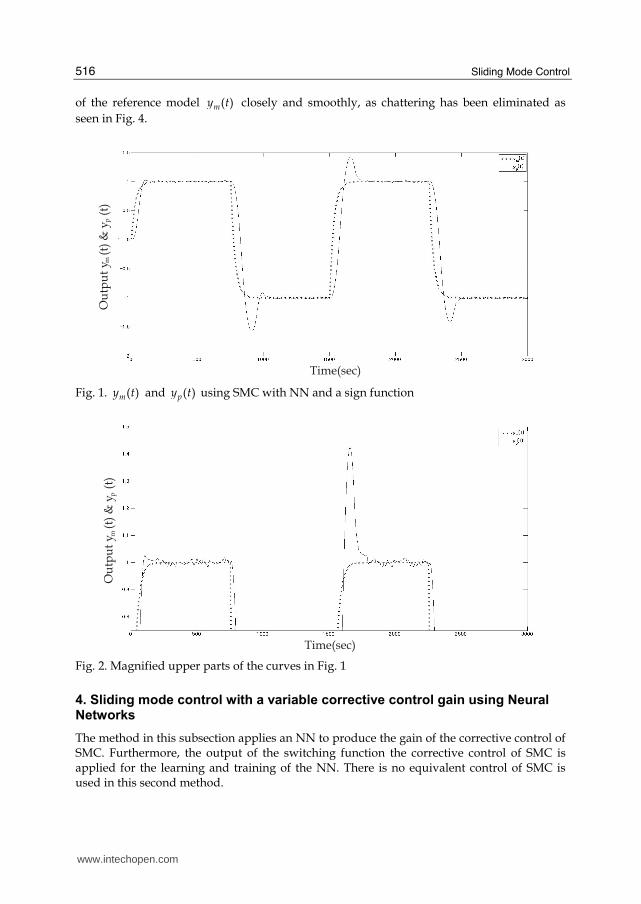
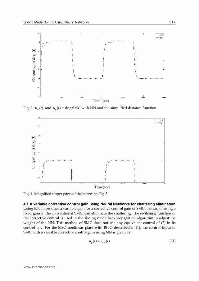
Fig. 3 and Fig. 4 show the outputs of the reference model ( )my t and the plant output ( )py t
using our proposed method. It can be seen that the plant output ( )py t can follow the output
www.intechopen.com
Sliding Mode Control
516
of the reference model ( )my t closely and smoothly, as chattering has been eliminated as
seen in Fig. 4.
Time(sec)
Ou
tpu
t y
(t)
& y
(t)
mp
Fig. 1. ( )my t and ( )py t using SMC with NN and a sign function
Time(sec)
Ou
tpu
t y
(t)
& y
(t)
mp
Fig. 2. Magnified upper parts of the curves in Fig. 1
4. Sliding mode control with a variable corrective control gain using Neural Networks
The method in this subsection applies an NN to produce the gain of the corrective control of SMC. Furthermore, the output of the switching function the corrective control of SMC is applied for the learning and training of the NN. There is no equivalent control of SMC is used in this second method.
www.intechopen.com
Sliding Mode Control Using Neural Networks
517
Ou
tpu
t y
(t)
& y
(t)
mp
Time(sec)
Fig. 3. ( )my t and ( )py t using SMC with NN and the simplified distance function
Ou
tpu
t y
(t)
& y
(t)
mp
Time(sec)
Fig. 4. Magnified upper parts of the curves in Fig. 3
4.1 A variable corrective control gain using Neural Networks for chattering elimination
Using NN to produce a variable gain for a corrective control gain of SMC, instead of using a
fixed gain in the conventional SMC, can eliminate the chattering. The switching function of
the corrective control is used in the sliding mode backpropagation algorithm to adjust the
weight of the NN. This method of SMC does not use any equivalent control of (7) in its
control law. For the SISO nonlinear plant with BIBO described in (1), the control input of
SMC with a variable corrective control gain using NN is given as
( ) ( )p cVu t u t= (34)
www.intechopen.com
Sliding Mode Control
518
( )( ) ( ) ( )p pcV y V yu t k t sign S t= (35)
where ( )cVu t is the corrective control with variable gain using NN, and ( )py Vk t is the
variable gain produced by NN described as
( )( ) ( )
( )
V NNV
ZOH NNV
k t u t
f u k
αα
== (36)
where α is a positive constant, ( )NNVu t is a continuous-time output of the NN, ( )NNVu k is
a discrete-time output of the NN, ⋅ is an absolute function, and ( )ZOHf ⋅ is a zero-order
hold function.
As in subsection 3.2, we implement a sampler in front of the NN with an appropriate
sampling period to obtain the discrete-time input of the NN, and a zero-order hold is
implemented to transform the discrete-time output ( )NNVu k of the NN back to the
continuous-time output ( )NNVu t of the NN. The input ( )i k of the NN is given as in (16), and the dynamics of the NN are given as
( ) ( ) ( )V q i V iqi
h k i k m k=∑ (37)
1
( ) ( )
( ( )) ( )
NNV V
V q Vqji
u k o k
S h k m k
==∑ (38)
where ( )ii k is the input to the i -th neuron in the input layer ( 1, , Vii n= A ), ( )V qh k is the
input to the q -th neuron in the hidden layer ( 1, , Vqq n= A ), ( )Vo k is the input to the single
neuron in the output layer, V in and Vqn are the number of neurons in the input layer and
the hidden layer, respectively, ( )Viqm k are the weights between the input layer and the
hidden layer, ( )Vqjm k are the weights between the hidden layer and the output layer, and
1( )S ⋅ is a sigmoid function. The sigmoid function is chosen as in (19).
4.2 Sliding mode backpropagation for Neural Networks training
In the sliding mode backpropagation, the objective of the NN training is to minimize the
error function ( )pyE k described in (20). The NN training is done by adapting ( )Viqm k and
( )Vqjm k as follows
1
( )( )
( )
( ) ( ) ( ( ))
VqjV qj
m p V plant V q
E km k c
m k
c y k y k J S h k
∂Δ = − ⋅ ∂⎡ ⎤= ⋅ − ⋅ ⋅⎣ ⎦
(39)
21
( )( )
( )
( ) ( ) ( ) (1 ( )) ( )2
ViqViq
m p V plant Vqj i
E km k c
m k
c y k y k J m k S X i kμ
∂Δ = − ⋅ ∂⎡ ⎤= ⋅ − ⋅ ⋅ ⋅ − ⋅⎣ ⎦
(40)
www.intechopen.com
Sliding Mode Control Using Neural Networks
519
where c is the learning parameter, and V plantJ is described as
( )
( )( )
( )( )
( )
p
p
pV plant y
NNV
plant y
y kJ sign sign S k
u k
J sign S k
∂⎛ ⎞= ⋅⎜ ⎟⎜ ⎟∂⎝ ⎠= ⋅
(41)
where ( )pyS k is the time-sampled form of ( )
pyS t in (13).
4.3 Stability
For the stability analysis of our method, we start by defining its Lyapunov function and its derivation as follows
( ) ( ) ( )
( ) ( ) ( )
V V V
V V V
SMCNN NN SMC
SMCNN NN SMC
V t V t V t
V t V t V t
= += +$ $ $ (42)
where ( )NNVV t is the Lyapunov function of the NN of our method, and ( )SMCVV t is the
Lyapunov function of SMC of our method.
For ( )VNNV t$ , we assume that it can be approximated as
( )
( )V
NNVNN
V kV t
T
Δ≅ Δ$ (43)
where ( )NNVV kΔ is the derivation of a discrete-time Lyapunov function, and TΔ is a
sampling time. According to (Yasser et al., 2006 b), ( )NNVV kΔ can be guaranteed to be
negative definite if the learning parameter c satisfies the following conditions
20
Vq
cn
< < (44)
for the weights between the hidden layer and the output layer, ( )Vqjm k , and
22
0 max ( ) max ( )k V qj k iVq
c m k i kn
−⎡ ⎤< < ⋅⎣ ⎦ (45)
for the weights between the input layer and the hidden layer, ( )Viqm k . Furthermore, if the
conditions in (44) and (45) are satisfied, the negativity of ( )VNNV t$ can also be increased by
reducing TΔ in (43).
For ( )SMCVV t , it is defined as
2 ( )( )
2
( ) ( ) ( ).
p
V
V p p
y
SMC
SMC y y
S tV t
V t S t S t
== $$
(46)
Then we again use assumption 1. Thus, ( )VSMCV t$ in (46) can be assured to be negative
definite if
www.intechopen.com
Sliding Mode Control
520
( ) ( )
( )
p p
pV p
y x
y y
S t S t
k S t
≅′= −
$ $. (47)
where pVyk′ is a positive constant. Based on the stability analysis method in subsection 3.3,
we apply (1)—(3), (34), (35), (29) and (30) to (28). Thus, ( )SMCV t$ can be described as
( )
( ) ( ) ( )
( ) ( )
ˆ( ) ( ) ( )
ˆ( ) ( ) ( ( )) ( )
ˆ( ) ( ) ( ( )) ( ) ( )
ˆ( ) (
V p p
p p p
p p
p p p p
p p p p pV p
p p
SMC y x
Ty x x
Ty x p p
T T Ty x p x p x p p
T T Ty x p x p x p y y
Ty x p
V t S t S t
S t t
S t t t
S t t t B u t
S t t t B k t sign S t
S t
==
⎡ ⎤= −⎣ ⎦⎡ ⎤= − −⎣ ⎦⎡ ⎤⎡ ⎤= − − ⎢ ⎥⎢ ⎥⎣ ⎦⎣ ⎦
=
c e
c x x
c x c f x c
c x c f x c
c x
$$
$
$ $
$
$
$ ( )) ( ( )) ( ) ( ) ( )p pV p p
Tx p y y yt t k t S t sign S t⎡ ⎤− −⎣ ⎦c f x
. (48)
where ( ) ( )pV p p
Ty x p y Vk t B k t= c . ( )SMCV t$ in (48) is negative definite if ( )
py Vk t produced by the
NN is large enough. The reaching condition (Phuah et al., 2005 a) can be achieved if
( )ˆ( ) ( ) ( ( )) ( ) ( ) ( ) ( ( ))p p p pV p p p
T Ty x p x p y y y yS t t t k t S t sign S t sign S tη⎡ ⎤− − ≤⎣ ⎦c x c f x$ . (49)
where η is a small positive constant.
4.4 Simulation
Let us consider an SISO nonlinear plant described in (33) and the parameters [ ]9 1p
Ty =c
in (13), 1α = in (36), 2V in = in (37), 5qn = in (38), 2μ = in (19) and (40), 0.01c = in (39)
and (40), 1plantJ = + in (41), and 0.01TΔ = in (43) are all fixed. The switching speed for the
corrective control of SMC is set to 0.02 seconds. We assume a first-order reference model in
(10) with parameters 10mA = − , 10mB = − , and 1mC = .
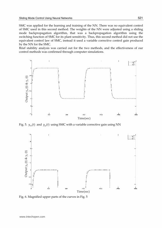
Fig. 5 and Fig. 6 show the outputs of the reference model ( )my t and the plant output ( )py t
using our proposed method. It can be seen that the plant output ( )py t can follow the output
of the reference model ( )my t closely and smoothly, as chattering has been eliminated as
seen in Fig. 6.
5. Conclusion
In this chapter, we proposed two new SMC strategies using NN for SISO nonlinear systems with BIBO has been proposed to deal with the problem of eliminating the chattering effect. In the first method, to eliminate the chattering effect, it applied a method using a simplified distance function. Furthermore, we also proposed the application of an NN using the backpropagation algorithm to construct the equivalent control input of SMC. The second method of this paper applied an NN to produce the gain of the corrective control of SMC. Furthermore, the output of the switching function the corrective control of
www.intechopen.com
Sliding Mode Control Using Neural Networks
521
SMC was applied for the learning and training of the NN. There was no equivalent control of SMC used in this second method. The weights of the NN were adjusted using a sliding mode backpropagation algorithm, that was a backpropagation algorithm using the switching function of SMC for its plant sensitivity. Thus, this second method did not use the equivalent control law of SMC, instead it used a variable corrective control gain produced by the NN for the SMC. Brief stability analysis was carried out for the two methods, and the effectiveness of our control methods was confirmed through computer simulations.
Ou
tpu
t y
(t)
& y
(t)
mp
Time(sec)
Fig. 5. ( )my t and ( )py t using SMC with a variable corrective gain using NN
Ou
tpu
t y
(t)
& y
(t)
mp
Time(sec)
Fig. 6. Magnified upper parts of the curves in Fig. 5
www.intechopen.com
Sliding Mode Control
522
6. References
Ertugrul, M. & Kaynak, O. (2000). Neuro-sliding mode control of robotic manipulators. Mechatronics, Vol. 10, page numbers 239–263, ISSN: 0957-4158
Hussain, M.A. & Ho, P.Y. (2004). Adaptive sliding mode control with neural network based hybrid models. Journal of Process Control, Vol. 14, page numbers 157—176, ISSN: 0959-1524
Phuah, J.; Lu, J. & Yahagi, T. (2005) (a). Chattering free sliding mode control in magnetic levitation system. IEEJ Transactions on Electronics, Information, and Systems, Vol. 125, No. 4, page numbers 600—606, ISSN: 0385-4221
Phuah, J.; Lu, J.; Yasser, M.; & Yahagi, T. (2005) (b). Neuro-sliding mode control for magnetic levitation systems, Proceedings of the 2005 IEEE International Symposium on Circuits and Systems (ISCAS 2005), page numbers 5130—5133, ISBN: 0-7803-8835-6, Kobe, Japan, May 2005, IEEE, USA
Slotine, J.E. & Sastry, S. S. (1983). Tracking control of nonlinear systems using sliding surface with application to robotic manipulators. International Journal of Control, Vol. 38, page numbers 465—492, ISSN: 1366-5820
Topalov, A.V.; Cascella, G.L.; Giordano, V.; Cupertion, F. & Kaynak, O. (2007). Sliding mode neuro-adaptive control of electric drives. IEEE Transactions on Industrial Electronnics, Vol. 54, page numbers 671—679, ISSN: 0278-0046
Utkin, V.I. (1977). Variable structure systems with sliding mode. IEEE Transactions on Automatic Control, Vol. 22, page numbers 212—222 , ISSN: 00189286
Yasser, M.; Trisanto, A.; Lu, J. & Yahagi T.(2006) (a). Adaptive sliding mode control using simple adaptive control for SISO nonlinear systems, Proceedings of the 2006 IEEE International Symposium on Circuits and Systems (ISCAS 2006), page numbers 2153—2156, ISBN: 0-7803-9390-2, Island of Kos, Greece, May 2006, IEEE, USA
Yasser, M.; Trisanto, A.; Haggag, A.; Lu, J.; Sekiya, H. & Yahagi, T. (2006) (c). An adaptive sliding mode control for a class of SISO nonlinear systems with bounded-input bounded-output and bounded nonlinearity, Proceedings of the 45th IEEE Conference on Decision and Control (45th CDC), page numbers 1599–1604, ISBN: 1-4244-0171-2, San Diego, USA, December 2006, IEEE, USA
Yasser, M., Trisanto, A., Lu, J. & Yahagi, T. (2006) (b). A method of simple adaptive control for nonlinear systems using neural networks. IEICE Transactions on Fundamentals, Vol. E89-A, No. 7, page numbers 2009—2018, ISSN: 1745-1337
Yasser, M., Trisanto, A., Haggag, A., Yahagi, T., Sekiya, H. & Lu, J. (2007). Sliding mode control using neural networks for SISO nonlinear systems, Proceedings of The SICE Annual Conference 2007, International Conference on Instrumentation, Control and Information Technology (SICE2007), page numbers 980–984, ISBN: 978-4-907764-27-2, Takamatsu, Japan, September 2007, SICE Japan
Young, K.D.; Utkin, V.I. & Ozguner, U. (1999). A control engineer’s guide to sliding mode control. IEEE Transactions On Control System Technology, Vol. 7, No. 3, ISSN: 1063-6536
www.intechopen.com
Sliding Mode ControlEdited by Prof. Andrzej Bartoszewicz
ISBN 978-953-307-162-6Hard cover, 544 pagesPublisher InTechPublished online 11, April, 2011Published in print edition April, 2011
InTech EuropeUniversity Campus STeP Ri Slavka Krautzeka 83/A 51000 Rijeka, Croatia Phone: +385 (51) 770 447 Fax: +385 (51) 686 166www.intechopen.com
InTech ChinaUnit 405, Office Block, Hotel Equatorial Shanghai No.65, Yan An Road (West), Shanghai, 200040, China
Phone: +86-21-62489820 Fax: +86-21-62489821
The main objective of this monograph is to present a broad range of well worked out, recent applicationstudies as well as theoretical contributions in the field of sliding mode control system analysis and design. Thecontributions presented here include new theoretical developments as well as successful applications ofvariable structure controllers primarily in the field of power electronics, electric drives and motion steeringsystems. They enrich the current state of the art, and motivate and encourage new ideas and solutions in thesliding mode control area.
How to referenceIn order to correctly reference this scholarly work, feel free to copy and paste the following:
Muhammad Yasser, Marina Arifin and Takashi Yahagi (2011). Sliding Mode Control Using Neural Networks,Sliding Mode Control, Prof. Andrzej Bartoszewicz (Ed.), ISBN: 978-953-307-162-6, InTech, Available from:http://www.intechopen.com/books/sliding-mode-control/sliding-mode-control-using-neural-networks