experimental evaluation of sliding-mode control … · experimental evaluation of sliding-mode...

Çukurova Üniversitesi Mühendislik Mimarlık Fakültesi Dergisi, 27(1), ss. 23-37, Haziran 2012 Çukurova University Journal of the Faculty of Engineering and Architecture, 27(1), pp. 23-37, June 2012

Ç.Ü.Müh.Mim.Fak.Dergisi, 27(1), Haziran 2012 23

Experimental Evaluation of Sliding-Mode Control Techniques

Murat FURAT*1

ve İlyas EKER1

1Çukurova University, Electrical and Electronics Eng. Dept., Çukurova University, Adana,

TURKEY

Abstract

Sliding-mode control (SMC) is one of the robust and nonlinear control methods. Systematic design

procedure of the method provides a straightforward solution for the control input. The method has several

advantages such as robustness against matched external disturbances and unpredictable parameter

variations. On the other hand, the chattering is a common problem for the method. Some approaches

have been proposed in the literature to overcome the chattering problem.

In the present paper, an experimental evaluation and practical applicability of conventional (first-order)

sliding-mode control techniques are investigated. Experimental applications are performed using an

electromechanical system for speed tracking control and disturbance regulation problems. The graphical

results are illustrated and the performance measurements are tabulated based on time-domain analysis.

The experimental results indicate the fact that the sliding-mode control is applicable to practical control

systems with the cost of some disadvantages.

Key Words: Conventional sliding-mode control, SMC, chattering, real system application

Kaymalı-Kutup Kontrol Tekniklerinin Deneysel Değerlendirilmesi

Özet

Klasik kayan kipli-kontrol (KKK), doğrusal olmayan ve dayanıklı kontrol yöntemlerinden biridir.

Metodun düzenli tasarım işlemi, kontrol girişi için kolay çözüm sağlar. Bu yöntemin eşleşen dış

bozuculara ve belirsiz parametre değişimlerine karşı dayanıklılığı gibi çeşitli avantajları vardır. Diğer

yandan, çıtırdama bu yöntemin ortak problemidir. Literatürde, çıtırdama problemini aşmak için bazı

yaklaşımlar önerilmiştir.

Bu çalışmada, klasik (birinci derece) KKK yöntemlerin deneysel değerlendirmesi ve pratik

uygulanabilirliği araştırılmıştır. Deneysel uygulamalar, bir elektromekanik sistemin hız kontrolü ve

bozucu ayarlaması üzerine yapılmıştır. Zamana bağlı grafiksel sonuçlar gösterilmiş ve performans

ölçümleri tablolar halinde sunulmuştur. Deneysel sonuçlar, bazı dezavantajlarına rağmen kayan kipli

kontrolün pratik kontrol sistemlerine uygulanabilirliğini göstermiştir.

Anahtar Kelimeler: Klasik kayan-kipli kontrol, KKK, çıtırdama, gerçek sistem uygulaması

* Yazışmaların yapılacağı yazar: Murat FURAT, Çukurova University, Electrical and Electronics Eng.

Dept., Çukurova University, Adana, TURKEY. [email protected]


24 Ç.Ü.Müh.Mim.Fak.Dergisi, 27(1), Haziran 2012

1. Introduction

The control methods, in general, can be classified

into model-based and non-model based methods.

Model-based control methods are systematic and

can be applied to general cases, and specifications

in terms of robustness and tracking accuracy can

be priory assigned, as well as various optimally

criteria can be fulfilled. However, in real systems,

there are many parameters, external disturbances

and uncertainties which are unpredictable and

difficult to model. Therefore, non-model based

control methods are largely applied in practice

since they do not require knowledge of complex

mathematical models. The methods can guarantee

limited performances and robustness of control

system and the design procedure is not systematic

hence in complex systems it can be difficult to

apply. The sliding-mode control method,

theoretically, is able to reject the matched

disturbances and it is able to provide robust control

signal under uncertainties [1].

Sliding-mode control (SMC) is a particular type of

variable structure control which has been studied

extensively for over 50 years [1-4]. The first

publication in the literature may be found in 1977

[1] and sliding-mode control has been one of the

significant interests in the control research

community worldwide [4]. Since it has systematic

design procedure, it is one of the most powerful

solutions for many practical control designs [3]. It

is a robust control scheme based on the concept of

changing the structure of the controller in response

to changing the state of the system in order to

obtain desired output [5]. Therefore SMC is a

successful control method for nonlinear systems.

There are many solution techniques in the

literature for the conventional sliding-mode control

[2,4]. Controller design procedure, number of

control tuning parameters and properties of

subsystems are of interest in these techniques [6].

The method has been applied to several problems

such as automotive, induction motors, automotive

climate control, diesel engine, alternator [3], DC

motors [5], chemical processes [7,12], SMA

actuator [8], submarines [9], electrical drives [10].

Also, numerous SMC techniques were proposed in

the literature to increase the performance of SMC

by combining SMC with soft computing control

methods, i.e. neural networks, fuzzy logic, genetic

algorithm [4].

The contribution of the paper is that the SMC

techniques presented in [1,5,7,12] are

experimented on a real system to demonstrate

applicability of the techniques to practical systems.

The results are presented graphically and

comparison measures based on time-domain

analysis are tabulated.

The present paper is organized as follows. In

Section 2, fundamentals of SMC are outlined. The

experimental setup and experimented SMC

techniques are introduced in Section 3. The

applications of selected SMC techniques to the real

system and graphical results with discussion are

given in Section 4. In the last section, the results of

the experiments are concluded.

2. Fundamentals of Sliding-Mode

Control

Robustness and systematic design procedure are

well-known advantages of sliding-mode

controllers [1,3]. Traditionally, the conventional

sliding-mode control method has been designed

for the systems with relative degree of one. Since

the control input appears in the first derivative of

sliding function, its relative degree with respect to

control is one. This type of sliding-mode control

method is called as first-order SMC.

A first-order sliding-mode controller consists of

two distinct control laws: switching control and

equivalent control [1,3,5]. The most important task

is to design the switching control law which

enforces the system to the sliding surface, ( )s t ,

defined by the user, and to maintain the system

state trajectory on this surface as shown in Fig. 1

in which e and e denote the tracking error and

first-time derivative of the tracking error,

respectively. ‘t’ in ( )s t is the independent variable

time. The dynamic performance of the system is

directly dependent choosing an appropriate

Murat Furat ve İlyas Eker


switching control law. Lyapunov technique is

generally used to determine the stability of the

closed-loop systems [1].

Figure 1. Graphical representation of sliding-mode

control

Ideal sliding-mode can be found by equivalent

control approach [1]. First time derivative of ( )s t

along the system trajectory is set equal to zero and

the resulting algebraic system is solved for the

control law. If the equivalent control exists, it is

substituted into ( )s t and the resulting equations

are the ideal sliding-mode [1].

The first step in the sliding-mode control solution

is to determine a sliding manifold which is also

called sliding surface or sliding function, ( )s t

being a function of the tracking error, ( )e t ,

( )e t R that is the difference between set point

and output measurement, as:

1

( ) ( )

nd

s t e tdt

(1)

where n denotes the order of uncontrolled

system, is a positive constant, R

where R

and R denotes set of real and positive real

numbers, respectively. is the tuning parameter

which determines the slope of sliding manifold.

When the system is in the sliding-mode, both ( )s t

and ( )s t are equal to zero, ( ) ( ) 0s t s t .

The objective is to determine a control law ( )u t ,

so that the tracking error and its derivative should

converge to zero from any initial state to the

equilibrium point in a finite time. ( )u t consists of

two additive signals switching (discontinuous)

signal, ( )sw

u t , and equivalent (continuous) signal,

( )eq

u t , determined separately [1,5]:

( ) ( ) ( )eq sw

u t u t u t (2)

If the initial trajectory is not on the sliding surface,

the switching control, ( )sw

u t , enforces the error

toward the origin of the sliding surface and this is

called the reaching phase. The equivalent control

may not be able to move the system state toward

sliding surface. Therefore, the switching control is

designed on the basis of relay-like function

because it allows changes between the structures

infinitely fast. The equivalent control is found by

equating derivative of sliding function to zero. On

the other hand, the switching control can be

selected directly as [1]:

( ) ( ( ))sw

u t ksign s t (3)

where k is a positive constant that should be large

enough to suppress all matching uncertainties and

unpredictable system dynamics and ( )sign is a

signum function [3].

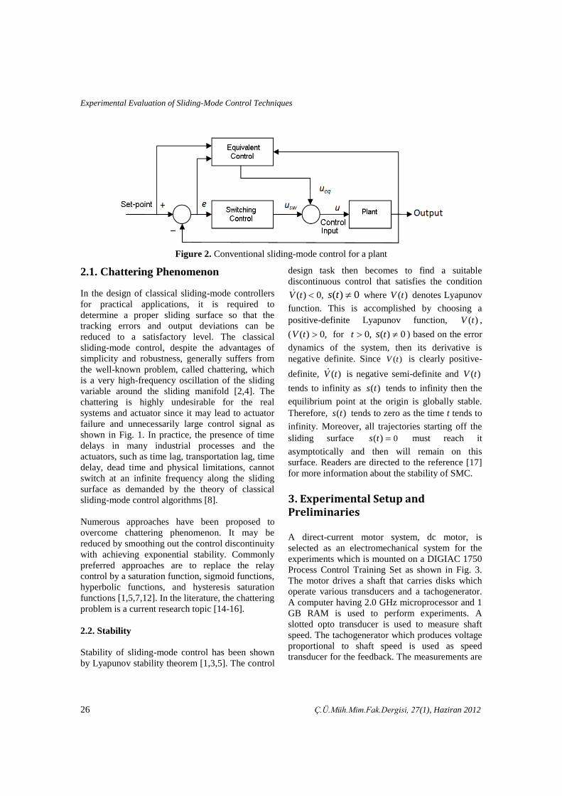
The block diagram of conventional sliding-mode

control method is illustrated in Fig. 2.



Figure 2. Conventional sliding-mode control for a plant

2.1. Chattering Phenomenon

In the design of classical sliding-mode controllers

for practical applications, it is required to

determine a proper sliding surface so that the

tracking errors and output deviations can be

reduced to a satisfactory level. The classical

sliding-mode control, despite the advantages of

simplicity and robustness, generally suffers from

the well-known problem, called chattering, which

is a very high-frequency oscillation of the sliding

variable around the sliding manifold [2,4]. The

chattering is highly undesirable for the real

systems and actuator since it may lead to actuator

failure and unnecessarily large control signal as

shown in Fig. 1. In practice, the presence of time

delays in many industrial processes and the

actuators, such as time lag, transportation lag, time

delay, dead time and physical limitations, cannot

switch at an infinite frequency along the sliding

surface as demanded by the theory of classical

sliding-mode control algorithms [8].

Numerous approaches have been proposed to

overcome chattering phenomenon. It may be

reduced by smoothing out the control discontinuity

with achieving exponential stability. Commonly

preferred approaches are to replace the relay

control by a saturation function, sigmoid functions,

hyperbolic functions, and hysteresis saturation

functions [1,5,7,12]. In the literature, the chattering

problem is a current research topic [14-16].

2.2. Stability

Stability of sliding-mode control has been shown

by Lyapunov stability theorem [1,3,5]. The control

design task then becomes to find a suitable

discontinuous control that satisfies the condition

( ) 0, ( ) 0V t s t where ( )V t denotes Lyapunov

function. This is accomplished by choosing a

positive-definite Lyapunov function, ( )V t ,

( ( ) 0, V t for 0, ( ) 0t ts ) based on the error

dynamics of the system, then its derivative is

negative definite. Since ( )V t is clearly positive-

definite, ( )V t is negative semi-definite and ( )V t

tends to infinity as ( )s t tends to infinity then the

equilibrium point at the origin is globally stable.

Therefore, ( )s t tends to zero as the time t tends to

infinity. Moreover, all trajectories starting off the

sliding surface 0( )s t must reach it

asymptotically and then will remain on this

surface. Readers are directed to the reference [17]

for more information about the stability of SMC.

3. Experimental Setup and Preliminaries

A direct-current motor system, dc motor, is

selected as an electromechanical system for the

experiments which is mounted on a DIGIAC 1750

Process Control Training Set as shown in Fig. 3.

The motor drives a shaft that carries disks which

operate various transducers and a tachogenerator.

A computer having 2.0 GHz microprocessor and 1

GB RAM is used to perform experiments. A

slotted opto transducer is used to measure shaft

speed. The tachogenerator which produces voltage

proportional to shaft speed is used as speed

transducer for the feedback. The measurements are



transmitted from experimental set to the computer

via a data acquisition card (DAQ).

Matlab/Simulink is used for all calculations and

controller design.

DC Motor

Various Speed Transducers

Position Sensor

Tachogenerator

Figure 3. A view of the electromechanical system

The mathematical description of the

electromechanical system is given in appendix

[19]. Since the parameters of the mathematical

model cannot be obtained properly, first-order plus

dead-time model is used to approximate the model

of the electromechanical system. For this purpose,

a step input, ( )u t , of 5.12 Volts in magnitude, in

open-loop conditions, is applied to the armature of

the system and output shaft speed is measured in

rpm. The output steady-state voltage produced by

the tachogenerator is measured to be 4.43 Volts

that corresponds to 1200 rpm output shaft speed. A

second-order system model can be used to

approximate the model of the present system as

[11]:

( )1 ( 1)( 1)

d

p p d

t sKe K

G ss s t s

(4)

where K is the gain, td is the time delay and τp is

the time constant.

Using the input-output plots of the system, the

plant coefficients are found to be

0.0035,d

t 0.145,p

0.86K . The modeling

error is illustrated in Fig. 4 in which +30 rpm and -

18 rpm of speed deviations corresponding to 2.5%

of the modeling error (modeling error= measured

output – model output) including transient and

steady-state outputs.

Figure 4. Modeling error

The experimental results are presented to

demonstrate the performance of selected SMC

techniques which mainly characterize the classical

SMC. The parameters of the controller are tuned

during the experiments, avoiding complicated

calculations which may cause large chattering that



is dangerous for the actuator. As a design

requirement, overshoot at the output is not desired.

Technique I:

The first technique was proposed by Vadim I.

Utkin [1] in 1977. The related sliding surface is

given in Eq. (1). The control signal is sum of the

equivalent signal and switching signal. The

switching signal is selected to be a signum

function with a constant gain of magnitude 1.5

(k=1.5) and the tuning parameter is chosen to

be 13.75.

Technique II:

The second SMC technique is based on PID

sliding surface as [5]:

1 2 30

( ) ( ) ( ) ( )s t k e t k e d k e t

(5)

where the gain parameters are adjusted to be

130,k

21,k

31.1.k The switching control is

selected to be a saturation function whose gain is

3.5 (k=3.5) and 20, where is the thickness

of boundary layer.

( )sw

ksats t

u

(6)

The saturation function in Eq. (6) is defined as [5]:

( ) ( )if 1

( )

( ) ( )if 1

s t s t

s tsat

s t s tsign

(7)

Technique III:

The third technique is proposed for stable

processes [7]. The structural limitations of PI and

PID controllers may not give satisfactory

responses with large time constant or poorly

located complex poles. Because of this reason, a PI

– PD based sliding surface is selected as:

( )( ) ( ) ( ) ( ) ts t ae t b e t dt t ycy d (8)

where the parameters are adjusted to be a=19.5,

b=100, c=9.76, d=0.1. Tangent hyperbolic function

is selected as switching control whose gain is 3.5

(k=3.5) and 20.

Technique IV:

The last technique is presented to regulate the

nonlinear chemical processes [12]. The sliding

surface is given by

( ) ( )

nd

dts t e t dt

(9)

where the tuning parameter is adjusted to be 60.

The proposed switching control is as [12]:

( )

( )dsw K

s tu

s t

(10)

where is chosen to be 3 and the switching

gain,d

K , is 5.2.

4. Experimental Study and Discussion

Controllers of the techniques are implemented

in Matlab/Simulink environment and sample time

is selected to be 5 ms. The set point is adjusted to

be 4.43 Volts corresponding to 1200 rpm shaft

speed. The step responses are illustrated in Fig. 5.



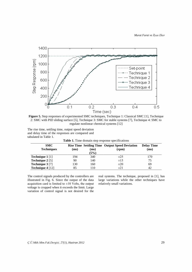
Figure 5. Step responses of experimented SMC techniques, Technique 1: Classical SMC [1], Technique

2: SMC with PID sliding surface [5], Technique 3: SMC for stable systems [7], Technique 4: SMC to

regulate nonlinear chemical systems [12]

The rise time, settling time, output speed deviation

and delay time of the responses are compared and

tabulated in Table 1.

Table 1. Time domain step response specifications

SMC

Techniques

Rise Time

(ms)

Settling Time

(ms)

(5%)

Output Speed Deviation

(rpm)

Delay Time

(ms)

Technique 1 [1] 194 340 ±25 170

Technique 2 [5] 90 140 ±15 75

Technique 3 [7] 130 160 ±20 69

Technique 4 [12] 85 110 ±21 42

The control signals produced by the controllers are

illustrated in Fig. 6. Since the output of the data

acquisition card is limited to ±10 Volts, the output

voltage is cropped when it exceeds the limit. Large

variation of control signal is not desired for the

real systems. The technique, proposed in [1], has

large variations while the other techniques have

relatively small variations.



Figure 6. Control signals of experimented SMC techniques, Technique 1: Classical SMC [1], Technique

2: SMC with PID sliding surface [5], Technique 3: SMC for stable systems [7], Technique 4: SMC to

regulate nonlinear chemical systems [12]

The objective of sliding-mode control is to force

both error and derivative of error to the

equilibrium point. Then the selected sliding

surface, ( )s t , tends to zero in a finite time and the

system states should remain on the surface. In Fig.

7, Fig. 8 and Fig. 9, the selected sliding surfaces

are illustrated. The variations in ( )s t of [1] in Fig. 7

are larger than that of the other techniques. The

sliding surfaces of the techniques in [5,7] converge

faster than others. The slowest one is in [12] as

illustrated in Fig. 9.

Figure 7. Sliding surfaces of experimented SMC techniques, Technique 1: Classical SMC [1]



Figure 8. Sliding surfaces of experimented SMC techniques, Technique 2: SMC with PID sliding surface

[5], Technique 3: SMC for stable systems [7]

Figure 9. Sliding surfaces of experimented SMC techniques,

Technique 4: SMC to regulate nonlinear chemical systems [12]

The error versus derivative of error for each

technique is illustrated in Fig. 10 and Fig. 11.

Since the range (numerical magnitudes) of

derivative of the error in technique 1 [1] is larger

than the other techniques, it is illustrated in

different figure, Fig. 10. The others are illustrated

in Fig. 11.



Figure 10. Error versus derivative of error change of experimented SMC techniques, Technique 1:

Classical SMC [1]

Figure 11. Error versus derivative of error change of experimented SMC techniques, Technique 2: SMC

with PID sliding surface [5], Technique 3: SMC for stable systems [7], Technique 4: SMC to regulate

nonlinear chemical systems [12]



The switching signals of all experimented

techniques are illustrated in Fig. 12. Technique 1

proposed in [1] produced strong switching signal

compared with the others. Since the switching

function is selected as signum function with its

gain 1.5, the switching signal produces ±1.5 Volts

due to disturbances and uncertainties of the real

system. In technique 2 proposed in [5], the

switching signal has smaller variations with

smoothness. The tangent hyperbolic function used

in technique 3 in [7] produces a reasonable signal

compared with the signal produced by the

technique 2. In contrast, the switching signal of

technique 4 in [12] has a constant magnitude but

smallest variation. As a result, using smoothed

switching signals such as saturation function in

technique 2 [5], tangent hyperbolic in technique 3

[7] and a smooth function in technique 4 [12],

defined by the Eq. (10), produces less chattering

whereas it may increase the time required to reach

equilibrium point.

Figure 12. Switching signal of experimented SMC techniques, Technique 1: Classical SMC [1],

Technique 2: SMC with PID sliding surface [5], Technique 3: SMC for stable systems [7], Technique 4:

SMC to regulate nonlinear chemical systems [12]

Performance of the experimented techniques can

be also measured with the index of total variation

of the control signal [18]:

1

( 1) ( )TV

i

u i u i

(11)

where u is the control variable and subscript i

refers to sampled values.

The variation at the controller output, both in

transient-state and steady-state, affects the energy

consumption of the actuator. Also, the magnitude

of the total variance shows the smoothness of the

control signal. Therefore, the controllers should be

designed to generate control actions with TV as

small as possible [18]. In other words,

minimization of TV can be performed by means

of reducing the chattering in the control signal. In

an ideal controller, the control signal at different

times in the steady-state is equal for the same set-

point [18].

Further analysis on the performance of the

techniques can be performed by measuring the



standard deviation of the tracking error, , as

follows:

1

1( ( ) )

N

i

e iN

(12)

where N is the sample number, e denotes the

tracking error and is the mean value of tracking

error.

The standard deviation is a useful property to

understand the variation of the tracking error. In

Table 2, the total variance and standard deviation

measurements are given. The smallest total

variance in magnitude was measured in the

technique [12] since the proposed controller

produced saturated control signal in the transient-

state due to the output limitation of the DAQ (±10

Volts). In fact, the output of the controller in [12]

produces high control signal resulting high TV .

The minimum deviation of the tracking error was

also measured in the technique [12] that results in

most accurate control signal was produced by the

controller.

Table 2. Performance specifications

SMC Techniques Total Variance of Control

Signal

Standard Deviation of Tracking

Error

Technique 1 [1] 647.39 0.8434

Technique 2 [5] 1086.20 0.6390

Technique 3 [7] 40.37 0.6581

Technique 4 [12] 16.43 0.5403

The performance of the techniques were also

compared with the performance indices, such as

[20,21]:

IAE (Integral Absolute Error) : ( )e t dt

ISCI (Integral Squared Control Input) : 2( )u t dt

ISE (Integral Squared Error) : 2( )e t dt

Table 3. Results of performance indices

SMC Techniques IAE ISCI ISE

Technique 1 [1] 0.7892 85.225 2.2854

Technique 2 [5] 0.4876 100.426 1.2578

Technique 3 [7] 0.4591 87.259 1.3622

Technique 4 [12] 0.5241 85.834 1.2382

The maximum integral absolute error and integral

squared error were measured in [1] which means

that that the magnitude of error deviation was

maximum. On the other hand, the integral squared

of control input was measured nearly the same as

in [1,7,12].

5. Conclusions

In this study, selected first-order sliding-mode

control techniques have been applied to an

electromechanical system experimentally to

investigate the applicability of the proposed

techniques. A second-order model is approximated

to use in the experiments since most of real

systems can be represented by a second-order



model. Step response, control signal and switching

signal variations, error versus derivative of error

graphs were obtained to compare the performances

of the techniques. During the experiments, the

parameters were tuned manually since the presence

of chattering may cause a harmful effect on the

system components.

Based on the experimental results and time-domain

analysis tabulated in Table 1 and Table 2, it is

clear that the techniques presented in [5,7,12] have

produced better results than the technique

presented in [1]. The maximum magnitude of

chattering is observed in the Utkin’s technique [1]

that may be harmful for fast actuators if the

switching gain is not adjusted properly. However,

the other techniques have less chattering in the

control signal which can be acceptable for the real

systems. Since the tracking error converges

exponentially to zero under uncertainties, the SMC

techniques presented in [5,7,12] can be candidate

to use in industrial applications as alternative to

commonly used PID controller. In addition, the

first-order sliding-mode control algorithm has

systematic solution. Therefore, it is easy to

understand and apply to real systems. Several

works on SMC techniques were summarized in

[2,4,22]

6. Acknowledgements

The authors would like to acknowledge Institute of

Basic and Applied Sciences and Academic

Research Projects Unit of Çukurova University for

their support to the present work.

7. References

1. Utkin, V. I., “Variable Structure Systems with

Sliding Modes”, IEEE Transaction on

Automatic Control, vol. AC-22, pp. 212-222,

1977.

2. Young, K. D., Utkin, V. I., Özgüner, Ü., “A

Control Engineer’s Guide to Sliding Mode

Control”, IEEE Transaction on Control

Systems Technology, vol. 7, pp. 328-342,

1999.

3. Utkin, V. I., Chang, H. C., “Sliding Mode

Control on Electromechanical Systems”,

Mathematical Problems in Engineering, vol.

8, pp. 451-473, 2002.

4. Xinghou, Y., Kaynak, O., “Sliding-Mode

Control with Soft Computing: A Survey”,

IEEE Transaction on Industrial Electronics

vol. 56, pp. 3275-3285, 2009.

5. Eker, İ., “Sliding Mode Control with PID

Sliding Surface and Experimental Application

to an Electromechanical Plant”, ISA

Transactions, vol. 45, pp. 109-118, 2006.

6. Cavallo, A., Natale, C., “High-Order Sliding

Control of Mechanical Systems: Theory and

Experiments”, Control Engineering Practice,

vol. 2, pp. 1139-1149, 2004.

7. Kaya, İ., “Sliding Mode Control of Stable

Processes”, Industrial & Engineering

Chemistry Research, vol 46, pp. 571-578,

2007.

8. Tai, N. T., Ahn, K. K., “A RBF Neural

network Sliding Mode Control for SMA

Actuator”, International Journal of Control,

Automation, and Systems, vol. 8, pp. 1296-

1305, 2010.

9. Walcko, K. J., Novick, D., Nechyba, M. C.,

“Development of a Sliding Mode Control with

Extended Kalman Filter Estimation for

Subjugator”, Conference on Recent Advances

in Robotics, Florida, USA, 2003.

10. Akpolat, Z. H., Gökbulut, M., “Discrete Time

Adaptive Reaching Law Speed Control of

Electrical Drives”, Electrical Engineering,

vol. 85, pp. 53-58, 2003.

11. Furat, M., Eker, İ., “Computer – Aided

Experimental Modeling of a Real System

Using Graphical Analysis of a Step Response

Data”, Computer Applications in Engineering

Education, DOI: 10.1002/cae.20482

12. Camacho, O., Smith, C. A., “Sliding Mode

Control: An Approach to Regulate Nonlinear

Chemical Processes”, ISA Transactions, vol.

39, pp. 205-218, 2000.

13. Guo, L., Hung, J. Y., Nelms, R. M.,

“Comparative Evaluation of Sliding Mode

Fuzzy Controller and PID Controller for a

Boost Converter”, Electric Power Systems

Research, vol. 81, pp. 99-106, 2011.

http://www.refdoc.fr/?traduire=en&FormRechercher=submit&FormRechercher_Txt_Recherche_name_attr=listeTitreSerie:%20%28Industrial%20&%20engineering%20chemistry%20research%29

http://www.refdoc.fr/?traduire=en&FormRechercher=submit&FormRechercher_Txt_Recherche_name_attr=listeTitreSerie:%20%28Industrial%20&%20engineering%20chemistry%20research%29



14. Husain, A. R., Ahmad, M. N., Yatim, A. M.,

“Chattering-free Sliding Mode Control for an

Active Magnetic Bearing System”, World

Academy of Science, vol. 39, pp. 385-391,

2008.

15. Levant, A., “Chattering Analysis”, IEEE

Transaction on Automatic Control, vol. 55,

no. 6, pp. 1380-1389, 2010.

16. Lee, H., Utkin, V. I., “Chattering Suppression

Methods in Sliding Mode Control Systems”,

Annual Reviews in Control, vol. 31, pp. 179-

188, 2007.

17. Utkin, V. I., Sliding Modes in Control and

Optimization, Springer-Verlag, Moscow,

1991.

18. Klan, P., Gorez, R., PI Controller Design for

Actuator Preservation, Proceedings of the 17th

IFAC World Congress, 2008, Korea, South.

19. Eker, İ., Second-order Sliding Mode Control

with Experimental Application, ISA

Transactions, vol. 49, pp. 394-405, 2010.

20. Seborg D E, Edgar T F, and Mellichamp D A.

Process Dynamics and Control, Wiley, New

York, 1989.

21. Hsiao M Y, Li T H S, Lee J Z, Chao C H, and

Tsai S H. Design of interval type-2 fuzzy

sliding-mode controller, Information Sciences,

2008;178:1696-1716.

22. Yu, X., Wang, B., Li, X., Computer-

Controlled Variable Structure Systems: The

State of Art, IEEE Transaction on Industrial

Informatics, Available online.

8. APPENDIX

Mathematical Model of the Electromechanical

System

The electromechanical system consists of a DC

motor and a tachogenerator connected via a shaft.

There are various speed transducers and a position

sensor on the shaft which can be designated as the

load on the shaft. The electrical and mechanical

equations of the system are as follows [19]:

( ) ( ) ( ) ( )a a a a a m m

dv t L i t R i t K t

dt (13)

( ) ( ) ( ) ( ) ( )m m m s m m f m

dJ t T t T t R t T

dt

(14)

( ) ( ) ( ) ( ) ( )L L s L L d f L

dJ t T t R t T t T

dt

(15)

( ) ( ( ) ( )) ( ( ) ( ))s s m L s m L

T t k t t B t t (16)

( ) ( ), ( ) ( )m m L L

d dt t t t

dt dt (17)

where

av : armature voltage of the motor,

aR : armature resistance,

aL : armature inductance,

ai : armature current,

, m L : rotational speeds of the motor,

, m LJ J : moments of inertia,

, m LR R : coefficients of the viscous friction.

mK : torque coefficient,

mT : generated motor torque,

dT : external load disturbance,

fT : nonlinear friction,

sT : transmitted shaft torque,



Model of the nonlinear friction fT can be obtained by an asymmetrical characteristic as:

2 5

0 1 3 4( ) sgn1( ) sgn 2( )

fT e e

(18)

where 1 5 are positive constants and

0 3 , 1 4 , 2 5 and the functions

sgn1 and sgn2 are defined as:

1 if 0sgn1( )

0 if 0

0 if 0sgn 2( )

-1 if 0

(19)

Block diagram of the electromechanical system is

illustrated in Fig.13.

Figure 13. Block diagram of the electromechanical system

experimental evaluation of sliding-mode control … · experimental evaluation of sliding-mode...

Documents