simulation of hawaiian electric companies feeder … · smart inverter technical working group for...
TRANSCRIPT

NREL is a national laboratory of the U.S. Department of Energy Office of Energy Efficiency & Renewable Energy Operated by the Alliance for Sustainable Energy, LLC This report is available at no cost from the National Renewable Energy Laboratory (NREL) at www.nrel.gov/publications.
Contract No. DE-AC36-08GO28308
Simulation of Hawaiian Electric Companies Feeder Operations with Advanced Inverters and Analysis of Annual Photovoltaic Energy Curtailment Julieta Giraldez, Adarsh Nagarajan, Peter Gotseff, Venkat Krishnan, and Andy Hoke National Renewable Energy Laboratory
Reid Ueda, Jon Shindo, Marc Asano, and Earle Ifuku Hawaiian Electric Company
Technical Report NREL/TP-5D00-68681 Revised September 2017

NREL is a national laboratory of the U.S. Department of Energy Office of Energy Efficiency & Renewable Energy Operated by the Alliance for Sustainable Energy, LLC This report is available at no cost from the National Renewable Energy Laboratory (NREL) at www.nrel.gov/publications.
Contract No. DE-AC36-08GO28308
National Renewable Energy Laboratory 15013 Denver West Parkway Golden, CO 80401 303-275-3000 • www.nrel.gov
Simulation of Hawaiian Electric Companies Feeder Operations with Advanced Inverters and Analysis of Annual Photovoltaic Energy Curtailment Julieta Giraldez, Adarsh Nagarajan, Pete Gotseff, Venkat Krishnan, and Andy Hoke National Renewable Energy Laboratory
Reid Ueda, Jon Shindo, Marc Asano, and Earle Ifuku Hawaiian Electric Company
Prepared under Task No. WRHV.1000
Technical Report NREL/TP-5D00-68681 Revised September 2017

NOTICE
This report was prepared as an account of work sponsored by an agency of the United States government. Neither the United States government nor any agency thereof, nor any of their employees, makes any warranty, express or implied, or assumes any legal liability or responsibility for the accuracy, completeness, or usefulness of any information, apparatus, product, or process disclosed, or represents that its use would not infringe privately owned rights. Reference herein to any specific commercial product, process, or service by trade name, trademark, manufacturer, or otherwise does not necessarily constitute or imply its endorsement, recommendation, or favoring by the United States government or any agency thereof. The views and opinions of authors expressed herein do not necessarily state or reflect those of the United States government or any agency thereof.
This report is available at no cost from the National Renewable Energy Laboratory (NREL) at www.nrel.gov/publications.
Available electronically at SciTech Connect http:/www.osti.gov/scitech
Available for a processing fee to U.S. Department of Energy and its contractors, in paper, from:
U.S. Department of Energy Office of Scientific and Technical Information P.O. Box 62 Oak Ridge, TN 37831-0062 OSTI http://www.osti.gov Phone: 865.576.8401 Fax: 865.576.5728 Email: [email protected]
Available for sale to the public, in paper, from:
U.S. Department of Commerce National Technical Information Service 5301 Shawnee Road Alexandria, VA 22312 NTIS http://www.ntis.gov Phone: 800.553.6847 or 703.605.6000 Fax: 703.605.6900 Email: [email protected]
Cover Photos by Dennis Schroeder: (left to right) NREL 26173, NREL 18302, NREL 19758, NREL 29642, NREL 19795.
NREL prints on paper that contains recycled content.
iii This report is available at no cost from the National Renewable Energy Laboratory at www.nrel.gov/publications.
Errata This report, originally published in July 2017, was revised in September 2017 to correct the following specific results:
• Weekly and annual energy curtailment values from activating grid support functions in rooftop solar PV customers,
• Annual reactive power absorption at the feeder level from volt-VAR/volt-watt,
• Annual energy curtailment from volt-watt when combined with volt-VAR, and
• Annual energy curtailment per solar PV rooftop customer Important caveats to the study were also added in the Executive Summary and Section 5 Summary of Conclusions and Recommendations sections. The updated values and caveats do not change the overall conclusions and recommendations between the two versions of the report.

iv This report is available at no cost from the National Renewable Energy Laboratory at www.nrel.gov/publications.
Acknowledgments The National Renewable Energy Laboratory graciously thanks the Hawaiian Electric Companies for funding this work, providing technical expertise, and choosing NREL for collaboration on this important topic.
Additionally, the authors would like to express appreciation to the members of the Hawai‘i Smart Inverter Technical Working Group for their valuable technical input and collaboration.
Finally, the authors thank Kenny Gruchalla from NREL for his data visualization support, and Carlo Brancucci Martinez-Anido and Barry Mather from NREL for their technical review of this report.

v This report is available at no cost from the National Renewable Energy Laboratory at www.nrel.gov/publications.
Nomenclature or List of Acronyms AI advanced inverter AMI advanced metering infrastructure APS Arizona Public Service CGS customer grid supply COM common object model CPF constant power factor CSI California Solar Initiative CSS customer self supply DER distributed energy resources DOE U.S. Department of Energy EPRI Electric Power Research Institute FIT feed-in tariff GDML gross daytime minimum load GSF grid support functions kVAR kilovar kVARh kilovar-hour kWh kilowatt-hour LDC line drop compensation LTC load tap changer MWh megawatt-hour NEM net energy metering NREL National Renewable Energy Laboratory OH overhead PCC point of common coupling PE pending execution PHIL power hardware-in-the-loop POA plane of array PV photovoltaic QSTS quasi-static time-series RPS renewable portfolio standard SCADA supervisory control and data acquisition SDG&E San Diego Gas and Electric SITWG Smart Inverter Technical Working Group Hawai‘i SRD Source Requirement Document SPP Solar Partner Program UG underground UL Underwriters Laboratories VAR volt-ampere reactive VROS Voltage Regulation Operational Strategies Xfmr transformer XML Extensible Markup Language

vi This report is available at no cost from the National Renewable Energy Laboratory at www.nrel.gov/publications.
Executive Summary The Hawaiian Electric Companies1 have achieved a consolidated Renewable Portfolio Standard (RPS) of approximately 26% at the end of 2016.2 This significant RPS performance was achieved using various renewable energy sources—biomass, geothermal, solar photovoltaic (PV) systems, hydro, wind, and biofuels—and customer-sited, grid-connected technologies (primarily private rooftop solar PV systems). A major contribution to the RPS performance comes from private rooftop solar (34% as of 2016). The Hawaiian Electric Companies continue to lead the nation in the integration of customer-sited rooftop solar PV systems, with more than 15% of the total customers—including an estimated 26% of single-family homes—with an additional 3% of single-family homes approved for installation.
The Hawaiian Electric Companies are preparing grid-modernization plans for the island grids. The plans outline specific near-term actions to accelerate the achievement of Hawai‘i’s 100% RPS by 2045.3 A key element of the Companies’ grid-modernization strategy is to utilize new technologies—including storage and PV systems with grid-supportive advanced inverters—that will help to more than triple the amount of private rooftop solar PV systems. The new generation of advanced inverter-based technologies provides a near-term opportunity to meet the ever-changing utility needs for safety, performance, reliability, and resiliency as the island grids use greater amounts of distributed energy resources (DER).
The Hawaiian Electric Companies collaborated with the Smart Inverter Technical Working Group Hawai‘i (SITWG) to partner with the U.S. Department of Energy’s National Renewable Energy Laboratory (NREL) to research the implementation of advanced inverter grid support functions (GSF). Together with the technical guidance from the Companies planning engineers and stakeholder input from the SITWG members, NREL proposed a scope of work that explored different modes of voltage-regulation GSF to better understand the trade-offs of the grid benefits and curtailment impacts from the activation of selected advanced inverter GSF.
Hawai‘i’s success in adopting renewable energy—especially customer-sited rooftop solar PV systems—has strained the hosting capacity of many of the islands’ distribution circuits. One of the goals of this Voltage Regulation Operational Strategies (VROS) Project is to provide the technical basis and recommendations for the activation of voltage-regulation functions that would allow Hawai‘i grid planners to interconnect more customer-sited rooftop solar PV systems.
The activation of voltage-regulation GSF can provide customers with a “non-wire alternative” option to potentially more costly distribution circuit upgrades. The traditional utility interconnection requirements such as IEEE 1547-2003 required utility interactive inverter devices to disconnect when the grid is operating outside the prescribed boundaries for voltage
1 Hawaiian Electric Company, Inc., Maui Electric Company, Limited, and Hawai‘i Electric Light Company, Inc. are collectively referred to herein as the “Hawaiian Electric Companies” or “Companies.” 2 In 2016, approximately 26% of the combined Companies customers’ energy needs were powered by renewable energy resources, with O‘ahu island achieving 19% and even greater percentages from Maui County (Maui island, Lanai, and Molokai) and Hawai‘i island of 37% and 54%, respectively. 3 On June 8, 2015, Act 097 Relating to Renewable Standards was signed into law. Act 097 increased the 2020 RPS to 30%, kept the 2030 RPS at 40%, added a 2040 RPS of 70%, and added a 2045 RPS of 100%.

vii This report is available at no cost from the National Renewable Energy Laboratory at www.nrel.gov/publications.
and frequency. The recent publication of UL 1741 Supplement A (September 2016), however, permits the newer “grid supportive” inverters to be certified to have the capability to safely enable inverter devices to stay on-line and to adapt their output and overall behavior to support the grid during abnormal conditions. The technical capabilities of the grid supportive inverter hardware are well understood from the prior collaboration with SITWG to develop a test plan and laboratory testing for the highest priority advanced inverter GSF [1].
The Hawaiian Electric Companies and NREL have collaborated with the members of the SITWG throughout the project to achieve a recommended approach for this VROS project. The SITWG consists of members from the PV inverter manufacturing industry, PV project developers, and planners and engineers from California and other utilities with interest and expertise in grid integration of PV systems. Hawaiian Electric and the members of the SITWG, in consultation with NREL, designed the scope-of-work to address the following research questions.
1. Which advanced inverter function is more effective in regulating voltage? 2. What is the relative impact of the advanced inverter voltage-regulation functions in
customer-sited PV system kilowatt-hour (kWh) reduction? 3. What is the relative impact of advanced inverter voltage-regulation functions in overall
feeder reactive power demand? 4. Is active or reactive power priority the right implementation for Hawai‘i?
To answer these questions, NREL conducted quasi-static time-series (QSTS) simulations and PV growth scenario analyses on two representative O‘ahu island feeders with current high penetration of legacy rooftop net energy metering (NEM) and feed-in tariff (FIT) solar PV systems (penetration levels of 64% and 150% of gross daytime minimum load (GDML)) to understand the effectiveness of the voltage-regulation GSF. The distribution substation and feeder models are enhanced to add the necessary level of detail in the low-voltage secondary networks, and are run under different baseline actual (as of year-end 2015) and future (2019–2025) PV-penetration cases. The power flow is solved with OpenDSS, which is run via the common object model (COM) interface using Python programming language. Some of the OpenDSS inverter controls are used to model GSF such as volt-VAR with reactive power priority (or VAR priority). The VAR priority and the combination modes with volt-watt, however, were not available in the latest version OpenDSS at the time of the simulation setup and were developed in Python.
Different PV penetration cases described in this report of advanced inverter PV systems with GSF are simulated with the following operational modes: (1) Constant power factor (CPF) setting of 0.95 absorbing (current Hawai‘i standard for PV systems installed after January 1, 2016), (2) volt-VAR with reactive power priority, (3) CPF 0.95 absorbing in combination with volt-watt, and (4) volt-VAR in combination with volt-watt. The following volt-VAR and volt-watt curves proposed in the Hawaiian Electric Companies’ Source Requirement Document Version 1.0 (SRD) and used in this study are shown in Tables ES-1 and ES-2 and illustrated in Figure ES-1 below.

viii This report is available at no cost from the National Renewable Energy Laboratory at www.nrel.gov/publications.
Table ES-1. Volt-VAR Settings
Volt-VAR Parameters Default Value
VRef Nominal Voltage (VN)
V2 VRef – 0.03 of VN
Q2 0
V3 VRef + 0.03 of VN
Q3 0
V1 VRef – 0.06 of VN
Q1 44% of nameplate
kVA
V4 VRef + 0.06 of VN
Q4 44% of nameplate
kVA
Table ES-2. Volt-Watt Settings
Volt-Watt Parameters Default Value V1 1.06 of VN P1 PRated V2 1.1 of VN P2 0
Figure ES-1. Advanced inverter mode settings for volt-VAR, and volt-watt.
The VROS Project has been successful in identifying technical recommendations for the initial activation of voltage regulation GSF that addresses Hawai‘i’s unique feeder characteristics and operations, as well as the energy curtailment impacts to solar PV customers. Some of the unique characteristics of distribution systems and PV deployment in Hawai‘i are: (1) very high penetration of legacy inverters and rooftop PV systems in the nominal 10-kW size range that are typically undersized with respect to the rating of the PV cells, (2) feeder voltage regulation

ix This report is available at no cost from the National Renewable Energy Laboratory at www.nrel.gov/publications.
scheme is performed primarily with substation load tap changers (LTCs) versus line regulators and capacitor banks, and (3) secondary circuits can have a high number of customers per service transformer as well as large portions of shared secondary lines between customers.
The summary results comparing the most important PV penetration cases with CPF -0.95/volt-watt and volt-VAR/volt-watt are included in Tables ES-3 and ES-4 below for both feeders modeled in the study. The table shows the following metrics:
1. Annual energy PV curtailment to all rooftop PV customers with advanced inverters, 2. Increase in reactive power demand at the feeder-head from GSF, and 3. DeltaV4 metric for the highest-voltage week of the year.
The key findings drawn for the simulation cases and scenarios are listed below.
• Additional PV systems with GSF interconnected to a distribution circuit increase the impact on improving overall voltage profiles.
• Activating GSF in new PV systems has no adverse impact to the utility’s voltage regulation equipment (substation LTC) in terms of increasing total number of operations.
• Volt-VAR is always as effective or more effective5 than CPF 0.95 absorbing at regulating voltages during PV system production hours. This is quantified by looking at the DeltaV metric—a measure of how much “flatter” voltages are with a given activated GSF as compared to the no advanced inverters scenario during high PV-system productions hours (10 a.m. to 2 p.m.).
• Because volt-VAR is a voltage-based control and voltages present on the circuits are within the proportional band of the volt-VAR curve, it provides proportional reactive power support when compared to CPF 0.95 absorbing. Consequently volt-VAR in this study always resulted in:
o Less energy curtailment to the customers with advanced inverter GSF activated, and
o Less reactive power demand at the feeder-head.
4 DeltaV is defined as DeltaV=(V_max,AI-V_min,AI) / (V_max,no AI-V_min,no AI), where Vmax,AI and Vmin,AI are the maximum and minimum customer voltages in the scenario with advanced inverter function, and Vmax,no AI and Vmin,no AI are the maximum and minimum customer voltages of the scenario without advanced inverter GSF activated. As such, the lower the DeltaV metric, the more effective an advanced inverter GSF is in regulating voltage. 5 Note that the volt-VAR curve settings can absorb/produce up to 0.44 pu reactive power (corresponding to 0.9 power factor at full output), whereas the default CPF absorbed 0.95 power factor.

x This report is available at no cost from the National Renewable Energy Laboratory at www.nrel.gov/publications.
Table ES-3. Summary Metrics of Four PV Penetration Cases for M34 Feeders with CPF 0.95/Volt-Watt and Volt-VAR/Volt-Watt in New Rooftop PV
PV Penetration Case
PV Systems with No GSF
PV Systems with GSF
GSF Evaluated
Annual kWh PV
Reduction*
Annual kVARh PV Absorption
DeltaV (10 a.m. to
2 p.m.) for a Week
Case 1.PE-Rooftop +PE-FIT
1.6 MW Existing Rooftop
+ 7 MW FITs
1.8 MW New
Rooftop
CPF 0.95 Volt-Watt 90,174
(4%)
705,833 0.81
Case 1.PE-Rooftop +PE-FIT
1.6 MW Existing Rooftop
+ 7 MW FITs
1.8 MW New
Rooftop
Volt-VAR Volt-Watt 11,268
(0.5%)
112,536 0.80
Case 2. High-Pen Rooftop +PE-FIT
1.6 MW Existing Rooftop
+ 7 MW FITs
5.5 MW New
Rooftop
CPF 0.95 Volt-Watt
377,525 (4.5%)
2,762,995 0.62
Case 2. High-Pen Rooftop +PE-FIT
1.6 MW Existing Rooftop
+ 7 MW FITs
5.5 MW New
Rooftop
Volt-VAR Volt-Watt
73,264 (0.9%)
835,225 0.52
* Percentage values are calculated with respect to the total energy production without Volt-VAR/Volt-Watt
Table ES-4. Summary Metrics of Four PV Penetration Cases for Feeder L with CPF 0.95/Volt-Watt and Volt-VAR/Volt-Watt in New Rooftop PV
PV Penetration Case
PV Systems with No GSF
PV Systems with GSF
GSF Evaluated
Annual kWh PV
Reduction*
Annual kVARh PV Absorption
DeltaV (10 a.m. to 2 p.m.) for
a Week
Case 1. PE-Rooftop
1.8 MW Existing Rooftop
550 kW New
Rooftop
CPF 0.95 Volt-Watt
7,743 (0.9%)
95,736 0.83
Case 1. PE-Rooftop
1.8 MW Existing Rooftop
550 kW New
Rooftop
Volt-VAR Volt-Watt
550 (0.06%)
7,034 0.83
Case 2. High-Pen Rooftop
1.8 MW Existing Rooftop
5 MW New
Rooftop
CPF 0.95 Volt-Watt
211,367 (2.6%)
2,582,609 0.48
Case 2. High-Pen Rooftop
1.8 MW Existing Rooftop
5 MW New
Rooftop
Volt-VAR Volt-Watt
31,737 (0.4%)
909,124 0.47
* Percentage values are calculated with respect to the total energy production without Volt-VAR/Volt-Watt

xi This report is available at no cost from the National Renewable Energy Laboratory at www.nrel.gov/publications.
• Activating GSF with reactive power priority, as opposed to active power priority, is recommended for Hawaiian Electric to avoid momentary overvoltages. When implementing the GSF with active power priority (CA Rule 21 implementation), momentary overvoltages are observed at peak PV system production hours because reactive power support drops to zero during very high irradiance values to accommodate for real power production. Momentary overvoltages higher than 110% of nominal voltage cause PV systems to turn off according to IEEE 1547-2003, which would be more detrimental to PV customers’ energy production.
• Even if the use of volt-VAR results in less increase of reactive power demand at the feeder level as compared to CPF 0.95, the increase in reactive power demand in the aggregate of an entire distribution system with very high penetrations of volt-VAR could impact the bulk power system. In the case of Hawai‘i, it is recommended that the potential impact of GSF in the transmission system be further explored.
• The activation of volt-watt when combined with CPF and volt-VAR relies on the effectiveness of CPF or volt-VAR first to regulate voltage before it reduces power output to protect against voltage excursions.
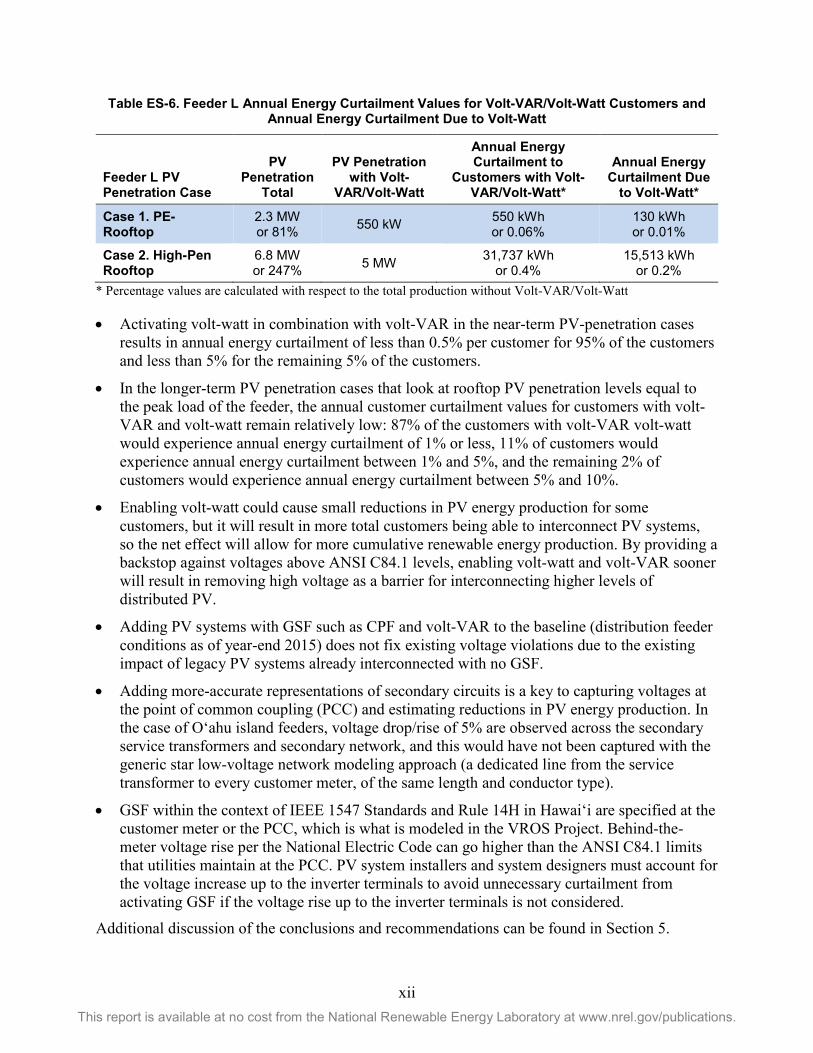
• Activating volt-watt in combination with volt-VAR in the near-term PV-penetration cases—which model all the pending execution interconnection of PV systems with advanced inverters in the two high-penetration feeders included in this study—results in a minor increase in the amount of reductions in PV energy production (0.06–0.5% of annual energy reduction for all pending rooftop PV customers with volt-VAR/volt-watt activated, with 0.01–0.1% attributed to volt-watt as shown in Table ES-5 and Table ES-6). As such, volt-watt is occasionally activated in combination with volt-VAR.
• Activating volt-watt in combination with volt-VAR in the long-term PV-penetration cases—which model a PV penetration of rooftop PV equal to the peak load of the feeder—results in annual energy curtailment values in the range of 0.4–0.9% for all pending rooftop PV customers with volt-VAR/volt-watt activated, with 0.2–0.3% from volt-watt as shown in Table ES-5 and Table ES-6. Volt-watt in the longer term is called upon more frequently. However, the annual energy curtailment values remain very low (less than 0.3% of the total power production without volt-VAR/volt-watt).
Table ES-5. Feeder M34 Annual Energy Curtailment Values for Volt-VAR/Volt-Watt Customers and Annual Energy Curtailment Due to Volt-Watt
Feeder M34 PV Penetration Case
PV Penetration
Total
PV Penetration with Volt-
VAR/Volt-Watt
Annual Energy Curtailment to
Customers with Volt-VAR/Volt-Watt*
Annual Energy Curtailment Due
to Volt-Watt*
Case 1. PE-Rooftop +PE-FIT
10.4 MW or 460% 1.8 MW 11,268 kWh
or 0.5 % 2,576 kWh
or 0.1%
Case 2. High-Pen Rooftop+PE-FIT
14.1 MW or 620% 5.5 MW 73,264 kWh
or 0.9% 24,929 kWh
or 0.3% * Percentage values are calculated with respect to the total production without Volt-VAR/Volt-Watt
xii This report is available at no cost from the National Renewable Energy Laboratory at www.nrel.gov/publications.
Table ES-6. Feeder L Annual Energy Curtailment Values for Volt-VAR/Volt-Watt Customers and Annual Energy Curtailment Due to Volt-Watt
Feeder L PV Penetration Case
PV Penetration
Total
PV Penetration with Volt-
VAR/Volt-Watt
Annual Energy Curtailment to
Customers with Volt-VAR/Volt-Watt*
Annual Energy Curtailment Due
to Volt-Watt*
Case 1. PE-Rooftop
2.3 MW or 81% 550 kW 550 kWh
or 0.06% 130 kWh or 0.01%
Case 2. High-Pen Rooftop
6.8 MW or 247% 5 MW 31,737 kWh
or 0.4% 15,513 kWh
or 0.2% * Percentage values are calculated with respect to the total production without Volt-VAR/Volt-Watt • Activating volt-watt in combination with volt-VAR in the near-term PV-penetration cases
results in annual energy curtailment of less than 0.5% per customer for 95% of the customers and less than 5% for the remaining 5% of the customers.
• In the longer-term PV penetration cases that look at rooftop PV penetration levels equal to the peak load of the feeder, the annual customer curtailment values for customers with volt-VAR and volt-watt remain relatively low: 87% of the customers with volt-VAR volt-watt would experience annual energy curtailment of 1% or less, 11% of customers would experience annual energy curtailment between 1% and 5%, and the remaining 2% of customers would experience annual energy curtailment between 5% and 10%.
• Enabling volt-watt could cause small reductions in PV energy production for some customers, but it will result in more total customers being able to interconnect PV systems, so the net effect will allow for more cumulative renewable energy production. By providing a backstop against voltages above ANSI C84.1 levels, enabling volt-watt and volt-VAR sooner will result in removing high voltage as a barrier for interconnecting higher levels of distributed PV.
• Adding PV systems with GSF such as CPF and volt-VAR to the baseline (distribution feeder conditions as of year-end 2015) does not fix existing voltage violations due to the existing impact of legacy PV systems already interconnected with no GSF.
• Adding more-accurate representations of secondary circuits is a key to capturing voltages at the point of common coupling (PCC) and estimating reductions in PV energy production. In the case of O‘ahu island feeders, voltage drop/rise of 5% are observed across the secondary service transformers and secondary network, and this would have not been captured with the generic star low-voltage network modeling approach (a dedicated line from the service transformer to every customer meter, of the same length and conductor type).
• GSF within the context of IEEE 1547 Standards and Rule 14H in Hawai‘i are specified at the customer meter or the PCC, which is what is modeled in the VROS Project. Behind-the-meter voltage rise per the National Electric Code can go higher than the ANSI C84.1 limits that utilities maintain at the PCC. PV system installers and system designers must account for the voltage increase up to the inverter terminals to avoid unnecessary curtailment from activating GSF if the voltage rise up to the inverter terminals is not considered.
Additional discussion of the conclusions and recommendations can be found in Section 5.

xiii This report is available at no cost from the National Renewable Energy Laboratory at www.nrel.gov/publications.
Some of the caveats to the current work are listed below.
• The current PV systems do not turn off at 1.1 pu voltage as they would in the field according to IEEE 1547. This causes overall higher voltages in the range of the voltage control based grid support functions such as volt-VAR and volt-watt. As such, these functions are called upon more often than they would have if feeder voltages were not as high. Because the VROS project simulated voltages higher than 1.1 pu, the curtailment for PV systems above 1.1 pu was not counted as curtailment associated to a grid support function, however, it is likely that volt-VAR and volt-watt in the simulation were activated more often than it would have been observed in the field.
• Due to the time constraints of the VROS project, the volt-watt algorithm used in combination with CPF and volt-VAR was programmed outside the OpenDSS software. It was observed that in clear-sky days, the volt-watt algorithm used in this project resulted in over-curtailment of up to 10% more of the real power value expected for a 15 min time-step, and over-corrected voltages to the 1.05 pu range in some cases. This implies that the volt-watt annual energy curtailment values are slightly over-estimated. It is suspected that more development is needed in the empirically derived damping factor used in the volt-watt algorithm to improve simulation convergence accuracy.
• Secondary low-voltage voltage networks are added to M34 feeders, but there are no voltage measurements below the service transformers to validate the voltages simulated at the household level. Voltages are validated, however, at the secondary terminals of approximately 10 distribution service transformers with available data from field measurement equipment.
• M34 feeders have no load diversity—that is, the same substation gross load profile drives all the loads represented in the system. During PV system producing hours, the main driver of voltage changes comes from PV systems, not from the load. The metrics quantified in this study (e.g., DeltaV, kWh reduction) mainly are dependent on the voltage profiles during high PV system generation hours, so the limitation is not expected to greatly affect the results. In comparison, Feeder L’s load diversity is captured with implementing advanced metering 15-minute energy usage, and the same conclusions were found.
• Secondary low-voltage circuits are modeled up to the customer meter, but further voltage drop/rise could occur between the meter and the PV system generator terminals. This is consistent with the reference point of applicability where the interconnection and interoperability performance requirements are required to be met. The volt-watt function proposed by the Companies’ initiates reduction in real power when the voltage at the PCC crosses 1.06 pu. Therefore, PV system installers and system designers should account for the additional voltage drop up to the inverter terminals. Note however, that this is a field-installation issue and does not affect the modeling in this report.
• Current PV penetration cases include all PV systems interconnected with the ability to export (as in NEM or customer-grid-supply (CGS) tariffs offered by the Companies’); however, some systems are interconnected in a non-exporting agreement (customer-self-supply (CSS)). The implications of having non-exporting PV-system customers are not modeled in this study and could impact daytime and nighttime voltage profiles.

xiv This report is available at no cost from the National Renewable Energy Laboratory at www.nrel.gov/publications.
• The QSTS was run at 15-minute time steps and, as such, the considerations of impact of GSF to utility LTC operations are relative to the 15-minute time step but might not reflect all of the LTC operations because the load tap changer can regulate voltage at a 30-second resolution. For validation purposes, two days for feeder M34 were run with a 15-second time step, and there were no additional LTC operations observed at the smaller simulation time step as compared to the 15-minute time step results.
• The project did not consider optimizing the current utility voltage-regulating equipment (substation LTC) controls. The LTC in M34 is locked in the simulation when there is reverse power flow at the substation to prevent undervoltages. Yet, the optimal control strategy for the LTCs under high-penetration PV should be further explored. Note that this would only help reduce the impacts to both the customer and the utility.
• The study doesn’t consider other voltage-management solutions (e.g., integrated volt-VAR, decentralized distributed voltage support), and further investigation of the optimal solution for voltage management and how new technologies will integrate with distributed inverter GSF should be conducted.
NREL is supporting Hawaiian Electric in its advanced inverter pilot project. As part of the scope of the advanced inverter pilot project, there is a specific task dedicated to the validation of the VROS Project with field data. The field data will be used to validate the VROS Project models, and in particular to validate the service voltage drop from secondary transformers to the point of interconnection of the PV inverters, as well as the response of multiple inverters in regulating feeder voltage. The updated VROS Project models then will be used to extrapolate from the field data to higher penetration levels of grid-supportive inverters and annual voltage profiles and kWh-production estimates will be updated.
Recently, DOE has designated a new “high impact” phase for the VROS Project – incorporating the project objectives from the advanced inverter pilot. The additional high impact scope includes the evaluation of the impact of customer-sited energy storage, enabling customer electric grid interactive water-heater control, and electric vehicles in the feeder voltage management schemes. For the water-heater control analysis, NREL is leveraging the advanced metering infrastructure (AMI) customer data used in this study to extract occupancy patterns and estimate electric water-heater profiles.
The field data from the advanced inverter pilot project is expected to calibrate and validate the findings of this VROS Project, and the added scope from the “high impact” expansion will address some of the limitations described above (such as the secondary low-voltage networks being modeled up to the PCC and the implications of having non-exporting PV customers with storage).

xv This report is available at no cost from the National Renewable Energy Laboratory at www.nrel.gov/publications.
Table of Contents 1 Introduction ........................................................................................................................................... 1
1.1 Background ................................................................................................................................... 2 1.2 Approach ....................................................................................................................................... 4
2 Feeder Modeling for Time-Series Simulation .................................................................................... 5 2.1 Model Conversion and Steady-State Validation ........................................................................... 5 2.2 Design of Secondary Circuits ........................................................................................................ 8 2.3 Data Processing for Time Series ................................................................................................. 13
2.3.1 Replacing Missing and Outlier Data ............................................................................... 14 2.3.2 Estimating Gross Load in the Feeders ............................................................................ 16 2.3.3 Leveraging AMI Data for Feeder L ................................................................................ 23
2.4 Time Series Model Validation .................................................................................................... 24 2.4.1 Time Series Validation with Grid 2020 Data for M34 ................................................... 24 2.4.2 Time Series Validation with AMI Data for Feeder L ..................................................... 25 2.4.3 Preliminary Evaluation of Current LTC Operations ....................................................... 31
2.5 Final 2015 Baseline Feeder Models ............................................................................................ 31 3 Time-Series Simulation and Modeling of Advanced Inverter Modes ............................................ 34
3.1 PV Systems—Assumptions and Advanced Inverter Modes ....................................................... 34 3.2 Implementation of Inverter Controls in OpenDSS ...................................................................... 36 3.3 Time-Series Simulation with Advanced Inverters ...................................................................... 38
4 Results—Voltage Operating Strategies with Advanced Inverters ................................................. 40 4.1 Photovoltaic Penetration Cases and Metrics ............................................................................... 40 4.2 M34 Feeders Results ................................................................................................................... 43
4.2.1 Voltage Profiles and DeltaV Metric ................................................................................ 43 4.2.2 Utility and Customer Implications for 0.95 CPF and Volt-VAR Modes ........................ 52 4.2.3 Utility and Customer Implications for 0.95 CPF/Volt-Watt and Volt-VAR/
Volt-Watt Modes ............................................................................................................ 59 4.3 Feeder L Results .......................................................................................................................... 60
4.3.1 Voltage Profiles and DeltaV Metric ................................................................................ 60 4.3.2 Utility and Customer Implications with 0.95 CPF and Volt-VAR ................................. 66 4.3.3 Utility and Customer Implications with 0.95 CPF/Volt-Watt and Volt-VAR/
Volt-Watt ........................................................................................................................ 71 4.4 Annual Energy Reduction to Customers and Impact to the Bulk System ................................... 71 4.5 Difference in Effectiveness for Advanced Inverter Functions in M34 and L Feeders ................ 77 4.6 Importance of Reactive Power Priority Implementation ............................................................. 79
5 Summary of Conclusions and Recommendations.......................................................................... 80 6 Future Work ......................................................................................................................................... 83 References ................................................................................................................................................. 85 Appendix A. Model Conversion and Validation Data ............................................................................ 86
Conversion from Synergi to OpenDSS ................................................................................................ 86 Time-Series Validation ......................................................................................................................... 87
Appendix B. Simulation Results Plots .................................................................................................... 93 M34 Case 1 Voltage Profiles for CPF 0.95/Volt-Watt and Volt-VAR/Volt-Watt ............................... 93 M34 Case 1. PE-Rooftop+PE-FIT Utility and Customer Implications for CPF 0.95 and
Volt-VAR .................................................................................................................................... 94 Feeder L Case 1. PE-Rooftop Voltage Profiles for CPF 0.95/Volt-Watt and Volt-VAR/
Volt-Watt ..................................................................................................................................... 96
xvi This report is available at no cost from the National Renewable Energy Laboratory at www.nrel.gov/publications.
List of Figures Figure ES-1. Advanced inverter mode settings for volt-VAR, and volt-watt. ........................................... viii Figure 1. Geographical view of K3L distribution feeders in Synergi and OpenDSS ................................... 6 Figure 2. Geographical view of M34 distribution feeders in Synergi and OpenDSS ................................... 7 Figure 3. Percentage error of voltage (left) and sequence impedance (right) with respect to distance from
the feeder head for K3L feeders ............................................................................................... 7 Figure 4. Percentage error of voltage (left) and sequence impedance (right) with respect to distance from
the feeder head for M34 feeders............................................................................................... 8 Figure 5. Diagram showing the load model provided by Hawaiian Electric on the left, and the detailed
load transformer and secondary circuit being added by NREL to the existing model for every load node .................................................................................................................................. 9
Figure 6. Customer load nodes overlaid on GIS land-use database for M3 and M4 loads ......................... 10 Figure 7. Customer load nodes overlaid on GIS land-use database for the K region loads ........................ 11 Figure 8. Flowchart showing the methodology to assign a secondary design process to OH and UG
residential customers from a total of 55 detailed secondary designs provided by Hawaiian Electric ................................................................................................................................... 13
Figure 9. Linear Regression between M3 and M4 circuit load. .................................................................. 14 Figure 10. M3 outlier data-replacement example with M4 data ................................................................. 15 Figure 11. Nightime M3 and M4 power factors for 2015 ........................................................................... 16 Figure 12. Nighttime real versus reactive power regression for M34 circuits using M3 reactive power data
for both ................................................................................................................................... 17 Figure 13. The MWh/MW values versus irradiance for a fleet of PV systems in the M34 region ............. 18 Figure 14. The M3 real power and PV system production estimates produced using the PQ regression
method versus the MWh/MW method ................................................................................... 18 Figure 15. The M4 real power and PV-production estimates using the PQ regression method versus the
MWh/MW method ................................................................................................................. 19 Figure 16. M34 Substation gross real power estimates from MWh/MW and PQ regression methods
compared to 2015 and 2008 substation net load profiles (top—real power; bottom—scaled and normalized) ...................................................................................................................... 20
Figure 17. The K3L substation gross real power estimates from MWh/MW and PQ regression methods compared to 2015 and 2012 substation net load profiles ....................................................... 20
Figure 18. The K3 gross real power from the MWh/MW method and PV system profiles ....................... 21 Figure 19. The L feeder gross real power from the MWh/MW method and PV system profiles ............... 21 Figure 20. Flowchart summarizing the data processing of load and PV energy for M34 feeders .............. 22 Figure 21. Flowchart summarizing the data processing of load and PV energy for K3L region feeders ... 23 Figure 22. Feeder L circuit 15-min SCADA data compared to the aggregate AMI customer meters; the
comparison reflects that there is approximately 1 MW of demand that is not metered via AMI (the x-axis represents time in 15-min interval for a year). ............................................ 24
Figure 23. Real power and voltage Grid 20/20 measurements (blue) at 4 service transformer locations compared to OpenDSS simulation results (red) ..................................................................... 26
Figure 24. Real power and voltage Grid 20/20 measurements (blue) at 4 service transformer locations compared to OpenDSS simulation results (red) ..................................................................... 27
Figure 25. Envelope of maximum and minimum voltages for simulated load (top) and measured AMI loads (bottom) for all customer loads in feeder L. ................................................................. 28
Figure 26. Envelope of maximum and minimum voltage across the secondary circuit of a service transformer location in which maximum and minimum simulated (top) and measured (bottom) voltage envelopes match well. ................................................................................ 29
Figure 27. Envelope of maximum and minimum voltage across the secondary circuit of two service transformer locations (top: underestimation, bottom: overestimation). ................................. 30
Figure 28. June 9, 2015, highest (left) and lowest (right) voltage heat map for M3 and M4 feeders ......... 32

xvii This report is available at no cost from the National Renewable Energy Laboratory at www.nrel.gov/publications.
Figure 29. Voltage to distance from the substation plot of primary voltages (solid lines) and secondary voltages (dotted lines) for M3 and M4 feeders on June 9 at 11:15 a.m. ................................ 33
Figure 30. May 23, 2015, highest (left) and lowest (right) voltage heat map for feeder L ......................... 33 Figure 31. Voltage to distance from the substation plot of primary voltages (solid lines) and secondary
voltages (dotted lines) for feeder L on May 23 at 12:30 p.m. ................................................ 34 Figure 32. Advanced inverter mode settings for constant power factor, volt-VAR, and volt-watt ............ 36 Figure 33. Voltages at every customer meter in M34 feeders for the highest-voltage week of the year for
Case 0 ..................................................................................................................................... 44 Figure 34. Voltages at every customer meter for M34 feeders for the highest-voltage week of the year for
Case 0.AI ................................................................................................................................ 44 Figure 35. Case 1. PE-Rooftop (left) and Case 1. PE-Rooftop+PE-FIT (right) customer meter voltages for
M34 feeders for the highest-voltage week of the year with no advanced inverters ............... 45 Figure 36. Case 1. PE-Rooftop (left) and Case 1. PE-Rooftop+PE-FIT (right) customer meter voltages for
M34 feeders for the highest-voltage week of the year with 1.8 MW of the total PV systems with 0.95 CPF activated ......................................................................................................... 46
Figure 37. Case 1. PE-Rooftop (left) and Case 1. PE-Rooftop+PE-FIT (right) customer meter voltages for M34 feeders for the highest-voltage week of the year with 1.8 MW of the total PV systems with Volt-VAR activated ....................................................................................................... 46
Figure 38. Case 2. High-Pen Rooftop (left) and Case 2. High-Pen Rooftop+PE-FIT (right) customer meter voltages for M34 feeders for the highest-voltage week of the year with no advanced inverters ................................................................................................................................................ 48
Figure 39. Case 2. High-Pen Rooftop (left) and Case 2. High-Pen Rooftop+PE-FIT (right) customer meter voltages for M34 feeders for the highest-voltage week of the year with 0.95 CPF activated in 5.5 MW of rooftop PV energy ............................................................................................... 49
Figure 40. Case 2. High-Pen Rooftop (left) and Case 2. High-Pen Rooftop+PE-FIT (right) customer meter voltages for M34 feeders for the highest-voltage week of the year with volt-VAR activated in 5.5 MW of rooftop PV systems ......................................................................................... 49
Figure 41. Case 2. High-Pen Rooftop (left) and Case 2. High-Pen Rooftop+PE-FIT (right) customer meter voltages for M34 feeders for the highest-voltage week of the year with 0.95 CPF/volt-watt activated in 5.5 MW of rooftop PV systems .......................................................................... 51
Figure 42. Case 2. High-Pen Rooftop (left) and Case 2. High-Pen Rooftop+PE-FIT (right) customer meter voltages for M34 feeders for the highest-voltage week of the year with volt-VAR/volt-watt activated in 5.5 MW of rooftop PV systems .......................................................................... 51
Figure 43. Feeder head real and reactive power (top) and aggregate real and reactive power production for all PV systems modeled (bottom) for Case 1. PE-Rooftop with 1.8-MW PV systems interconnected at CPF 0.95, compared to Case 1. PE-Rooftop without advanced inverters; the grey-shaded areas represent the difference in reactive power demand at the feeder head (top) and absorption from the PV systems with 0.95 CPF (bottom); the orange-shaded area illustrates the amount of curtailed energy from activating 0.95 CPF in the pending rooftop PV systems ............................................................................................................................. 53
Figure 44. Feeder head real and reactive power (top) and aggregate real and reactive power production for all PV systems modeled (bottom) for Case 1. PE-Rooftop with 1.8 MW PV in volt-VAR mode, compared to Case 1. PE-Rooftop without advanced inverters; the grey-shaded areas represent the difference in reactive power demand at the feeder head (top) and absorption from the PV systems with volt-VAR (bottom); the orange-shaded area illustrates the amount of curtailed energy from activating volt-VAR in the pending rooftop PV systems ............... 54
Figure 45. Top: Substation LTC tap positions for Case 1. PE-Rooftop with 1.8 MW in 0.95 CPF mode and cumulative number of tap changes as compared to Case 1. PE-Rooftop with no advanced inverters for 2 days in the highest-voltage week of the year; bottom: overvoltages (red) and undervoltages (blue) time-series voltage violations for Case 1. PE-Rooftop with 1.8 MW in

xviii This report is available at no cost from the National Renewable Energy Laboratory at www.nrel.gov/publications.
0.95 CPF mode, and cumulative number of voltage violations (solid black) compared to Case 1. PE-Rooftop with no advanced inverters (black dotted)............................................. 55
Figure 46. Top: Substation LTC tap positions for Case 1. PE-Rooftop with 1.8 MW in volt-VAR mode and cumulative number of tap changes compared to Case 1. PE-Rooftop with no advanced inverters for two days in the highest-voltage week of the year; bottom: overvoltage (red) and undervoltage (blue) time-series voltage violations for Case 1. PE-Rooftop with 1.8 MW in volt-VAR mode, and cumulative number of voltage violations (solid black) compared to Case 1. PE-Rooftop with no advanced inverters (black dotted)............................................. 56
Figure 47. Feeder head real and reactive power (top) and aggregate real and reactive power production for all PV systems modeled (bottom) for Case 2. High-Pen Rooftop with 5.5 MW PV interconnected at CPF 0.95, compared to Case 2. High-Pen Rooftop with 5.5 MW with volt-VAR; the grey-shaded areas represent the difference in reactive power demand at the feeder head (top) and absorption from the PV systems with volt-VAR and 0.95 CPF (bottom); the orange-shaded area illustrates the amount of curtailed energy from activating 0.95 CPF versus volt-VAR in the pending rooftop PV systems ............................................................ 58
Figure 48. Top: Substation LTC tap positions for Case 2. High-Pen Rooftop with 5.5 MW in 0.95 CPF mode and cumulative number of tap changes compared to Case 2. High-Pen Rooftop with volt-VAR for two days in the highest-voltage week of the year; bottom: Overvoltage (red) and undervoltage (blue) time-series voltage violations for Case 2. High-Pen Rooftop with 5.5 MW in 0.95 CPF mode, and cumulative number of voltage violations (solid black) compared to Case 1. PE-Rooftop with volt-VAR (black dotted) ........................................... 59
Figure 49. Voltages at every customer meter in feeder L for the highest-voltage week of the year for Case 0 .............................................................................................................................................. 61
Figure 50. Voltages at every customer meter in feeder L for the highest-voltage week of the year for Case 1. PE-Rooftop with no advanced inverters............................................................................. 62
Figure 51. Voltages at every customer meter in feeder L for the highest-voltage week of the year for Case 1. PE-Rooftop with CPF 0.95 (left) and volt-VAR (right) activated on 550 kW of PV systems ................................................................................................................................... 63
Figure 52. Voltages at every customer meter in feeder L for the highest-voltage week of the year for Case 2. High-Pen Rooftop .............................................................................................................. 64
Figure 53. Voltages at every customer meter in feeder L for the highest-voltage week of the year for Case 2. High-Pen Rooftop with CPF 0.95 (left) and volt-VAR (right) activated on 550 kW of PV energy ............................................................................................................................... 65
Figure 54. Voltages at every customer meter in feeder L for the highest-voltage week of the year for Case 2. High-Pen Rooftop with CPF 0.95/volt-watt (left) and volt-VAR/volt-watt (right) activated on 5 MW of PV systems ........................................................................................................ 66
Figure 55. Feeder head real and reactive power (top) and aggregate real and reactive power production for all PVs modeled (bottom) for Case 1. PE-Rooftop with 550-kW PV systems interconnected at CPF 0.95, as compared to Case 1. PE-Rooftop with 550-kW with volt-VAR; the grey-shaded areas represent the difference in reactive power demand at the feeder head (top) and absorption from the PV systems with volt-VAR and 0.95 CPF (bottom); the orange-shaded area illustrates the amount of curtailed energy from activating 0.95 CPF versus volt-VAR in the pending rooftop PV systems ............................................................................................ 67
Figure 56. Top: Substation LTC tap positions for Case 1. PE-Rooftop with 550 kW in 0.95 CPF mode and cumulative number of tap changes compared to Case 1. PE-Rooftop with volt-VAR for two days in the highest-voltage week of the year; bottom: overvoltage (red) and undervoltage (blue) time-series voltage violations for Case 1. PE-Rooftop with 550 kW in 0.95 CPF mode, and cumulative number of voltage violations (solid black) compared to Case 1. PE-Rooftop with volt-VAR (black dotted) ................................................................................................ 68
Figure 57. Feeder head real and reactive power (top) and aggregate real and reactive power production for all PVs modeled (bottom) for Case 2. High-Pen Rooftop with 5 MW PV systems

xix This report is available at no cost from the National Renewable Energy Laboratory at www.nrel.gov/publications.
interconnected at CPF 0.95, as compared to Case 2. High-Pen Rooftop with 5 MW with volt-VAR; the grey-shaded areas represent the difference in reactive power demand at the feeder head (top) and absorption from the PV systems with volt-VAR and 0.95 CPF (bottom); the orange-shaded area illustrates the amount of curtailed energy from activating 0.95 CPF versus volt-VAR in the added rooftop PV systems................................................................ 69
Figure 58. Top: Substation LTC tap positions for Case 2. High-Pen Rooftop with 5 MW in 0.95 CPF mode and cumulative number of tap changes as compared to Case 2. High-Pen Rooftop with volt-VAR for two days in the highest-voltage week of the year; bottom: overvoltage (red) and undervoltage (blue) time-series voltage violations for Case 2. High-Pen Rooftop with 5 MW in 0.95 CPF mode, and cumulative number of voltage violations (solid black) as compared to Case 2. High-Pen Rooftop with volt-VAR (black dotted) ................................ 70
Figure 59. Histogram of percent of annual energy curtailed for every customer with volt-VAR/volt-watt activated for M34 Case 1. PE-Rooftop+PE-FIT (left) and feeder L Case 1. PE-Rooftop (right) ..................................................................................................................................... 75
Figure 60. Histogram of percent of annual energy curtailed for every customer with volt-VAR/volt-watt activated (left) for M34 Case 2. High-Pen Rooftop+PE-FIT, and feeder L Case 2. High-Pen Rooftop (right) ....................................................................................................................... 76
Figure 61. Ratio of secondary transformer capacity in kVA to number of customers or all transformers in the overhead rural area of feeders M34; each tick on the x-axis is an aggregate load node or secondary transformer ............................................................................................................ 77
Figure 62. Ratio of secondary transformer capacity kVA to number of customers for all transformers in the overhead suburban area of feeder L; each tick on the x-axis is an aggregate load node or secondary transformer ............................................................................................................ 78
Figure 63. M4 Rural overhead secondary example with three PV systems for Case 2. High-Pen Rooftop; red indicates no advanced inverters and blue indicates volt-VAR ......................................... 78
Figure 64. Feeder L suburban overhead secondary example with 9 PV systems with advanced inverter capabilities (yellow) and 1 legacy (red) for Case 2. High-Pen Rooftop; red indicates no advanced inverters and blue indicates volt-VAR; note that, for clarity of the image, the PV systems are only shown in the blue secondary with volt-VAR but both scenarios in the figure have the same 10 PV systems in the model ........................................................................... 79
Figure 65. Case 1. PE-Rooftop with 1.8 MW of pending rooftop PV systems in volt-VAR VAR priority mode (left) and volt-VAR watt priority mode (right) ............................................................ 80
Figure 66. Diagrammatic view of Synergi to OpenDSS model conversion depicting the syntax identification process ............................................................................................................. 86
Figure 67 . Power (top) and voltage (bottom) time-series comparison between Grid 20/20 measurements and OpenDSS model at M3 transformer 1400 for September 16–17, 2015 .......................... 88
Figure 68. Power (top) and voltage (bottom) time-series comparison between Grid 20/20 measurements and OpenDSS model at M3 transformer 1413 for September 16–17, 2015 .......................... 88
Figure 69. Power (top) and voltage (bottom) time-series comparison between Grid 20/20 measurements and OpenDSS model at M4 transformer 1403 for September 16–17, 2015 .......................... 89
Figure 70. Power (top) and voltage (bottom) time-series comparison between Grid 20/20 measurements and OpenDSS model at M4 transformer 1404 for September 16–17, 2015 .......................... 89
Figure 71. Power (top) and voltage (bottom) time-series comparison between Grid 20/20 measurements and OpenDSS model at M4 transformer 1414 for September 16–17, 2015 .......................... 90
Figure 72. Power (top) and voltage (bottom) time-series comparison between Grid 20/20 measurements and OpenDSS model at M4 transformer 1579 for September 16–17, 2015 .......................... 90
Figure 73. Power (top) and voltage (bottom) time-series comparison between Grid 20/20 measurements and OpenDSS model at M4 transformer 1585 for September 16–17, 2015 .......................... 91
Figure 74. Power (top) and voltage (bottom) time-series comparison between Grid 20/20 measurements and OpenDSS model at M4 transformer 1586 for September 16–17, 2015 .......................... 91

xx This report is available at no cost from the National Renewable Energy Laboratory at www.nrel.gov/publications.
Figure 75. Power (top) and voltage (bottom) time-series comparison between Grid 20/20 measurements and OpenDSS model at M4 transformer 1587 for September 16–17, 2015 .......................... 92
Figure 76. Case 1. PE-Rooftop CPF 0.95/volt-watt (left) and volt-VAR/volt-watt (right) customer meter voltages for M34 feeders for the highest-voltage week of the year with no advanced inverters ................................................................................................................................................ 93
Figure 77. Case 1. PE-Rooftop+PE-FIT CPF 0.95/volt-watt (left) and volt-VAR/volt-watt (right) customer meter voltages for M34 feeders for the highest-voltage week of the year with no advanced inverters .................................................................................................................. 93
Figure 78. (1) Feeder head real and reactive power; (2) aggregate real and reactive power production for all PV systems modeled for Case 1. PE-Rooftop+PE-FIT with 1.8 MW PV systems interconnected at CPF 0.95, compared to Case 1. PE-Rooftop+PE-FIT without advanced inverters; (3) substation LTC tap positions for Case 1. PE-Rooftop+PE-FIT with 1.8 MW in 0.95 CPF mode and cumulative number of tap changes compared to Case 1. PE-Rooftop+PE-FIT with no advanced inverters for 2 days in the highest-voltage week of the year; and (4) overvoltages (red) and undervoltages (blue) time-series voltage violations for Case 1. PE-Rooftop+PE-FIT with 1.8 MW in 0.95 CPF mode, and cumulative number of voltage violations (solid black) compared to Case 1. PE-Rooftop+PE-FIT with no advanced inverters (black dotted) .......................................................................................................... 94
Figure 79. (1) Feeder head real and reactive power; (2) aggregate real and reactive power production for all PV systems modeled for Case 1. PE-Rooftop+PE-FIT with 1.8 MW PV systems interconnected at volt-VAR, compared to Case 1. PE-Rooftop+PE-FIT without advanced inverters; (3) substation LTC tap positions for Case 1. PE-Rooftop+PE-FIT with 1.8 MW in volt-VAR mode and cumulative number of tap changes compared to Case 1. PE-Rooftop+PE-FIT with no advanced inverters for 2 days in the highest-voltage week of the year; and (4) overvoltages (red) and undervoltages (blue) time-series voltage violations for Case 1. PE-Rooftop+PE-FIT with 1.8 MW in volt-VAR mode, and cumulative number of voltage violations (solid black) compared to Case 1. PE-Rooftop+PE-FIT with no advanced inverters (black dotted) .......................................................................................................... 95
Figure 80. Case 1. PE-Rooftop CPF 0.95/volt-watt (left) and volt-VAR/volt-watt (right) customer meter voltages for feeder L for the highest-voltage week of the year with no advanced inverters .. 96
List of Tables Table ES-1. Volt-VAR Settings ................................................................................................................. viii Table ES-2. Volt-Watt Settings ................................................................................................................. viii Table ES-3. Summary Metrics of Four PV Penetration Cases for M34 Feeders with CPF 0.95/Volt-Watt
and Volt-VAR/Volt-Watt in New Rooftop PV ........................................................................ x Table ES-4. Summary Metrics of Four PV Penetration Cases for Feeder L with CPF 0.95/Volt-Watt and
Volt-VAR/Volt-Watt in New Rooftop PV ............................................................................... x Table ES-5. Feeder M34 Annual Energy Curtailment Values for Volt-VAR/Volt-Watt Customers and
Annual Energy Curtailment Due to Volt-Watt ....................................................................... xi Table ES-6. Feeder L Annual Energy Curtailment Values for Volt-VAR/Volt-Watt Customers and
Annual Energy Curtailment Due to Volt-Watt ...................................................................... xii Table 1. Secondary Circuit Designs for Each Customer Type ................................................................... 12 Table 2. Load Classification to Map Each Aggregate Load Node Provided by Hawaiian Electric to a
Secondary Design .................................................................................................................. 12 Table 3. M34 and L General Feeder Characteristics ................................................................................... 31 Table 4. M34 Feeders PV Penetration Cases .............................................................................................. 41 Table 5. Feeder L PV Penetration Cases ..................................................................................................... 42 Table 6. DeltaV (10 a.m. to 2 p.m.) for the Highest Voltage Week of the Year: Case 1. PE-Rooftop and
Case 1. PE-Rooftop+PE-FIT with 0.95 CPF and Volt-VAR ................................................. 47

xxi This report is available at no cost from the National Renewable Energy Laboratory at www.nrel.gov/publications.
Table 7. DeltaV (10 a.m. to 2 p.m.) for the Highest Voltage Week of the Year: Case 1. PE-Rooftop and Case 1. PE-Rooftop+PE-FIT with 0.95 CPF/Volt-Watt and Volt-VAR/Volt-Watt .............. 48
Table 8. DeltaV (10 a.m. to 2 p.m.) for the Highest-Voltage Week of the Year: Case 2. High-Pen Rooftop and Case 2. High-Pen Rooftop+PE-FIT with 0.95 CPF and Volt-VAR ................................ 50
Table 9. DeltaV (10 a.m. to 2 p.m.) for the Highest-Voltage Week of the Year: Case 2. High-Pen Rooftop and Case 2. High-Pen Rooftop+PE-FIT with 0.95 CPF/Volt-Watt and Volt-VAR/Volt-Watt ................................................................................................................................................ 52
Table 10. Case 1. PE Rooftop and Case 1. PE-Rooftop+PE-FIT kWh Curtailment and kVAR Demand Increase from CPF 0.95 and Volt-VAR Activated in 1.8 MW Rooftop PV Systems for the Highest-Voltage Week of the Year ........................................................................................ 57
Table 11. Case 2. High-Pen Rooftop and Case 2. High-Pen Rooftop+PE-FIT kWh Curtailment and kVAR Demand Increase from CPF 0.95 and Volt-VAR Activated in 5.5 MW Rooftop PV Energy for the Highest-Voltage Week of the Year ............................................................................ 59
Table 12. Case 2. High-Pen Rooftop and Case 2. High-Pen Rooftop+PE-FIT kWh Curtailment and kVAR Demand Increase from CPF 0.95/Volt-Watt and Volt-VAR/Volt-Watt Activated in 5.5 MW Rooftop PV Systems for the Highest-Voltage Week of the Year .......................................... 60
Table 13. DeltaV (10 a.m. to 2 p.m.) for the Highest-Voltage Week of the Year: Case 1. PE-Rooftop with 0.95 CPF and Volt-VAR ........................................................................................................ 63
Table 14. DeltaV (10 a.m. to 2 p.m.) for the Highest-Voltage Week of the Year: Case 1. PE-Rooftop with 0.95 CPF and Volt-VAR ........................................................................................................ 64
Table 15. DeltaV (10 a.m. to 2 p.m.) for the Highest-Voltage Week of the Year: Case 2. High-Pen Rooftop with 0.95 CPF and Volt-VAR .................................................................................. 65
Table 16. DeltaV (10 a.m. to 2 p.m.) for the Highest-Voltage Week of the Year: Case 2. High-Pen Rooftop with 0.95 CPF/Volt-Watt and Volt-VAR/Volt-Watt ............................................... 66
Table 17. Case 1. PE Rooftop Kilowatt-Hour Curtailment and kVAR Demand Increase from CPF 0.95 and Volt-VAR Activated in 550-kW Rooftop PV Systems for the Highest-Voltage Week of the Year .................................................................................................................................. 68
Table 18. Case 2. High-Pen Rooftop Kilowatt-Hour Curtailment and kVAR Demand Increase from CPF 0.95 and Volt-VAR Activated in 5-MW Rooftop PV Systems for the Highest-Voltage Week of the Year ................................................................................................................... 70
Table 19. Case 1. PE Rooftop Kilowatt-Hour Curtailment and kVAR Demand Increase from CPF 0.95/Volt-Watt and Volt-VAR/Volt-Watt activated in 550-kW rooftop PV Systems for the Highest-Voltage Week of the Year ........................................................................................ 71
Table 20. Case 2. High-Pen Rooftop Kilowatt-Hour Curtailment and kVAR Demand Increase from CPF 0.95/Volt-Watt and Volt-VAR/Volt-Watt Activated in 5-MW Rooftop PV Systems for the Highest-Voltage Week of the Year .................................................................................. 71
Table 21. M34 Annual Kilowatt-Hour Curtailment and kVAR Demand Increase for CPF 0.95/Volt-Watt and Volt-VAR/Volt-Watt ....................................................................................................... 72
Table 22. Feeder L Annual Kilowatt-Hour Curtailment and kVAR Demand Increase for CPF 0.95/Volt-Watt and Volt-VAR/Volt-Watt .............................................................................................. 73
Table 23. Feeder M34 Annual Energy Curtailment Values for Volt-VAR/Volt-Watt Customers and Proportion of that Curtailment Due to Volt-Watt .................................................................. 73
Table 24. Feeder L Annual Energy Curtailment Values for Volt-VAR/Volt-Watt Customers and Proportion of that Curtailment Due to Volt-Watt .................................................................. 74

1 This report is available at no cost from the National Renewable Energy Laboratory at www.nrel.gov/publications.
1 Introduction The Hawaiian Electric Companies, in collaboration with the Smart Inverter Technical Working Group Hawai‘i (SITWG), have partnered with the U.S Department of Energy’s National Renewable Energy Laboratory (NREL) to evaluate and recommend the implementation of advanced inverter voltage-regulation grid support functions (GSF) for solar photovoltaic (PV) systems and installations to improve the interconnection of distributed energy resources (DER) in Hawai‘i.
For this Voltage Regulation Operational Strategies (VROS) Project, NREL conducted quasi-static time-series (QSTS) simulations and scenario analyses on two O‘ahu feeders with a high penetration of legacy rooftop net energy metering (NEM) and feed-in tariff (FIT) solar PV systems (penetration levels of 64% and 150% gross daytime minimum loads), to understand the effectiveness of the voltage-regulation GSF which are not presently covered in IEEE 1547-2003. The QSTS simulations characterized the locational energy curtailment impacts to PV-system customers and the relative locational benefits to utility feeder operations of several advanced inverter-voltage regulation grid support functions under consideration by the Hawaiian Electric Companies. The advanced inverter voltage-regulation GSF modeled are: (1) Constant power factor (CPF) of 0.95, (2) volt-VAR, (3) CPF of 0.95 in combination with volt-watt, and (4) volt-VAR in combination with volt-watt.
The Hawaiian Electric Companies and NREL collaborated with the members of the SITWG throughout the project to achieve a recommended approach for this study. The SITWG consists of members from the PV-inverter manufacturing industry, planners, and engineers from California utilities with interest and expertise in grid integration of PV inverters and systems. Hawaiian Electric, NREL, and members of the SITWG designed the scope of work to address some of the following research questions.
1. Which advanced inverter function is more effective in regulating voltage (e.g., maintaining voltage within power quality limits, minimizing voltage variation)?
2. What is the relative impact of the advanced inverter voltage-regulation functions to customer-sited PV system kilowatt-hour (kWh) reduction?
3. What is the relative impact of advanced inverter voltage-regulation functions in overall feeder reactive power demand?
4. Is active or reactive power priority the right implementation for Hawai‘i and overall voltage performance?
These four questions are answered through modeling and simulation of two O‘ahu substations with several scenarios of advanced inverter PV-penetration growth using QSTS power-flow simulation. The VROS project is successful in that it identified technical recommendations for the activation of voltage-regulation GSF that addresses Hawai‘i’s unique feeder characteristics and operations with the least energy curtailment impact to PV-system customers.

2 This report is available at no cost from the National Renewable Energy Laboratory at www.nrel.gov/publications.
1.1 Background This VROS Project follows a previous effort in which the Hawaiian Electric Companies worked with NREL to develop and conduct a test plan for advanced inverter PV functions, and to characterize how the tested advanced functionalities performed in an environment that represents the dynamics of O‘ahu’s electrical distribution system [1]-[3].
In collaboration with the members of the SITWG, the Hawaiian Electric Companies identified a need to expand the laboratory testing mentioned above to perform modeling and simulation of feeder operations with solar PV system advanced inverters over a longer (year-long) period. The key concern expressed by the members of the SITWG was that the activation of voltage-regulation GSF—especially volt-VAR with reactive power priority and the volt-watt function—would have significant curtailment to the PV-system customer.
The prior advanced inverter baseline hardware performance testing and the dynamic power hardware-in-the-loop (PHIL) tests addressed impacts to the utility and the PV customer in very short (cycles to minutes) time horizons that are studied in a laboratory-testing environment. The PHIL tests simulated the same two O‘ahu island distribution circuits used in this VROS Project. Due to the computational speed limitations of the PHIL system, a reduced-order model of each distribution feeder is developed and used for the PHIL tests [2]. Volt-VAR control is added to the project scope by NREL, but only for the baseline hardware testing. The majority of the PHIL tests focused on various combinations of CPF and volt-watt autonomous control. This work found the voltage regulation functions to be reliable and beneficial to distribution feeder operations, and did not identify any undesired dynamic interactions. Because this work examined short periods, it did not quantify the impact of the functions on annual energy production from distributed PV systems, nor did it examine benefits to distribution-system operations that accrue over longer time scales.
Similar inquiries have been posed in the past by the research led by the Electric Power Institute (EPRI) in collaboration with the California Public Utility Commission, Sandia National Laboratories, and NREL in terms of determining the effectiveness and grid impact of advanced inverters [4]. Some of assumptions of the EPRI California Solar Initiative (CSI) study, however, are not applicable to the characteristics of the distribution grid and PV-deployment scenarios seen in Hawai‘i. Some of these observations are described below.
• Hawaiian Electric Companies feeder voltage regulation scheme (primarily with load tap changers (LTCs)) is different than the California Utilities feeders analyzed in prior studies (LTCs, line regulators, and capacitor banks).
• The CSI study assumed that there is a 10% excess capacity available from installed PV system to provide volt-ampere reactive (VAR) support.
• CA Rule 21 and the existing draft of Rule 21 specify a “watt priority” mode of operation for grid support functions.
Hawai’i has a very high penetration of legacy inverters and rooftop PV systems in the nominal 10-kW size range. These rooftop PV inverters typically are undersized with respect to the rating of the PV cells. Also, the rooftop PV systems mostly are located in secondary circuits that are approximate using a start network design (one dedicated line from the service transformer to the

3 This report is available at no cost from the National Renewable Energy Laboratory at www.nrel.gov/publications.
customer of same length and conductor type) in the EPRI CSI study. The key factors that drove the decision to conduct this Hawai‘i -specific research to confirm the benefits and impacts of activating the voltage regulation GSF are differences in the type, size, and location of installed PV systems; the feeder characteristics and voltage operational scheme differences; and Hawaiian Electric’s reactive power priority implementation of grid support functions.
The recently published EPRI report for the Arizona Public Service (APS) Solar Partner Program (SPP) describes the field-testing results for a variety of grid support functions [5]. The field-testing strategy used is a day-on/day-off comparison of advanced inverter modes on six research feeders and was performed in the summer and fall of 2016. The inverters operated in a VAR priority mode, yet there was little observable impact on the total PV real power production during summer and early fall months. Advanced inverters observed under the APS SPP did not frequently experience curtailment due to a relatively modest DC/AC ratio of 1.1, as well as thermal degradation. This study proposes evaluating a more aggressive DC/AC ratio of 1.2 and whether energy curtailment from implementing VAR priority grid support functions is an upcoming concern. Other conclusions and recommendations of the APS SPP project are listed below [5].
• Primary feeder voltage showed little noticeable effect—even with the most aggressive advanced inverter settings—based on penetration levels on the research feeders.
• Hosting capacity can be improved with advanced inverters, but results depend on circuit construction, loading, and number of participating PV systems. In certain cases, a full retrofit (or another solution) might be necessary to resolve voltage issues.
• VAR priority is preferred for grid applications, but has not been implemented in the first U.S. advanced/smart inverter standard (i.e., CA Rule 21).
• General voltage issues were best mitigated at the customer level using a configuration based on volt-VAR.
Previous work by NREL with San Diego Gas and Electric (SDG&E) looked at modeling of volt-VAR and fixed power factor, however, load and PV systems were represented at the aggregate level at the primary of the service transformers [6]. The study also considered oversize inverters, watt priority, and volt-VAR support during non-PV-producing hours. The study concluded that smart PV inverters installed in sufficient quantity at the right location can impact a distribution circuit voltage by providing reactive power support with the inverter operating at fixed power factor settings or in volt-VAR mode. Lastly, SolarCity and NREL looked at the estimated impact of PV systems with volt-VAR control on voltage-reduction energy savings and distribution system power quality on two utility feeders (one Hawaiian Electric and one Pacific General Electric), and concluded that voltage-reduction energy savings increased with volt-VAR control, and that they also had a positive impact on the power quality [7]. This work included a star network approximation for the Hawaiian Electric feeder for secondary low-voltage circuits.
Although many research projects—including those mentioned above—have examined distributed inverter-based voltage support functions from many different angles, activation of these functions in the field by U.S. utilities largely has been limited to pilot studies. Hawaiian Electric has required distributed PV inverters to operate at 0.95 CPF since early 2016, but no other U.S. utility is known to have required any of the three functions examined here on a

4 This report is available at no cost from the National Renewable Energy Laboratory at www.nrel.gov/publications.
system-wide level. In fact, the current U.S. interconnection standard, IEEE 1547-2003 [8] prohibits DERs from actively regulating voltage (exceptions to the standard can be made with the agreement of the utility and the PV owner, but such exceptions are very rare). In recognition of the fact that DER-based voltage support is needed at higher penetration levels, both California and Hawai‘i have published interconnection rules requiring various grid support functions starting in September 2017. California’s Rule 21 requires only volt-VAR and CPF capability, and with significantly different parameters than Hawai‘i’s Source Requirement Document (SRD). Most importantly, Rule 21 calls for volt-VAR with real power priority, whereas Hawaiian Electric calls for reactive power priority, which will ensure that reactive power is available when it is most needed. Additionally, California does not call for volt-watt capability, whereas Hawai‘i does.
In response to these changes, Underwriters Laboratories (UL) published UL 1741 Supplement SA (UL 1741 SA) procedures to validate inverter behavior for volt-VAR, volt-watt, and CPF, as well as other grid support functions. Hawai‘i and California both will require that inverters be certified to their respective UL 1741 SA SRD starting in early September of 2017. Hawaiian Electric published its SRD in March of 2017, expressing the detailed specifications for each GSF for use in UL 1741 SA testing. Hawaiian Electric’s SRD is largely aligned with the ballot draft revision to IEEE 1547, which will also require distributed energy resources to be capable of the GSFs studied here, among others [9]. The revision to IEEE 1547 has passed its initial ballot and is expected to achieve final approval in late 2017. Thus, by studying and activating the GSFs listed here, Hawaiian Electric is helping forge a path that much of the rest of the United States could follow as distributed PV and other DERs become more common.
1.2 Approach Leveraging prior U.S. Department of Energy (DOE) and other industry-funded research in distribution modeling and analysis tools for high-penetration PV analysis, NREL proposed to the Hawaiian Electric Companies that the VROS Project use QSTS analysis to address the higher-level technical voltage management operation strategies and impacts of activating advanced inverter voltage regulation GSF.
The OpenDSS model is EPRI’s primary research tool for electric-power distribution systems [10]. It supports sequential-time solutions to perform time-series and analysis and, most importantly, it is an open-source application and is scriptable through the program’s common object model (COM) interface from another program. This feature is critical because it allows researchers at NREL to adapt to the specific needs of the project. The program that is used to drive OpenDSS’s COM interface is the Python programming language [11].
To address the research questions previously described, the first step was to prepare the distribution feeder models for time-series simulation, as well as add the necessary level of detail to more accurately capture the voltage drop/rise that occurs in the secondary low-voltage circuits. Next, NREL developed the necessary code in Python to model the advanced inverter features in the way that they are being implemented in Hawai‘i (versus the available advanced inverter mode options native to OpenDSS), as well as the more general code structure to run in time-series simulation and collect the data necessary to address the research questions. Lastly, the simulations for two O‘ahu distribution feeders were performed to quantify the operational

5 This report is available at no cost from the National Renewable Energy Laboratory at www.nrel.gov/publications.
impacts on the utility and the customer when activating advanced inverter features. The results of this study enable comparison of advanced inverter features such as CPF of 0.95 versus volt-VAR and the benefits or drawbacks from both a utility’s perspective and that of the PV-system owner.
2 Feeder Modeling for Time-Series Simulation The first step in this study was to prepare the models of two distribution substations and the feeders (Substation Transformer M34, Feeder M3 and M4; Substation K3L, Feeder K and Feeder L) received from Hawaiian Electric for quasi-static time-series simulation in OpenDSS. This work is divided into three main activities described below.
1. Model Conversion and Steady-State Validation. Convert the GIS-based feeder models from the distribution modeling software that the Hawaiian Electric Companies use (Synergi) to the open-source distribution modeling software OpenDSS that is used in this project, and validate the steady-state (one time-step) power-flow solution with planning loads.
2. Design of Secondary Circuits. This involves classifying customers into groups by secondary designs, collecting data on typical utility secondary designs, and automating the building of secondary circuits.
3. Data Processing for Time Series. This step involves collecting data on substation feeder head net load, customer advanced metering infrastructure (AMI) data when available, and PV irradiance data on production to: (1) back-out the gross load of the substation circuits without PV systems, and (2) create a representative PV profile for PV systems. This is necessary so the substation circuit models can be run in OpenDSS in time series and as accurately as possible, and to recreate the current conditions and predict substation feeder operations under future PV penetration levels.
4. Time-Series Model Validation. This is the time-series validation of M34 and K3L substation circuits and the preliminary assessment of current LTC performance.
2.1 Model Conversion and Steady-State Validation The distribution feeders selected by Hawaiian Electric—circuits M34 and K3L—are converted from Synergi to OpenDSS. The Synergi to OpenDSS conversion uses an automated Python script developed at NREL that uses network configuration (.xml) and line configuration (.txt) as input. To use the tool, the feeder model provided by Hawaiian Electric in Microsoft Access database format was opened in Synergi and then exported in Extensible Markup Language (XML) format. Additionally, the line impedance information also was extracted from Synergi using the Line Construction report and used as an input by the tool. The conversion tool takes the two files described (the feeder in XML format and the line construction report in text format) as inputs and creates a folder with the OpenDSS files. The user then can open the master circuit file and run it in OpenDSS. Details on the conversion process are included in Appendix A.
The steady-state verification of the OpenDSS model was performed based on the following metrics.
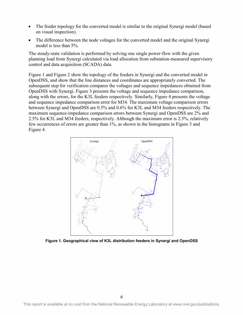
6 This report is available at no cost from the National Renewable Energy Laboratory at www.nrel.gov/publications.
• The feeder topology for the converted model is similar to the original Synergi model (based on visual inspection).
• The difference between the node voltages for the converted model and the original Synergi model is less than 5%.
The steady-state validation is performed by solving one single power-flow with the given planning load from Synergi calculated via load allocation from substation-measured supervisory control and data acquisition (SCADA) data.
Figure 1 and Figure 2 show the topology of the feeders in Synergi and the converted model in OpenDSS, and show that the line distances and coordinates are appropriately converted. The subsequent step for verification compares the voltages and sequence impedances obtained from OpenDSS with Synergi. Figure 3 presents the voltage and sequence impedance comparison, along with the errors, for the K3L feeders respectively. Similarly, Figure 4 presents the voltage and sequence impedance comparison error for M34. The maximum voltage comparison errors between Synergi and OpenDSS are 0.5% and 0.6% for K3L and M34 feeders respectively. The maximum sequence-impedance comparison errors between Synergi and OpenDSS are 2% and 2.5% for K3L and M34 feeders, respectively. Although the maximum error is 2.5%, relatively few occurrences of errors are greater than 1%, as shown in the histograms in Figure 3 and Figure 4.
Figure 1. Geographical view of K3L distribution feeders in Synergi and OpenDSS

7 This report is available at no cost from the National Renewable Energy Laboratory at www.nrel.gov/publications.
Figure 2. Geographical view of M34 distribution feeders in Synergi and OpenDSS
Figure 3. Percentage error of voltage (left) and sequence impedance (right) with respect to
distance from the feeder head for K3L feeders

8 This report is available at no cost from the National Renewable Energy Laboratory at www.nrel.gov/publications.
Figure 4. Percentage error of voltage (left) and sequence impedance (right) with respect to
distance from the feeder head for M34 feeders
2.2 Design of Secondary Circuits Recently, utility companies across the United States put considerable effort toward improving the way they represent distribution systems, and—like the Companies—have sizeable portions of their distribution feeders represented in a distribution software tool such as Synergi, CYMDIST, or DEW. To the best knowledge of the authors, however, there is no utility that has accurate or realistic representations or models of the low-voltage secondary networks. In this project, it is critical to add the necessary level of detail to more accurately capture not only the annual voltages at the primary medium-voltage level, but also at the secondary low-voltage level to which PV systems are connected and which are required to meet tariff requirements.
To add more-accurate representations of secondary circuits, the aggregate load nodes (or service transformer nodes) in feeder M34 and feeder L are classified into customer types to design secondary circuits based on this customer classification, and then automate the building of such circuits in the OpenDSS model. The goal is to add more detail to the medium-voltage distribution models—including service transformers and secondary circuits in the OpenDSS model as shown in Figure 5—to capture the voltage drop that occurs from the medium-voltage bus to the customer house where the PV system inverters are connected, and ultimately more accurately simulate the voltage at the terminals of the residential inverters. Most of the advance inverter modes to be studied in this project are control functions that depend on the local voltage sensed by the inverter, and thus show the importance of capturing the voltage drops in secondary circuits.

9 This report is available at no cost from the National Renewable Energy Laboratory at www.nrel.gov/publications.
Figure 5. Diagram showing the load model provided by Hawaiian Electric on the left, and the
detailed load transformer and secondary circuit being added by NREL to the existing model for every load node
To classify load nodes into customer types, the internal NREL GIS department superimposed the coordinates of each load node on top of the land-use type to classify the load nodes into customer types. The maps for M34, and K3L are shown in Figure 6 and Figure 7 respectively.

10 This report is available at no cost from the National Renewable Energy Laboratory at www.nrel.gov/publications.
Figure 6. Customer load nodes overlaid on GIS land-use database for M3 and M4 loads
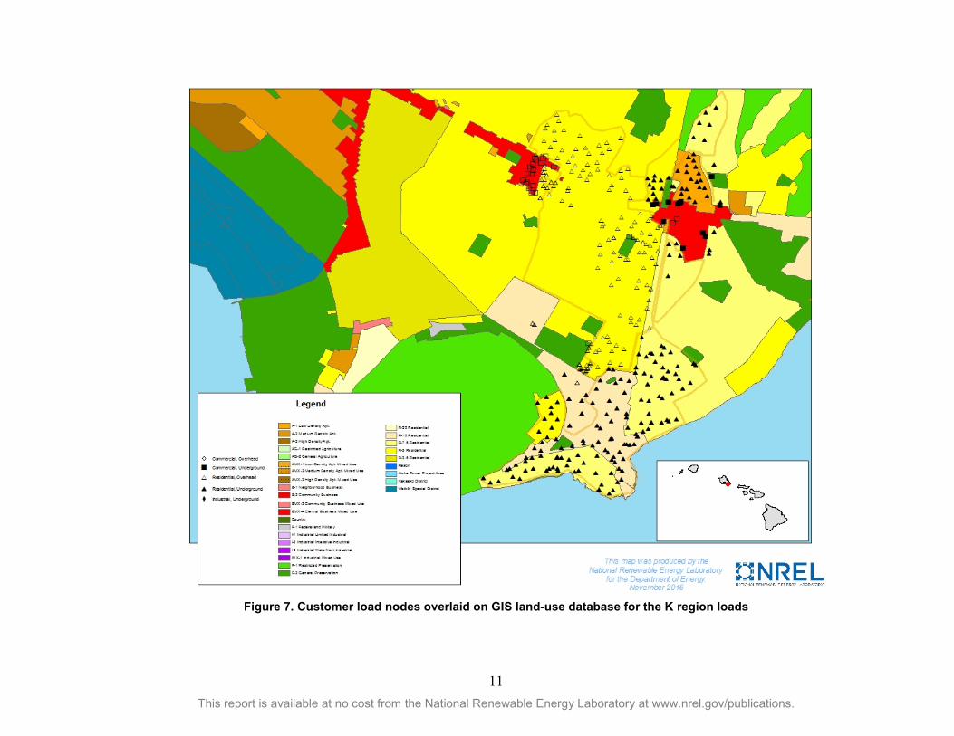
11 This report is available at no cost from the National Renewable Energy Laboratory at www.nrel.gov/publications.
Figure 7. Customer load nodes overlaid on GIS land-use database for the K region loads

12 This report is available at no cost from the National Renewable Energy Laboratory at www.nrel.gov/publications.
The customer types are selected based on the GIS classification and availability of secondary designs, as shown in Table 1. Hawaiian Electric provided 55 detailed designs to be used to add low-voltage circuits to the existing model. The Hawaiian Electric team was consulted to determine that the commercial and multifamily aggregated load nodes will be kept at the primary level in the model, because there is no significant voltage drop expected at those customer locations with typically oversized secondary circuits. For the overhead rural customers, NREL proposed the following secondary build-out assumptions: (1) customers are 200 ft. apart from each other, (2) overhead #2 cable size is used for secondary lines, and (3) there are 6 customers per shared secondary circuit.
Table 1. Secondary Circuit Designs for Each Customer Type
Customer Type Description of Secondary Designs (x Number of Designs)
M3 UG Residential Housing developer detailed drawings (x 30)
M4 UG Residential Housing developer detailed drawings (x 11)
Feeder L UG Residential Companies secondary upgrade designs (x 3)
OH Residential Companies secondary upgrade designs (x 11)
OH Rural NREL proposed design
Along with the customer type, each load node has the following information extracted from the Synergi model, as shown in Table 2 for an example load node “OH_1.”
Table 2. Load Classification to Map Each Aggregate Load Node Provided by Hawaiian Electric to a Secondary Design
Load Node Cust. Type Xfmr Size [kVA] # Cust. P [kW] Existing PVs
OH_1 OH Residential 50 10 13 PV1, PV2
After the load nodes are classified into customer types with a pool of secondary designs associated, the methodology proposed to build the secondary circuits for underground (UG) and overhead (OH) residential customer types is shown in the flowchart diagram in Figure 8.The process shown in Figure 8 is automated in Python to create the OpenDSS files of all secondary transformers, lines, and each load representing a house and a customer PV system.

13 This report is available at no cost from the National Renewable Energy Laboratory at www.nrel.gov/publications.
Figure 8. Flowchart showing the methodology to assign a secondary design process to
OH and UG residential customers from a total of 55 detailed secondary designs provided by Hawaiian Electric
2.3 Data Processing for Time Series A significant effort in this project is to synthesize the data that will drive the time-series model. As it often is said, “the model of distribution feeders is only as good as the data you feed into it,” and, as such, this step is critical in this project to create load data and solar data that represents as best as possible what occurs in the real world.
This section describes the process and results to back-out what is referred to as “gross load”—which is the load in the feeder without solar PV systems—and to create a power PV production profile. The individual feeder gross load then is used to drive the load time series, and the PV profile is used to drive the PV systems in the model.
The data obtained from Hawaiian Electric for this process is:
• Substation yearly SCADA voltage, current, and real and reactive power for 2015
• Individual feeder yearly SCADA voltage, current, and real and reactive power as available for 2015

14 This report is available at no cost from the National Renewable Energy Laboratory at www.nrel.gov/publications.
• Megawatt-hours/megawatt hourly PV power production for two PV regions of interest on O‘ahu
• Irradiance 15-minute profiles for the two PV regions of interest on O‘ahu
• AMI customer meter 15-minute kilowatt-hour and voltage.
2.3.1 Replacing Missing and Outlier Data This section describes how the missing and outlier for 2015 feeder substation real and reactive power data is replaced. The first step in the data-processing task is to identify the missing and outlier data and replace it. An example of outlier data occurs where the outlier data corresponded to reconfiguration events in which a feeder picked up loads from a circuit in another substation, which is shown by abnormally high loading. Due to the very good correlation of circuits within a substation, circuit data due to load-transfer events was replaced with the adjacent circuit data connected to the same substation. For missing data (when there were overall SCADA outages) the data was replaced with the most appropriate adjacent (in time and day of week) time series data.
This process is illustrated in Figure 10 for the M3 feeder. The M3 and M4 feeder real and reactive power correlation is shown in the bottom-left regression plot in Figure 9, and M3 is replaced with M4 circuit data and vice versa during load-transfer events. The M3 raw SCADA circuit real power data is shown in blue and the replaced data from M4 is highlighted in red.
Figure 9. Linear Regression between M3 and M4 circuit load.

15 This report is available at no cost from the National Renewable Energy Laboratory at www.nrel.gov/publications.
Figure 10. M3 outlier data-replacement example with M4 data

16 This report is available at no cost from the National Renewable Energy Laboratory at www.nrel.gov/publications.
2.3.2 Estimating Gross Load in the Feeders The following section describes how to estimate the gross load (also sometimes referred to as “native” load)—that is, the load profile as if there was no PV system installed in the feeders. During nighttime hours, the gross load and the measured SCADA data net load are the same. During daytime hours, however, the objective is to determine the shape of the demand without solar production. The process first is described for M34 circuits and then for K3L feeders.
2.3.2.1 Backing Out Gross Load for M34 Feeders For the M34 substation circuits, the real and reactive power regression method (PQ regression method) was used to estimate what the load on each circuit is without any solar PV systems. Due to the fairly invariable power factor in M3 and M4 feeders during nighttime hours (as shown in Figure 11), and because predominantly residential customers are served, the reactive power can be used to determine the real power during daytime hours. This assumption only works if the existing solar PV systems are connected at unity power factor, which is the case in M3 and M4 circuits.
Figure 11. Nightime M3 and M4 power factors for 2015
In M4 feeder, the reactive power during the day was not as constant as M3 due to larger commercial loads; however, the reactive power of M3 was used as a proxy to the reactive power in M4. The real versus reactive power regression curves are shown in Figure 12.

17 This report is available at no cost from the National Renewable Energy Laboratory at www.nrel.gov/publications.
Figure 12. Nighttime real versus reactive power regression for M34 circuits using M3 reactive
power data for both
The advantages of using the PQ regression method are that it relies on power measurements, and it is independent of estimating how much PV energy is in the system and its profile. The other method explored for backing-out gross load is to estimate the PV production for each of the feeders and subtract that from SCADA net load at each time step. For this, Hawaiian Electric provided MWh/MW values versus irradiance of a fleet of systems in the M34 region. The MWh/MW values essentially are a PV fleet real-power production metric that takes into account PV systems’ orientation and losses.
Figure 13 shows the morning values highlighted in red and the afternoon values in blue. These are shown along with the degree 3 polynomial fit of the distribution of all of the values. The polynomial MWh/MW curve multiplied by the megawatts of total installed PV systems for each circuit gives an estimate of the PV production at every given time step. Note that the MWh/MW curve was provided hourly, and the SCADA net load is processed at 15-minute time steps. Because Hawaiian Electric also provided typical 15-minute plane of array (POA) irradiance curve for the M34a region, NREL estimated a final MWh/MW 15-minute curve using the irradiance profile.
The results of the PQ regression method and MWh/MW method are shown in Figure 14 for M3 and Figure 15 for M4 for September 14–18, 2015, using total installed PV systems in 2015 (the sum of executed residential projects and feed-in-tariff projects). The figures also include the SCADA real and reactive net power and the estimated aggregate PV profiles from both methodologies. Note that, for M4, the estimated gross load for the MWh/MW method produces a load shape with deep valleys during the day, and the load in the middle of the day is nearly as low as the minimum nighttime load that typically occurs around 3 a.m. This load profile is very unlikely even with mainly residential customers being served by the circuits. The estimated aggregate PV profile from the PQ regression method comes from subtracting the SCADA net power measured from the estimated gross load.

18 This report is available at no cost from the National Renewable Energy Laboratory at www.nrel.gov/publications.
Figure 13. The MWh/MW values versus irradiance for a fleet of PV systems in the M34 region
Figure 14. The M3 real power and PV system production estimates produced using the
PQ regression method versus the MWh/MW method

19 This report is available at no cost from the National Renewable Energy Laboratory at www.nrel.gov/publications.
Figure 15. The M4 real power and PV-production estimates using the PQ regression method
versus the MWh/MW method
The two gross load estimates were compared to 2008 SCADA substation data, as shown in Figure 16, and it is determined that the PQ regression method provides a closer estimate of what the power would look like if there was no PV energy in the system, because in 2008 there were almost no residential PV systems installed in the M34 circuits. The 2008 net load substation data does not correspond exactly to September 14–18 because the 2008 data was shifted to match the same day of the week in the same week in September.
2.3.2.2 Backing out Gross Load for K3L Feeders The PQ regression method could not be used due to large inductive loads during daytime hours on both K3L feeders, making the PQ regression method invalid because it is based on nighttime real and reactive power correlation. Thus, K3L circuits required the use of the MWh/MW method. Figure 17 shows what the gross load profile would look like for the K3L substation for September 14–17, 2015, using the PQ regression method (shown in orange), and the gross load using the MWh/MW regression method (shown in red). Those can be compared to the measured net load in 2012 (shown in purple) when there was significantly less penetration of solar in the circuits.

20 This report is available at no cost from the National Renewable Energy Laboratory at www.nrel.gov/publications.
Figure 16. M34 Substation gross real power estimates from MWh/MW and PQ regression methods
compared to 2015 and 2008 substation net load profiles (top—real power; bottom—scaled and normalized)
Figure 17. The K3L substation gross real power estimates from MWh/MW and PQ regression
methods compared to 2015 and 2012 substation net load profiles
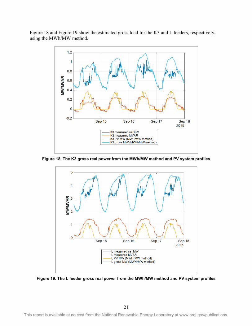
21 This report is available at no cost from the National Renewable Energy Laboratory at www.nrel.gov/publications.
Figure 18 and Figure 19 show the estimated gross load for the K3 and L feeders, respectively, using the MWh/MW method.
Figure 18. The K3 gross real power from the MWh/MW method and PV system profiles
Figure 19. The L feeder gross real power from the MWh/MW method and PV system profiles

22 This report is available at no cost from the National Renewable Energy Laboratory at www.nrel.gov/publications.
2.3.2.3 Summary of Gross Load and PV Profile Generation For the M34 feeders, the MWhr/MW method using any of the values provided by Hawaiian Electric for total installed megawatts of solar PV in 2015 doesn’t result in a monotonically increasing load profile similar to 2008 historical data. The PQ regression method results in a gross load profile similar to that for 2008.The PQ regression method is not based on any assumption of PV in the feeders and uses just the real and reactive power correlation at night from measured SCADA substation data; thus, it can be used to estimate the amount of solar energy in the feeders. The data-processing effort performed in M34 feeders is summarized in the flowchart in Figure 20. The goal is to create a load shape and a PV shape to be used in the OpenDSS modeling effort to drive the time-series simulation with different amounts of PV penetration.
In the K3L feeders, the PQ regression method was not a viable approach due to reactive power step changes during daytime business hours. This effectively makes the PQ regression not applicable because it is generated based on nighttime data and assumes a similar gross load power factor during daytime. The MWh/MW method is the only tenable solution for these feeders; however, its disadvantage is that it relies on the assumption of total installed PV systems in 2015 in the circuits. In each case, the value of total installed PV systems was chosen based on the value that provides the load profile closer to the historical substation data provided when there was significantly less PV in the system. The flowchart summarizing the data processing methodology used for the K3L feeders is shown in Figure 21.
Figure 20. Flowchart summarizing the data processing of load and PV energy for M34 feeders
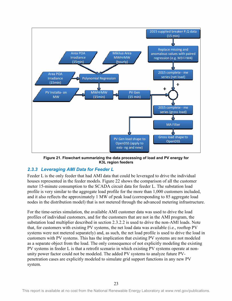
23 This report is available at no cost from the National Renewable Energy Laboratory at www.nrel.gov/publications.
Figure 21. Flowchart summarizing the data processing of load and PV energy for
K3L region feeders
2.3.3 Leveraging AMI Data for Feeder L Feeder L is the only feeder that had AMI data that could be leveraged to drive the individual houses represented in the feeder models. Figure 22 shows the comparison of all the customer meter 15-minute consumption to the SCADA circuit data for feeder L. The substation load profile is very similar to the aggregate load profile for the more than 1,000 customers included, and it also reflects the approximately 1 MW of peak load (corresponding to 85 aggregate load nodes in the distribution model) that is not metered through the advanced metering infrastructure.
For the time-series simulation, the available AMI customer data was used to drive the load profiles of individual customers, and for the customers that are not in the AMI program, the substation load multiplier described in section 2.3.2.2 is used to drive the non-AMI loads. Note that, for customers with existing PV systems, the net load data was available (i.e., rooftop PV systems were not metered separately) and, as such, the net load profile is used to drive the load in customers with PV systems. This has the implication that existing PV systems are not modeled as a separate object from the load. The only consequence of not explicitly modeling the existing PV systems in feeder L is that a retrofit scenario in which existing PV systems operate at non-unity power factor could not be modeled. The added PV systems to analyze future PV-penetration cases are explicitly modeled to simulate grid support functions in any new PV system.

24 This report is available at no cost from the National Renewable Energy Laboratory at www.nrel.gov/publications.
Figure 22. Feeder L circuit 15-min SCADA data compared to the aggregate AMI customer meters; the comparison reflects that there is approximately 1 MW of demand that is not metered via AMI
(the x-axis represents time in 15-min interval for a year).
2.4 Time Series Model Validation The previously described OpenDSS models were validated in a steady state, and as such were run at one single instance of time, assuming that the loads are all fixed at planning load and the PV systems are producing rated power. This section takes the multipliers derived from the data-processing section for (1) gross load to drive the load profiles in the model, and (2) PV systems to drive the PV profiles.
The load and PV multipliers for September 14–17, 2015, are used to validate the time series model with Grid 20/20 measurement data provided by Hawaiian Electric located at the secondary terminals of distribution service transformers on the feeders. This period was selected for time-series validation due to the availability of Grid 20/20 data for most of the transformers provided and relatively clear-sky day PV profiles.
2.4.1 Time Series Validation with Grid 2020 Data for M34 The results of driving the OpenDSS timeseries model with the multipliers are described below. Note that, for the M34 feeders, only September 16–17, 2015, data were used for validation because the Grid 20/20 field measurements were missing several hours of data from September 14–15.

25 This report is available at no cost from the National Renewable Energy Laboratory at www.nrel.gov/publications.
Figure 23 and Figure 24 show the real power and voltage at the eight Grid 20/20 measurement locations in M34 feeders. For the most part, the real power matches remarkably well with the measured load at the secondary transformer locations, in particular when there is PV energy at customers’ systems connected at that point. In some locations, the real power is significantly greater or lesser than the simulation aggregate load at those locations, which is expected when comparing field load data with estimated model data. The same applies to the higher-frequency noise profile of the field data, as compared to the smoother gross load profile. As mentioned, however, the variability of PV energy is fairly well represented from the PV profile estimated in the data-processing effort described above.
When comparing voltages at the measurement locations, the voltage profile of the OpenDSS model matches the field data. Note that the other very important operating variable that can be validated is that the LTC in the model is behaving very much like in the field, as the step changes and voltage profiles driven by the LTC regulation in both field and modeled voltages can be seen.
2.4.2 Time Series Validation with AMI Data for Feeder L For feeder L, the maximum and minimum voltage envelope for aggregate measured voltages for all metered customers compared to the aggregate envelope of simulated voltages is shown in Figure 25 for the highest-voltage week of 2015 (May 20 through May 27). Note that there are 85 aggregate loads in the top graph that are driven by the substation multiplier. A subset of those aggregates is located close to the substation and is driving the maximum envelope profile during non-PV system production hours; that is not reflected in the AMI aggregate voltage profile.
Figure 26 and Figure 27 show the same voltage envelope comparison plots between simulated and measured data for three specific service transformer locations. The exact representation of secondary distribution circuits in the model and exact locations of the AMI meters were not available (but rather only which service transformer the AMI meters are connected to), so the comparison is of the envelope of maximum and minimum simulated and measured customer voltage data connected to the same transformer. The maximum and minimum demonstrate how well estimated the voltage is at the beginning and at the end (respectively) of a secondary circuit.
Figure 26 is representative of a secondary circuit in which the simulated voltage envelope matches the measured voltage fairly well in terms of both amplitude and overall profiles. In Figure 27 the top graph is representative of a secondary circuit in which the model underestimates the voltage magnitude but still provides a good approximation of the time-series voltage profiles; the bottom graph is representative of a secondary circuit in which the model overestimates the voltage magnitude. As such, in the simulated model for feeder L, the voltages might not precisely match the voltages measured at the customer meter locations, but the overall range of simulated voltages and measured voltages are well approximated.
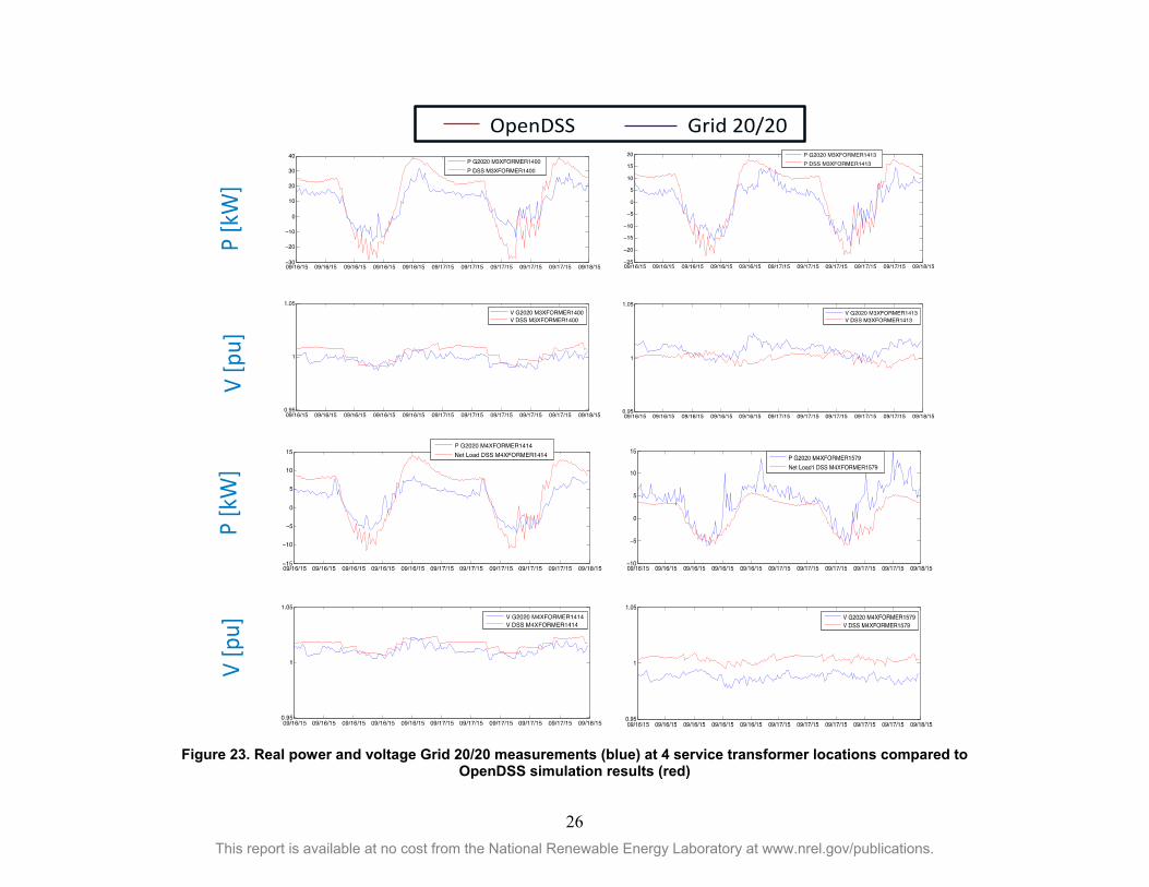
26
This report is available at no cost from the National Renewable Energy Laboratory at www.nrel.gov/publications.
Figure 23. Real power and voltage Grid 20/20 measurements (blue) at 4 service transformer locations compared to
OpenDSS simulation results (red)
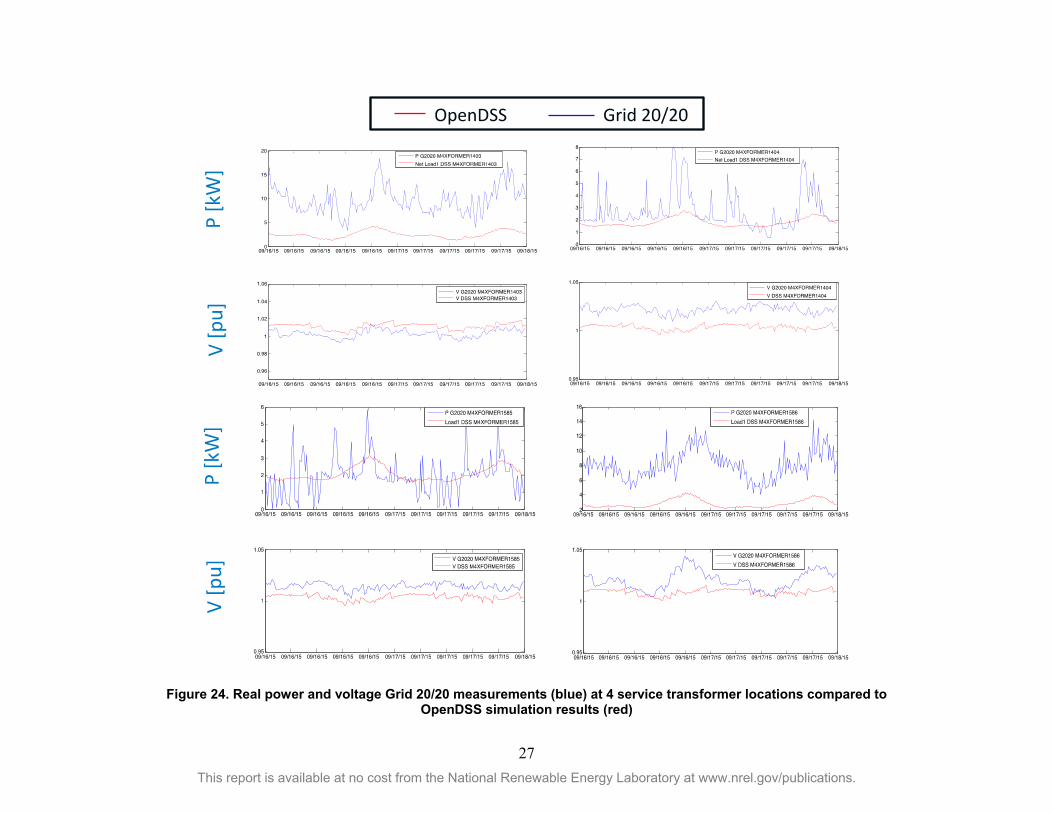
27
This report is available at no cost from the National Renewable Energy Laboratory at www.nrel.gov/publications.
Figure 24. Real power and voltage Grid 20/20 measurements (blue) at 4 service transformer locations compared to OpenDSS simulation results (red)

28 This report is available at no cost from the National Renewable Energy Laboratory at www.nrel.gov/publications.
Figure 25. Envelope of maximum and minimum voltages for simulated load (top) and measured AMI loads (bottom) for all customer
loads in feeder L.

29 This report is available at no cost from the National Renewable Energy Laboratory at www.nrel.gov/publications.
Figure 26. Envelope of maximum and minimum voltage across the secondary circuit of a service transformer location in which
maximum and minimum simulated (top) and measured (bottom) voltage envelopes match well.

30 This report is available at no cost from the National Renewable Energy Laboratory at www.nrel.gov/publications.
Figure 27. Envelope of maximum and minimum voltage across the secondary circuit of two service transformer locations (top: underestimation, bottom: overestimation).

31 This report is available at no cost from the National Renewable Energy Laboratory at www.nrel.gov/publications.
2.4.3 Preliminary Evaluation of Current LTC Operations The voltage profiles at the secondary transformer locations suggest that the load tap changers in the OpenDSS feeder models are performing a control strategy similar to that of one implemented in the field. The LTC settings are revised in subsequent sections when PV energy is added to the current 2015 baseline feeder models and legacy LTC settings are inadequate to deal with reverse power flow at the substation.
2.5 Final 2015 Baseline Feeder Models Two 12.47-kV substations are included in the remainder of the study: (1) Substation M with both feeders—M3 and M4—fully modeled, and (2) Substation K with only feeder L modeled in full detail and feeder K3 aggregated at the substation. The characteristics of both 12.47-kV M34 and L feeders are included in Table 3.
Feeder M34 was selected specifically because of the diversity of the different types of PV installations already existing on a circuit—residential, commercial, and large feed-in-tariff (FIT) projects that are approximately 500 kW each. Analyzing this circuit provided an understanding of the impacts of advanced inverter functions with and without larger projects. Due to the existing voltage issues with high amounts of unity power factor PV, the question of how effective GSF in the near and longer term future are on voltage performance for all customers is very relevant.
Feeder L was selected because of the difference in location and types of customers in comparison to Feeder M34. Feeder L is located in a high-density residential area, and it was suspected that this variable would have a great impact on the effectiveness of the advanced inverter functions. Feeder L also has AMI data that was used to understand the modeling aspect of load diversity.
Table 3. M34 and L General Feeder Characteristics

32 This report is available at no cost from the National Renewable Energy Laboratory at www.nrel.gov/publications.
The 2015 baseline primary voltage heat-map for M34 feeders for June 9—which is the day that had the highest voltage of the year—is shown in Figure 28. At 11:15 a.m., when solar PV systems produce at maximum power, the substation LTC reduces the primary voltage to accommodate for voltage increase at the secondary voltage level, but at the same time does not create undervoltages. In the evening, at 7:30 p.m., when there is no solar PV energy produced, the substation LTC is operated at the higher end of the allowable voltage range with the use of line drop compensation (LDC). Figure 29 shows the voltage to distance from the substation plot for both M3 and M4 feeders; primary voltages are relatively flat, and the bulk of the voltage drop or rise occurs in the service transformer and secondary circuits. This demonstrates the importance of the effort to approximate secondary circuits as accurately as possible.
Feeder L 2015 baseline primary voltages heat-map has a voltage-management strategy during daytime loading similar to that of M34. During the evening, however, because the legacy LTC voltage control is greater than normal (121 V versus 120 V), and the reactance in the line drop compensations is 0, the primary voltage is similar to that during daytime conditions in the areas near the substation (see Figure 30). Very much like M34 feeders, primary voltages in feeder L are very flat and most of the voltage drop occurs in the secondary circuits, as shown in Figure 31.
Figure 28. June 9, 2015, highest (left) and lowest (right) voltage heat map for M3 and M4 feeders

33 This report is available at no cost from the National Renewable Energy Laboratory at www.nrel.gov/publications.
Figure 29. Voltage to distance from the substation plot of primary voltages (solid lines) and
secondary voltages (dotted lines) for M3 and M4 feeders on June 9 at 11:15 a.m.
Figure 30. May 23, 2015, highest (left) and lowest (right) voltage heat map for feeder L

34 This report is available at no cost from the National Renewable Energy Laboratory at www.nrel.gov/publications.
Figure 31. Voltage to distance from the substation plot of primary voltages (solid lines) and
secondary voltages (dotted lines) for feeder L on May 23 at 12:30 p.m.
In the 2015 baseline feeder models described above, additional PV energy is added to simulate near-term and long-term future scenarios, and to show how activating advanced inverter features in any new rooftop PV system that is interconnected impacts the voltage-management strategies for the feeders.
3 Time-Series Simulation and Modeling of Advanced Inverter Modes
This section describes the methodology used to perform annual quasi-static time-series simulations as well as the advanced inverter functions that are modeled.
3.1 PV Systems—Assumptions and Advanced Inverter Modes The PV systems were modeled using the OpenDSS “PVSystem” object [12]. The main assumptions on the PV systems are described below.
• PV panel to inverter capacity in ratio is 1.2.
• Used a 0.1 % capacity rating of inverter to turn on or off. When the inverter is off or on, the power from the array must be greater than or less than 0.1 % for the inverter to turn on or off, respectively.
• Inverters do not turn off with overvoltages or undervoltages. In reality, inverters disconnect when voltages remain greater than 1.1 pu or less than 0.88 pu for some time to comply with the requirements of IEEE 1547-2003 and other interconnection

35 This report is available at no cost from the National Renewable Energy Laboratory at www.nrel.gov/publications.
standards. The approach taken in this study, however, is to leave them turned on to better evaluate the effectiveness of a given voltage-management strategy in not creating voltages greater than 1.1 pu. If PV systems were to turn off at 1.1 pu, then voltages in the system would decrease, but it would be harder to determine whether the effectiveness of the advanced inverter mode under evaluation was due to PV systems turning off and as a result lowers voltages, or if it instead is due to the inverter grid support function itself. From the utility’s perspective, the interest is in seeing how high voltages would be to evaluate how to reduce voltages so that there aren’t any PV systems that turn off due to such high voltages.
This assumption implies that the simulated voltages in the very high PV penetration cases presented in section 4 are higher than they would be expected to occur in the field. However, due to voltages being higher (versus lower) with this assumption, the impact to the metrics calculated in this VROS project and described in section 4.1 (DeltaV, annual energy curtailment, etc.) is that such metrics would be lower. In the energy curtailment calculations to PV customers with GSF activated, energy reduction from PV systems that would have been turned off due to the 1.1 pu voltage disconnection requirement in IEEE 1547-2003 was not included. This avoids attributing the energy curtailment to PV customers that would have been disconnected in reality due to the disconnection requirement in the interconnection standard to the energy reduced from activating a certain GSF.
For each PV penetration case described in the following section, the PV systems with advanced inverter (AI) functionalities is run in the following advanced inverter modes:
• CPF 0.95
• Volt-VAR
• CPF 0.95 in combination with volt-watt
• Volt-VAR in combination with volt-watt. All the modes given above are modeled with reactive power priority, which is how Hawaiian Electric Companies have chosen to implement grid support functions and, as such, PV kilowatt-hour reduction at the customer site can occur in all modes. The settings for the modes listed above are shown in Figure 32. A power factor of 0.95 absorbing VARs (negative convention in Figure 32) with current leading voltage is chosen for CPF mode as defined in Hawai‘i Rule 14H, which corresponds to 33% of the maximum rated voltages at full kVA output. The volt-VAR curve corresponds to a moderate curve with a deadband of ± 0.03 pu, and a droop curve above 1.03 and below 0.93 pu. The droop slope reaches full VAR absorption at 1.06 pu and full VAR generation at 0.94 pu. Full VARs are defined as 44% of the inverter apparent power rating which corresponds to power factor of 0.9 at full apparent power. Thus volt-VAR can absorb (or produce) more reactive power than a constant power factor of 0.95. The full VAR capability, however, only is used when the voltage is far from nominal.
The volt-watt function initiates reduction in real power when the voltage at the PCC (not necessarily the inverter terminals) crosses 1.06 pu. ANSI C84.1 Standard [13] provides that voltage delivered at the point of common coupling (PCC) generally should be provided at ±.05 pu, and so volt-watt provides means to protect utility voltages from greatly exceeding ANSI C84.1 service voltage ranges.

36 This report is available at no cost from the National Renewable Energy Laboratory at www.nrel.gov/publications.
Figure 32. Advanced inverter mode settings for constant power factor, volt-VAR, and volt-watt
3.2 Implementation of Inverter Controls in OpenDSS Several challenges arose in implementing the grid support functions in OpenDSS. Although OpenDSS natively supports some version of each grid support function mentioned above, at the time that this research was conducted it did not support the exact versions and combinations of each function desired for this study. Hence, Python scripts were written to interact with OpenDSS to implement the desired functions. The challenges faced and the solutions found are described below.
Only the volt-VAR function was implemented using the native inverter control object in OpenDSS. It was implemented with the settings previously described and reactive power priority. The constant power factor and volt-watt were programmed in Python (not using OpenDSS), however, and the real and reactive power values were updated directly in the PVSystem object in OpenDSS.
OpenDSS makes the constant power factor an accessible value of the PVSystem object that can be changed. However, OpenDSS did not have a variable for implementing constant power factor with reactive power priority (instead the only implementation of CPF is with watt priority). To overcome this, the real and reactive power calculations are performed in Python and then are updated in the PVSystem object in OpenDSS as follows.
1. Calculate reactive power q based using equation (1), with pbefore being the real power from the PV profile and pf the power factor value of 0.95.
𝑞𝑞 = 𝑝𝑝𝑏𝑏𝑏𝑏𝑏𝑏𝑏𝑏𝑏𝑏𝑏𝑏 ∗ tan (acos(𝑝𝑝𝑝𝑝)) (1)
37 This report is available at no cost from the National Renewable Energy Laboratory at www.nrel.gov/publications.
2. Determine whether q is greater than 44% of kVA capacity, and if so, set q to 44% of kVA capacity.
3. Determine whether �𝑝𝑝𝑏𝑏𝑏𝑏𝑏𝑏𝑏𝑏𝑏𝑏𝑏𝑏2 + 𝑞𝑞2 > 𝑘𝑘𝑘𝑘𝑘𝑘 (kVA being the rated capacity of the inverter) and if it is, then calculate pcurtailed based on q and kVA with pcurtailed being the actual inverter power after curtailment. 4. Update the PVSystem object with q and pcurtailed using “kvar” and “pctPmpp” OpenDSS variables (only if the result of step 3 is positive).
For volt-watt, although OpenDSS has a volt-watt “inverter control” object mode, the inverter control object could not be leveraged in combination mode with CPF. Following the calculation of CPF as explained above, if the OpenDSS “InvControl” object was used in volt-watt mode, and if the real power had been updated to pcurtailed via the pctPmpp variable, then the volt-watt InvControl would not incorporate that update, and it then increases the real power back to the original input pbefore value if the voltage did not exceed 1.06. In summary, the “inverter control” object in OpenDSS did not incorporate the update to the pctPmpp value of the PVSystem object. As such, the volt-watt algorithm was performed externally in Python following the CPF calculation described above.
The same issue occurred when performing volt-VAR and volt-watt one after the other. If volt-VAR with reactive power priority curtails real power, then performing volt-watt afterward brought the real power up to the pre-curtailed value if the voltage was less than or equal to 1.06 pu. OpenDSS recently began supporting the combination of volt-VAR with volt-watt via a new setting in the inverter control object called “CombiMode.” The latest release of OpenDSS (version 7.6.5.37), however, contained an error with volt-VAR in the combination mode. A Beta version of the software was posted in March 2017 on the sourceforge.net discussion board, but this version did not work for the feeder models in this study within the order of several hundred to a thousand PVSystem objects. As a result, it was decided that the best approach was to use the OpenDSS inverter control object for volt-VAR, and then perform the volt-watt algorithm externally in Python.
In both CPF 0.95 combined with volt-watt, and volt-VAR with volt-watt, the same volt-watt algorithm is programed in Python as described below. The variable dampfactor is included to assist with OpenDSS solver convergence with very large numbers of PV systems.
1. If the voltage at the PV system location is between 1.06 pu and 1.1 pu, then linear interpolation is performed to calculate the quantity of power to be curtailed pinterpolation. The new pcurtailed is calculated in equation (2), and the pctPmpp variable of the PV system is changed.
𝑝𝑝𝑐𝑐𝑐𝑐𝑏𝑏𝑐𝑐𝑐𝑐𝑐𝑐𝑐𝑐𝑏𝑏𝑐𝑐 = 𝑝𝑝𝑏𝑏𝑏𝑏𝑏𝑏𝑏𝑏𝑏𝑏𝑏𝑏 − 𝑑𝑑𝑑𝑑𝑑𝑑𝑝𝑝𝑏𝑏𝑐𝑐𝑐𝑐𝑐𝑐𝑏𝑏𝑏𝑏 ∗ �𝑝𝑝𝑐𝑐𝑖𝑖𝑐𝑐𝑏𝑏𝑏𝑏𝑖𝑖𝑏𝑏𝑐𝑐𝑐𝑐𝑐𝑐𝑐𝑐𝑏𝑏𝑖𝑖 − 𝑝𝑝𝑏𝑏𝑏𝑏𝑏𝑏𝑏𝑏𝑏𝑏𝑏𝑏� (2)
2. If the voltage exceeds 1.1 pu, then pcurtailed is set to 0. The value for the dampfactor in equation (2) is derived empirically by running the volt-watt algorithm in OpenDSS alone (not in combination mode) and then using the interpolation algorithm described above to generate the closest solution to the OpenDSS algorithm. The OpenDSS volt-watt algorithm goes through a number of iterations of interpolation to refine the least amount of curtailment that results in sufficient voltage support. To iterate through the COM

38 This report is available at no cost from the National Renewable Energy Laboratory at www.nrel.gov/publications.
interface in this project was time prohibitive, however, and the damping factor was found to be a good method to approximate empirically the iterative process in the volt-watt algorithm.
3.3 Time-Series Simulation with Advanced Inverters The program used to run OpenDSS through the COM interface is the Python programming language. A function called “main.py” is run via command line and the Python package “Click” is used to create command-line interfaces that define the following.
• feeder_name, help=name of the feeder
• input_dir, help=path to the OpenDSS master file
• masterfile, help=name of the master file
• sim_duration, help=simulation duration (daily, weekly, yearly)
• day_number, help=choose the start day for daily and weekly simulations
• day_duration, help=dayDuration
• time_steps_per_day, help=time steps in a day
• week_duration, help=weekDuration
• total_duration, help=yearlyDuration
• export_mode, help=light: loads, PV and regtaps; heavy: also includes node voltages
• smart_pv_mode, help=choose: none, volt-VAR, volt-VAR/volt-watt, CPF, CPF/volt-watt
• pf_value, default=1, help=for CPF choose the power factor value
• var_watt_priority, help=choose between VAR and watt
• casename, help=name of the output folder
• pvsystemlist, help=File with PV system names
• regulator_reverse_setting, help=Sets the LTC to legacy when no reverse power-flow or locks it when there is reverse power-flow
The high-level structure and logic of the Python code used to run the time-series simulation is described below.
1. Create a folder name casename_smart_pv_mode Create subfolders for all load voltages, all load powers, all PV powers, all PV reactive powers, all PV voltages, regulator taps, and feeder head real and reactive power
2. Assign the PV mode to PV systems in pvsystemlist only If smart_pv_mode is VV or VVW, then define volt-VAR curve and create inverter control object for all PV systems in pvsystemlist
39 This report is available at no cost from the National Renewable Energy Laboratory at www.nrel.gov/publications.
3. For day=day_number to day=day_number+total_duration/time_steps_per_day a. Create a “.csv” file for each subfolder created in step 1 (this creates a “.csv” file
per day) b. For time= time_steps_per_day*day_number to time=
time_steps_per_day*day_number+time_steps_per_day i. If smart_pv_mode is VV, then run power-flow
ii. If smart_pv_mode is CPF, then 1. run power-flow 2. perform the CPF algorithm as described, updating “kvar” property
for PV systems in pvsystemlist and “pctPmpp” property if necessary to curtail
3. run-power-flow again iii. If smart_pv_mode is CPFVW
1. run power-flow 2. perform the CPF algorithm as described, updating “kvar” property
for PV systems in pvsystemlist and “pctPmpp” property if necessary to curtail
3. run-power-flow again 4. create a sub-list of PV systems that are greater than 1.06 5. perform the volt-watt algorithm as described to update the
“pctPmpp” value of the PV systems in the bus-list from step iv 6. recalculate the reactive power corresponding to 0.95 power factor
based on the new real power output curtailed via the “kvar” PV system variable
7. run power-flow again iv. If smart_pv_mode is VVW
1. run power-flow 2. create a sub-list of PV systems that are greater than 1.06 3. perform the volt-watt algorithm as described to update the
“pctPmpp” value of the PV systems in the bus-list from step ii v. Extract all the data and append to the “.csv” files created in step 3.a.
Additional steps were added to the simplified algorithm described above to be able to change the legacy control settings of the LTC at high PV penetrations to lock it when there is reverse power-flow and prevent undervoltages.

40 This report is available at no cost from the National Renewable Energy Laboratory at www.nrel.gov/publications.
4 Results—Voltage Operating Strategies with Advanced Inverters
Weekly simulations at 15-minute time-steps are run for all the PV penetration cases and advanced inverter scenarios, and a subset of those are run annually. The week chosen for the simulation period is the highest-voltage week of the year from the 2015 load and PV system conditions.
4.1 Photovoltaic Penetration Cases and Metrics The PV penetration cases that are modeled with different advanced inverter functions are shown in Table 4 and Table 5 for M34 and L feeders respectively. For M34 feeders, a total of five cases were selected for scenario simulation.
• Case 0 Baseline o Case 0 corresponds to the 2015 baseline presented in a previous section with all
existing legacy rooftop and larger feed-in tariff systems interconnected at unity power factor; that is, not providing any reactive power support to regulate voltage.
o Case 0.AI, is a theoretical exercise to answer the question of how different the voltage profile the 2015 baseline case would be if all existing rooftop had advanced inverter features. As such, in Case 0.AI the 1.6-MW existing rooftop PV system is modeled with advanced inverter functions.
• Case 1 Baseline + Pending Projects o Case 1. PE-Rooftop, adds to Case 0 all the pending rooftop PV systems in the
Hawaiian Electric Companies’s tracking interconnection database with advanced inverter features. As such, this case represents the very near future of connecting all the rooftop PV systems in the interconnection queue with advanced inverter features.
o Case 1. PE-Rooftop+PE-FIT, adds also the larger FIT PV systems that are planned at unity power factor, as well as the pending rooftop PV systems.
• Case 2 Baseline + Pending Projects + Every Rooftop with PV o Case 2. High-Pen Rooftop, 2.3 MW of rooftop PV systems is added along with
the legacy 2015 rooftop and FIT PV, and the pending rooftop PV systems in Case 1. PE-Rooftop to achieve a total of 5.5 MW of rooftop solar PV. This case represents the very high PV penetration case, where every rooftop has a PV system (total of rooftop PV systems approximately equal to the peak load of the feeder).
o Case 2. High-Pen Rooftop+PE-FIT adds to the previous Case 2. High-Pen Rooftop the planned FIT PV systems.
The reason for creating different cases with and without larger planned FIT PV systems is to determine whether there is a difference in the effectiveness of advanced inverter functions activated in the smaller rooftop PV systems when there are larger PV systems connected at unity power factor. It also serves as another representative case as the typical residential distribution

41 This report is available at no cost from the National Renewable Energy Laboratory at www.nrel.gov/publications.
circuit does not have large quantities of FIT projects connected. In other words, the quantity (in megawatts) of advanced inverters stays the same in the two Case 1 and the two Case 2 instances; however, what changes is the total PV systems connected at unity power factor.
Table 4. M34 Feeders PV Penetration Cases
For feeder L, there are no existing or planned larger FIT systems and the PV penetration cases chosen for simulation with advanced inverters is simpler.
• Case 0 corresponds to the 2015 baseline presented in a previous section with all existing legacy rooftop PV systems interconnected at unity power factor, that is, not providing any reactive power support to regulate voltage.
• Case 1. PE-Rooftop adds to Case 0 all the pending rooftop PV systems in the Hawaiian Electric Companies’s tracking interconnection database with advanced inverter features. As such, this case represents the very near future of connecting all the rooftop PV systems in the interconnection queue with advanced inverter features.
• Case 2. High-Pen Rooftop, adds 2.7 MW of rooftop PV energy on top of the legacy 2015 rooftop and PV systems and the pending rooftop PV systems in Case 1. PE-Rooftop to achieve a total of 6.8 MW of rooftop PV energy. This case represents the very high PV-penetration case where every rooftop has a PV system (total of rooftop PV systems approximately equal to the peak load of the feeder).
Note that feeder L baseline 2015 case with all existing rooftop PV systems with advanced inverter functions is not modeled because 80% of the loads are driven by advanced metering infrastructure profiles and, for customers with existing PV systems, the net load profile with PV energy was used and PV systems were not explicitly modeled.

42 This report is available at no cost from the National Renewable Energy Laboratory at www.nrel.gov/publications.
Table 5. Feeder L PV Penetration Cases
For Case 2 PV penetration cases in M34 and L feeders, the methodology used to locate the additional rooftop PV to achieve a rooftop PV penetration of 100% with respect to peak load was to bias the location to service transformer locations that already served customers with rooftop PV. Each time a new PV system was added, it was also added to the list of PV systems used to bias the location of the next PV system added. With regard to the size of each rooftop PV, the methodology used the historical PV kW rating to customer peak load ratio of the existing rooftop PV in the feeder to size any new rooftop PV systems based on the size of the existing rooftop PV systems.
For each PV penetration case, the baseline of that case without advanced inverters is also run to compare the scenarios with advanced inverter features to it and derive comparative metrics to the PV penetration case without any voltage support from advanced inverters.
The voltage metric that is calculated for every advanced inverter scenario in a given PV-penetration case is DeltaV, and it is defined in equation 3 below.
𝐷𝐷𝐷𝐷𝐷𝐷𝐷𝐷𝑑𝑑𝑘𝑘 = 𝑉𝑉𝑚𝑚𝑚𝑚𝑚𝑚,𝐴𝐴𝐴𝐴−𝑉𝑉𝑚𝑚𝑚𝑚𝑚𝑚,𝐴𝐴𝐴𝐴𝑉𝑉𝑚𝑚𝑚𝑚𝑚𝑚,𝑚𝑚𝑛𝑛 𝐴𝐴𝐴𝐴−𝑉𝑉𝑚𝑚𝑚𝑚𝑚𝑚,𝑚𝑚𝑛𝑛 𝐴𝐴𝐴𝐴
(3)
Where Vmax,AI and Vmin,AI are the maximum and minimum customer voltages in the scenario with advanced inverter function, and Vmax,no AI and Vmin,no AI are the maximum and minimum customer voltages of the scenario without advanced inverter functions activated. As such, the lower the DeltaV metric, the more effective an advanced inverter function is in regulating voltage. The DeltaV metric is calculated between 10 a.m. and 2 p.m. to ensure that only voltage increase/decrease within maximum PV-system production hours is accounted for in the metric, and in particular to avoid including minimum voltages that might occur at night during non-PV-system generation hours.
The other metrics calculated for a given PV penetration case advanced inverter scenario with respect to the PV penetration without advanced inverters are related to impacts to the utility and the customer.
• Change in feeder head reactive power demand: This illustrates the increase in reactive power demand at the aggregate feeder head that could occur from PV advanced inverter functions absorbing reactive power locally.

43 This report is available at no cost from the National Renewable Energy Laboratory at www.nrel.gov/publications.
• Change in LTC number of operations: To quantify the impact of local voltage regulation at customer PV locations in legacy utility voltage-regulating equipment.
• Change in total number of customer voltage violations: To quantify the effectiveness of an advanced inverter function in reducing load voltage violations.
• Change in total kilowatt-hour energy production: For customer-owned PV systems to quantify the energy curtailment that can occur from activating grid support functions in customer-owned PV systems.
4.2 M34 Feeders Results The results of adding PV systems and activating advanced inverter functions in M34 feeders are described in this section. The voltage impacts are shown first and then the impacts to the utility and customers are presented.
4.2.1 Voltage Profiles and DeltaV Metric The voltage profiles for the highest-voltage week of the year, June 8 through June 15, for every customer meter modeled in the distribution model are shown and the DeltaV metric calculated.
4.2.1.1 Case 0 and Case 0.AI Voltages at every customer meter for Case 0, which represents the 2015 baseline conditions with existing legacy rooftop and FIT PV systems connected at unity power factor, show that there are existing overvoltage violations at a few customer meter locations due to the existing PV systems currently installed. As such, the feeder with the legacy utility voltage-regulation strategy already has a few customers that are operating outside the limit of the acceptable ANSI voltage range.
In the hypothetical case that all the existing rooftop PV systems currently in M34 feeders (which correspond to 47% of the total PV installed including existing FITs) would have been installed with 0.95 CPF or volt-VAR, the overvoltage violations could have been prevented, and both 0.95 CPF and volt-VAR have very similar effectiveness in regulating voltage during PV-system producing hours. This illustrates the benefit of activating advanced inverter voltage functionality as early as possible. Particularly on low-penetration circuits where there are opportunities to establish a “critical mass” of advanced inverters before voltage problems manifest themselves and where costly circuit upgrades are needed to mitigate voltage issues.
The results can be applied to future or developing circuits with growing amounts of PV projects. The results also can be used to understand whether all existing issues are mitigated and advanced inverters will be able to manage voltage rises on the secondary voltage level.

44 This report is available at no cost from the National Renewable Energy Laboratory at www.nrel.gov/publications.
Figure 33. Voltages at every customer meter in M34 feeders for the highest-voltage week of the year for Case 0
Figure 34. Voltages at every customer meter for M34 feeders for the highest-voltage week of the year for Case 0.AI
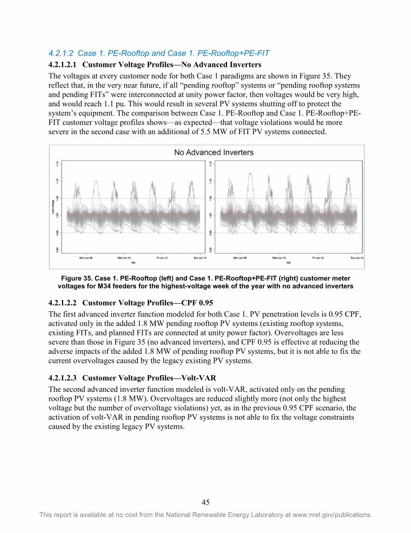
45 This report is available at no cost from the National Renewable Energy Laboratory at www.nrel.gov/publications.
4.2.1.2 Case 1. PE-Rooftop and Case 1. PE-Rooftop+PE-FIT 4.2.1.2.1 Customer Voltage Profiles—No Advanced Inverters The voltages at every customer node for both Case 1 paradigms are shown in Figure 35. They reflect that, in the very near future, if all “pending rooftop” systems or “pending rooftop systems and pending FITs” were interconnected at unity power factor, then voltages would be very high, and would reach 1.1 pu. This would result in several PV systems shutting off to protect the system’s equipment. The comparison between Case 1. PE-Rooftop and Case 1. PE-Rooftop+PE-FIT customer voltage profiles shows—as expected—that voltage violations would be more severe in the second case with an additional of 5.5 MW of FIT PV systems connected.
Figure 35. Case 1. PE-Rooftop (left) and Case 1. PE-Rooftop+PE-FIT (right) customer meter
voltages for M34 feeders for the highest-voltage week of the year with no advanced inverters
4.2.1.2.2 Customer Voltage Profiles—CPF 0.95 The first advanced inverter function modeled for both Case 1. PV penetration levels is 0.95 CPF, activated only in the added 1.8 MW pending rooftop PV systems (existing rooftop systems, existing FITs, and planned FITs are connected at unity power factor). Overvoltages are less severe than those in Figure 35 (no advanced inverters), and CPF 0.95 is effective at reducing the adverse impacts of the added 1.8 MW of pending rooftop PV systems, but it is not able to fix the current overvoltages caused by the legacy existing PV systems.
4.2.1.2.3 Customer Voltage Profiles—Volt-VAR The second advanced inverter function modeled is volt-VAR, activated only on the pending rooftop PV systems (1.8 MW). Overvoltages are reduced slightly more (not only the highest voltage but the number of overvoltage violations) yet, as in the previous 0.95 CPF scenario, the activation of volt-VAR in pending rooftop PV systems is not able to fix the voltage constraints caused by the existing legacy PV systems.
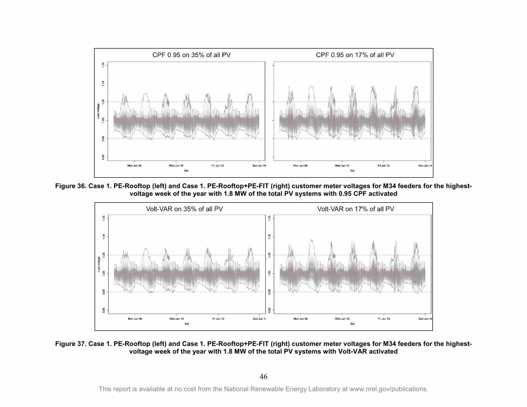
46 This report is available at no cost from the National Renewable Energy Laboratory at www.nrel.gov/publications.
Figure 36. Case 1. PE-Rooftop (left) and Case 1. PE-Rooftop+PE-FIT (right) customer meter voltages for M34 feeders for the highest-
voltage week of the year with 1.8 MW of the total PV systems with 0.95 CPF activated
Figure 37. Case 1. PE-Rooftop (left) and Case 1. PE-Rooftop+PE-FIT (right) customer meter voltages for M34 feeders for the highest-voltage week of the year with 1.8 MW of the total PV systems with Volt-VAR activated

47 This report is available at no cost from the National Renewable Energy Laboratory at www.nrel.gov/publications.
4.2.1.2.4 DeltaV for CPF 0.95 and Volt-VAR In both 0.95 CPF and volt-VAR scenarios, adding only the pending rooftop PV systems with advanced inverter features does not worsen the current 2015 voltage conditions. (Case 1. PE-Rooftop with 0.95 or volt-VAR has similar customer voltages to Case 0). If planned FITs are also interconnected at unity power factor as illustrated in Case 1. PE-Rooftop-PE-FIT, however, then other mitigation measures are required to prevent high voltages.
The effectiveness of 0.95 CPF and volt-VAR in regulating voltage is shown in the DeltaV metrics in Table 6. Due to being able to absorb slightly more reactive power in the volt-VAR curve (0.9 power factor) than 0.95 CPF, the DeltaV metric is slightly lower for volt-VAR than for CPF 0.95. Overall, however, the summary is that both advanced inverter functions are very similar in their effectiveness in regulating voltage.
Table 6. DeltaV (10 a.m. to 2 p.m.) for the Highest Voltage Week of the Year: Case 1. PE-Rooftop and Case 1. PE-Rooftop+PE-FIT with 0.95 CPF and Volt-VAR
PV Penetration Case PV Systems with
No GSF PV Systems
with GSF GSF
Evaluated DeltaV (10 a.m. to 2 p.m.) for a Week
Case 1. PE-Rooftop 1.6 MW
Existing Rooftop + 1.8 MW FITs
1.8 MW New Rooftop CPF -0.95 0.82
Case 1. PE-Rooftop 1.6 MW
Existing Rooftop + 1.8 MW FITs
1.8 MW |New Rooftop Volt-VAR 0.80
Case 1. PE-Rooftop +PE-FIT
1.6 MW Existing Rooftop
+ 7 MW FITs
1.8 MW New Rooftop CPF -0.95 0.81
Case 1. PE-Rooftop +PE-FIT
1.6 MW Existing Rooftop
+ 7 MW FITs
1.8 MW New Rooftop Volt-VAR 0.80
4.2.1.2.5 DeltaV for CPF 0.95/Volt-Watt and Volt-VAR/Volt-Watt The voltage profile plots for all customers for the highest-voltage week of the year for both Cases 1 are included in Appendix B. Customer voltage profiles look very similar to the CPF 0.95 and volt-VAR plots in Figure 36 and Figure 37 because there are not many PV-system customers that have system voltages greater than 1.06. The voltage effectiveness metric, as expected, is very similar to the scenario with just CPF 0.95 and volt-VAR (without volt-watt) as shown in Table 7.

48 This report is available at no cost from the National Renewable Energy Laboratory at www.nrel.gov/publications.
Table 7. DeltaV (10 a.m. to 2 p.m.) for the Highest Voltage Week of the Year: Case 1. PE-Rooftop and Case 1. PE-Rooftop+PE-FIT with 0.95 CPF/Volt-Watt and Volt-VAR/Volt-
Watt
PV Penetration Case PV Systems with
No GSF PV Systems
with GSF GSF
Evaluated DeltaV (10 a.m. to 2 p.m.) for a Week
Case 1. PE-Rooftop 1.6 MW Existing Rooftop + 1.8 MW FITs
1.8 MW New Rooftop
CPF -0.95 Volt-Watt
0.79
Case 1. PE-Rooftop 1.6 MW Existing Rooftop + 1.8 MW FITs
1.8 MW New Rooftop
Volt-VAR Volt-Watt
0.79
Case 1. PE-Rooftop +PE-FIT
1.6 MW Existing Rooftop
+ 7 MW FITs
1.8 MW New Rooftop
CPF -0.95 Volt-Watt
0.81
Case 1. PE-Rooftop +PE-FIT
1.6 MW Existing Rooftop
+ 7 MW FITs
1.8 MW New Rooftop
Volt-VAR Volt-Watt
0.80
4.2.1.3 Case 2. High-Pen Rooftop and Case 2. High-Pen Rooftop+PE-FIT 4.2.1.3.1 Customer Voltage Profiles—No Advanced Inverters In the very high PV-penetration Case 2 setups, with a rooftop PV penetration equal to the peak load of the feeder, the overvoltages are more than 1.15 pu, which in the field would imply that hundreds of PV systems are tripping offline due to the equipment overvoltage protections.
Figure 38. Case 2. High-Pen Rooftop (left) and Case 2. High-Pen Rooftop+PE-FIT (right) customer
meter voltages for M34 feeders for the highest-voltage week of the year with no advanced inverters
4.2.1.3.2 Customer Voltage Profiles—CPF 0.95 The customer voltages for Case 2. High-Pen Rooftop and Case 2. High-Pen Rooftop+PE-FIT show that activating 0.95 CPF in the pending 1.9 MW, and in any future rooftop system adding up to 5.5 MW, can mitigate the extreme overvoltages shown in Figure 38. This approach is not
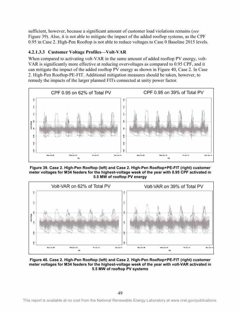
49 This report is available at no cost from the National Renewable Energy Laboratory at www.nrel.gov/publications.
sufficient, however, because a significant amount of customer load violations remains (see Figure 39). Also, it is not able to mitigate the impact of the added rooftop systems, as the CPF 0.95 in Case 2. High-Pen Rooftop is not able to reduce voltages to Case 0 Baseline 2015 levels.
4.2.1.3.3 Customer Voltage Profiles—Volt-VAR When compared to activating volt-VAR in the same amount of added rooftop PV energy, volt-VAR is significantly more effective at reducing overvoltages as compared to 0.95 CPF, and it can mitigate the impact of the added rooftop PV energy as shown in Figure 40, Case 2. In Case 2. High-Pen Rooftop-PE-FIT. Additional mitigation measures should be taken, however, to remedy the impacts of the larger planned FITs connected at unity power factor.
Figure 39. Case 2. High-Pen Rooftop (left) and Case 2. High-Pen Rooftop+PE-FIT (right) customer meter voltages for M34 feeders for the highest-voltage week of the year with 0.95 CPF activated in
5.5 MW of rooftop PV energy
Figure 40. Case 2. High-Pen Rooftop (left) and Case 2. High-Pen Rooftop+PE-FIT (right) customer meter voltages for M34 feeders for the highest-voltage week of the year with volt-VAR activated in
5.5 MW of rooftop PV systems

50 This report is available at no cost from the National Renewable Energy Laboratory at www.nrel.gov/publications.
4.2.1.3.4 DeltaV for CPF 0.95 and Volt-VAR The DeltaV metric quantifies the observations made on the voltage profiles provided above. For both Case 2. High-Pen Rooftop and Case 2. High-Pen Rooftop+PE-FIT, DeltaV is significantly lower with volt-VAR than with 0.95 CPF. Note that, because the minimum voltage is increased in Case 2. High-Pen Rooftop+PE-FIT due to the large FITs raising the primary voltage, it appears that both advanced inverter functions are more effective in the case with larger FITs, but the lower DeltaVs in this case are due to the minimum customer voltages during high PV-system production hours being greater than without FITs.
Table 8. DeltaV (10 a.m. to 2 p.m.) for the Highest-Voltage Week of the Year: Case 2. High-Pen Rooftop and Case 2. High-Pen Rooftop+PE-FIT with 0.95 CPF and Volt-VAR
PV Penetration Case PV Systems with
No GSF PV Systems
with GSF GSF
Evaluated DeltaV (10 a.m. to 2 p.m.) for a Week
Case 2. High-Pen Rooftop
1.6 MW Existing Rooftop + 1.8 MW FITs
5.5 MW New Rooftop CPF -0.95 0.71
Case 2. High-Pen Rooftop
1.6 MW Existing Rooftop + 1.8 MW FITs
5.5 MW New Rooftop Volt-VAR 0.55
Case 2. High-Pen Rooftop +PE-FIT
1.6 MW Existing Rooftop
+ 7 MW FITs
5.5 MW New Rooftop CPF -0.95 0.70
Case 2. High-Pen Rooftop +PE-FIT
1.6 MW Existing Rooftop
+ 7 MW FITs
5.5 MW New Rooftop Volt-VAR 0.52
4.2.1.3.5 Customer Voltage Profiles—CPG 0.95/Volt-Watt and Volt-VAR/Volt-Watt The customer voltages for the highest-voltage week of the year and combining CPF 0.95 with volt-watt on the added rooftop PV system are shown in Figure 68 for Case 2. High-Pen Rooftop and Case 2. High-Pen Rooftop+PE-FIT. They look very similar to the customer voltages with just CPF 0.95 activated in the added rooftop PV systems. Volt-watt is used very little, as it is described with the energy-reduction metrics. The same is observed for volt-VAR/volt-watt in Figure 42 when compared to the volt-watt-only case.

51 This report is available at no cost from the National Renewable Energy Laboratory at www.nrel.gov/publications.
Figure 41. Case 2. High-Pen Rooftop (left) and Case 2. High-Pen Rooftop+PE-FIT (right) customer meter voltages for M34 feeders for the highest-voltage week of the year with 0.95 CPF/volt-watt
activated in 5.5 MW of rooftop PV systems
Figure 42. Case 2. High-Pen Rooftop (left) and Case 2. High-Pen Rooftop+PE-FIT (right) customer meter voltages for M34 feeders for the highest-voltage week of the year with volt-VAR/volt-watt
activated in 5.5 MW of rooftop PV systems
4.2.1.3.6 DeltaV for CPF 0.95/Volt-Watt and Volt-VAR/Volt-Watt The observations for the voltage profiles are reflected in the voltage-effectiveness metric in Table 9. Volt-VAR/volt-watt had the same voltage effectiveness metric as volt-VAR alone, which means that the volt-watt mode is almost never activated. The CPF 0.95 with volt-watt has a lower DeltaV metric than that of CPF 0.95 alone, thus volt-watt is called upon when combined with CPF 0.95.

52 This report is available at no cost from the National Renewable Energy Laboratory at www.nrel.gov/publications.
Table 9. DeltaV (10 a.m. to 2 p.m.) for the Highest-Voltage Week of the Year: Case 2. High-Pen Rooftop and Case 2. High-Pen Rooftop+PE-FIT with 0.95 CPF/Volt-Watt and Volt-VAR/Volt-Watt
PV Penetration Case PV Systems with
No GSF PV Systems
with GSF GSF
Evaluated DeltaV (10 a.m. to 2 p.m.) for a Week
Case 2. High-Pen Rooftop
1.6 MW Existing Rooftop + 1.8 MW FITs
5.5 MW New Rooftop
CPF -0.95 Volt-Watt 0.61
Case 2. High-Pen Rooftop
1.6 MW Existing Rooftop + 1.8 MW FITs
5.5 MW New Rooftop
Volt-VAR |Volt-Watt 0.52
Case 2. High-Pen Rooftop +PE-FIT
1.6 MW Existing Rooftop
+ 7 MW FITs
5.5 MW New Rooftop
CPF -0.95 Volt-Watt 0.62
Case 2. High-Pen Rooftop +PE-FIT
1.6 MW Existing Rooftop
+ 7 MW FITs
5.5 MW New Rooftop
Volt-VAR Volt-Watt 0.52
4.2.2 Utility and Customer Implications for 0.95 CPF and Volt-VAR Modes The implications to the utility and to the customer are presented next. This section examines the impacts in reactive power demand and LTC operations as well as customer voltage violations and energy reduction to PV-system owners from grid support functions.
4.2.2.1 Case 1. PE-Rooftop and Case 1. PE-Rooftop+PE-FIT To illustrate the impacts to the utility and to the customer, the feeder-head real and reactive power for Case 1. PE-Rooftop with 1.8 MW of rooftop PV systems connected at 0.95 CPF are plotted (solid lines), and compared to Case 1. PE-Rooftop PV penetration case with no advanced inverters (dotted lines) in the top graphic in Figure 43. The areas in between the scenarios with CPF 0.95 and without advanced inverters are shaded in orange and grey for real and reactive power, respectively; the same is done for real and reactive aggregate power for all PVs in the system and is shown in the bottom graph of Figure 43. The same figures for Case 1. PE-Rooftop+PE-FIT are included in Appendix B.
The reactive power absorption from the 1.8 MW pending rooftop PV interconnected at 0.95 power factor results in a considerable increase in reactive power demand at the feeder head. The CPF 0.95 is not a voltage-dependent control and—as long as there is real power production—it absorbs reactive power at 0.95 power factor. In the future, if any new rooftop PV system interconnects in 0.95 CPF mode, then increasing the reactive power demand across the entire distribution system could result in an unexpected burden to the transmission system—especially a small transmission system such as that on the island of O‘ahu. With regard to energy production from PV-system owners with CPF 0.95, the orange-shaded area in the bottom graphic of Figure 40 corresponds to the curtailment experienced by customers. In CPF 0.95 mode, the curtailment is solely dependent on the PV power profile. When there is high PV production, the real power is curtailed to prioritize the reactive power absorption.

53 This report is available at no cost from the National Renewable Energy Laboratory at www.nrel.gov/publications.
Figure 43. Feeder head real and reactive power (top) and aggregate real and reactive power
production for all PV systems modeled (bottom) for Case 1. PE-Rooftop with 1.8-MW PV systems interconnected at CPF 0.95, compared to Case 1. PE-Rooftop without advanced inverters; the
grey-shaded areas represent the difference in reactive power demand at the feeder head (top) and absorption from the PV systems with 0.95 CPF (bottom); the orange-shaded area illustrates the
amount of curtailed energy from activating 0.95 CPF in the pending rooftop PV systems
The same figure is plotted comparing Case 1. PE-Rooftop with the added pending rooftop PV systems in volt-VAR mode in Figure 44, and it reflects that in this advanced inverter voltage-based control the reactive power absorption from the pending rooftop PV systems and the resulting increase in reactive power demand at the feeder head are significantly less than in the previous 0.95 CPF case. This means that only a handful of PV systems experienced voltages above1.03 pu and absorbed reactive power, as compared to the 0.95 CPF case. As a result, only a handful of systems experience energy curtailment due to the reactive power priority requirement.

54 This report is available at no cost from the National Renewable Energy Laboratory at www.nrel.gov/publications.
Figure 44. Feeder head real and reactive power (top) and aggregate real and reactive power
production for all PV systems modeled (bottom) for Case 1. PE-Rooftop with 1.8 MW PV in volt-VAR mode, compared to Case 1. PE-Rooftop without advanced inverters; the grey-shaded areas represent the difference in reactive power demand at the feeder head (top) and absorption from
the PV systems with volt-VAR (bottom); the orange-shaded area illustrates the amount of curtailed energy from activating volt-VAR in the pending rooftop PV systems
Figure 45 and Figure 46 show (on the top graphs) the LTC operations for Case 1. PE-Rooftop with the pending rooftop PV systems interconnected at CPF 0.95 and volt-VAR, respectively, as well as the cumulative of these two scenarios compared to the baseline of this PV penetration case with no advanced inverters. The same figures for Case 1. PE-Rooftop+PE-FIT are included in Appendix B.
Constant power factor 0.95 as well as volt-VAR have no impact on LTC operations. The bottom of both Figure 45 and Figure 46 show that the number of overvoltages is comparable (slightly less in volt-VAR). In summary, volt-VAR reduces the number of customer load violations by 152, and 0.95 CPF reduces customer violations by 129. Note that volt-VAR on June 9 also can support an undervoltage violation by producing reactive power during PV-system production hours.

55 This report is available at no cost from the National Renewable Energy Laboratory at www.nrel.gov/publications.
Figure 45. Top: Substation LTC tap positions for Case 1. PE-Rooftop with 1.8 MW in 0.95 CPF
mode and cumulative number of tap changes as compared to Case 1. PE-Rooftop with no advanced inverters for 2 days in the highest-voltage week of the year; bottom: overvoltages (red)
and undervoltages (blue) time-series voltage violations for Case 1. PE-Rooftop with 1.8 MW in 0.95 CPF mode, and cumulative number of voltage violations (solid black) compared to Case
1. PE-Rooftop with no advanced inverters (black dotted)

56 This report is available at no cost from the National Renewable Energy Laboratory at www.nrel.gov/publications.
Figure 46. Top: Substation LTC tap positions for Case 1. PE-Rooftop with 1.8 MW in volt-VAR
mode and cumulative number of tap changes compared to Case 1. PE-Rooftop with no advanced inverters for two days in the highest-voltage week of the year; bottom: overvoltage (red) and
undervoltage (blue) time-series voltage violations for Case 1. PE-Rooftop with 1.8 MW in volt-VAR mode, and cumulative number of voltage violations (solid black) compared to Case 1. PE-Rooftop
with no advanced inverters (black dotted)
To further quantify the utility and customer impacts previously described, the following metrics are calculated in Table 10: (1) kilowatt-hour reduction from PV-system customers, and (2) kVARh increase from grid support functions. Volt-VAR for both Case 1 paradigms results in less-reactive power demand and consequently less energy curtailment to PV-system customers than 0.95 CPF because of the targeted voltage-based control (versus CPF always absorbing reactive power).

57 This report is available at no cost from the National Renewable Energy Laboratory at www.nrel.gov/publications.
Table 10. Case 1. PE Rooftop and Case 1. PE-Rooftop+PE-FIT kWh Curtailment and kVAR Demand Increase from CPF 0.95 and Volt-VAR Activated in 1.8 MW Rooftop PV Systems for the Highest-
Voltage Week of the Year
PV Penetration Case
PV Systems with No GSF
PV Systems with GSF
GSF Evaluated
Weekly PV kWh
Reduction
Weekly PV kVARh
Absorption
Case 1. PE-Rooftop
1.6 MW Existing Rooftop
+ 1.8 MW FITs
1.8 MW New Rooftop CPF -0.95 1,596 14,578
Case 1. PE-Rooftop
1.6 MW Existing Rooftop
+ 1.8 MW FITs
1.8 MW New Rooftop Volt-VAR 72 1,118
Case 1. PE-Rooftop +PE-FIT
1.6 MW Existing Rooftop
+ 7 MW FITs
1.8 MW New Rooftop CPF -0.95 1,512 14,634
Case 1. PE-Rooftop+PE-FIT
1.6 MW Existing Rooftop
+ 7 MW FITs
1.8 MW New Rooftop Volt-VAR 98 1,289
4.2.2.2 Case 2. High-Pen Rooftop and Case 2. High-Pen Rooftop+PE-FIT For Case 2, instead of comparing the advanced inverter mode results to the case without advanced inverters, CPF 0.95 is compared to volt-VAR. As such, volt-VAR is defined as the “baseline” for plotting purposes in the following figures. The results for Case 2. High-Pen Rooftop are described below, and the figures for Case 2. High-Pen Rooftop+PE-FIT are included in Appendix B.
The grey-shaded areas in Figure 47 represent how much more reactive power is demanded at the feeder head in the case in which the added rooftop PV system interconnects at 0.95 CPF when compared to volt-VAR. The orange-shaded areas also show the increase in energy curtailed at the PV-system customers from 0.95 CPF versus volt-VAR. Figure 48 shows that the impact to the LTC number of operations is beneficial in both CPF 0.95 and volt-VAR cases (total number of tap change operations in Case 2. High-Pen Rooftop with no advanced inverters is 21), yet, volt-VAR further reduces the number of daily operations for these two days (dotted line for volt-VAR is below solid line for CPF 0.95 on the right axis). In terms of the number of voltage violations, it is apparent that volt-VAR is significantly more effective at reducing customer load violations as compared to 0.95 CPF and can reduce the number to less than 200 (see the right –side y-axis on the bottom graph of Figure 48).

58 This report is available at no cost from the National Renewable Energy Laboratory at www.nrel.gov/publications.
Figure 47. Feeder head real and reactive power (top) and aggregate real and reactive power
production for all PV systems modeled (bottom) for Case 2. High-Pen Rooftop with 5.5 MW PV interconnected at CPF 0.95, compared to Case 2. High-Pen Rooftop with 5.5 MW with volt-VAR;
the grey-shaded areas represent the difference in reactive power demand at the feeder head (top) and absorption from the PV systems with volt-VAR and 0.95 CPF (bottom); the orange-shaded area illustrates the amount of curtailed energy from activating 0.95 CPF versus volt-VAR in the
pending rooftop PV systems
The same metrics as used in Cases 1 are calculated for Cases 2 and are shown in Table 11 below. Volt-VAR has significantly less reactive power absorption than 0.95 CPF because it provides only reactive power support when it is needed (voltages between 1.03 and 1.06). Consequently, it also implies less energy curtailment to PV-system customers with volt-VAR activated than with CPF 0.95.
Also notable in the volt-VAR scenarios is that the lesser the total percentage of PV systems with advanced inverter functions activated, the greater the curtailment in high PV-penetration cases. Because overall voltages are greater in Case 2. High-Pen Rooftop+PE-FIT due to the larger FITs connected at unity power factor, the rooftop PV systems with volt-VAR absorb more reactive power than in Case 2. High-Pen Rooftop with no planned FITs in the model. The total percentage of advanced inverter in the Case 2. High-Pen Rooftop+PE-FIT is 39%, which results in 2,314 kWh more energy curtailment for the highest-voltage week of the year as compared to Case 2. High-Pen Rooftop case, in which the percentage of advanced inverters is 62%.

59 This report is available at no cost from the National Renewable Energy Laboratory at www.nrel.gov/publications.
Figure 48. Top: Substation LTC tap positions for Case 2. High-Pen Rooftop with 5.5 MW in 0.95 CPF mode and cumulative number of tap changes compared to Case 2. High-Pen Rooftop with volt-VAR for two days in the highest-voltage week of the year; bottom: Overvoltage (red) and
undervoltage (blue) time-series voltage violations for Case 2. High-Pen Rooftop with 5.5 MW in 0.95 CPF mode, and cumulative number of voltage violations (solid black) compared to Case 1.
PE-Rooftop with volt-VAR (black dotted)
4.2.3 Utility and Customer Implications for 0.95 CPF/Volt-Watt and Volt-VAR/Volt-Watt Modes
The utility- and customer-related metrics included in Table 12 show that the curtailment due to volt-watt is relatively small for the M34 feeders, because the values have increased slightly as compared to those in Table 11. The reactive power demand from the grid support functions CPF 0.95 and volt-VAR in combination with volt-watt is the same as shown in Table 11 because volt-watt uses real power to regulate voltage.
Table 11. Case 2. High-Pen Rooftop and Case 2. High-Pen Rooftop+PE-FIT kWh Curtailment and kVAR Demand Increase from CPF 0.95 and Volt-VAR Activated in 5.5 MW Rooftop PV Energy for
the Highest-Voltage Week of the Year
PV Penetration Case
PV Systems with No GSF
PV Systems with GSF
GSF Evaluated
Weekly kWh PV Reduction
Weekly kVARh PV Absorption
Case 2. High-Pen Rooftop
1.6 MW Existing Rooftop + 1.8 MW FITs
5.5 MW New Rooftop
CPF -0.95 3,944 kWh 49,513

60 This report is available at no cost from the National Renewable Energy Laboratory at www.nrel.gov/publications.
PV Penetration Case
PV Systems with No GSF
PV Systems with GSF
GSF Evaluated
Weekly kWh PV Reduction
Weekly kVARh PV Absorption
Case 2. High-Pen Rooftop
1.6 MW Existing Rooftop + 1.8 MW FITs
5.5 MW New Rooftop
Volt-VAR 1,664 kWh 9,653
Case 2. High-Pen Rooftop +PE-FIT
1.6 MW Existing Rooftop
+ 7 MW FITs
5.5 MW New Rooftop
CPF -0.95 4,327 kWh 49,557
Case 2. High-Pen Rooftop +PE-FIT
1.6 MW Existing
Rooftop+ 7 MW FITs
5.5 MW New Rooftop
Volt-VAR 1,863 kWh 17,046
Table 12. Case 2. High-Pen Rooftop and Case 2. High-Pen Rooftop+PE-FIT kWh Curtailment and kVAR Demand Increase from CPF 0.95/Volt-Watt and Volt-VAR/Volt-Watt Activated in 5.5 MW
Rooftop PV Systems for the Highest-Voltage Week of the Year
PV Penetration Case
PV Systems with No GSF
PV Systems with GSF
GSF Evaluated
Weekly kWh PV Reduction
Weekly kVARh PV Absorption
Case 2. High-Pen Rooftop
1.6 MW Existing Rooftop
+ 1.8 MW FITs
5.5 MW New Rooftop
CPF -0.95 Volt-Watt 4,781 kWh 49,434
Case 2. High-Pen Rooftop
1.6 MW Existing Rooftop
+ 1.8 MW FITs
5.5 MW New Rooftop
Volt-VAR Volt-Watt 1, 823 kWh 10,727
Case 2. High-Pen Rooftop +PE-FIT
1.6 MW Existing
Rooftop + 7 MW FITs
5.5 MW New Rooftop
CPF -0.95 Volt-Watt 4,984 kWh 49,557
Case 2. High-Pen Rooftop +PE-FIT
1.6 MW Existing Rooftop
+ 7 MW FITs
5.5 MW New Rooftop
Volt-VAR Volt-Watt 1,942 kWh 17,046
4.3 Feeder L Results Feeder L weekly simulation results for the highest-voltage week of the year, May 21 through May 28, are described in this section. Three PV-penetration cases and four advanced inverter modes are analyzed in detail, examining their effectiveness in regulating voltage as well as the possible implications to the utility and the customers in the feeder.
4.3.1 Voltage Profiles and DeltaV Metric The customer voltage profiles are presented for different PV-penetration cases and advanced inverter mode scenarios, as well as the DeltaV metric to quantify the effectiveness of such grid support functions in flattening the voltage during high PV-system production hours.

61 This report is available at no cost from the National Renewable Energy Laboratory at www.nrel.gov/publications.
4.3.1.1 Case 0 Voltages in feeder L for Case 0—which represents the 2015 baseline case—are shown in Figure 49. The greater voltage frequency observed as compared to the M34 smoother voltage profiles is because feeder L simulations include the load diversity from the AMI-driven load profiles. The feeder already experiences a few overvoltage and undervoltage violations with 1.8 MW (64% penetration with respect to GDML).
Figure 49. Voltages at every customer meter in feeder L for the highest-voltage week of the year
for Case 0

62 This report is available at no cost from the National Renewable Energy Laboratory at www.nrel.gov/publications.
4.3.1.2 Case 1.PE-Rooftop 4.3.1.2.1 Customer Voltage Profiles—No Advanced Inverters
Figure 50. Voltages at every customer meter in feeder L for the highest-voltage week of the year
for Case 1. PE-Rooftop with no advanced inverters
With no advanced inverters in Case 1. PE-Rooftop for feeder L, most of the customer voltages are still within acceptable ANSI C84.1 range limits [13]. The time-series voltage plots show the voltage at every customer in the feeder, the darker grey–shaded areas show that there are many customers whose voltage profiles overlap. On May 22 (second day), for example, the voltages at hundreds of customer locations approached the higher voltage boundary, so it is expected that adding more PV energy would drastically increase the customer overvoltage violations.
4.3.1.2.2 Customer Voltage Profiles and DeltaV—CPF 0.95 and Volt-VAR There are few inverters with advanced inverter capabilities activated that experience voltages greater than 1.03 pu, thus it is visually hard to see the effects of activating CPF 0.95 and volt-VAR in 22% of the rooftop PV systems for Case 1. PE-Rooftop in feeder L. The voltage-effectiveness metric shows that both advanced inverter functions affect voltage flatness, reducing the DeltaV metric to 0.83 in both grid support function scenarios, as shown in Table 13.

63 This report is available at no cost from the National Renewable Energy Laboratory at www.nrel.gov/publications.
Figure 51. Voltages at every customer meter in feeder L for the highest-voltage week of the year
for Case 1. PE-Rooftop with CPF 0.95 (left) and volt-VAR (right) activated on 550 kW of PV systems
Table 13. DeltaV (10 a.m. to 2 p.m.) for the Highest-Voltage Week of the Year: Case 1. PE-Rooftop with 0.95 CPF and Volt-VAR
PV Penetration Case
PV Systems with No GSF
PV Systems with GSF
GSF Evaluated
DeltaV (10 a.m. to 2 p.m.) for a Week
Case 1.PE-Rooftop 1.8 MW Existing Rooftop
550 kW New Rooftop
CPF -0.95 0.83
Case 1.PE-Rooftop 1.8 MW Existing Rooftop
550 kW New Rooftop
Volt-VAR 0.83
4.3.1.2.3 DeltaV—CPF 0.95 /Volt-Watt and Volt-VAR/Volt-Watt The customer voltage profiles for Case 1. PE-Rooftop with 550 kW in 0.95 CPF with volt-watt and volt-VAR with volt-watt are included in Appendix B. The DeltaV metrics show how volt-watt slightly helps flatten the voltage during high PV-system producing hours (see Table 14), but it wouldn’t be activated very often because there are only a few PV systems that experience voltages greater than 1.06 pu.

64 This report is available at no cost from the National Renewable Energy Laboratory at www.nrel.gov/publications.
Table 14. DeltaV (10 a.m. to 2 p.m.) for the Highest-Voltage Week of the Year: Case 1. PE-Rooftop with 0.95 CPF and Volt-VAR
PV Penetration Case PV Systems with
No GSF PV Systems
with GSF GSF
Evaluated DeltaV (10 a.m. to 2 p.m.) for a Week
Case 1. PE-Rooftop 1.8 MW Existing Rooftop
550 kW New Rooftop
CPF -0.95 Volt-Watt 0.83
Case 1. PE-Rooftop 1.8 MW Existing Rooftop
550 kW New Rooftop
Volt-VAR Volt-Watt 0.83
4.3.1.3 Case 2. High-Penetration Rooftop 4.3.1.3.1 Customer Voltage Profiles and DeltaV—CPF 0.95 and Volt-VAR The customer voltages in feeder L for the PV penetration case in which the rooftop capacity equals the peak load of the feeder, the customer overvoltages would be very high, with several hundred customer’s voltages greater than 1.05 pu. In the field, this would mean that hundreds of PV customers would be disconnected due to high voltages.
Figure 52. Voltages at every customer meter in feeder L for the highest-voltage week of the year
for Case 2. High-Pen Rooftop
If CPF 0.95 and volt-VAR were to be activated in any new rooftop PV systems, the customer voltages would be reduced but still would not be acceptable. Other voltage-mitigation measures would be required.

65 This report is available at no cost from the National Renewable Energy Laboratory at www.nrel.gov/publications.
Figure 53. Voltages at every customer meter in feeder L for the highest-voltage week of the year
for Case 2. High-Pen Rooftop with CPF 0.95 (left) and volt-VAR (right) activated on 550 kW of PV energy
The voltage effectiveness metric reflects what is described above on the customer voltage profiles. The CPF 0.95 and volt-VAR are effective at flattening the voltage during high PV-system production hours and, as in M34, volt-VAR is slightly more effective with 0.95 CPF because it can absorb up to a 0.9 power factor (see Table 15).
Table 15. DeltaV (10 a.m. to 2 p.m.) for the Highest-Voltage Week of the Year: Case 2. High-Pen Rooftop with 0.95 CPF and Volt-VAR
PV Penetration Case PV Systems with No GSF
PV Systems with GSF
GSF Evaluated
DeltaV (10 a.m. to 2 p.m.) for a Week
Case 2. High-Pen Rooftop
1.8 MW Existing Rooftop
5 MW New Rooftop CPF -0.95 0.74
Case 2. High-Pen Rooftop
1.8 MW Existing Rooftop
5 MW New Rooftop Volt-VAR 0.72
4.3.1.3.2 Customer Voltage Profiles and DeltaV—CPF 0.95/Volt-Watt and
Volt-VAR/Volt-Watt For Case 2. High-Pen Rooftop, Figure 54 shows that volt-watt is used more frequently, is very effective, and mitigates very high voltages with very high PV-penetration levels in feeder L. This also is reflected by the low DeltaV metrics for the highest-voltage week of the year, as shown in Table 16.

66 This report is available at no cost from the National Renewable Energy Laboratory at www.nrel.gov/publications.
Figure 54. Voltages at every customer meter in feeder L for the highest-voltage week of the year
for Case 2. High-Pen Rooftop with CPF 0.95/volt-watt (left) and volt-VAR/volt-watt (right) activated on 5 MW of PV systems
Table 16. DeltaV (10 a.m. to 2 p.m.) for the Highest-Voltage Week of the Year: Case 2. High-Pen Rooftop with 0.95 CPF/Volt-Watt and Volt-VAR/Volt-Watt
PV Penetration Case
PV Systems with No GSF
PV Systems with GSF
GSF Evaluated
DeltaV (10 a.m. to 2 p.m.) for a Week
Case 2. High-Pen Rooftop
1.8 MW Existing Rooftop
5 MW New Rooftop
CPF -0.95 Volt-Watt 0.48
Case 2. High-Pen Rooftop
1.8 MW Existing Rooftop
5 MW New Rooftop
Volt-VAR Volt-Watt 0.47
4.3.2 Utility and Customer Implications with 0.95 CPF and Volt-VAR This section presents the implications to the utility (LTC tap change operations, increase reactive power demand, and customer voltage violations) as well as the impacts to the customers that owned the PV systems providing grid support functions.
4.3.2.1 Case 1. PE-Rooftop In Case 1. PE-Rooftop for feeder L there is very little energy curtailment due to interconnecting the pending rooftop PV systems at CPF 0.95, and almost none due to interconnecting it in volt-VAR mode. What once again is more noticeable—both in the values in Table 17 and the plots in Figure 55—is the increase in reactive power absorption in CPF 0.95 (not a voltage-dependent control strategy) when compared to the targeted reactive power support from volt-VAR.
The LTC operations in feeder L are unaffected by the grid support functions, and the customer load violations are reduced in both inverter control modes (the no advanced inverter scenario for Case 1. PE-Rooftop has nearly 600 load-voltage violations), yet slightly more in volt-VAR (see Figure 56, comparing CPF 0.95 to what is considered the baseline for illustration purposes, volt-VAR).

67 This report is available at no cost from the National Renewable Energy Laboratory at www.nrel.gov/publications.
Figure 55. Feeder head real and reactive power (top) and aggregate real and reactive power production for all PVs modeled (bottom) for Case 1. PE-Rooftop with 550-kW PV systems
interconnected at CPF 0.95, as compared to Case 1. PE-Rooftop with 550-kW with volt-VAR; the grey-shaded areas represent the difference in reactive power demand at the feeder head (top) and
absorption from the PV systems with volt-VAR and 0.95 CPF (bottom); the orange-shaded area illustrates the amount of curtailed energy from activating 0.95 CPF versus volt-VAR in the pending
rooftop PV systems

68 This report is available at no cost from the National Renewable Energy Laboratory at www.nrel.gov/publications.
Figure 56. Top: Substation LTC tap positions for Case 1. PE-Rooftop with 550 kW in 0.95 CPF
mode and cumulative number of tap changes compared to Case 1. PE-Rooftop with volt-VAR for two days in the highest-voltage week of the year; bottom: overvoltage (red) and undervoltage
(blue) time-series voltage violations for Case 1. PE-Rooftop with 550 kW in 0.95 CPF mode, and cumulative number of voltage violations (solid black) compared to Case 1. PE-Rooftop with volt-
VAR (black dotted)
Table 17. Case 1. PE Rooftop Kilowatt-Hour Curtailment and kVAR Demand Increase from CPF 0.95 and Volt-VAR Activated in 550-kW Rooftop PV Systems for the Highest-Voltage Week of the
Year
PV Penetration Case PV Systems with
No GSF PV Systems
with GSF GSF
Evaluated Weekly PV Reduction
Weekly PV Absorption
Case 1. PE-Rooftop 1.8 MW Existing Rooftop
550 kW New Rooftop CPF -0.95 439 4,743
Case 1. PE-Rooftop 1.8 MW Existing Rooftop
550 kW New Rooftop Volt-VAR 7 122
4.3.2.2 Case 2. High-Penetration Rooftop In the very high PV-penetration case of more than tripling the rooftop PV penetration of the 2015 baseline year, the increased demand of reactive power at the feeder head from activating CPF 0.95 in 5 MW of rooftop PV systems is considerable as compared to the targeted reactive power

69 This report is available at no cost from the National Renewable Energy Laboratory at www.nrel.gov/publications.
support provided by volt-VAR mode activated in the same PV systems as shown in Figure 57 As found in previous cases, volt-VAR also results in considerably less energy reduction to PV-system owners from prioritizing reactive power as compared to CPF 0.95 (see Figure 57).
As in Case 1. PE-Rooftop, there are no implications to the LTC operations, as shown in Figure 58 (top plot), and CPF 0.95 and volt-VAR show very similar effectiveness at reducing customer load violations (bottom plot). Note that both functions still are effective at reducing load violations because the number of customer overvoltages in Case 2. High-Pen Rooftop with no advanced inverters is more than 12,000.
Figure 57. Feeder head real and reactive power (top) and aggregate real and reactive power
production for all PVs modeled (bottom) for Case 2. High-Pen Rooftop with 5 MW PV systems interconnected at CPF 0.95, as compared to Case 2. High-Pen Rooftop with 5 MW with volt-VAR; the grey-shaded areas represent the difference in reactive power demand at the feeder head (top)
and absorption from the PV systems with volt-VAR and 0.95 CPF (bottom); the orange-shaded area illustrates the amount of curtailed energy from activating 0.95 CPF versus volt-VAR in the
added rooftop PV systems
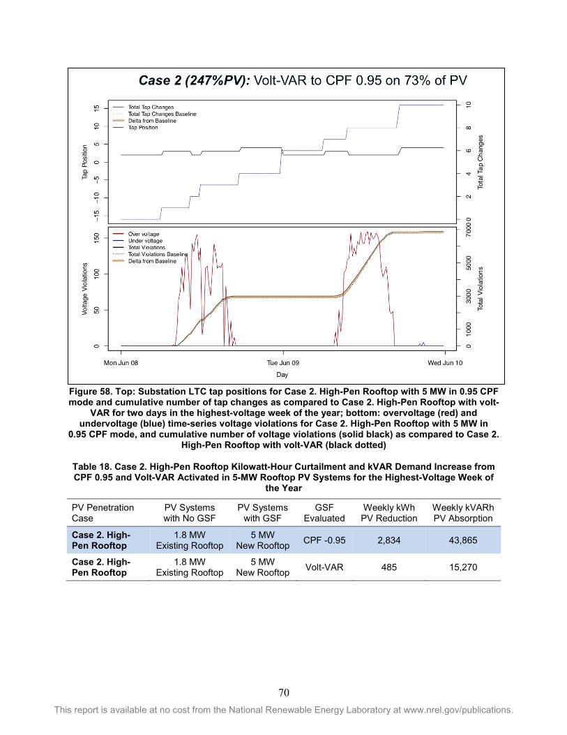
70 This report is available at no cost from the National Renewable Energy Laboratory at www.nrel.gov/publications.
Figure 58. Top: Substation LTC tap positions for Case 2. High-Pen Rooftop with 5 MW in 0.95 CPF mode and cumulative number of tap changes as compared to Case 2. High-Pen Rooftop with volt-
VAR for two days in the highest-voltage week of the year; bottom: overvoltage (red) and undervoltage (blue) time-series voltage violations for Case 2. High-Pen Rooftop with 5 MW in
0.95 CPF mode, and cumulative number of voltage violations (solid black) as compared to Case 2. High-Pen Rooftop with volt-VAR (black dotted)
Table 18. Case 2. High-Pen Rooftop Kilowatt-Hour Curtailment and kVAR Demand Increase from CPF 0.95 and Volt-VAR Activated in 5-MW Rooftop PV Systems for the Highest-Voltage Week of
the Year
PV Penetration Case
PV Systems with No GSF
PV Systems with GSF
GSF Evaluated
Weekly kWh PV Reduction
Weekly kVARh PV Absorption
Case 2. High-Pen Rooftop
1.8 MW Existing Rooftop
5 MW New Rooftop CPF -0.95 2,834 43,865
Case 2. High-Pen Rooftop
1.8 MW Existing Rooftop
5 MW New Rooftop Volt-VAR 485 15,270

71 This report is available at no cost from the National Renewable Energy Laboratory at www.nrel.gov/publications.
4.3.3 Utility and Customer Implications with 0.95 CPF/Volt-Watt and Volt-VAR/Volt-Watt
4.3.3.1 Case 1. PE-Rooftop Because volt-watt is not highly utilized in this near-future PV penetration case of adding the pending rooftop at 0.95 CPF/volt-watt and volt-VAR/volt-Watt, the energy curtailment is negligible for the latter scenario and low for the former, as shown in Table 19.
Table 19. Case 1. PE Rooftop Kilowatt-Hour Curtailment and kVAR Demand Increase from CPF 0.95/Volt-Watt and Volt-VAR/Volt-Watt activated in 550-kW rooftop PV Systems for the Highest-
Voltage Week of the Year
PV Penetration Case PV Systems with No GSF
PV Systems with GSF
GSF Evaluated
Weekly kWh PV Reduction
Weekly kVARh PV Absorption
Case 1. PE-Rooftop 1.8 MW Existing Rooftop
550 kW New Rooftop
CPF -0.95 Volt-Watt 449 4,742
Case 1. PE-Rooftop 1.8 MW Existing Rooftop
550 kW New Rooftop
Volt-VAR Volt-Watt 19 122
4.3.3.2 Case 2. High-Pen Rooftop In contrast to the previous PV penetration case in section 4.3.3.1, volt-watt frequently is activated with an additional 5 MW of PV energy added to the system in CPF 0.95/volt-watt and volt-VAR/volt-watt. The customer energy production curtailment, however, is less with volt-VAR in combination with volt-watt than with CPF 0.95 with volt-watt (see Table 20).
Table 20. Case 2. High-Pen Rooftop Kilowatt-Hour Curtailment and kVAR Demand Increase from CPF 0.95/Volt-Watt and Volt-VAR/Volt-Watt Activated in 5-MW Rooftop PV Systems for the
Highest-Voltage Week of the Year
PV Penetration Case
PV Systems with No GSF
PV Systems with GSF
GSF Evaluated
Weekly kWh PV Reduction
Weekly PV Absorption
Case 2. High-Pen Rooftop
1.8 MW Existing Rooftop
5 MW New Rooftop
CPF -0.95 Volt-Watt 4,355 42,886
Case 2. High-Pen Rooftop
1.8 MW Existing Rooftop
5 MW New Rooftop
Volt-VAR Volt-Watt 668 14,436
4.4 Annual Energy Reduction to Customers and Impact to the
Bulk System To estimate annual kilowatt-hour and percentage energy curtailment, 0.95 CPF in combination with volt-watt, as well as volt-VAR with volt-watt were run for a year.
• CPF 0.95 in combination with volt-watt results in the greatest energy curtailment to the customers.

72 This report is available at no cost from the National Renewable Energy Laboratory at www.nrel.gov/publications.
• The percentage of advanced inverters deployed in a feeder affect how much volt-watt is activated and, as a result, the energy curtailment to PV-system customers. In M34 feeder cases with the pending FITs in the model that are interconnected at unity power factor, the percent share of advanced inverters is less than the share of legacy inverters, and the energy curtailed is greater than in the case without the planned FITs.
• Volt-VAR in combination with volt-watt always results in considerably less energy curtailed to PV-system owners with grid support functions.
Regarding the impact to the utility, it is apparent that the reactive power demand at the substation increases considerably with CPF 0.95, whereas the voltage-based control volt-VAR absorbs less than the reactive power demand for both feeders, as shown in Table 21 and Table 22. Even with the use of volt-VAR, however, the overall increase in reactive power demand, in the aggregate of an entire distribution system, could impact the bulk power system and this should be further explored.
Table 21. M34 Annual Kilowatt-Hour Curtailment and kVAR Demand Increase for CPF 0.95/Volt-Watt and Volt-VAR/Volt-Watt
PV Penetration Case
PV Systems with No GSF
PV Systems with GSF
GSF Evaluated
Annual kWh PV
Reduction
Annual kVARh PV Absorption
Case 1. PE-Rooftop
1.6 MW Existing Rooftop + 1.8 MW FITs
1.8 MW New Rooftop
CPF -0.95 Volt-Watt
80,271 (3.1%) 705,818
Case 1. PE-Rooftop
1.6 MW Existing Rooftop + 1.8 MW FITs
1.8 MW New Rooftop
Volt-VAR Volt-Watt
11,268 (0.5%) 87,452
Case 1. PE-Rooftop +PE-FIT
1.6 MW Existing Rooftop
+ 7 MW FITs
1.8 MW New Rooftop
CPF -0.95 Volt-Watt
90,174 (4%) 705,833
Case 1. PE-Rooftop +PE-FIT
1.6 MW Existing Rooftop
+ 7 MW FITs
1.8 MW New Rooftop
Volt-VAR Volt-Watt
17,268 (0.7%)
112,536
Case 2. High-Pen Rooftop
1.6 MW Existing Rooftop
5.5 MW New Rooftop
CPF -0.95 Volt-Watt
318,129 (3.8%) 2,762,893
Case 2. High-Pen Rooftop
1.6 MW Existing Rooftop
5.5 MW New Rooftop
Volt-VAR Volt-Watt
49,577 (0.6%) 514,327
Case 2. High-Pen Rooftop+PE-FIT
1.6 MW Existing Rooftop
+ 7 MW FITs
5.5 MW New Rooftop
CPF -0.95 Volt-Watt
377,525 (4.5%) 2,762,995
Case 2. High-Pen Rooftop +PE-FIT
1.6 MW Existing Rooftop
+ 7 MW FITs
5.5 MW New Rooftop
Volt-VAR Volt-Watt
73,264 (0.9%)
835,225
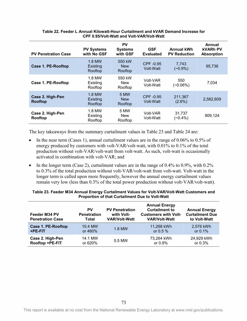
73 This report is available at no cost from the National Renewable Energy Laboratory at www.nrel.gov/publications.
Table 22. Feeder L Annual Kilowatt-Hour Curtailment and kVAR Demand Increase for CPF 0.95/Volt-Watt and Volt-VAR/Volt-Watt
PV Penetration Case PV Systems with No GSF
PV Systems with GSF
GSF Evaluated
Annual kWh PV Reduction
Annual kVARh PV Absorption
Case 1. PE-Rooftop 1.8 MW Existing Rooftop
550 kW New
Rooftop
CPF -0.95 Volt-Watt
7,743 (~0.9%) 95,736
Case 1. PE-Rooftop 1.8 MW Existing Rooftop
550 kW New
Rooftop
Volt-VAR Volt-Watt
550 (~0.06%) 7,034
Case 2. High-Pen Rooftop
1.8 MW Existing Rooftop
5 MW New
Rooftop
CPF -0.95 Volt-Watt
211,367 (2.6%) 2,582,609
Case 2. High-Pen Rooftop
1.8 MW Existing Rooftop
5 MW New
Rooftop
Volt-VAR Volt-Watt
31,737 (~0.4%) 909,124
The key takeaways from the summary curtailment values in Table 23 and Table 24 are:
• In the near term (Cases 1), annual curtailment values are in the range of 0.06% to 0.5% of energy produced by customers with volt-VAR/volt-watt, with 0.01% to 0.1% of the total production without volt-VAR/volt-watt from volt-watt. As such, volt-watt is occasionally activated in combination with volt-VAR; and
• In the longer term (Case 2), curtailment values are in the range of 0.4% to 0.9%, with 0.2% to 0.3% of the total production without volt-VAR/volt-watt from volt-watt. Volt-watt in the longer term is called upon more frequently, however the annual energy curtailment values remain very low (less than 0.3% of the total power production without volt-VAR/volt-watt).
Table 23. Feeder M34 Annual Energy Curtailment Values for Volt-VAR/Volt-Watt Customers and Proportion of that Curtailment Due to Volt-Watt
Feeder M34 PV Penetration Case
PV Penetration
Total
PV Penetration with Volt-
VAR/Volt-Watt
Annual Energy Curtailment to
Customers with Volt-VAR/Volt-Watt
Annual Energy Curtailment Due
to Volt-Watt
Case 1. PE-Rooftop +PE-FIT
10.4 MW or 460% 1.8 MW 11,268 kWh
or 0.5 % 2,576 kWh
or 0.1%
Case 2. High-Pen Rooftop +PE-FIT
14.1 MW or 620% 5.5 MW 73,264 kWh
or 0.9% 24,929 kWh
or 0.3%

74 This report is available at no cost from the National Renewable Energy Laboratory at www.nrel.gov/publications.
Table 24. Feeder L Annual Energy Curtailment Values for Volt-VAR/Volt-Watt Customers and Proportion of that Curtailment Due to Volt-Watt
Feeder L PV Penetration Case
PV Penetration
Total
PV Penetration with Volt-
VAR/Volt-Watt
Annual Energy Curtailment to
Customers with Volt-VAR/Volt-Watt
Annual Energy Curtailment Due
to Volt-Watt
Case 1. PE-Rooftop 2.3 MW or 81% 550 kW 550 kWh
or 0.06% 130 kWh or 0.01%
Case 2. High-Pen Rooftop
6.8 MW or 247% 5 MW 31,737 kWh
or 0.4% 15,513 kWh
or 0.2%
Activating volt-watt in combination with volt-VAR in the near-term PV-penetration cases results in annual energy curtailment of less than 0.5% per customer for 95% of the customers and less than 5% for the remaining 5% in both M34 and feeder L customers with volt-VAR/volt-watt activated as shown in the histogram of customer annual energy curtailment values in Figure 59.
In the longer term, PV-penetration cases that look at rooftop PV–penetration levels equal to the peak load of the feeder, the customer annual energy curtailment values for customers with volt-VAR and volt-watt remain relatively low: 87% of the customers with volt-VAR/volt-watt would experience annual energy curtailment values of 1% or less, 11% would experience between 1% and 5%, and the remaining 2% would experience curtailment values of between 5% and 10%. The histograms of annual energy curtailed for M34 and L feeders are shown in Figure 60.
Note that because PV systems in the simulations did not turn off with voltages higher than 1.1 pu voltage as they would have in the field, the simulated voltages of future PV penetration cases presented are higher than they would be expected to occur in the field. However, due to voltages being higher (versus lower) with this assumption, the impact to the metrics presented above is that they would be even lower. In the energy curtailment calculations to PV customers with GSF activated, the energy reduction from PV systems that would have been turned off due to the 1.1 pu voltage disconnection requirement in IEEE 1547-2003 is not included in the calculation. This avoids attributing the energy curtailment from PV customers that would have been disconnected in reality to the energy curtailment calculation from activating a certain GSF.

75 This report is available at no cost from the National Renewable Energy Laboratory at www.nrel.gov/publications.
Figure 59. Histogram of percent of annual energy curtailed for every customer with volt-VAR/volt-watt activated for M34 Case 1. PE-Rooftop+PE-FIT (left) and feeder L Case 1. PE-Rooftop (right)

76 This report is available at no cost from the National Renewable Energy Laboratory at www.nrel.gov/publications.
Figure 60. Histogram of percent of annual energy curtailed for every customer with volt-VAR/volt-watt activated (left) for M34 Case 2.
High-Pen Rooftop+PE-FIT, and feeder L Case 2. High-Pen Rooftop (right)
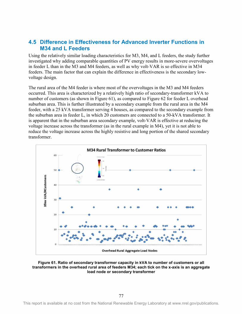
77 This report is available at no cost from the National Renewable Energy Laboratory at www.nrel.gov/publications.
4.5 Difference in Effectiveness for Advanced Inverter Functions in M34 and L Feeders
Using the relatively similar loading characteristics for M3, M4, and L feeders, the study further investigated why adding comparable quantities of PV energy results in more-severe overvoltages in feeder L than in the M3 and M4 feeders, as well as why volt-VAR is so effective in M34 feeders. The main factor that can explain the difference in effectiveness is the secondary low-voltage design.
The rural area of the M4 feeder is where most of the overvoltages in the M3 and M4 feeders occurred. This area is characterized by a relatively high ratio of secondary-transformer kVA to number of customers (as shown in Figure 61), as compared to Figure 62 for feeder L overhead suburban area. This is further illustrated by a secondary example from the rural area in the M4 feeder, with a 25 kVA transformer serving 4 houses, as compared to the secondary example from the suburban area in feeder L, in which 20 customers are connected to a 50-kVA transformer. It is apparent that in the suburban area secondary example, volt-VAR is effective at reducing the voltage increase across the transformer (as in the rural example in M4), yet it is not able to reduce the voltage increase across the highly resistive and long portion of the shared secondary transformer.
Figure 61. Ratio of secondary transformer capacity in kVA to number of customers or all transformers in the overhead rural area of feeders M34; each tick on the x-axis is an aggregate
load node or secondary transformer

78 This report is available at no cost from the National Renewable Energy Laboratory at www.nrel.gov/publications.
Figure 62. Ratio of secondary transformer capacity kVA to number of customers for all
transformers in the overhead suburban area of feeder L; each tick on the x-axis is an aggregate load node or secondary transformer
Figure 63. M4 Rural overhead secondary example with three PV systems for Case 2. High-Pen
Rooftop; red indicates no advanced inverters and blue indicates volt-VAR
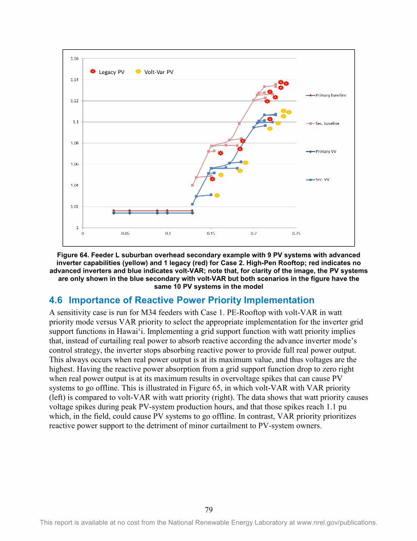
79 This report is available at no cost from the National Renewable Energy Laboratory at www.nrel.gov/publications.
Figure 64. Feeder L suburban overhead secondary example with 9 PV systems with advanced inverter capabilities (yellow) and 1 legacy (red) for Case 2. High-Pen Rooftop; red indicates no
advanced inverters and blue indicates volt-VAR; note that, for clarity of the image, the PV systems are only shown in the blue secondary with volt-VAR but both scenarios in the figure have the
same 10 PV systems in the model
4.6 Importance of Reactive Power Priority Implementation A sensitivity case is run for M34 feeders with Case 1. PE-Rooftop with volt-VAR in watt priority mode versus VAR priority to select the appropriate implementation for the inverter grid support functions in Hawai‘i. Implementing a grid support function with watt priority implies that, instead of curtailing real power to absorb reactive according the advance inverter mode’s control strategy, the inverter stops absorbing reactive power to provide full real power output. This always occurs when real power output is at its maximum value, and thus voltages are the highest. Having the reactive power absorption from a grid support function drop to zero right when real power output is at its maximum results in overvoltage spikes that can cause PV systems to go offline. This is illustrated in Figure 65, in which volt-VAR with VAR priority (left) is compared to volt-VAR with watt priority (right). The data shows that watt priority causes voltage spikes during peak PV-system production hours, and that those spikes reach 1.1 pu which, in the field, could cause PV systems to go offline. In contrast, VAR priority prioritizes reactive power support to the detriment of minor curtailment to PV-system owners.

80 This report is available at no cost from the National Renewable Energy Laboratory at www.nrel.gov/publications.
Figure 65. Case 1. PE-Rooftop with 1.8 MW of pending rooftop PV systems in volt-VAR VAR
priority mode (left) and volt-VAR watt priority mode (right)
5 Summary of Conclusions and Recommendations The simulation results presented in this report examine the effectiveness in regulating voltage as well as the impact to the utility and the customers of various inverter-based grid support functions on two Hawaiian Electric distribution substations. The distribution substation and feeder models are enhanced to add the necessary level of detail in the low-voltage secondary networks, and are run under different actual (as of year-end 2015) and future PV-penetration cases. The power-flow is solved with OpenDSS which is run via the COM interface using Python. Some of the OpenDSS inverter controls are used to model grid support functions such as volt-VAR with reactive power priority; however, CPF with VAR priority and the combination modes with volt-watt were not available in the latest version OpenDSS at the time of the simulation set-up and thus were developed in Python.
The main conclusions and recommendations drawn for the simulation cases and grid support function scenarios are as follows.
• Additional PV systems with GSF interconnected to a distribution circuit increase the impact on improving overall voltage profiles.
• Activating GSF in new PV systems has no adverse impact to legacy utility owned voltage regulation equipment (substation LTC) in terms of increasing total number of operations.
• Volt-VAR is always as effective or more effective for regulating voltages during PV-system production hours6. This is quantified by looking at the DeltaV metric, which is a measure of how much “flatter” voltages are with a given grid support function as compared to the no advanced inverters scenario during high PV-system production hours (10 a.m. to 2 p.m.).
6 Note that the volt-VAR curve settings can absorb/produce up to 0.9 power factor, whereas the default CPF absorbed 0.95 power factor.

81 This report is available at no cost from the National Renewable Energy Laboratory at www.nrel.gov/publications.
• Because volt-VAR is a voltage-based control, it provides targeted reactive power support as compared to CPF 0.95. Consequently, volt-VAR results always in:
o Less energy curtailment to the customers with advanced inverter GSF activated; and
o Less reactive power demand at the feeder head.
• Activating GSF with reactive power priority is recommended for Hawaiian Electric to avoid momentary overvoltages. When implementing the GSF with watt priority (CA Rule 21 implementation), momentary overvoltages are observed at peak PV-system production hours because reactive power support drops to zero during very high irradiance values to accommodate for real power production. Momentary overvoltages higher than 1.1 pu cause PV systems to disconnect according to IEEE 1547-2003, which would be detrimental to PV-system customers and to the utility.
• Even if the use of volt-VAR results in less increase of reactive power demand at the feeder level when compared to CPF 0.95, the increase in reactive power demand in the aggregate of an entire distribution system with very high penetrations of volt-VAR could impact the bulk power system. In the case of Hawai‘i, it is recommended that the potential impact of GSF in the transmission system be further explored.
• The activation of volt-watt when combined with CPF and volt-VAR relies on the effectiveness of CPF or volt-VAR first to regulate voltage before it reduces power output to protect against voltage excursions.
• Activating volt-watt in combination with volt-VAR in the near-term PV-penetration cases—which model all the pending execution interconnection of PV systems with advanced inverters in the two high-penetration feeders included in this study—results in a minor increase in the amount of reductions in PV-energy production (0.06% to 0.5% of annual energy reduction for all pending rooftop PV customers with volt-VAR/volt-watt activated, with 0.01-0.1% attributed to volt-watt).
• Activating volt-watt in combination with volt-VAR in the long-term PV-penetration cases—which model a PV penetration of rooftop PV equal to the peak load of the feeder—results in annual energy curtailment values in the range of 0.4% to 0.9% for all pending rooftop PV customers with volt-VAR/volt-watt activated, with 0.2-0.3% from volt-watt. Volt-watt in the longer term is called upon more frequently. However, the annual energy curtailment values remain very low (less than 0.3% of the total power production without volt-VAR/volt-watt).
• Activating volt-watt in combination with volt-VAR in the near-term PV-penetration cases results in annual energy curtailment of less than 0.5% per customer for 95% of the customers and less than 5% for the remaining 5% of the customers.
• In the longer-term PV-penetration cases that examine rooftop PV–penetration levels equal to the peak load of the feeder, the annual customer curtailment values for customers with volt-VAR and volt-watt remain relatively low: 87% of the customers with volt-VAR and volt-watt would experience annual energy curtailment values of less than 1%, 11% of between 1% and 5%, and the remaining 2% of customers would experience energy curtailment values between 5% and 10%.

82 This report is available at no cost from the National Renewable Energy Laboratory at www.nrel.gov/publications.
• Enabling volt-watt might cause small reductions in PV-energy production for some customers, but it will result in more total customers being able to interconnect PV systems, thus the net effect will allow for more cumulative renewable-energy production. By providing a backstop against voltages above ANSI C84.1 levels, enabling volt-watt and volt-VAR sooner will result in removing high voltage as a barrier for interconnecting greater levels of distributed PV systems.
• Adding PV systems with grid support functions such as CPF and volt-VAR to the baseline (distribution feeder conditions as of year-end 2015) does not fix existing voltage violations due to the impact of existing legacy PV systems already interconnected with no grid support functions.
• Adding more-accurate representations of secondary circuits is a key to capturing voltages at the point of common coupling and estimating reductions in PV-energy production. In the case of O’ahu island feeders, voltage drops/increases of 5% are observed across the secondary of service transformers and secondary network, and this would have not been captured with the generic star low-voltage network modeling approach (a dedicated line of the same length and conductor type from the service transformer to every customer meter).
• GSF within the context of IEEE 1547 Standards and Rule 14H in Hawai‘i are specified at the customer meter or PCC, which is what is modeled in the VROS Project. Behind-the-meter voltage rise per the National Electric Code can be greater than the ANSI C84.1 limits that utilities maintain at the PCC. To avoid unnecessary curtailment from activating GSF, PV installers and system designers must account for the voltage rise up to the inverter terminals.
Some of the caveats and limitations to the current work are as follows.
• The current PV systems do not turn off at 1.1 pu voltage as they would in the field according to IEEE 1547. This causes overall higher voltages in the range of the voltage control based grid support functions such as volt-VAR and volt-watt. As such, these functions are called upon more often than they would have if feeder voltages were not as high. Because the VROS project simulated voltages higher than 1.1 pu, the curtailment for PV systems above 1.1 pu was not counted as curtailment associated to a grid support function, however, it is likely that volt-VAR and volt-watt in the simulation were activated more often than it would have been observed in the field.
• Due to the time constraints of the VROS project, the volt-watt algorithm used in combination with CPF and volt-VAR was programmed outside the OpenDSS software. It was observed that in clear-sky days, the volt-watt algorithm used in this project resulted in over-curtailment of up to 10% more of the real power value expected for a 15 min time-step, and over-corrected voltages to the 1.05 pu range in some cases. This implies that the volt-watt annual energy curtailment values are slightly over-estimated. It is suspected that more development is needed in the empirically derived damping factor used in the volt-watt algorithm to improve simulation convergence accuracy.
• Secondary low-voltage networks were added to M34 feeders but there are no voltage measurements below the service transformers to validate the voltages simulated at the household level. Voltages, however, are validated at the secondary terminals of the distribution service transformer.
83 This report is available at no cost from the National Renewable Energy Laboratory at www.nrel.gov/publications.
• The M34 feeders do not have load diversity; the same substation gross-load profile drives all the loads represented in the system. During PV-system producing hours, the main driver of voltage changes comes from PV systems and not from the load, and the metrics quantified in this study (e.g., DeltaV, kWh reduction) mainly are dependent on the voltage profiles during high PV-system generation hours, so this limitation is not expected greatly affect the results.
• Secondary low-voltage circuits are modeled up to the customer meter, but further voltage drop/rise could occur between the meter and the PV system point of interconnection. This is consistent with the reference point of applicability where the interconnection and interoperability performance requirements are required to be met. The volt-watt function proposed by the Companies initiates reduction in real power when the voltage at the inverter terminals crosses 1.06 pu. Therefore, PV system installers and system designers should account for the additional voltage drop up to the inverter terminals. Note however, that this is a field-installation issue and does not affect the modeling in this report.
• Current PV-penetration cases include all PV systems interconnected with the ability to export (as in net-energy-meter or customer-grid-supply tariffs offered by Hawaiian Electric); however, some systems are interconnected in a non-exporting agreement (customer self-supply). The implications of having non-exporting PV customers are not modeled in this study and could impact daytime and nighttime voltage profiles.
• The QSTS was run at 15-minute time steps and, as such, the considerations of impact of GSF to utility LTC operations are relative to the 15-minute time step but might not reflect all of the LTC operations because the load tap changer can regulate voltage at a 30-second resolution. Two days for feeder M34 were run with a 15-second time step, and there were no additional LTC operations observed at the smaller simulation time step as compared to the 15-minute time step results.
• The project did not consider optimizing the current utility voltage regulating equipment (substation load tap changers in the case of Hawaiian Electric) controls. The LTC in M34 was changed to reverse setting “lock” to prevent undervoltages, but the optimal control strategy for the LTCs under high PV penetration should be further explored. Note that this would only help reduce the impacts to both customer and utility.
• The study doesn’t consider other voltage management solutions (e.g., centralized integrated volt-VAR, decentralized distributed voltage support). Further investigation of the optimal solution for voltage management and how new technologies will integrate with distributed inverter grid support functions should be performed.
6 Future Work NREL is supporting Hawaiian Electric in its advanced photovoltaic inverter voltage support pilot deployment project (advanced inverter pilot project). As part of the scope of the advanced inverter pilot project, Hawaiian Electric has extended an offer to some number of queued net energy metering PV customers whose systems are not able to be installed due to expected high-voltage issues. The offer includes an option to use advanced inverters with voltage support functions activated. These customers otherwise would not have inverter-based voltage support functions activated and would have to wait for circuit upgrades—and, in some cases, would have

84 This report is available at no cost from the National Renewable Energy Laboratory at www.nrel.gov/publications.
to pay for circuit upgrades before installation. Approximately 30 customers are now enrolled in the advanced inverter pilot project and the pilot PV systems are being installed at the time of the writing of this report.
NREL is providing support for the planning, execution, and analysis of the pilot project. As part of the scope of the advanced inverter pilot project, there is a specific task dedicated to the validation of the VROS Project with field data. The field data will be used to validate the VROS Project models, and in particular to validate the service voltage drop from secondary transformers to the point of interconnection of the PV inverters, as well as the response of multiple inverters in regulating feeder voltage. The updated VROS Project models then will be used to extrapolate from the field data to higher penetration levels of grid-supportive inverters and annual voltage profiles and kWh-production estimates will be updated.
Recently, the U.S. Department of Energy has designated the VROS and advanced inverter pilot Projects as “high-impact” projects. The additional scope includes the evaluation of the impact of customer-sited storage, enabling customer electric water-heater control, and electric vehicles in the feeder voltage management schemes. For the water-heater control analysis, NREL is leveraging the AMI customer data used in this study to extract occupancy patterns and estimate electric water-heater profiles.
The field data from the advanced inverter pilot project is expected to calibrate and validate the findings of this VROS Project, and the added scope from the “high-impact” expansion will address some of the limitations described above (such as the secondary low-voltage networks being modeled up to the PCC and the implications of having non-exporting PV customers with storage).
Other potential future work that derives from the findings of the VROS project is described below.
• Study the impact of increased reactive power demand from activating grid support functions in the transmission system. What is the technical and economic impact to the transmission system of increasing reactive power demand for grid support functions?
• Future deployments of PV systems with grid support functions can’t mitigate the current impacts of the high number of PV systems already installed in the Hawaiian Electric distribution system. As such, other voltage management solutions should be explored in parallel to interconnecting future PV with grid support functions. Some of the unanswered questions are listed below.
o What is the optimal control for existing utility legacy voltage regulating equipment? Advanced centralized integrated volt-VAR solutions as well as decentralized grid-edge software control algorithms are being proposed to improve the voltage management of current voltage-regulating equipment in distribution systems with high PV penetrations [14].
o What is the optimal design for regulating voltage using legacy voltage regulating equipment, PV systems with GSF, and centralized and decentralized grid-edge hardware and software volt-VAR control? This research question should be studied from both the technical and cost-benefit perspectives.

85 This report is available at no cost from the National Renewable Energy Laboratory at www.nrel.gov/publications.
References [1] A. Hoke et al., “Hawaiian Electric Advanced Inverter Grid Support Function Validation
and Analysis,” Technical Report NREL/TP-5D00-67485, December 2016. [2] A. Nagarajan, A. Nelson, K. Prabakar, A. Hoke, M. Asano, R. Ueda, S. Nepal, “Network
Reduction Algorithm for Developing Distribution Feeders for Real-Time Simulators,” IEEE Power and Energy Society General Meeting, July 2017.
[3] A. Nelson, K. Prabakar, A. Nagarajan, S. Nepal, A. Hoke, M. Asano, R. Ueda, E. Ifuku, “Power Hardware-in-the-Loop Evaluation of PV Inverter Grid Support on Hawaiian Electric Feeders,” 2017 IEEE Innovative Smart Grid Technologies Conference (ISGT), April 2017.
[4] Electric Power Research Institute, “Analysis to Inform CA Grid Integration: Methods and Default Settings to Effectively Use Advanced Inverter Functions in the Distribution System,” Technical Report 3002007139 (Palo Alto, CA: 2015).
[5] B. York, “Arizona Public Service Solar Partner Program Advanced Inverter Demonstration Results,” 3002011316 EPRI Final Report, May 2017.
[6] F. Ding et al., “Voltage Support Study of Smart PV Inverters on a High-Photovoltaic Penetration Utility Distribution Feeder,” 2016 IEEE 43rd Photovoltaic Specialists Conference (PVSC), Portland, Oregon, 2016, pp. 1375–1380.
[7] F. Ding et al., “Photovoltaic Impact Assessment of Smart Inverter Volt-VAR Control on Distribution System Conservation Voltage Reduction and Power Quality,” Technical Report NREL/TP-5D00- 67296, December 2016.
[8] “IEEE Standard 1547: Standard for Interconnecting Distributed Resources with Electric Power Systems,” IEEE, 2003.
[9] “P1547/D6.7.2, May 2017—IEEE Draft Standard for Interconnection and Interoperability of Distributed Energy Resources with Associated Electric Power Systems Interfaces,” IEEE, 2017.
[10] “OpenDSS,” Electric Power Research Institute. https://sourceforge.net/projects/electricdss/.
[11] Python Software Foundation. Python Language Reference, version 2.7. Available at http://www.python.org.
[12] “Reference Guide the Open Distribution System SimulatorTM (OpenDSS),” Electric Power Institute OpenDSS Manual, March 2016.
[13] ANSI Standard C84.1-1995 Electric Power Systems and Equipment-Voltage Ratings (60 Hz) Table 1 "Standard Normal System Voltages and Voltage Ranges."
[14] R. Moghe, D. Tholomier, D. Divan, J. Schatz and D. Lewis, "Grid Edge Control: A new approach for volt-var optimization," 2016 IEEE/PES Transmission and Distribution Conference and Exposition (T&D), Dallas, TX, 2016, pp. 1-5.

86 This report is available at no cost from the National Renewable Energy Laboratory at www.nrel.gov/publications.
Appendix A. Model Conversion and Validation Data Conversion from Synergi to OpenDSS The conversion software code is programmed in Python and is structured such that properties for each instance of a Synergi object are collected for all objects in the feeder file in XML format, and then operated on via syntax or mathematical conversions to create a corresponding OpenDSS element, associated DSS file, and master circuit file.
Specifically, the conversion process reads the XML file and identifies, collects, and categorizes objects and their parameters for all object blocks within the XML file. As shown in Figure 66, the object blocks are identified by the symbol “<” with six space characters of indentation from the margin. After the object type is identified, a function defined for that object type is called and the values for each property are collected. The called function then assigns the collected property values to the container for that object type. In the functions, the values are not altered and the names of each object are kept the same as assigned in the Synergi XML file, which assists in the debugging process. The next step in the conversion process is to create objects in the OpenDSS script using the collected Synergi objects and their properties. A view of the syntax identification process is presented in Figure 66.
Figure 66. Diagrammatic view of Synergi to OpenDSS model conversion depicting the syntax identification process
The process of converting objects in Synergi to the equivalent objects in the OpenDSS script is not always a direct one-to-one conversion. Object types that exist in Synergi do not always exist in OpenDSS and vice versa. This also is true for the properties of objects. Switches, reclosers,

87 This report is available at no cost from the National Renewable Energy Laboratory at www.nrel.gov/publications.
and fuses are not separate objects in OpenDSS. The conversion tool creates short, low-impedance lines with switching capabilities for these components.
Finally, the converted OpenDSS script is written to a master file, and separate DSS files for each object type are created. The master file initiates a new circuit that creates a voltage source and source bus. The voltage and source impedances are specified based on data from the Synergi model. The master file also redirects to DSS component files containing scripts for the different object types separated into different categories.
Time-Series Validation Figure 67 through Figure 75 show the real power and voltage at the nine Grid 20/20 measurement locations in Mikilua 3 and 4 feeders. For the most part, the real power matches remarkably well with the measured load at the secondary transformer locations, in particular when there is PV at customers connected that point. In Figure 69, Figure 74 and Figure 75, the real power is significantly greater in the first two and lower in the latter one, which is expected when comparing field load data with estimated model data. The same applies to the spikier profile in the field data, as compared to the smoother gross load profile. As mentioned, however, the variability of PV is fairly well-represented from the PV profile estimated in the data-processing effort previously described. When comparing voltages at the measurement locations, the voltage profile of the OpenDSS model matches the field data.
Note that the other very important operating variable that can be validated is that the load tap changer in the model is behaving very much like it does in the field, as the step changes and voltage profiles driven by the LTC regulation in both field and modeled voltages can be observed. Another important clarification is that the OpenDSS model used to reproduce these results does not have the secondary transformers and, as such, the figures are comparing primary voltage in the model to secondary voltage in the field. Thus, the model results will more closely match the field data when the secondary transformers are added.

88
This report is available at no cost from the National Renewable Energy Laboratory at www.nrel.gov/publications.
Figure 67. Power (top) and voltage (bottom) time-series comparison between Grid 20/20 measurements and OpenDSS model at M3 transformer 1400 for September 16–17, 2015
Figure 68. Power (top) and voltage (bottom) time-series comparison between Grid 20/20 measurements and OpenDSS model at M3 transformer 1413 for September 16–17, 2015

89
This report is available at no cost from the National Renewable Energy Laboratory at www.nrel.gov/publications.
Figure 69. Power (top) and voltage (bottom) time-series comparison between Grid 20/20 measurements and OpenDSS model at M4 transformer 1403 for September 16–17, 2015
Figure 70. Power (top) and voltage (bottom) time-series comparison between Grid 20/20 measurements and OpenDSS model at M4 transformer 1404 for September 16–17, 2015

90
This report is available at no cost from the National Renewable Energy Laboratory at www.nrel.gov/publications.
Figure 71. Power (top) and voltage (bottom) time-series comparison between Grid 20/20 measurements and OpenDSS model at M4 transformer 1414 for September 16–17, 2015
Figure 72. Power (top) and voltage (bottom) time-series comparison between Grid 20/20 measurements and OpenDSS model at M4 transformer 1579 for September 16–17, 2015
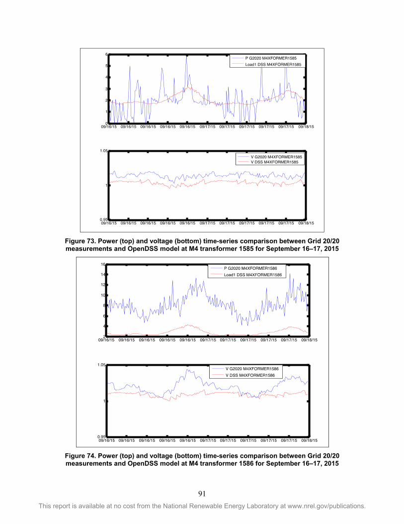
91
This report is available at no cost from the National Renewable Energy Laboratory at www.nrel.gov/publications.
Figure 73. Power (top) and voltage (bottom) time-series comparison between Grid 20/20 measurements and OpenDSS model at M4 transformer 1585 for September 16–17, 2015
Figure 74. Power (top) and voltage (bottom) time-series comparison between Grid 20/20 measurements and OpenDSS model at M4 transformer 1586 for September 16–17, 2015
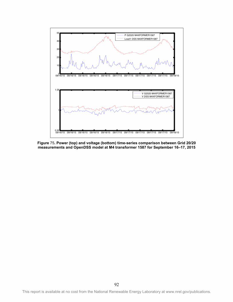
92 This report is available at no cost from the National Renewable Energy Laboratory at www.nrel.gov/publications.
Figure 75. Power (top) and voltage (bottom) time-series comparison between Grid 20/20 measurements and OpenDSS model at M4 transformer 1587 for September 16–17, 2015

93 This report is available at no cost from the National Renewable Energy Laboratory at www.nrel.gov/publications.
Appendix B. Simulation Results Plots M34 Case 1 Voltage Profiles for CPF 0.95/Volt-Watt and Volt-VAR/Volt-Watt
Figure 76. Case 1. PE-Rooftop CPF 0.95/volt-watt (left) and volt-VAR/volt-watt (right) customer
meter voltages for M34 feeders for the highest-voltage week of the year with no advanced inverters
Figure 77. Case 1. PE-Rooftop+PE-FIT CPF 0.95/volt-watt (left) and volt-VAR/volt-watt (right) customer meter voltages for M34 feeders for the highest-voltage week of the year with no
advanced inverters
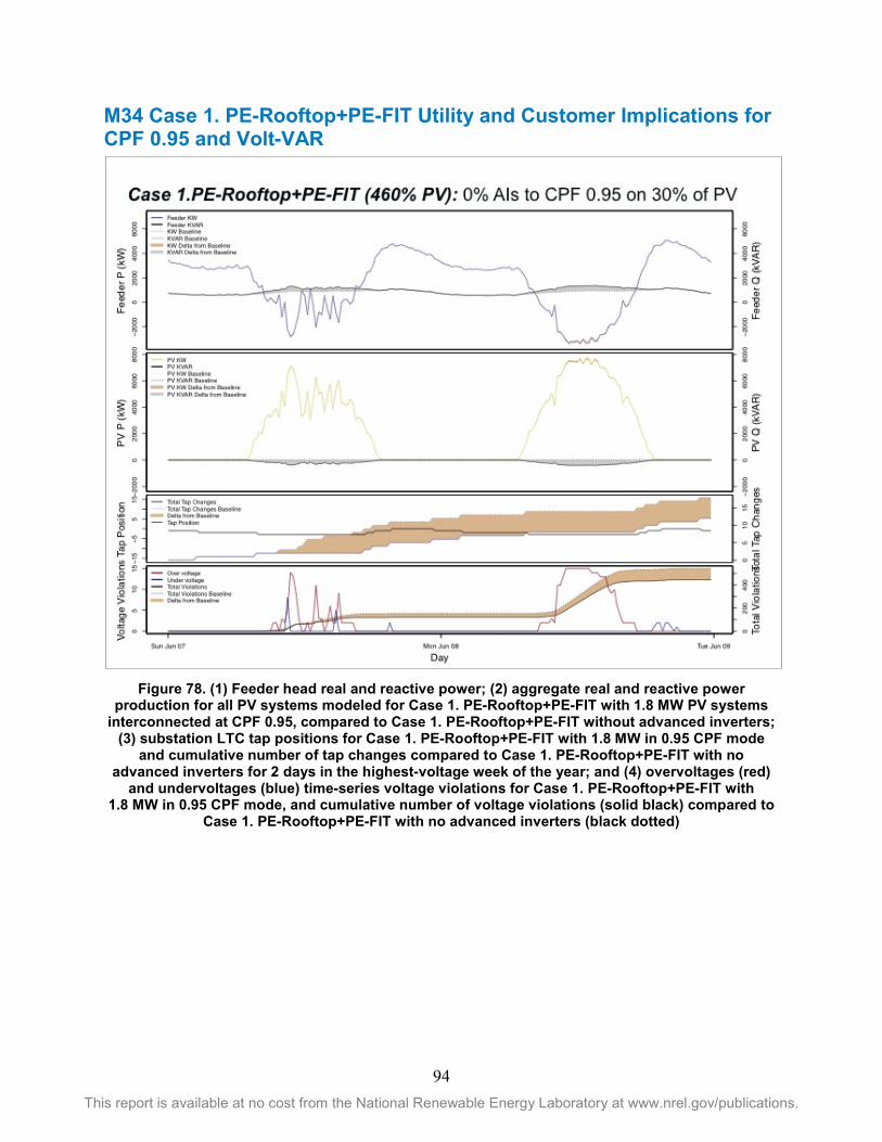
94 This report is available at no cost from the National Renewable Energy Laboratory at www.nrel.gov/publications.
M34 Case 1. PE-Rooftop+PE-FIT Utility and Customer Implications for CPF 0.95 and Volt-VAR
Figure 78. (1) Feeder head real and reactive power; (2) aggregate real and reactive power
production for all PV systems modeled for Case 1. PE-Rooftop+PE-FIT with 1.8 MW PV systems interconnected at CPF 0.95, compared to Case 1. PE-Rooftop+PE-FIT without advanced inverters;
(3) substation LTC tap positions for Case 1. PE-Rooftop+PE-FIT with 1.8 MW in 0.95 CPF mode and cumulative number of tap changes compared to Case 1. PE-Rooftop+PE-FIT with no
advanced inverters for 2 days in the highest-voltage week of the year; and (4) overvoltages (red) and undervoltages (blue) time-series voltage violations for Case 1. PE-Rooftop+PE-FIT with
1.8 MW in 0.95 CPF mode, and cumulative number of voltage violations (solid black) compared to Case 1. PE-Rooftop+PE-FIT with no advanced inverters (black dotted)

95 This report is available at no cost from the National Renewable Energy Laboratory at www.nrel.gov/publications.
Figure 79. (1) Feeder head real and reactive power; (2) aggregate real and reactive power
production for all PV systems modeled for Case 1. PE-Rooftop+PE-FIT with 1.8 MW PV systems interconnected at volt-VAR, compared to Case 1. PE-Rooftop+PE-FIT without advanced inverters;
(3) substation LTC tap positions for Case 1. PE-Rooftop+PE-FIT with 1.8 MW in volt-VAR mode and cumulative number of tap changes compared to Case 1. PE-Rooftop+PE-FIT with no
advanced inverters for 2 days in the highest-voltage week of the year; and (4) overvoltages (red) and undervoltages (blue) time-series voltage violations for Case 1. PE-Rooftop+PE-FIT with 1.8 MW in volt-VAR mode, and cumulative number of voltage violations (solid black) compared to
Case 1. PE-Rooftop+PE-FIT with no advanced inverters (black dotted)

96 This report is available at no cost from the National Renewable Energy Laboratory at www.nrel.gov/publications.
Feeder L Case 1. PE-Rooftop Voltage Profiles for CPF 0.95/Volt-Watt and Volt-VAR/Volt-Watt
Figure 80. Case 1. PE-Rooftop CPF 0.95/volt-watt (left) and volt-VAR/volt-watt (right) customer
meter voltages for feeder L for the highest-voltage week of the year with no advanced inverters