Policy Research Working Paper 8304

Simulating Pension Income Scenarios with penCalc

An Illustration for India’s National Pension System

Renuka SaneWilliam Price

Finance, Competitiveness and Innovation Global Practice GroupJanuary 2018

WPS8304P

ublic

Dis

clos

ure

Aut

horiz

edP

ublic

Dis

clos

ure

Aut

horiz

edP

ublic

Dis

clos

ure

Aut

horiz

edP

ublic

Dis

clos

ure

Aut

horiz

ed

Produced by the Research Support Team

Abstract

The Policy Research Working Paper Series disseminates the findings of work in progress to encourage the exchange of ideas about development issues. An objective of the series is to get the findings out quickly, even if the presentations are less than fully polished. The papers carry the names of the authors and should be cited accordingly. The findings, interpretations, and conclusions expressed in this paper are entirely those of the authors. They do not necessarily represent the views of the International Bank for Reconstruction and Development/World Bank and its affiliated organizations, or those of the Executive Directors of the World Bank or the governments they represent.

Policy Research Working Paper 8304

This paper is a product of the Finance, Competitiveness and Innovation Global Practice Group. It is part of a larger effort by the World Bank to provide open access to its research and make a contribution to development policy discussions around the world. Policy Research Working Papers are also posted on the Web at http://econ.worldbank.org. The authors may be contacted at willprice@worldbank.org.

This paper sets out initial results from a new modeling exer-cise for Defined Contribution (DC) pensions. It develops a package called penCalc based on the open source software language R, which is popular in the academic and modeling communities. All the coding is made freely available. The tool is illustrated for India’s DC National Pension System. The aim is not to present the perfect model for India, but to show how the tool works so that policy makers and regulators can see its potential advantages and develop it for their own uses. It generates scenarios for future assets and income dependent on user-defined and changeable

assumptions for asset returns, contributions, wages, years in the labor force, and annuity prices, among other parameters. Assumptions can be tailored to different countries and user determined scenarios. Many extensions could be developed, which will be the subject of future work. The international context is highlighted through similar modeling by regu-lators and pension funds in other jurisdictions. Some of these are more complex or complete than the results in this paper, but by explaining the initial model and making the coding freely available, the authors provide a powerful yet simple and low-cost tool to be adopted and adapted.

Simulating Pension Income Scenarios with penCalc:

An Illustration for India’s National Pension System

Renuka Sane William J. Price∗

JEL Code: C63; D15; G11; G17; G18; G23; J11; J26; J46

Keywords : pensions, pension funds, retiremnet income, forecasting, simulations, India,

stock market, bond market, government bonds, equity markets, annuities

∗Renuka Sane is an Associate Professor at the National Institute of Public Finance and Policy, New Delhi and William Price is a Senior Financial Sector Specialist at the World Bank Group, Washington DC. Corresponding authors’ email renuka@saner.org.in. We would like to acknowledge the support of the FIRST Initiative in funding the engagement with India’s Pension Fund Regulatory and Development Authority during which the work in this paper was completed. We thank Arjun Gupta for research assistance. The authors are very grateful for comments received by Michael Hafeman, Evan Inglis, Mitchell Wiener, Montserrat Pallares-Miralles, Kamer Karakurum Ozdemir and Fiona Stewart on earlier versions and from the staff of the Pension Fund Regulatory and Development Authority in India. Errors and omissions remain solely the responsibility of the authors.

1 Introduction

Modeling pension outcomes is a critical part of good policy design for a pension system.

It is useful in the initial design phase - for example to ensure contributions are sufficient

to achieve a desired outcome and to see how the different pillars of a pension system

will combine to provide an overall income (Antolin, 2009; Stewart, 2014; Price, Ashcroft,

and Hafeman, 2016). It is also useful to update existing systems - for example adjusting

retirement ages to counteract rising longevity, or reviewing all parameters if long-run

returns or interest rates have fallen - as they have for many countries since the Global

Financial Crisis.

This paper sets out a new model for pension outcomes called penCalc. It is illustrated for

India’s National Pension System to give a real-world example - and to show the impact

of changing some of the main parameters. The aim is not to produce the perfect forecast

for pension payouts in India, but to show how the model works and discuss potential

assumptions and scenarios. A feature of the model is that the key assumptions can be

simply chosen by the user - which makes it particularly flexible in exploring different

scenarios within a country, as well as being tailored to many different countries.

While members can also benefit from scenarios for projections of pension outcomes - so

that they can develop a sense of likely retirement income and understand in broad terms

the impact of changing contributions, the model set out in this paper is designed for policy

makers and regulators. There is scope for the results to be used to help with member

communication if a user-friendly interface is added to allow a user to alter some key

parameters and see the results but without engaging directly with the model presented

here.

The model was developed as part of a project for the Indian Pension Regulatory and

Development Fund (PFRDA) funded by the FIRST initiative.1 As far as the authors

know it is the first such paper that publishes the coding behind the results so that others

can use the approach. While there are many extensions that can be made to the model

presented below (and these will be the subject of future work) the aim is that by showing

how simple yet powerful the tool can be - and giving free access to the coding - it provides

new opportunities for countries and organizations who may find more costly approaches

or proprietary “black-box” models do not meet their resources or needs.

1The Financial Sector Reform and Strengthening Initiative, FIRST, is a multi-donor grant facility thatprovides short- to medium-term technical assistance to promote sounder, more efficient and inclusivefinancial systems. www.firstinitiative.org

2

Part 2 of the paper sets out some existing international examples of modelling to provide

context and help explain the approach taken in this work. There is an inevitable trade-off

between complexity and usability - particularly if the aim is to allow regulators and policy

makers to have a tool with which they can work directly in order to proactively explore

policy options. Part 3 then introduces the Indian DC pension pillar that was modeled.

Part 4 reviews the drivers of the pension performance. Part 5 provides an overview of

the model. Part 6 sets out the results. Part 7 then concludes and suggests a range of

extensions to the current model that could be taken forward in future work.

2 Modeling pension outcomes for policy makers and

individuals

Modeling investment outcomes for pension fund and other investors has received a vast

amount of attention. Historically, those running Defined Benefit funds have been sig-

nificant users of modeling - to determine investment strategies, actuarial modeling to

understand and project liabilities - and in some cases to bring both elements together

in explicit asset-liability modeling to ensure their investment strategies are working to

deliver the pension promised by the plan.

While Defined Contribution plans still use investment modeling tools, and some have

been trying to take the lessons of Defined Benefit based asset-liability modeling into their

approach, the shift to Defined Contribution pensions puts a much higher premium on

understanding the likely outcomes from a given path of contributions and investments

and even more importantly to understanding the range of outcomes. Hybrid approaches,

or those that have a target retirement income butnot necessarily a full guarantee, also

need to show potential benefits and potential risks. Such approaches have been a source

for growth in ways to explain and model retirement benefits in recent years (Ionescu and

Yermo, 2014; Stanko, 2015).

This is a critical area of research because there can be huge differences in outcomes across

cohorts of pensioners based simply on when they joined and exited a system. Cannon

and Tonks (2004) take identical contribution rates and contribution durations over time

and simply alter when a person starts contributing to and exits a system. This shows the

impact of different annuity rates at exit and different investment returns (under different

investment strategies) during accumulation.

They show very large difference in retirement income despite the individuals being in all

3

Figure 1 The impact of different investment strategies and annuity rates at retirementon replacement rates over time for otherwise similar individuals over time.

Source: Cannon and Tonks (2004)

other respects identical. This is shown in Figure 1 which highlights the impact of the dif-

ferent investment strategies over time interacting with changing annuity factors over time.

There are many contributions to the literature that look at the contribution of different

potential asset allocations over time to final pension outcomes - both static differences

in the share of equities and bonds for example, and dynamic or lifecycle/life-styling rules

that shift the asset allocations from higher return assets when pension contributors are

relatively young and into more conservative assets allocations (more government bonds)

as pension members approach retirement age (Antolin, Payet, and Yermo, 2010).

As set out later in the paper, the tool also allows broken career histories to be modeled,

as well as shorter working lives and any wage or contribution level - as well as lower

densities of contribution each year by reducing the contribution level to illustrate the

impact of labor market experience more typical of informal sector workers (known as the

unorganized sector in India).

Figure 1 shows how outcomes change over time for a given country. It is also possible

to show the distribution of outcomes for a common time-period to illustrate the range of

uncertainty. Figure 2 shows the range of potential outcomes when there is uncertainty

over the key parameters such as investment returns, inflation, the interest rate or discount

rate used in annuity calculations, life expectancy and labor market attachment (Antolin

and Payet, 2010) in work that also illustrates a wide range of other methods to model

4

Figure 2 Histogram of Retirement Income Relative to Final Salary

and illustrate uncertainty - but being based on a proprietary model is not available for a

country to simply obtain and adapt. A detailed comparison of the approach in this work

compared to that in the current paper is not included here as this paper aims to introduce

the overall tool, but a more detailed compare and contrast, with the implications and

trade-offs particularly when data are lacking could be the subject of future work.

Ultimately it is important to look at all aspects affecting retirement from labor market

experience based on education and wage profile over time (flatter for lower skilled/low

income workers, steeper and then tailing off for higher income/higher education workers)

through to investment returns, contribution levels and retirement ages.

In addition to the work by Antolin and Payet cited above Dowd and Blake (2013) provide

an extremely useful examination of the key factors that should ideally be included in a

retirement income model - and show how varying the various parameters affects the out-

comes. Their approach shows the relative benefit of a 1%-point increase in contributions

to an extra year of contributions and one year less of contributions. Critically, they also

show the results using stochastic investment returns so that one is able to see the average

or expected return and the range of other outcomes at different levels of significance (for

example the expected bottom 5% of outcomes compared to the top 5% of outcomes).

5

Figure 3 Impact of different decisions on replacement rates

Source: Kevin Dowd and David Blake, PensionsMetric modeling, Cass Business School

This modeling is very rich, but also more demanding in terms of data needed to run it.

Moreover, it is also a proprietary model and hence not available for general use. Their

work includes a very useful and rigorous “best practice” template of all the assumptions

and parameters that should be modeled. Many, but not all, are included in this paper.

Future work will extend the areas covered but the aim at this stage is to illustrate the

model and make the code freely available to stimulate interest in the area and provide a

practical tool that regulators could use and develop rather than wait until all the elements

are included, which was beyond the scope of the initial project.

Other approaches aim to embed the examination of outcomes in a fully calibrated macroe-

conomic model so that contributions of labor and capital market dynamics and other

parameters can be explored in the context of an explicit model for GDP growth (Hoyo,

Alonso, and Tuesta, 2015). These analyses aim to draw out the important underlying

dynamics of labor force participation and unemployment in determining the likely aver-

age pensions for different cohorts over time. They then allow different policy simulations

to be undertaken. Again, such modeling is very powerful and a useful addition to the

literature - but may be challenging for all regulators and policy makers to use easily.

Finally, there is a set of approaches that aim to focus more on the individual and pro-

vide tools for them to understand the potential outcomes they may face. They show

how outcomes could vary - and the impact of changing a behavior such as the level or

frequency of contributions or the retirement age. The regulator in Chile (SBS) has taken

a leading role in this type of work and includes tools on its website that show members

6

Figure 4 Output from the Chilean regulator retirement income simulator

Antolin and Fuentes (2012) based on Chilean Pension Supervisor simulation tool

the expectation for their retirement income (see Figure 4).

The figure shows the output (in Spanish) once an individual has put in various parameters.

The output highlights the monthly pension one could expect if retiring at 65 on a central,

optimistic and pessimistic case. It compares that to a (user entered) desired monthly

pension and then provides a probability that the person will meet their desired pension -

in the example shown that probability is 54%. It then shows these figures in a bar chart

and how each of them would change if the person retired at 68 rather than 65. Finally,

it provides some advice in a text box on what to do to increase retirement income -

restating the option of retiring later, or increasing how often a person contributes. As

explained below the model in this paper is able to illustrate the impact of these features

in a number of ways.

An interesting recent example of combining both the policy design and member projec-

tion aspects of such modeling has been shown by the National Employment Savings Trust

(NEST) in the UK. It was faced with the task of designing its investment strategy under

reforms introduced in the UK to auto-enroll workers directly into pension plans (NEST

7

Figure 5 How the Foundation Phase reduces the risks of poor outcomes for NESTinvestors

Source: National Employment Savings Trust (NEST)

2012). NEST had to tackle the issue that if it used a typical lifecycle investment model

as was the industry standard, but that there was an (unpredictable) stock market crash

in the early years of a person contributing to a pension, people might then opt-out of

pensions due to one bad experience. So NEST used modeling of investment returns with

Monte Carlo simulations to generate a probability density function for potential outcomes

to explore different strategies. The modeling showed that introducing an innovative foun-

dation phase into the standard lifecycle strategy could dramatically reduce the likelihood

of a negative outcome but with a relatively small cost in terms of expected returns over

a full lifetime. This led NEST to develop its current default investment strategy - and

also to use the results to create simple pictures for members to (potentially) understand

likely outcomes (Figure 5).

All the approaches highlighted above require a decision on the “right” inputs for the key

parameters. If the exercise includes past history then actual values can of course be en-

8

Figure 6 Investment Returns for Equities, Bonds and Bill 1900-2017

Source: Dimson, Marsh, and Staunton (2017)

tered. But for the future, assumptions must be made. These are inherently difficult given

that actual returns can vary greatly within countries over time and between countries.

One key message for using the tool is to explore a range of scenarios - and to engage

fully with the potential distribution of outcomes that are generated by any stochastic

simulation tool. An excellent source of returns data is provided by the London Business

School-Credit Suisse Global Investment Return Yearbook. This provides real return data

for equities, government bonds and government Treasury bills for 23 countries over the

period 1900-2016. The key averages are shown in Figure 6 for the whole time period and

two sub-periods: one a period of strong equity returns and the other the period 2000-2016

in which equities under-perform bonds.

Section 4, below reviews the historic returns of the main variables and the assumptions

chosen. For equities, the historic returns in India have been very high, with an equity

risk premium over government bonds of 9%. This is used to generate an initial scenario

to show how the model works. But given that this is not likely to be maintained into

the future the paper also looks at much lower assumptions for the equity premium of

5% and 3% respectively. It is worth noting, however, that as the LBS-Credit Suisse

Report shows, an equity premium of 9% is not unprecedented over extended periods -

though it is certainly not typical. Over the period 1980-1999 the real equity premium over

9

government bonds was 11.5% in the Netherlands, 11.9% in Portugal, 12.1% in Sweden

and 15.4% in Finland (India is not included in the LBS-Credit Suisse analysis).

This working paper was developed for the Indian Pension Regulator (PFRDA) to provide

a tool they could use and extend to understand likely future outcomes from the National

Pension System and to explore different scenarios for different groups - e.g. split by wage

level, or length of contribution period. The model allows the regulator to vary any of

the core parameters and can be used to simply update projections when the actual data

change over time. The modeling also creates an “engine” that can be used to power

a member’s projections once a separate user-friendly interface is developed. This is a

separate undertaking that is beyond the scope of this paper. However, when it is created,

it will be useful because there is little or no standardization in the projection models used

by potential providers in India, so members do not have an unbiased source of information

to ensure projections are realistic. The NPS Trust in India does have an existing tool for

members to give an indication of potential retirement outcomes. However, it does not

demonstrate the range of potential outcomes that are possible given uncertainty in the

different inputs such as investment returns.

3 The National Pensions System (NPS)

The National Pension System (NPS) is an individual account, mandatory DC system for

civil servants who entered service from January 1, 2004. The NPS requires a contribution

of 10% of wages from the employee, while another 10% is matched by the government

(as an employer). As of July 2017, there were a total of 5.3 million central and state

government employees enrolled in the NPS. The total AUM on account of government

employees was Rs.1,670 billion (US$26 billion).2

The NPS is also available to citizens of India on a voluntary basis. Within the voluntary

sector, there is a separate scheme for informal sector workers called NPS-Lite. Thus

voluntary contributions are divided into those in the informal sector and those outside.

This is made possible through a common infrastructure of a centralized record keeping

agency and licensed fund managers.3

Further, a separate co-contribution scheme called Swavalamban was launched in which

the government contributed Rs.1000 (US$15) to the account of every informal sector

2Pensions Bulletin, PFRDA, July 2017, Table no. 4 (Page 7) and Table no. 6 (Page 10).3Sane and Thomas (2014) provide details about the implementation of the NPS, as well as the problemsthat the system is facing.

10

Table 1 NPS subscribers and AUMType Subscribers AUM

in million in Rs.[US$] billion

Government 5.3 1670 [26.0]Voluntary 1.1 203 [3.13]NPS Lite 4.4 28 [0.43]APY 5.5 23 [0.35]Total 16.3 1925 [30]

Source: Pension Bulletin, July 2017, PFRDA

worker who manages to contribute Rs.1000 or more in the NPS-Lite account in each

financial year. This was replaced by the Atal Pension Yojana in October 2015. This

scheme is slightly different from the NPS in the sense that it promises a pension for a

fixed contribution schedule, unlike the NPS which provides for no such guarantee and

is entirely market-driven. The break-up of the participation and AUM in the NPS is

provided in Table 1.

At retirement, the NPS requires subscribers to annuitize 40% of the accumulations using

a licensed annuity service provider. The remaining 60% can be taken as a lump sum.

The PFRDA has licensed several annuity service providers from whom the annuity may

be purchased.

4 The drivers of pension performance in India

Pension wealth simulations require projections to be made that reflect not the near future

but the average conditions that will obtain into the deep future. As an example, if we

think of a person at age 25 in 2017, the age at retirement will be roughly age 60 which is

in 2051 (assuming that the age at retirement is 60 years). The person is then expected to

live for around 17 years post retirement, that is till 2068. Hence, the simulations on rates

of returns need to be based on assumptions that reflect conditions from 2017 to 2068.

There are various assumptions that will influence outcomes, from age of entry and exit,

wage growth, contribution rate, to portfolio allocation. All of these will vary depending

on the gender, occupation, marital status, family size and other household characteristics

of the individual. While these variations are important, the goal of this paper is just to

illustrate the use of the model which allows any assumptions to be put in, without being

directive about the values. We, therefore, do not focus our discussion on these variations.

Instead, we present a discussion on broad macroeconomic parameters and annuity prices

11

Figure 7 Inflation in India

46

810

12

YoY

Cha

nge

(Per

cen

t)

1985 1991 1997 2004 2010 2017

Mar 2016; 5.65

that are unlikely to vary with individual characteristics.4

4.1 Macroeconomic environment

In order to make projections on the rates of returns, we need to have a view on three

macroeconomic variables: (a) Inflation rate (b) Bond returns and (c) Equity premium.

Knowledge about the probability distribution of these variables allows economic agents

– households and firms – to make plans using these foundations, as the only thing not

known is what the future draw from the distribution will be. In some sense, agents only

have to deal with “risk” and not with “uncertainty”.

In India, the probability distribution governing these three variables is not known. We,

therefore, have to make assumptions on how these variables are likely to evolve in the

future.

Inflation India has had a high inflationary environment, especially in the recent past,

as is presented in Figure 7. For a brief period between 1997 and 2004, the inflation

rate was around 4%. From February 2006 onwards, in every single month, the y-o-y

CPI-IW inflation has exceeded the upper bound of 5%, until recently. According

to Pandey (2015), the mean inflation in India over the 1980-2013 period has been

about 8% with a standard deviation of 3%.

Such an inflationary environment is expensive as it corrodes all nominal contracts,

including the value of retirement assets. For pension planning, while inflation con-

4While actual annuity pricing may vary with gender and age at retirement, the annuity market in Indiais unable to price products differently.

12

trol at a point of time is important, it is equally important to have an environment

where large swings of inflation are ruled out for decades to come.

India has only recently made progress towards adopting a “policy objective” of low

and stable inflationary environment. In July 2014, the Budget speech announced

that a monetary policy framework would be put into place. In August 2016, the

government formally backed the inflation strategy of the Reserve Bank of India

(RBI) by notifying a retail inflation target of 4% as an anchor for monetary policy

(Nair and Iyer, 2016). Given this, we expect that over the coming decades, CPI

inflation in India would become stable with a tight distribution around the mean of

4%. In this instance, we are consciously not using historical data, as there has been

a structural break in policy, that we hope marks the beginning of a more stable

inflationary regime.

Equity premium On 17 March 2017 the market capitalization of the CMIE Cospi index

was Rs.119.93 (US$1.85) trillion, and it had 2,500 firms. On March, 15 2017 (or the

closest date), the stock of ‘non food credit’ of banks, to all firms and individuals in

India (and not just the big firms) was Rs.73.7971 trillion (US$1.14 trillion). The

equity market is thus the dominant and market-based foundation of the financial

system. We plot the equity returns over the 1979-2015 time period in Figure 8.5

The figure starts from April 3, 1979 with the oldest time-series of equity index

returns – the BSE Sensex.6 The Nifty index7 is used from July 3, 1990 onwards.

Over a span of 36.17 years, the black line has compound nominal INR returns of

15.91%. The annualized standard deviation works out to 24.9%.8 The red line is

the returns of the Nifty Junior index9 which starts from January 1, 1997. This is

superimposed in the graph above as the red line. Over this span of the most recent

18.41 years, Nifty gave compound returns of 12.62%. In this period, Nifty Junior

gave compound returns of 17.17%.

Bond returns Shah (2015) suggests that with inflation targeting of 4%, sound practices

in monetary policy and public debt management are likely to lead to a government

bond yield curve with 6% on average at the short end, and 9% on average at the

long end. This is consistent with other studies that find similar returns for GOI

bonds. For example Pandey (2015) finds that long term government bond return is

5The figure is sourced from (Shah, 2015).6This is a 30-stock index which had idiosyncratic rules about modification of the index set.7This is a 50 stock index.8We conduct simulation exercises with more conservative estimates of the equity

premium in Section 6.3.9The next 50 big firms who have high stock market liquidity.

13

Figure 8 Equity returns in India

Source: Shah (2015)

9.5% with a standard deviation of 1.9%, while 91 day T-bills yield a return of 7.3%

and a standard deviation of 2.2% over the 1980-2013 period.

We therefore assume an average nominal return for government bonds of 7%, as

most EMs tend to finance a lot at short maturities. We look at two scenarios - one

where there is no standard deviation on GOI bond returns, and one where there

is a standard deviation of 2%. We assume a 3% premium on corporate bonds, and

therefore assume an average nominal return for corporate bonds of 10%. Here too

we look at two scenarios, one with no standard deviation and another with standard

deviation of 5%, a bit higher than that for government bonds.

4.2 Annuity prices

In the NPS, annuitization is mandatory for 40% of the accumulated amount at retirement.

To calculate the pension and the replacement rate, we need to arrive at an annuity price,

that is, we need to know what would be the price of an annuity that pays Rs.1 for life at

age 60.

Improvement in life expectancy especially can significantly influence pricing of annuities.

14

The life expectancy at birth as of 2014 was 68 years.10 Life expectancy at age 60, that is

average number of years that a person at age 60 can be expected to live, assuming that

age-specific mortality levels remain constant, is 17 years.11

This implies that a person who is age 60 in 2015, could be expected to live to age 77. As

India grows, this number is expected to increase. As a comparison, the life expectancy

at age 60 in Japan is 26; in the US, 23; in Brazil and Turkey, 21. An increase in life

expectancy implies that annuities will become more expensive. The evolution of the

annuity market is, therefore, crucial to get good pricing for retirees.

In India, a vibrant annuity market is missing. The development is impeded by the lack of

well developed mortality tables, long dated bonds, inflation indexed bonds, interest rate

derivatives, and instruments to hedge longevity risk.

In the absence of such a market, the only pricing available is that from the existing

immediate annuity products. We use the latest data available from the Jeevan Akshay

VI annuity scheme of the Life Insurance Corporation of India.12 The prices for an annuity

which begins at age 60 and pays Rs.1 per day for life works out to be

• Rs.4,087 (US$63) for a nominal annuity

• Rs.4,440 (US$68.5) for a nominal annuity with a provision of 50% of the annuity

payable to spouse (for life) on death of the annuitant.

• Rs.5,589 (US$86.3) for an annuity with a provision of 100% of the annuity payable

to spouse (for life) on death of annuitant, and return of purchase price on the death

of last survivor

Research on annuity markets in India is also sparse, and hence, a credible estimate of

the money’s worth ratio (MWR) is not available. James and Sane (2003) had analyzed

the money’s worth ratio of the annuities on offer in 2002, and had found that the MWR

was in excess of 100% prior to 2002. However, the payouts were cut in 2002 after interest

rates in India fell, and MWRs fell to about 90%. More recent analysis on MWRs is

not available, and we expect that life insurance companies will continue to make such

adjustments to payouts in light of interest rates, as well as improvement in mortality. We,

therefore, recommend more conservative estimates of annuity prices in the simulations.

10Source: World Bank. See http://data.worldbank.org/indicator/SP.DYN.LE00.IN11Source: http://bit.ly/2pzpCo912https://www.licindia.in/Products/Pension-Plans/jeevan_akshay

15

5 Overview of the model

There are four kinds of individuals who will access the NPS: government employees,

employees in the corporate sector, individuals not tied to an employer and informal sector

workers. There are differences in the contribution flows of each of these individuals – for

example, government employees will have monthly contributions as a proportion of wages,

whereas subscribers in corporates might make one contribution per year, and informal

sector workers may make varied contributions over their lifetime.

5.1 Inputs

penCalc has been designed to be accept all these variants. The model has the following

inputs:

Age This includes the age at which the person enters the NPS and the age at which the

person is expected to exit. In this case, exit refers to the end of the accumulation

phase, and the point at which the person will annuitize part of the accumulations

(as is mandated by the law). The default age at entry is 25, and the age at exit is

60.

Wages and contributions There are two choices to how wages can be entered. These

include:

1. The wage can be a single number representing the wage at the age of entry

into the system. The wage needs to be accompanied by the expected growth

rate in wages over the working life of the subscriber. This is useful for the case

of government employees where one is assured of regular contributions always

related to the wage.

2. The wage can be a vector of different values – each value corresponds to each

year of the working life. In this case, the growth rate will be zero. This is useful

for non government employees who may not foresee a steady wage growth for

themselves over their working life.

We assume a starting monthly wage of Rs.25,000 (US$386). The wage growth rate

default is 8%. This is in line with industry estimates of private sector salary growth

in India.13

13pwc (2013) predicts an average growth rate in wages of about 8% by 2020 and 13% by 2030.

16

The contribution rate has to be entered separately. The default contribution rate

is 20% of the wage, which reflects that of the NPS at present.

There is another parameter called the initial amount. This is the amount of ac-

cumulation already in the fund at the time of the calculation. For example, if a

subscriber knows that the accumulation is worth Rs.100,000 today, and there are

ten more years of working life left, she may enter age at entry and exit appropriately,

and use the initial amount parameter to enter the existing accumulations that will

be factored in while calculating the final accumulations. The default is 0, as it is

assumed that a person joins when very young and has no accumulations.

Inflation The model provides inflation figures from the CPI. These can be used if the

user chooses the “default” option, which is an inflation rate of 4% with no standard

deviation. The user also has the flexibility to enter an inflation rate of her choice.

The user has to specify if the model is going to estimate all values in real terms or

nominal terms. The default is nominal. In this case, the inflation rate is ignored

and all values are in nominal terms. If the “real” option is chosen then the inflation

is subtracted from the wages, as well as the investment returns.

Investment weights There are two choices for investment weights.

1. In the case of life-cycle weights, the weights in the three asset classes change

according to age. These can be the “default” weights in the system chosen

by using the “lc” option. The weights are presented in the Appendix. These

are based on the recommendations of the Deepak Parekh Committee Report

set up by the PFRDA in 2009 (Parekh, 2009). The user has the flexibility to

enter a different set of life-cycle weights as well.

2. The user can also enter a set of weights that stay constant over the entire

working cycle.

Returns The returns require two inputs. These are:

1. Average expected returns. This has three elements. The first value is the

average GOI bond returns, the second value is corporate bond returns, and

the third value is the equity returns. The PFRDA recently introduced the

AIF asset class. However, historical data on this are not available, and hence

it is not possible to make projections on the same. If a subscriber wishes to

include this, then the average equity return can be computed as an average

of equity returns plus the AIF return, with the standard deviation adjusted

17

appropriately.

2. The second vector is the standard deviation of returns. The first corresponds

to the SD of GOI bond returns, the second and third to the SD of corp bond

and equity returns respectively. These are “annualized” returns.

Currently, these default to average expected returns (and standard deviation) of

7% (sd: 0), 10% (sd: 0) and 16% (sd:25%) for GOI bonds, corporate bonds and

equity respectively.

Fees and expenses This has two values chosen to reflect the realities of NPS charges

at present. These are

1. Monthly fees and expenses. This a percent of AUM figure, and is deducted

from the portfolio returns every month. The default value is 0.01%.

2. Annual flat fee. This is a flat amount that is deducted from the portfolio at

the end of every year. The default value is Rs.100 (US$1.5).

This is close to the actual figure in India, which is unusually low. So other countries

would need to put in a much higher figure to reflect more “normal” cost levels.

Annuitization This also takes in two values. These are

1. Percent annuitized. This is a percent of the accumulations that will be used

to purchase an annuity. The default value is 40%.

2. Price of the annuity. The default value is the price of the nominal annuity

(Rs.4,087) discussed in Section 4.2.

Table 2 describes the assumptions on all parameters in the calculator. It is important to

note that all of these can be changed.

5.2 Software

The calculator is based on R.14 This is an open source programming language and software

environment for statistical computing, supported by the R Foundation for Statistical

Computing. R is freely available under the GNU General Public License, and in recent

times has been one of the top choices of statistical programming language among data

scientists. This has been one of the reasons for the choice of R.

14https://www.r-project.org/

18

Table 2 Assumptions for penCalc

AgeAge of entry 25Age of exit 60Wages and contributionsStarting wage Rs.25,000 (US$386) per month.Wage growth (nominal) 8% per anumContribution rate 20% of wageInflation (mean, sd) (4%, 0)Investment portfolio LifecyleReturns (nominal)GOI bonds (mean, sd) (7%, 0)Corporate bonds (mean, sd) (10%, 0)Equities (mean, sd) (16%, 25%)FeesAUM 0.01% per anumFlat fee Rs.100 (US$1.5) per anumAnnuitiesPercent to be annuitised 40%Annuity price (nominal annuity) Rs.4,087 (US$63)

The structure of the code is given below. The function consists of various parameters,

and the default values set against the parameters. For example, age.entry is set to 25,

while age.exit is set to 60. The model assumes a 8% wage growth and 20% contribution

rate, and an initial amount of 0. The inflation parameter is set to TRUE. The weights

are the default life-cycle weights, while the returns vector, as well as the annuity prices

reflect the default values discussed in Section 4.2.

x <- pencalc(age=list(age.entry=25

,age.exit=60),

wage=list(25000

,0.08

,0.2

,initial.amount=0),

inflation=list(c(0.04,0)

,real=TRUE),

inv.weights=list("lc"),

returns=list(data.frame(mean=c(0.07, 0.10, 0.16), sd=c(0, 0, 0.25)),

c(monthly.fees.expenses=0.01, 100)),

annuity=list(perc.annuitised=0.4,

value=4087))

The package may be installed as follows

devtools::install github("renukasane/penCalc").

19

5.3 How the model works

The model proceeds as follows. The starting wage and the yearly growth rate in wages

are used to generate a vector of wages for the years the subscriber is expected to be in

the system. The number of years are calculated as the difference between age of entry

and exit. In this particular instance, the number of years is 60-25+1, that is 36 years.

The contribution rate is then used on this vector of wages to arrive at the rupee value

of contributions each year in the NPS. The wages are expected to stay the same in each

month of the year. If the user has entered the “real” option, then the rate of inflation is

subtracted from the wages to arrive at a vector of contributions in real terms.

The mean and standard deviations of the underlying instruments (bonds and equity) are

used to simulate returns on the investment each year as a draw from a normal distribution.

The returns are annualized figures, and are converted to monthly returns. The investment

weights and returns are used to arrive at a portfolio return. The monthly fees and

expenses are deducted from the portfolio returns. The contributions and returns are

accumulated over each year in the system, and give us the total expected accumulation

in the pension account.

This simulation is done 1,000 times, and thus generates a distribution of the expected

accumulated amounts in the NPS account. The amount to be annuitized is subtracted

from this accumulation and used to arrive at the monthly expected pension using the

annuity price. The model has the following outputs

In hand accumulation This is the average amount of lump sum withdrawal that the

retiree can take. In the case of 40% annuitization, this is the remainder 60% of the

total accumulated balances. In the case of full annuitization, this amount will be

zero, as the entire accumulation is turned into an annuity.

Monthly pension This is the rupee value of the average monthly pension the retiree

can expect to get after the purchase of the annuity.

Replacement rate This is the ratio of the pension to the last drawn wage. The re-

placement rate only makes sense for government employees - for those with varied

contributions over the lifetime, it is not sensible to divide the pension with the last

wage. The replacement rate should be ignored for subscribers other than regular

salaried employees.

20

6 Results

6.1 Baseline portfolio weights: 85% bonds, 15% equity

The following example provides a demo of the baseline case. As discussed in the previous

section, the age of entry is assumed to be 25, and age of retirement is 60. The starting

wage is assumed to be Rs.25,000 p.m, and is expected to grow at 8% nominal each year.

The contribution rate is assumed to be 20% of the wage. The simulation uses a simple

investment allocation between government bonds and equity of 85% and 15% respec-

tively.15 While the investment allocation used in the simulation is a bit different from the

current average asset allocation it serves as a useful benchmark as early implementation

of the NPS had seen this kind of an allocation, and hence it is intuitive. Also, the results

from the current average allocation are not significantly different from those described in

this section.

The returns assumptions are as described in Section 4.1 (7% for government bonds, 10%

for corporate bonds, and 16% for equity, with a standard deviation of 25%). The AUM

based fee is assumed to be 0.01% per anum, while a flat annual fee is assumed to be

Rs.100. Inflation is assumed to be 4%. The annuity used is the nominal annuity.

The R-code for the 40% annuitization example is shown below. The first line shows the

loading of the penCalc library. Since we are using all the default values and only changing

the investment weights (as the default weights are the lifecycle model), we only change

that parameter in the model. There are two elements in each of the investment weights

specification (weightmatrix): the annualized rate of return (for example 0.85 in the case

of government bonds), and the number of years the calculation is to be done (36 years

in this case). The code for the 100% annuitization case will require the specification of

one more parameter, as the default annuitization rate is 40%. We also set the inflation

parameter as TRUE as we want the results in real terms.

library(penCalc)

weightmatrix <- data.frame(goi_bonds=rep(0.85, 36), corp_bonds=rep(0,36),

equity=rep(0.15,36))

set.seed(111)

# 40% annuity

x <- pencalc(inflation=list(c(0.04,0)

,real=TRUE),

inv.weights=list(weightmatrix))

15This compares to the current average asset allocation of the pension funds of about 69% for governmentbonds and bonds of public sector undertakings, 15% in corporate bonds, 10% in equity, 4% in moneymarket instruments.

21

# 100% annuity

y <- pencalc(inflation=list(c(0.04,0)

,real=TRUE),

inv.weights=list(weightmatrix),

annuity=list(perc.annuitised=1,

value=4087))

y

Table 3 presents the result for a nominal annuity with 40% and 100% annuitization.

The retiree will be able to withdraw, on average, Rs.4.7 million (US$0.07 million), and

obtain a monthly pension, on average, of Rs.23,297 (US$360) with 40% annuitization.

This provides her with a replacement rate of 24%. Full annuitization leads to a monthly

pension of Rs.58,241 (US$899) on average, and a replacement rate of 59%.

Table 3 Expected pension and accumulations: Baseline

This table provides the terminal wealth, pension and replacement rate with 40% and 100% annuitization.The age of entry is assumed to be 25, and age of retirement is 60. The starting wage is assumed to beRs.25,000 p.m, and is expected to grow at 8% (nominal) each year. The contribution rate is assumed tobe 20% of the wage. Inflation is assumed to be 4%. The allocation between government bonds and equityis 85% and 15% respectively. The returns assumptions are as described in Section 4.1 (7% nominal, or3% real for government bonds, 10% nominal, or 7% real for corporate bonds, and 16% nominal or 12%real for equity, with a standard deviation of 25%). The AUM based fee is assumed to be 0.01% peranum, while a flat annual fee is assumed to be Rs.100. The annuity used is the nominal annuity.

40% 100%

Mean SD Mean SD

In hand accumulation (In Rs. million) 4.70 0.17 0.00 0.00Monthly Pension (In Rs.) 23,297 828 58,241.7 2,072Replacement Rate (In%) 23.60 0.80 59.00 2.10

These numbers are averages from the simulation. It is therefore, useful to also look at the

standard deviation to get a complete picture of the possible outcomes. Figure 9 shows

the range of replacement rates that are possible (with the average being 24% reported

earlier). This suggests that the replacement rate is likely to fall in the range of 21% and

26%.

6.2 Life-cycle portfolio allocation

The current portfolio weights for government employees are heavily skewed towards gov-

ernment bonds. Given the huge equity premium in India, it is useful for the NPS to invest

more heavily in equities. The volatility from equity markets may be brought down by

reducing exposure to equity as the subscriber grows older, by using a life-cycle portfolio

allocation.

22

Figure 9 Distribution of replacement rates

0.0

0.1

0.2

0.3

0.4

22 23 24 25 26

replacement

dens

ity

The following example provides a demo of life-cycle portfolio allocation. The simulation

uses the default life-cycle weights for allocation of contributions towards the three asset

classes. The actual weights are provided in the Appendix. All other assumptions remain

the same. As we are using all the default values of the function, the R-code requires

us to just run the pencalc function for the 40% annuitization case, and add the 100%

annuitization parameter when required.

library(penCalc)

set.seed(111)

# 40% annuity

set.seed(111)

x <- pencalc(inflation=list(c(0.04,0)

,real=TRUE),

inv.weights=list("lc"))

x

# 100% annuity

set.seed(111)

y <- pencalc(inflation=list(c(0.04,0)

,real=TRUE),

inv.weights=list("lc"),

annuity=list(perc.annuitised=1,

value=4087))

y

Table 4 presents the result for a nominal annuity with 40% and 100% annuitization.

The retiree will be able to withdraw, on average, Rs. 7.4 million (US$0.11 million), and

obtain a monthly pension, on average, of Rs.37,000 (US$571) with 40% annuitization.

This provides her with a replacement rate of 37%. The range of the replacement rate is,

however, quite wide. It may lie anywhere between 28% and 53%. Full annuitization leads

to a pension on average, of Rs.92,000 (US$1,420), and a replacement rate, on average, of

93%.

23

Table 4 Expected pension and accumulations: Lifecycle investment

This table provides the terminal wealth, pension and replacement rate with 40% and 100% annuitization.The age of entry is assumed to be 25, and age of retirement is 60. The starting wage is assumed to beRs.25,000 p.m, and is expected to grow at 8% (nominal) each year. The contribution rate is assumed tobe 20% of the wage. Inflation is assumed to be 4%. The simulation uses the default life-cycle weightsfor allocation of contributions towards the three asset classes. The returns assumptions are as describedin Section 4.1. The AUM based fee is assumed to be 0.01% per anum, while a flat annual fee is assumedto be Rs.100. The annuity used is the nominal annuity.

40% 100%

Mean SD Mean SD

In hand accumulation (In Rs.million) 7.41 0.75 0.00 0.00Monthly Pension (In Rs.) 36744.3 3702.4 92034.2 9520.09Replacement Rate (In%) 37.20 3.80 93.10 9.40

The life-cycle allocation provides a higher replacement rate than the default portfolio

allocation described earlier, as in the early years of the career, the NPS employee is able

to reap the equity premium. This also introduces larger uncertainty as is seen in the

higher value of standard deviation in the life-cycle case. The life-cycle allocation used by

us also does not entirely reduce exposure to equity. Even at the age of 60, the subscriber

has 10% exposure to equity. A more conservative life-cycle portfolio which reduces equity

exposure in the last five years of retirement is likely to yield lower values, but also a lower

standard deviation.

6.3 The role of equity

6.3.1 Increasing equity exposure

In this section, we simulate outcomes with an aggressive scheme of investment where

25 percent of the assets would be held in government paper, 25 percent in investment

grade corporate bonds and 50 percent in equity. We create a weightmatrix to reflect

this allocation.

library(penCalc)

weightmatrix <- data.frame(goi_bonds=rep(0.25, 36), corp_bonds=rep(0.25,36),

equity=rep(0.50,36))

set.seed(111)

# 40% annuity

x <- pencalc(inflation=list(c(0.04,0)

,real=TRUE),

inv.weights=list(weightmatrix))

x

# 100% annuity

24

y <- pencalc(inflation=list(c(0.04,0)

,real=TRUE),

inv.weights=list(weightmatrix),

annuity=list(perc.annuitised=1,

value=4087))

y

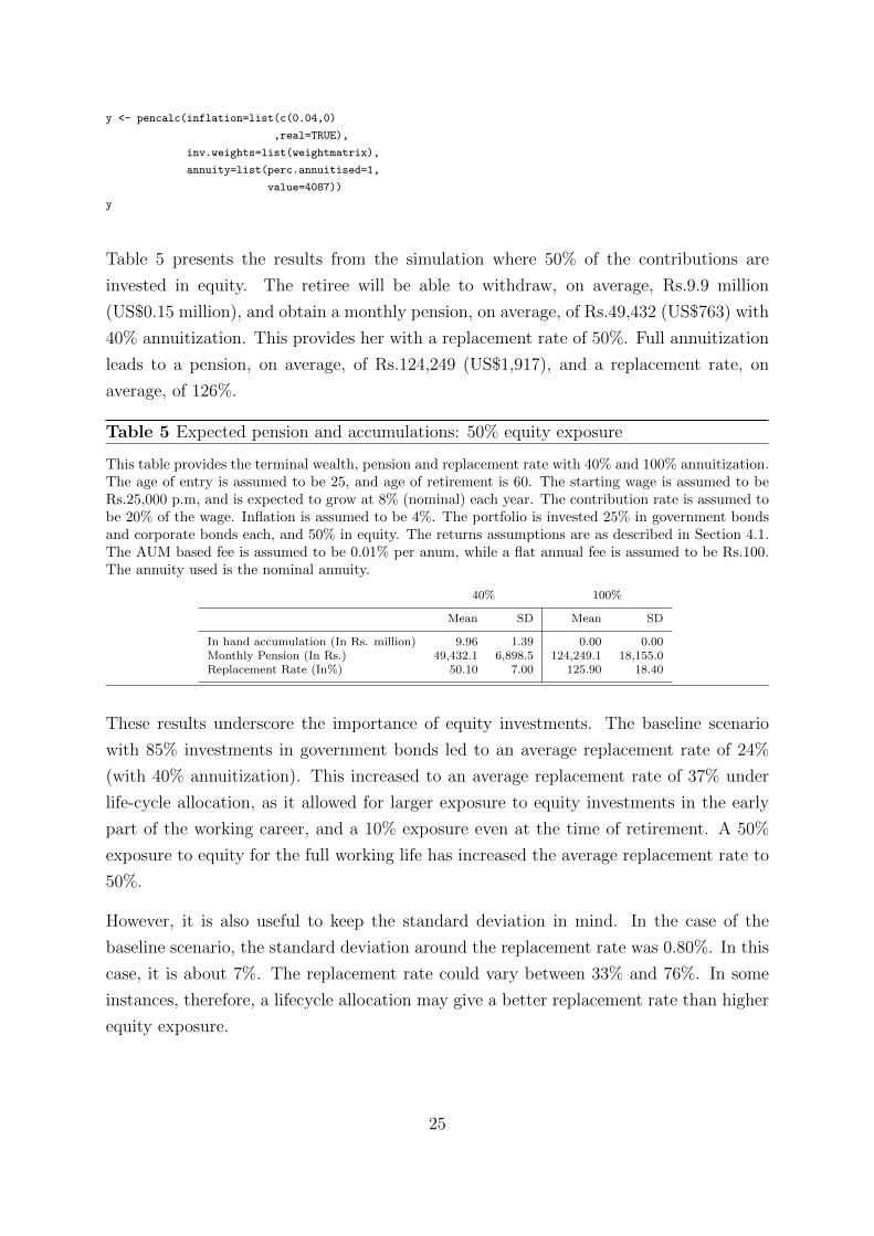
Table 5 presents the results from the simulation where 50% of the contributions are

invested in equity. The retiree will be able to withdraw, on average, Rs.9.9 million

(US$0.15 million), and obtain a monthly pension, on average, of Rs.49,432 (US$763) with

40% annuitization. This provides her with a replacement rate of 50%. Full annuitization

leads to a pension, on average, of Rs.124,249 (US$1,917), and a replacement rate, on

average, of 126%.

Table 5 Expected pension and accumulations: 50% equity exposure

This table provides the terminal wealth, pension and replacement rate with 40% and 100% annuitization.The age of entry is assumed to be 25, and age of retirement is 60. The starting wage is assumed to beRs.25,000 p.m, and is expected to grow at 8% (nominal) each year. The contribution rate is assumed tobe 20% of the wage. Inflation is assumed to be 4%. The portfolio is invested 25% in government bondsand corporate bonds each, and 50% in equity. The returns assumptions are as described in Section 4.1.The AUM based fee is assumed to be 0.01% per anum, while a flat annual fee is assumed to be Rs.100.The annuity used is the nominal annuity.

40% 100%

Mean SD Mean SD

In hand accumulation (In Rs. million) 9.96 1.39 0.00 0.00Monthly Pension (In Rs.) 49,432.1 6,898.5 124,249.1 18,155.0Replacement Rate (In%) 50.10 7.00 125.90 18.40

These results underscore the importance of equity investments. The baseline scenario

with 85% investments in government bonds led to an average replacement rate of 24%

(with 40% annuitization). This increased to an average replacement rate of 37% under

life-cycle allocation, as it allowed for larger exposure to equity investments in the early

part of the working career, and a 10% exposure even at the time of retirement. A 50%

exposure to equity for the full working life has increased the average replacement rate to

50%.

However, it is also useful to keep the standard deviation in mind. In the case of the

baseline scenario, the standard deviation around the replacement rate was 0.80%. In this

case, it is about 7%. The replacement rate could vary between 33% and 76%. In some

instances, therefore, a lifecycle allocation may give a better replacement rate than higher

equity exposure.

25

6.3.2 Lower equity returns

The current simulations have assumed an equity rate of return of 16%. This translates

to an equity premium of almost 9%. As more and more people participate in equity

markets, it is likely that the equity premium will go down. We, therefore, conduct the

same simulation with two different assumptions on equities:

1. We assume a 12% rate of return and a 20% standard deviation. This amounts to

an equity premium of 5%.

2. We assume a 10% rate of return and a 18% standard deviation. This amounts to

an equity premium of 3%.

The results are presented in Table 6. Column (1) shows the results with a 12% rate of

return, while Column (2) presents the results with a 10% rate of return.

Table 6 Expected pension and accumulations: Lower equity premium (40% annuitiza-tion)

This table provides the terminal wealth, pension and replacement rate for a 12% and 10% equity return.Assumptions on government and corporate bonds are the same as in Section 4.1. The age of entry isassumed to be 25, and age of retirement is 60. The starting wage is assumed to be Rs.25,000 p.m, andis expected to grow at 8% (nominal) each year. The contribution rate is assumed to be 20% of thewage. Inflation is assumed to be 4%. The portfolio is invested according to the life-cycle allocation. TheAUM based fee is assumed to be 0.01% per anum, while a flat annual fee is assumed to be Rs.100. Theannuitization rate is assumed to be 40%. The annuity used is the nominal annuity.

12% return 10% return

Mean SD Mean SD

In hand accumulation (In Rs. million) 6.64 0.68 5.51 0.49Monthly Pension (In Rs.) 32,952.0 3,398.3 27,321.2 2,429.1Replacement Rate (In%) 33.40 3.40 27.70 2.50

As seen in Column (1), the average pension is now Rs.33,000 (US$509), the average

terminal value is Rs.6.6 million (US$0.1 million) and the average replacement rate is

33%. The standard deviation is at 3.4%. Thus, as equity markets mature, we will see

a lowering of the equity premium, and a consequent lowering of the replacement rates

from greater equity exposure. If equity returns fall to 10%, then the impact on outcomes

is even larger. The pension drops to Rs.27,370 (US$422), the average terminal value to

Rs.5.5 million (US$0.08 million), and the replacement rate to 28%.

26

6.4 Different annuity prices

We evaluate how the replacement rate varies with annuity prices. Ideally there would be

a clearly defined grid of all the annuity factors for individual and joint life annuities, by

gender for different ages and for differential ages between spouses. This is not available

for India - and hence in this iteration of the model the annuity pricing is more basic than

it will be in future versions.16

Table 7 presents the results from a simulation where the baseline assumptions remain

the same, except for annuity prices. As discussed in Section 4.2 we use the prices for

a nominal annuity (Column 1), for an annuity that provides 50% of the pension to the

surviving spouse (Column 2), and for an annuity that provides 100% of the pension to the

surviving spouse and return of purchase price to the next survivor (Column 3). We also

present results from an annuity price of Rs.6,667 (US$103) based on more conservative

assumptions (Column 4). The R-code is shown below.

library(penCalc)

set.seed(111)

x <- pencalc(inflation=list(c(0.04,0)

,real=TRUE))

x

set.seed(111)

y <- pencalc(inflation=list(c(0.04,0)

,real=TRUE),

annuity=list(perc.annuitised=0.4,

value=4400))

y

set.seed(111)

z <- pencalc(inflation=list(c(0.04,0)

,real=TRUE),

annuity=list(perc.annuitised=0.4,

value=5589))

z

set.seed(111)

a <- pencalc(inflation=list(c(0.04,0)

,real=TRUE),

annuity=list(perc.annuitised=0.4,

value=6667))

a

Table 7 presents the average monthly pension and replacement rate for the different

16To see an example of the grid of annuity factors that would be ideal see Sweden’s annual report on theirpension system and in particular the outcomes from the ’second pillar’ mandatory defined contributioncomponent.

27

Table 7 Expected pension and accumulations: different annuity types (40% annuitiza-tion)

This table provides the pension and replacement rate with 40% annuitization for five different annuitytypes. These include the nominal annuity (Column 1), annuity that provides 50% of the pension to thesurviving spouse (Column 2), annuity that provides 100% of the pension to the surviving spouse andreturn of purchase price to the next survivor (Column 3), hypothetical annuity prices of Rs.3000 (Column4) and Rs.6667 (Column 5). The age of entry is assumed to be 25, and age of retirement is 60. Thestarting wage is assumed to be Rs.25,000 p.m, and is expected to grow at 5% each year. The contributionrate is assumed to be 20% of the wage. Default life-cycle weights for allocation of contributions towardsthe three asset classes are used. The returns assumptions are 7% (nominal) for government bonds, 10%(nominal) for corporate bonds, and 16% (nominal) for equity, with a standard deviation of 25%. TheAUM based fee is assumed to be 0.01% p.a., while a flat annual fee is assumed to be Rs.100. The annuityused is the nominal annuity. All values are in nominal Rs.

Nominal 50 % spouse 100 % spouse WB price

In hand accumulation (In Rs. million) 7.41 7.41 7.41 7.41Accumulation std. dev (0.75) (0.75) (0.75) (0.75)Monthly Pension (In Rs.) 36,744.3 34,130.4 26,869.5 22,524.9Pension SD (3702.4) (3439.1) (2,707.4) (2269.7)Replacement Rate (In %) 37.2 34.6 27.2 22.8RR SD (3.8) (3.5) (2.7) (2.3)

annuity types. We find that as we move from a nominal annuity to an annuity that

provides 50% and 100% of the pension to the surviving spouse17, the average replacement

rate falls from 37% to 35% and 27% respectively (on 40% annuitization). This is not

surprising as the annuity price now has to factor in not only the life expectancy of the

subscriber, but also of the surviving spouse, thereby increasing its exposure to longevity

risk. It is a useful reminder that there is a trade-off between increasing benefits to

survivors and the replacement rate.

The last column shows the pension and replacement rate for a price of Rs.6,667. This

corresponds to an annuity factor of 18, which is close to the annuity factor calculated

by the World Bank for a female retiring at age 65 in 2040.18 The average replacement

rate further falls to 23%. Given improvements in mortality, it is very likely that annuity

prices will rise considerably, resulting in lower replacement rates. We would suggest that

policy makers be cautious in the use of annuity prices, and conduct greater sensitivity

analysis given that such prices are usually national averages which overstate mortality for

civil servants, and understate them for the informal poor. This should also raise serious

questions on how to design the payout phase for the NPS.19

17This option also provides for the return of purchase price to survivors on the death of the survivingspouse.

18This number has been sourced from World Bank, Presentation to Pay and Pension Committee, 2015.19See Sane (2016) for a discussion on policy questions on the design of the draw down phase of the NPS.

28

6.5 Varying contribution rates

In the case of informal sector workers, a constant contribution rate may not be feasible.

This can be handled by using a vector of wages, and a contribution rate of 100%. This

effectively makes the values entered in the wage the actual contribution.

In the example described below, we simulate 36 values for wage from a normal distribution

with a mean of Rs.3,000 (US$46) and a standard deviation of Rs.100 (US$1.5). The

generated wage profile is presented in the appendix. We then use a contribution rate

of 100%. All the other assumptions remain the same as that of the life-cycle portfolio

allocation example described in Section 6.2. The R-code is shown below.

library(penCalc)

wage = round(rnorm(36, 3000, 100),0)

set.seed(111)

x <- pencalc(wage=list(wage

,0

,1

,initial.amount=0),

inflation=list(c(0.04,0)

,real=TRUE))

x

#100 %

set.seed(111)

y <- pencalc(wage=list(wage

,0

,1

,initial.amount=0),

inflation=list(c(0.04,0)

,real=TRUE),

annuity=list(perc.annuitised=1,

value=4087))

y

Table 8 presents the results from the simulation. The replacement rate is meaningless in

this context, and hence is not reported in the table. The informal sector worker can hope

to get an average monthly pension of Rs.13,454 (US$208) with 40% annuitization, or an

average monthly pension of Rs.33,635 (US$519) with 100% annuitization.

29

Table 8 Expected pension and accumulations: Varying contribution rate

This table provides the terminal wealth, pension and replacement rate with 40% and 100% annuitization.The age of entry is assumed to be 25, and age of retirement is 60. The wages are drawn from a normaldistribution with a mean of Rs.3000 and a standard deviation of 100. The contribution rate is assumed tobe 100%. Inflation is assumed to be 4%. The simulation uses the default life-cycle weights for allocationof contributions towards the three asset classes. The returns assumptions are as described in Section 4.1.The AUM based fee is assumed to be 0.01% per anum, while a flat annual fee is assumed to be Rs.100.The annuity used is the nominal annuity.

40% 100%

Mean SD Mean SD

In hand accumulation (In Rs. million) 2.71 0.34 0.00 0.00Monthly Pension (In Rs.) 13,454.1 1,698.3 33,635.2 4,245.9

7 Conclusion and Future Work

This paper sets out initial results from a new modeling exercise using penCalc based

on an open source software language “R” that is popular in the academic and modeling

communities. The initial results are presented (and the model made freely available) to

illustrate the tool. It is simple to tailor to different countries and any user determined

scenarios. The tool is illustrated for India’s National Pension System (NPS) - and presents

a range of scenarios based on actual and forecast parameters.

Hence, the aim of the paper is not to present the perfect model for India - but to show

how the tool works so policy makers and regulators can see its potential advantages

and develop it for their own uses. There are many extensions that could be developed,

which will be the subject of future work. These include: the correlation matrices between

the different assets (although the model is focused on the terminal values for pensions

rather than aiming to illustrate the annual pathway); deeper sensitivity analysis on the

key variables; increasing the sophistication of the annuity pricing so that it can include

uncertainty in relation to life expectancy and be driven from the stochastic outputs for

interest rates. This was not a feature of the initial work because annuity pricing is

unusual in India - partly given the nature of the annuity product which includes a return

of premium at death which reduces the variability of payouts with respect to different

life expectancy. Differential pricing to reflect difference in age between spouses will also

be added.20

The tool already allows policy makers and regulators to input different data and assump-

tions for the likely experience of different groups - for example different wage profiles to

20Extensions on annuities will also be able to draw on new work on payout options that may be moretailored to developing countries, including re-pricing or variable annuities that reduce the need forextensive mortality data and reduce the initial pricing risk see (Inglis and Price, 2017)

30

investigate different occupations or differences by gender or the impact of marital sta-

tus on labor market attachment - and then apply a tax “haircut” to terminal values

and income depending on their levels and hence tax bracket. However, at this stage

the user needs to find the right data and run the specific scenarios. Future work could

focus on simpler and more intuitive modeling to deliver multiple outputs for each group

simultaneously, and automate the tax calculation.

The modeling tool presented is placed in the international context by highlighting mod-

eling by regulators and pension funds in other jurisdictions. Some of these are more

complex or complete than the results in this paper - but by explaining the initial model

and making the coding freely available the authors hope to provide a powerful yet simple

and low cost tool that can be widely adopted and adapted.

31

Appendix

Package installation

The package may be installed as follows

devtools::install github("renukasane/penCalc").

Investment weights

Investment weights for the baseline function according to the lifecycle profile:

32

goi bonds corp bonds equity

25 0.10 0.25 0.65

26 0.10 0.25 0.65

27 0.10 0.25 0.65

28 0.10 0.25 0.65

29 0.10 0.25 0.65

30 0.10 0.25 0.65

31 0.10 0.25 0.65

32 0.10 0.25 0.65

33 0.10 0.25 0.65

34 0.10 0.25 0.65

35 0.10 0.25 0.65

36 0.13 0.24 0.63

37 0.16 0.24 0.61

38 0.18 0.23 0.58

39 0.21 0.23 0.56

40 0.24 0.22 0.54

41 0.27 0.21 0.52

42 0.30 0.21 0.50

43 0.32 0.20 0.47

44 0.35 0.20 0.45

45 0.38 0.19 0.43

46 0.41 0.18 0.41

47 0.44 0.18 0.39

48 0.46 0.17 0.36

49 0.49 0.17 0.34

50 0.52 0.16 0.32

51 0.55 0.15 0.30

52 0.58 0.15 0.28

53 0.60 0.14 0.25

54 0.63 0.14 0.23

55 0.66 0.13 0.21

56 0.69 0.12 0.19

57 0.72 0.12 0.17

58 0.74 0.11 0.14

59 0.77 0.11 0.12

60 0.80 0.10 0.10

33

Simulated wage profile for informal sector workers

wage

1 2797.002 3041.003 2924.004 3068.005 3073.006 2777.007 3165.008 3170.009 2892.00

10 2888.0011 2934.0012 2894.0013 2960.0014 2919.0015 3037.0016 2855.0017 2986.0018 3065.0019 2866.0020 2901.0021 2890.0022 2990.0023 3002.0024 3112.0025 3095.0026 2912.0027 3056.0028 3092.0029 3064.0030 2955.0031 3046.0032 3164.0033 3206.0034 2990.0035 2992.0036 2982.00

34

References

Antolin, P. (2009). “Private Pensions and the Financial Crisis: How to Ensure Adequate

Retirement Income from DC Pension Plans”. In: OECD Journal: Financial Market

Trends 2009.2.

Antolin, P. and O. Fuentes (2012). Communicating Pension Risk to DC Plan Members:

The Chilean Case of a Pension Risk Simulator. OECD Working Papers on Finance,

Insurance and Private Pensions, No. 28. OECD Publishing. doi: http://dx.doi.org/

10.1787/5k9181hxzmlr-en.

Antolin, P., S. Payet, and J. Yermo (2010). Assessing Default Investment Strategies in

Defined Contribution Pension Plans. OECD Working Papers on Finance, Insurance and

Private Pensions, No. 2. OECD Publishing. url: http://10.1787/5kmdbx1nhfnp-en.

Cannon, E. and I. Tonks (Jan. 2004). UK Annuity Rates and Pension Replacement Ratios

1957 - 2002. Centre for Research in Applied Macroeconomics. University of Bristol.

Dimson, E., P. Marsh, and M. Staunton (2017). Credit Suisse Global Investment Returns

Yearbook 2017. Credit Suisse, London.

Dowd, K. and D. Blake (Sept. 2013). Good Practice Principles in Modelling Defined

Contribution Pension Plans. Discussion Paper PI-1302. The Pensions Institute, Cass

Business School.

Hoyo, C., J. Alonso, and D. Tuesta (Jan. 2015). “A model for the pension system in Mex-

ico: diagnosis and recommendations”. In: Journal of Pension Economics and Finance

14.01. Cambridge University Press, pp. 76–112.

Inglis, E. and W. Price (2017). “Paying the Pension: Markets, Products and Choices”. In:

Protecting the Next Billion Against Old Age Poverty: Global Lessons for Local Action.

Ed. by Parul Seth Khanna, William Price, and Gautam Bhardwaj. Narosa Publishing

House, India.

Ionescu, L. and J. Yermo (2014). Stress Testing and Scenario Analysis of Pension Plans.

IOPS Working Papers on Effective Pensions Supervision, No. 19: International Orga-

nization of Pension Supervisors, Paris.

James, Estelle and Renuka Sane (2003). “Annuity markets in India: Do consumers get

their money’s worth?” In: Economic and Political Weekly XXXVIII.8.

Nair, Remya and Aparna Iyer (Aug. 2016). Govt notifies inflation target of 4%, in line

with RBI. liveMint. https://goo.gl/ZATwDd.

Pandey, I. M. (2015). Financial Management. Eleventh edition. ISBN: 978-93259-8229-1.

Vikas Publishing House Private Limited.

Parekh, Deepak (2009). Investment regulations for the New Pension System for the in-

formal sector. Tech. rep. PFRDA.

35

Price, W., J. Ashcroft, and M. Hafeman (2016). Outcome Based Assessments for Private

Pensions: A Handbook. Washington DC: World Bank Group.

pwc (2013). Global wage projections to 2030. Report. https://www.pwc.co.uk/assets/pdf/global-

wage-projections-sept2013.pdf: PricewaterhouseCoopers.

Sane, Renuka (Dec. 2016). Designing the payout phase of the National Pension System.

Ajay Shah’s blog. https://goo.gl/tLtE3y.

Sane, Renuka and Susan Thomas (2014). The way forward for India’s National Pension

System. Working Paper WP-2014-022. IGIDR.

Shah, Ajay (May 2015). Understanding the Indian financial environment. Ajay Shah’s

blog. https://goo.gl/5zV0Pp.

Stanko, D. (Dec. 2015). The concept of Target Retirement Income: supervisory challenges.

IOPS Working Papers on Effective Pensions Supervision, No.25.

Stewart, Fiona (2014). Proving incentives for long-term investment by pension funds:

the use of outcome-based benchmarks. Policy Research Working Paper No. WPS 6885.

Washington, DC: World Bank Group.

36