1

Simplifying general equilibrium analysis through a

modular structure: MAGNET

Paper for the 16th Annual Conference on Global Economic Analysis " New

Challenges for Global Trade in a Rapidly Changing World", June 12 -14 2013,

Shanghai, China

Geert Woltjer, (LEI Wageningen UR)

Abstract

This paper discusses some philosophy behind the MAGNET modelling system.

One basic idea is that the model code and the code to manipulate data is split in

more or less independent components. A second basic idea is that the

manipulation of data and scenarios should be coded completely. A system called

DSS has been developed to guide data manipulations, model aggregation and

simulations in a systematic way, and to store all choices for model code used,

data used and shocks given in the simulations in a standard manner. This

enables to reuse procedures that have been developed and to reproduce

principles of simulation when the GTAP database or other databases change, or

when the regional or commodity aggregation changes. A system called

GEMSE_Analist helps in interaction with the DSS system to analyse scenario

results in a systematic manner. An interface for coding called GTREE allows also

for reusing the same code with different sets, parameters or variables at

different places as a type of subroutine. Finally, the structuring of code through

GTREE helps to make the code more intuitive if the philosophy of intuitive coding

is followed. In summary, a number of important issues that are relevant to work

with the modular approach of MAGNET are discussed.

Corresponding author: Geert Woltjer.

Email address: Geert.Woltjer@wur.nl , Tel.: +31 70 3358382

2

Contents

Introduction ............................................................................................................................................. 2

The ingredients of the modular approach .............................................................................................. 4

GTREE .................................................................................................................................................. 4

Regional sets ........................................................................................................................................ 5

Versioning system and splitting model code in files ........................................................................... 6

Scenarios and DSS ............................................................................................................................... 6

Analysing results:the GEMSE_Analist .................................................................................................. 8

DSS for model settings, model aggregation and database manipulations ......................................... 9

Conclusion ......................................................................................................................................... 10

GTREE to prevent repetition of code .................................................................................................... 10

Creating different versions of model and data ..................................................................................... 12

The crucial importance of documentation ............................................................................................ 13

Intuitive programming strategies .......................................................................................................... 13

Conclusion ............................................................................................................................................. 15

References ............................................................................................................................................. 15

Introduction

How to feed the growing world populations and fulfil and reduce climate change

impact at the same time is one of the key challenges in the world. This enormous

challenge implies an increasing complexity and interconnectivity of for example

the agricultural, land and energy using sectors and disciplines. The issues

become so complex that modelling teams have to work together to contribute to

this challenge.

The philosophy of MAGNET (Modular Applied GeNeral Equilibrium Tool) is in line

with the GTAP philosophy to lower entry barriers for CGE analyses and it aims to

facilitate working in (cross-institutional) modelling teams for more complex

models. MAGNET is a modular global CGE model that covers the whole economy

and has been used extensively in agricultural, environmental and trade policy

3

analysis. MAGNET builds on the global general equilibrium Global Trade Analysis

Project (GTAP) model and is the successor of LEITAP (Meijl, et al. 2006, Banse et

al. 2008). MAGNET adopts a modular approach, whereby the standard GTAP-

based core can be augmented with modules depending on the purpose of the

study. Therefore MAGNET contains some institutional innovations and is

supported by various tools like a tool that structures the code (GTREE), a tool to

automatize, structure and document data procedures (DSS), a tool to run and

analyse scenarios (another module of DSS and GEMSE_Analist) and a strategy to

structure mappings, separating modules, and administrating changes. MAGNET

supports more users, more developers, larger flexibility, greater reliability and

more attractive tools. Currently the system is used at LEI-WUR, JRC-IPTS and

vTI. While the basic principles of the MAGNET system were discussed in a special

session of the GTAP conference 2012, during the last year the system has been

refined and a version 2 release has been made for distribution to the direct

partners.

This paper discusses the philosophy behind MAGNET including a number of

innovations that are still under development. The basic issue is that making a

reliable and flexible modelling system that can be developed further by more

people requires a subtle interplay of a large number of tools and behavioural

rules. We will discuss first the mix of rules and tools, and then go into some

innovations. The first innovation is the development of our model code interface

GTREE to allow for a type of subroutines. The second is a more the development

of a system that allows to keep all model and data versions into one system

while at the same time allowing for selecting which parts you would like to have

in the system. The third issue is something we did find out from experience:

flexibility has its price in the sense that it allows to do also a lot of stupid things.

Good documentation and the development of standards helps to prevent the

biggest mistakes. Finally, good modelling and model use requires that the user

understands what he is doing. In many cases model code is not easy to read.

The modular approach gives the possibility to structure code in a more lucid way,

but this requires also that the programmer does it. We use the standard GTAP

code as an example how a modular organisation of code may increase lucidity of

the code.

4

The ingredients of the modular approach

The approach in MAGNET has a number of ingredients that are interdependent:

GTREE, component selection through regional sets, a simulation interface called

DSS, a tool for scenario analysis called GEMSE_Analalist, a structure managed by

other components of DSS to aggregate data and select model components and

structures within these components, and a structure to process external data and

GTAP data starting from the aggregation in which the data are supplied and

handled systematically through program code towards a detailed aggregation

that is used as the database for a large number of analyses in MAGNET. An

important component is also the svn versioning system in combination with

splitting program code in separate files through GTREE, that allows to track

changes. Especially the splitting of the code in small components prevents many

conflicts that may arise if a lot of people and institutions work on the same

model. Below we discuss some of these elements with the purpose of showing

how all elements are interrelated. For more complete descriptions of the

implementation we refer to Woltjer and Kuipers et al (2013) and Woltjer, Rutten

and Kuipers, 2013.

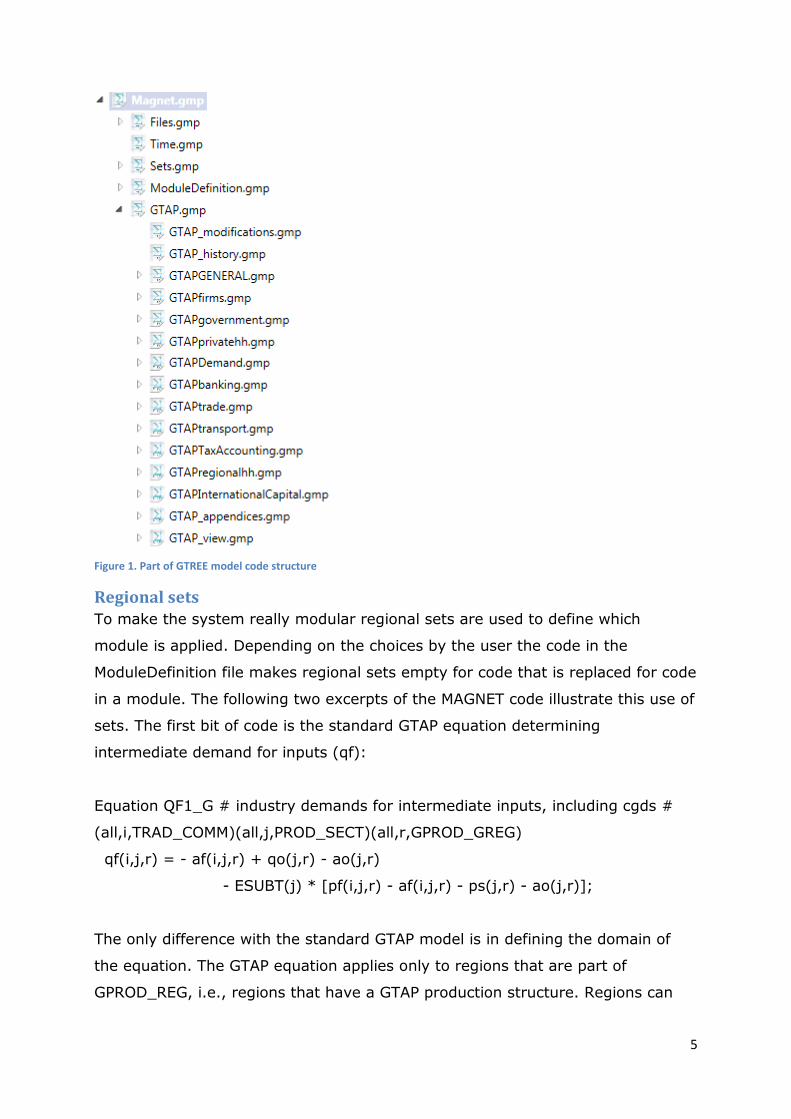
GTREE The first component is GTREE, a program that shows the structure of the

program code in components in a tree structure. GTREE structures code by

putting it in separate files (with extension gmp from Gempack). GTREE glues

these separate files together into one GEMPACK file in order to compile

everything further in the normal way. Figure 1 shows that MAGNET is the model,

and then there is a file where files are defined, a file where the Time variable is

defined, and a file where general GTAP sets are defined. The last module before

the real GTAP code is the file ModuleDefinition, that includes one file for each

module where the choice of module is defined.

5

Figure 1. Part of GTREE model code structure

Regional sets To make the system really modular regional sets are used to define which

module is applied. Depending on the choices by the user the code in the

ModuleDefinition file makes regional sets empty for code that is replaced for code

in a module. The following two excerpts of the MAGNET code illustrate this use of

sets. The first bit of code is the standard GTAP equation determining

intermediate demand for inputs (qf):

Equation QF1_G # industry demands for intermediate inputs, including cgds #

(all,i,TRAD_COMM)(all,j,PROD_SECT)(all,r,GPROD_GREG)

qf(i,j,r) = - af(i,j,r) + qo(j,r) - ao(j,r)

- ESUBT(j) * [pf(i,j,r) - af(i,j,r) - ps(j,r) - ao(j,r)];

The only difference with the standard GTAP model is in defining the domain of

the equation. The GTAP equation applies only to regions that are part of

GPROD_REG, i.e., regions that have a GTAP production structure. Regions can

6

also have a more elaborate and flexible CES production structure if they belong

to the set CETPROD_REG; then the same variable qf is governed by the following

equation:

Equation QF1_INP1_S1 # demands for inputs (HT 34) #

(all,i,INP1_S1)(all,j,SECTORS_S1)(all,r,CETPROD_REG)

qf(i,j,r)

= 0*time+ if(CS_INP1_S1(i,j,r)>0,

- af(i,j,r) + sum{k,SUB1_S1,qf(k,j,r)}

- sum{k,SUB1_S1,EL_PROD(k,j,r)}

* [pf(i,j,r) - af(i,j,r) - sum{k,SUB1_S1,pf(k,j,r)}]);

By using sets we can have different equations for the same variable co-existing

in the model. GEMPACK allows empty sets in which case the equations are

effectively removed from the model. Therefore, if no regions are assigned to

CETPROD_REG the equation above does not apply to any region and the model

has a standard GTAP specification.

Versioning system and splitting model code in files

The GTAP code (of which a small part is already in the file Files.gmp and

Sets.gmp) is split into a number of files. A small file called GTAPGeneral is

followed with the different components of the model, that are normally split

again in smaller components.

Although GTREE allows to structure code within a file, the splitting of code over

files is very important for simultaneous model development. Through the svn

versioning system the model code is stored in a central repository and model

developers can commit the code to a central repository. If people would be

working in the same file, inconsistencies in the common repository arise almost

always. By splitting the code in modules over different files and even splitting

code within modules over different files, different developers can work on

different modules without risking conflicts. Only if people work on the same part

of the code a careful coordination is required.

Scenarios and DSS Even if the code is organized well, running a large number of scenarios requires a

clear structuring of information. For this reason an interface is developed, called

7

Dynamic Steering System (DSS), that guides the user through a number of

implicit questions to which the answers are stored in so-called answer files. The

answer files in combination with the files that are stored in the database gives a

complete documentation of the scenario that the user runs. Archiving these

answer files in combination with the files that are used is essential for

documentation of simulation results, and gives also the opportunity to repeat the

same type of experiments with different databases.

Figure 2. A part of the DSS interface

A small part of the DSS interface is shown in figure 2. Each scenario has a name,

in this case the baseline for a simulation with a focus on India where Indian

development is calibrated on a GDP growth rate of 8% per year, called

BaseIndia8. The periods for simulation are defined, and below each period the

different elements for the simulation can be selected. The program sets files, the

parameter file, but also a file that contains the choices on which modules will be

used (model parameters file). Everything is stored in small files, that are in most

cases standardized. For example, the shock files consist of three files as

presented in figure 3.

8

Figure 3 Shock files selected for the simulation

The main role of DSS is to combine all the information given by the user into

command files and batch files that are used to run the scenario. The resulting

files remain available for the user, so the procedure is not a black box for the

user.

Analysing results:the GEMSE_Analist

Intimately related with DSS is the GEMSE_Analist. DSS stores all files generated

by GEMPACK in a subdirectory for solution files and a subdirectory for updated

files, and GEMSE_Analist recognizes these files as scenarios. The files have

standard names, including a combination of the scenario name and a reference

to the period. The strong point of the GEMSE_Analist is that it is able to read

variable definitions that can be applied to all scenarios, and that it is able to

aggregate regions and commodities to all user defined levels in a consistent

manner. This allows for fast analysis.

Figure 4 The GEMSE_Analist

Figure 4 shows part of the interface to present data in the GEMSE_Analist. At the

top left all scenarios are listed, with below it the opportunity to show results

relative to a reference scenario. To the right of this the periods are listed,

including a user defined one for the whole simulation period. To the right of this

9

you see that you can show the data as percentage changes, but also the

absolute numbers, yearly percentage changes or absolute changes, or the values

per capita or per unit of GDP. To the right of this box you see the list of variables

you can select (and that the user can change), followed by boxes to select

regions and products (in case of trade you need two regional dimensions, in case

of inputs you need two product dimensions). You see that the user has defined

regions for the specific analysis at hand: an aggregate world region, the EU27,

India, and the rest of the world, i.e. non-EUIndia. In the same manner the user

has defined the aggregates AGRI_CROPS and AGRI_Livestock, but also shows

the original GTAP livestock commodities. The results are shown in the table at

the bottom, that can also be shown as graphs or maps.

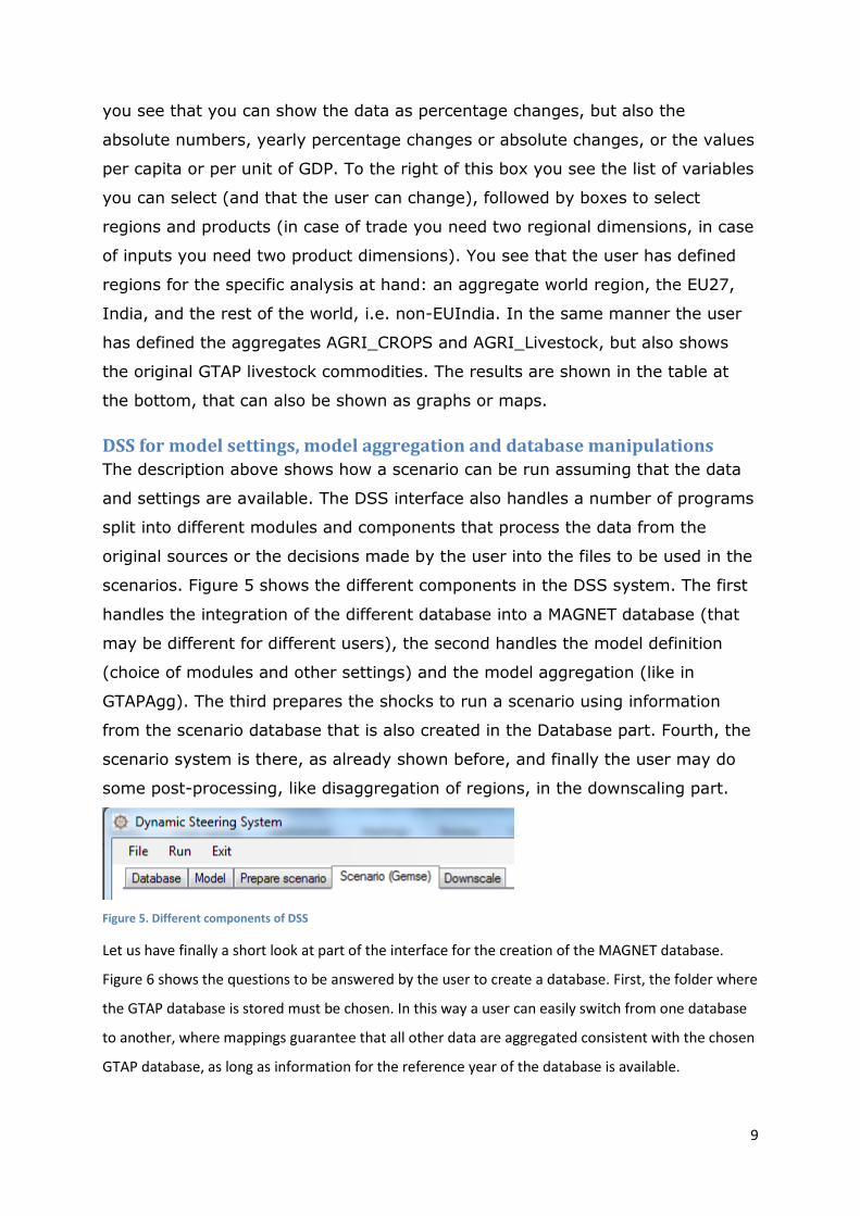
DSS for model settings, model aggregation and database manipulations The description above shows how a scenario can be run assuming that the data

and settings are available. The DSS interface also handles a number of programs

split into different modules and components that process the data from the

original sources or the decisions made by the user into the files to be used in the

scenarios. Figure 5 shows the different components in the DSS system. The first

handles the integration of the different database into a MAGNET database (that

may be different for different users), the second handles the model definition

(choice of modules and other settings) and the model aggregation (like in

GTAPAgg). The third prepares the shocks to run a scenario using information

from the scenario database that is also created in the Database part. Fourth, the

scenario system is there, as already shown before, and finally the user may do

some post-processing, like disaggregation of regions, in the downscaling part.

Figure 5. Different components of DSS

Let us have finally a short look at part of the interface for the creation of the MAGNET database.

Figure 6 shows the questions to be answered by the user to create a database. First, the folder where

the GTAP database is stored must be chosen. In this way a user can easily switch from one database

to another, where mappings guarantee that all other data are aggregated consistent with the chosen

GTAP database, as long as information for the reference year of the database is available.

10

Figure 6 Database tab of DSS

The second choice is the selection of files for other data, like those from FAO, WorldBank, and the

International Energy Agency. In a program developed by the user, called AddAndModifyData, the

data are aggregated or split through mainly automatic mappings towards the GTAP aggregation.

Which procedures to use is selected in the option “choose includes” where the modules to be used

can be selected. In this way the user can select a combination of standardly available routines, but

maybe also modules specifically developed for a project to manipulate the data. Also the GTAP data

can be manipulated through AddAndModifyData, using information from other data sources. Finally,

the user can add sectors, commodities, regions and endowments to the GTAP database, that

obviously must be filled with data using information from additional databases or some implicit

information in the GTAP database. For example, a fertilizer sector may be split from the chemical

sector assuming that all deliveries of the chemical sector to the crop sector are fertilizer deliveries, or

the fertilizer sector may be split using information on deliveries by other data sources like FAO.

Conclusion In summary, the MAGNET system is a very flexible system that tracks exactly all data processing from

original data and all model choices towards a database to be used in scenario’s. The model code is

developed in a modular manner allowing for multi-user development and easy selection of different

model and data choices by the user that is documented to a large extend automatically through the

DSS answer files and the SVN versioning system.

Although the discussion above is far from complete, below we discuss some special recent

developments in the MAGNET system.

GTREE to prevent repetition of code

One of the weaknesses of the GEMPACK language is that repetition of code can

only be accomplished by copying, and this generates risks of mistakes. This is

11

hard work, but the most important problem arises when you decide to change

this code. In that case you have to change this everywhere, with the risk of

making mistakes.

An example of code with a lot of repetition is a CES tree; it is just a repetition of

CES nests, but because different sets and equations are used, these must have

different names. A specific nest is the top nest, that has a zero profit condition

and therefore is a little bit difficult. In GTREE we see for the CES nest structure

two CES nest structures: Nest.gmp and Topnest.gmp (figure 7).

Figure 7 CES nest structure

Let us have a look a little bit more in detail in Nest.gmp, and as an example we

look at the equation for demand in subnest:

Equation QF1_INP@Y # demands for inputs of a subnest(HT 34) #

(all,i,INP@Y)(all,j,SECTORS)(all,r,CETPROD_REG)

qf(i,j,r)= - af(i,j,r) + sum{k,SUB@Y,qf(k,j,r)}

- sum{k,SUB@Y,EL_PROD(k,j,r)} * [pf(i,j,r) - af(i,j,r) - sum{k,@GSUB@Y,pf(k,j,r)}]);

A character to be replaced is refered to by an @, followed by the character. So,

@Y means that @Y is replaced. With which it is replaced is defined when the file

is included:

!$include Nest.gmp --Y=[8,7,6,5,4,3,2,1]!

Where –Y=[] tells that the file is copied 8 times, and that @Y is replaced by

respectively a 8, 7,...1. In this way the set of inputs INP@Y becomes in the

copies of the file respectively INP8, INP7.. INP1. Adding an extra subnest is very

easy. If you write:

!$include Nest.gmp --Y=[9,8,7,6,5,4,3,2,1]!

You will have a ninth subnest!

12

This implies that the GTREE system creates the possibility to write a complete

CES system with only one line for all the subnests.

The system is not only useful for the definition of CES trees or CET trees, but

also for example for a calibration procedure we use to calibrate the CDE

consumption function to price and income elasticities, or for the use of the same

procedure to add split different commodities from the GTAP database. The

system has even been used to duplicate all GTAP code in order to be able to run

some regions at a more detailed commodity level than the other regions in a

global model.

Creating different versions of model and data

The flexibility of the MAGNET system implies that a lot of data and modules are

available in the complete system for the user. But it may be that some data are

licensed and therefore are not allowed to be used by non-licensees, while for

users who like to use a simple system too much choices are available. For this

reason a set of batch files has been developed that copy the relevant information

to specific release directories that can be tailor made for the user. Although the

principle is simple, an easy way of selecting modules and data to be included

requires a careful structuring of the directories in the system. If you decide not

to include land use data, also all modules and data procedures that use these

data must not be included. By giving different consistent names related with

these procedures, this can be accomplished.

Another problem that arose using the system was that DSS adjusts a lot of files.

When a developer by accident commits a file to the repository he may overwrite

changes by others, creating a lot of problems. For this reason, all files that most

developers normally do not change, are also stored in separate subdirectories

and copied to the relevant places when the model directory is taken from the

repository. So, a number of files is stored in a separate directory and copied in

the right places before running the system, which also allows for having different

modules available for different user groups or different projects, while it helps

also to create custom made indicators for different projects.

In conclusion, the examples above are just examples to show how the reliability

and usefulness of a system like MAGNET depends on a large number of small but

important procedures.

13

The crucial importance of documentation

When other people started to use the flexible system developed by LEI, it

became obvious that user not acquainted with the background of the model may

use the system in an incorrect manner. For example, if you include a module on

the Common Agricultural Policy (CAP) of the EU with only a GTAP model, the

model will not generate plausible results. The effect of the CAP policies depends

fundamentally on the dynamics of the land and labour markets. For this reason,

modules that describe these dynamics must always be included when a CAP

module is run. So, a flexible system like in MAGNET requires careful

documentation, including reference to the intuition behind each module and the

relationship with other modules.

Although documentation is useful, also other features are important. The design

of the DSS system allows to develop standard answer files. These files work on

most aggregation, depending on how disciplined developers were in making the

code independent of aggregation. By supplying the standard answer files

(different answer files for different problems) inexperienced users have a starting

point for their simulations and only have to change these standards when they

have specific reasons for this. In this manner, the answer files of DSS are also a

type of documentation.

Intuitive programming strategies

Running a model requires that the user understands the model. Even a relatively

simple model like GTAP is in its standard form not always easy to understand. A

last issue discussed is the role of intuitive programming. In order to make code

easy to read, it is important that variable names are intuitive, that equation

names tell with which variables they are related, and that the ordering of the

code tells about the logic of the system. For this reason, for example the code of

the standard GTAP model has been reorganized into logical units where equation

names start with the name of the variable that is normally determined by the

equation.1

1 Variables names were already more or less logic in GTAP, and we have a strategy to start from the equations

of standard GTAP as it is to make entering the system easier for people who know standard GTAP.

14

Figure 8 GTAP private household

Let us describe an example. The way the GTAP code has been organized around

logical units has already been shown in figure 1. Figure 8 shows the contents of

one unit the private household. After consumption accounting and the definition

of the utility function parameters, total private demand and utility are

determined. Then income and price elasticities of demand are calculated, and in

the unit afterwards they are applied to determine private demand. This logic

already shows that private demand is simply calculated through the price and

income elasticities, and that calculation of the elasticities in a consistent manner

is done through a utility function. Finally, private demand is split over imported

and domestic demand using an Armington function.

If we dig deeper into the code for the last part, we see the following:

!Region Imported and domestic private demand (Armington)!

!Domestic demand of commodity i (qpd) grows with the total demand of

commodity i (qp) and grows more than total demand if the average price of

the commodity is based (pp) is higher than the domestic price (ppd), i.e.

when the domestic commodity is cheaper. Together with the equation for

import this is an Armington demand system that is basically a CES demand system

for applied for trade. The parameter ESUBD is the Armington substitution parameter, i.e.

When ESUBD is higher the effect of prices on imports is higher.!

Equation QPD1 !PHHLDDOM! # private consumption demand for domestic goods (HT 48) #

(all,i,TRAD_COMM)(all,r,GREG) qpd(i,r) = qp(i,r) + ESUBD(i) * [pp(i,r) - ppd(i,r)];

Equation QPM1 !PHHLDAGRIMP! # private consumption demand for aggregate imports (HT 49) #

(all,i,TRAD_COMM)(all,r,GREG) qpm(i,r) = qp(i,r) + ESUBD(i) * [pp(i,r) - ppm(i,r)];

15

First, we see that an explanation of code is provided. And then we see simply the

essential equations. The equations are named consistent with the variable

explained followed by a 1, and for people coming from GTAP the original GTAP

equation names are provided as a comment.

In summary, through structuring code and providing comments within the code

we try to make the code more intuitive for the users, and to make clear what is

really important (i.e. income and price elasticities determine consumption

demand).

Conclusion

The main message of this paper is that a good modelling system requires a balanced combination of

tools and behavioural rules. The way the code is structured into modules requires an interface to

make this lucid. The way scenarios are organized is related with the simulation interface DSS and the

tool to analyse data, GEMSE_analist. The complex system of creating model settings requires an

interface to create the required data and settings files, again through the DSS system. And a reliable

database requires well-documented and easy to handle procedures to process, aggregate and

disaggregate the data of different sources in a documented manner. And, finally, a good system

requires discipline in making the model code accessible and lucid for the reader.

References

Woltjer, Geert and Marijke Kuipers, et al (2013), The MAGNET model: Module

description, unpublished mimeo, LEI.

Woltjer, Geert, Martine Rutten and Marijke Kuipers (2013), Working with MAGNET: User

guide, unpublished mimeo, LEI.