seminar theorie komplexer systeme - heidelberg university · seminar theorie komplexer systeme •...

Seminar Theorie komplexer Systeme

Hidden Markov Models for biological systems

1

2

N…

1

2

N…

1

2

K…

…

…

…

1

2

N…

o1 o2 o3 oT

2

1

N

20

b

WS 2004/2005: 4-11-2004 Heermann - Universitat Heidelberg Seite 1


• We would like to identify stretches of sequences that are actually

functional (code for proteins or have regulatory functions) from

non-coding or junk sequences.

• In prokaryotic DNA we have only two kinds of regions, ignore

regulatory sequences which are coding (+) and non-coding (-) and

the four letters A,C,G,T.

A G

C T



• This simulates a very common phenomenon:

there is some underlying dynamic system running along

according to simple and uncertain dynamics, but we cannot

see it.

• All we can see are some noisy signals arising from the underlying

system. From those noisy observations we want to do things like

predict the most likely underlying system state, or the time history

of states, or the likelihood of the next observation



What are Hidden Markov Models good for?

• useful for modeling protein/DNA sequence patterns

• probabilistic state-transition diagrams

• Markov processes - independence from history

• hidden states



History

• voice compression, information theory

• speech = string of phonemes

• probability of what follows what

Rabiner, L.R. (1989). A tutorial on hidden Markov models and selected

applications in speech recognition. Proceedings of the IEEE, 77:257-286.



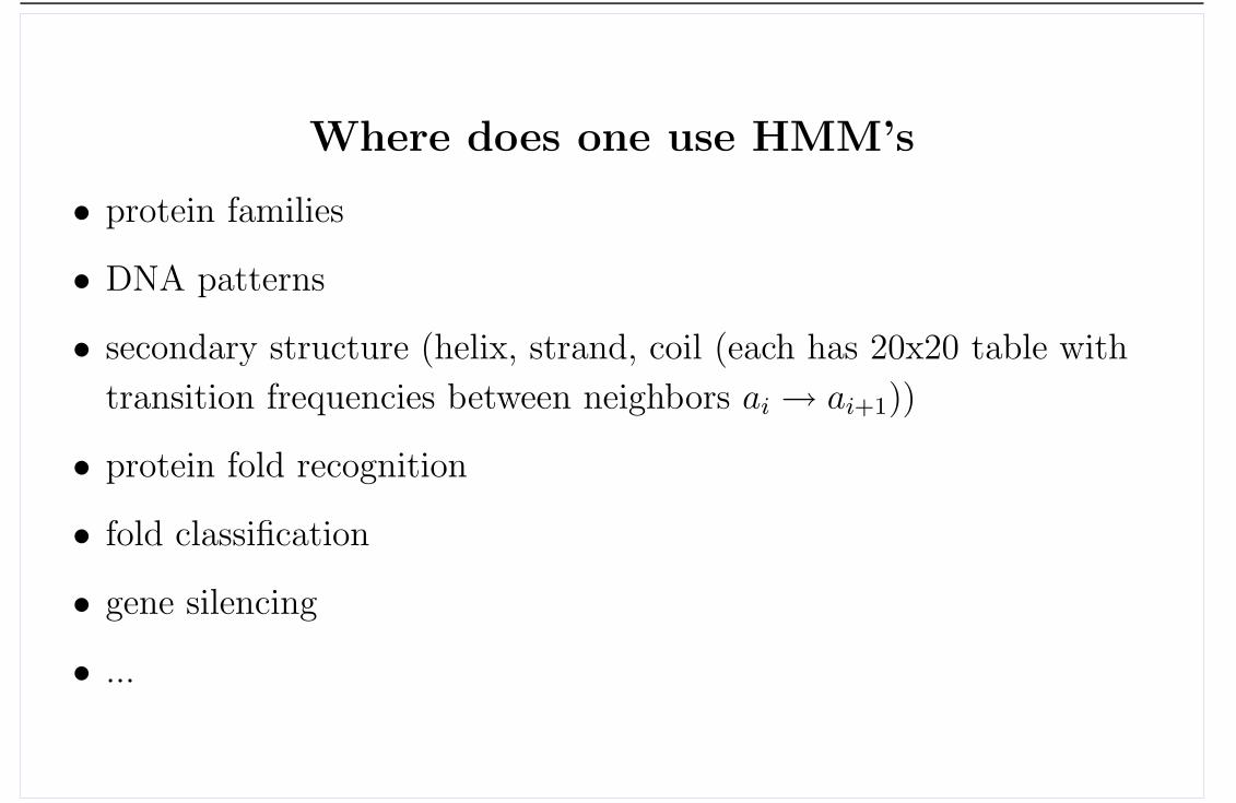
Where does one use HMM’s

• protein families

• DNA patterns

• secondary structure (helix, strand, coil (each has 20x20 table with

transition frequencies between neighbors ai → ai+1))

• protein fold recognition

• fold classification

• gene silencing

• ...



• Example: CpG Islands

– Regions labeled as CpG islands −→ + model

– Regions labeled as non-CpG islands −→ - model

– Maximum likelihood estimators for the transition probabilities for

each model

ast =cst∑t′ cst′

and analogously for the - model. cst is the number of times letter t

followed letter s in the labeled region



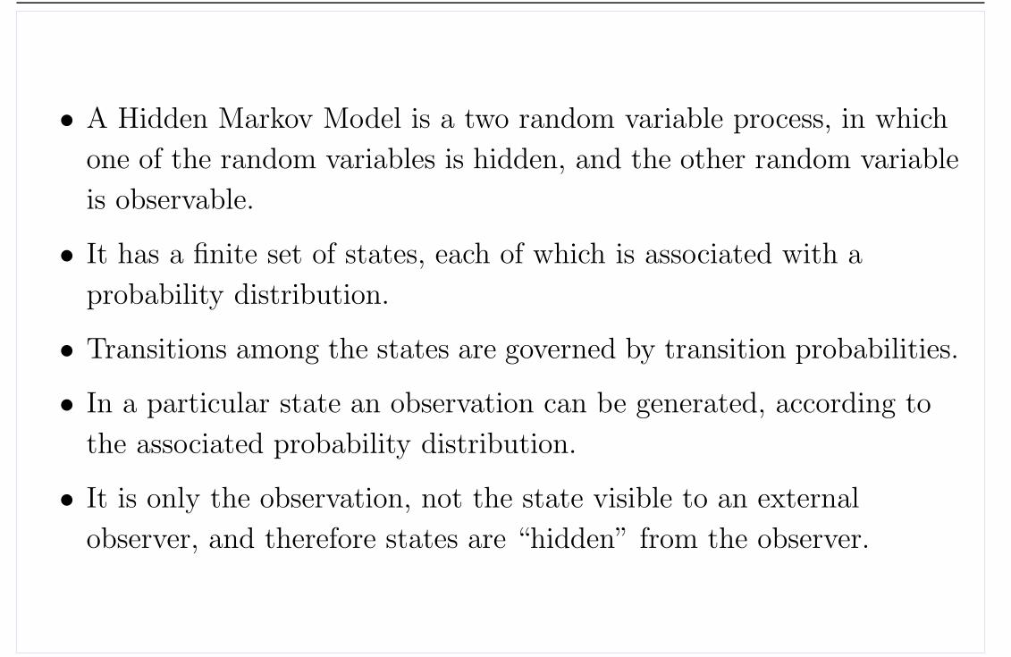
• A Hidden Markov Model is a two random variable process, in which

one of the random variables is hidden, and the other random variable

is observable.

• It has a finite set of states, each of which is associated with a

probability distribution.

• Transitions among the states are governed by transition probabilities.

• In a particular state an observation can be generated, according to

the associated probability distribution.

• It is only the observation, not the state visible to an external

observer, and therefore states are “hidden” from the observer.



• Example:

– For DNA, let + denote coding and - non-coding. Then a possible

observed sequence could be

O = AACCTTCCGCGCAATATAGGTAACCCCGG

and

Q = −−+ + + + + + + + + + + + + + + + +−−−−−−−−• Question: How can one find CpG - islands in a long chain of

nucleotides?

• Merge both models into one model with small transition

probabilities between the chains.



A Hidden Markov Model (HMM) λ =< Y, S,A,B >

consists of:

• an output alphabet Y = {1, ..., b}• a state space S = {1, ..., c} with a unique initial state s0

• a transition probability distribution A(s′|s)• an emission probability distribution B(y|s, s′)



• HMMs are equivalent to (weighted) finite state automata

with outputs on transitions

• Unlike MMs, constructing HMMs, estimating their

parameters and computing probabilities are not so

straightforward



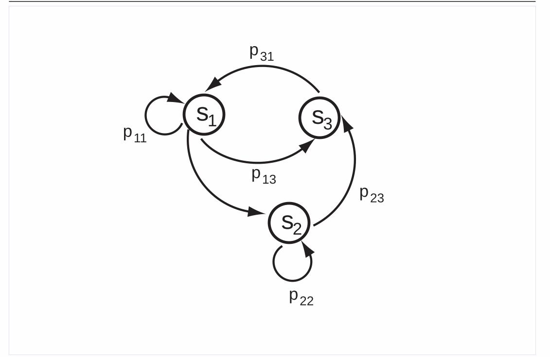
s1

s2

s3

p31

p11

p22

p13p23



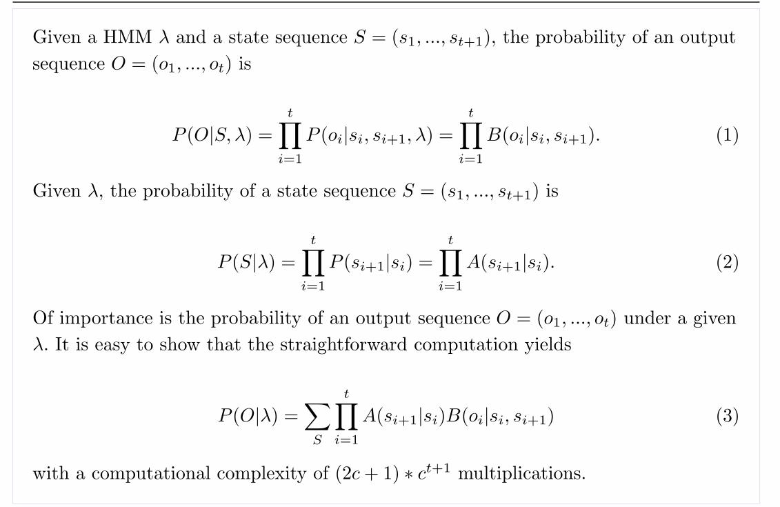
Given a HMM λ and a state sequence S = (s1, ..., st+1), the probability of an outputsequence O = (o1, ..., ot) is

P (O|S, λ) =t∏

i=1

P (oi|si, si+1, λ) =t∏

i=1

B(oi|si, si+1). (1)

Given λ, the probability of a state sequence S = (s1, ..., st+1) is

P (S|λ) =t∏

i=1

P (si+1|si) =t∏

i=1

A(si+1|si). (2)

Of importance is the probability of an output sequence O = (o1, ..., ot) under a givenλ. It is easy to show that the straightforward computation yields

P (O|λ) =∑

S

t∏

i=1

A(si+1|si)B(oi|si, si+1) (3)

with a computational complexity of (2c + 1) ∗ ct+1 multiplications.



• Multiple Sequence Alignments

– In theory, making an optimal alignment between two sequences iscomputationally straightforward (Smith-Waterman algorithm), but aligning alarge number of sequences using the same method is almost impossible (e.g.O(tN )).

– The problem increases exponentially with the number of sequences involved(the product of the sequence lengths).

– Statistical Methods:∗ Expectation Maximization Algorithm (deterministic)∗ Gibbs Sampler (stochastic)∗ Hidden Markov Models (stochastic)

– Advantages for HMM: theoretical explanation, no sequence ordering, noinsertion and deletion penalties, using prior information

– Disadvantage for HMM: large number of sequences for training



.8

.2

ACGT

ACGT

ACGT

ACGT

ACGT

ACGT.8

.8 .8.8

.2.2.2

.2

1

ACGT .2

.2

.2

.4

1. .4 1. 1.1.

.6.6

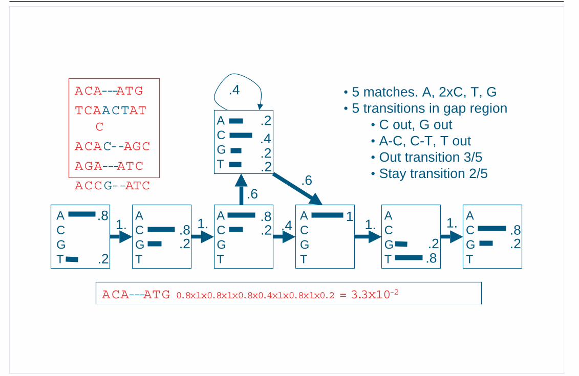
.4ACA---ATG

TCAACTATC

ACAC--AGC

AGA---ATC

ACCG--ATC

• 5 matches. A, 2xC, T, G• 5 transitions in gap region

• C out, G out• A-C, C-T, T out• Out transition 3/5• Stay transition 2/5

ACA---ATG 0.8x1x0.8x1x0.8x0.4x1x0.8x1x0.2 = 3.3x10-2



By Forward-backward, Viterbi, Baum-Welch (or EM) algorithms, (1) find Prob. ofthe observation sequence given the model; (2) find the most likely hidden statesequence given the model and observations; (3) adjust parameters to maximize theirProb. given observations.



• There are three basic problems:

1. Given a model, how likely is a specific sequence of

observed values (evaluation problem).

2. Given a model and a sequence of observations, what is

the most likely state sequence in the model that

produces the observations (decoding problem).

3. Given a model and a set of observations, how should

the model’s parameters be updated so that it has a

high probability of generating the observations

(learning problem).



Forward algorithm

• We define αs(i) as the probability being in state s at

position i:

αs(i) = P (o1, ..., oi, si = s|λ) (4)

• Base case: αs(1) if s = s0 and αs(0) = 0 otherwise

• Induction:

αs(i + 1) = maxs∈S

A(s|s′)B(oi|s′, s)αs(i) (5)

• Finally, at the end:

P (o1, ..., ok|λ) =∑

s∈S

αs(k) (6)



Forward algorithm

• Partial sums could as well be computed right to left

(backward algorithm), or from the middle out

• In general, for any position i:

P (O|λ) =∑

s∈S

αs(i)βs(i) (7)

• This algorithm could be used, e.g. to identify which λ is

most likely to have produced an output sequence O



What is the most probable path given observations

(decoding problem)?

• given o1, ..., ot what is

argmaxSP (s, o1, ...ot|λ)

• slow and stupid answer:

argmaxS

P (o1, ..., ot|s)P (s)

P (o1, ..., ot)



Viterbi algorithm

• We define δs(i) as the probability of the most likely path

leading to state s at position i:

δs(i) = maxs1,...,si−1

P (s1, ..., si−1, o1, ..., oi−1, si = s|M) (8)

• Base case: δs(1) if s = s0 and δs(0) = 0 otherwise



Viterbi algorithm

• Again we proceed recursively:

δs(i + 1) = maxs∈S

A(s|s′)B(oi|s′, s)δs(i) (9)

and since we want to know the identity of the best state

sequence and not just its probability, we also need

Ψ(i + 1) = argmaxs∈SA(s|s′)B(oi|s′, s)δs(i) (10)

• Finally, we can follow Ψ backwards from the most likely

final state



Viterbi algorithm

• The Viterbi algorithm efficiently searches through |S|Tpaths for the one with the highest probability in

O(T |S|2) time

• In practical applications, use log probabilities to avoid

underflow errors

• Can be easily modified to produce the n best paths

• A beam search can be used to prune the search space

further when |S| is very large (n-gram models)



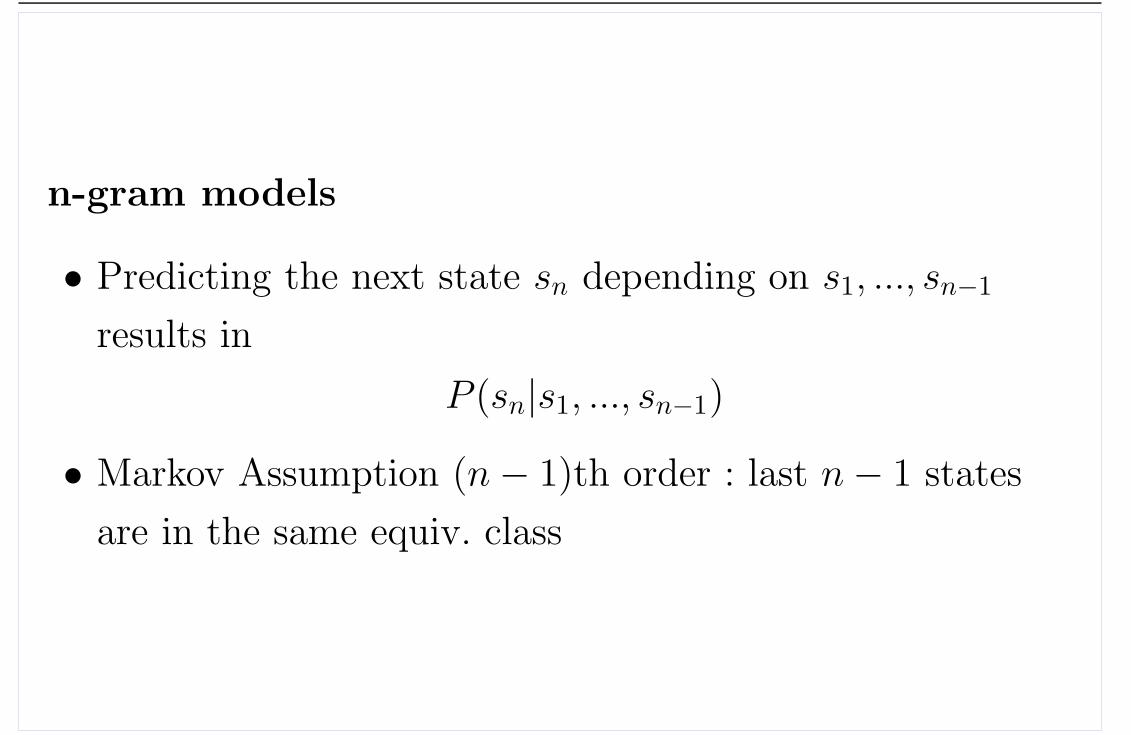
n-gram models

• Predicting the next state sn depending on s1, ..., sn−1

results in

P (sn|s1, ..., sn−1)

• Markov Assumption (n − 1)th order : last n − 1 states

are in the same equiv. class



Parameter estimation

• Given an HMM with a fixed architecture, how do we

estimate the probability distributions A and B?

• If we have labeled training data, this is not any harder

than estimating non-Hidden Markov Models (supervised

training):

A(s′|s) =C(s → s′)∑s′′ C(s → s′′)

(11)

B(o|s, s′) =C(s → s′, o)C(s → s′)

(12)



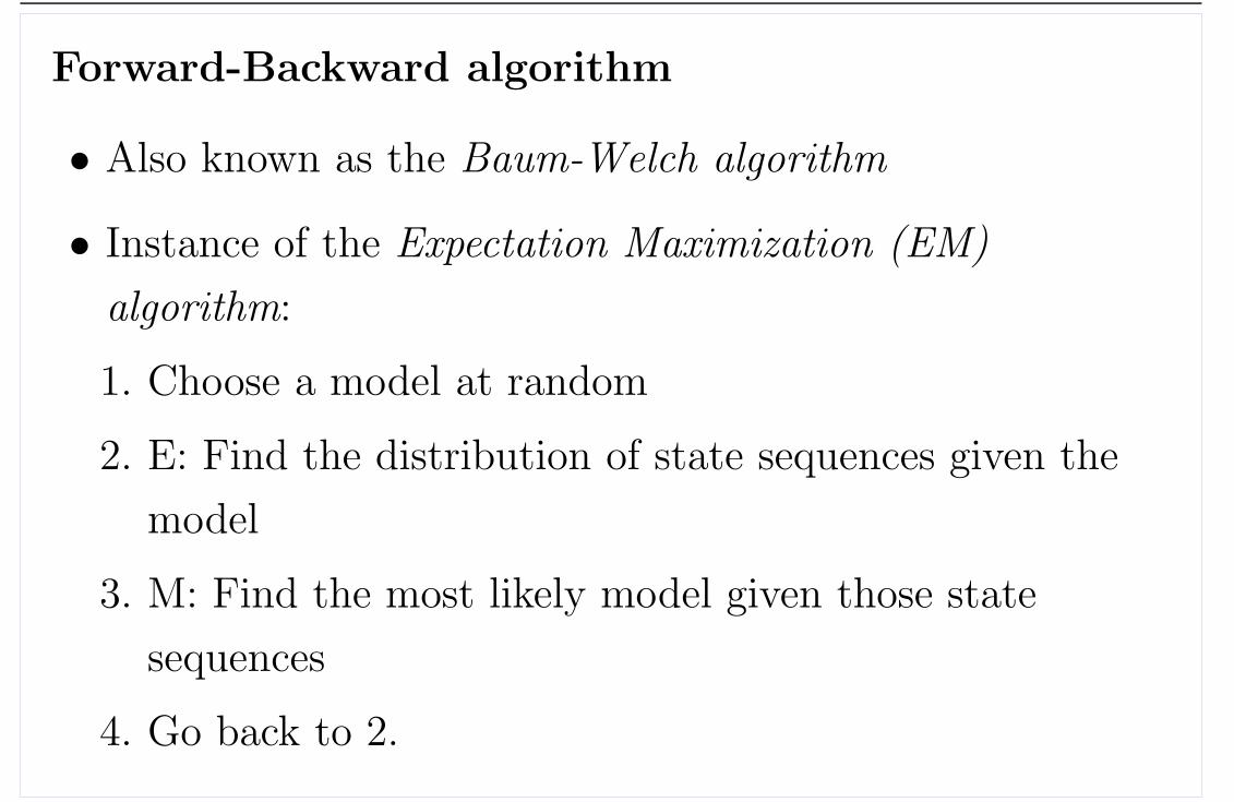
Forward-Backward algorithm

• Also known as the Baum-Welch algorithm

• Instance of the Expectation Maximization (EM)

algorithm:

1. Choose a model at random

2. E: Find the distribution of state sequences given the

model

3. M: Find the most likely model given those state

sequences

4. Go back to 2.




• Our estimate of A is:

A(s′|s) =E[C(s → s′)]E[C(s →?)]

(13)

• We estimate E[C(s → s′)] via τt(s, s′), the probability of moving from state s tostate s′ at position t given the output sequence O:

τt(s, s′) = P (st = s, st+1 = s′|O, λ) (14)

=P (st = s, st+1 = s′, O|λ)

P (O|λ)(15)

=αs(t)A(s|s′)B(ot+1|s, s′)βs′(t + 1)∑

s′′ αs′′(16)




• This lets us estimate A:

A(s′|s) =∑

t τt(s, s′)∑t

∑s′′ τt(s, s′′)

(17)

• We can estimate B along the same lines, using σt(o, s, s′), the probability ofemitting o while moving from state s to state s′ at position t given the outputsequence O

• Alternate re-estimating A from τ , then τ from A, until estimates stop changing

• If the initial guess is close to the right solution, this will converge to an optimalsolution



• A. Krogh, M. Brown, I. S. Mian, K. Sjander, and D. Haussler, Hidden Markovmodels in computational biology: Applications to protein modeling. Journal ofMolecular Biology, 235, 1501-1531 (1994)

• R. Durbin, S.R. Eddy, A. Krogh and G. Mitchison Biological sequence analysis,Cambridge University Press, 1998


seminar theorie komplexer systeme - heidelberg university · seminar theorie komplexer systeme •...

Documents