Supplementary Information

I. Methods: Ethics procedures, surveys, data collection software, & source code

This study was reviewed and approved by the Harvard University Institutional Review Board, approval #15-2529 and by the University of Vermont Institutional Review Board, approval #CHRMS-16-135. All study participants were informed of and acknowledged all study goals, expectations, and procedures, including data privacy procedures, prior to any data collection. Surveys were built using the Qualtrics survey platform. Analyses were conducted using the Python and R programming languages. Social media data collection apps were written in Python, using the Instagram developer’s Application Programming Interface (API). The survey for depressed participants collected age data from participants, and asked qualified participants questions related to their first depression diagnosis and social media usage at that time. These questions were given in addition to the CES-D scale. The purpose of these questions was to determine:

● The date of first depression diagnosis ● Whether or not the individual suspected being depressed before diagnosis, and, ● If so, the number of days prior to diagnosis that this suspicion began

In the case that participants could not recall exact dates, they were instructed to approximate the actual date. The survey for healthy participants collected age and gender data from participants. It also asked four questions regarding personal health history, which were used as inclusion criteria for this and three other studies. These questions were as follows:

● Have you ever been pregnant? ● Have you ever been clinically diagnosed with depression? ● Have you ever been clinically diagnosed with Post-Traumatic Stress Disorder? ● Have you ever been diagnosed with cancer?

Participants’ responses to these questions were not used at all in analysis, and only served to include qualified respondents in each of the various studies, including the depression-related study reported here.

II. Methods: Face Detection

We used an elementary face detection script, based on an open source demonstration (https://gist.github.com/dannguyen/cfa2fb49b28c82a1068f). The main adjustment we made from the open source demo was to run through the detection loop twice, using two differing scale factors. A single scale factor had difficulty finding both small and large faces. Parameters used: scale_factors = [1.05, 1.4], min_neighbors = 4, min_size = (20px,20px) Algorithm accuracy was assessed by manually coding a random sample of 400 photos (100 photos from each of combination of depressed/healthy, detected/undetected). Detection accuracy was roughly equal across groups: Face detection accuracy:

Depressed, No face detected: 77% accurate Healthy, No face detected: 79% accurate

Depressed, 1+ faces detected: 59% accurate Healthy, 1+ faces detected: 61% accurate

The mean difference in counted faces (detected faces minus actual faces), indicated that the algorithm slightly undercounted the number of faces in photos, for both depressed participants

as well as healthy participants . In bothμ − .015, σ .21)( = 0 = 1 − .215, σ .07)(μ = 0 = 2 groups, the algorithm undercounted by less than a single face, on average.

III. Methods: Statistical framework

Bayesian logistic regression A Bayesian framework avoids many of the inferential challenges of frequentist null hypothesis significance testing, including reliance on p-values and confidence intervals, both of which are subject to frequent misuse and misunderstanding (38-41). For comparison, results from frequentist logistic regression output are included below; both methods are largely in agreement. Logistic regression was conducted using the MCMClogit function from the R package MCMCpack (42). This function asserts a model of the following form :

With the inverse link function:

And a multivariate Normal prior on 𝛽:

We selected “uninformative” priors for all parameters in 𝛽, with While, .0001.b0 = 0 B0 = 0 generally it is preferable to specify Bayesian priors, in this setting our parameters of interest were entirely novel, and so were not informed by prior literature or previous testing. The MCMClogit() function employs a Metropolis algorithm to perform Markov Chain Monte Carlo (MCMC) simulations. The Instagram model simulation used two MCMC chains of 100,000 iterations with a burn-in of 10,000 and no thinning. The use of thinning for achieving higher-precision estimates from posterior samples is questionable when compared to simply running longer chains (43). While no best practice has been established for how long an unthinned chain should be, Christensen et al. (44) advised: “Unless there is severe autocorrelation, e.g., high correlation with, say [lag]=30, we don't believe that thinning is worthwhile”. In our MCMC chains, we observed low autocorrelation at a lag of 30, and so felt confident in foregoing thinning. For comparison, we also ran a 100,000-iteration chain, thinned to every 10th iteration, with a burn-in of 5,000. While autocorrelation was noticeably reduced at shorter lags, this chain yielded near-identical parameter estimates from the posterior. Recall that Bayesian regression coefficients are not assigned p-values or any other significance measures conventional in frequentist null-hypothesis significance testing (NHST). We have provided Highest Posterior Density Intervals (HPDIs) for the highest probability at which the interval excludes zero as a possible coefficient value. For example, if a 99% HPDI is reported, it

means that, based on averaged samples from the simulated joint posterior distribution, the coefficient in question has a 99% probability of being non-zero. References to variable “significance” in the Results section relate only to the probability that a variable’s parameter estimate is non-zero, eg. “Variable X was significant with 99% probability”. Bayes factors were used to assess model fit. Given two models parameterized by, MM a b parameter vectors , and data , the Bayes factor is computed as the ratio, θθa b D

A positive-valued Bayes factor supports model over Jeffreys (45) established theM a .M b following key for interpreting in terms of evidence for as the stronger model:K M a

: Negative evidence (supports ) 10K < 0 M b : Barely worth mentioning01 0 < K < 101/2 : Substantial01 1/2 < K < 101 : Strong01 1 < K < 103/2 : Very strong01 3/2 < K < 102

: DecisiveK > 102

Markov Chain Monte Carlo (MCMC) chains showed good convergence across all estimated parameters on every fitted model. In all models, Gelman-Rubin diagnostics (47) indicated simulation chain convergence, with point estimates of 1.0 for each parameter. Geweke diagnostics (46) also indicated post-burn-in convergence. Autocorrelation was observed within acceptable levels. Trace, density, and autocorrelation plots for all models are presented in SI Appendix IX. Machine learning models We employed a suite of supervised machine learning algorithms to estimate the predictive capacity of our models. In a supervised learning paradigm, parameter weights are determined by training on a labeled subset of the total available data (“labeled” here means that the response classes are exposed). Fitted models are then used to predict class membership for each observation in the remaining unlabeled “holdout” data. All of our machine learning classifiers were trained on a randomly-selected 70% of total observations, and tested on the remaining 30%. We employed stratified five-fold cross-validation to optimize hyperparameters, and averaged final model output metrics over five separate randomized runs.

Random Forests parameters were optimized using stratified five-fold cross-validation. The optimization routine traversed every combination over the following values (best performing values are highlighted above in red):

n_estimators = [120, 300, 500, 800, 1200] max_depth = [5, 8, 15, 25, 30, None] min_samples_split = [1, 2, 5, 10, 15, 100] min_samples_leaf = [1, 2, 5, 10] max_features = ['log2', 'sqrt', None]

IV. Results: Summary statistics

All data collection took place between February 1, 2016 and April 6, 2016. Across both depressed and healthy groups, we collected data from 166 Instagram users, and analyzed 43,950 posted photographs. The mean number of posts per user was 264.76 (SD=396.06). This distribution was skewed by a smaller number of frequent posters, as evidenced by a median value of just 122.5 posts per user. Among depressed participants, 84 individuals successfully completed participation and provided access to their Instagram data. Imposing the CES-D cutoff reduced the number of viable participants to 71. The mean age for viable participants was 28.8 years (SD=7.09), with a range of 19 to 55 years. Dates of participants’ first depression diagnoses ranged from February 2010 to January 2016, with nearly all diagnosis dates (90.1%) occurring in the period 2013-2015. Among healthy participants, 95 participants completed participation and provided access to their Instagram data. The mean age for this group was 30.7 years, with a range of 19 to 53 years, and 65.3% of respondents were female. (Gender data were not collected for the depressed sample.) All-data model data consisted of participants’ entire Instagram posting histories, consisted of 43,950 Instagram posts (24,811 depressed) over 166 individuals (71 depressed). Aggregation by user-days compressed into 24,713 observations (13,230 depressed). Observations from depressed participants accounted for 53.4% of the entire dataset. Pre-diagnosis model data used only Instagram posts from depressed participants made prior to the date of first depression diagnosis, along with the same full dataset from healthy participants as used in the All-data model. These data consisted of a total of 32,311 posts (13,192 depressed). There were 18,513 aggregated-unit observations in total (7,030 depressed). Observations from depressed participants accounted for 38% of this dataset.

Users Posts Posts ( ) μ Posts ( ) σ Posts (median)

Total 166 43,950 264.76 396.06 122.5

Depressed 71 24,811 349.45 441.19 196.0

Healthy 95 19,139 201.46 347.76 100.0

Table S1. Summary statistics for data collection (N=43,950).

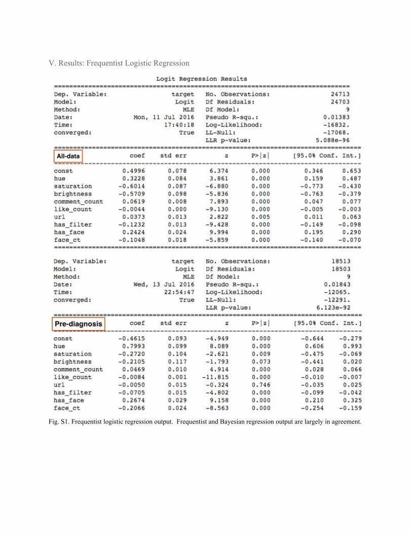
V. Results: Frequentist Logistic Regression

Fig. S1. Frequentist logistic regression output. Frequentist and Bayesian regression output are largely in agreement.

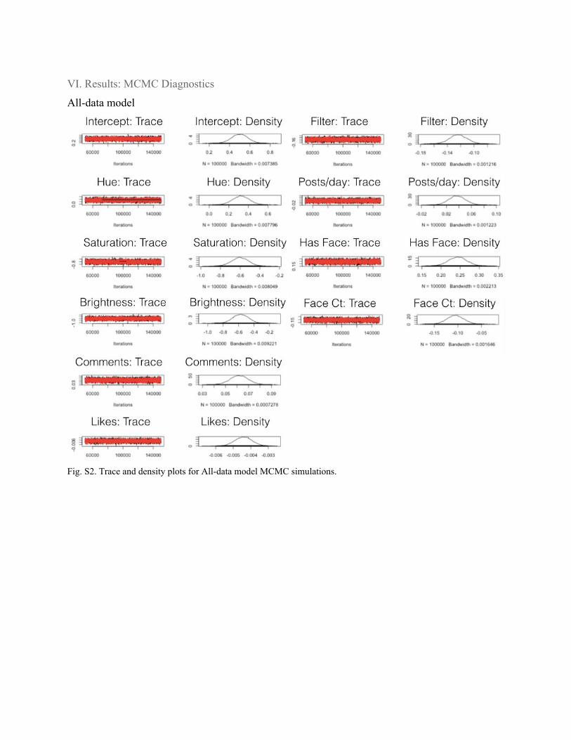
VI. Results: MCMC Diagnostics

All-data model

Fig. S2. Trace and density plots for All-data model MCMC simulations.

Fig. S3. Autocorrelation plot for All-data model MCMC simulations. First chain only is displayed for conciseness (second chain output is nearly identical). Pre-diagnosis model

Fig. S4. Trace and density plots for Pre-diagnosis model MCMC simulations.

Fig. S5. Autocorrelation plot for Pre-diagnosis model MCMC simulations. First chain only is displayed for conciseness (second chain output is nearly identical). Ratings model

Fig. S6. Trace and density plots for Ratings model MCMC simulations.

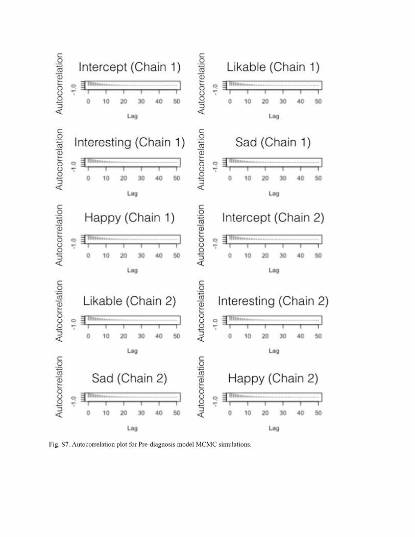
Fig. S7. Autocorrelation plot for Pre-diagnosis model MCMC simulations.

VII. Results: Bayesian regression

All-data model

Depressed μ (𝝈) Healthy μ (𝝈) Coef μ (𝝈) HPD Level HPD Interval

Intercept .500 (.080) 99% .298 .710

Hue .345 (.162) .338 (.157) .325 (.085) 99% .114 .547

Saturation .338 (.157) .347 (.155) -.602 (.087) 99% -.828 -.382

Brightness .535 (.138) .547 (.145) -.572 (.100) 99% -.835 -.321

Comments 1.077 (2.150) .992 (2.013) .062 (.008) 99% .042 .083

Likes 16.168 (34.874) 18.939 (34.214) -.004 (.005) 99% -.006 -.003

Posts/day 1.875 (1.961) 1.667 (1.775) .037 (.013) 99% .005 .072

Has filter .829 (1.108) .871 (1.524) -.124 (.013) 99% -.157 -.089

Has face .769 (1.137) .615 (.882) .243 (.024) 99% .181 .305

Face count .631 (.897) .623 (.984) -.105 (.018) 99% -.151 -.059

Table S2. Logistic regression output for All-data model1 (N=24,713). HPD Level = Highest Posterior Density Level, the probability that a regression coefficient falls within the given HPD Interval. HPD Levels listed are highest probabilities with which it can be claimed that a coefficient’s HPD Interval excludes zero.

Pre-diagnosis model

Depressed μ (𝝈) Healthy μ (𝝈) Coef μ (𝝈) HPD Level HPD Interval

Intercept .463 (.093) 99% -.695 -.211

Hue .360 (.166) .338 (.157) .802 (.099) 99% .545 1.054

Saturation .348 (.157) .347 (.155) -.271 (.104) 99% -.522 -.002

Brightness .534 (.136) .547 (.145) -.209 (.118) 90% -.410 -.026

Comments .912 (1.771) .992 (2.013) .047 (.010) 99% .023 .072

Likes 12.719 (28.912) 18.939 (34.214) -.008 (.001) 99% -.010 -.007

Posts/day 1.877 (1.931) 1.667 (1.775) -.004 (.015) 30% -.012 .000

Has filter .907 (1.191) .871 (1.524) -.071 (.015) 99% -.108 -.030

Has face .743 (1.030) .615 (.882) .267 (.029) 99% .189 .340

Face count .57 (.824) .623 (.984) -.207 (.024) 99% -.268 -.144

Table S3. Logistic regression output for Pre-diagnosis model ( N=18,513). HPD Level = Highest Posterior Density Level, the probability that a regression coefficient falls within the given HPD Interval. HPD Levels listed are highest probabilities with which it can be claimed that a coefficient’s HPD Interval excludes zero.

A posterior predictive check showed that All-data observations replicated from the joint posterior distribution consistently overestimated the proportion of depressed observations (replicated: 53.5% depressed; original: 30.9%), with a p-value of 1.0 . Pre-diagnosis observations sampled 1

from the joint posterior distribution slightly underestimated the proportion of depressed observations (replicated: 30.02% depressed; original: 37.97%), with a posterior predictive p-value of 0.039. Gelman et al. (48) suggested that a model with good replication accuracy should generate posterior predictive p-values within the range of 0.05-0.95. Note that an extreme posterior predictive p-value does not mean that a model is wrong, just that it fails to be “right enough” to render a reasonable replication of its input. All models nevertheless far outperformed a simple null model in the capacity to correctly predict class membership.

Depressed μ (𝝈) Healthy μ (𝝈) Coef μ (𝝈) HPD Level HPD Interval

Intercept -2.374 (.175) 20% -.045 -.004

1 In the context of logistic regression, the posterior predictive p-value assesses the frequency with which samples drawn from the simulated posterior overpredicts reference class membership, compared to reference class prevalence in the original data.

Happy 2.300 (1.042) 2.511 (1.109) -.193 (.034) 99% -.279 -.105

Sad .840 (.598) .757 (.614) .100 (.039) 95% .024 .176

Likable 2.393 (.918) 2.514 (.952) .027 (.050) 35% .007 .052

Interesting 2.316 (.816) 2.367 (.859) .041 (.041) 65% .003 .080

Table S4. Logistic regression output for Ratings model (N=8,976). HPD Level = Highest Posterior Density Level, the probability that a regression coefficient falls within the given HPD Interval. HPD Levels listed are highest probabilities with which it can be claimed that a coefficient’s HPD Interval excludes zero.

A posterior predictive check of Ratings model showed that sample observations replicated from the joint posterior distribution accurately represented the true proportion of depressed observations (replicated: 44.2% depressed; original: 43.9%), with a posterior predictive p-value of 0.516.

VIII. Results: Instagram filter examples

Fig. S8. Examples of Inkwell and Valencia Instagram filters. Inkwell converts color photos to black-and-white, Valencia lightens tint. Depressed participants most favored Inkwell compared to healthy participants, Healthy participants most favored Valencia compared to depressed participants.

IX. Results: Correlation tables

All-data model

Hue Satur. Bright. Comm. Likes Posts Filter Face

Saturation .17

Brightness -.22 -.28

Comments -.07 -.05 .10

Likes -.09 -.10 .17 .55

Posts .05 .03 -.06 -.02 -.03

Has filter .12 .08 -.02 -.05 -.07 .56

Has face .03 .04 -.05 -.00 -.02 .69 .34

Face count .01 .04 -.03 .02 .00 -.02 -.01 .42

Table S5. Pearson’s product-moment correlation scores for All-data model features.

Pre-diagnosis model

Hue Satur. Bright. Comm. Likes Posts Filter Face

Saturation .16

Brightness -.22 -.27

Comments -.05 -.06 .14

Likes -.08 -.13 .23 .49

Posts .06 .03 -.06 -.04 -.06

Has filter .13 .09 -.03 -.04 -.08 .63

Has face .04 .05 -.05 -.01 -.05 .66 .39

Face count .01 .03 -.02 .03 -.01 -.02 -.02 .45

Table S6. Pearson’s product-moment correlation scores for Pre-diagnosis model features.

Ratings model

Happy Sad Likable Interest.

Sad -.41

Likable .79 -.29

Interesting .53 -.09 0.77

Hue .02 -.02 -.01 -.03

Saturation .02 -.07 -.02 -.04

Brightness .05 -.04 .04 .03

Posts -.02 .04 -.01 .02

Comments .00 .02 -.02 -.03

Likes .04 -.02 .05 .06

Has filter .03 .00 .02 .01

Has face .16 .05 .06 .00

Face count .25 -.10 .11 .02

Table S7. Pearson’s product-moment correlation scores for Ratings model features (columns) with ratings and computational features (rows).

X. Ratings inter-rater agreement

Rater agreement was measured by randomly selecting two raters from each photo, and computing Pearson’s product-moment correlation coefficient from the resulting vectors. To mitigate sampling bias, we ran a five-fold iteration of this process and averaged the resulting coefficients. Rater agreement showed positive correlations across all ratings categories ( for all values shown): , , , e 8p < 1 − 3 39rhappy = . 19rsad = . 17rinteresting = . 27rlikable = .