RIVER BANK EROSION PROCESSES ALONG THE LOWER

SHUSWAP RIVER

FINAL PROJECT REPORT Submitted to

Regional District of North Okanagan

October, 2014

Hilary Cameron and Bernard Bauer University of British Columbia Okanagan

ii

Executive Summary

The Lower Shuswap River is one of many rivers in the interior of British

Columbia experiencing chronic bank erosion, which leads to land loss, aquatic habitat

degradation, and water quality challenges. Local land owners believe that bank

erosion is due to the intense levels of recreational boating traffic during the summer,

which is an issue that has been identified as a serious management concern (Shuswap

River Watershed Sustainability Plan, 2014).

A field study conducted in 2013 (Laderoute and Bauer, 2013; Laderoute,

2014) quantified boat-related erosion along the Lower Shuswap River during the

primary boating period (July - August). The overriding objective of the current

research was to complement the earlier study by assessing the rate of bank erosion

during the spring freshet (May – July) and to assess the near-bank flow mechanisms

that may be responsible for erosion.

The primary hypothesis upon which this study hinges is that the period of

most substantial bank erosion during an annual cycle occurs during the spring freshet

rather than the summer boating period. Should the primary hypothesis prove

incorrect, then there would be greater reason to assert that boating traffic may be an

important cause of bank erosion along the Lower Shuswap River. Boating traffic was

monitored at upstream and downstream locations using remotely triggered cameras.

During the peak of the spring freshet, when shear stress values acting on the bank are

expected to be greatest, velocity profiles were measured and later used to solve for the

boundary shear stress acting on the bank. To track erosion rates, erosion pin and bank

profile measurements were continued from Laderoute and Bauer (2013).

This project report contains a comprehensive literature review (Chapter 2) that

describes natural processes associated with river meandering and bank erosion. The

remaining chapters describe the methods used (Chapter 3), the results including data

tables and figures (Chapter 4), and a brief discussion of the findings (Chapter 5). The

report should be ready in combination with the earlier work by Laderoute (2014),

which describes the mechanics of boat-wake-induced erosion in greater detail.

Overall, the data indicate the following:

iii

(1) the near-bank shear stresses during the spring freshet (high river stage) are too

small to initiate sediment motion by direct hydraulic action and therefore are not

sufficiently strong to cause erosion at the study site;

(2) the period between early to late July is associated with both rapid decrease in

discharge and rapid reduction in river stage as well as a significant increase in

boating traffic;

(3) during the July drawdown period, there appears to be a discernible tendency for

erosion of the upper bank regions and sediment deposition on the lower bank

'aprons' or 'terraces';

(4) during August, the lower bank 'aprons' are scoured free of sediment deposits by

repetitive boat-wake waves whereas the upper bank regions are not affected by

wave action because the water levels are too low;

(5) the influence of boats in late August and early September declines markedly

because shallow water precludes the use of the lower reaches of the river for

recreational purposes other than kayaking and canoeing, and

(6) for the majority of the year (September – May) the river banks are not affected by

river flows or boat wakes because the water levels are too low to produce

significant stresses on the bank materials, although subaerial processes (e.g.,

freeze-thaw, runoff, vegetation growth, burrowing animals) may be active and

important.

iv

Acknowledgements

The following landowners generously provided access to their properties:

Hermann and Louise Bruns (Wild Flight Farm)

Corinne De Ruiter (Springbend Farms)

John and Maryanne (The Old Mara Train Station B&B)

Lori and Leo Konge (Viking Farms)

Anna Page and Laura Frank (North Okanagan Regional District) have provided

generous time and encouragement for the project. They have played a key role in

ensuring that the project went forward.

Financial support for logistics and materials came from the Regional District of North

Okanagan. Ms. Cameron was supported by an Undergraduate Student Research

Award from the Natural Science and Engineering Research Council, Canada.

Additional financial support came from internal grants to Dr. Bauer from the

University of Brisith Columbia Okanagan.

Bob Harding (Fisheries and Oceans Canada) is thanked for providing the remote

cameras that allowed image capture of boat-wake traffic, and for general advice

regarding regional concerns.

v

Contents

Chapter 1 Introduction

Pages 1-2

Chapter 2 Literature Review

Pages 3-22

Chapter 3 Methods

Pages 23-40

Chapter 4 Results

Pages 41-72

Chapter 5 Discussion and Conclusions

Pages 74-81

Chapter 6 Bibliography Pages 82-86

1

1. Introduction The Shuswap River is the largest river that flows into Shuswap Lake, with a

drainage basin area of 1969 square kilometers and a total length of 195 km (Kramer,

2003). The Shuswap River is important ecologically, economically, and socially.

From the ecological standpoint, it hosts many fish species, is an important spawning

habitat for salmon and provides habitat to a number of threatened and endangered

species. Economically, the Shuswap River is used for hydroelectric power

generation, supports timber and agricultural resources and also brings tourists into the

region for recreational purposes, including boating, swimming, paddling and fishing.

Culturally and historically, the Shuswap River has been used by the Splatsin First

Nation peoples, who used the river as a transportation corridor as well as a source of

food (Shuswap Nation Tribal Council, 2014).

The Shuswap River is generally broken down into three sub-sections : the

Upper, Middle and Lower Shuswap River. The Lower Shuswap River is considered

to be the 75 km stretch of river that extends from Mabel Lake to Mara Lake. The

Lower Shuswap River floodplain largely consists of farmland, although it also hosts

the city of Enderby and other small urban areas such as Grindrod and Mara as well as

significant transportation infrastructure.

The Lower Shuswap River is representative of a number of rivers in the south-

central interior of BC that experience chronic bank erosion. Excessive erosion is

detrimental in so far as it can cause property damage, lead to water quality issues, and

undermine the integrity of aquatic and riparian ecosystems. Many believe that

recreational boating is increasing the natural erosion rate of the bank. However, it is

well known that rivers naturally sculpt and shape the landscape through which they

flow. Although human development is capable of progressively altering the dynamic

environment in which rivers perform work, it is important to determine if and how

river bank erosion has been altered by these activities.

During the summer of 2013, an intensive study was performed on a reach of

the Shuswap River near Mara, BC, by Laderoute and Bauer (2013). They assessed

the intensity of recreational boating activity and its impact on bank erosion by

monitoring boat traffic and tracking erosion rates at nine locations along the Lower

Shuswap River. Although their work showed a high volume of boat traffic and

2

consequent erosion during the summer season (July-September), the results regarding

the impact of boats relative to natural bank erosion are ambiguous because no

information was available on the erosive impact of the spring freshet (the annual high-

water period during snowmelt). The goal of the current study was to redress this

shortcoming by monitoring the near-bank flow conditions and resulting erosion from

late March through early September, which includes the spring freshet period, as well

as extending the bank erosion time series initiated last year.

The primary working hypothesis is that hydraulic action during the high flow

period causes substantial bank erosion that dominates the annual cycle of bank

change. If the field evidence indicates that erosion is negligible during the spring

freshet, then other mechanisms of bank erosion (e.g., boat wakes) must be implicated

as relatively more important. The results from this study will have important

ramifications for management strategies intended to minimize or mitigate the chronic

bank erosion challenge on the Lower Shuswap River.

3

2. Literature Review 1. Introduction

Riverbank erosion along the Lower Shuswap River is of concern for the local

community as it threatens to damage or degrade private property, public roads, fragile

ecosystems, and water quality. However, large and uncontrolled channel erosion

rates are not just a local problem. In fluvial systems, a very large portion of the

sediment in the water is supplied through erosion of the riverbanks (Gardiner, 1983).

In fact, as much as 85% of the sediment yield in a watershed can originate from

stream-bank erosion alone (Clark and Wynn, 2007). Every year in North America,

$16 billion is spent on water pollution damage caused by too much sediment in the

water, which ranks as the second biggest pollutant after bacteria (Clark and Wynn,

2007). Large sediment concentrations not only decrease water clarity in streams, but

can be damaging to aquatic ecosystems because it inhibits the ability of fish to find

food, reduce light availability for aquatic plants, decrease the amount of dissolved

oxygen in the water and change the water temperature (Laderoute and Bauer, 2013).

In British Columbia, there is large concern for increased sediment concentration in the

water because of its impact on salmon. Increased sediment loads of fine-grained

material reduce spawning potential and decrease the incubation habitat quality of

salmon (Nelitz et al., 2007). Salmon are very important economically, culturally and

ecologically to many regions in the Pacific Northwest. In order to improve water

quality management, it is necessary to improve channel erosion predictions, which

will make it possible to calculate the sediment load in the river (Clark and Wynn,

2007).

Bank erosion can also damage riparian habitat. The riparian zone is the

transitional zone between dry land and the water channel. The riparian zone is

important because it can enhance the water quality by trapping sediments and filtering

pollutants. It can also provide aquatic and terrestrial habitat, and produce shade,

which keeps water temperatures cool for fish. Damage to the riparian zone can create

a positive feedback loop by further increasing erosion rates because the roots of trees

and shrubs along the river bank provide internal bank strength (EPA, 2012).

Land loss due to bank erosion is of increasing concern for property owners.

For example, the Matanuska River in Alaska has eroded private properties over the

last few decades as well as a major regional highway and farmland (Curran and

4

McTeague, 2011). The financial burden falls on the local landowner whose physical

workload can increase by repairing their damaged property. The costs of preventing

erosion can also be substantial. The Alberta provincial government recently allocated

$116 million to flood erosion control to help repair the damage from the June 2013

floods and to prevent the impacts of future flood events (Water Canada, 2013). Due

to the expense involved with installing structures to decrease or reverse erosion

damage, perhaps the best strategy is to stop activities that are known to cause or

enhance erosion.

There are many factors that influence erosion rates but the most important

driving factor involves the fluid flow, including the magnitude, frequency and

variation in stream discharge. Fluid flow properties also include the shear stress

distribution that the flowing water exerts on the bank, the amount of turbulence in the

water and the presence of waves. Other factors that impact the degree of river bank

erosion is the bank material composition (the texture, sorting, stratification, chemistry

and cohesion of the soil), climate (rainfall patterns and freeze thaw cycles), biological

influences (root systems and animal activity such as burrowing), subsurface

hydrology (pore pressure, soil moisture), channel geometry (width, depth, slope, and

degree of bending of the channel) and human influences (urbanization, agriculture,

boating and bank protection structures) (Knighton, 1998). The majority of these

variables change over the longitudinal profile of the river or from season to season.

When and where the most intense erosion is likely to occur can be important for

setting up erosion prevention structures or giving warning to people for when it may

be dangerous to approach a river.

It is important to understand that rivers naturally change their form and

structure over time. Much effort has been put forth to derive relationships between

flow patterns, bank characteristics, and velocity profiles in order to roughly estimate

how river banks will erode. The remainder of this chapter will explain the natural

processes of meandering rivers and discuss modern research methods being used to

predict riverbank erosion.

2. River Dynamics and Bank Erosion

2.1 River Meandering

Rivers naturally erode their banks and change their morphology to reach

equilibrium with the ever-changing conditions imposed on the stream. In a rigid

5

channel, such as a bedrock channel, the variation in discharge has to be

accommodated within the physical dimensions of the fixed channel geometry,

typically by changes in the depth of flow or the speed at which water moves down the

channel. However, alluvial channels (i.e., those situated in floodplains with erodible

banks) can accommodate changes in the imposed discharge by eroding their banks or

the bed, and subsequently deposit the eroded materials in new locations. Meandering

rivers, such as the Shuswap River, are very common, typically along reaches where

there is a gentle slope and the bed and bank materials are erodible and cohesive.

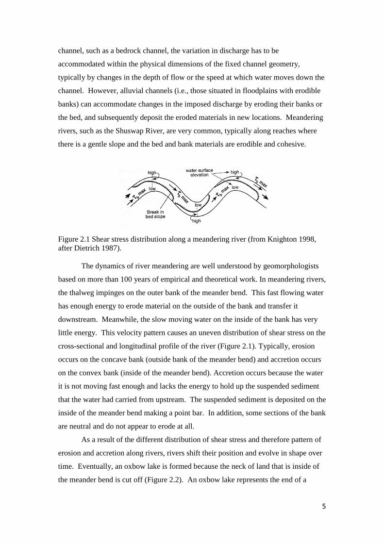
Figure 2.1 Shear stress distribution along a meandering river (from Knighton 1998, after Dietrich 1987).

The dynamics of river meandering are well understood by geomorphologists

based on more than 100 years of empirical and theoretical work. In meandering rivers,

the thalweg impinges on the outer bank of the meander bend. This fast flowing water

has enough energy to erode material on the outside of the bank and transfer it

downstream. Meanwhile, the slow moving water on the inside of the bank has very

little energy. This velocity pattern causes an uneven distribution of shear stress on the

cross-sectional and longitudinal profile of the river (Figure 2.1). Typically, erosion

occurs on the concave bank (outside bank of the meander bend) and accretion occurs

on the convex bank (inside of the meander bend). Accretion occurs because the water

it is not moving fast enough and lacks the energy to hold up the suspended sediment

that the water had carried from upstream. The suspended sediment is deposited on the

inside of the meander bend making a point bar. In addition, some sections of the bank

are neutral and do not appear to erode at all.

As a result of the different distribution of shear stress and therefore pattern of

erosion and accretion along rivers, rivers shift their position and evolve in shape over

time. Eventually, an oxbow lake is formed because the neck of land that is inside of

the meander bend is cut off (Figure 2.2). An oxbow lake represents the end of a

6

meandering cycle because after the neck is cut off, the river is straightened. In

straight channels, the thalweg still meanders back and forth, and eventually this leads

to a meandering path once again.

Figure 2.2 The formation of an Oxbow Lake from a meandering river (Gamesby, 2013).

2.2 Types of Bank Erosion

Bank erosion occurs through two dominant processes: hydraulic action and

mass failure (Posner and Duan, 2012). Hydraulic action entrains particles from the

bed and bank by the excess shear force exerted on the boundary by the flowing water.

The larger the water velocity, the greater the energy of the flow and the greater the

potential for hydraulic action to detach material from the bank. This material is

carried down the river until the water velocity slows down enough that it no longer

has the energy to suspend the particle.

Mass failure occurs when a large slab of material shears away from the bank

and slides or slumps to a lower position (Figure 2.3). This typically occurs when the

critical height and angle of the bank have been surpassed (Papanicolaou et al., 2007).

How prone a river bank is to mass failure depends on the geometry, structure and

material properties of the bank (Knighton, 1998). Slumping is a common form of

mass wasting in river banks that have cohesive material, which is the situation along

the Lower Shuswap River. Slumping usually occurs along concave upwards surfaces

when the bank materials are saturated or are experiencing rapid de-watering

(Trenhaile, 2010). If the base of the bank is undercut, the stabilizing forces of the

bank are decreased. Once the gravitational force becomes stronger than the forces

7

holding the bank together, a portion of the bank breaks off or begins to slip. A bank

is most susceptible to slumping when the water levels have declined but the bank is

still fully saturated (Trenhaile, 2010), as is the case after a storm event or soon after

the peak discharge of the spring freshet has passed (Figure 2.4).

Figure 2.3 Slumping caused by the undercutting of bank material on a river bank (Wikipedia: River bank failure, 2014, retrieved at: http://en.wikipedia.org/wiki/River_bank_failure).

Figure 2.4 Mass wasting event caused by a drop in river stage or a rise of the water table (Wikipedia: River bank failure, 2014, retrieved at: http://en.wikipedia.org/wiki/River_bank_failure).

Hydraulic action and mass failures are often interrelated. The hydraulic action

is associated with the shear stress exerted by the flow and is often concentrated at the

toe of the bank, resulting in undercutting of the bank. When the bank toe has been

8

eroded, and the bank height and angle are changed to the point where the gravitational

forces are larger than the forces holding the bank together, failure occurs (Simon et

al., 2009). This is depicted in Figure 2.5, where the bank toe is scoured out during

high water levels, which are often associated with increased shear stress. When water

levels drop, the overhanging material is now unstable due to the removed support.

Eventually, the overhanging material drops into the river and protects the lower bank

from further erosion until the hydraulic action removes this material once again

(Knighton, 1998). The strength of the hydraulic action may also be reduced after a

mass failure event because the newly fallen material may shift the flow away from the

bank (Kean and Smith, 2006a, 2006b). This can decrease the velocity gradient and

therefore reduce the shear stress. The bank retreat process is therefore a cyclical one

that alternates between an erosional stage dominated by hydraulic action followed by

geotechnical failures and slumping (Clark and Wynn, 2007).

Figure 2.5. Stream-bank retreat via mass failure and hydraulic action (TMDL, 2006).

2.3 Shear Stresses in a Water Channel

Erosion occurs when there is an imbalance of forces acting on a bed

comprised of erodible materials such as sand and silt. When the hydraulic forces

exceed the strength of the material on the bank, erosion takes place. The magnitude

and distribution of hydraulic shear stress on the bed of a natural channels has been

studied extensively over the years because the rate of bank erosion can be predicted

when the distribution of boundary shear stress is known (Kean et al., 2009).

The average shear stress on the bottom of an infinitely wide channel is given

by the tractive force equation:

τo = ɣRS (1)

9

Where τo is the mean boundary shear stress (given in N m-2), ɣ is the specific weight

of water (given in N m-3), R is the hydraulic radius of the stream (given in m) and S is

the slope of the stream (given in m m-1). However, when studying riverbank erosion,

the mean boundary shear stress value for the channel is often not suitable since the

distribution of shear stress is not equal along the cross section of the river. Therefore,

other methods that take the near bank flow processes into account are often more

appropriate.

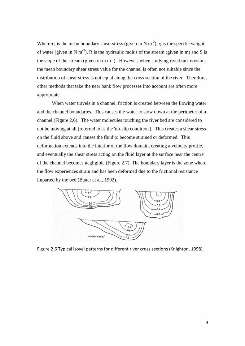
When water travels in a channel, friction is created between the flowing water

and the channel boundaries. This causes the water to slow down at the perimeter of a

channel (Figure 2.6). The water molecules touching the river bed are considered to

not be moving at all (referred to as the 'no-slip condition'). This creates a shear stress

on the fluid above and causes the fluid to become strained or deformed. This

deformation extends into the interior of the flow domain, creating a velocity profile,

and eventually the shear stress acting on the fluid layer at the surface near the centre

of the channel becomes negligible (Figure 2.7). The boundary layer is the zone where

the flow experiences strain and has been deformed due to the frictional resistance

imparted by the bed (Bauer et al., 1992).

Figure 2.6 Typical isovel patterns for different river cross sections (Knighton, 1998).

10

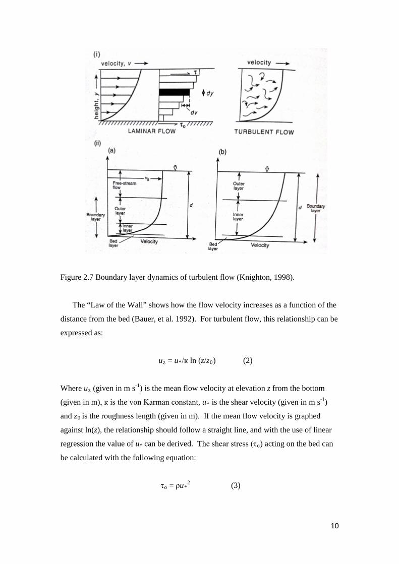
Figure 2.7 Boundary layer dynamics of turbulent flow (Knighton, 1998).

The “Law of the Wall” shows how the flow velocity increases as a function of the

distance from the bed (Bauer, et al. 1992). For turbulent flow, this relationship can be

expressed as:

uz = u*/к ln (z/z0) (2)

Where uz (given in m s-1) is the mean flow velocity at elevation z from the bottom

(given in m), к is the von Karman constant, u* is the shear velocity (given in m s-1)

and z0 is the roughness length (given in m). If the mean flow velocity is graphed

against ln(z), the relationship should follow a straight line, and with the use of linear

regression the value of u* can be derived. The shear stress (τo) acting on the bed can

be calculated with the following equation:

τo = ρu*2 (3)

11

where ρ is the density of water (given in kg m-3) and τo is the boundary shear stress

above the point where the velocity profile was measured (given in N m-2).

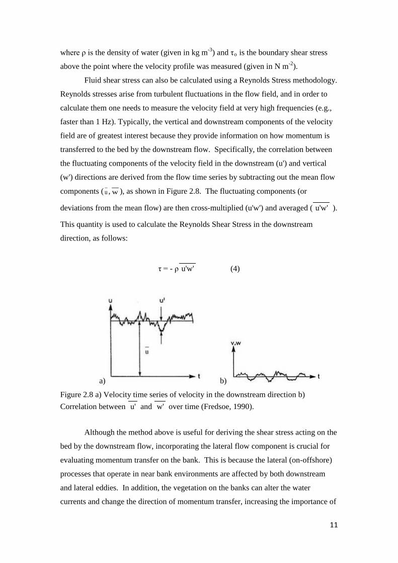
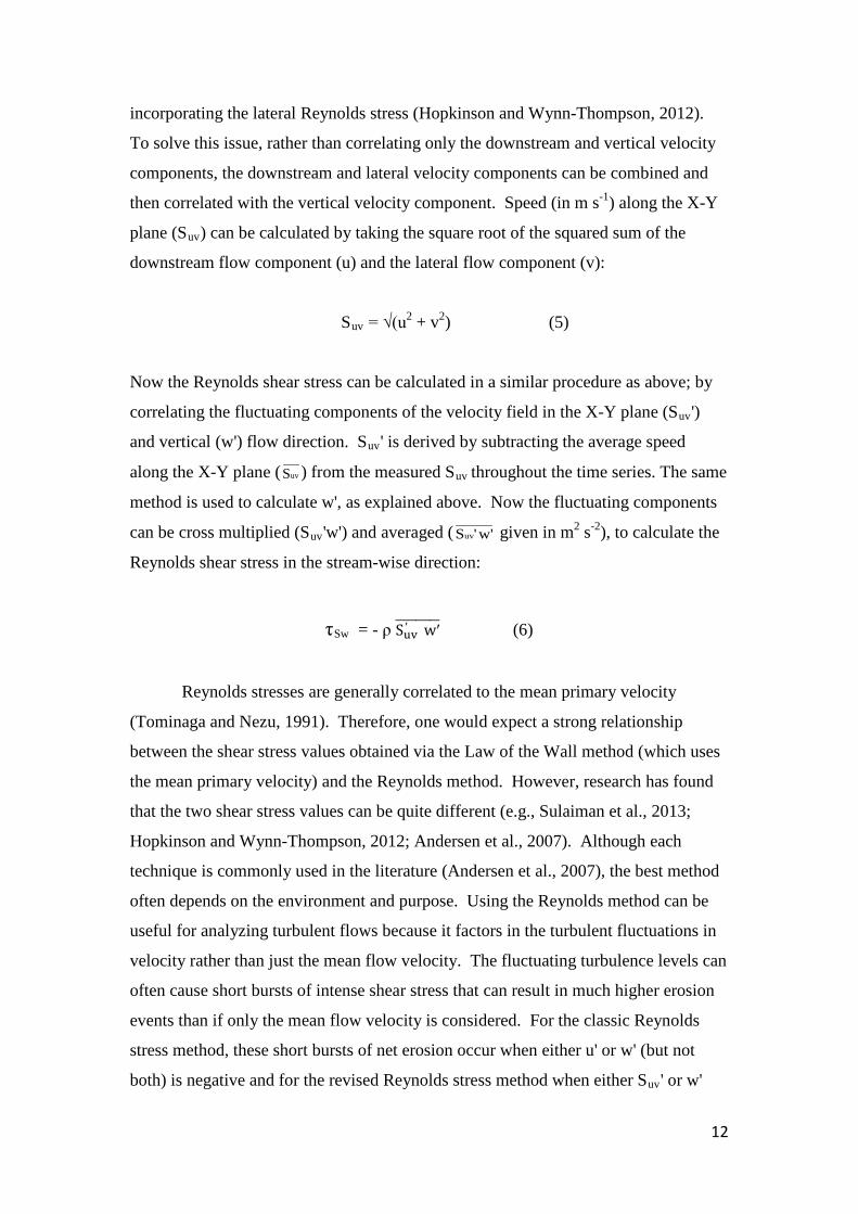
Fluid shear stress can also be calculated using a Reynolds Stress methodology.

Reynolds stresses arise from turbulent fluctuations in the flow field, and in order to

calculate them one needs to measure the velocity field at very high frequencies (e.g.,

faster than 1 Hz). Typically, the vertical and downstream components of the velocity

field are of greatest interest because they provide information on how momentum is

transferred to the bed by the downstream flow. Specifically, the correlation between

the fluctuating components of the velocity field in the downstream (u') and vertical

(w') directions are derived from the flow time series by subtracting out the mean flow

components ( u , w ), as shown in Figure 2.8. The fluctuating components (or

deviations from the mean flow) are then cross-multiplied (u'w') and averaged ( u'w' ).

This quantity is used to calculate the Reynolds Shear Stress in the downstream

direction, as follows:

τ = - ρ u'w' (4)

a) b)

Figure 2.8 a) Velocity time series of velocity in the downstream direction b) Correlation between u' and w' over time (Fredsoe, 1990).

Although the method above is useful for deriving the shear stress acting on the

bed by the downstream flow, incorporating the lateral flow component is crucial for

evaluating momentum transfer on the bank. This is because the lateral (on-offshore)

processes that operate in near bank environments are affected by both downstream

and lateral eddies. In addition, the vegetation on the banks can alter the water

currents and change the direction of momentum transfer, increasing the importance of

12

incorporating the lateral Reynolds stress (Hopkinson and Wynn-Thompson, 2012).

To solve this issue, rather than correlating only the downstream and vertical velocity

components, the downstream and lateral velocity components can be combined and

then correlated with the vertical velocity component. Speed (in m s-1) along the X-Y

plane (Suv) can be calculated by taking the square root of the squared sum of the

downstream flow component (u) and the lateral flow component (v):

Suv = √(u2 + v2) (5)

Now the Reynolds shear stress can be calculated in a similar procedure as above; by

correlating the fluctuating components of the velocity field in the X-Y plane (Suv')

and vertical (w') flow direction. Suv' is derived by subtracting the average speed

along the X-Y plane ( uvS ) from the measured Suv throughout the time series. The same

method is used to calculate w', as explained above. Now the fluctuating components

can be cross multiplied (Suv'w') and averaged ( w''Suv given in m2 s-2), to calculate the

Reynolds shear stress in the stream-wise direction:

τSw = - ρ Suv ′ w′��������� (6)

Reynolds stresses are generally correlated to the mean primary velocity

(Tominaga and Nezu, 1991). Therefore, one would expect a strong relationship

between the shear stress values obtained via the Law of the Wall method (which uses

the mean primary velocity) and the Reynolds method. However, research has found

that the two shear stress values can be quite different (e.g., Sulaiman et al., 2013;

Hopkinson and Wynn-Thompson, 2012; Andersen et al., 2007). Although each

technique is commonly used in the literature (Andersen et al., 2007), the best method

often depends on the environment and purpose. Using the Reynolds method can be

useful for analyzing turbulent flows because it factors in the turbulent fluctuations in

velocity rather than just the mean flow velocity. The fluctuating turbulence levels can

often cause short bursts of intense shear stress that can result in much higher erosion

events than if only the mean flow velocity is considered. For the classic Reynolds

stress method, these short bursts of net erosion occur when either u' or w' (but not

both) is negative and for the revised Reynolds stress method when either Suv' or w'

13

(but not both) is large and negative. These erosive events are referred to as sweep and

ejection events. Ejection events tend to move sediment upwards into faster flows and

sweeping events move the flow and material downwards into slower moving flow

(Trenhaile, 2010). The magnitude and frequency of these sweep and ejection events

caused from turbulent flow also influences the amount of sediment entrainment that

occurs along a stream (Knighton, 1998). Factoring in turbulence can make a large

difference in certain environments because it can influence the amount of hydraulic

action and therefore the erosion rates (Knighton, 1998). Therefore, when studying

erosion rates and the rate of sediment transport, the spatial and temporal variations in

turbulent bursting events may be very important due to the high instantaneous shear

stresses involved (Trenhaile, 2010).

2.4 Primary and Secondary Circulation in Rivers

Although the flow in a channel is primarily in the downstream direction, there

can be vertical and horizontal components to the overall flow direction. These

variations from the main downstream direction are referred to as 'secondary' flows or

'secondary' circulation patterns. Meandering reaches of rivers, for example, usually

have a helicoidal flow pattern which resembles a spiral. Figure 2.9 shows the

secondary current pattern formed at the cross section of a river with helicoidal flow.

The secondary current is produced by the curvature of the channel and from the

vertical velocity gradient of the primary flow (Kitanidis and Kennedy, 1984). When

the flow reaches a meander bend in a channel, the water is pushed to the outside bank

due to the centrifugal force. This creates a pressure gradient between the concave

(outside) and convex (inside) banks. However, due to the friction acting on the water

by the river bank, this centrifugal force is smaller near the bottom of the bank than at

the top of the bank (Einstein, 1926). In the boundary layer, the pressure gradient is

stronger than the centrifugal force. This balance of forces results in the circular flow

pattern that becomes superimposed on the primary flow, generating the helicoidal

flow and migrating thalweg that is seen in rivers.

14

Figure 2.9 Helicoidal flow present in a river bend (Knighton, 1998 after Markham and Thorne, 1992). The tilt of the water surface is grossly exaggerated in this diagram.

Secondary currents influence the formation of meandering rivers because they

shift the distribution of shear stresses along the river channel. As discussed earlier,

the amount of erosion that takes place depends on the strength of hydraulic shear

stress. When the stronger, faster primary flow is pushed to the concave banks of a

channel bend, more erosion takes place compared to the inside banks because the

velocity gradient is larger (Kitanidis and Kennedy, 1984; Einstein, 1926).

Furthermore, the erosion is strongest on the bottom section of the concave bank,

which results in an asymmetric cross section (Einstein, 1926). This undercutting of

the bank also promotes mass wasting events. As the faster thalweg impinges on the

outer banks, the slower and less powerful flow sticks to the inside of the bank and

often deposits material, creating a point bar. These forces result in the formation of

meandering rivers and eventually oxbow lakes.

In order to predict erosion rates, secondary currents need to be accounted for,

as it alters the distribution of shear stress along natural channels. Secondary currents

are often developed in the junction region between the floodplain and the main

channel (Tominaga and Nezu, 1991). However, for simplicity sake, the impacts of

secondary currents on shear stress are often not included in scientific studies. Results

from the Kean et al. (2009) model, which under-predicted the shear stress distribution

by about twenty percent, demonstrate the importance of applying the secondary

circulation effects in near bank shear stress analyses. In addition, Papanicolaou et al.

(2007) found that the sidewall shear stress value increased by a factor of two to five

when secondary currents were accounted for, compared to the classic Reynolds

method (equation 4). The influence of lateral flow can be incorporated into the

Reynolds method by combining the downstream and lateral flow variations into one

vector (via equation 5).

15

2.5 Initiation of Particle Motion

In locations along the river where the shear stress due to the flowing water

becomes strong enough to exceed the tendency for bed particles to sit on the bottom,

the initiation of particle motion (or sediment transport) begins (McCuen, 2004). The

critical condition occurs when the stabilizing forces (gravity and packing of the

material) equal the mobilizing forces (the fluid drag, fluid lift and particle impacts).

Theoretically, the critical shear stress can be found using the Shields diagram (Figure

2.10), which relates the dimensionless critical shear stress (θ) to the boundary

Reynolds number (Re*). The dimensionless critical shear stress is defined as:

θ = τcr/g(ρs-ρ)D (7)

where g is the gravity constant (equal to 9.81 m s-1), ρs is the density of the sediment

(given in kg m-3), ρ is the density of the fluid (given in kg m-3), D is the diameter of

the particle (given in m), and τcr is the actual critical shear stress. The boundary

Reynolds number (Re*) depends on the diameter of the particle (D), the shear velocity

(u*) and the kinematic viscosity (v in m2 s-1):

Re* = u*D/v (8)

Figure 2.10 The Shields Diagram (after Shields, 1936).

16

Given the values for a range of system parameters such as grain size, flow

velocity, and fluid properties, it will be possible to predict the value of the critical

shear stress using the Shields diagram. The critical value can then be compared to the

calculated shear stress from Equations 1, 3 or 4 to determine whether sediment

entrainment is likely and therefore if erosion is likely to occur.

Although the Shields curve appears as a single line, it should be interpreted as

a region or zone for which sediment entrainment may happen. This is due to a number

of reasons. For one, the derivation of the curve assumes that all the particles are the

same size (Knighton, 1998). This is certainly not the case in most riverbanks as there

is usually a variety of shapes and sizes for the bank material. Typically, the mean

grain size is used and it is assumed that the system behaves as if it were comprised of

a uniform size of equivalent diameter. Also, there are varying definitions of when a

particle begins to move, making the precise moment of particle movement somewhat

subjective (Clark and Wynn, 2007). Many researchers have classified the point of

failure based on different observed characteristics such as the cloudiness of the water

or when the soil of the surface becomes pitted (Clark and Wynn, 2007). Furthermore,

the theory assumes steady flows, which is not the case in the majority of natural

rivers. And finally, the turbulence in the water can result in instantaneous stresses

that are much greater than the average, resulting in erosion at lower-than-predicted

mean shear stress values (Knighton, 1998). Because of this, the fine scales of

turbulent forces must be evaluated in order to gain a greater understanding of

sediment transport rates even if the threshold limit is not reached (Sulaiman et al.,

2013).

Finally, it needs to be appreciated that the Shields diagram does not strictly

apply to cohesive sediment such as those found in river banks along meandering

reaches (Debnath et al., 2007). Even though the boundary shear stress can be

quantified for very fine grained materials such as silts and clays, these values may not

apply. Therefore it will be difficult to calculate erosion rates due to a lack of

understanding of the actual shear strength of the bank material when particle cohesion

is at play. There are several models that can be used to estimate the critical shear

strength of cohesive materials based on such parameters as the percent clay of the

soil, the plasticity index and the average particle size of the material. However, these

different methods often yield very different values for critical shear stress (Clark and

Wynn, 2007).

17

2.6 Bank Erodibility

Stream bank erosion depends on the balance between the erodibility of the

material and the hydraulic/geotechnical forces applied to the bank (EPA, 2012). As

mentioned above, predicting the rate of erosion becomes very difficult in

circumstances where cohesive bank materials are involved because it is challenging to

estimate the strength of cohesive sediments. Electrochemical bonds between the clay

particles make them more resistant to erosion in comparison to non-cohesive sand

sized particles. Therefore, the Shields diagram tends to underestimate the critical

shear stress value for cohesive material (Clark and Wynn, 2007). The consequence of

this is that the Shields diagram offers only a crude means by which to estimate the

critical shear stress for cohesive material.

Another confounding factor is due to the varying properties of the bank

materials, including the moisture content, mineralogy, packing, porosity,

stratification, and bank geometry (Knighton, 1998). Thus, the resistance of cohesive

material to shear stress is often site dependent and very localized. It can also change

throughout the year based on flooding and storm events interspersed with dry periods

or periods of freezing temperatures. Many researchers overcome the challenge by

taking large samples of the bank and placing them in flumes to measure the critical

shear stress of their studied bank material directly.

The presence of roughness elements on the bed (e.g., ripples and dunes) and

bank (e.g., slump blocks) can also affect the shear stress distribution and therefore the

dislodgement of particles. The total bottom stress partially acts on the particles as

skin friction and on the roughness elements (such as vegetation and bed forms) as

form drag. Only the skin friction component of the total bottom stress acts on the

particles and causes erosion and sediment transport. Therefore, the more shear stress

acting on the roughness elements the less shear stress is acting on the soil particles

and the less energy is available for erosion. Small topographic changes in the bank,

often due to slumping events, can also cause form drag which can significantly alter

the flow in the river channel (Kean and Smith, 2006a). This means that large mass

wasting events can result in a negative feedback loop through which the overall

stability of the bank is increased because the slump blocks form elements that absorb

the majority of the shear stress in the flow.

The amount and density of vegetation in the flow greatly influences the degree

of form drag along the bank and therefore reduces the amount of total bottom shear

18

stress available to erode the soil. Significant reduction in particle shear stress can be

seen in surfaces only partially covered in vegetation (Thompson et al., 2004). When

studying bank erosion rates in natural channels, factoring in riparian and aquatic

vegetation may be necessary because the amount of shear stress partitioning can

significantly change stream bank erosion rates (Clark and Wynn, 2007). Furthermore,

a biofilm layer covering the perimeter of the channel or sections of the channel can

have a pronounced impact on the resistance to erosion (Andersen et al., 2007). A

biofilm layer is simply a layer of microorganisms that cover a surface which may act

as a sort of armor that can withstand strong shear stresses before being eroded to

reveal the soil underneath (Andersen et al., 2007).

Another factor affecting erosion rates in meandering channels is the layering

of bank material or the stratigraphy. The vertical changes in the physical properties

throughout the bank may make certain sections more subject to erosion. Wojda

(2008) found that bank material analyzed in a laboratory flume would erode in

distinct layers based on the erodibility of each layer. If the underlying layers are more

easily eroded, it can promote mass wasting due to the undercutting of the bank.

Streambeds may also be more resistant to erosion than stream banks because they are

not exposed to sub aerial processes and are always submerged underwater (Clark and

Wynn, 2007). This causes rivers to migrate laterally faster than vertically.

Due to all the variables that influence bank resistance to erosion, it is often

difficult to determine the critical value of shear stress needed to yield bank erosion,

especially for cohesive materials. Therefore, when studying natural channels, in situ

measurements of critical shear stress are often preferable because it is difficult to

transfer the bed or bank material to the flume without disturbing some of the many

factors that affect erosion resistance (Clark and Wynn, 2007).

2.7 Spatial and Temporal Aspects of River Erosion

The general shape of the channel and depth of water will affect how a stream

will erode. In meandering rivers, the outer bank of a meander bend has a steep

velocity gradient and therefore high shear stress. As a consequence, the outside bank

should experience greater erosion rates in comparison to the inside bank (Knighton,

1998). Bank angle and curvature also affect how stable the bank is and therefore how

fast it will retreat. Curran and McTeague (2011) found that aggressive bank erosion

along the Matanuska River in South-central Alaska was correlated more to bank

19

height and composition than the flow characteristics. Also, the height of the

floodplain relative to the water level can affect the rate of erosion. Tominagan and

Nezu (1991) performed a flume experiment and discovered that as the height of the

floodplain increases relative to the water level, the bed shear stresses decrease. The

height of the floodplain can also alter the structure of the secondary currents, which

can further impact the rate of erosion (Tominagan and Nezu, 1991). Therefore, the

relative structure and location of the river on the longitudinal profile can impact the

erosion rates.

There are also a number of climate factors that can reduce the strength of the

bank material making it more vulnerable to bank erosion (Clark and Wynn, 2007). In

North America, where winters can be harsh and cold, a major factor that reduces the

soil strength is freeze-thaw action. This is where the water in the bank continuously

freezes and thaws during fluctuating temperatures. This can weaken the soil and

therefore decrease the critical shear stress value. When the spring melt-water enters

the fluvial system, it can easily erode the top layers of the bank because they have

been weakened over winter. Simon et al. (2009) found that the streams that bring

sediment to Lake Tahoe transfer the most material during the spring snowmelt period.

However, Gardiner (1983) who worked in Northern Ireland, also found strong

temporal variations in erosion rates but discovered the opposite phenomenon. He

found that it was during the summer period that the subaerial processes weakened the

soil and were thereby transferred away during the winter months. He also noticed that

especially on the upper portions of a riverbank, the formation of needle ice could be

the most prominent factor for determining erosion. These factors resulted in the

winter months having the greatest erosion rates throughout the year. The impacts of

seasonality can vary greatly.

Humans also impact bank erosion on a spatial and temporal scale.

Urbanization moves water after a storm faster into the fluvial system then would

naturally occur. This causes the discharge in the river to increase faster and stronger

than in an untouched environment. The strong shear stresses created from the

increased discharge can lead to increased bank erosion rates. The same issue occurs

with deforestation because more water is entering the fluvial system because it is not

being taken up or slowed down by the surrounding vegetation. In addition,

deforestation of the riparian zone can damage the stream bank stability.

20

Although there tends to be smaller erosion rates during low discharges, there

are so many variables that effect bank erosion rates that there is a rather weak

correlation between flow volume and amount the bank has retreated (Knighton,

1998). It is clear that there are many seasonal factors that affect bank erosion as well

as spatial. The general morphology of fluvial landforms changes in an attempt to

reach equilibrium with the surrounding conditions (Trenhaile, 2010). Thus,

depending on the climate, bank structure, vegetation, relief, frequency and magnitude

of flooding as well as the presence of boating, peak erosion rates may occur at

different times of the year and the geomorphology of rivers can be very diverse.

Therefore, erosion rates are often site-specific and year-long study periods or longer

may be necessary to capture the nature of bank erosion along a river reach.

3. Measuring and Modelling River Bank Erosion

Predicting the amount of erosion that will occur over time can be a

challenging undertaking. On a large scale, scientists commonly use aerial photographs

(e.g., Curran and McTeague, 2011; Constantine et al., 2009; Pizzuto and

Mackelnburg, 1989), which are acquired from platforms on planes or satellites. The

displacement of the meandering pattern can be tracked by referencing the changing

shape to fixed monuments or markers such as roads, railroad tracks, and fence lines.

Bank erosion rates can also be measured on smaller scales using simple

technologies such as erosion pins. Erosion pins consist of metal re-bar hammered

into the ground, which makes for a cheap, simple, accurate, and very portable

methodology. The amount of erosion (or accretion) can be monitored at regular

intervals (days to weeks) based on the length of rod that sticks out (or is buried) in the

bank. Topographic surveying is another common way to monitor small scale erosion.

In topographic surveying, the bank profile can be obtained by calculating the relative

elevation of the bank to a known elevation that will not change (referred to as a bench

mark). These surveys are accurate to about 0.02m and are useful because the bed

morphology of the entire channel can be monitored (Pizzuto and Meckelnburg, 1989).

Having reliable field data on bank erosion is essential in calibrating predictive

models of natural processes in rivers. Ikeda et al. (1981) showed theoretically that

river bank erosion can be linearly related to the excess near bank velocity. This is the

difference between the depth averaged velocity and the mean cross sectional velocity

of the channel. This simple model can predict river migration patterns reasonably

21

well, although there is often large error associated with model predictions (Posner and

Duan, 2012). Modern methods have built off and reformed the Ikeda et al. (1981)

model focusing more on the distribution of boundary shear stress along the channel

rather than just the variation in velocity. The boundary shear stress value can be used

to predict sediment transport and shoreline erosion in fluvial environments

(Hopkinson and Wynn-Thompson, 2012). One of the main mechanisms to predict the

erosion rate of fine grained material in a stream channel is by the excess shear stress

equation (Clark and Wynn, 2007):

ε = kd (τa − τc )a (9)

where ε is the erosion rate (given in m s-1), kd is the erodibility coefficient (given in

m3 N-1 s-1), a is an exponent (usually assumed to be 1), τa is the applied shear stress

(given in N m-2) and τc is the critical shear stress (given in N m-2). Current

measurement techniques limit τa to be estimated using velocity measurements and

then solving for shear stress by using methods such as the Law of the Wall or the

Reynolds method as discussed earlier. The most appropriate method depends on the

flow characteristics of the water.

Since the Ikeda et al. (1981) model was introduced, numerous bank erosion

models have been developed in an attempt to predict erosion rates based on bank and

flow characteristics. Today, analyses of bank erosion are often performed in

laboratory flumes, which are man-made channels intended to represent natural rivers

(e.g., Hopkinson and Wynn-Thompson, 2012; Kean et al., 2009; Clark and Wynn,

2007; Czernuszenko and Holley, 2007; Debnath et al, 2007; Papanicolaou et al.,

2007; Thompson et al., 2004; Song and Chiew, 2001; Tominaga and Nezu, 1991).

Flumes are useful because a number of variables (such as bank material and structure,

flow characteristics, and channel geometries) can be controlled. However, diligence

must be maintained when applying results from these experiments to natural channels.

This is because natural channels do not have the simple, smooth, channel geometries

that flumes have and rarely have uniform flow, which is used in laboratory

experiments (Papanicolaou et al. 2007). Also, when bank materials are tested in the

lab, the properties of the cohesive materials can significantly change when they are

transported from the field to the laboratory (Debnath et al, 2007).

22

Despite the difficulty in understanding channel migration, there is a growing

interest for investors, property owners, and municipal and provincial governments to

understand the physical flow properties of water. Modern models try to incorporate

many variables, such as bank composition, bank height and flow characteristics to

estimate the boundary shear stress that is exerted on the bank by flow. However, little

work has been done to test these models in the natural environment. Therefore, there

is a need for scientific testing to analyze the accuracy of these predictive models and

to gain a greater knowledge on how fluid flow properties change the landscape.

23

3. Methods 3.1 Overview

Multiple methods were used to investigate erosion processes along the banks

of the Lower Shuswap River. Long-term bank erosion was monitored from the spring

to the fall with the use of erosion pins and standard surveying methods. Changes in

the bank profiles were evaluated in light of boating traffic patterns and shear stress

intensity measurements during the spring freshet and subsequent summer season. A

detailed topographic analysis was conducted on a portion of the bank to capture

characteristic features of the banks along the Lower Shuswap River.

3.2 Long-Term Bank Erosion Monitoring

Laderoute and Bauer (2013) installed a network of erosion pins at several sites

along the Lower Shuswap River in May 2013, which were reoccupied and continually

monitored during 2014. Erosion pins are long pieces of re-bar that are installed either

vertically (V) or horizontally (H) along the bank. They are hammered into the bank

so that the tip of the re-bar is flush with the ground surface. The progressive exposure

or burial of the re-bar during a given time increment correlates to the rate of erosion

or accretion, respectively. Typically, horizontal pins show progressive erosion only

unless a major bank slumping event occurs that buries the pin. In contrast, vertical

pins show erosion during periods of bank scour, but also sediment accumulation on

top of the pin when eroded material from higher on the bank settles on the lower bank

apron. A detailed explanation of the erosion-pin installation procedure can be found

in Chapter 3 of Laderoute (2014).

Five sites were selected to conduct the erosion pin experiments between

Enderby and Mara, British Columbia. These five sites were located on the Cox, De

Ruiter, Stewart, Konge and Bruns properties. The location of these sites along the

Lower Shuswap River is shown in Figure 3.1.

24

Figure 3.1 The five erosion pin sites containing nine erosion pin profile lines along the Lower Shuswap River as it flows into Mara Lake (from Laderoute, 2014).

The Cox Site was used as the control site because it is protected from boat

wakes by a long mid-channel island. The bank is further protected by thick vegetation

on the bank and is composed of mud and silt deposits. These features reflect the main

characteristics of banks along the Lower Shuswap River. Because the site is not

strongly influenced by boats, it should represent accurately the seasonal bank changes

that take place due to natural processes, including the spring freshet. The site is

located immediately downstream of the Mara Bridge on river left.

The De Ruiter Site is the most upstream site, located on the entrance to a large

meander bend on river left. The banks are steep and there is abundant vegetation,

including a number of large cottonwood trees. Compared to the rest of the sites, it

experiences the least boating traffic due to its distance from Mara Lake.

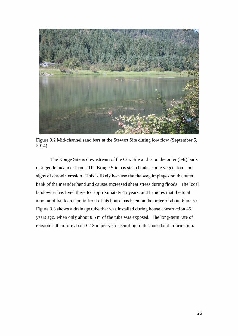
The Stewart property is located upstream of the Mara Bridge and next to River

Side Road, on river right of a straight reach. It has gently sloping banks and

vegetation. There are many shallow sand bars adjacent to the Stewart Site that pose a

hazard to boaters during low flows. These can be seen in Figure 3.2 in the middle of

the channel at low flow when the tops of the bars are exposed.

25

Figure 3.2 Mid-channel sand bars at the Stewart Site during low flow (September 5, 2014).

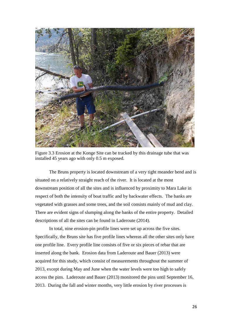
The Konge Site is downstream of the Cox Site and is on the outer (left) bank

of a gentle meander bend. The Konge Site has steep banks, some vegetation, and

signs of chronic erosion. This is likely because the thalweg impinges on the outer

bank of the meander bend and causes increased shear stress during floods. The local

landowner has lived there for approximately 45 years, and he notes that the total

amount of bank erosion in front of his house has been on the order of about 6 metres.

Figure 3.3 shows a drainage tube that was installed during house construction 45

years ago, when only about 0.5 m of the tube was exposed. The long-term rate of

erosion is therefore about 0.13 m per year according to this anecdotal information.

26

Figure 3.3 Erosion at the Konge Site can be tracked by this drainage tube that was installed 45 years ago with only 0.5 m exposed.

The Bruns property is located downstream of a very tight meander bend and is

situated on a relatively straight reach of the river. It is located at the most

downstream position of all the sites and is influenced by proximity to Mara Lake in

respect of both the intensity of boat traffic and by backwater effects. The banks are

vegetated with grasses and some trees, and the soil consists mainly of mud and clay.

There are evident signs of slumping along the banks of the entire property. Detailed

descriptions of all the sites can be found in Laderoute (2014).

In total, nine erosion-pin profile lines were set up across the five sites.

Specifically, the Bruns site has five profile lines whereas all the other sites only have

one profile line. Every profile line consists of five or six pieces of rebar that are

inserted along the bank. Erosion data from Laderoute and Bauer (2013) were

acquired for this study, which consist of measurements throughout the summer of

2013, except during May and June when the water levels were too high to safely

access the pins. Laderoute and Bauer (2013) monitored the pins until September 16,

2013. During the fall and winter months, very little erosion by river processes is

27

expected because of the low water levels. In addition, there was substantial snow and

ice cover, and therefore erosion rates could not be monitored.

The erosion pins were measured again on March 21, 2014 to assess the degree

of erosion that took place over the winter months, if at all. These data prior to the

spring freshet provide a baseline against which to assess the amount of erosion during

the subsequent flooding season. Because of high water levels during April, May, and

June, further access to the pins was not possible until July 25, 2014, when only the

upper erosion pins could be accessed safely. The erosion pins were then monitored

on a regular basis to check for changes in bank elevation during the remainder of the

summer.

3.3 Long-Term Boat Traffic Monitoring

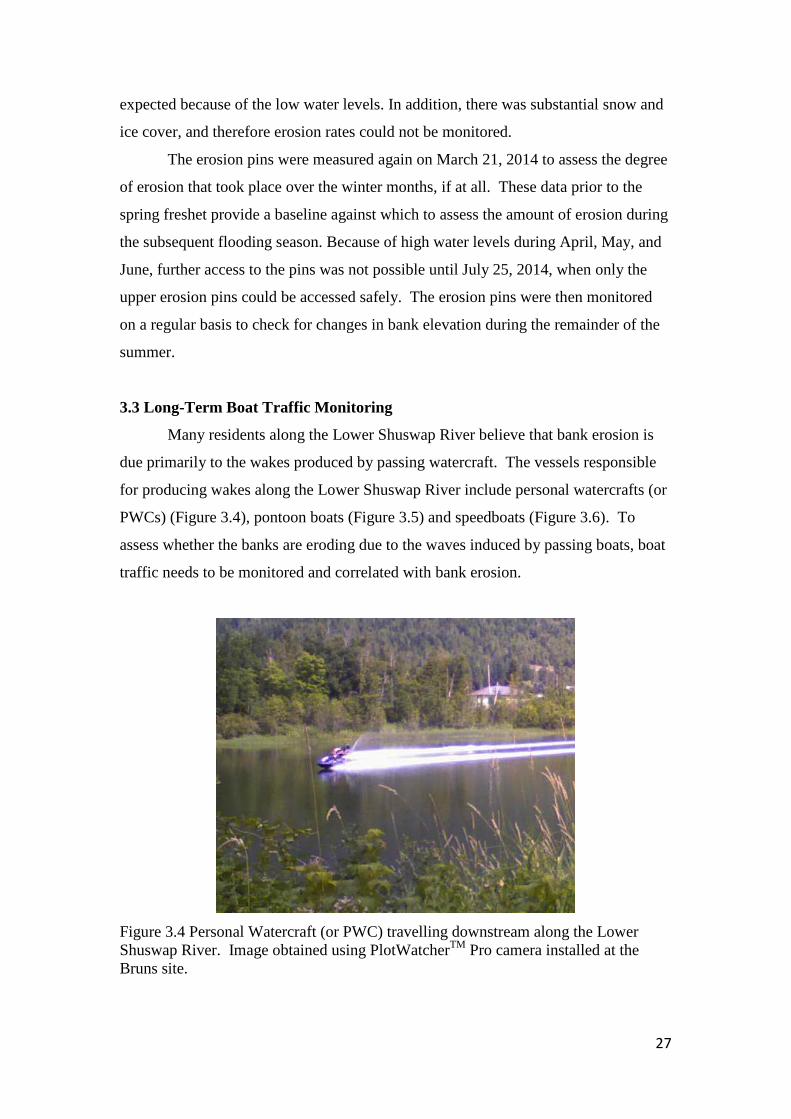
Many residents along the Lower Shuswap River believe that bank erosion is

due primarily to the wakes produced by passing watercraft. The vessels responsible

for producing wakes along the Lower Shuswap River include personal watercrafts (or

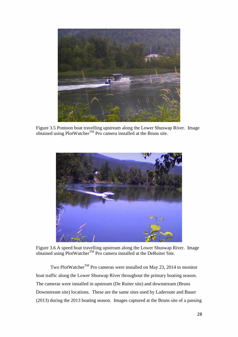
PWCs) (Figure 3.4), pontoon boats (Figure 3.5) and speedboats (Figure 3.6). To

assess whether the banks are eroding due to the waves induced by passing boats, boat

traffic needs to be monitored and correlated with bank erosion.

Figure 3.4 Personal Watercraft (or PWC) travelling downstream along the Lower Shuswap River. Image obtained using PlotWatcherTM Pro camera installed at the Bruns site.

28

Figure 3.5 Pontoon boat travelling upstream along the Lower Shuswap River. Image obtained using PlotWatcherTM Pro camera installed at the Bruns site.

Figure 3.6 A speed boat travelling upstream along the Lower Shuswap River. Image obtained using PlotWatcherTM Pro camera installed at the DeRuiter Site.

Two PlotWatcherTM Pro cameras were installed on May 23, 2014 to monitor

boat traffic along the Lower Shuswap River throughout the primary boating season.

The cameras were installed in upstream (De Ruiter site) and downstream (Bruns

Downstream site) locations. These are the same sites used by Laderoute and Bauer

(2013) during the 2013 boating season. Images captured at the Bruns site of a passing

29

PWC and pontoon boat can be seen in Figure 3.4 and Figure 3.5 respectively and an

image of a speedboat passing at the DeRuiter site can be seen in Figure 3.6.

Laderoute and Bauer (2013) observed many more boats at the Bruns site than the

DeRuiter site, and they suggested that tourists and lake residents often travel up the

Shuswap River to explore or to use the calmer waters that are ideal for water skiing

and other recreational water sports. The DeRuiter property is much farther upstream

and likely does not receive as much traffic originating from Mara Lake, although the

boat launch located in Enderby provides an additional source of boats.

The cameras ran from 5:00 to 22:00 every day and took a still picture every 3

seconds. At this capture rate, a 32 GB memory card filled in about 10 days. Initially,

the memory cards were switched every one and a half weeks. However, during mid-

June we were unable to service the cameras in time, and some of the images from

June 18-21 were over-written. In September, the camera at the Bruns site failed to

trigger, so there is another brief period for which boat images are not available.

Fortunately, the boating intensity was minimal during these periods; in June because

the freshet was at its peak and the boating season had not really begun yet, whereas in

September because the water was too shallow for safe boating to take place in the

river. The lack of data for these days will not have a significant impact on the total

traffic intensity estimates.

The photos captured with the PlotWatcherTM Pro cameras were viewed in fast

succession on a program called GameFinderTM. An image was saved for every

passing boat. In addition, the time the boat passed the camera location, direction the

vessel was travelling and type of watercraft were recorded in a spreadsheet. This

allows the intensity of boat traffic to be related to erosion rates as well as to assess

where the boats originate from (presuming round trips).

3.4 Short-Term Water Velocity and Turbulence Monitoring

Natural rivers are often dominated by turbulent and fluctuating flow. The

degree of turbulence can impact the rate of bank erosion because it can increase the

amount of shear stress. The amount of shear stress acting on the bed or bank can be

calculated using the Law of the Wall method (Equations 2 and 3) or using the

Reynolds Stress method (Equation 4 and 6). Both of these methods require velocity

measurements. The Bruns property was chosen to monitor the flow velocity of the

Lower Shuswap River during the spring freshet to correlate the calculated shear stress

30

values with erosion rates. The Bruns site was easy to access by road and the property

owners were willing to accommodate us during the experiments. The site also has

characteristic bank features for the lower reaches of the river as it shows significant

signs of bank slumping and the property consists of sparsely spaced trees with thick

grass vegetation. Figure 3.7 shows a picture of the Bruns Middle Site with the two

middle erosion pin profiles during installation (May 2, 2013).

Figure 3.7 Bruns Middle Site. Note substantial slumping features on the bank.

In March 2014, a measurement station was set up near the Bruns Middle Site

to record velocity profiles along the bank in order to derive values for shear stress.

The measuring station was composed of two sets of scaffolding stacked on each other.

Sets of concrete bricks were emplaced into the bank where the corners of the

scaffolding were to be located. Velocity profiles were measured using a Velocimeter

at locations between the left and right sets of bricks seen in Figure 3.8. Figure 3.9

shows the measurement station sitting on top of the bricks during higher water flow.

The purpose of using the concrete bricks was to prevent the scaffolding from sinking

into the bank over time and to keep the structure relatively level. Plywood was laid

down and tied to the scaffolding to act as a platform.

31

Figure 3.8 Velocity profile measurements were taken between the left and right cement blocks to monitor shear stress acting on the river bank along the Bruns Property. The photo shows the upstream direction and the two upstream brick pairs.

Figure 3.9 Scaffolding platform used to support the instruments during collection of velocity data on May 22nd, 2014. View is in the downstream direction.

32

A SonTek Field Acoustic Doppler Velocimeter (ADV) was installed on a rack

that was attached to the scaffolding. The rack had several sliding components that

enabled accurate positioning of the ADV, and these sliding components were

accurately levelled during the installation process. The ADV probe has a transmitter

and three receivers. The transmitter sends out an acoustic signal and the velocity is

measured based on the Doppler effect. Because turbulent flow is so complicated,

very precise and accurate instruments are needed to analyse the water flow. An ADV

is an ideal instrument to use to analyse flow characteristics because it can collect data

at very high frequencies (25 Hz) and uses a small sample volume. This is useful

because it allows turbulent eddies in the water to be analysed at high resolution

(Voulgaris and Trowbridge, 1997). The ADV is capable of collecting the velocity

data of a turbulent flow along the three Cartesian coordinates (X, Y, Z) as well as

calculating the distance from the sample to the boundary surface. This is useful for

establishing the velocity profile.

The rack attached to the scaffolding allowed the ADV to be moved left, right,

up and down on level angle iron. A picture of the set up can be seen in Figure 3.9.

Extra care had to be taken in mounting the instrument because if it is not aligned

properly, it can impact the calculated shear stress results (Andersen et al., 2007). The

ADV was oriented so that the positive x-axis aligned with the downstream direction,

the positive y-axis was in the transverse direction pointing towards the bank and the

z-axis was in the vertical direction with the positive axis pointed upwards.

The Bruns Middle Site offers the characteristic bank features displayed

throughout the Lower Shuswap River. Bank slumping is very prominent at the Bruns

property and although the section of the bank used to set up the measuring station had

few distinctive characteristics relative to the rest of the property, the chosen location

resembled the remnants of slumping events. As seen in Figure 3.8, a large portion of

the bank was missing and has been eroded away over time, resulting in a section with

fairly flat topography. This location was chosen because the scaffolding could be

easily installed relative to other sections of the bank. However, it was also at a

slightly lower elevation compared to just upstream of the scaffolding. There is about

a 0.3 m step in bed elevation between where the measurements took place and about

0.5 m upstream.

33

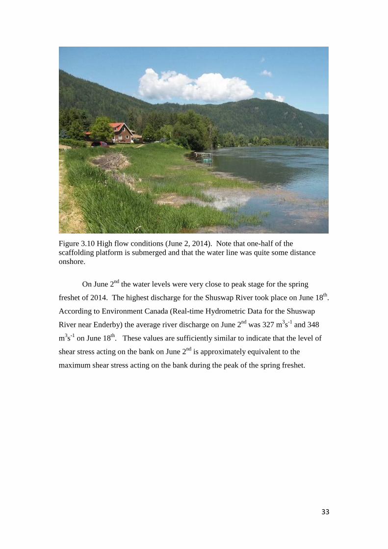
Figure 3.10 High flow conditions (June 2, 2014). Note that one-half of the scaffolding platform is submerged and that the water line was quite some distance onshore.

On June 2nd the water levels were very close to peak stage for the spring

freshet of 2014. The highest discharge for the Shuswap River took place on June 18th.

According to Environment Canada (Real-time Hydrometric Data for the Shuswap

River near Enderby) the average river discharge on June 2nd was 327 m3s-1 and 348

m3s-1 on June 18th. These values are sufficiently similar to indicate that the level of

shear stress acting on the bank on June 2nd is approximately equivalent to the

maximum shear stress acting on the bank during the peak of the spring freshet.

34

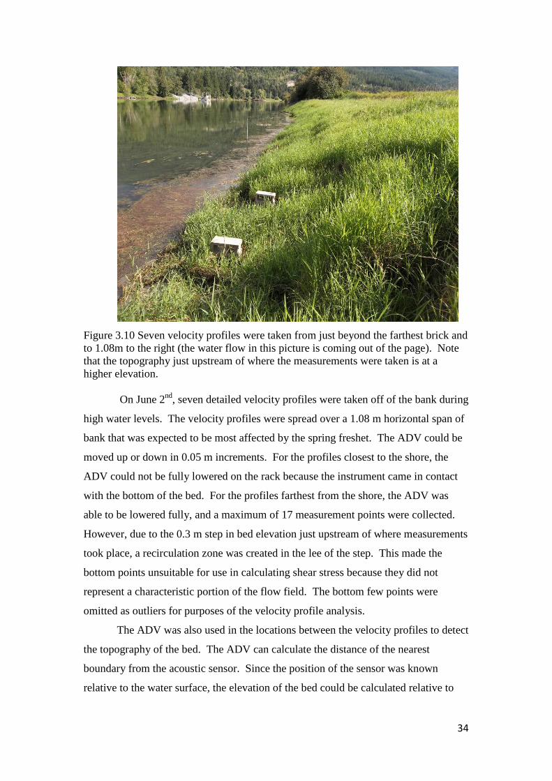
Figure 3.10 Seven velocity profiles were taken from just beyond the farthest brick and to 1.08m to the right (the water flow in this picture is coming out of the page). Note that the topography just upstream of where the measurements were taken is at a higher elevation.

On June 2nd, seven detailed velocity profiles were taken off of the bank during

high water levels. The velocity profiles were spread over a 1.08 m horizontal span of

bank that was expected to be most affected by the spring freshet. The ADV could be

moved up or down in 0.05 m increments. For the profiles closest to the shore, the

ADV could not be fully lowered on the rack because the instrument came in contact

with the bottom of the bed. For the profiles farthest from the shore, the ADV was

able to be lowered fully, and a maximum of 17 measurement points were collected.

However, due to the 0.3 m step in bed elevation just upstream of where measurements

took place, a recirculation zone was created in the lee of the step. This made the

bottom points unsuitable for use in calculating shear stress because they did not

represent a characteristic portion of the flow field. The bottom few points were

omitted as outliers for purposes of the velocity profile analysis.

The ADV was also used in the locations between the velocity profiles to detect

the topography of the bed. The ADV can calculate the distance of the nearest

boundary from the acoustic sensor. Since the position of the sensor was known

relative to the water surface, the elevation of the bed could be calculated relative to

35

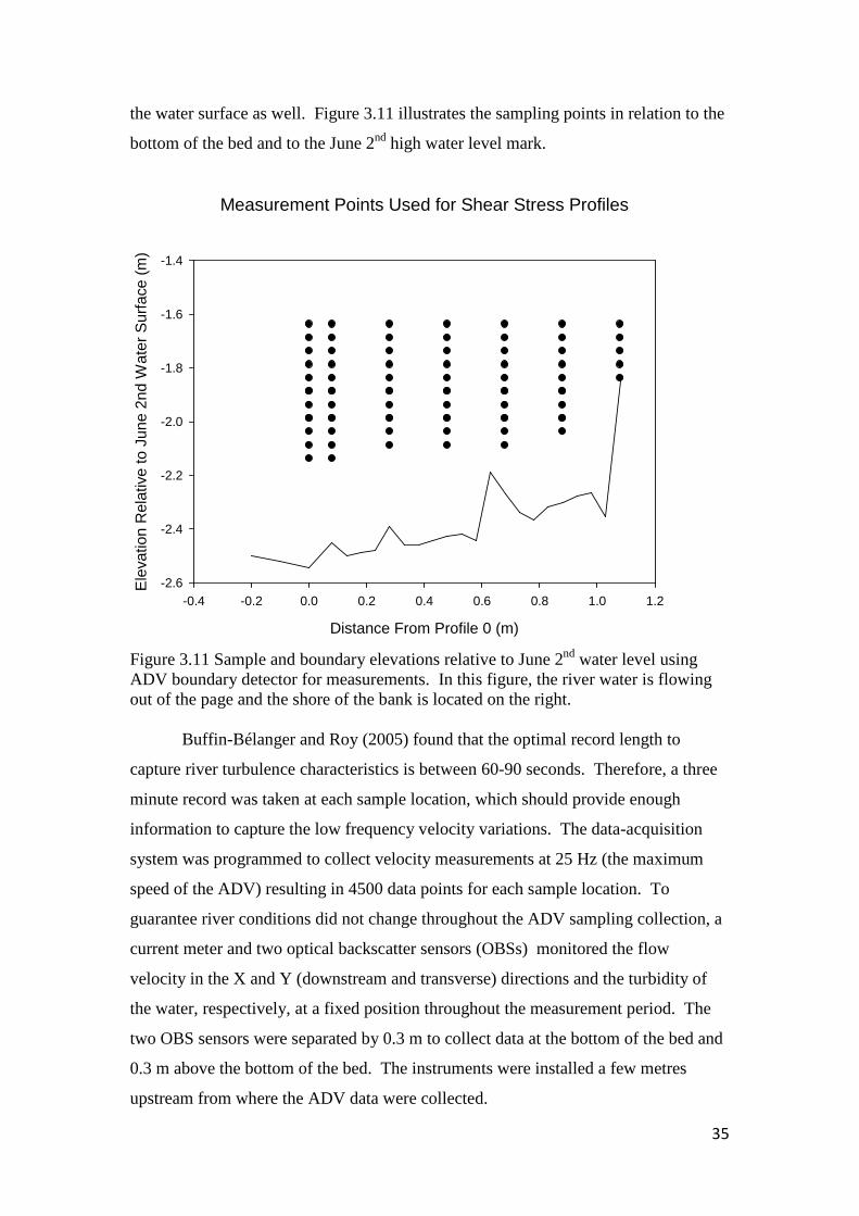
the water surface as well. Figure 3.11 illustrates the sampling points in relation to the

bottom of the bed and to the June 2nd high water level mark.

Measurement Points Used for Shear Stress Profiles

Distance From Profile 0 (m)

-0.4 -0.2 0.0 0.2 0.4 0.6 0.8 1.0 1.2

Ele

vatio

n R

elat

ive

to J

une

2nd

Wat

er S

urfa

ce (m

)

-2.6

-2.4

-2.2

-2.0

-1.8

-1.6

-1.4

Figure 3.11 Sample and boundary elevations relative to June 2nd water level using ADV boundary detector for measurements. In this figure, the river water is flowing out of the page and the shore of the bank is located on the right.

Buffin-Bélanger and Roy (2005) found that the optimal record length to

capture river turbulence characteristics is between 60-90 seconds. Therefore, a three

minute record was taken at each sample location, which should provide enough

information to capture the low frequency velocity variations. The data-acquisition

system was programmed to collect velocity measurements at 25 Hz (the maximum

speed of the ADV) resulting in 4500 data points for each sample location. To

guarantee river conditions did not change throughout the ADV sampling collection, a

current meter and two optical backscatter sensors (OBSs) monitored the flow

velocity in the X and Y (downstream and transverse) directions and the turbidity of

the water, respectively, at a fixed position throughout the measurement period. The

two OBS sensors were separated by 0.3 m to collect data at the bottom of the bed and

0.3 m above the bottom of the bed. The instruments were installed a few metres

upstream from where the ADV data were collected.

36

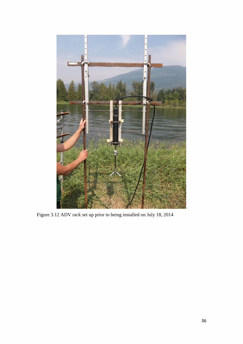
Figure 3.12 ADV rack set up prior to being installed on July 18, 2014

37

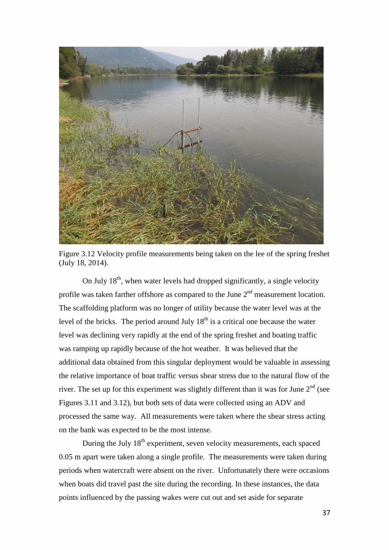
Figure 3.12 Velocity profile measurements being taken on the lee of the spring freshet (July 18, 2014).

On July 18th, when water levels had dropped significantly, a single velocity

profile was taken farther offshore as compared to the June 2nd measurement location.

The scaffolding platform was no longer of utility because the water level was at the

level of the bricks. The period around July 18th is a critical one because the water

level was declining very rapidly at the end of the spring freshet and boating traffic

was ramping up rapidly because of the hot weather. It was believed that the

additional data obtained from this singular deployment would be valuable in assessing

the relative importance of boat traffic versus shear stress due to the natural flow of the

river. The set up for this experiment was slightly different than it was for June 2nd (see

Figures 3.11 and 3.12), but both sets of data were collected using an ADV and

processed the same way. All measurements were taken where the shear stress acting

on the bank was expected to be the most intense.

During the July 18th experiment, seven velocity measurements, each spaced

0.05 m apart were taken along a single profile. The measurements were taken during

periods when watercraft were absent on the river. Unfortunately there were occasions

when boats did travel past the site during the recording. In these instances, the data

points influenced by the passing wakes were cut out and set aside for separate

38

analysis. A sampling duration of three minutes was used and data were collected at

25 Hz, as before.

All ADV data were analyzed using a program called WinADV, provided by

SonTek. Each file associated with a single sampling run had 4500 data points. The

raw data were filtered to remove any measurements that had a signal-to-noise ratio

smaller than 5 or a correlation under 70. Less than 0.53% of the original data were

filtered out using these criteria, which shows that the data are of very high quality.

The filtered data were exported into an Excel format for manipulation, and eventually

imported into Sigma Plot for graphing.

Velocity profiles are necessary to solve for shear stress (Equations 2 and 3)

and to understand the flow characteristics of the river. Various components of the

velocity field can be used in such an analysis, but for our purposes it was decided that

flow speed (Suvw) would be the truest representation of the flow field. Flow speed is

the magnitude of three-dimensional flow vector, and it can be calculated as follows:

Suvw = √(u2 + v2 + w2) (10)

where u, v and w are the instantaneous velocities in the x, y and z directions,

respectively. In order to produce a speed profile, the mean (Suvw������) was calculated for

every sample file by summing all the instantaneous Suvw values and dividing by n, the

number of samples in the file (typically 4500). The speed profile is generated by

comparing the mean speed against the natural logarithm of the distance from the

bottom measurement (Equation 2). The slope of line is proportional to the shear stress

acting on the bed (Equation 3). The bed shear stress values for each of the seven

profiles on June 2nd and the single profile collected on July 18th were calculated using

this technique.

Shear stress was also calculated using a Reynolds Stress method (Equation 6).

In this instance, the flow speed along the horizontal (X-Y) plane was used (Equation

5), which is referred to as Suv. The Reynolds Stress was then calculated using the

following equations:

Suv���� = 1/n ∑ Suv (11)

S'uv = Suv - Suv���� (12)

39

τSw = - ρ Suv ′ w′��������� (13)

for which any term with an overbar refers to an average (mean) quantity, a prime (')

indicates a fluctuating component, and an unprimed quantity refers to the

instantaneous variable in the time series. For Equation 13, τSw is the shear stress and ρ

is the density of the fluid. Note that the averaging is done on the cross-multiplied

terms, not on the separate terms prior to averaging. In statistics, terms such as these

are equivalent to cross-correlations, and this indicates that the Reynolds Stress is a

measure of the degree to which the fluctuating components in the velocity field (in the

downstream and vertical directions) are correlated. Large correlations are expected

for strongly sheared flows such as those close to fixed boundaries.

The Reynolds Stress method provides a shear stress value for each

measurement location rather than an overall average stress on the bank. However, a

shear stress profile can be plotted and extrapolated to the surface to provide an

estimate of shear stress on the bed or bank. As stated earlier, there was a recirculation

zone at the base of our velocity profiles, so the lowermost points in the profiles were

removed during filtering. The upper points in the profile were used to estimate the

bed shear stress.

3.5 Topographic Surveying

A number of topographic surveys were conducted on the Bruns property

between May 27, 2014 and August 2, 2014, including detailed surveys of the five

erosion-pin profile lines and of the topography immediately upstream of the

scaffolding. The profile data from Laderoute and Bauer (2013) were placed in a

common reference framework and combined with the 2014 data relative to a standard

high water stage (June 2, 2014). In addition, a detailed survey of a 6 m by 5 m grid

was undertaken to characterise the topography of the river bank. The hope had been

to survey this grid prior to the arrival of the spring freshet and then to re-occupy the

site after the freshet to assess bank change. However only a portion of the grid was

completed on April 27, 2014 and soon thereafter the water stage rose to a level that

precluded access to the grid. The remainder of the grid was completed between July

9 and July 25, 2014 as the water levels declined, and the data were used to produce a

40

Digital Elevation Model. Corner pins were left in the field so that the grid can be re-

occupied in future years.

On June 10, 2014 water surface slope was measured in order to drive

calculations such as tractive force. Unfortunately because of backwater effects from

the lake at this downstream site (close to the mouth of the river), the measured water

surface slope was essentially zero, taking into account measurement uncertainty. In

fact, a regression line through the water surface elevation data taken along the 385 m

reach suggests that the water surface slope was actually negative with a mean change

of -0.01 mm.

41

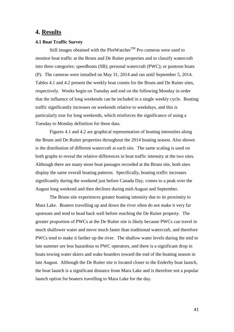
4. Results 4.1 Boat Traffic Survey

Still images obtained with the PlotWatcherTM Pro cameras were used to

monitor boat traffic at the Bruns and De Ruiter properties and to classify watercraft

into three categories: speedboats (SB); personal watercraft (PWC); or pontoon boats

(P). The cameras were installed on May 31, 2014 and ran until September 5, 2014.

Tables 4.1 and 4.2 present the weekly boat counts for the Bruns and De Ruiter sites,

respectively. Weeks begin on Tuesday and end on the following Monday in order

that the influence of long weekends can be included in a single weekly cycle. Boating

traffic significantly increases on weekends relative to weekdays, and this is

particularly true for long weekends, which reinforces the significance of using a

Tuesday to Monday definition for these data.

Figures 4.1 and 4.2 are graphical representation of boating intensities along

the Bruns and De Ruiter properties throughout the 2014 boating season. Also shown

is the distribution of different watercraft at each site. The same scaling is used on

both graphs to reveal the relative differences in boat traffic intensity at the two sites.

Although there are many more boat passages recorded at the Bruns site, both sites

display the same overall boating patterns. Specifically, boating traffic increases

significantly during the weekend just before Canada Day, comes to a peak over the

August long weekend and then declines during mid-August and September.

The Bruns site experiences greater boating intensity due to its proximity to

Mara Lake. Boaters travelling up and down the river often do not make it very far

upstream and tend to head back well before reaching the De Ruiter property. The

greater proportion of PWCs at the De Ruiter site is likely because PWCs can travel in

much shallower water and move much faster than traditional watercraft, and therefore

PWCs tend to make it farther up the river. The shallow water levels during the mid to

late summer are less hazardous to PWC operators, and there is a significant drop in

boats towing water skiers and wake boarders toward the end of the boating season in

late August. Although the De Ruiter site is located closer to the Enderby boat launch,

the boat launch is a significant distance from Mara Lake and is therefore not a popular

launch option for boaters travelling to Mara Lake for the day.

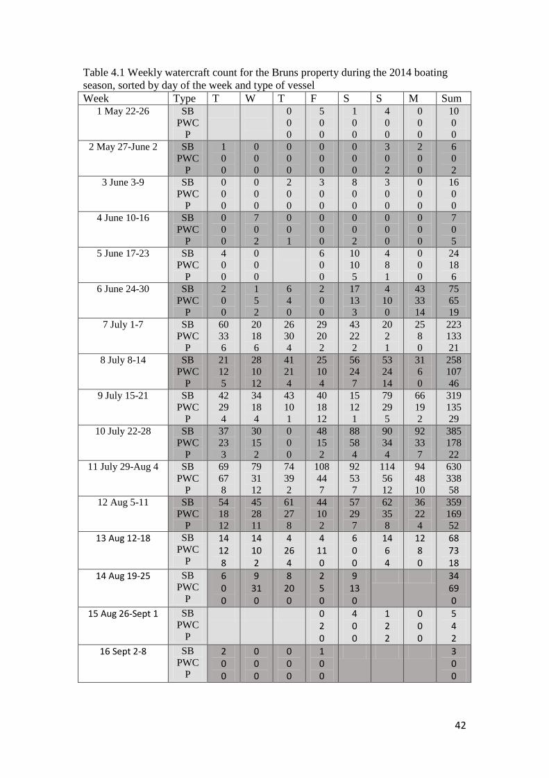
42

Table 4.1 Weekly watercraft count for the Bruns property during the 2014 boating season, sorted by day of the week and type of vessel Week Type T W T F S S M Sum

1 May 22-26 SB PWC

P

0 0 0

5 0 0

1 0 0

4 0 0

0 0 0

10 0 0

2 May 27-June 2 SB PWC

P

1 0 0

0 0 0

0 0 0

0 0 0

0 0 0

3 0 2

2 0 0

6 0 2

3 June 3-9 SB PWC

P

0 0 0

0 0 0

2 0 0

3 0 0

8 0 0

3 0 0

0 0 0

16 0 0

4 June 10-16 SB PWC

P

0 0 0

7 0 2

0 0 1

0 0 0

0 0 2

0 0 0

0 0 0

7 0 5

5 June 17-23 SB PWC

P

4 0 0

0 0 0

6 0 0

10 10 5

4 8 1

0 0 0

24 18 6

6 June 24-30 SB PWC

P

2 0 0

1 5 2

6 4 0

2 0 0

17 13 3

4 10 0

43 33 14

75 65 19

7 July 1-7 SB PWC

P

60 33 6

20 18 6

26 30 4

29 20 2

43 22 2

20 2 1

25 8 0

223 133 21

8 July 8-14 SB PWC

P

21 12 5

28 10 12

41 21 4

25 10 4

56 24 7

53 24 14

31 6 0

258 107 46

9 July 15-21 SB PWC

P

42 29 4

34 18 4

43 10 1

40 18 12

15 12 1

79 29 5

66 19 2

319 135 29

10 July 22-28 SB PWC

P

37 23 3

30 15 2

0 0 0

48 15 2

88 58 4

90 34 4

92 33 7

385 178 22

11 July 29-Aug 4 SB PWC

P

69 67 8

79 31 12

74 39 2

108 44 7

92 53 7

114 56 12

94 48 10

630 338 58

12 Aug 5-11 SB PWC

P

54 18 12

45 28 11

61 27 8

44 10 2

57 29 7

62 35 8

36 22 4

359 169 52

13 Aug 12-18 SB PWC

P

14 12 8

14 10 2

4 26 4

4 11 0

6 0 0

14 6 4

12 8 0

68 73 18

14 Aug 19-25 SB PWC

P

6 0 0

9 31 0

8 20 0

2 5 0

9 13 0

34 69 0

15 Aug 26-Sept 1 SB PWC

P

0 2 0

4 0 0

1 2 2

0 0 0

5 4 2

16 Sept 2-8 SB PWC

P

2 0 0

0 0 0

0 0 0

1 0 0

3 0 0

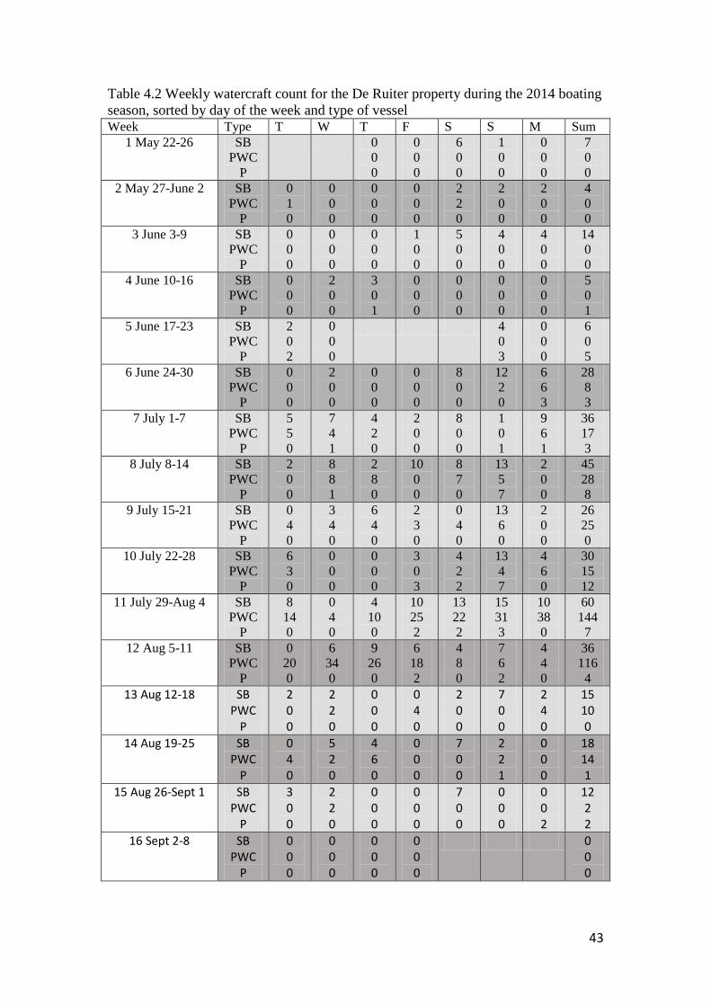
43

Table 4.2 Weekly watercraft count for the De Ruiter property during the 2014 boating season, sorted by day of the week and type of vessel Week Type T W T F S S M Sum

1 May 22-26 SB PWC

P

0 0 0

0 0 0

6 0 0

1 0 0

0 0 0

7 0 0

2 May 27-June 2 SB PWC

P

0 1 0

0 0 0

0 0 0

0 0 0

2 2 0

2 0 0

2 0 0

4 0 0

3 June 3-9 SB PWC

P

0 0 0

0 0 0

0 0 0

1 0 0

5 0 0

4 0 0

4 0 0

14 0 0

4 June 10-16 SB PWC

P

0 0 0

2 0 0

3 0 1

0 0 0

0 0 0

0 0 0

0 0 0

5 0 1

5 June 17-23 SB PWC

P

2 0 2

0 0 0

4 0 3

0 0 0

6 0 5

6 June 24-30 SB PWC

P

0 0 0

2 0 0

0 0 0

0 0 0

8 0 0

12 2 0

6 6 3

28 8 3

7 July 1-7 SB PWC

P

5 5 0

7 4 1

4 2 0

2 0 0

8 0 0

1 0 1

9 6 1

36 17 3

8 July 8-14 SB PWC

P

2 0 0

8 8 1

2 8 0

10 0 0

8 7 0

13 5 7

2 0 0

45 28 8

9 July 15-21 SB PWC

P

0 4 0

3 4 0

6 4 0

2 3 0

0 4 0

13 6 0

2 0 0

26 25 0

10 July 22-28 SB PWC

P

6 3 0

0 0 0

0 0 0

3 0 3

4 2 2

13 4 7

4 6 0

30 15 12

11 July 29-Aug 4 SB PWC

P

8 14 0

0 4 0

4 10 0

10 25 2

13 22 2

15 31 3

10 38 0

60 144

7 12 Aug 5-11 SB

PWC P

0 20 0

6 34 0

9 26 0

6 18 2

4 8 0

7 6 2

4 4 0

36 116

4 13 Aug 12-18 SB

PWC P

2 0 0

2 2 0

0 0 0

0 4 0

2 0 0

7 0 0

2 4 0

15 10 0

14 Aug 19-25 SB PWC

P

0 4 0

5 2 0

4 6 0

0 0 0

7 0 0

2 2 1

0 0 0

18 14 1

15 Aug 26-Sept 1 SB PWC

P

3 0 0

2 2 0

0 0 0

0 0 0

7 0 0

0 0 0

0 0 2

12 2 2

16 Sept 2-8 SB PWC

P

0 0 0

0 0 0

0 0 0

0 0 0

0 0 0

44

Figure 4.1 Weekly watercraft count by speedboats (SB), personal watercraft (PWC) and pontoon boats (P) at the Bruns property during the 2014 boating season.

Figure 4.2 Weekly watercraft count by speedboats (SB), personal watercraft (PWC) and pontoon boats (P) at the De Ruiter property during the 2014 boating season.

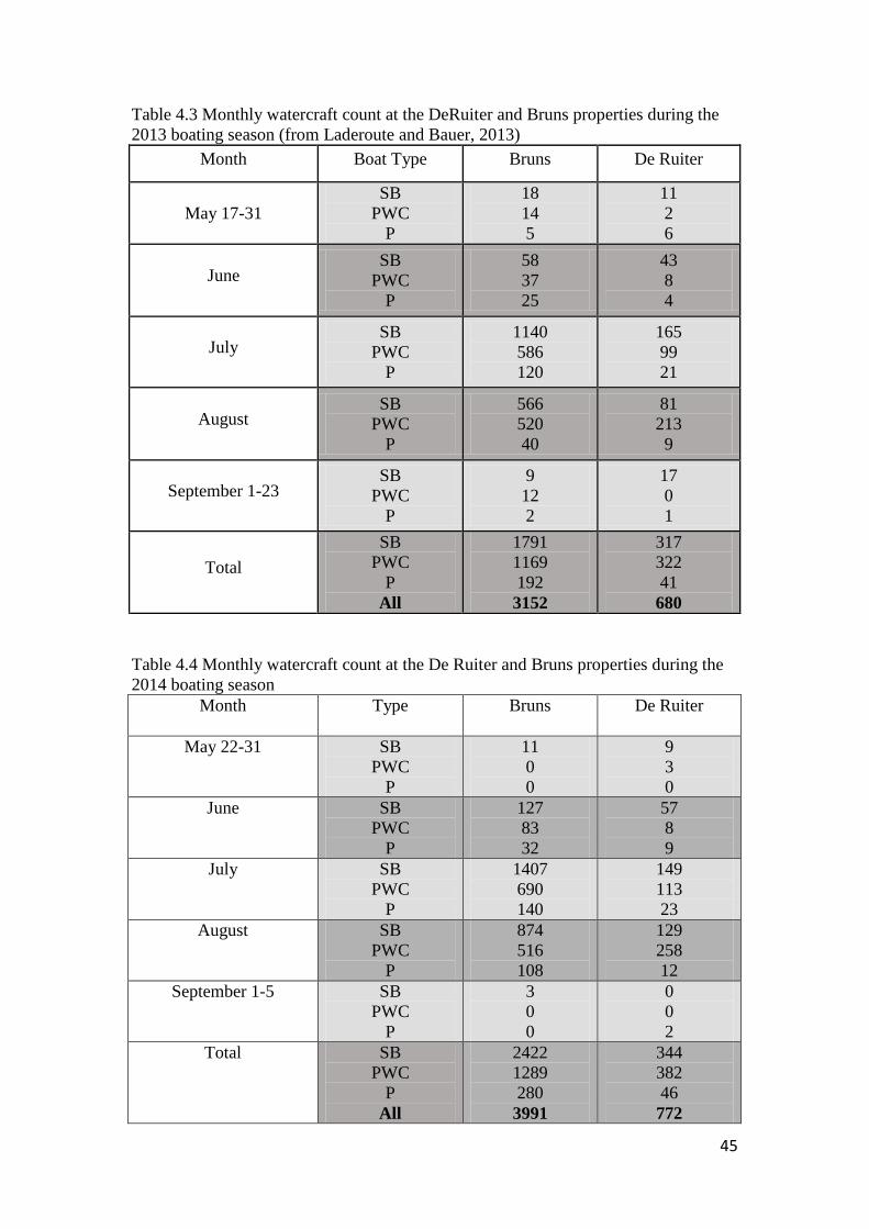
45

Table 4.3 Monthly watercraft count at the DeRuiter and Bruns properties during the 2013 boating season (from Laderoute and Bauer, 2013)

Month Boat Type Bruns De Ruiter

May 17-31 SB

PWC P

18 14 5

11 2 6

June SB

PWC P

58 37 25

43 8 4

July SB

PWC P

1140 586 120

165 99 21

August SB

PWC P

566 520 40

81 213 9

September 1-23 SB

PWC P

9 12 2

17 0 1

Total SB

PWC P

All

1791 1169 192 3152

317 322 41 680

Table 4.4 Monthly watercraft count at the De Ruiter and Bruns properties during the 2014 boating season

Month

Type Bruns De Ruiter

May 22-31 SB PWC

P

11 0 0

9 3 0

June SB PWC

P

127 83 32

57 8 9

July SB PWC

P

1407 690 140

149 113 23

August SB PWC

P

874 516 108

129 258 12

September 1-5 SB PWC

P

3 0 0

0 0 2

Total SB PWC

P All

2422 1289 280 3991

344 382 46 772

46

Tables 4.3 and 4.4 compare the monthly boat counts for the 2013 and 2014

boating season, respectively. As shown, despite the longer monitoring period

throughout the summer of 2013, the 2014 boating season experienced 839 and 92

more vessel passages at the Bruns and De Ruiter sites respectively. Although there is

not enough data to conclude any long term trends, it is clear that boating traffic will

vary from year to year. If bank erosion is linearly related to boat wakes then more

bank erosion is to be expected in 2014 compared to 2013.

4.2 Short-Term Water Velocity and Turbulence Monitoring

On June 2, 2014, seven velocity profiles were taken next to the river bank at

the Bruns property during a high flow period. These vertical profiles were named

Profile 0, Profile 1, Profile 3, Profile 5, Profile 7, Profile 9 and Profile 11 and spanned

a distance of 1.08 m perpendicular to the bank. Profile 0 was located farthest from

the bank (in deep water) and Profile 11 was closest to shore (in shallow water). The

original intent was to measure profiles at 0.05 m spacings in the horizontal, but this

proved to be too time consuming and the spacing too small leading to profile

redundancy. Profile 0 and Profile 1 were separated by 0.08 m and all other profiles

were separated by 0.1 m. The general layout of the profile lines relative to the bed

were shown in Figure 3.11, in the Methods chapter.

Figures 4.3 to 4.9 show the speed profiles for the seven vertical profiles taken

on the 1.08 m horizontal span of river bank. Each speed profile was generated using

the mean speed at each sample location during the three-minute sampling period

(Equation 10). Note that the bottom samples of each profile have been removed

because they were located in the recirculation zone at the base of the scaffolding

platform. These points had minimal or negative velocities, which skewed the profiles

unrealistically. The number of points removed depended on the height of the bed

immediately upstream of the profile, which varied from profile to profile. All profiles

except Profile 11 have at least 10 points in the profile, which makes for robust

regression analysis. Profile 11, which is closest to the bank, only has five points

because the profile was positioned immediately above the large bricks that supported

the scaffolding and the probe could not be lowered to greater depths.

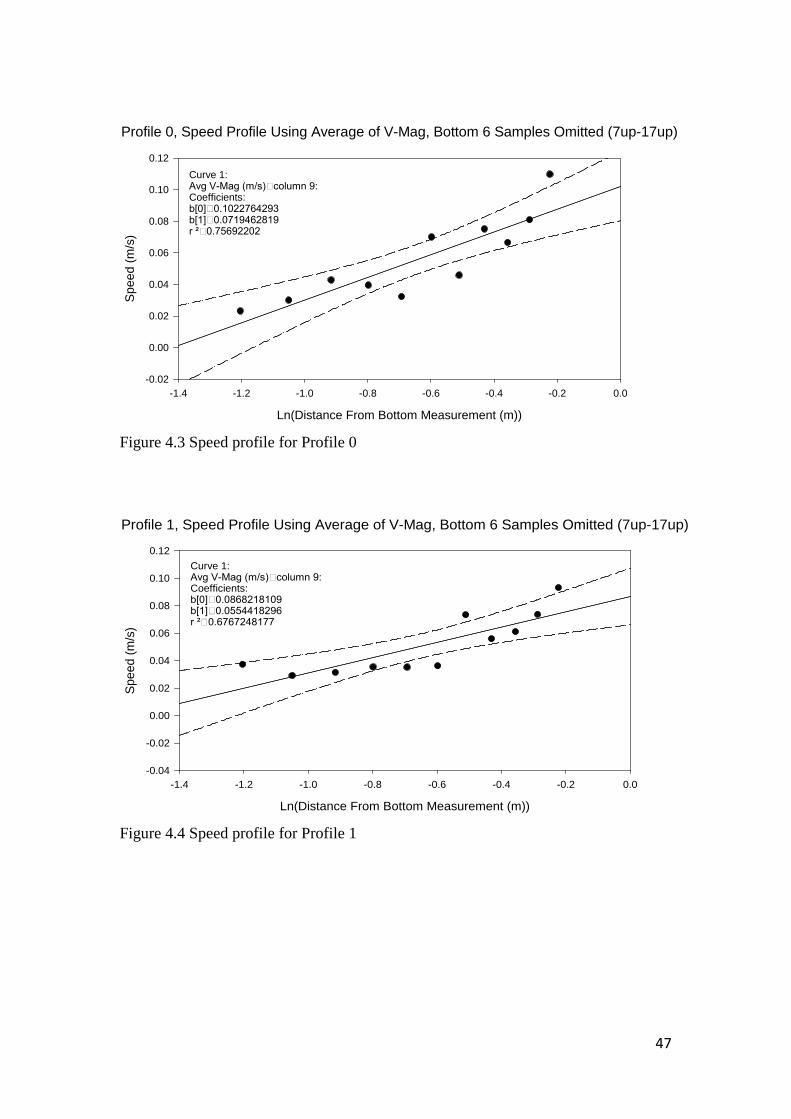
47

Figure 4.3 Speed profile for Profile 0

Figure 4.4 Speed profile for Profile 1

Profile 0, Speed Profile Using Average of V-Mag, Bottom 6 Samples Omitted (7up-17up)

Ln(Distance From Bottom Measurement (m))

-1.4 -1.2 -1.0 -0.8 -0.6 -0.4 -0.2 0.0

Spe

ed (m

/s)

-0.02

0.00

0.02

0.04

0.06

0.08

0.10

0.12Curve 1:Avg V-Mag (m/s)column 9:Coefficients:b[0]0.1022764293b[1]0.0719462819r ²0.75692202

Profile 1, Speed Profile Using Average of V-Mag, Bottom 6 Samples Omitted (7up-17up)

Ln(Distance From Bottom Measurement (m))

-1.4 -1.2 -1.0 -0.8 -0.6 -0.4 -0.2 0.0

Spee

d (m

/s)

-0.04

-0.02

0.00

0.02

0.04

0.06

0.08

0.10

0.12Curve 1:Avg V-Mag (m/s)column 9:Coefficients:b[0]0.0868218109b[1]0.0554418296r ²0.6767248177

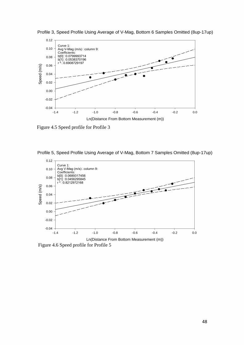
48

Figure 4.5 Speed profile for Profile 3

Figure 4.6 Speed profile for Profile 5

Profile 3, Speed Profile Using Average of V-Mag, Bottom 6 Samples Omitted (8up-17up)

Ln(Distance From Bottom Measurement (m))

-1.4 -1.2 -1.0 -0.8 -0.6 -0.4 -0.2 0.0

Spee

d (m

/s)

-0.04

-0.02

0.00

0.02

0.04

0.06

0.08

0.10

0.12

Curve 1:Avg V-Mag (m/s)column 9:Coefficients:b[0]0.0799993714b[1]0.0538370196r ²0.6908729197

Profile 5, Speed Profile Using Average of V-Mag, Bottom 7 Samples Omitted (8up-17up)

Ln(Distance From Bottom Measurement (m))

-1.4 -1.2 -1.0 -0.8 -0.6 -0.4 -0.2 0.0

Spee

d (m

/s)

-0.04

-0.02

0.00

0.02

0.04

0.06

0.08

0.10

0.12Curve 1:Avg V-Mag (m/s)column 9:Coefficients:b[0]0.0689317456b[1]0.0456295845r ²0.8212972168

49

Figure 4.7 Speed profile for Profile 7

Figure 4.8 Speed profile for Profile 8

Profile 7, Speed Profile Using Average of V-Mag, Bottom 3 Samples Omitted (8up-17up)

Ln(Distance From Bottom Measurement (m))

-1.4 -1.2 -1.0 -0.8 -0.6 -0.4 -0.2 0.0

Spee

d (m

/s)

-0.04

-0.02

0.00

0.02

0.04

0.06

0.08

0.10

0.12Curve 1:Avg V-Mag (m/s)column 9:Coefficients:b[0]0.0578699819b[1]0.037514161r ²0.6118735093

Profile 9, Speed Profile Using Average of V-Mag, Bottom 5 Samples Omitted (9up-17up)

Ln(Distance From Bottom Measurement (m))

-1.4 -1.2 -1.0 -0.8 -0.6 -0.4 -0.2 0.0

Spee

d (m

/s)

-0.04

-0.02

0.00

0.02

0.04

0.06

0.08

0.10

0.12Curve 1:Avg V-Mag (m/s)column 9:Coefficients:b[0]0.0542036308b[1]0.0350808881r ²0.5419838606

50

Figure 4.9 Speed profile for Profile 11

From these speed profiles, u* was derived from the regression coefficients

because u* is equal to the slope multiplied by the von Karman constant (equal to

approximately 0.4). The value of shear stress acting on the bed was then determined

using Equation 3. The calculated boundary shear stress values for each profile using

the Law of the Wall method are given in Table 4.5.

Table 4.5 Boundary shear stress values obtained using the Law of the Wall method and the Reynolds Stress method Boundary Shear Stress Calculated

Using Avg. V-Mag (N m-2) Average of Upper 5 Boundary Shear Stress Using Suv’w’ as Reynolds Stress (N m-2)

Profile 0 0.827 0.423

Profile 1 0.491 0.308

Profile 3 0.463 0.307

Profile 5 0.332 0.176

Profile 7 0.225 0.186

Profile 9 0.196 0.074

Profile 11 0.498 0.062

Profile 11, Speed Profile Using Average of V-Mag, No Samples Omitted (13up-17up)

Ln(Distance From Bottom Measurement (m))

-1.4 -1.2 -1.0 -0.8 -0.6 -0.4 -0.2 0.0

Spee

d (m

/s)

-0.04

-0.02

0.00

0.02

0.04

0.06

0.08

0.10

0.12

Avg V-Mag (m/s)column 9:Coefficients:b[0]0.0538919953b[1]0.0558180686r ²0.8089648625

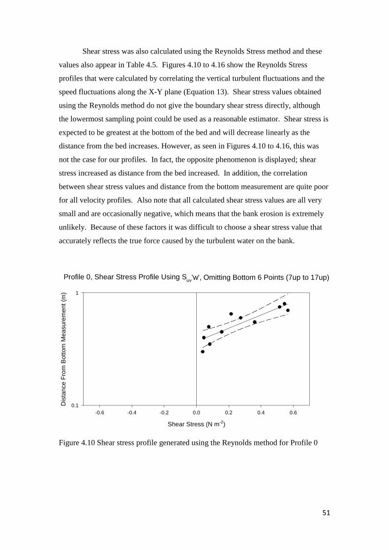
51

Shear stress was also calculated using the Reynolds Stress method and these

values also appear in Table 4.5. Figures 4.10 to 4.16 show the Reynolds Stress

profiles that were calculated by correlating the vertical turbulent fluctuations and the

speed fluctuations along the X-Y plane (Equation 13). Shear stress values obtained

using the Reynolds method do not give the boundary shear stress directly, although

the lowermost sampling point could be used as a reasonable estimator. Shear stress is

expected to be greatest at the bottom of the bed and will decrease linearly as the

distance from the bed increases. However, as seen in Figures 4.10 to 4.16, this was

not the case for our profiles. In fact, the opposite phenomenon is displayed; shear

stress increased as distance from the bed increased. In addition, the correlation

between shear stress values and distance from the bottom measurement are quite poor

for all velocity profiles. Also note that all calculated shear stress values are all very

small and are occasionally negative, which means that the bank erosion is extremely

unlikely. Because of these factors it was difficult to choose a shear stress value that

accurately reflects the true force caused by the turbulent water on the bank.

Figure 4.10 Shear stress profile generated using the Reynolds method for Profile 0

Profile 0, Shear Stress Profile Using Suv'w', Omitting Bottom 6 Points (7up to 17up)

Shear Stress (N m-2)

-0.6 -0.4 -0.2 0.0 0.2 0.4 0.6

Dis

tanc

e Fr

om B

otto

m M

easu

rem

ent (

m)

0.1

1

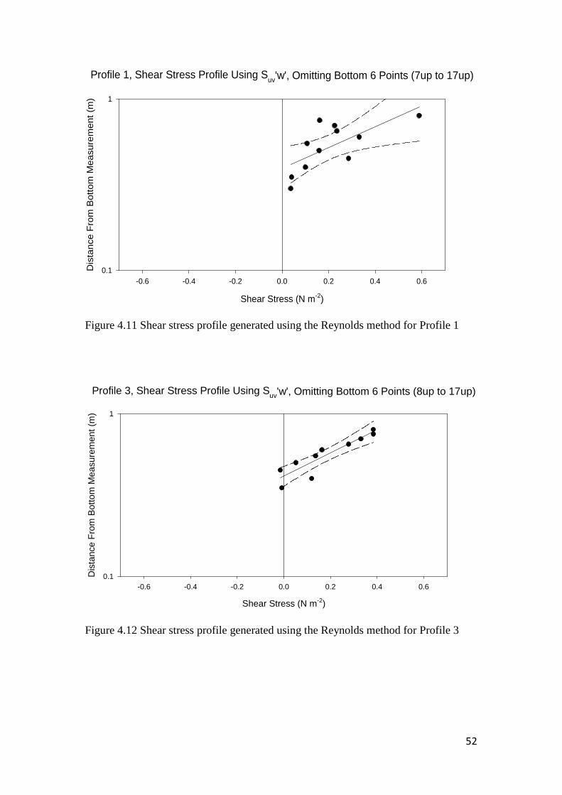
52

Figure 4.11 Shear stress profile generated using the Reynolds method for Profile 1

Figure 4.12 Shear stress profile generated using the Reynolds method for Profile 3

Profile 3, Shear Stress Profile Using Suv'w', Omitting Bottom 6 Points (8up to 17up)

Shear Stress (N m-2)

-0.6 -0.4 -0.2 0.0 0.2 0.4 0.6

Dis

tanc

e Fr

om B

otto

m M

easu

rem

ent (

m)

0.1

1

Profile 1, Shear Stress Profile Using Suv'w', Omitting Bottom 6 Points (7up to 17up)

Shear Stress (N m-2)

-0.6 -0.4 -0.2 0.0 0.2 0.4 0.6

Dis

tanc

e Fr

om B

otto

m M

easu

rem

ent (

m)

0.1

1

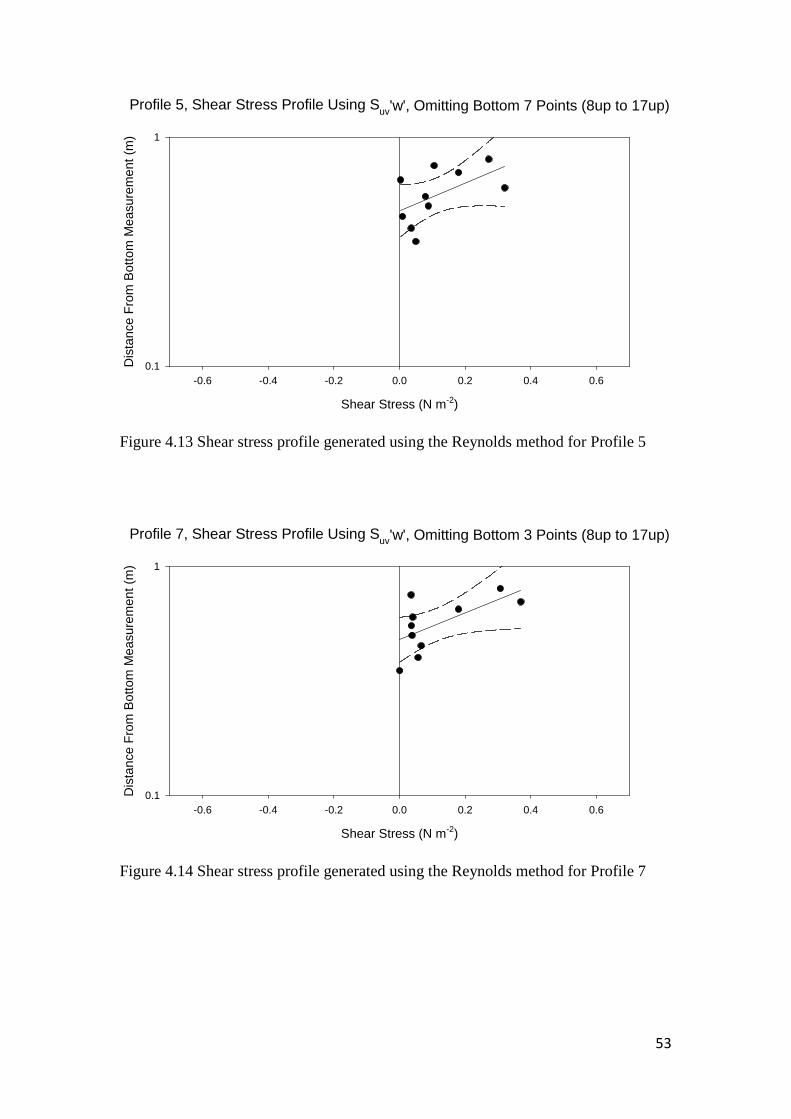
53

Figure 4.13 Shear stress profile generated using the Reynolds method for Profile 5

Figure 4.14 Shear stress profile generated using the Reynolds method for Profile 7

Profile 5, Shear Stress Profile Using Suv'w', Omitting Bottom 7 Points (8up to 17up)

Shear Stress (N m-2)

-0.6 -0.4 -0.2 0.0 0.2 0.4 0.6

Dis

tanc

e Fr

om B

otto

m M

easu

rem

ent (

m)

0.1

1

Profile 7, Shear Stress Profile Using Suv'w', Omitting Bottom 3 Points (8up to 17up)

Shear Stress (N m-2)

-0.6 -0.4 -0.2 0.0 0.2 0.4 0.6

Dis

tanc

e Fr

om B

otto

m M

easu

rem

ent (

m)

0.1

1

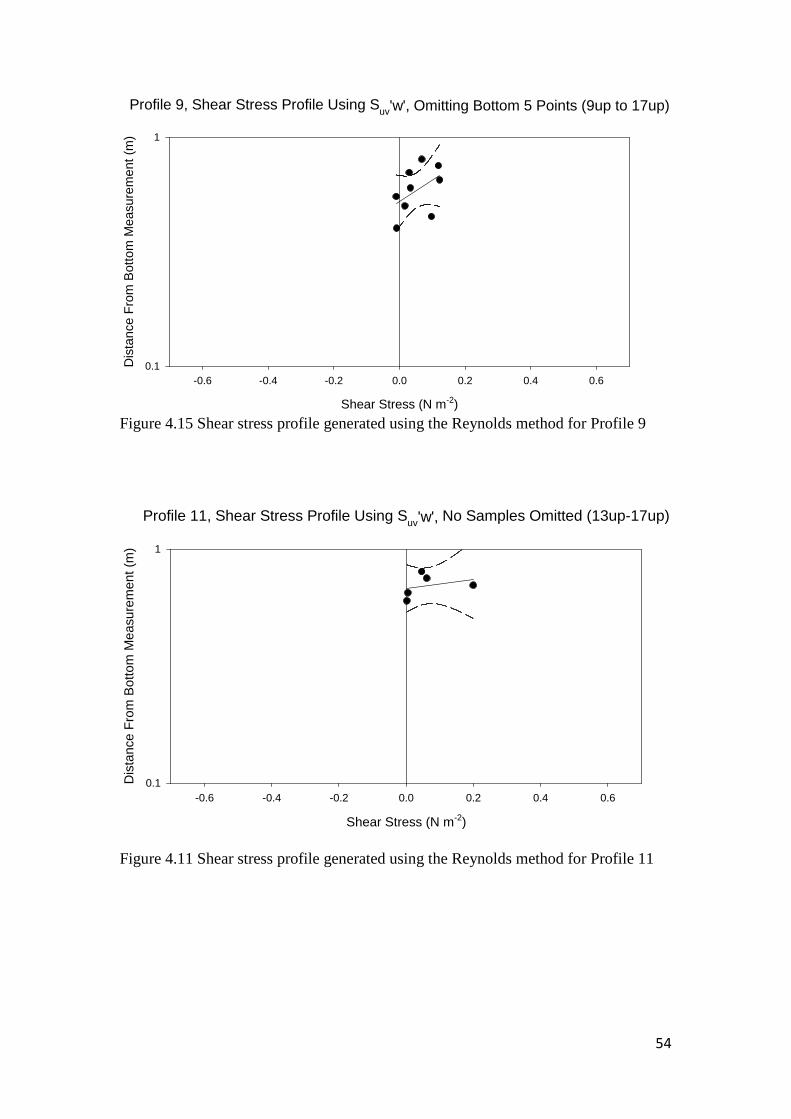
54

Figure 4.15 Shear stress profile generated using the Reynolds method for Profile 9

Figure 4.11 Shear stress profile generated using the Reynolds method for Profile 11

Profile 9, Shear Stress Profile Using Suv'w', Omitting Bottom 5 Points (9up to 17up)

Shear Stress (N m-2)

-0.6 -0.4 -0.2 0.0 0.2 0.4 0.6

Dis

tanc

e Fr

om B

otto

m M

easu

rem

ent (

m)

0.1

1

Profile 11, Shear Stress Profile Using Suv'w', No Samples Omitted (13up-17up)

Shear Stress (N m-2)

-0.6 -0.4 -0.2 0.0 0.2 0.4 0.6

Dis

tanc

e Fr

om B

otto

m M

easu

rem

ent (

m)

0.1

1

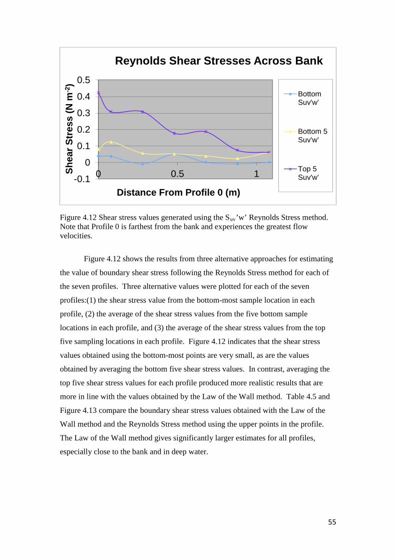
55

Figure 4.12 Shear stress values generated using the Suv’w’ Reynolds Stress method. Note that Profile 0 is farthest from the bank and experiences the greatest flow velocities.

Figure 4.12 shows the results from three alternative approaches for estimating

the value of boundary shear stress following the Reynolds Stress method for each of

the seven profiles. Three alternative values were plotted for each of the seven

profiles:(1) the shear stress value from the bottom-most sample location in each

profile, (2) the average of the shear stress values from the five bottom sample

locations in each profile, and (3) the average of the shear stress values from the top

five sampling locations in each profile. Figure 4.12 indicates that the shear stress

values obtained using the bottom-most points are very small, as are the values

obtained by averaging the bottom five shear stress values. In contrast, averaging the

top five shear stress values for each profile produced more realistic results that are

more in line with the values obtained by the Law of the Wall method. Table 4.5 and

Figure 4.13 compare the boundary shear stress values obtained with the Law of the

Wall method and the Reynolds Stress method using the upper points in the profile.

The Law of the Wall method gives significantly larger estimates for all profiles,

especially close to the bank and in deep water.

-0.1

0

0.1

0.2

0.3

0.4

0.5

0 0.5 1Shea

r Str

ess

(N m

-2)

Distance From Profile 0 (m)

Reynolds Shear Stresses Across Bank

BottomSuv'w'

Bottom 5Suv'w'

Top 5Suv'w'

56

Figure 4.13 Shear Stress values obtained from 7 profile measurements along the river bank at the Lower Shuwap River. Profile 0 is farthest from the bank in deepest water.

Although there is a significant difference between bottom shear stress values

calculated by the two methods, the trends are very similar. Specifically, the shear

stress is at its maximum for the farthest offshore profile (in deepest water) and

gradually decreases toward the bank. The single exception to this trend is the shear

stress estimate from the Law of the Wall for Profile 11, which is much larger than the

other estimates. The likely explanation for this is that the vertical speed profile is not

robust (see Figure 4.9) because it only has five points that are relatively high in the

flow domain. The other aspect of these shear stress values that is of note is that the

magnitudes are very small in comparison to what might be expected for near-bottom

stresses in the middle of a river of this size (typically 3 Nm-2 or greater). The largest

boundary shear stress value was obtained for Profile 0 using the Law of the Wall

method, and it was only 0.83 Nm-2. Examination of the Shields diagram (Figure 2.10)

shows that these small values are insufficient to promote any sort of erosion.

On July 18, 2014, another single velocity profile was taken using a different

deployment scheme farther offshore than the June 2 measurements. The water level

(and discharge) was greatly reduced, and the reason for measuring this profile was to

draw a comparison with the profiles during the height of the spring freshet. Seven

sampling points were taken along the vertical profile, starting close to the bottom and

increasing at 0.05 m intervals to reach an elevation of about 0.3 m above the bed. The

majority of samples were collected at 25 Hz for 180 seconds. However, due to boats

00.10.20.30.40.50.60.70.80.9

0 0.2 0.4 0.6 0.8 1 1.2

Shea

r Str

ess

(Nm

-2)

Distance From Profile 0 (m)

Bottom Shear Stress Values Across Bank

Avg V-Mag

Top 5Suv'w'

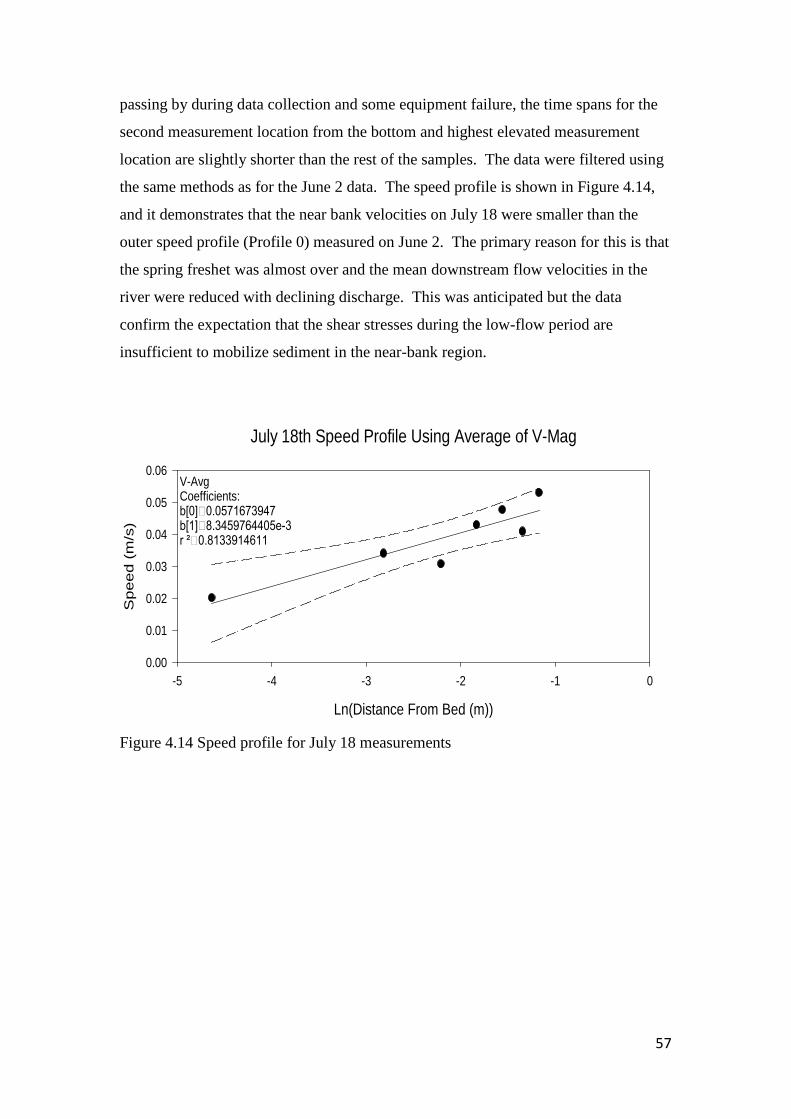
57

passing by during data collection and some equipment failure, the time spans for the

second measurement location from the bottom and highest elevated measurement

location are slightly shorter than the rest of the samples. The data were filtered using

the same methods as for the June 2 data. The speed profile is shown in Figure 4.14,

and it demonstrates that the near bank velocities on July 18 were smaller than the

outer speed profile (Profile 0) measured on June 2. The primary reason for this is that

the spring freshet was almost over and the mean downstream flow velocities in the

river were reduced with declining discharge. This was anticipated but the data

confirm the expectation that the shear stresses during the low-flow period are

insufficient to mobilize sediment in the near-bank region.

Figure 4.14 Speed profile for July 18 measurements

July 18th Speed Profile Using Average of V-Mag

Ln(Distance From Bed (m))

-5 -4 -3 -2 -1 0

Sp

ee

d (

m/s

)

0.00

0.01

0.02

0.03

0.04

0.05

0.06

V-AvgCoefficients:b[0]0.0571673947b[1]8.3459764405e-3r ²0.8133914611

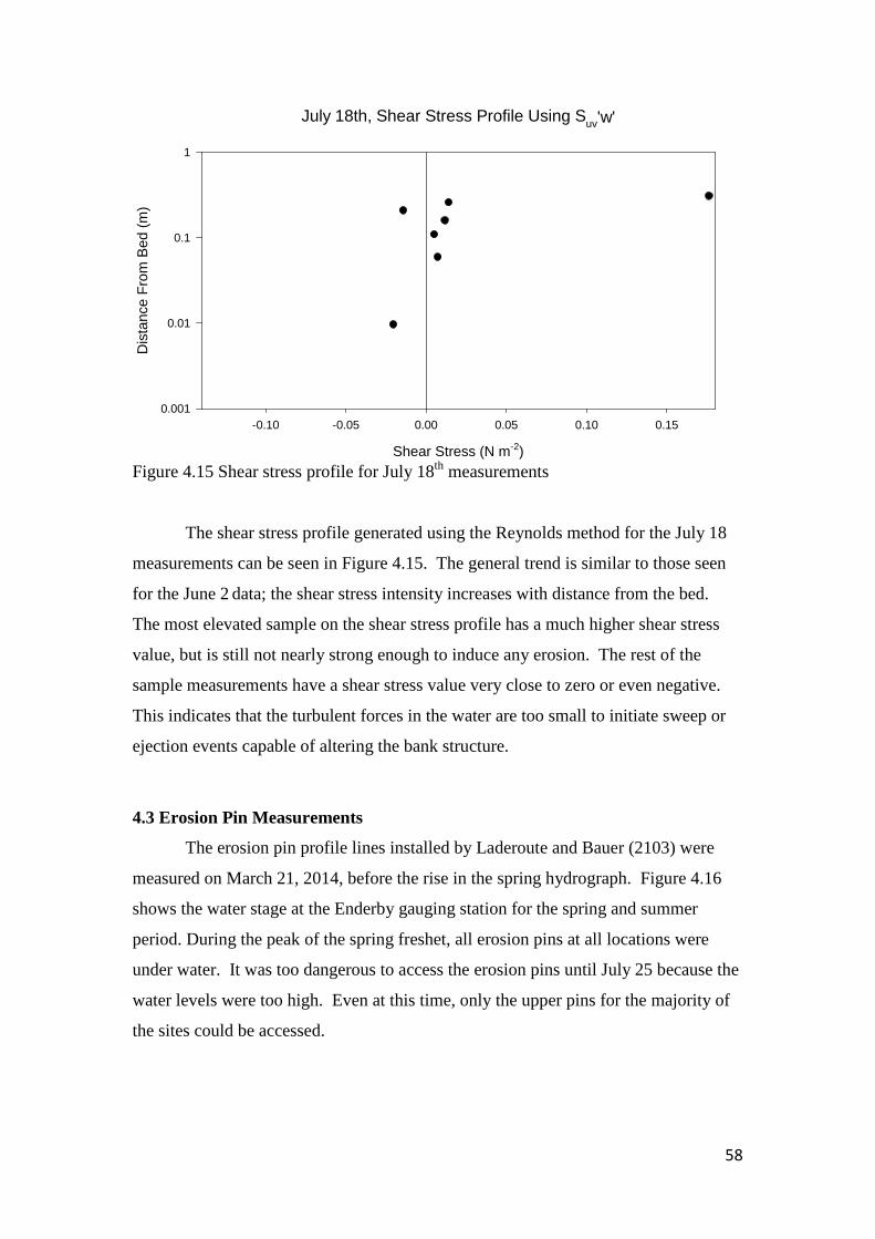
58

Figure 4.15 Shear stress profile for July 18th measurements

The shear stress profile generated using the Reynolds method for the July 18

measurements can be seen in Figure 4.15. The general trend is similar to those seen

for the June 2 data; the shear stress intensity increases with distance from the bed.

The most elevated sample on the shear stress profile has a much higher shear stress

value, but is still not nearly strong enough to induce any erosion. The rest of the

sample measurements have a shear stress value very close to zero or even negative.

This indicates that the turbulent forces in the water are too small to initiate sweep or

ejection events capable of altering the bank structure.

4.3 Erosion Pin Measurements

The erosion pin profile lines installed by Laderoute and Bauer (2103) were

measured on March 21, 2014, before the rise in the spring hydrograph. Figure 4.16

shows the water stage at the Enderby gauging station for the spring and summer

period. During the peak of the spring freshet, all erosion pins at all locations were

under water. It was too dangerous to access the erosion pins until July 25 because the

water levels were too high. Even at this time, only the upper pins for the majority of

the sites could be accessed.

July 18th, Shear Stress Profile Using Suv'w'

Shear Stress (N m-2)

-0.10 -0.05 0.00 0.05 0.10 0.15

Dis

tanc

e Fr

om B

ed (m

)

0.001

0.01

0.1

1

59

Figure 4.16 Water level recorded for the Shuswap River at Enderby during the summer of 2014 (Environment Canada Water Office, 2014)

Figure 4.17 Water level recorded for the Shuswap River at Enderby during the summer of 2013 (Environment Canada Water Office, 2014)

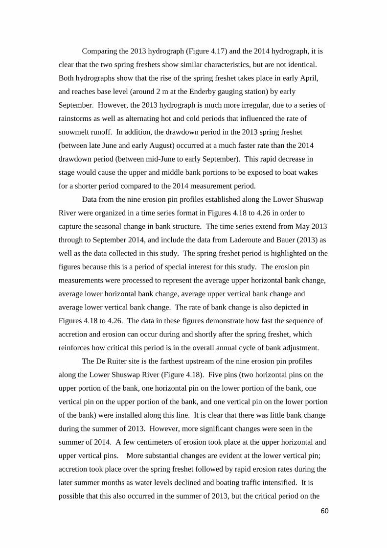
60

Comparing the 2013 hydrograph (Figure 4.17) and the 2014 hydrograph, it is

clear that the two spring freshets show similar characteristics, but are not identical.

Both hydrographs show that the rise of the spring freshet takes place in early April,

and reaches base level (around 2 m at the Enderby gauging station) by early

September. However, the 2013 hydrograph is much more irregular, due to a series of

rainstorms as well as alternating hot and cold periods that influenced the rate of

snowmelt runoff. In addition, the drawdown period in the 2013 spring freshet

(between late June and early August) occurred at a much faster rate than the 2014

drawdown period (between mid-June to early September). This rapid decrease in

stage would cause the upper and middle bank portions to be exposed to boat wakes

for a shorter period compared to the 2014 measurement period.

Data from the nine erosion pin profiles established along the Lower Shuswap

River were organized in a time series format in Figures 4.18 to 4.26 in order to

capture the seasonal change in bank structure. The time series extend from May 2013

through to September 2014, and include the data from Laderoute and Bauer (2013) as

well as the data collected in this study. The spring freshet period is highlighted on the

figures because this is a period of special interest for this study. The erosion pin

measurements were processed to represent the average upper horizontal bank change,

average lower horizontal bank change, average upper vertical bank change and

average lower vertical bank change. The rate of bank change is also depicted in

Figures 4.18 to 4.26. The data in these figures demonstrate how fast the sequence of

accretion and erosion can occur during and shortly after the spring freshet, which

reinforces how critical this period is in the overall annual cycle of bank adjustment.

The De Ruiter site is the farthest upstream of the nine erosion pin profiles

along the Lower Shuswap River (Figure 4.18). Five pins (two horizontal pins on the

upper portion of the bank, one horizontal pin on the lower portion of the bank, one

vertical pin on the upper portion of the bank, and one vertical pin on the lower portion

of the bank) were installed along this line. It is clear that there was little bank change

during the summer of 2013. However, more significant changes were seen in the

summer of 2014. A few centimeters of erosion took place at the upper horizontal and

upper vertical pins. More substantial changes are evident at the lower vertical pin;

accretion took place over the spring freshet followed by rapid erosion rates during the

later summer months as water levels declined and boating traffic intensified. It is

possible that this also occurred in the summer of 2013, but the critical period on the

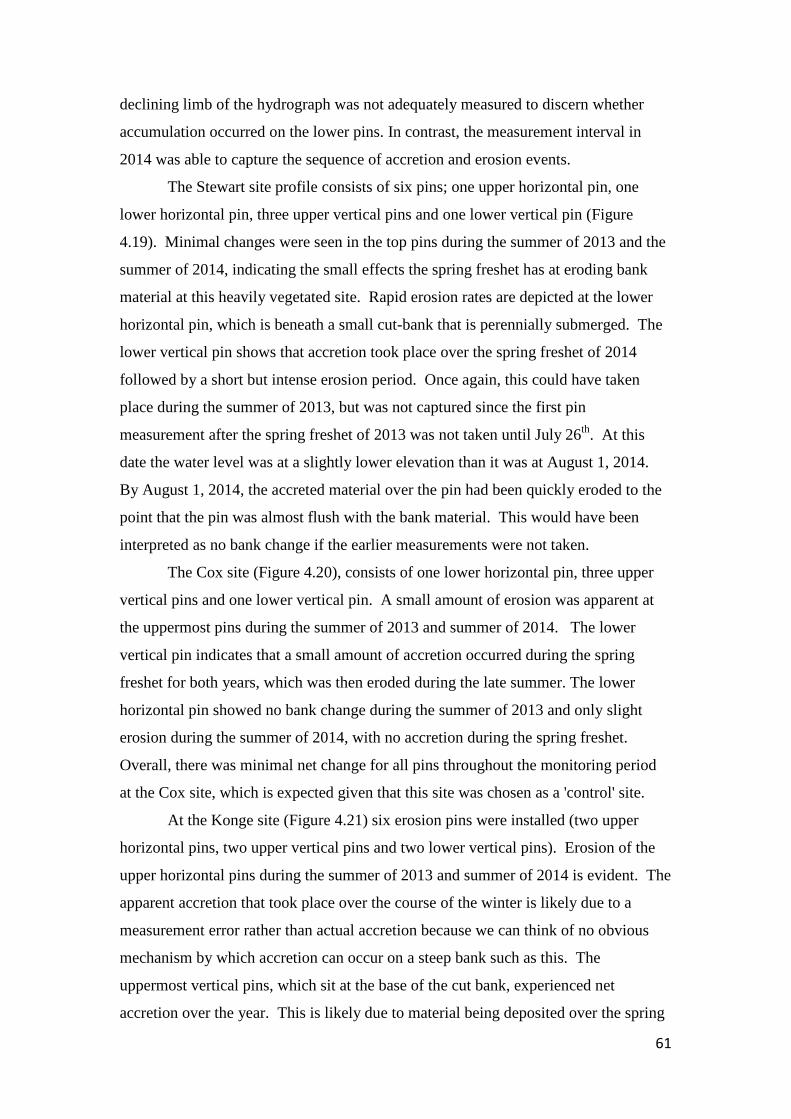
61

declining limb of the hydrograph was not adequately measured to discern whether

accumulation occurred on the lower pins. In contrast, the measurement interval in

2014 was able to capture the sequence of accretion and erosion events.

The Stewart site profile consists of six pins; one upper horizontal pin, one

lower horizontal pin, three upper vertical pins and one lower vertical pin (Figure

4.19). Minimal changes were seen in the top pins during the summer of 2013 and the

summer of 2014, indicating the small effects the spring freshet has at eroding bank

material at this heavily vegetated site. Rapid erosion rates are depicted at the lower

horizontal pin, which is beneath a small cut-bank that is perennially submerged. The

lower vertical pin shows that accretion took place over the spring freshet of 2014

followed by a short but intense erosion period. Once again, this could have taken

place during the summer of 2013, but was not captured since the first pin

measurement after the spring freshet of 2013 was not taken until July 26th. At this

date the water level was at a slightly lower elevation than it was at August 1, 2014.

By August 1, 2014, the accreted material over the pin had been quickly eroded to the

point that the pin was almost flush with the bank material. This would have been

interpreted as no bank change if the earlier measurements were not taken.

The Cox site (Figure 4.20), consists of one lower horizontal pin, three upper

vertical pins and one lower vertical pin. A small amount of erosion was apparent at

the uppermost pins during the summer of 2013 and summer of 2014. The lower

vertical pin indicates that a small amount of accretion occurred during the spring

freshet for both years, which was then eroded during the late summer. The lower

horizontal pin showed no bank change during the summer of 2013 and only slight

erosion during the summer of 2014, with no accretion during the spring freshet.

Overall, there was minimal net change for all pins throughout the monitoring period

at the Cox site, which is expected given that this site was chosen as a 'control' site.

At the Konge site (Figure 4.21) six erosion pins were installed (two upper

horizontal pins, two upper vertical pins and two lower vertical pins). Erosion of the

upper horizontal pins during the summer of 2013 and summer of 2014 is evident. The

apparent accretion that took place over the course of the winter is likely due to a

measurement error rather than actual accretion because we can think of no obvious

mechanism by which accretion can occur on a steep bank such as this. The

uppermost vertical pins, which sit at the base of the cut bank, experienced net

accretion over the year. This is likely due to material being deposited over the spring

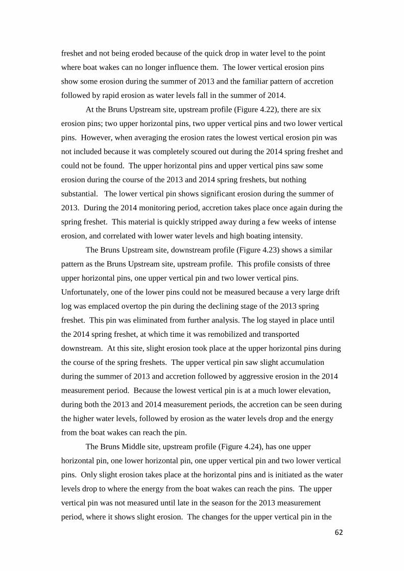
62

freshet and not being eroded because of the quick drop in water level to the point

where boat wakes can no longer influence them. The lower vertical erosion pins

show some erosion during the summer of 2013 and the familiar pattern of accretion

followed by rapid erosion as water levels fall in the summer of 2014.

At the Bruns Upstream site, upstream profile (Figure 4.22), there are six

erosion pins; two upper horizontal pins, two upper vertical pins and two lower vertical

pins. However, when averaging the erosion rates the lowest vertical erosion pin was

not included because it was completely scoured out during the 2014 spring freshet and

could not be found. The upper horizontal pins and upper vertical pins saw some

erosion during the course of the 2013 and 2014 spring freshets, but nothing

substantial. The lower vertical pin shows significant erosion during the summer of

2013. During the 2014 monitoring period, accretion takes place once again during the

spring freshet. This material is quickly stripped away during a few weeks of intense

erosion, and correlated with lower water levels and high boating intensity.

The Bruns Upstream site, downstream profile (Figure 4.23) shows a similar

pattern as the Bruns Upstream site, upstream profile. This profile consists of three

upper horizontal pins, one upper vertical pin and two lower vertical pins.

Unfortunately, one of the lower pins could not be measured because a very large drift

log was emplaced overtop the pin during the declining stage of the 2013 spring

freshet. This pin was eliminated from further analysis. The log stayed in place until

the 2014 spring freshet, at which time it was remobilized and transported

downstream. At this site, slight erosion took place at the upper horizontal pins during

the course of the spring freshets. The upper vertical pin saw slight accumulation

during the summer of 2013 and accretion followed by aggressive erosion in the 2014

measurement period. Because the lowest vertical pin is at a much lower elevation,

during both the 2013 and 2014 measurement periods, the accretion can be seen during

the higher water levels, followed by erosion as the water levels drop and the energy

from the boat wakes can reach the pin.

The Bruns Middle site, upstream profile (Figure 4.24), has one upper

horizontal pin, one lower horizontal pin, one upper vertical pin and two lower vertical

pins. Only slight erosion takes place at the horizontal pins and is initiated as the water

levels drop to where the energy from the boat wakes can reach the pins. The upper

vertical pin was not measured until late in the season for the 2013 measurement

period, where it shows slight erosion. The changes for the upper vertical pin in the

63

2014 measurement period are much more dramatic, showing substantial accretion

over the spring freshet. As water levels drop, boat wakes quickly erode the bank

material. The lower vertical pin shows the same trend, although on an even greater

scale. The pattern for this pin is also captured during the 2013 season as well as the

2014 measurement period.

The Bruns Middle site, downstream profile (Figure 4.25) has one upper

horizontal pin, one lower horizontal pin, one upper vertical pin and two lower vertical

pins. The upper horizontal pin shows a slumping event that took place between July

25 and August 1, 2014. This time range started with the water level at a similar

elevation to the pin, but then dropped quickly throughout the week. This slumping

event was likely caused by the saturated bank material no longer being supported by

the high water level. When the weight became too much, a large portion of the bank

broke off. At the lower horizontal pin, significant erosion took place over the 2013

spring freshet. However, throughout the winter, material was redeposited. During the

2014 measurement period, accretion followed by erosion occurred, although over the

entire measurement period there was no net bank change. The upper vertical pin

shows that in 2013, only slight accretion occurred. Over the winter, significant

erosion scoured the bank, but the spring freshet of 2014 deposited a healthy amount of

material, reburying the pin. As the summer wore on and water levels dropped, this

material was eroded out and net erosion occurred. Finally, the lower vertical pins

show the familiar pattern of accreted material when water levels are high, and erosion

of the bank as the water levels fall. Overall, the lower vertical pins show minimal net

change.

And lastly, the Bruns Downstream site (Figure 4.26), containing two upper

horizontal pins, two upper vertical pin, one middle vertical pin and one lower vertical

pin also had dramatic bank changes throughout the measurement period. At the upper

horizontal pins, slight erosion occurred during the 2013 spring freshet, followed by

accretion over the winter months. During the summer of 2014, a slumping event at

one of the pins was a source of major erosion. The upper vertical pins show minimal

changes over the summer of 2013, but once again, a pattern may have been missed

since measurements took place at a lower water elevation. In 2014, it is clear that

accretion took place over the spring freshet followed by a quick burst of erosion that

brought the bank back to the original elevation. The middle vertical pin shows in

both the 2013 and 2014 season that accretion occurs when water levels are high,

64

followed by erosion when water levels drop. This pattern is also seen in the lower

vertical pin, but the effects are delayed since it is at a lower elevation.

Figure 4.18 Cumulative bank change and rate of bank change at the DeRuiter Site. Note that the upper portions of the bank are differentiated from the lower portions of the bank and the pins measurements that have been averaged are in brackets

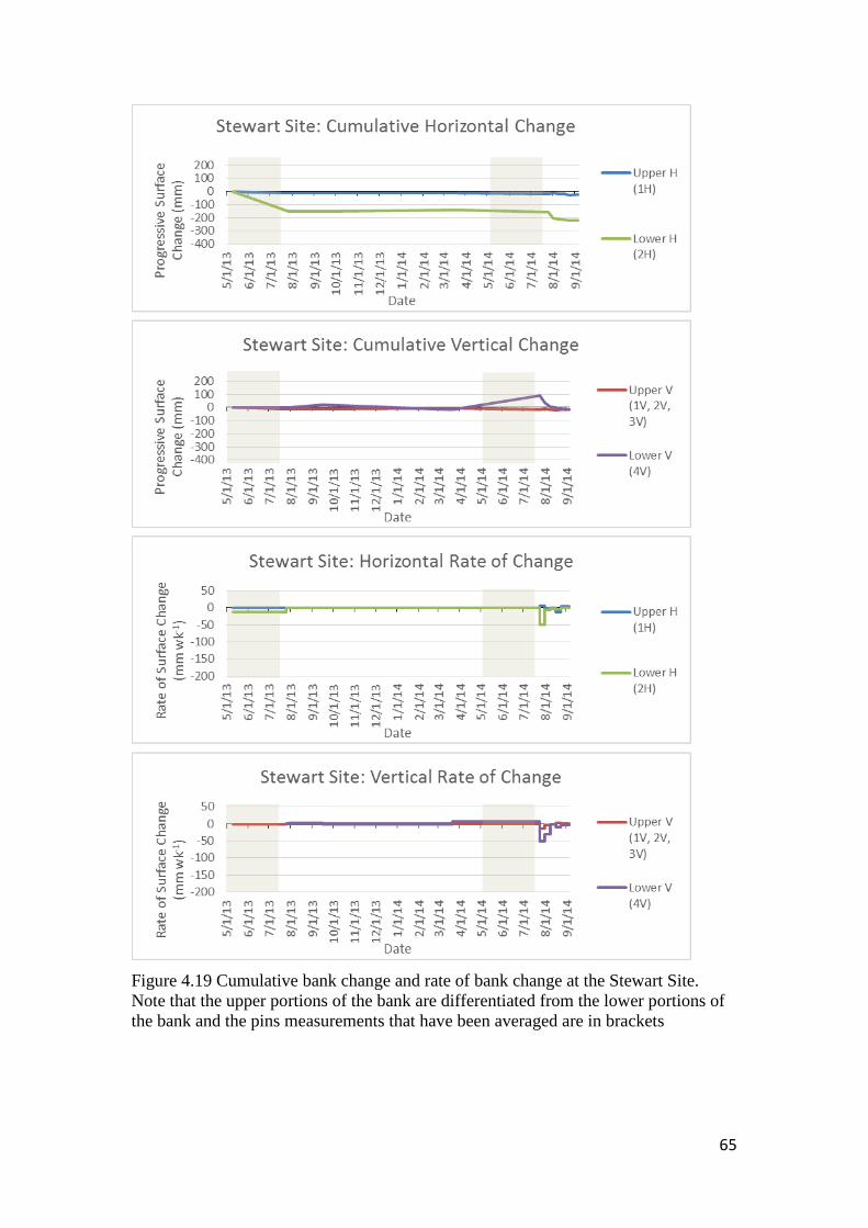
65

Figure 4.19 Cumulative bank change and rate of bank change at the Stewart Site. Note that the upper portions of the bank are differentiated from the lower portions of the bank and the pins measurements that have been averaged are in brackets

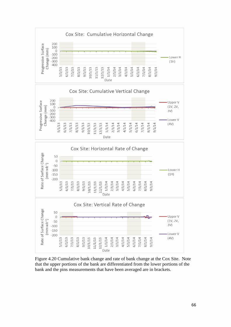
66

Figure 4.20 Cumulative bank change and rate of bank change at the Cox Site. Note that the upper portions of the bank are differentiated from the lower portions of the bank and the pins measurements that have been averaged are in brackets.

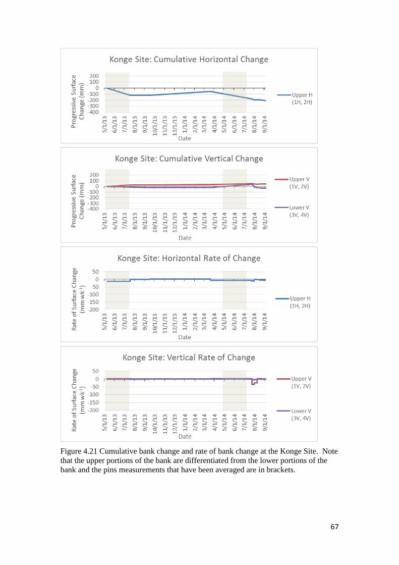
67

Figure 4.21 Cumulative bank change and rate of bank change at the Konge Site. Note that the upper portions of the bank are differentiated from the lower portions of the bank and the pins measurements that have been averaged are in brackets.

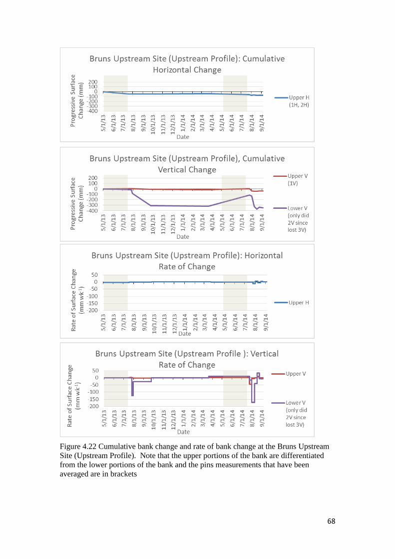
68

Figure 4.22 Cumulative bank change and rate of bank change at the Bruns Upstream Site (Upstream Profile). Note that the upper portions of the bank are differentiated from the lower portions of the bank and the pins measurements that have been averaged are in brackets

69

Figure 4.23 Cumulative bank change and rate of bank change at the Bruns Upstream Site (Downstream Profile). Note that the upper portions of the bank are differentiated from the lower portions of the bank and the pins measurements that have been averaged are in brackets

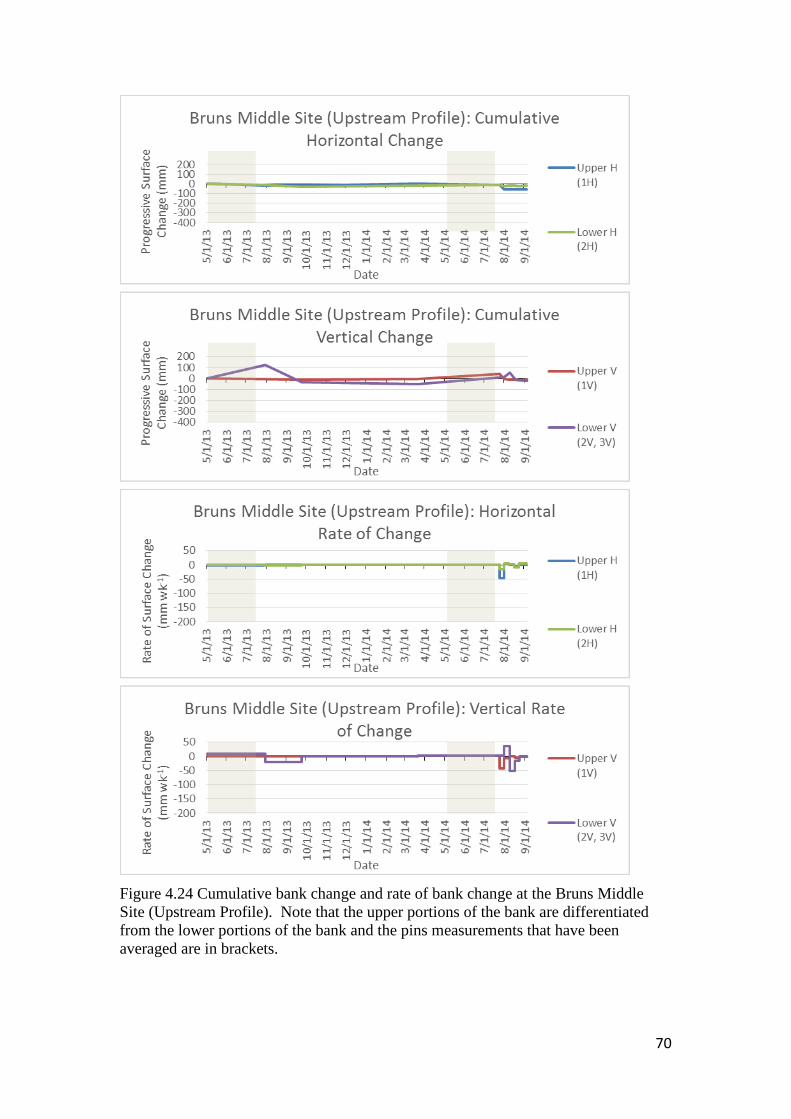
70

Figure 4.24 Cumulative bank change and rate of bank change at the Bruns Middle Site (Upstream Profile). Note that the upper portions of the bank are differentiated from the lower portions of the bank and the pins measurements that have been averaged are in brackets.

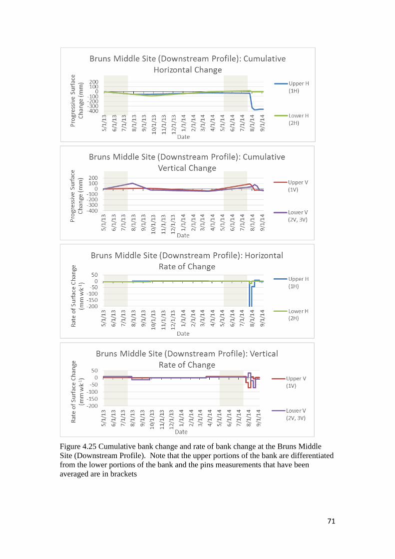
71

Figure 4.25 Cumulative bank change and rate of bank change at the Bruns Middle Site (Downstream Profile). Note that the upper portions of the bank are differentiated from the lower portions of the bank and the pins measurements that have been averaged are in brackets

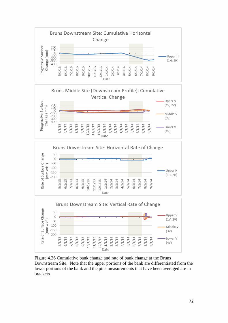
72

Figure 4.26 Cumulative bank change and rate of bank change at the Bruns Downstream Site. Note that the upper portions of the bank are differentiated from the lower portions of the bank and the pins measurements that have been averaged are in brackets

73

5. Discussion and Conclusion Laderoute and Bauer (2013) conducted an in-depth experiment that assessed

the impact of boat wakes on bank erosion along the Lower Shuswap River during the

summer of 2013. Their methodology included tracking the number of boats travelling

along the river at upstream and downstream locations using a camera, and monitoring

bank change using a network of erosion pins. Although bank erosion was observed in

that study, the data were inconclusive as regards to the overall impact of boating

traffic within the annual cycle of bank change because their methodology was not

developed for the purpose of quantifying the potential impact of the spring freshet on

bank erosion. Although the erosion pin network was installed prior to the spring

freshet of 2013, by the time the pins could be accessed safely to measure bank change

(late July), the boating season was already well under way. Consequently, any bank

change that was measured in late July could have been due to the spring freshet or to

boat wake activity (or potentially a combination of both). The project described in this

report was therefore designed to quantify the amount of shear stress exerted on the

banks during the spring freshet. At the same time, bank erosion and boat traffic

monitoring was conducted to extend the time series initiated by Laderoute and Bauer

(2013).

Boat traffic was monitored from May 23 to September 5, 2014. Overall,

speedboats were the most common vessels observed on the river, followed by PWCs

and then pontoon boats. The general trend shows boating traffic beginning to

increase around late June, coming to a peak at the beginning of August, and quickly

declining throughout the month of August. Despite ideal boating weather in August,

boating intensity dropped in accord with declining water levels in the river. The low

water levels pose a threat to watercraft and water skiers, which explains the decrease

in the number of speed boat passages. PWCs, in contrast, sit much higher in the water

and are able to operate in shallow reaches, which explains the increasing ratio of

PWCs to other watercraft near the end of the summer. By early September, the

boating season had effectively ceased. These trends resemble those of 2013, which

suggests that the traffic intensity patterns are approximately the same from year to

year.

The Bruns site, which receives a large number of boats from Mara Lake, had

significantly more watercraft passages than the De Ruiter site, which was located

74

much farther upstream. Boaters often travel from Mara Lake and up the Shuswap

River to explore or to use the calm waters for water skiing, but tend not venture as far

as Grindrod or Enderby. The vessel passages at the De Ruiter site are likely

associated with local landowners who maintain riverside docks or with boaters who

launched at the Enderby boat launch.

Despite an overall increase in total watercraft passages during the 2014

monitoring period relative to 2013 (increases of 839 and 92 vessel passages at the

Bruns and DeRuiter site respectively), there was slightly more bank erosion during

the 2013 boating season. The implication is that there is not a straightforward, linear

relationship between boat traffic intensity and river bank erosion, and that other

factors must be at play. Previous studies (e.g., Houser, 2010; Osborne et al., 2007;

Bauer et al., 2002; Parnell and Kofed-Hansen, 2001) indicate that bank erosion

depends on boat length, boat speed, hull displacement, and sailing distance from the

bank, which are difficult parameters to quantify for every boat passage. In addition,

there may be additional natural processes that cause bank erosion, such as slumping

and mass wasting. Bank structure, soil moisture content, material strength,

vegetation cover, and the river flow patterns must also be accounted for. For

example, more erosion may have occurred in the 2013 because the spring freshet

drawdown period was more rapid than in 2014. The saturated bank material would

have been left unsupported by the quick decrease in water stage, resulting in mass

wasting events. Estimating riverbank erosion can focus on many different aspects but

this experiment focused on only two primary factors: boating intensity and shear

stress. It is important to realize that there are numerous other factors that may impact

the change of bank geomorphology along the Lower Shuswap River.

Frequently, flume studies are preformed to minimize the variables affecting

the fluid flow properties (e.g., Hopkinson and Wynn-Thompson, 2012; Kean et al.,

2009; Czernuszenko and Holley, 2007; Thompson et al., 2004; Song and Chiew,

2001; Tominaga and Nezu, 1991). The purpose of this is to collect data that is easy to

analyse. However, the results from flume experiments may not apply directly to

natural channels. Natural channels lack the simple, smooth geometries commonly

used in flumes, and almost never have the uniform flow used in lab experiments

(Papanicolaou et al. 2007). Frequently, the theories on fluid flow characteristics

produced in lab experiments do not align with what is seen in the natural

environment, as in the case with our collected data. Typically, shear stress is greatest

75

at the bed and decreases linearly with distance from the bottom, but the Reynolds

method in this analysis produced a shear stress profile showing the opposite results

(shear stress increasing with distance from the bed). Our interpretation of this trend is

that the particular location in which measurements were taken was a relatively slack-

water environment with minimal downstream flow velocities. As a consequence, the

velocity gradients were rather minimal away from the bank and there was relatively

little shear stress to be expended. The increasing Reynolds stress values away from

the bank are due to the greater correlation between the horizontal and vertical flow

components in the main body of the flow (i.e., farther away from the bank) whereas

closer to the bank the flow components are randomly distributed with little

correlation. These observations, which are contrary to established theoretical ideas

about how boundary layers are structured, emphasizes the importance of collecting

data in situ for assessing river bank erosion processes. Even though the measured

shear stress profiles do not line up with theoretical predictions, the data are sound,

reliable and accurately reflect the flow characteristics at the measuring site.

There is some disagreement in the scientific community about how best to

process velocity data in order to make boundary shear stress estimates. Some

researchers say that the Law of the Wall method produces the best results (e.g.

Hopkinson and Wynn-Thompson, 2012; Andersen et al., 2007) and others claim that

the Reynolds Stress method should be used when working in the natural environment

(e.g. Sulaiman et al., 2013). In this study, both techniques were used and we conclude

that the Law of the Wall method produced more reliable results as regards shear stress

trends on the banks.

There is good reason to conclude that the impact of high flows during the

spring freshet are not effective in eroding the banks along the Lower Shuswap River.

The ADV measurements on June 2, 2014 at the Bruns Middle site during the height of

the freshet indicate that the shear stresses are remarkably small along the river bank.

In fact, both the Law of the Wall method and the Reynolds Stress method yield shear

stress values that are far too small to initiate sediment erosion at these locations. The

measurements on July 18, during the declining limb of the spring freshet, produced

similar results. As a consequence, it is reasonable to conclude that relatively little

bank change takes place during the high flow portions of the spring freshet,

presuming there are no bank slumping events during the height of the freshet. The

76

same may not be true for other sites along the Lower Shuswap River, particularly

those on the outer banks of extreme meander bends.

Figure 5.1 shows the trends in river stage and boating traffic at the Bruns site

from the height of the spring freshet to the conclusion of the boating season during

2014. It is readily apparent that there is considerable overlap between the declining

limb of the spring freshet and the ramp-up period of the boating season (June through

mid-July). Until about mid-July, the impact of boat-wake waves is restricted to the

upper portions of the bank exclusively by virtue of the high water levels (above 3 m

relative stage). However, from mid-July to mid-August, which corresponds to the

peak of the boating season, the water level drops rapidly from the mid-upper bank

position to the lower bank position (about 2 m relative stage), and this implies that a

one metre vertical swath of bank can be impacted by boat waves in intensely

repetitive fashion over about three weeks. It is important to note that measurement of

the erosion pins was not possible until the river stage dropped to a safe level (below

2.8 m relative stage), and therefore the first measurements of 2014 were not possible

until July 25, at which time several of the lowermost pins on the profiles were still

inaccessible. Subsequent pin measurements were taken on August 1, 9, 17, 24, and

September 5 (as marked on Figure 5.1), which coincides with low stage and declining

boat traffic intensity. The relative timing of these trends reveals that there is a period

from mid-June through mid-July for which there are no pin erosion measurements but

when the impact of the spring freshet and enhanced boating traffic work in concert.

This appears to be a critical period as regards bank erosion during the annual cycle of

bank change for which we still lack detailed data.

Figures 5.2 and 5.3 are conceptualized renditions of the processes taking place

along the Bruns Middle Site (Upstream Profile) during and after the freshet, which

also reflects what was observed at other profiles. Based on the ADV measurements

and shear stress calculations, it was assumed that no erosion takes place during the

high flow period in late June and early July. Boat wakes are relatively unimportant

during high flows because there are very few boats (see Tables 4.1 and 4.2) and

because the impact of any boat-wake waves is restricted to the uppermost portions of

the bank. The influence of these waves does not extend to the bottom of the profile

because they are of short wavelength and the orbital velocity field decreases rapidly

with depth. Therefore, it is assumed that the bank morphology remained the same

during the high discharge period.

77

Figure 5.1 River stage at the Enderby gauging station, recorded by the Environment Canada, Water Office (2014), compared to weekly averaged boat counts at the Bruns Site during the summer of 2014

As water levels begin to fall in mid-June to mid-July, boating intensity begins

to become more significant (Figure 5.1). During this period, the moderate intensity of

boat traffic yields bank erosion along the upper and middle portions of the river bank

(Figure 5.2). As before, the lower portions of the bank and the river bed remain

relatively undisturbed because the waves from boats aren't of sufficient magnitude to

influence the bottom. However, the material that is eroded from the upper and middle

parts of the profile is deposited on the lower apron (horizontal portions of the bank

and bed). Even though the discharge levels are still high, the velocity of the flow near

the banks is too small to entrain sediment. As a consequence, a thin layer of accretion

(approximately 0.02 – 0.08 m in thickness) evolves on the apron during July, whereas

localized erosion takes place in the non-vegetated portions of the upper and middle

bank (usually in association with previous slumping scarps.

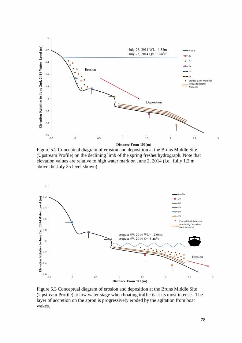
78

Figure 5.2 Conceptual diagram of erosion and deposition at the Bruns Middle Site (Upstream Profile) on the declining limb of the spring freshet hydrograph. Note that elevation values are relative to high water mark on June 2, 2014 (i.e., fully 1.2 m above the July 25 level shown)

Figure 5.3 Conceptual diagram of erosion and deposition at the Bruns Middle Site (Upstream Profile) at low water stage when boating traffic is at its most intense. The layer of accretion on the apron is progressively eroded by the agitation from boat wakes.

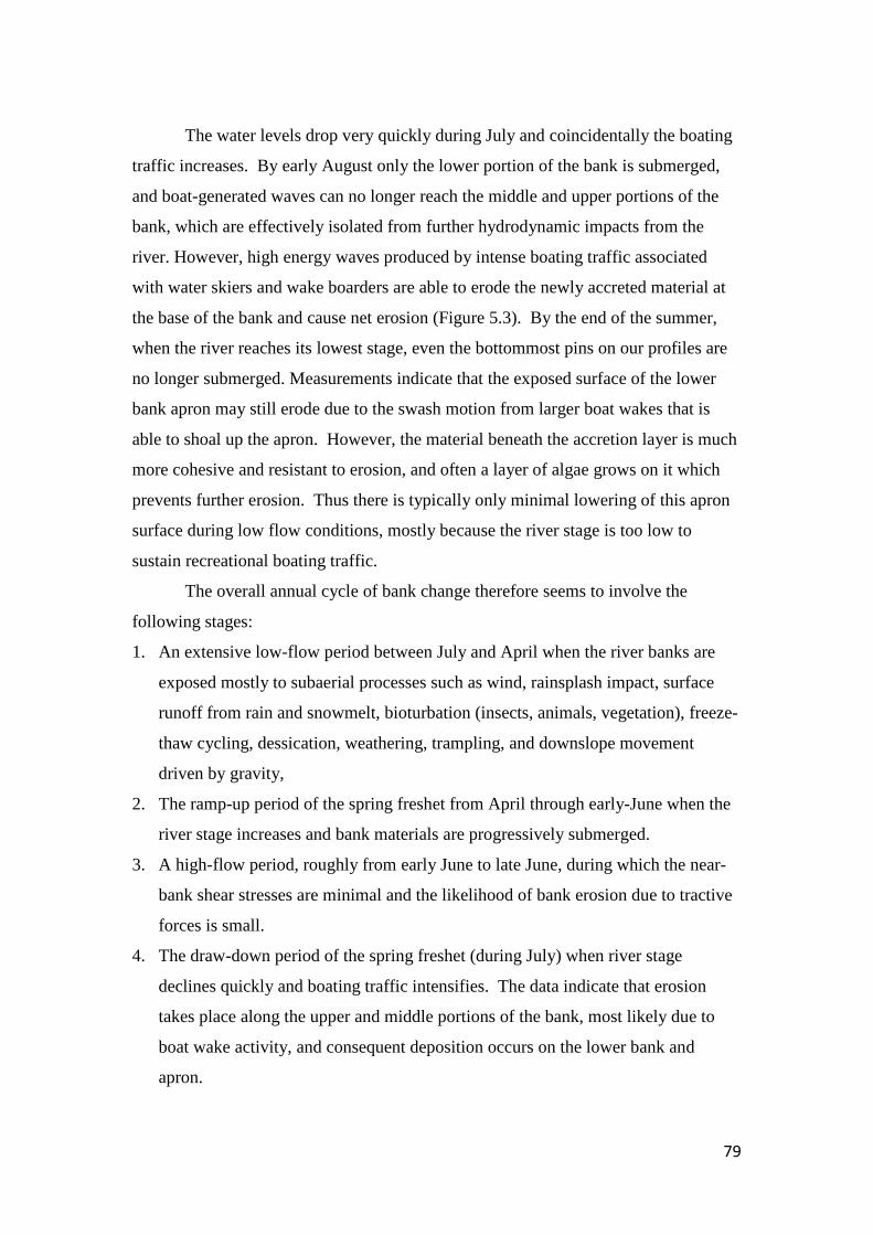
79

The water levels drop very quickly during July and coincidentally the boating

traffic increases. By early August only the lower portion of the bank is submerged,

and boat-generated waves can no longer reach the middle and upper portions of the

bank, which are effectively isolated from further hydrodynamic impacts from the

river. However, high energy waves produced by intense boating traffic associated

with water skiers and wake boarders are able to erode the newly accreted material at

the base of the bank and cause net erosion (Figure 5.3). By the end of the summer,

when the river reaches its lowest stage, even the bottommost pins on our profiles are

no longer submerged. Measurements indicate that the exposed surface of the lower

bank apron may still erode due to the swash motion from larger boat wakes that is

able to shoal up the apron. However, the material beneath the accretion layer is much

more cohesive and resistant to erosion, and often a layer of algae grows on it which

prevents further erosion. Thus there is typically only minimal lowering of this apron

surface during low flow conditions, mostly because the river stage is too low to

sustain recreational boating traffic.

The overall annual cycle of bank change therefore seems to involve the

following stages:

1. An extensive low-flow period between July and April when the river banks are

exposed mostly to subaerial processes such as wind, rainsplash impact, surface

runoff from rain and snowmelt, bioturbation (insects, animals, vegetation), freeze-

thaw cycling, dessication, weathering, trampling, and downslope movement

driven by gravity,

2. The ramp-up period of the spring freshet from April through early-June when the

river stage increases and bank materials are progressively submerged.

3. A high-flow period, roughly from early June to late June, during which the near-

bank shear stresses are minimal and the likelihood of bank erosion due to tractive

forces is small.

4. The draw-down period of the spring freshet (during July) when river stage

declines quickly and boating traffic intensifies. The data indicate that erosion

takes place along the upper and middle portions of the bank, most likely due to

boat wake activity, and consequent deposition occurs on the lower bank and

apron.

80

5. A low-flow period during most of August when water stage is at the lower bank

and when boat traffic is at its most intense. During this state, the layer of

deposition on the apron is progressively eroded and the sediment is moved

downstream and into the deeper sections of the main channel.

The cumulative effect of this annual cycle of bank change is that there is net

erosion of the bank, mostly through horizontal retreat of the upper and middle

portions of the bank. There may also be progressive reduction of the apron in years

when the boating traffic is particularly intense during August. And there is always the

potential for slumping events to occur, typically during the draw-down period when

the bank materials are fully saturated. Bank slumping is particularly pronounced in

locations where there has been erosion at the base of the bank by wave action in the

previous boating seasons, which leads to greater instability of the bank.

The data collected during this study make it quite evident that the high

discharge flows during the spring freshet are not capable of significantly altering bank

structure at sites that are comparable to the Bruns site. The implication is that boat-

generated waves may be of relatively greater importance in forcing bank change

throughout the annual cycle than had previously been anticipated. Our data regarding

the timing and location of erosion and deposition relative to the intensification of the

boating season provide valuable information in regards to management strategies

directed at mitigating potential damage to the riparian zones along the Lower

Shuswap River.

81

6. Bibliography

Andersen, T.J., Fredsoe, J., and Pejrup, M. (2007). In situ estimation of erosion and deposition thresholds by Acoustic Doppler Velocimeter (ADV). Estuarine, Coastal and Shelf Science, 75(3), 327-336. Doi: 10.1016/j.ecss.2007.04.039. Retrieved from http://www.sciencedirect.com/science/article/pii/S0272771407001990

Bauer, B., Lorang, M., and Sherman, D. (2002). Estimating boat-wake-induced levee

erosion using sediment suspension measurements. Journal of Waterway, Port, Coastal, and Ocean Engineering, 128(4), 152-162. Doi: 10.1061/(ASCE)0733-950X(2002)128:4(152)

Bauer, B., Sherman, D., and Wolcott, J. (1992). Sources of Uncertainty in Shear

Stress and Roughness Length Estimates Derived from Velocity Profiles. Professional Geographer, 44(4), 453-464.

Buffin- Bélanger, T., and Roy, A.G. (2005). 1 min in the life of a river: selecting the

optimal record length for the measurement of turbulence in fluvial boundary layers. Geomorphology, 66(1-2), 77-94. Doi: 10.1016/j.geomorph.2004.09.032 Retrieved from http://www.sciencedirect.com/science/article/pii/S0169555X04002909#

Clark, L.A., and Wynn, T.M. (2007). Methods for determining streambank critical

shear stress and soil erodibility: implications for erosion rate predictions. Transactions of the ASABE, 50(1), 95-106. Doi: 10.13031/2013.22415. Retrieved from http://www.tmdl.bse.vt.edu/uploads/File/Pub%20db%20files%20stream%20rest/Clark_Wynn_2007TransASABE.pdf

Constantine, C., Dunne, T., and Hanson, G. (2009). Examining the Physical Meaning

of the Bank Erosion Coefficient Used in Meander Migration Modeling. Geomorphology, 106(3-4), 243-252. Doi: 10.1016/j.geomorph.2008.11.002

Curran, J., and McTeague, M. (2011). Geomorphology and Bank Erosion of the

Matanuska River, Southcentral Alaska. U.S. Geological Survey Investigations Report 2011-5214, 52p. Retrieved from http://pubs.usgs.gov/sir/2011/5214/pdf/sir20115214.pdf

Czernuszenko, W. and Holley, E. (2007). Open-Channel Turbulence Measurements

with a Three-Component Acoustic Doppler Velocimeter. Publications of the Institute of Geophysics, Polish Academy of Sciences, E-7 (401), 31p. Retrieved from http://agp2.igf.edu.pl/agp/files/E-7/Czernuszenko_Holley.pdf

Debnath, K., Nikora, V., and Elliott, A. (2007). Stream Bank Erosion: In Situ Flume

Tests. Journal of Irrigation and Drainage Engineering, 33(3), 257-264.

82

Retrieved from http://ascelibrary.org/doi/full/10.1061/%28ASCE%290733-9437%282007%29133%3A3%28256%29

Duan, J. (2005). Analytical Approach to Calculate Rate of Bank Erosion. Journal of

Hydraulic Engineering, 131(11), 980-990. Retrieved from http://ascelibrary.org/doi/abs/10.1061/%28ASCE%290733-9429%282005%29131%3A11%28980%29

Einstein, A. (1926). Ursache der Meanderbildung der Flusslaufe und des sogenannten

Baerschen Gesetzes. Naturwissenschaften, 14 (11), 223-224 Doi: 10.1007/BF01510300

Environment Canada, Wateroffice (2014). Real-time data: Shuswap River near

Enderby (08LC002). Retrieved from http://www.wateroffice.ec.gc.ca/graph/graph_e.html?stn=08LC002

EPA United States Environmental Protection Agency. (2012). Channel Processes:

Streambank Erosion. Retrieved from http://water.epa.gov/scitech/datait/tools/warsss/streamero.cfm

Fredsoe, J. (1990): Hydrodynamik, Den private Ingeniørfond, Danmarks tekniske

Højskole, Stougaard Jensen, København. Figure retrieved from http://daad.wb.tu-harburg.de/tutorial/flood-probability-assessment/hydrodynamics-of-floods/2d-hydrodynamic-models/theory/fundamentals-of-mathematical-river-flow-modelling-2d-flow-calculation/turbulent-flows/reynolds-average-navier-stokes-equation/

Gamesby, R. (2013). Meanders, oxbow lakes and flood plains. Geography

Department of Lord Wandsworth College. Retrieved from http://www.coolgeography.co.uk/GCSE/Year%2010/PhysicalWorld/Middle%20valley/landforms_of_the_middle_reaches.htm

Gardiner, T. (1983). Some Factors Promoting Channel Bank Erosion, River Lagan,

County Down. Journal of Earth Sciences, 5(2), 231-239. Retrieved from http://www.jstor.org/stable/30002167?seq=2

Hopkinson, L., and Wynn-Thompson, T. (2012). Streambank shear stress estimates

using turbulent kinetic energy. Journal of Hydraulic Research, 50(3), 320-323. Doi: 0.1080/00221686.2012.684771. Retrieved from http://www.tandfonline.com/doi/pdf/10.1080/00221686.2012.684771

Houser, C. (2010). Relative Importance of Vessel-Generated and Wind Waves to Salt

Marsh Erosion in a Restricted Fetch Environment. Journal of Coastal Research, 26(2), 230-240. Doi: 10.2112/08-1084.1

Ikeda, S., Parker, G., Sawai, K. (1981). Bend theory of river meanders: part I, Linear

development. Journal of Fluid Mechanics, 112, 363–377. Retrieved from

83

http://journals.cambridge.org/action/displayFulltext?type=1&fid=375705&jid=FLM&volumeId=112&issueId=-1&aid=375704

Kean, J.W. and Smith J.D., (2006a). Form drag in rivers due to small-scale natural

topographic features: 1. Regular sequences. Journal of Geophysical Research, 111, F04009. Doi: 10.1029/2006JF000467

Kean, J.W., Smith, J.D. (2006b). Form drag in rivers due to small-scale natural

topographic features: 2. Irregular sequences. Journal of Geophysical Research, 111, F04010. Doi: 10.1029/2006JF000490

Kean, J., Kuhnle, R., Smith, D., Alonso, C., and Langerdoen, E. (2009). Test of a

Method to Calculate Near-Bank Velocity and Boundary Shear Stress. Journal of Hydraulic Engineering, 135(7), 588-601. Retrieved from http://ascelibrary.org/doi/abs/10.1061/%28ASCE%29HY.1943-7900.0000049

Kitanidis, P., and Kennedy, J. (1984). Secondary Current and River-Meander

Formation. Journal of Fluid Mechanics, 144, 217-229. Doi: 10.1017/S0022112084001580

Knighton, D. (1998). Fluvial Forms and Processes: A New Perspective. London:

Hodder Education. ISBN: 978 0 340 66313 4 Kramer, Bernhard. (2003). Shuswap Lake Spring Flood Watch Program. Retrieved

from http://www.shuswaplakewatch.com/research/river2.html Lauderoute, L., and Bauer, B. (2013). River Bank Erosion and Boat Wakes Along the

Lower Shuswap River, British Columbia. Final Project Report submitted to Regional District of North Okanagan Fisheries and Oceans Canada. Retrieved from http://www.rdno.ca/docs/River_Bank_Erosion_Lower_Shu_River_Final_Project_Report.pdf

Laderoute, L. (2014). River Bank Erosion and Boat Wakes Along the Lower Shuswap

River, British Columbia (Bachelor’s Thesis). Honours thesis paper submitted to the University of British Columbia (Okanagan).

McCuen, R. (2004). Hydrologic Analysis and Design: Third Edition. New Jersey:

Pearson Education. ISBN: 0 13 142424 6 Motta, D., Langendoen, E.J., Abad, J.D., and García, M.H. (2014). Modification of

Meander Migration by Bank Failures. Journal of Geophysical Research: Earth Science, 119(5), 1026-1042. Doi: 10.1002/2013JF002952

Nelitz, M., Alexander, C.A.D., Wieckowski, K. (2007). Helping Pacific Salmon

Survive the Impace of Climate Change on Freshwater Habitats: Case Studies. Report Prepared for Pacific Fisheries Resource Conservation Council by ESSA Technologies Ltd. Retrieved from http://www.fish.bc.ca/files/PFRCC-ClimateChange-Adaptation-CaseStudies_Complete.pdf

84

Osborne, P., Hericks, D., and Côtè, J. (2007, September). Full-Scale Measurements of

High Speed Passenger Ferry Performance and Wake Signature. Paper presented at Oceans 2007, Vancouver, BC. Doi: 10.1109/OCEANS.2007.4449211

Papanicolaou, A., Maxwell A., Hilldale, R., Filipy J., and Peterschmidt, L. (2001).

Erosion of Cohesive Streambed and Banks. Project Completion Report Submitted to the State of Washington Water Research Center and the U.S. Geological Survey. Retrieved from http://www.academia.edu/3022884/Erosion_of_cohesive_streambeds_and_banks

Papanicolaou, A., Elhakeem, M., and Hilldale, R. (2007), Secondary current effects

on cohesive river bank erosion. Water Resources Research, 43, W12418. Doi: 10.1029/2006WR005763.

Parnell, K., and Kofed-Hansen, H. (2001). Wakes from Large High-Speed Ferries in

Confined Coastal Waters: Management Approaches with Examples from New Zealand and Denmark. Coastal Management, 29(3). Doi: 10.1080/08920750152102044

Pizzuto, J.E., and Meckelnburg, T.S. (1989). Evaluation of a Linear Bank Erosion

Equation. Water Resources Research, 25(5), 1005-1013. Posner, A., and Duan, J. (2012). Simulating River Meandering Processes Using

Stochastic Bank Erosion Coefficient. Geomorphology, 163-164. Pages 26-36. Retrieved from http://www.sciencedirect.com/science/article/pii/S0169555X11003059

River bank failure. (2014, September 7). In Wikipedia, The Free Encyclopedia.

Retrieved September 24, 2014, from http://en.wikipedia.org/w/index.php?title=River_bank_failure&oldid=624510195

Shields, A. (1936). Anwendung der Aenlichkitsmechanik und der Turbulenzforshung

auf die Geschiebebewegung. Berlin: Mitteilungen der Prevssischen Versuchsanstalt fur Wasserbau und Schiffbau.

Shuswap Nation Tribal Council. (2014). Splatsin First Nation. Retrieved from

http://shuswapnation.org/bands/splatsin-enderby/ Shuswap River Watershed Sustainability Plan (2014). Regional District of the North

Okanagan. Retrieved from http://www.rdno.ca/docs/140408_SRWSP.pdf Simon, A., Pollen-Bankhead, N., Mahacek, V., and Langendoen, E. (2009).

Quantifying Reductions of Mass-Failure Frequency and Sediment Loadings from Streambanks Using Toe Protection and Other Means: Lake Tahoe, United States. Journal of the American Water Resources Association, 45(1), 170-186. Doi: 10.1111/j.1752-1688.2008.00268.

85

Song, T., and Chiew, Y.M. (2001). Turbulence Measurement in Nonuniform Open-

Channel Flow Using Acoustic Doppler Velocimeter (ADV). Journal of Engineering Mechanics, 127(3), 219-232.

Sulaiman, M.S., Sinnakaudan, S.K., and Shukor, M.R. (2013). Near Bed Turbulence

Measurement with Acoustic Doppler Velocimeter (ADV). KSCE Journal of Civil Engineering, 17(6), 1515-1528. Doi: 10.1007/s12205-013-0084-8

Thompson, A.m., Wilson, B.N., and Hansen, B.J. (2004). Shear stress partitioning for

idealized vegetated surfaces. Transactions of the ASAE, 47(3), 701-709. Doi: 10.13031/2013.16102.

TMDL (2006). Incorporating Channel Degradation and Restoration into Watershed

Models. Retrieved from http://www.tmdl.bse.vt.edu/stream_restoration/C115/ Tominaga, A. and Nezu, I. (1991). Turbulent Structure in Compound Open-Channel

Flows. Journal of Hydraulic Engineering, 117(1), 21-41. Retrieved from http://ascelibrary.org/doi/abs/10.1061/%28ASCE%290733-9429%281991%29117%3A1%2821%29

Trenhaile, A. (2010). Geomorphology: A Canadian Perspective (4th ed.). Don Mills,

Ontario: Oxford University Press. Voulgaris, G., and Trowbridge, J.H. (1997). Evaluation of the Acoustic Doppler

Velocimeter (ADV) for Turbulence Measurements. Journal of Atmospheric and Ocean Technology, 15, 272-289. Retrieved from http://journals.ametsoc.org/doi/pdf/10.1175/1520-0426(1998)015%3C0272%3AEOTADV%3E2.0.CO%3B2

Water Canada: The Complete Water Magazine. (2013, November 11). Alberta

Invests $116 Million in Flood Erosion Control. Retrieved from http://watercanada.net/2013/alberta-invests-116-million-in-flood-erosion-control/

Wojda, M. (2008). Bank erosion in the petitcodiac river estuary (Master’s thesis).

Retrieved from http://search.proquest.com.ezproxy.library.ubc.ca/docview/1365224039?accountid=14656. (1365224039).