sediment yield and bank erosion assessment of pra river ... yield... · this thesis entitled...

SEDIMENT YIELD AND BANK EROSION ASSESSMENT

OF PRA RIVER BASIN

BY

John Manyimadin Kusimi

(10096985)

This thesis is submitted to the University of Ghana, Legon in

partial fulfilment of the requirement for the award of PhD

Geography & Resource Development degree.

June, 2014

University of Ghana http://ugspace.ug.edu.gh

i

Declaration

This thesis entitled “Sediment yield and bank erosion assessment of Pra River Basin” is

entirely an original study that I conducted. With the exception of relevant literature and ideas of

specific sources which have been duly referenced, the work has not been presented anywhere in

part or whole for any award of a degree.

........................................................

John Manyimadin Kusimi

(Student)

(10096985)

Date...........................................

............................................................

Dr. Emmanuel Morgan Attua

Dept of Geography & Resource Dev’t

University of Ghana, Legon

(Principal supervisor)

Date...........................................

........................................................

Prof Bruce Banoeng-Yakubo

Department of Earth Science

University of Ghana, Legon

(Supervisor)

Date...........................................

...............................................................

Dr. Barnabas Amisigo

Water Research Institute

CSIR, Accra

(Supervisor)

Date...........................................


ii

DEDICATION

This work is dedicated to my family for their immense support, prayers and contribution.


iii

Acknowledgement

I am grateful to God for bringing me this far in life and academia; to my supervisors: Dr.

Emmanuel Morgan Attua, Dr. Barnabas Amisigo and Prof Bruce Banoeng-Yakubo for their

support, suggestions, patience and making time off their busy schedules to supervise my work.

The University of Ghana partially funded this thesis by awarding me a Faculty Development

Grant which was very helpful in undertaking the field work and meeting the costs of field data

analysis.

I will like to express my gratitude to my brother Jonathan Kusimi, wife Mrs. Bertha Kusimi

and Mr. Gabriel Appiah of Water Research Institute, CSIR – Accra for assisting me in my field

data collection.

I will wish to thank Water Research Institute, CSIR - Accra and Ecological Laboratory

(ECOLAB) of the Dept of Geography & Resource Development, University of Ghana for

providing field equipment and laboratory space to collect and analyze my field samples. The

support of Mr. Prince Owusu of ECOLAB during my field data analyses is also acknowledged.

Lastly, I wish to thank Mr. Gerald B. Yiran of the Dept of Geography & Resource

Development, University of Ghana for always responding to my call anytime I was in need of

assistance with respect to data processing and analysis on the modelling aspect of the thesis.


iv

List of Tables

Table Page

Table 2.1: Examples of models for the derivation of R values................................... 34

Table 3.1: Discharge Rating Curves............................................................................ 42

Table 3.2: Annual suspended sediment load and specific suspended sediment yield

for the monitored stations in the Pra River Basin................................................ 56

Table 3.3: Parameters for suspended sediment rating curves....................................... 57

Table 4.1: Mean 210

Pb Concentration levels for stream sediment and potential

source materials in Birim Basin........................................................................... 64

Table 4.2: Mean 210


source materials in Pra Basin............................................................................... 64

Table 4.3: Mean 210


source materials in Oda Basin............................................................................. 64

Table 4.4: Mean 210


source materials in Offin Basin............................................................................ 64

Table 4.5: Contribution of bank material and surface soil sources to suspended

sediment load in the various sub-catchments...................................................... 64

Table 5.1: Annual bank erosion or deposition rates at Anyinam................................. 75

Table 5.2: Annual bank erosion or deposition rates at Amuanda Praso....................... 75

Table 5.3: Annual bank erosion or deposition rates at Akim Oda.............................. 76

Table 5.4: Annual bank erosion or deposition rates at Brenase.................................. 76

Table 5.5: Annual bank erosion or deposition rates at Ejisu....................................... 76

Table5.6: Annual bank erosion or deposition rates at Adiembra................................ 77


v

Table 6.1A: K Factor Values of the Soil types............................................................. 86

Table 6.1B: Soil erodibility classification.................................................................... 86

Table 6.2: Land Cover Types and Cover Management (C) factor values.................... 88

Table 6.3: Attributes of Landsat ETM+ 2008............................................................. 88

Table 6.4: Land cover co-efficient values................................................................... 90

Table 6.5: Statistics of the different sediment yield model variables......................... 100

Table 6.6: Estimates of sensitivity analysis of sediment yield for 12 mm event......... 101

Table 6.7: Estimates of sensitivity analysis of sediment yield for 12.5 mm event....... 101

List of Figures

Figure Page

Fig.1.1: Map of the Pra River Basin........................................................................... 14

Fig.3.1: Sediment Yield Sampling Stations................................................................ 40

Fig.3.2: Daily mean concentration of samples at Anwiankwanta.............................. 44

Fig.3.3: Daily mean concentration of samples at Brenase........................................... 44

Fig.3.4: Daily mean concentration of samples at Akim Oda....................................... 45

Fig.3.5: Daily mean concentration of samples at Adiembra....................................... 45

Fig.3.6: Daily mean concentration of samples at Twifo Praso.................................... 46

Fig.3.7: Daily mean concentration of samples at Assin Praso.................................... 46

Fig.3.8: Daily mean concentration of samples at Sekyere Heman.............................. 47

Fig.3.9: Mean monthly sediment load at Akim Oda................................................... 50

Fig.3.10: Mean monthly sediment load at Brenase..................................................... 50

Fig.3.11: Mean monthly sediment load at Anwiankwanta......................................... 51


vi

Fig.3.12: Mean monthly sediment load at Adiembra.................................................. 51

Fig.3.13: Mean monthly sediment load at Twifo Praso.............................................. 52

Fig.3.14: Mean monthly sediment load at Assin Praso............................................... 52

Fig.3.15: Mean monthly sediment load at Sekyere Heman......................................... 53

Fig.3.16: Annual sediment yield. ............................................................................... 56

Fig.5.1: Particle size distribution curves of bank sediments....................................... 80

Fig.5.2: Eroded bank sediments.................................................................................. 82

Fig.6.1: Schematic chart of GIS applications to soil erosion mapping and the

derivation of Sediment Delivery Ratio, SDR.............................................................. 84

Fig.6.2: Effective total rainfall erosivity (Re) factor map of 2008 for 12 mm............ 92

Fig.6.3: Effective total rainfall erosivity (Re) factor map of 2008 for 12.5 mm......... 92

Fig.6.4: The soil erodibility (K) map of the basin........................................................ 92

Fig.6.5: The length and slope (LS) map of the basin................................................... 92

Fig.6.6: Cover management factor (C) map derived from satellite image

classification....................................................................................................... 93

Fig.6.7: Soil erosion potential map of the basin.......................................................... 93

Fig.6.8: Gross soil erosion map of 12 mm erosive event............................................ 95

Fig.6.9: Gross soil erosion map of 12.5 mm erosive event......................................... 95

Fig.6.10: Sediment delivery ratio map of the basin................................................... 95

Fig.6.11: Sediment yield map of 12 mm erosive event.............................................. 95

Fig.6.12: Sediment yield map of 12.5 mm erosive event........................................... 96


vii

List of Plates

Plate Page

Plata1.1a: Illegal gold mining along the bank of the Birim River at Kyebi................... 8

Plata1.1b: Illegal alluvial gold mining of the river bed and bank of the

Ofin River at Adwumain........................................................................................... …. 8

Plate 3.1: A and B show colour of water in the upper courses before galamsey

activities. C and D show colour of water at galamsey sites........................................... 48

Plate 3.2: Colour of water near galamsey sites at low flows....................................... 57

Plate 4.1: Evidence of direct sediment and mine waste water entrainment

into the rivers. ............................................................................................................... 67

Plate.5.1: Erosion Pin at the bank of the Birim River at Akim Oda............................ 71

Plate.5.2: River bed channels in the upper course of the Pra River at

Amuanda Praso – Evidence of bed incision and steep pools........................................ 77

Plate.5.3A: Evidence of cantilever bank failure along the bank of the

Oda River at Asaago – Kumasi. ................................................................................... 79

Plate.5.3B: Evidence of cantilever bank failure along the bank of the

Birim River at Akim – Oda. .......................................................................................... 79

Plate.6.1: Erosion of a well and house foundations at Odumase................................... 97

Plate.6.2: Eroded plant root at Konongo....................................................................... 97


viii

Abstract

The Pra River Basin has been engulfed by certain anthropogenic activities particularly illegal

small scale mining (popularly called galamsey) and serious concerns have been raised by

stakeholders within the basin of the level of pollution due to the release of chemicals and

sediments into the water bodies. Fluvial sediment yield data is an essential requirement for

informed decision making on water resources development and management. However,

information on the sediment load of most rivers is very rare due to the lack of financial resources

to regularly undertake sediment yield studies. This study was undertaken to assess the sediment

yield levels, sediment sources and bank erosion within the Pra Basin through field data collection

and spatial modelling to ascertain stakeholder’s perceptions and suggest remedial measures to

the problem.

Suspended sediment concentration measurements were undertaken for 9 months in selected

stream discharge measuring stations within the basin. Daily mean suspended sediment

concentration was determined from which monthly and annual suspended sediment yields were

derived. Sediment source tracking was done using a single tracer 210

Pb and the relative

contribution of surface and bank sediments to the fluvial sediment transport was determined

using the simple mixing model. Lead-210 was analysed using the Atomic Absorption

Spectrophotometer (AAS). Bank erosion was assessed using erosion pins. The spatial patterns in

soil erosion and sediment yield were modelled using the revised universal soil loss (RUSLE)

equation integrating it into Geographic Information System (GIS).

Suspended sediment concentration and sediment yield of the Pra Basin were found to be very

high resulting in a high annual specific suspended sediment yield. Bank erosion measurement

revealed very active bank erosion and deposition within the river channel and bank erosion was


ix

observed to increase downstream. Sediment source analyses showed that bank material was the

dominant sediments which accounted for over 60% of suspended sediment loads. However,

predicted sediment yields using the RUSLE were very low as compared to observed data.

To promote coordinated development and sustainable management of the resources of the

basin, there is the need to resource agencies in charge of regulating natural resource utilization in

the basin to control land use activities particularly galamsey to ensure the sustainability of vital

ecosystems. The Government also needs to resource financially and improve upon staff strength

of the Hydrological Services Departments and the Sediment Unit of the Water Research Institute

of CSIR to enable them maintain and monitor critical stations for flow and sediment discharge

measurements. Also future research works in sediment yield modelling should consider

deploying a model that is capable of modelling both surface and concentrated sediment

discharges as this will give a better perspective to a comparative assessment between observed

and simulated sediment yield within the Pra Basin.


x

Table of Contents Contents Page

Declaration........................................................................................................................ .. i

Dedication............................................................................................................................ ii

Acknowledgement............................................................................................................... iii

List of Tables........................................................................................................................ iv

List of Figures...................................................................................................................... v

List of Plates.......................................................................................................................... vii

Abstract................................................................................................................................ viii

Table of content................................................................................................................... x

Chapter One: Background to the Study........................................................................... 1

1.0 Introduction.................................................................................................................... 1

1.1 Statement of the Research Problem................................................................................ 6

1.1.1 Research Questions............................................................................................ 12

1.2 Objectives of the Study................................................................................................... 12

1.3 Hypotheses..................................................................................................................... 13

1.4 Background Information on the Study Area................................................................. 13

1.5 Structure of the thesis...................................................................................................... 17

Chapter Two: Literature Review....................................................................................... 19

2.0 Introduction..................................................................................................................... 19

2.1 Stream Bank Erosion Processes and Measurement......................................................... 19

2.2 Sediment Source Analytical Techniques.......................................................................... 21

2.3 Sediment Yield Measurements........................................................................................ 26

2.3.1 Field Measurements of Sediment Yield.................................................................. 27


xi

2.3.2 Sediment Yield Modelling....................................................................................... 29

2.4 Soil Erosion and Sediment Yield Modelling.................................................................... 31

2.4.1 The Revised Universal Soil Loss Equation (RUSLE) ............................................ 31

2.5 Justification for Research Methodologies........................................................................ 37

Chapter Three: Sediment Concentration and Yield Measurement in the Pra Basin..... 39

3.0 Introduction..................................................................................................................... . 39

3.1 Research Materials and Methods.......................................................................................39

3.2 Results and Discussion..................................................................................................... 43

3.3 Conclusion........................................................................................................................ 59

Chapter Four: Sediment Source Analysis........................................................................... 60

4.0 Introduction...................................................................................................................... 60

4.1 Research Materials and Methods...................................................................................... 61

4.2 Results and Discussion...................................................................................................... 63

4.3 Conclusion......................................................................................................................... 69

Chapter Five: Changes in River Channel........................................................................... 70

5.0 Introduction...................................................................................................................... 70

5.1 Research Materials and Methods.......................................................................................71

5.2 Results and Discussion...................................................................................................... 73

5.3 Conclusion..........................................................................................................................82

Chapter Six: Catchment Scale Soil Loss and Sediment Yield Modelling......................... 83

6.0 Introduction........................................................................................................................83

6.1 Research Materials and Methods........................................................................................83

6.2 Results and Discussion.......................................................................................................91


xii

6.3 Sediment Yield Sensitivity Analysis.................................................................................99

6.3.1 Sensitivity of sediment yield to overestimation and underestimation

of model variables....................................................................................................................100

6.4 Conclusion.........................................................................................................................102

Chapter Seven: A Synthesis of Results, Conclusion and Recommendations...................103

7.0: Introduction......................................................................................................................103

7.1 The Nexus between Field Measurements and Modelling of Soil Loss and

Sediment Delivery....................................................................................................................103

7.2 Limitations of the study.....................................................................................................108

7.3 Conclusion..........................................................................................................................110

7.4 Recommendations..............................................................................................................112

References...............................................................................................................................115

Appendices..........................................................................................................................132

Appendix A….........................................................................................................................132

Appendix B….........................................................................................................................137

Appendix C….........................................................................................................................141


1

Chapter One

Background to the Study

1.0 Introduction

Rivers are natural systems that sculpture and modify the landscape (Nagle, 2000).

Increasingly, they are subject to pressure from human activities, and many are so altered or

managed that they bear little resemblance to ‘natural rivers’ (Nagle, 2000). Land disturbance

has been widely recognized as the main cause of accelerated erosion rates, but there is very

little information on past or current sediment delivery rates to the marine environment

(UNEP, 1994; cited in Ramos-Scharroń and MacDonald, 2007). Historically there have been

few efforts to remedy this problem (Lugo et al. 1981; in Ramos-Scharroń and MacDonald,

2007) and this situation can be partly attributed to the lack of data and spatially explicit

models to quantify sediment delivery rates and identify sources which will help establish

priorities for remediation of accelerated erosion in river basins (Ramos-Scharroń and

MacDonald, 2007). Watershed sediment transport is one of the primary sources of nonpoint

source (NPS) pollution for surface waters (Davis and Fox, 2009). Of the nearly 1.1 billion km

of impaired rivers and streams in the United States assessed by the Environmental Protection

Agency, transport of fine sediments is the most common NPS pollutant (Davis and Fox,

2009).

According to Akrasi (2005, 2011) and Akrasi and Ansa-Asare (2008), estimates of

suspended sediment yield of most rivers in Ghana including the Pra are low by world

standards and this low values are attributed to the forest reserves, secondary forest, cocoa,

coffee and oil palm plantations covers of the drainage areas. These types of vegetation protect

the soil from the erosive activity of rainfall that is very high in the basin. However, since

Ghana’s independence, encroachment of human activities on forest reserves and river


2

corridors has become an acute problem in the country. An estimate of the forest cover as of

2007 is about 16,000 km2 with an annual rate of depletion of almost 2% (220 to 650km

2 of

forest loss per annum) (UNDP Ghana 2004; Dogbevi 2008). Clearing of forests for farming

and logging has had serious consequences on surface water hydrology and accelerated the

processes of soil erosion, particularly on steeply sloping lands. Not only has the

encroachment accounted for biodiversity loss, but also soil erosion and soil fertility depletion,

resulting in the sedimentation and pollution of most rivers and reservoirs/dams. In recent

times, the activities of illegal small scale miners have compounded the problem of river

sedimentation and pollution. Almost all rivers in Ghana that have alluvial gold deposits have

been besieged by these illegal mining activities which are entraining thick plumes of

sediments and other pollutants into the rivers making the water unwholesome for

consumption by local communities. In 2005, the then Minister for Works and Housing Mr.

Hackman Owusu-Agyemang stated in Kumasi that, the Owabi Dam was to be desilted at a

cost of about 2 million US dollars to save it from collapsing (Ghana News Agency, 2005).

Sediments are eroded by two main processes, sheet erosion and channel erosion (Roehl,

1962). Sheet erosion is an upland source of sediments while channel erosion results from

gully erosion, valley trenching, stream bed and stream bank erosion (Roehl, 1962). The

importance of each source of sediments varies widely in different areas and may vary

markedly at different points within a given watershed (Roehl, 1962). Several studies in the

field of sedimentation have resulted in the development of relationships involving measurable

watershed factors in order to predict sediment yield. Among them are Wischmeier and Smith

(1978), Chakraborti (1991), Peng et al., (2008), and Yüksel et al., (2008).

Erosion and deposition processes lie at the centre of geomorphological explanation, but

progress in understanding these processes has been limited by a lack of appropriate high-

resolution monitoring methodologies which permit detection of erosion and deposition


3

dynamics (Lawler, 2005b). Soil erosion leads to surface soil decomposition and

sedimentation in dams and channels, so river capacities will be reduced (Solaimani et al.

2008). Thus, the measurement of turbidity and suspended sediment concentration in rivers,

estuaries, reservoirs, nearshore zones, etc is attracting increasing attention from hydrologists,

limnologists, geomorphologists, freshwater ecologists, engineers, oceanographers,

glaciologists, water resource managers and policy makers (Lawler, 2006a). Such

measurement programmes can allow inferences to be made about upstream hydro-

geomorphological processes, catchment erosion rates, downstream fluvial processes and

sedimentation impacts, pollutant and contaminant transfer, and aquatic habitat quality

(Lawler, 2006a).

For the purposes of studying sediment dynamics, tracers are introduced into a river, estuary,

or coastal system, to obtain general information on the characteristics of sediment movement

within such environments (Hassan, 2003). Tracers provide a relatively simple means of

overcoming technical and sampling problems without the need for a detailed kinematic study

of the sedimentary regime (Crickmore et al., 1990; cited by Hassan, 2003). The type of tracer

to be used will largely depend on the objectives, environment characteristics, and intended

observation period of the experiments (Hassan, 2003). The aim of sediment transport studies

at the watershed scale is often to understand the source, fate, and transport of sediment

mobilized within a watershed (Davis and Fox, 2009). However, many complex watershed

and climatic factors such as rainfall, vegetation, topography, soil type, and human

disturbances can affect source, fate, and transport processes of sediment (Davis and Fox,

2009). Due to the large variability of environmental variables over spatial and temporal

scales, the source, fate, and transport processes are difficult to predict and model precisely.

However researchers and engineers within the environmental field are developing new data-


4

based methods to study these complex, interdependent processes with greater certainty (Davis

and Fox, 2009).

Accelerated erosion and increased sediment yields resulting from changes in land use are

critical environmental problems (Ramos-Scharroń and MacDonald, 2007). Resource

managers and decision makers need spatially explicit tools to help them predict the changes

in sediment production and delivery due to unpaved roads and other types of land disturbance

(Ramos-Scharroń and MacDonald, 2007). Land use changes that disturb the natural

vegetative cover can greatly increase erosion rates and watershed scale sediment yields, and

these increases are critical environmental problems in many parts of the world (Walling,

1997; cited in Ramos-Scharroń and MacDonald, 2007).

River morphology deals with the changes in river form and cross-sectional shape due to

deposition and erosion processes. Changes in discharge and sediment load may lead to

changes in certain parameters including cross sectional shape, channel shape and type, slope

and particle size of bed materials (Brandt, 2000; cited by Solaimani et al., 2008). Channel

geometry is the cross sectional form of a stream channel (width, depth and cross sectional

area) fashioned over a period of time in response to formative discharges and sediment

characteristics (Goude, 2004; cited in Solaimani et al., 2008). Changes in channel

morphology are the result of interactions of natural and manmade factors such as fluvial

processes (e.g. bank erosion, sediment transport) and developments along the river banks

(Alam et al., 2007; Shirley and Lane, 1978). “These changes can create significant issues in

the riparian zones due to loss of land, changes in biodiversity, impacts on constructions

located on the river banks (e.g., bridge crossings, pipes), river pollution etc” (Shirley and

Lane, 1978; Bertrand, 2010). Odgaard (1987; cited in Bertrand, 2010) reported that 40% of

the suspended sediments found in streams in the US came from the riverbanks. Bank erosion


5

constitutes an intricate physical, socio-economical, and ecological problem requiring an

improved understanding of the key processes governing the phenomenon (Bertrand, 2010).

Assessment of the changes to the river course will facilitate the identification and

exploitation of river bank over time and the possible future activities that can significantly

affect the river water quality (Shirley and Lane, 1978). Studies in morphological changes in

river channels are important to protect agricultural land and ecology of the surrounding area

to ensure sustainable development along river corridors (Alam et al., 2007). An evaluation of

short-term channel response in the affected river reach is required for planning and design

purposes, while an understanding of long-term channel response is needed to predict future

project operations and maintenance needs (Scott and Jia, 2002). Few studies have been

concerned with the process of fluvial erosion (i.e. the removal of bank sediments by the direct

action of the flow), and little progress has been made in understanding fluvial bank erosion of

cohesive sediments since the contributions of Arulanandan et al (1980; cited in Bertrand,

2010) and Grissinger (1982, cited in Bertrand, 2010). Although major efforts (e.g. Fox et al.,

2007; Langendoen et al., 2009; Lawler, 1991; Papanicolaou et al., 2007) have been made to

monitor bank retreat in a channel reach, there is still a lack of available techniques in the

literature to assess the erosion rate of banks comprised of cohesive materials in frequent

intervals (Bertrand, 2010; Darby et al., 2007; Julian and Torres, 2006; Papanicolaou et al.,

2007; Pizzuto, 2009; Prosser et al., 2000; Simon et al., 2000).

Conservation prioritization is an important consideration for planning of natural resources

management, allowing decision makers to implement management strategies that are more

sustainable in the long-term (Zhang et al., 2010), particularly on soil erosion management.

However, soil erosion management in this context can only be achieved when data on

sediment sources, sediment yield or erosion risk hazard maps are available on current erosion

status.


6

1.1 Statement of the Research Problem

Soil erosion currently poses a threat to the sustainability of agricultural production in many

parts of the world, through soil degradation and reduction of soil productivity (Pimental et al.,

1995; cited by Blake et al., 2002). Sedimentation impacts many aspects of the environment

among which are water quality, water supply, flood control, reservoir lifespan, irrigation,

navigation, fishing, tourism, hydro-power generation, river channel morphology and stability

etc (e.g. Alam et al., 2007; Hazarika and Honda, 2001; Shirley and Lane, 1978; Peng et al.,

2008; Schwartz and Greenbaum, 2009). Also, watershed sediment transport can lead to a

number of environmental problems, including decreases in ecological diversity (FISRWG

1998; cited in Davis and Fox, 2009), and decreases in aesthetic properties of rivers and

streams (Davis and Fox, 2009). Consequently, sediment transport problems have attracted

increasing attention from the public, scientists/researchers, governments and organizations,

local and national policy makers (Jain et al., 2010). This has led to an increasing demand for

watershed or regional-scale soil erosion models or a quantitative assessment on the extent and

magnitude of soil erosion problems so that sound management strategies can be developed

for affected zones (Fistikoglu and Harmancioglu, 2002; Jain, 2010).

Against this background there is a need for reliable information on rates of soil loss and for

an improved understanding of sediment transport and storage in catchments to provide a basis

for formulating and implementing improved erosion and sediment control strategies (Blake et

al., 2002). Watershed conservation management has been a daunting problem for most

governments and institutions in charge of water management in most developing countries as

a result of high rate of river sedimentation. Information on the physical resources of the

watershed, modelling sediment yield of watersheds and the prioritization of watershed for

conservation planning are the basic technological ingredients to arrive at any scientific

management decisions of watershed conservation (Chakraborti, 1991).


7

Unfortunately, this information is lacking on most rivers in Ghana including the Pra. This is

because rivers situated deep inside tropical rain forests are often poorly gauged and data on

sediment load are rare (Restrepo and Kjerfve, 2000). Many of Ghana’s reservoirs have been

constructed with inadequate watershed data which later showed that actual sediment yield is

much in excess of their design capacities. For example, sedimentation impacts are felt in

reservoirs/dams such as Akosombo and Kpong on the Volta River, Weija Lake (Densu River)

and Pra catchment reservoirs such as Owabi Dam (Owabi River), Barekese Dam (Ofin River)

and Brimsu Dam (Kakum River) (e.g. Akuffo, 2003; Kusimi, 2005; Ghana News Agency,

2005a). Siltation of these dams and reservoirs have reduced their water holding capacities

which is negatively affecting the ability of Ghana Water Company Limited (GWCL) and

Volta River Authority (VRA) to supply potable water to most towns and the generation of

hydro-power to meet the growing industrial and domestic energy demand. According to

Kusimi (2005), the Densu river channel, especially the middle and lower courses are

seriously experiencing erosion and siltation which is threatening the Weija Dam. The Weija

Lake is silting up at a rate of 2%, giving it a lifespan of 50 years and is already 27 years old,

meaning, it has 23 years life left (Akuffo, 2003). Although low water inflows into the Volta

Lake has been the cause of recent power crisis of 1998, 2002 and 2006 (Brew-Hammond and

Francis Kemausuor, 2007; Centre for Policy Analysis, 2007), some analysts believe that

sedimentation of the Volta Lake could be other reasons accounting for its reduced power

generation capacity.

According to Water Resources Commission of Ghana, NGOs (e.g. Friends of Rivers and

Water Bodies), District and Municipal Assemblies, chiefs, Assemblymen and residents and

other stakeholders within the Pra Basin, the river catchment has come under threat from

various activities such as logging, farming, urbanization and illegal mining (e.g. Mensah,

2012). Illegal gold mining along the banks (Plata1.1a) and alluvial mining within the river


8

bed (Plata1.1b) have been the most destructive activities on water quality and sediment

injection into the rivers. These illegal mining activities are so rampant and they are found

along all the major tributaries of the Pra Basin and virtually in every community from the

source to the mouth at Sekyere Heman. Their activities result in the discharge of large

Plata1.1a: Illegal gold mining along the bank of the Birim River at Kibi

Plata1.1b: Illegal alluvial gold mining of the river bed and bank of the Ofin River at

Adwumain


9

volumes of sediments and chemicals such as mercury into the rivers, thus polluting the water.

According to GWCL production costs becomes higher when treating this polluted water as a

lot of chemicals have to be applied to get the water to the acceptable standard limits for

consumption and this is militating against potable water supply. The high sediment levels are

also causing the rapid deterioration of filters in treatment plants. For instance, GWCL shut

down its treatment plant at Kibi, a town at the source of the Birim River because the river has

become too polluted to be treated for domestic use as a result of the activities of illegal or

small scale mining activities (Bentil, 2011).

Similarly, illegal miners have besieged the raw water intake point at Sekyere Heman

threatening the water quality of the 41 million Euro Water Treatment Plant as result of

mining the bank materials, thereby, injecting sediments into the river (Asiedu-Addo, 2008).

Though the Brimsu Dam was dredged at a cost of 1.7 million dollar in 2005 to curb the

annual perennial water shortages, which usually faced Cape Coast Municipality and

surrounding districts (Ghana News Agency, 2005b), in May, 2013 the level of water in the

Brimsu Dam had drastically fallen below 3 m, which is the minimum operation level,

compared to its 8 m maximum operation level, making it difficult to pump water from the

facility (Ghana News Agency, 2013). The dam was now producing below one million gallons

of water per day instead of its daily production capacity of four million gallons resulting in

serious water crisis in the municipality (Ghana News Agency, 2013). Due to the deterioration

in water quality resulting from these illegal mining activities, most residents within the basin

have to depend on boreholes and sachet water as the alternative source of water supply for

domestic uses. In smaller communities where they do not have boreholes and have no access

to treated water, they have no option but to still depend on this polluted water which has dire

consequences on their health.


10

These illegal mining activities have not only rendered the water of these rivers

unwholesome for consumption, but the level of pollution of the rivers have also affected the

breeding of fish and crabs which residents within the basin used to depend on for livelihood.

Besides, they can no longer swim in the rivers as the level of sediments and chemicals such

as mercury and arsenic used in the gold processing react with their skins resulting in skin

diseases. Until the recent past when the nation was plunged into power and urban water

supply crisis, river sedimentation was not considered as a challenge to water management.

Even as of now, what strategic measures have been put in place to arrest the rapid depletion

of the vegetative cover of our river corridors which is a strong parameter in controlling soil

erosion? Have any efforts been made to assess the sedimentation rates of these rivers and

reservoirs that we heavily depend upon so as to develop the right management plans? It is

therefore imperative to assess the sediment levels of these rivers for informed river basin

management policies to be develop on rivers in the country.

Geographic information system (GIS) and remote sensing (RS) have been used to establish

a more quantitative, repetitive strategy to classify sediment sources or soil erosion risk maps

using models such as the Universal Soil Loss Equation (USLE) and its modified versions

(Biswas, 2012; Chakraborti, 1991; Roy, 2009; Wahyunto and Abdurachman, 2010; Bonilla et

al., 2010). Though GIS and RS have been increasingly used to model and predict soil erosion

in many landscapes and climatic regimes globally, they have received less application in

assessing soil erosion in Ghana. Many studies of sediment yield and sediment sources have

been conducted in many parts of the world (Collins et al., 1997; Collins et al., 2001; Nichols,

2006; Restrepo et al., 2006), but in Ghana most sediment studies have been concentrated on

sediment load/sediment yield (Akrasi, 2005; Amisigo and Akrasi, 1998; Ayibotele and

Tuffour-Darko, 1974; Ayibotele and Tuffour-Darko, 1979) with little research on sediment

sources.


11

River bank erosion has important implication for channel adjustment and long term channel

change, meander development, catchment sediment dynamics, riparian land loss and

downstream sedimentation problems (Lawler et al., 1997). However, river bank erosion

processes are still poorly understood, and therefore weakly specified in models of river

dynamics and sediment transport and only loosely integrated into river management

strategies (Wang et al., 1997; in Lawler et al., 1997). Downstream changes in retreat rates for

individual basins are also poorly documented (Lawler et al., 1997).

Many researchers in fluvial geomorphology have used remote sensing and GIS in studying

channel morphology or pattern, bank erosion etc (Alam et al., 2007; Porter and Massong,

2004; Winterbottom and Gilvear, 1997). Simple statistical/regression models for predicting

suspended sediment yields of river catchments in Ghana for which no sediment

measurements had been undertaken have been developed (Akrasi, 2005; Akrasi, 2011; Akrasi

and Ansa-Asare, 2008; Boateng, 2012). However, soil erosion mapping of spatial erosion

patterns/vulnerability and the profiling of channel dynamics/bank erosion and deposition are

less researched by geomorphologists, engineers, hydrologists etc in Ghana.

Given the limited capacity of the conventional methods (surveys) and the need to rapidly

map and frequently monitor soil erosion, bank erosion and sediment sources of Ghana’s river

basins to make available current data for effective decision making, there is a growing need

to employ GIS and related technologies (remote sensing) for speed and accuracy. With the

advent of GIS, quantitative analyses necessary for watershed and hydrologic modelling could

be carried out rapidly and accurately, allowing for the construction and execution of large-

scale geomorphologic investigations (Roy, 2009; Wahyunto and Abdurachman, 2010). To

contribute in addressing this research gap, this study aims at assessing river sediment sources

and yields from the various sub-basins of the Pra Basin using remote sensing, GIS and

erosion models, produce soil erosion/sediment yield maps of the catchment and lastly


12

undertake bank erosion measurement of river channels in the basin to ascertain the

contribution of bank sediments to the riparian sediment budget.

1.1.1 Research Questions

The above problems that have been discussed raise a number of research questions which

were the focus of this study and they are:

1. What is the spatial pattern of sediment yield in the Pra Basin?

2. To what extent can the sediment yield in the Pra Basin be modelled using the revised

universal soil loss equation?

3. Where are the major sources of sediments in the catchment?

4. What are the morphological characteristics of channel/bank erosion of the river

valleys?

1.2 Objectives of the Study

The main objective of this study is to assess the pattern in sediment sources, sediment yield,

bank erosion in the Pra River Basin through field data collection and spatial modelling.

Specific objectives are:

1. Assess sediment yield of the Pra Basin.

2. Determine the dominant sediment source, whether surface or bank materials in different

sub-basins of the Pra catchment.

3. To determine channel stability of selected cross sections by measuring bank erosion.

4. To model sediment yield in the Pra Basin using the revised universal soil loss equation

in GIS.


13

1.3 Hypotheses

Hypotheses guiding this study are:

1. H0: There are no significant variations in sediment yield within drainage basins.

Ha: There are significant variations in sediment yield within drainage basins.

2. H0: Stream bank erosion is not the main source of sediment transport in the Pra Basin.

H0: Stream bank erosion is the main source of sediment transport in the Pra Basin

1.4 Background of the Study Area

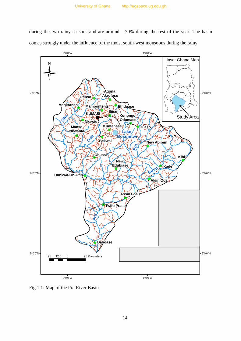
This study was carried out in the Pra River catchment which is located between latitudes

5º00׀N and 7º15

׀N and longitudes 0º03

׀W and 2º80

׀W (Fig.1.1). It is one of the south-western

drainage basins in Ghana. The Pra is the largest of the four principal rivers that drain the area

south of the Volta divide and enters the Gulf of Guinea east of Takoradi. Its main tributaries

are the Ofin, Oda, Anum and Birim rivers which drain from the Mampong-Kwahu Ranges.

The drainage basin area is 23,188 km2 with a mean annual discharge of 214 m

3s

-1 (Akrasi and

Ansa-Asare, 2008). The landscape is generally flat characterised by undulating topography

with an average elevation of about 450 m above sea level.

The main soil type of the catchment is forest ochrosols which are alkaline. The soils are

weathered from the Tarkwaian geological formations composing of sandstones and granitoids

and metamorphosed rocks such as phyllites and schists. The soils are clayey and not well

leached; hence have the capacity to retain more moisture and are very cohesive (Dickson and

Benneh, 1985).

The basin falls within the wet semi-equitorial climatic belt which is characterized by two

rainfall maxima, the first season is from May – June with the heaviest rainfall in June and the

second rainy season is from September – October. Relative humidities are highest (75-80%)


14

during the two rainy seasons and are around 70% during the rest of the year. The basin

comes strongly under the influence of the moist south-west monsoons during the rainy

Fig.1.1: Map of the Pra River Basin

"

!.

!.

!.

!.!.

!.!.

!.!.

!.

!.!.

!.!.

!.!.

!.

!.!.

!.

!.!.

Lake Bosumtwi

Ofin

Oda

Pra

Birim

Pra

Kibi

Kade

Ejisu

Juaso

Ofinso

Nkawie

Bekwai

Obuasi

Daboase

Akim Oda

EffiduaseMankranso

Kuntenase

Mamponteng

New Abirem

Assin Fosu

Twifo Praso

New Edubiase

MansoNkwanta

Agona Akrofoso

Dunkwa-On-Ofin

Konongo-Odumase

KUMASI

1°0'0"W

1°0'0"W

2°0'0"W

2°0'0"W

7°0'0"N 7°0'0"N

6°0'0"N 6°0'0"N

5°0'0"N 5°0'0"N

Ü

Legend

!. District Capital

" Regional Capital

River

Railway

Road

Lake

Watershed

25 0 2512.5 Kilometers

Inset Ghana Map

Study Area

Data Source: Ghana Survey DepartmentComposer: J.M. Kusimi - 2011.


15

season with high annual rainfall amounts of between 125 and 200 cm. Dry season is well

marked and spans from November to March. Temperatures are high throughout the year with

the highest mean monthly temperature being 30° C occurring between March and April and

the lowest is about 26° C in August (Dickson and Benneh, 1995).

The Pra Basin is covered by the moist-semi deciduous forest vegetation which contains

most of the Ghana’s valuable timber trees. The climatic environment of high temperatures

and heavy rainfall promote the rapid growth of trees particularly in the rainy season. Trees

grow to heights of about 35-45 m or more and are of three layers, the upper, middle and

lower layer. A typical semi-deciduous forest consists of trees, lianas, climbers and

shrubs/bushes which cover the soil from erosion by rain drops and run-off. However in the

dry season, certain species of the upper and middle layers shed their leaves during the long

dry spell. Due to the rapid expansion of the cocoa industry in this zone very little of the

original forest remains and most of what is left is secondary growth. The size of trees in this

belt therefore depends on how long the forest has been allowed to regenerate. Near large

settlements where the pressure on land is very great, fallow periods may be as short as 3

years, thus the vegetation is reduced to climbers, shrubs/short woody plants and grass species

interspersed by isolated tall trees left on the landscape by farmers (Dickson and Benneh,

1995).

The Pra Basin serves as the source of water supply for both industrial and domestic uses for

three regional capitals, 41 districts and over one thousand three hundred towns. Of the 41

administrative districts 20 are in the Ashanti Region, 11 in the Eastern Region, 6 in the

Central Region, and 4 in the Western Region. The Ofin sub-basin is the main source of water

supply to Kumasi and its environs, through two reservoirs, namely Barekese and Owabi

dams. The Birim sub-basin is located predominantly in the Eastern Region and has attractive

historic places and nine forest reserves. For instance, the Esen Epan Forest Reserve near


16

Akim-Oda is a tourist site with the biggest tree in West Africa at 12 m in circumference and

66.5 m tall. The major tributaries are perennial and constitute all-year-round reliable water

source. However, human activities such as mining, logging etc. are having adverse impacts

and degrading the surface water resources of the basin (Ghana Survey Department; Water

Resources Commission, 2011).

The Pra Basin is one of the most extensively and intensively used river basin areas in

Ghana in terms of settlement, agriculture, logging and mining due to its rich economic tree

species, rich mineral ore deposits and conducive environment for farming. The basin contains

most of the large cocoa growing areas in the Eastern, Ashanti, and Central regions. Tree cash

crop cultivation other than cocoa is mainly oil palm. Food cropping is increasingly becoming

more commercialized especially around the medium and large settlements and along the

major road arteries. The basin contains the highest density of settlements (both rural and

urban) in Ghana. It has a high concentration of mining activities mainly concerned with gold

and other minerals. Several large scale mining companies in the basin include AngloGold

Ashanti, Perseus Mining Ltd, Newmont Ghana Gold Ltd etc (Water Resources Commission,

2011).

The vegetative cover of the basin is experiencing rapid rate of deforestation due to human

activities such as farming, illegal small scale mining and lumbering (saw mills and chain-saw

operators) and this is hampering water resources management of the basin. Forest cover

outside the reserve areas is negligible and is estimated at less than 2% of the Basin. These

forests are heavily logged by both licensed timber firms and illicit loggers. These

anthropogenic activities are negatively impacting on the hydrological and geomorphological

processes within the basin. The implication of these human activities is sediment transport

into the river and channel morphological dynamics. The extensive forest clearance for

mining, settlement, and infrastructural development causes considerable loss of soil minerals


17

and subsequent high sediment transport in the Pra and its tributaries silting up channels and

dams (Water Resources Commission, 2011). Large scale and small scale mining with

disruptive impact on surface cover including soils occur around Obuasi, Kibi, Dunkwa-on-

Ofin, Konongo and most other communities within the basin. Moderate to severe sheet and

gully erosion poses a threat for flooding within the basin. For instance in July 2011, the Pra

and Birim rivers flooded their banks in the upper and middle courses where these

anthropogenic activities are intense destroying lives and property (Bentil, 2011).

1.5. Structure of the thesis

This thesis is organized into seven chapters. The first chapter gives background information

on fluvial geomorphology and the underpinning issues that are of focus by scientists. This

chapter also discusses the problem under study, questions that the study seeks to address and

outlines the objectives and hypotheses guiding the study. Lastly the chapter also introduces

the physical settings of the study area by stating the geographical position of the study area

and the underlying physical and socio-economic factors prevailing within the basin.

Chapter two encompasses literature review. The chapter reviews existing literature on

approaches for measuring/determining sediment yield, sediment sources and bank erosion in

fluvial geomorphology and other related fields such as hydrology, glacier geomorphology,

and oceanography, among others. The underlying processes involved in these landscape and

channel transformation and transportation of landscape materials are also reviewed. The

chapter also examines existing models for predicting sediment transport and sediment yield.

Chapters three to six are on the research methods and findings of each of the thematic set

objectives of the study. The last chapter is chapter seven and in this chapter, a general

discussion is done relating all the findings of the study, stating the significance of the results


18

to decision making and policy formulation, drawing conclusions and making

recommendations for future studies and for informed decision making.


19

Chapter Two

Literature Review

2.0 Introduction

The chapter reviews existing literature on approaches for measuring/determining sediment

yield, sediment sources and bank erosion in fluvial geomorphology and other related fields such

as hydrology, glacier geomorphology, and oceanography among others. The underlying

processes involved in these landscape and channel transformation and transportation of

landscape materials were also reviewed. The chapter also examines existing models for

predicting sediment transport and sediment yield. Informed by this existing literature, the

research methods and materials for the study were designed.

2.1 Stream Bank Erosion Processes and Measurements

Rivers perform three main sediment related activities; erosion, transportation and deposition.

These activities lead to the creation of erosional and depositional landforms (Nagle, 2000).

Materials are dislodged through the processes of abrasion and solution. Mass failure of river

banks due to the fluvial erosion at the toe banks also entrains materials into river channels. The

resultant impact of these fluvial processes is the formation of a myriad of fluvial landforms and a

change in the landscape in the long term. The morphology of catchment topography and river

channels depends to a large extent, on the interaction between hill slope and channel processes.

Consequently, many management theories, measurements and modelling have been developed in

order to reduce soil loss from basins and sediment transport to hydrologic drainage networks and

to explore the drainage basin structure and evolution (Amore, 2004; Tucker and Bras, 1998).


20

Stream bank erosion rate studies have been undertaken using conventional, manual and field

monitoring methods, and these involve erosion pins, cross section resurveys or terrestrial

photogrammetry (Lawler, 2005b; Billi, 2008; Bertrand, 2010). The conventional methods present

some significant disadvantages as they do not provide continuous measurements of fluvial

erosion, but instead provide snapshots of erosion between periods of measurements and do not

allow the accurate identification of the critical events triggering fluvial erosion (Bertrand, 2010;

Lawler et al., 1997).

New techniques available to estimate fluvial erosion rates or the erodibility parameters are the

jet testing device (Thoman and Niezgoda, 2008, in Bertrand, 2010), the LIDAR technology and

Airborne Laser Scanning (Korpela et al., 2009; Pizzuto et al., 2010; Thoma et al., 2005, in

Bertrand, 2010), and the Photo-electronic Erosion Pin (PEEP) (Bertrand, 2010; Lawler, 2005b;

Lawler et al., 1997). The advantage of the PEEP over the traditional methods is its ability to

continuously monitor bank retreat, which will better pinpoint the exact timing and magnitude of

small to moderate erosion events (Bertrand, 2010; Lawler, 2005b; Lawler et al., 1997). For

instance, Lawler (2005b) observed that, tidal banks are revealed to be much more dynamic using

PEEP measurements than previous conventional monitoring has indicated. Also, by comparing

PEEP to low-resolution monitoring of conventional methods, he indicated that, the frequencies

of low-resolution monitoring failed to adequately represent the cyclicity, mean, range, variability

and trend of bank elevation changes. However, PEEP is saddled with the problem of not being

able to record events at night. Also, some of these new methods are expensive for developing

countries. Erosion pin and cross sectional re-surveys methods are popular approaches as they are

cheap and easily operable (Bertrand, 2010).


21

2.2 Sediment Source Analytical Techniques

Determining the sources of sediments, and associated nutrients and contaminants, is an important

issue for the management of water quality in river systems (Caitcheon, 1998). Spatial sediment

tracing can be achieved by measuring the relative contributions of sediments and associated

substances at stream junctions, so that a budget of relative contributions for a whole drainage

network can be established (Caitcheon, 1998). In addition to spatial source tracing, dated

sediment cores from channel, floodplain deposits and reference inventories sampled at stream

junctions can provide valuable information about longer term trends in source contributions and

sediment erosion (Caitcheon, 1998; Matisoff and Whiting, 2011; Walling, 2004).

Symander and Strunk (1992, in Nagle et al., 2007) described some of the difficulties with the

use of suspended sediments to identify source areas. Two of the principal problems are the

enrichment of suspended sediments in fines and in organic matter relative to the sources and the

transformation of sediment properties within the fluvial system (Nagle et al., 2007). Recently

published work on the use of tracers, contend that the use of recent over bank deposits enables

the contributions of sediment sources to be identified more reliably and the long-term loading

from individual sources to be assessed (Bottrill et al., 2000, in Nagle et al., 2007).

Mapping erosional features in a watershed for sediment source tracking could involve using

photos, maps, field surveys, erosion pins and troughs. Assembling information on suspended

sediment sources has proved difficult using the traditional direct monitoring techniques (e.g.

erosion pins and troughs) due to inherent spatial and temporal sampling constraints and the

amount of fieldwork involved (Peart and Walling, 1988). Secondly, these traditional techniques

do not permit the derivation of the range of soil redistribution rates such as the mean erosion rate


22

for the eroding areas, the mean deposition rate for the depositional areas, the net soil loss from

the field and the sediment delivery ratio (Walling, 2004).

In response to the problems associated with traditional monitoring and measurement

techniques, the fingerprinting approach using tracers has been increasingly employed as a means

of establishing the relative importance of potential catchment sediment sources and soil erosion

rates (Collins et al., 1997; Collins et al., 2001; Mukundan et al., 2009; Nagle et al., 2007).

Sediment fingerprinting relies upon the premise that the physical and chemical properties of

suspended sediment will reflect its source (Collins et al., 1997; Collins et al., 2001). Another

fundamental condition that must be met by any tracer is that the tracer substance(s) must remain

unaltered within the spatial and temporal limits in which the tracing method is being applied,

(Caitcheon, 1998), adsorption of the tracer to soil is strong and quick; variation in adsorption to

various sizes or mineralogic/organic constituents is minor or can be accounted for (Matisoff and

Whiting, 2011).

The most commonly used tracers include; radionuclides (137

Cs, 210

Pb) (Nagle et al. 2007;

Walling, 2004), and cosmogenic isotopes (7Be) (Schuller et al., 2006; Walling, 2004).

137Cs has a

core depth profile not greater than 20 cm and is anthropogenically introduced into the

environment through fallouts of nuclear activities of bombs of 1950s and 1960s and reactors

such as the 1986 Chernobyl disaster. Lead-210 (t1/2 = 22years, with core depth of about 10 cm)

and beryllium – 7 (t1/2 = 53days and depth profile not exceeding 3 cm) are natural fallouts from

the atmosphere (Blake et al., 2002; Matisoff and Whiting, 2011), hence are ubiquitous on the

earth’s surface and thus are suitable as environmental radionuclides tracers everywhere. 137

Cs,

7Be, and

210Pb are each suitable as particle tracers because they have a global distribution, adsorb

efficiently to soil particles and thus move with soil, and are relatively easily measured (Matisoff


23

and Whiting, 2011). Also these environmental radionuclide tracer methods are effective for

distinguishing between surface-derived sediments from sheet and shallow rill erosion and

sediments from gullies and stream channel walls, because channel and gully walls deeper than

their profile depths of between 3 – 30 cm usually contain little or no traces of the radionuclides

(Nagle et al., 2007; Matisoff and Whiting, 2011). However, 137

Cs fallout from the atmosphere is

currently near zero or near non-detectable limits (Matisoff and Whiting, 2011) in most parts of

the world except northern Europe where release from the Chernobyl explosion was higher. Also

due to the short half life of 7Be, it is only suitable for simulating erosion of small catchments.

Other tracers include; stable isotopes (C-13, N-15) sediment carbon and nitrogen (Juracek and

Ziegler, 2009; Mukandaun et al., 2009), phosphorous (Wallbrink et al. 2003), clay mineralogy

(Youngberg and Klingeman, 1971; Glasmann, 1997, in Nagle et al., 2007), magnetic

susceptibility (Blake et al., 2006; Caitcheon, 1998; Gruszowski et al., 2003), and heavy metals

(Juracek and Ziegler, 2009) etc. In view of the multiplicity of elements being analyzed in these

approaches, they are often very costly hence not employed in most studies.

The fingerprinting technique could either be a simple mixing model using only one diagnostic

tracer or a composite mixing model involving a combination of two or more tracers. Some

researchers (Walling et al., 1993, Yu and Oldfield, 1989; Molinaroli et al., 1991) have, however,

argued that no single diagnostic property of sediment can reliably distinguish different sources,

because individual tracers may be subject to physical and chemical changes, which limit their

use, e.g. particle size sorting, organic matter selectivity, and geochemical transformation during

fluvial erosion and transportation (Collins et al., 1997). Also, individual properties may be

unreliable because of spurious source-sediment matches (Yu and Oldfield, 1989; Molinaroli et

al., 1991; Walling et al., 1993). For example, suspended sediment tracer values may resemble


24

those of a particular source, but could also result from various combinations of other sources

(Collins et al., 1997). However, Nagle et al., (2007) have effectively used a simple mixing model

of 137

Cs to distinguish between sediment from surface sources and gullies. Lead-210 (Brigham et

al., 2001; Motha et al., 2002) and Berryllium-7 (Schuller et al., 2006) have also been used

singularly in sediment source tracing. Sediment source tracking has also been performed

successfully in a subset of intermittent streams using amorphous to crystalline ratios of iron to

estimate the fraction of sediment coming from in-stream vs. landscape sources (Schoonover et

al., 2007). Parsons and Wainwright (1993) and Caitcheon (1998) used mineral magnetic

properties of sediments in tracing sediment sources.

The use of mixing and unmixing models of multi tracers involving multivariate statistics to

identify the relative contributions of surface erosion from different land use types and channel

erosion to suspended sediment load in river basins sources has also been demonstrated and

examined in detail in the literature (Collins et al., 1997; Collins et al., 2001; Gruszowski et al.,

2003). For instance Walling (2004) successfully used environmental radionuclides caesium-137,

lead-210, beryllium-7 to trace sediments mobilization and delivery in river floodplains in Devon,

UK. Though very effective and efficient in characterizing sediment sources and the redistribution

rates of sediments, the multi-tracer model approach is very complex, mathematical and very

demanding in terms of data, field work as well as laboratory logistics with huge financial burden.

Issues of sample size and the range of tracer properties that are measured have also being raised

(Gruszowski et al., 2003).

GIS and remote sensing techniques and other modelling programmes such as USLE, WEPP,

DR3M, WFPB, GWLF (Arekhi, 2008; Jain et al., 2010, Nangia et al., 2010; Mongkolsawat,

1994; Roy, 2009; Wahyunto and Abdurachman, 2010) have recently been employed for


25

sediment source tracking in catchments. Models are appealing because they are cheaper to use.

They are also most effective for source analyses where the models have been applied and

calibrated. Models are used by reviewing existing data, and consulting with those who are

familiar with basin conditions (Gellis, 2010). However with very large basins some models are

associated with large errors. Secondly, some are very complex and require very complex input

data sets such as the hydrology, rainfall interception by vegetation (e.g. throughfall, stemflow

etc), water balance, plant growth and residue decomposition of catchments which make them

unsuitable in the developing countries where such explicit data is difficult to generate (e.g.

WEPP and EUROSEM).

The latest modelling approaches to overcome the limitations of the empirical USLE

concentrate on physically based erosion models such as SWAT (Arnold et al. 1998; Gassman et

al., 2007, in Silva et al., 2010), Water Erosion Prediction Project (WEPP) (Amore et al., 2004)

and EUROSEM (Morgan et al., 1998). These are physically based models with the basic

processes incorporated in them so that they can simulate the individual components of the entire

erosion process by solving the corresponding equations; and so it is argued that they tend to have

a wider range of applicability (Amore et al., 2004; Silva et al., 2010). Such models are also

generally better in terms of their capability to assess both the spatial and temporal variability of

the natural erosion processes (erosion and deposition) (Amore et al. 2004). Though these models

are transferable to other watersheds, they require huge amounts of input data and many

calibration parameters, complex laboratory analyses or hard and expensive field data collection,

which are commonly out of reach of many developing countries (Renschler et al., 1999; Silva et

al., 2010).


26

2.3 Sediment Yield Measurements

Sediment yield is the amount of sediment load passing the outlet of a catchment, that is the

sediment load normalized for the drainage area and is the net result of erosion and deposition

processes within a basin (Jain and Das, 2010; Restrepo and Syvitski, 2006; Verstraeten and

Poesen, 2001). These materials are of three different kinds; dissolved load (consisting of soluble

materials carried as chemical ions); suspended load (containing clay and silt held up by the

turbulent flow), and bed load which includes larger particles moved by saltation, rolling and

sliding (Nagle, 2000).

However, on the basis of transport processes, measurement principles, and

morphological/sedimentary associations, fluvial sediments are often classified into two; bed

materials and washed materials. Bed material is often conflated with bed load (makes up the bed

and lower banks of the river channel), and wash material moves in suspension and travels out of

the reach once entrained (measured load), but the two classifications are not congruent (Church,

2006). Depending on discharge/flow rate, the medium grain sand particles (saltation materials)

could become unmeasured sediments if the popular Helley-Smith sampler is used. Generally, the

size of material that moves as bed or suspended load in the flow depends upon the power and

turbulence of the flow (Gomez and Church, 1989).

In relatively deep streams of high flows, with bed material that consists of fine sand, the

suspended bed material may be 90% or more of the total sediment discharge. However, in

shallow streams with medium to coarse sand beds, the unmeasured-sediment discharge may

represent 50% or more of the total sediment discharge (Andrews, 1981). Various approaches

have been developed to determine river sediment yield and these include field measurements and

modelling (physical and empirical). Suspended load and bedload are measured or estimated


27

separately because the physical processes that govern their rates of transport are dependent on

different factors. The sum of suspended load and bedload is the total sediment load (Edwards and

Glysson, 1999).

2.3.1 Field Measurements of Sediment Yield

Measuring and estimating suspended sediment yields in rivers has long been subject to confusion

and uncertainty (Thomas, 1985) because various methods have been developed to measure

suspended sediment yield and they include the measurement of suspended sediment load and

water discharge (Akrasi, 2005; Khanchoul et al., 2010; Kusimi, 2008), measuring total eroded

soil and deposited sediments in small catchments (Verstraeten and Poesen, 2001), and measuring

sediment volumes in ponds, lakes or reservoirs (Nichols, 2006; Verstraeten and Poesen, 2001).

For the measurement of sediment volumes in ponds, lakes and reservoirs, radiometric techniques

using 210

Pb or 137

Cs as tracer elements can be employed to reconstruct sediment budgets over a

period of time (Foster et al., 1990; Govers et al., 1996; Walling, 1990 cited in Verstraeten and

Poesen, 2001).

The ideal situation to estimate the suspended sediment yield of rivers would be to measure

suspended sediment concentration and water discharge continuously and use the product

function as an estimate of suspended sediment discharge (Lane et al., 1997; Thomas, 1985).

Obtaining continuous records of concentration however is practically impossible owing to cost,

number of samples and sampling frequency among others (Edwards and Glysson, 1999; Thomas,

1985). Alternative to these issues of cost, remoteness of sites, and technical difficulties is to

measure water discharge continuously and to take occasional discrete water samples either


28

manually or using automatic sampling equipment for gravimetric analysis of suspended sediment

concentration (Thomas, 1985).

The use of sediment-discharge rating curve to estimate sediment yield is however problematic

because suspended-sediment concentrations are known to be variable for a given discharge

because stormflow hydrographs usually, but not always, are characterized by higher suspended-

sediment concentrations during the rising limb than the falling limb. Further, the timing between

storm events also influences availability of fine-grained sediment from the watershed, such that

an initial stormflow following relatively dry conditions usually has a greater suspended-sediment

concentration than subsequent flows of similar magnitude (Edwards and Glysson, 1999).

Consequently, statistical considerations show that the sediment load of a river is likely to be

underestimated when concentrations are estimated from water discharge using least squares

regression of log-transformed variables (Asselman, 2000; Cohn et al., 1992; Ferguson, 1986;

Jansson, 1985; Singh and Durgunoglu, 1989). Also regardless of how the samples are collected,

there remain questions of when the measurements of concentration should be made, how they

should be used to estimate the total yield, how close can samples be spaced in time and still be

meaningful among others (Edwards and Glysson, 1999; Thomas, 1985).

According to Edwards and Glysson, (1999), spatio-temporal variations in sediment transport

can be captured by collecting depth/point-integrated suspended-sediment samples that define the

mean discharge-weighted concentration in the sample vertical and collecting sufficient verticals

to define the mean discharge weighted concentration in the cross section. Verticals of samples

could either be taken using Equal-Discharge-Increment or Equal-Width-Increment Methods.

Though both methods have their advantages and disadvantages, if properly used, they yield

similar results.


29

Also the biases in the estimation of sediment loads by rating curve due to using log-

transformed estimates can be significantly reduced by using nonlinear regression. Further

improvements can be achieved by identifying seasonalities and breaks in slopes of the rating

curves and taking samples at the right time. Finally, the underestimation caused by using average

daily flows with the rating curve can be eliminated by using sub-daily flow data, if available

(Singh and Durgunoglu, 1989). The many methods that have been developed for collecting data

and estimating suspended sediment yields indicate each method is characterised by one

limitation or the other, thus the method that one employs is subject to availability of equipment,

cost, convenience, the kind of results that is sought among others.

2.3.2 Sediment Yield Modelling

Sediment yield and surface erosion at a watershed or regional scale are at present also modelled

using empirical models such as the universal soil loss equation (USLE), modified universal soil

loss equation (MUSLE) or the revised universal soil loss equations (RUSLE and RUSLE 2)

which are sometimes integrated into GIS (Arekhi, 2008; Jain et al., 2010; Mongkolsawat, 1994;

Nangia et al., 2010; Roy, 2009; Wahyunto and Abdurachman, 2010). Others include WEPP,

SWAT, EUROSEM etc (Amore et al., 2004; Fistikoglu and Harmancioglu, 2002).

Universal Soil Loss Equation (USLE) and its revised versions (RUSLE and RUSLE2) have

been used to model soil erosion sometimes integrating the parameters of the model in GIS to

produce soil erosion risk maps (Bonilla et al., 2010; Fistikoglu and Harmancioglu, 2002; Kouli et

al., 2008; Silva 2004; Silva et al., 2010; Stone and Hilborn, 2000; Roy, 2009; Wahyauto, 2010).

The USLE/RUSLE though empirical without spatial dimensions like some of their counterparts,

they are however simple and their parametric data can easily be transformed into GIS input data


30

formats for spatial analysis of phenomena. Secondly, their data requirements are not too complex

and literature has shown that they have been successfully used to estimate soil erosion of

catchments and farmlands (Arekhi, 2008; Fistikoglu and Harmancioglu, 2002; Jain and Kothyari,

2000; Jain and Das, 2010; Jain et al., 2010; Silva et al., 2010).

However, USLE/RUSLE only predicts the amount of soil loss that results from sheet or rill

erosion on a single slope and does not account for soil losses from gully, wind or tillage erosion

and deposition (Stone and Hilborn, 2000). Consequently, RUSLE was subsequently revised to

include more advanced scientific interface as RUSLE 2 which permits the segmentation of

topography to determine sediment yield and deposition based on changes in topography, soil and

management systems along a flow path (Dabney et al., 2011; Stone and Hilborn, 2000; USDA-

ARS, 2008a, 2008b). Despite these advancements, RUSLE2 cannot predict erosion within

concentrated flow channels (gulley erosion) (Dabney et al., 2011; USDA-ARS, 2008a). Also,

RUSLE2 is too rigorous with a lot of data requirements some of which do not have spatial

domain (e.g. surface roughness, sediment detachment, sediment transport and sediment

deposition models) and as such cannot be analysed with GIS. Though it has a higher

predictability of soil erosion than USLE/RUSLE, it is only applicable to small farm plots hence

inappropriate for large river catchments like the Pra River Basin.

The other models (e.g. WEPP, SWAT, EUROSEM, MIKE SHE, ANSWERS, CREAMS etc)

are applicable at catchment scale, event based, continuous models spatially and temporally

distributed (i.e. 2D) (e.g. Amore et al., 2004; Fistikoglu and Harmancioglu, 2002). As already

discussed above, these models require substantial data inputs, many calibration parameters,

characterized by complex laboratory analyses or hard and expensive field data collection (Silva


31

et al., 2010) and thus are inappropriate to apply in developing countries where physical data on

river basins are non-existent or very limited.

2.4 Soil Erosion and Sediment Yield Modelling

In order to improve water quality and restore impaired watersheds, managers need to make

decisions using data that they are able to gather (Nangia, 2010). Data collection can be

expensive, tedious and time consuming, so in such situations using modelling approach makes

sense (Nangia, 2010) particularly in the developing countries where institutions and

organizations charged with the monitoring and collection of data are ill-equipped in terms of

personnel, materials as well as financial. Models for sediment yield provide invaluable

information when applied to those areas lacking data, for predicting future impacts of

agricultural activities, land use, stream stabilization and sediment storage in reservoirs

(Khanchoul et al., 2010). The revised universal soil loss equation has been widely used with very

good results, is applicable in a GIS environment and so can provide a spatial distribution of

erosion and soil loss, requires a small and simple input data set, is relatively easy to use and is

suitable for the study, thus its structure and operating system are being discussed for clarity.

2.4.1 The Revised Universal Soil Loss Equation (RUSLE)

A first attempt to evaluate and quantify the human impact on soil erosion such as land use

changes or new cultivation techniques was the universal soil loss equation (USLE) developed by

Wischmeier and Smith (1958) (Renschler et al., 1999). Since then, modified versions such as the

revised universal soil loss equation (RUSLE) (Renard et al., 1991), modified universal soil loss

equation (MUSLE) (Blaszczynski, 2003) have been widely used as tools for predicting soil


32

erosion in many parts of the world (Renschler et al., 1999). USLE, RUSLE and MUSLE were

defined by the following equation whose variables were annually estimated (Wischmeier and

Smith 1978):

A =R x K x LS x C x P ……………… (2.1),

where A represents the potential long term average annual soil loss in tonnes per hectare per

year; R is the rainfall erosivity factor (MJ mm ha/h/yr); K is the soil erodibility factor (t h MJ-1

mm-1

); LS is the slope length-gradient factor, C is the crop/vegetation and management factor,

and P is the support practice factor and these other parameters are all dimensionless.

The rainfall erosivity index (r factor) measures the potential ability of rain to cause soil

erosion. The R-factor is the sum of individual storm erosivity index (EI)-values for a year

averaged over long time periods (> 20 years) to accommodate apparent cyclical rainfall patterns.

Storm erosivity (EI = r) is the product of a storm’s total energy (E) and its maximum intensity (I)

within a stipulated time frame which in standard time could be 5 min, 10 min, 15 min, 30 min,

60 min etc (Renard and Freimund 1994; USDA-ARS, 2008a). An erosive event is a rainfall

event with more than 12.50 mm of total rainfall accumulation or with at least 6 mm of rainfall

accumulation in 15 minutes (Petkovšek and Mikoš, 2004; USDA-ARS, 2008a). The three most

common mathematical models used to relate the kinetic energy (KE) to rainfall intensity are the

logarithmic model, exponential model, and the Hudson (1965) model (Shamshad et al., 2008).

The original method for calculating R values for a storm event requires pluviograph records

(Table 2.1) (Wischmeier and Smith, 1978). This kind of information is difficult to obtain in

many parts of the world because its processing is time-consuming, labour-intensive, and costly

(Eltaif et al., 2010; Silva, 2004). There is also a lack of pluviograph record data in most

developing countries. The successful use of the EI30 in certain temperate regions (such as its


33

place of origin) does not guarantee its success as an index of soil loss in regions with

substantially different climates, such as the tropics, because erosive rainfall in the tropics differs

from that in other regions mainly in intensity and frequency characteristics (El-Swaify et al.,

1982).

A number of indices which relate the erosivity of a rainstorm and its associated runoff to soil

loss prediction have been established. The most commonly used indices include the Founier

Index (Fournier, 1960), the modified Founier Index (MFI) (Arnoldus, 1980), Hudson’s KE > 25

Index (Hudson, 1965), Lal’s AIm, Index (Lal, 1976) and the erosivity index (EI30) of the

Universal Soil Loss Equation (Renard and Freimund, 1994; Vrieling et al., 2010; Wischmeier

and Smith, 1978). In the US, the R-factor can be evaluated or calculated using methodological

guides of Wischmeier and Smith (1978). In contrast, lack of rainfall intensity data in some

countries makes the calculation of R-factor, especially in the developing world, very difficult.

Although the most accurate estimate of R-values can only be obtained from longterm rainfall

intensity data as calculated by Wischmeier and Smith (1978), several works suggest that monthly

precipitation data can give reasonable estimates of R-values for many regions throughout the

world (Renard and Freimund, 1994; Shamshad et al., 2010; Vrieling et al., 2010). Several

authors have derived exponential/regression relationships between R and average monthly

precipitation of the wettest month. Also, R is well correlated with the modified Fournier index

(Table 2.1). Although very useful for estimating relative erosion hazards, mean annual rainfall is

not directly correlated with soil loss in the tropics due to differences in rainfall characteristics

and vegetative cover, hence the use of rainfall amounts in deriving R factor is over simplification

of soil erosion process (El-Swaify et al., 1982). For example, erosivity index varies from 50 to

650 in the United States, 60 to 300 in Tunisia, 50 to 300 in Morocco, 60 to 340 in the South of


34

France, and 500 to1400 in Ivory Coast (Roose, 1977). The works of these scientists indicate that

an erosivity variable may be dependent on the climatic conditions of the geographical area, scale

of the study area, and type of measurement and that there is no single universal variable better

than the others (Irvem et al., 2007, Renard and Freimund 1994; Stocking, 1987).

Table 2.1: Examples of models for the derivation of R values

(EI30)i is EI30 for storm i, j no. of storms in an N year period, ρ the average rainfall (mm) of the month with the

highest rainfall, P the average annual rainfall (mm), F the modified Fournier Index, H rainfall

amount, Pi monthly precipitation of month i , Pei effective monthly precipitation of month i, Pt

annual rainfall amount (mm), I30 maximum intensity in 30 minutes. (Angulo-Martínez and

Beguería 2009; Diodato and Bellocchi, 2007).

Soil erodibility factor (K) is the average soil loss in tonnes/hectare for a particular soil in

cultivation under continuous fallow on a plot with a slope length of 22.13 m and slope steepness

of 9%. K is a measure of the susceptibility of soil particles to detachment and transport by

rainfall and runoff (Stone and Hilborn, 2000). The LS factor represents a ratio of soil loss under

given conditions to that at a site with the “standard” slope steepness of 9% and slope length of

22.13 m. The steeper and longer the slope, the higher is the risk for erosion (Stone and Hilborn,

2000). Slope length has been defined as the distance from the point of origin of overland flow to

Number Equation Author

1 R =

,

Wischmeier and Smith, 1978

2 R = 0.04830P1.610

Renard and Freimund 1994

3 R = 587.8 - 1.219P + 0.004105P2 Renard and Freimund 1994

4 R = 0.07397F1.847

Renard and Freimund 1994

5 R = 95.77 - 6.081F + 0.4770F2 Renard and Freimund 1994

6 FI or R = ρ2/P Vrieling et al, 2010

7 MFI or R =

De Luis et al (2010)

8 MFIe or R =

Smithen and Schulze (1982).

9 R = 0.577H - 5.766 Roose, 1977

10 R = (0.0158H x I30) - 1.2 Roose, 1977

11 EI30 = 227MFI0.548

Shamshad et al, 2010


35

the point where either the slope gradient decreases enough that deposition begins or the flow is

concentrated in a defined channel (Wischmeier and Smith, 1978). Traditionally estimates for L

were obtained from field measurements, however, this method requires high financial and human

resources which are not feasible at regional scale (Van Remortel et al., 2001; Hickey et al.,

1994). With advancement in computers, there are several algorithms that have been packaged

into GIS softwares that make the derivation of slope length and steepness simpler. These include

using either unit stream power (Moore and Burch, 1986) or upslope area (Desmet and Govers,

1996) as a surrogate for slope length, the neighbourhood method and the best fit plane method

(Srinivasan and Engel, 1991), grid-based methods and the maximum downhill slope angle

(Hickey et al., 1994; Hickey, 2000; Van Remortel et al., 2001), network triangulation (Cowen,

1993) techniques (cited by Hickey, 2000), quadratic surface, maximum slope and maximum

downhill slope techniques (Van Remortel et al., 2001). Among these, the one that is best suited

for integration with GIS is the theoretical relationship proposed by Moore and Burch (1986) and

Moore and Wilson (1992) based on unit stream power theory, given as (Jain and Das, 2010; Jain

and Kothyari, 2009; Silva et al., 2010):

……………… (2.2)

where As is the specific area (=A/b), defined as the upslope contributing area for an overland cell

(A) per unit width normal to the flow direction (b); is the slope gradient in degrees.

The cover management factor C is used to determine the relative effectiveness of soil and crop

management systems in terms of preventing soil loss. The C factor is a ratio comparing the soil

loss from land under a specific crop and management system to the corresponding loss from

continuously fallow and tilled land (Stone and Hilborn, 2000). The support practice factor P

reflects the effects of practices that will reduce the amount and rate of the water runoff and thus


36

reduce the amount of erosion. The P factor represents the ratio of soil loss by a support practice

to that of straight-row farming up and down the slope. The most commonly used supporting

cropland practices are cross slope cultivation, contour farming and strip cropping (Stone and

Hilborn, 2000).

The genesis of RUSLE is USLE (Universal Soil Loss Equation) introduced in 1958 by W. H.

Wischmeier and D. D. Smith with the U.S. Department of Agriculture (USDA), Agricultural

Research Service (ARS), Soil Conservation Service (SCS), and Purdue University. USLE was an

empirical model of simple structure that captured the main effects of rainfall intensity, soil type,

topography, and management on sheet and rill erosion, with no attempt to account for sediment

deposition nor gully erosion (Dabney et al., 2011; Renard et al., 1991). USLE only predicts the

amount of soil loss that results from sheet or rill erosion on a single slope and does not account

for additional soil losses that might occur from gully, wind or tillage erosion (Stone and Hilborn,

2000).

In the early 1980s a programme to develop technology to replace the USLE was initiated,

resulting in the computer-based revised universal soil loss equation (RUSLE) model,

documented in written form in 1997 (Renard et al., 1997, cited by Dabney et al., 2011). RUSLE

incorporated significant advances over the USLE and this permitted the application of soil

erosion estimation for a great variety of crops and management practices beyond those in the

original USLE data base. Some other changes include a sub factor method for computing values

for the cover-management factor, improved factor values for the effects of contouring, terracing,

strip cropping, and management practices for rangeland (Dabney et al., 2011; Renard et al.,

1991; Stone and Hilborn, 2000). In addition, RUSLE introduced new slope length and steepness

(LS) algorithms reflecting rill to inter-rill erosion ratios and the capacity to calculate LS products


37

for slopes of varying shape (Renard et al., 1991; Stone and Hilborn, 2000) and thus is a better

estimate of soil erosion and sediment yield in landscapes than USLE.

2.5 Justification for Research Methodologies

Many published soil loss and sediment yield models, sediment yield, bank erosion and sediment

source tracking approaches were reviewed to understand their techniques and applications.

Relative merits and shortcomings of these methodological approaches in soil erosion and

sediment yield studies were discussed. It was realised that there is no universally acceptable

method or approach to modelling a catchment's soil erosion and sediment yield as well as field

data collection of sediment discharge measurements. The choice of any methodology depends on

the availability of resources (secondary data, financial, equipment etc) at the disposal of the

researcher.

However, for soil erosion and sediment yield modelling, the literature showed that, RUSLE has

been widely used with very good results, is applicable in a GIS environment and so can provide a

spatial distribution of erosion and soil loss in catchments. The model also requires a small and

simple input data set and is relatively easy to use and thus suitable for this study. Hence, the

RUSLE model was chosen to model soil erosion and sediment yield in the basin. However, a

slight modification to the model was made. Due to the high intensity of tropical rains as

compared to temperate regions, two rainfall erosivity events were adopted; the standard 12.5mm

erosive event and then 12mm event, to see whether a lower rainfall event will have any

significant impact on soil erosion and sediment yield in the basin. The thunderous tropical

raindrops (high intensity and large rain drops) will have more destructive impact on soil

aggregates as compared to temperate raindrops, hence the need to examine this effect. For


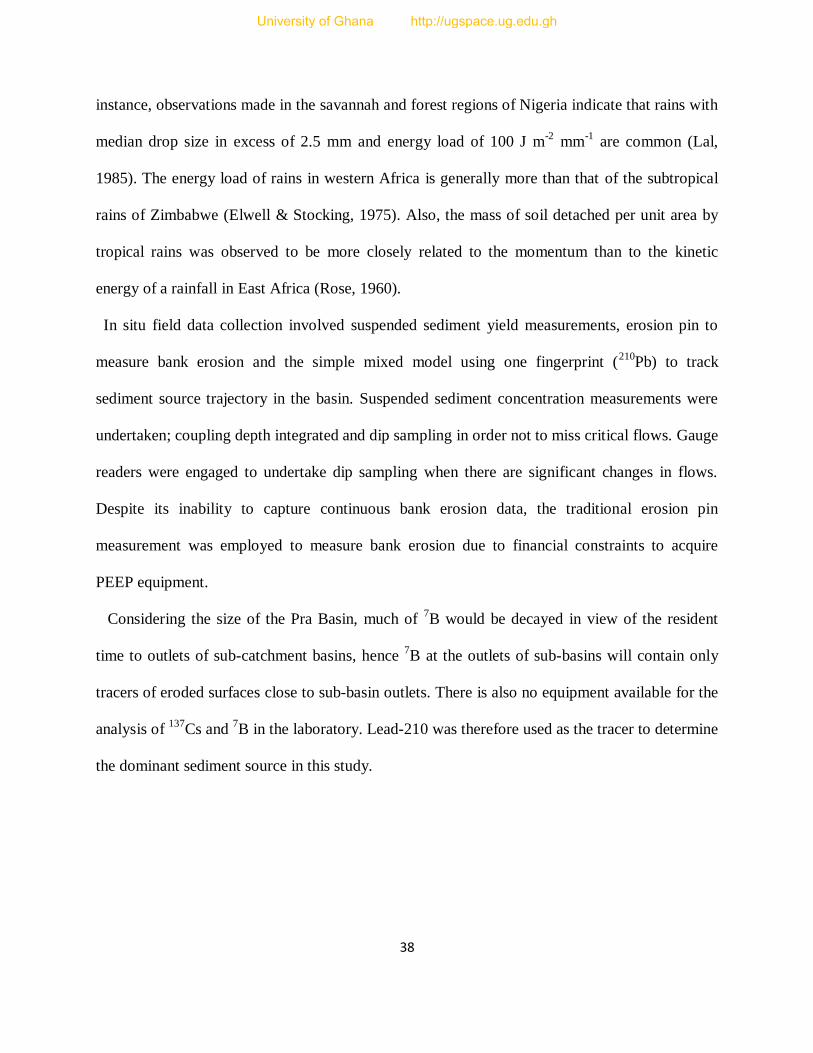
38

instance, observations made in the savannah and forest regions of Nigeria indicate that rains with

median drop size in excess of 2.5 mm and energy load of 100 J m-2

mm-1

are common (Lal,

1985). The energy load of rains in western Africa is generally more than that of the subtropical

rains of Zimbabwe (Elwell & Stocking, 1975). Also, the mass of soil detached per unit area by

tropical rains was observed to be more closely related to the momentum than to the kinetic

energy of a rainfall in East Africa (Rose, 1960).

In situ field data collection involved suspended sediment yield measurements, erosion pin to

measure bank erosion and the simple mixed model using one fingerprint (210

Pb) to track

sediment source trajectory in the basin. Suspended sediment concentration measurements were

undertaken; coupling depth integrated and dip sampling in order not to miss critical flows. Gauge

readers were engaged to undertake dip sampling when there are significant changes in flows.

Despite its inability to capture continuous bank erosion data, the traditional erosion pin

measurement was employed to measure bank erosion due to financial constraints to acquire

PEEP equipment.

Considering the size of the Pra Basin, much of 7B would be decayed in view of the resident

time to outlets of sub-catchment basins, hence 7B at the outlets of sub-basins will contain only

tracers of eroded surfaces close to sub-basin outlets. There is also no equipment available for the

analysis of 137

Cs and 7B in the laboratory. Lead-210 was therefore used as the tracer to determine

the dominant sediment source in this study.


39

Chapter Three

Sediment Concentration and Yield Measurement in the Pra Basin

3.0 Introduction

Information on sediment yield of a river basin is an important requirement for water resources

development and management (Akrasi, 2011), because high sediment loads affect water quality

and silt reservoirs. However, data on fluvial sediment are very limited because it is very

expensive to collect such data and also for lack of logistic support (Amisigo and Akrasi, 1998;

Akrasi, 2005). The amount of sediment yield generated within a catchment is a function of a

number of anthropogenic and physical factors including farming, mining, construction, slope,

basin area and rainfall intensity. This chapter presents methods and results of sediment yield

measurements undertaken in selected sampling stations within the Pra Basin to ascertain

sediment discharge levels and derived rating curves for the stations.

3.1 Research Materials and Methods

To determine the annual temporal variability in sediment yield for the year, fluvial sediment

samples were collected from March (low flows at the beginning of the rainy season) to

December at the end of the season at 7 monitoring stations (Fig.3.1) as suspended sediment

concentration in streams can change appreciably over seasonal timescales and during high flow

events (Lawler et al., 2006a). In order not to miss critical flows, gauge readers were engaged

where possible to take dip samples when there were significant changes in gauge heights. Dip

samples were taken simultaneously alongside depth-integrated samples during field visits and

correlated with the integrated samples to obtain a correction factor which was used to adjust dip


40

Fig.3.1: Sediment Yield Sampling Stations

"

"

"

"

"

" "

"

"

Lake Bosumtwi

Ofin

Oda

Pra

Birim

Pra

Anwiankwanta

Akim Oda

Adiembra

Assin Praso

Twifo Praso

Sekyere Heman

Brenase

1°0'0"W

1°0'0"W

2°0'0"W

2°0'0"W

7°0'0"N 7°0'0"N

6°0'0"N 6°0'0"N

5°0'0"N 5°0'0"N

Ü

10 0 105 Kilometers

Inset Ghana Map

Study Area

" Sediment Yield Sampling Sites

River

Watershed

Lake

Legend


41

samples taken by gauge readers (e.g. Akrasi, 2011; Edwards and Glysson, 1999). To account for

lateral and vertical variability in sediment concentration, sampling was cross sectional (equal-

width-increment) using the depth-integrated sampler as sediment varies vertically and laterally

within the river channel. Samples were taken at the midpoints of intervals (Edwards and

Glysson, 1999). In the absence of a bridge at Sekyere Hemang, dip samples were taken across

the channel in a canoe. At gauged stations, gauge heights were read when sampling. The

suspended sediment samples were analyzed in the Ecological Laboratory at the Department of

Geography, University of Ghana, Legon, using the evaporation method.

Suspended sediment samples were flocculated using magnesium chloride (MgCl2), allowed to

settle for 24 hours, and the supernatant decanted (e.g. Kusimi, 2008; Schoonover, 2007).

Sediments at the bottom of the container were emptied into dishes of known tare weights and

oven dried at 85○C (e.g. Di Stefano et al. 2000; Kusimi, 2008). The gross weights of the glass

dishes were taken after cooling in a desiccator. The tare weights of dishes were deducted from

gross weights to obtain sediment weight of each sample (e.g. Sengtaheuanghoung et al., 2007).

The weight of each sediment was divided by the weight of the water-sediment mixture and then

multiplied by one million converting it to parts per million to obtain suspended sediment

concentration of the sample (Porterfield, 1972). Samples at each point interval were added to

determine mean sediment concentration for that cross section in milligrams per litre.

The daily suspended sediment discharge/sediment load was computed using instantaneous

concentration and flow equation;

L = 0.0864CQw, ………………………… (3-1)


42

where, L = sediment load in tonnes/day; 0.0864 = conversion factor assuming a specific weight

of 2.65 for sediment; C = instantaneous concentration/sediment concentration, in mg/l; and Qw =

instantaneous water discharge, in m3/s (Osten, 1979; Yüksel et al., 2008).

Water discharge at gauged stations was derived using water discharge rating curves (Table 3.1)

whiles at ungauged stations (i.e. Assin Praso and Anwiankwanta) flow measurements were

undertaken using the current meter and float methods to determine water discharge. The float

method was employed during high flows and current meter when flows were low. Equations for

the water discharge rating curves were obtained from the Hydrological Services Department -

Accra. A water discharge rating curve was derived for Anwiankwanta using the log transform

power function (Table 3.1).

Table 3.1: Discharge Rating Curves

No. Station Equation Source

1 Sekyere Hemang Qw = 45.14(h – 0.2)1.93

Hydrological Services

Department - Accra

2 Twifo Praso Qw = 16.56(h + 0.09)2.64

׀ ׀

3 Akim Oda Qw = 10.47(h – 0.46)1.45

׀ ׀

4 Adiembra Qw = 6.79(h – 0.37)1.6

׀ ׀

5 Praso-Brenase Qw = 6.14(h – 0.42)1.57

Hydrological Services

Department - Accra

6 Anwiankwanta Qw = 3.468h1.7968

Author – Fieldwork, 2012

NB: h is gauge height

Sediment rating curves were then derived from graphical plots of the daily water discharges

and the daily cross sectional mean suspended sediment discharges. The sediment rating curves

are derived using a log transformed power function equation in the form (Achite and Ouillon,

2007; Asselman, 2000; Khanchoul et al., 2010);

Qs = aQb.................... (3-2);

where Qs is the daily mean suspended sediment discharge in t day-1

, Q is the daily mean water

discharge in m3s

-1, and a and b are constant and exponent of the rating curve.


43

Mean monthly sediment load and yield, annual suspended sediment yield and annual specific

sediment yield for the period were derived from the daily sediment discharge data of the

monitored stations. Mean monthly suspended sediment load is an average of the daily sediment

discharge per month (t day-1) whiles the monthly sediment yield was determined by multiplying

mean monthly suspended sediment load by number of days of the month (t/month). Annual

suspended sediment yield is the sum of monthly sediment yield for the year (t/yr-1

). The annual

specific sediment yield was obtained by dividing annual suspended sediment yield by catchment

area (t km-2

year-1

) (e.g. Akrasi, 2011; Akrasi, 2005).

3.2 Results and Discussion

Trends in the daily mean sediment concentration are shown in Figs.3.2 – 3.8. Generally sediment

concentrations in all stations have been fluctuating staggered by series of sharp rises and declines

in concentration amounts from March to December. At Anwiankwanta the lowest concentration

109 mg/l was observed in November and at Brenase it was about 106 mg/l in March with the

highest concentrations occurring in October at Anwiankwanta (869 mg/l) and June at Brenase

(1216 mg/l) (Figs. 3.2 and 3.3). There was a sharp rise in sediment concentration at the

beginning of the rainy season at Akim-Oda reaching 652 mg/l in May and thereafter, there was a

gradual decline to below 750 mg/l at the beginning of August. From August however,

concentration amounts rose again reaching 736 mg/l which was the highest for the year and

declined from this month onwards till the end of the year (Fig.3.4). At Adiembra maximum

sediment concentration 295 mg/l was also recorded in August whereas the minimum

concentration 44 mg/l was in November (Fig.3.5). At Twifo Praso there was a dip in sediment

concentration from 992 mg/l at the beginning of the year to about 357 mg/l in July followed by a


44

rise to nearly 1500 mg/l in September (Fig.3.6). At Assin Praso and Sekyere Heman, there was a

gradual rise in sediment concentration from March, peaking in September at Assin Praso and

Fig.3.2: Daily mean concentration of samples at Anwiankwanta

Fig.3.3: Daily mean concentration of samples at Brenase

0

100

200

300

400

500

600

700

800

900

1000

24 M

22 M

18 J 20 J 22 J 29 J 10 J 22 J 3A 6 S 16 O

19 O

21 O

23 O

28 O

30 O

8 N 16 N

25 N

28 N

9 D

Dai

ly m

ean

co

nce

ntr

atio

n (

mg

/l)

Sampling days (2012)

0

200

400

600

800

1000

1200

1400

21 M

29 A

7 M

24 M

15 J

16 J

1 J

3 J

12 J

13 J

14 J

16 J

20 J

6A

11A

17 A

19 A

22 A

28 A

3 S

7 S

12

S

17

S

29

S

1 O

3 O

5 O

23

0

11

D

Dai

ly m

ean

co

nce

ntr

atio

n (

mg

/l)



45

Fig.3.4: Daily mean concentration of samples at Akim Oda

Fig.3.5: Daily mean concentration of samples at Adiembra

0

100

200

300

400

500

600

700

800

22 M 28 A 22 M 15 J 19 J 11 J 12 J 1A 2A 17 A 4 S 29 S 2 O 23 O 15 N 11 D

Dai

ly m

ean

co

nce

ntr

atio

n (

mg

/l)


0

50

100

150

200

250

300

350

24 M

27 A

19 M

21 M

23 M

16 J 18 J 18 J 19 J 19 J 20 J 20 J 21 J 10 J 2A 3A 3A 19 A

6 S 30 S

26 O

17 N

9 D

Dai

ly m

ean

co

nce

ntr

atio

n (

mg

/l)



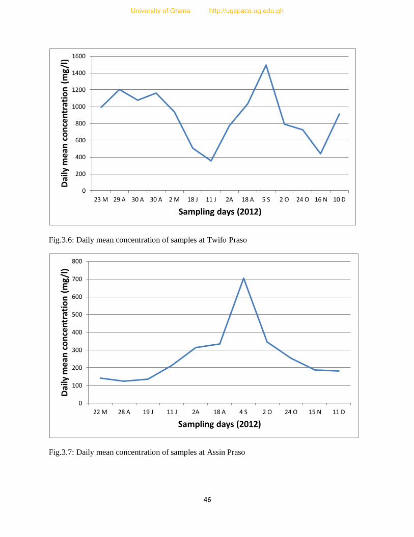
46

Fig.3.6: Daily mean concentration of samples at Twifo Praso

Fig.3.7: Daily mean concentration of samples at Assin Praso

0

200

400

600

800

1000

1200

1400

1600

23 M 29 A 30 A 30 A 2 M 18 J 11 J 2A 18 A 5 S 2 O 24 O 16 N 10 D

Da

ily m

ean

co

nce

ntr

atio

n (

mg

/l)


0

100

200

300

400

500

600

700

800

22 M 28 A 19 J 11 J 2A 18 A 4 S 2 O 24 O 15 N 11 D

Dai

ly m

ean

co

nce

ntr

atio

n (

mg

/l)



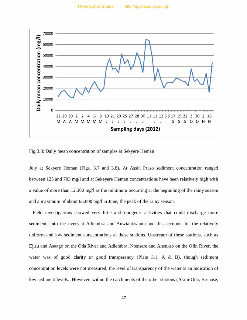
47

Fig.3.8: Daily mean concentration of samples at Sekyere Heman

July at Sekyere Heman (Figs. 3.7 and 3.8). At Assin Praso sediment concentration ranged

between 125 and 703 mg/l and at Sekeyere Heman concentrations have been relatively high with

a value of more than 12,300 mg/l as the minimum occurring at the beginning of the rainy season

and a maximum of about 65,000 mg/l in June, the peak of the rainy season.

Field investigations showed very little anthropogenic activities that could discharge more

sediments into the rivers at Adiembra and Anwiankwanta and this accounts for the relatively

uniform and low sediment concentrations at these stations. Upstream of these stations, such as

Ejisu and Asaago on the Oda River and Adiembra, Ntensere and Ahenkro on the Ofin River, the

water was of good clarity or good transparency (Plate 3.1, A & B), though sediment

concentration levels were not measured, the level of transparency of the water is an indication of

low sediment levels. However, within the catchments of the other stations (Akim-Oda, Brenase,

0

10000

20000

30000

40000

50000

60000

70000

22 M

29 A

30 A

2 M

2 M

4 M

6 M

8 M

19 J

21 J

23 J

25 J

27 J

28 J

30 J

1 J 11 J

12 J

5 S 17 S

19 S

22 S

2 O

30 O

2 N

16 N

Dai

ly m

ean

co

nce

ntr

atio

n (

mg

/l)



48

Assin Praso etc), the activities of illegal alluvial gold miners are very intense consequently, as

rainfall amounts increases, run-off entrains a lot of sediments into the rivers accounting for the

relatively high concentrations marked by sudden rise and falls in concentration levels. The colour

of the water at these stations was of low virtual clarity or low transparency, that is, it looked very

turbid (grayish/brownish), an indication of high sediment levels (Plate 3.1, C & D). Other human

activities such as farming could also expose the land and accelerate soil erosion of sediments into

the rivers, but field observations revealed that most farms along the rivers had a buffer of 3 m or

more and besides most of the crops along the rivers were tree crops such as cocoa and oil palm

except a few locations such as Atwidie Waterworks on the Annum River and Denso on the Pra

Plate 3.1: A and B show colour of water in the upper courses before galamsey activities.

C and D show colour of water at galamsey sites.

A: Ejesu on Oda River

B: Adiembra on Ofin River

C: Bepotenten on Oda River

D: Ekorso Brimsu on Birim River


49

River where vegetables, plantain and cassava were cultivated. These lands were therefore, well

covered and erosion was less, hence sediment discharge from these farms into streams or the

rivers was less than what pertains to the illegal mining sites. Other potential sediment sources

such as urban erosion and gulling were also observed not to be severe; hence water bodies within

these locations did not look that turbid as compared to the illegal small scale (galamsey) sites.

Figs.3.9 – 3.15 show the mean monthly sediment load of the various sampling stations with

their standard errors. Sediment transport at all sampling stations increased from March to

December coinciding with the rainfall pattern of the climatic zone, thus sediment discharge

increased with corresponding increase in water discharge as expected (refer to rating curves

Table 3.3). At Akim-Oda on the Birim River (Fig.3.9) and Brenase on the Pra River (Fig.3.10)

sediment discharge increased from 97 t day-1

and 29 t day-1

in March, peaked in September at

2,741 t day-1

and 979 t day-1

respectively. On the other hand, the highest sediment transported

values of above 20,500 t day-1

and 3,500 t day-1

were recorded at Twifo Praso (Fig.3.13) and

Assin Praso (Fig.3.14), respectively, in October. The monthly suspended sediment yield

generated for those periods were above 637,800 t/month and 108,500 t/month. At Adiembra and

Anwiankwanta however high discharges of sediments were recorded during the first half of the

year May (1,089 t day-1

) and June (604 t day-1

) yielding nearly 34,000 t/month and 18,200

t/month of suspended sediments. At the mouth of the river at Sekyere Heman, sediment transport

was relatively very high, with the lowest discharge being more than 11,000 t day-1

occurring at

the beginning of the year in March and the highest was nearly 43,000 t day-1

which was recorded

in June.

Suspended sediment concentration increased from upstream of the rivers downstream with the

highest values being recorded at Sekyere Heman, followed by Twifo Praso. This reflected trends


50

in annual sediment yield which also increased from the sub-basins towards the mouth (Fig.3.16).

The least annual sediment yield was recorded at Anwiankwanta (66,094 t yr-1

) and the maximum

was 7,489,290 t yr-1 at Sekyere Heman, the mouth of the basin. The estimated annual

Fig.3.9: Mean monthly sediment load at Akim Oda

Fig.3.10: Mean monthly sediment load at Brenase

97.19 122.15

458.34 650.71

512.27

846.83

2,740.95 2,593.2

773.21 723.3

0

500

1000

1500

2000

2500

3000

Mar Apri May Jun Jul Aug Sept Oct Nov Dec

Mea

n m

on

thly

se

dim

en

t lo

ad (

t d

ay-1

)

Month (2012)

29.2 49.23

378.08

209.38

968.21

254.97

978.57

855.06 793.9

402.32

0

200

400

600

800

1000

1200


Mea

n m

on

thly

sed

imen

t lo

ad (

t d

ay-1

)

Month (2012)


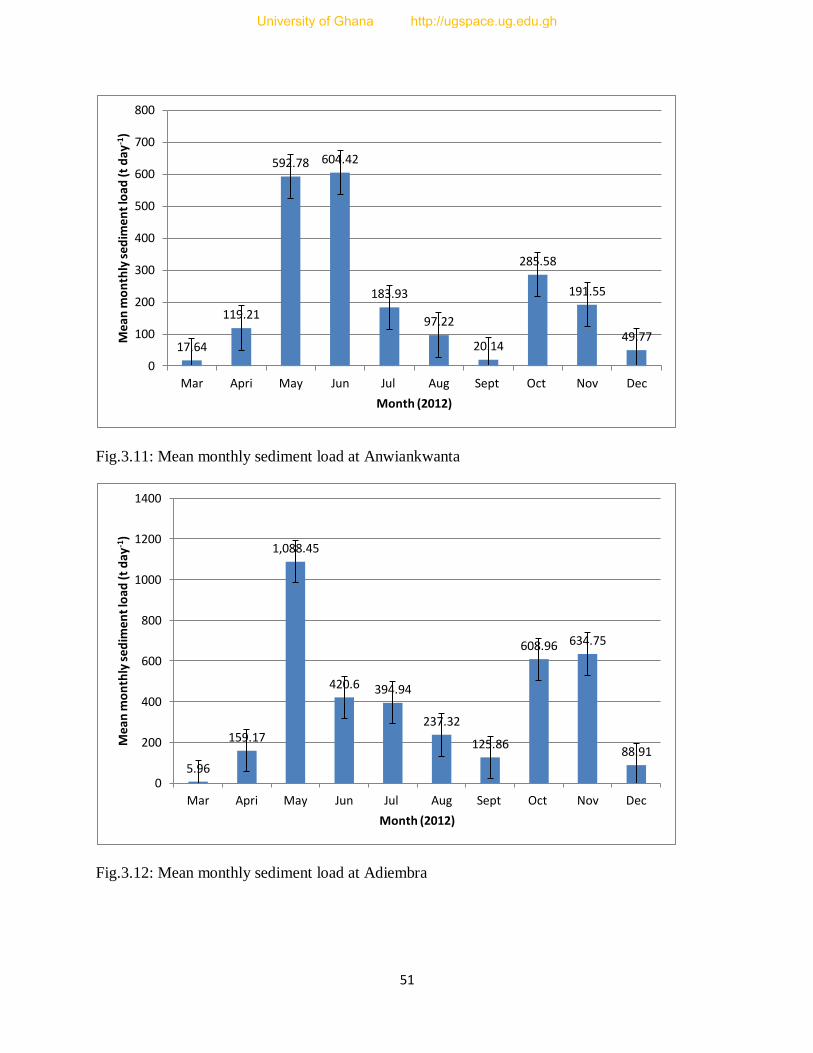
51

Fig.3.11: Mean monthly sediment load at Anwiankwanta

Fig.3.12: Mean monthly sediment load at Adiembra

17.64

119.21

592.78 604.42

183.93

97.22

20.14

285.58

191.55

49.77

0

100

200

300

400

500

600

700

800


Me

an m

on

thly

se

dim

en

t lo

ad (

t d

ay-1

)

Month (2012)

5.96

159.17

1,088.45

420.6 394.94

237.32

125.86

608.96 634.75

88.91

0

200

400

600

800

1000

1200

1400


Mea

n m

on

thly

sed

imen

t lo

ad (

t d

ay-1

)

Month (2012)


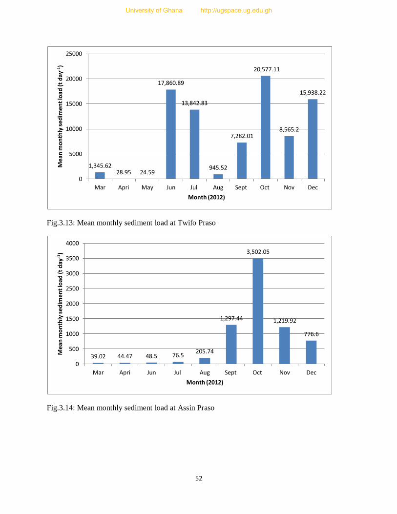
52

Fig.3.13: Mean monthly sediment load at Twifo Praso

Fig.3.14: Mean monthly sediment load at Assin Praso

1,345.62 28.95 24.59

17,860.89

13,842.83

945.52

7,282.01

20,577.11

8,565.2

15,938.22

0

5000

10000

15000

20000

25000


Me

an m

on

thly

se

dim

en

t lo

ad (

t d

ay-1

)

Month (2012)

39.02 44.47 48.5 76.5 205.74

1,297.44

3,502.05

1,219.92

776.6

0

500

1000

1500

2000

2500

3000

3500

4000

Mar Apri Jun Jul Aug Sept Oct Nov Dec

Mea

n m

on

thly

sed

imen

t lo

ad (

t d

ay-1

)

Month (2012)


53

Fig.3.15: Mean monthly sediment load at Sekyere Heman

specific suspended sediment yield for the whole Pra Basin at Sekyere Heman station was

329 t km-2

yr-1

(Table 3.2). At Adiembra for the Ofin Basin the specific suspended sediment yield

was slightly above 37 t km-2

year-1

, nearly 94 t km-2

yr-1

for the Birim at Akim-Oda, about 51 km-

2 year

-1 for the Oda at Anwiankwanta, and above 69 km

-2 yr

-1 at Brenase. The specific suspended

sediment yield of the drainage basin at Sekeyere Heman and that of the Birim Basin are higher

compared to those of other major drainage basins in Ghana and other tropical rivers. The yields

in these basins are higher than those obtained for the Black Volta (28 t km-2

yr-1

), White Volta

(33 t km-2

yr-1

), and Oti (63 t km-2

yr-1

) in Ghana (Akrasi, 2005). They are also higher than the

suspended sediment yields for other major rivers in Africa and South America including the

Niger (about 5 t km-2

yr-1

), Congo (16 t km-2

yr-1

), Nile (37 t km-2

yr-1

), and the Amazon (63 t

km-2

yr-1

). These values are; however, lower than that of the Ganges whose specific suspended

sediment yield is above 1,350 t km-2

yr-1

(Akrasi, 2005).

11,942.8 14,947.4

18,039

42,437.5

36,539.8

25,256.3

29,855.9

23,632.4

42,367.3

0

5000

10000

15000

20000

25000

30000

35000

40000

45000

50000

Mar Apri May Jun Jul Sept Oct Nov Dec

Me

an m

on

thly

se

dim

en

t lo

ad (

t d

ay-1

)

Month (2012)


54

Model results of a hypothesis test indicate a significant variation in sediment yield within

drainage basins with a p-value of 0.01 and an R2 to be 0.70 (Model1; Appendix A). Spearman

and Kendall correlation analyses showed very strong positive correlations between sediment

yield and drainage basin area with r values of 0.93 and 0.81 (Models2 & 3, Appendix A). These

models results are; however, in contrast with the inverse relationship model between sediment

delivery ratio and basin area. The inverse relationship has been explained in terms of decreasing

slope and channel gradients with increasing basin size and this increases opportunities for either

a temporary/permanent deposition to be associated in river channels, floodplains, valleys or the

base of slopes. Literature shows that mostly between 10-30% of gross erosion is transported into

river channels and this is what ends up at basin outlets (Golubev, 1982; Hadley and Shown,

1976; Walling, 1983). For instance, there is a 17% loss in sediment load along the Nile River

from Sudan to Egypt and along the Nazus River in Mexico, the conveyance loss in total

suspended sediment load is 25% (Walling, 1983).

The increasing levels of suspended sediment concentration and sediment yields downstream

are explained by the increasing human activities along and within the rivers particularly illegal

small scale mining. These illegal small scale mining activities become very intensive towards the

mouth of the Pra at Sekyere Heman because of increased volume of the river. At the upper

sections of the rivers such as Kibi (refer to Plate.1a in chapter one), Anyinam, Brenase, Konongo

etc the illegal mining is basically restricted to land fringing the banks due to the small river

channel but towards the middle sections such as Akim Oda, Assin Praso, Dunkwa-on-Ofin,

Twifo Praso and the mouth, the illegal mining activities take two forms; alluvial mining within

the river bed and channel bank mining (bank full stage) because the river channel is now wider

and deeper which enables the miners to ply within the channel (see Plate.1b in chapter one).


55

There is virtually no community without these miners, particularly from the middle section to the

mouth. On the Pra River they are found in every community from Sekyere Heman to Brenase, on

the Birim River from Assin Praso to Kibi, on the Ofin River from Foso downstream of

Adwumain to Adiembra and on the Oda River they are found from Bepotenten to

Anwiankwanta. These activities are primarily responsible for the entrainment of large quantities

of sediments into the rivers even at low flows from both bank mining activities and the discharge

of mine wastes into the rivers. Thick plumes of sediments are observed in transport in these mine

sites and the intensity of their activities does not promote much deposition of fluvial sediments.

For instance at Sekyere Heman and Twifo Praso, the illegal mining activities were just about 200

m upstream of the sampling stations and this is the major explanation to the exceptionally high

sediment levels in these stations. Interaction with locals in these communities indicated that, this

level of pollution of the rivers has been as a result of the illegal mining activities. Hitherto, the

water was very clean, clear of sediments and they used to depend on it for domestic chores, but

now that is impossible because the water looks very dirty and they cannot drink it any more.

The implication of the level of sediment load and transport patterns in the entire Pra Basin is

that, it poses a great threat to the sustainability of dams/reservoirs on these rivers and water

quality of the rivers in general as was discussed in the problem statement in chapter one.

According to managers of Ghana Water Company Limited in the Pra Basin particularly at Kibi,

Twifo Praso, Dunkwa-on-Ofin, Beposo and Sekyere Heman, the level of sediment and chemical

pollution of the water by these galamsey activities is increasing their cost of operation as more

chemicals have to be used in treating the water before it is supplied to consumers. The situation

is also causing the frequent break down of their equipment and this have therefore raised serious

concerns about these illegal mining activities as these illicit activities are threatening the water


56

treatment plants. Due to the deteriorated state of the water, most communities that do not have

access to potable water along the rivers now have to depend on boreholes for their domestic

water needs. Residents along the rivers complained of reduced stock of fish and crabs in the

rivers owing to the pollution resulting from the illegal mining. Also owing to the turbid state of

the water, residents are scared of swimming or bathing in the rivers for fear of contracting

diseases. These illegal mining activities have also been a great concern to Water Resources

Fig.3.16: Annual sediment yield.

Table 3.2: Annual suspended sediment load and specific suspended sediment yield for the

monitored stations in the Pra River Basin

River and station Drainage

Area

(km2)

Annual suspended

sediment yield

(t y-1

)

Annual specific

sediment yield

(t km-2

year-1

)

Oda at Anwiankwanta 1,288 66,094.1 51.3

Ofin at Adiembra 3,101 115,372.1 37.2

Birim at Akim Oda 3,104 290,775.6 93.7

Pra at Brenase 2,168 150,455.4 69.4

Pra at Assin Praso 9,235 220,907.1 23.9

Pra at Twifo Praso 2,0625 2,645,002.1 128.2

Pra at Sekyere Heman 22,758 7,489,290.1 329.1

NB: Drainage areas composed of upstream of stations draining into the station and these were

extracted in ArcGIS.

66,094 115,372 290,776 150,455 220,907

2,645,002

7,489,290

0

1,000,000

2,000,000

3,000,000

4,000,000

5,000,000

6,000,000

7,000,000

8,000,000

An

nu

al s

edim

ent

yiel

d (

t yr

-1)

Sampling stations


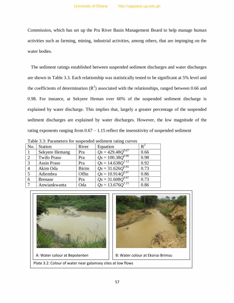
57

Commission, which has set up the Pra River Basin Management Board to help manage human

activities such as farming, mining, industrial activities, among others, that are impinging on the

water bodies.

The sediment ratings established between suspended sediment discharges and water discharges

are shown in Table 3.3. Each relationship was statistically tested to be significant at 5% level and

the coefficients of determination (R2) associated with the relationships, ranged between 0.66 and

0.98. For instance, at Sekyere Heman over 60% of the suspended sediment discharge is

explained by water discharge. This implies that, largely a greater percentage of the suspended

sediment discharges are explained by water discharges. However, the low magnitude of the

rating exponents ranging from 0.67 – 1.15 reflect the insensitivity of suspended sediment

Table 3.3: Parameters for suspended sediment rating curves

No. Station River Equation R2

1 Sekyere Hemang Pra Qs = 429.48Q0.67

0.66

2 Twifo Praso Pra Qs = 100.38Q0.90

0.98

3 Assin Praso Pra Qs = 14.638Q1.12

0.92

4 Akim Oda Birim Qs = 31.626Q0.95

0.73

5 Adiembra Offin Qs = 10.914Q0.97

0.86

6 Brenase Pra Qs = 31.608Q0.97

0.73

7 Anwiankwanta Oda Qs = 13.676Q1.15

0.86

Plate 3.2: Colour of water near galamsey sites at low flows

B: Water colour at Ekorso Brimsu

A: Water colour at Bepotenten


58

concentration to increases in discharges, which implies the rivers remain turbid over a wide

range of flows, and the suspended sediment concentrations remain relatively high even during

low flows. The insensitive nature of sediment discharge to water discharge could be attributed to

the alluvial illegal gold mining activities practiced within the river channel and the basin

resulting in the remobilzation of deposited channel sediments. This results in constant discharge

of sediments into the fluvial sediment transport. See how turbid the rivers are at two galamsey

sites; Bepotenten and Ekorso Brimsu on the Oda and Birimsu Rivers respectively at low flows

(Plate 3.2).

Since the curves were derived from one year flows, they are likely to be associated with errors.

The use of only one year of data means the curves may not provide accurate estimates of long

term mean sediment discharges of the basins. Sediment concentrations were determined using

both the integrated and dip samplings with the dip samples being corrected by a correction factor

of the integrated samples. This will definitely introduce some errors. Also sampling was also not

according to the hydrological regime/seasonality of flow but calendar based; hence certain

critical flows were missed irrespective of the number of samples taken particularly in stations

where people could not be engaged to undertake dip sampling. For lack of previous flows and

concentration data, the accuracy of these curves could not be evaluated but could be associated

with error margins due to the reasons outlined above. According to Horowitz (2003) and Walling

(1977a; 1977b), the sediment rating-curve method tends to under predict high, and over predict

low suspended sediment concentrations when flow is not constant throughout the day. As such,

the range of errors associated with concomitant flux estimates for relatively short time-frames

(e.g. daily, weekly) are likely to be substantially larger (<±20%) than those associated with

longer time-frames (e.g. quarterly, annually) because the over and under predictions do not have


59

sufficient time to balance each other. The evaluations indicate that over periods of 20 or more

years, errors of <1% can be achieved using a single sediment rating curve based on data

spanning the entire period. In either case, hydrologically based sampling, as opposed to calendar-

based sampling is likely to limit the magnitude of flux estimation errors.

3.3 Conclusion

The annual specific sediment yield measurements in the Pra Basin are higher than most tropical

rivers including those in Ghana. Illegal alluvial gold mining within the rivers and the basin is one

of the likely underlying forces injecting sediments into the rivers as compared to other forces.

This large sedimentation levels have socio-economic and environmental implications as this is

increasing the cost of potable water supply, and break down of water equipment. Also residents

are denied of their cheap sources of protein needs as a result of the reduced stock of fish and

crabs in the water bodies.


60

Chapter Four

Sediment Source Analysis

4.0 Introduction

There is an increasing need to determine sources of sediments in fluvial sediment

transport owing to their environmental impacts. For instance, in Africa, the on-site

problems caused by enhanced soil erosion include a reduction of soil depth and organic

matter content (El Wakeel & Astatke, 1996; Lal, 1996a), the depletion of plant-available

nutrients (Ghuman & Lal, 1991; Lal, 1996b) and a reduction of water storage capacity in

the root zone (El-Swaify, 1993). These can all reduce crop yields (Lal, 1993) and are

compounded by the inability of the typical subsistence farmer to provide the inputs

necessary to restore soil quality (El-Swaify, 1993).

In response to these sediment-related environmental problems, major soil conservation

programmes have been established in several African countries, including Kenya

(Wenner, 1980), Zimbabwe (Elwell, 1978) and Zambia (Bezuneh et al., 1995). Such

schemes have, however, been hampered by a multitude of physical, socioeconomic,

demographic and political constraints, and by limited resources (Collins et al., 2001).

Information on sediment sources is required to design effective sediment and non-point

pollution control strategies. This will provide an improved understanding of erosion and

suspended sediment transport within a basin which is an essential precursor to

establishing sediment budgets, developing distributed sediment yield models, and

interpreting sediment yields in terms of landscape evolution (Walling et al., 1993). As

observed in the previous chapter, sediment yield levels in the Pra Basin are high and this

calls for public concern due to the environmental and health related impacts.Traditional

methods of watershed monitoring for suspended sediments are inadequate to provide


61

information on fluvial processes taking place within a watershed (Mukundan et al.,

2009). The fingerprinting approach has proved to be an effective way for tracking

sediment movement within a watershed in terms of both source type and spatial origin

(Walling, 2005). Consequently, the fingerprinting technique was adopted to identify

sediment sources and quantify the various pathways of sediment origin within the Pra

Basin. The chapter presents research materials and methods employed in carrying out this

tracer study and findings of the study.


Sediment source tracking was performed on the basis of sub-basins using the finger print

method (Gruszowski et al., 2003). The following potential sediment source types were

sampled for analysis; for surface erosion (arable top soils, illegal mining sites,

path/untarred roads leading to rivers, gullies and gutters from settlements and farms into

streams) and for bank erosion (channel banks). Sampling sites of these potential sediment

sources were determined through field investigations and interviews with the local

communities to identify areas of active sediment erosion (Davis and Fox, 2009).

To accommodate local spatial variability in 210

Pb in the surface soil, core samples of

depth 10 cm within plot sizes of 15×15 m2 at grid intervals of 3× 3 m were taken at each

site with an improvised 5 cm pvc pipe as a corer. Samples were composited for analysis

(Nagle et al., 2007; Walling, 2004). Bank sediments were collected by scrapping channel

wall sediments (Davis and Fox, 2009). Suspended sediments were sampled at the

catchment outlets of sub-basins using the depth integrated sampler based on the equal-

width-incremental approach across a channel transect (Davis and Fox, 2009; Edwards

and Glysson, 1999; Matisoff and Whiting, 2011) and composited for analysis to account

for the spatial variability in 210

Pb concentration across the section. Collected surface


62

sediments were placed in polyethene bags whiles those of suspended sediments were in

plastic bottles which were preserved in iced chests (Ohio EPA, 2001) to minimize

biological and chemical changes from the time of collection to the time of analysis.

Samples were collected in September when flows were high because 210

Pb environmental

radionuclides are known to fallout highest with increasing precipitation (Matisoff and

Whiting, 2011).

All source material samples were air-dried, ground in a mortar and dry-sieved to 63µm

because radionuclides tend to have higher sorption to finer soils (Matisoff and Whiting,

2011) and also to facilitate direct comparison of suspended sediment and source samples

(Collins et al., 2001). Suspended sediments were centrifuged and the supernatant

discarded, recovered solids were oven dried. Samples were then analyzed for 210

Pb using

Atomic Absorption Spectrophotometer (AAS). The AAS digestion procedure for lead

210 was as follows:

0.5g of sample was measured into labelled 100 ml polytetraflouroethylene PTEF Teflon

bombs. 6ml of Concentrated HNO3 and 5ml of concentrated HCL 38% were added in a

fume chamber. Samples were then loaded on a microwave carousel. The vessel cap was

secured tightly using an appropriate screw tool. The complete assembly was microwave

irradiated for 21min in a Milestone microwave Labstation (Ethos 900) using the

following operation parameters; 250w for 5 min, 0w for 1 min, 250 w for 10 min, 450w

for 5 min, and 5 min allowed for venting (Milestone Cook Book, 1996). After digestion

the Teflon bombs mounted on the microwave carousel were cooled in a water bath to

reduce internal pressure and to allow volatilized material to re-solubilize. The digest was

made up to 20 ml with ddH20 and assayed for the presence of metals on a Varian

AA240FS Atomic Absorption Spectrophotometer in an acetylene –air flame. Typical

count times on gamma detectors were in the order of ~84 k s-1

(Wallbrink et al. 2003).


63

To quantify the relative contributions of bank and surface sources, values of 210

Pb

concentration were analysed using a simple mixing model which has been used

effectively by Mukunda et al., (2009), Nagle and Ritchie, 2004 and Nagle et al., (2007);

Cs =

…………….. (4.1),

where Cs (%) is the percentage contribution from surface sources; Pr is the value of 210

Pb

for stream sediments, Ps the concentration value of 210

Pb in surface sediment sources and

Pb the value of 210

Pb for bank materials.


Tables 4.1 - 4.4 illustrate the mean concentration of 210

Pb for each of the surface sample

types as well as the average concentration of all the surface samples captioned mean

surface soil. The mean concentration levels of bank sediments and stream sediments are

also provided for each sub-catchment. Results of individual surface and bank samples are

illustrated in Appendix B. Mean concentration levels of 210

Pb for bank sediments were

generally lower than most surface samples (Table 4.1 – 4.4) except at Oda Basin. The

lowest mean concentration of 210

Pb for bank materials was 0.89 Bq/kg and was recorded

in the Birim Basin and the highest value of 3.09 Bq/kg occurred in the Pra Sub-basin

(Tables 4.3 and 4.4). However the lowest mean surface soil value was recorded in Birim

Basin (1.34 Bq/kg) whiles the highest was in the Pra Sub-basin (3.40 Bq/kg) (Tables 4.2

and 4.3).

Roads that are not tarred and settlements (urban landscapes) were found to have the

highest mean value of 210

Pb in surface samples as compared to other surface samples.

The rationale for this high concentration of 210

Pb in these samples is due to the well

exposed and less disturbed state of these landscapes as compared to soils of farms,


64

Table 4.1: Mean 210

Pb Concentration levels for stream sediment and potential source materials in Birim Sub-basin

Tracer Galamsey

(n = 7)

Road &

Bridge(n = 7)

Farm

(n = 8)

Settlement

(n = 8)

Gully

(n = 3)

Gutter

(n = 2)

Mean surface

soil (n = 47)

Bank Sediment

(n = 12)

Stream

Sediment 210

Pb Bq/kg 1.45 1.79 1.43 1.65 1.06 0.74 1.34 0.89 1.10

Table 4.2: Mean 210

Pb Concentration levels for stream sediment and potential source materials in the Pra main basin

Tracer Galamsey

(n = 9)

Road & Bridge

(n = 21)

Farm

(n = 7)

Settlement

(n = 9)

Gully

(n = 1)

Gutter

(n = 10)

Mean surface

soil (n = 72)

Bank Sediment

(n = 15)

Stream

Sediment 210

Pb Bq/kg 2.32 4.02 2.88 3.31 0.68 4.25 3.40 3.09 3.18

Table 4.3: Mean 210

Pb Concentration levels for stream sediment and potential source materials in Oda Sub-basin

Tracer Galamsey

(n = 5)

Road & Bridge

(n = 2)

Settlement

(n = 4)

Gully

(n = 2)

Gutter

(n= 4)

Mean surface

soil (n=29)

Bank Sediment

(n=12)

Stream

Sediment

210Pb Bq/kg 0.44 0.55 1.01 2.34 2.96 1.77 2.12 2.24

Table 4.4: Mean 210

Pb Concentration levels for stream sediment and potential source materials in Ofin Sub-basin

Tracer Galamsey

(n = 2)

Road & Bridge

(n = 8)

Farm

(n = 2)

Settlement

(n= 2)

Gully

(n= 2)

Gutter

(n= 3)

Mean surface

soil (n=27)

Bank Sediment

(n = 8)

Stream

Sediment 210

Pb

Bq/kg

2.25 2.22 1.13 2.84 0.85 0.52 1.54 1.01 1.16

Table 4.5: Contribution of bank material and surface soil sources to suspended sediment load in the various sub-catchments

River

Basin

Birim Pra Oda Ofin

Source

Type

Surface

soil

Bank

sediment

Surface

soil

Bank

sediment

Surface

soil

Bank

sediment

Surface

soil

Bank

sediment 210

Pb

(%)

47 53 29 71 34 66 28 72


65

galamsey, and gullies which are frequently being mixed/tilled or eroded. The exposed

urban soils promote the accumulation of 210

Pb radio-nuclide fallouts. Samples from

gutters were also high in 210

Pb concentration levels with a minimum value of 0.52 Bq/kg

in the Offin Basin and a maximum of 4.25 Bq/kg in the main Pra Sub-basin (Table 4.2

and 4.4). Generally lower levels of 210

Pb in surface samples were found in sites of active

erosion. In all the basins, 210

Pb mean levels in bank sediments were found to be lower

than mean 210

Pb samples of most surface sites. For instance except gutter samples in the

Birim Basin and then gully and gutter samples in the Ofin Basin, all other surface

samples had a higher 210

Pb levels than bank materials (Tables 4.1 and 4.4). However, in

the Pra and Oda Basins, bank sediments were relatively high in 210

Pb concentration than

most surface materials (Tables 4.2 and 4.3).

Lower levels of bank sediment samples and surface samples were recorded in localities

of very active bank erosion and surface erosion (Tables 4.6; 4.8 and 4.9; Appendix B).

Areas of active bank erosion do not promote the accumulation of 210

Pb fallouts in the

soils of river banks as they are constantly being washed away into the river. Nagle et al.,

2007 also attributed low levels of an environmental radionuclide 137

Cs in bank sediments

to active bank erosion. Also recent illegal mines sites (galamsey) also recorded lower

values of 210

Pb (Tables 4.6 – 4.9; Appendix B). For instance at Kibi, an abandoned

illegal mined site had 3 Bq/kg 210

Pb concentration as compared to an adjacent site with a

value of 1.2 Bq/kg where mining was ongoing (Table 4.6; Appendix B). Soils are dug

from pits of 20 m or more by the miners where 210

Pb fallouts do not reach, because

maximum concentrations of 210

Pb in soils are usually found at the surface decreasing

exponentially with depth, and reaching undetectable levels at depths greater than 10 cm.

The mixing of top soils rich in 210

Pb with underground mined soils or the burial of top

soils due to the mining activities account for the low lead 210 values. Thus samples of


66

adjacent soils had higher values than those of galamsey site. These observations are in

line with literature. According to Walling et al., (1993), in undisturbed soils, 210

Pb are

concentrated in the upper 10 cm of the soil profile, whereas in cultivated soils this

radionuclide will be mixed throughout the plough layer and surface concentrations will

be much lower. Also subsoil horizons below 25 cm and exposed river banks (apart from

the upper 10 cm) will contain zero or only very low levels of unsupported 210

Pb. Also

lower levels of 137

Cs in certain plots relative to others was explained by soil mixing due

to cultivation (Nagle and Ritchie, 1999).

The simple sediment mixing model results derived using equation (4.1) show that a

higher percentage contribution of sediments into the fluvial sediment transport is coming

from bank sediments with a range of 53 – 72% (Table 4.5). The lowest estimated bank

sediments contribution is in the Birim Basin (53%) whiles the highest is recorded in the

Ofin Basin (72%). Conversely, the lowest surface soil sediment source (28%) is in the

Ofin Basin whiles the highest surface sediment source is in the Birim Basin (47%) (Table

4.5). The model results are buttressed by the hypothesis test that stream bank erosion is a

significant source of sediment transport in the main Pra Basin and its sub-catchments

with a p-value of 0.0003 and an R2-value of 0.99 (Appendix B). The p-value of surface

soil is; however, 0.08 with a higher AIC value of -4.9 as compared to -27.3 for bank

sediments (Appendix B).

Due to the good vegetative cover (details in chapter 6), soils are well protected and

coupled with low gradient of the catchment which is less than 20 degrees, surface erosion

is very low. Collins et al., (2001) also made a similar observation that, due to the

increased cover density provided by natural vegetation soil erosion from surface soils

declined from the dry to wet season. On the other hand, channel erosion at the middle

section and activities of alluvial small scale mining activities within the rivers entrain


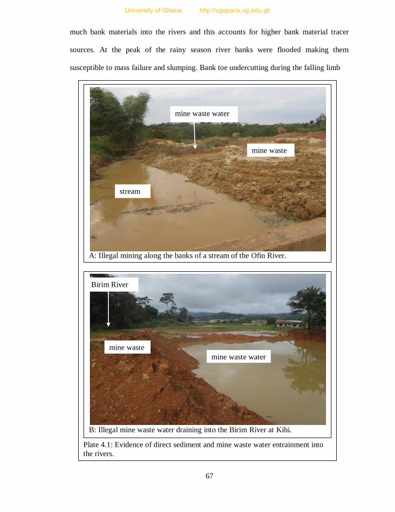
67

much bank materials into the rivers and this accounts for higher bank material tracer

sources. At the peak of the rainy season river banks were flooded making them

susceptible to mass failure and slumping. Bank toe undercutting during the falling limb

Plate 4.1: Evidence of direct sediment and mine waste water entrainment into

the rivers.

A: Illegal mining along the banks of a stream of the Ofin River.

B: Illegal mine waste water draining into the Birim River at Kibi.

stream

mine waste water

Birim River

mine waste

mine waste

mine waste water


68

stage of flow hydrograph resulted in the removal of bank material and bank collapse into

the river channel. Bank erosion was observed to be very severe in the middle course of

the tributaries.

This result is in common with findings of chapter three and chapter five. It was observed

in the previous chapter that in the upper sections of the river where there are no activities

of illegal mining, river water was of low turbidity and of low suspended sediment

concentration. However at the middle and lower sections where small scale alluvial gold

mining is intense, the colour of the rivers tended to be gray or brown and are

characterised by very high suspended sediment levels. The underlying reason accounting

for the high sediment injection into the rivers as discussed earlier is because, most of the

miners undertake alluvial mining within the river bed and channel banks and this entrains

sediments directly into the river or it results in the remobilization of deposited sediments

into the sediment transport system.

Besides this practice, other miners who are along the river/stream banks, discharge both

their mine waste sediments or water into nearby streams and rivers to avoid the flooding

of their sites (Plate 4.1). These mine waste water are very turbid and thus generate

plumes of sediments in the rivers which discolours the water. And there are hundreds of

these miners strung along all the major tributaries and most streams within the basin.

Also due to the exposed nature of these galamsey landscapes (Plate 1), rain drops

dislodge soil particles (rain splash) causing sheet erosion. Hence run-off/overland flow

drains directly as flash floods into the streams and rivers increasing the sediment

concentration levels. Similarly, it has been observed that significant soil erosion by

rainsplash, sheetwash and rilling is prominent in exposed areas of bare soils (Collins et

al., 1997; Collins et al., 2001). Such erosion is accentuated by high rainfall erosivities

during frequent thunderstorms which are characteristic of the tropics (Stocking & Elwell,


69

1976; Obi & Salako, 1995). In fact, the nature of the sediment entrainment from these

mine sites can not in any way be compared to bank erosion by hydraulic processes.

4.3 Conclusion

In this chapter a tracer technique using 210

Pb environmental radionuclide has been

employed to determine that much suspended fluvial sediments in transport are originating

from bank materials. The method used in this study did not allow the discrimination

between the contributions of the various subsurface sources to the fluvial sediment in

transport. A combination of human activities (galamsey) and bank erosion are however,

the plausible explanatory factors accounting for the entrainment of bank sediment into the

sediment transport budget. Though the study could not differentiate between fingerprints

of galamsey materials from those of bank erosion, however the relatively high levels and

trends in suspended sediment discharge throughout the season even at low flows as

shown in the previous chapter attest to the fact that, illegal mining could be the major

source of bank sediments discharge into the rivers. Additional information is provided in

the next chapter on the state of bank erosion of channel walls within the river valleys.


70

Chapter Five

Changes in River Channel

5.0 Introduction

Changes in river channels as a result of bank erosion and deposition cause significant

damage to infrastructure (e.g., bridge crossings, pipes), losses of fertile agricultural soil,

and a degradation of stream water quality (Bertrand, 2010) because erosion and

deposition highly impact the amount of sediment transported to a stream (Hayes, 2004).

Bank erosion plays a very important role in river channel dynamics, meander

development, and catchment sediment systems (Church and Slaymaker, 1989). Channels

are widened; meander loops are severed to form ox-bow lakes and large volumes of

sediments can be entrained into channels due to bank erosion and bank failure of river

valleys. River banks have been shown to act as key sediment sources and sinks; in many

different types and sizes of drainage basins, and can supply over 50% of catchment

sediment output (Church and Slaymaker, 1989; Lawler et al., 1999).

As demonstrated in chapter four, bank materials are the main source of suspended

fluvial sediments in the Pra Basin. Bank erosion; therefore, constitutes an intricate

physical, socio-economical, and ecological problem requiring an improved understanding

of the key processes governing bank erosion (Bertrand, 2010). Knowledge of the rates,

patterns and dynamics of bank erosion events that release sediment and any associated

contaminants to the fluvial system is fundamental, therefore, to a complete understanding

of the fluvial sediment transport regime, including fluxes to estuarine zones (Lawler et

al., 1999) and channel stability. In this chapter, an attempt is made to quantify the rates

and spatial variability in bank erosion and channel stability in order to evaluate the

relative importance of bank sediment supplies to the sediment budget in transport in the


71

Pra Basin and its sub-catchments by undertaking bank erosion measurements at selected

cross sections. The underlying fluvial and sub-aerial processes influencing the dynamics

in channel stability were also investigated.


Bank erosion was assessed using erosion pin approach (e.g. Bertrand, 2010; Billi, 2008;

Lawler et al., 1997; Schoonover et al., 2007). Galvanized steel rods of 6 mm thick and 45

cm long were inserted into channel walls and their levels of exposure measured with a

ruler (Plate.5.1). Depending on the depth of the bank face, pins were inserted at each

bank face at 1 × 1 m or 0.5 × 0.5 m horizontal and vertical grid intervals. Pins were

pressed into the soil or lightly tapped with a hammer until 5 cm of the pin remained

exposed.

Plate.5.1: Erosion Pin at the bank of the Birim River at Akim Oda


72

Pins were identified at cross sections with bench marks and numbered sequentially in

downstream direction. The first pin in each cross section was placed on the bank toe

approximately 3 cm above base flow water surface elevation and the last pin was placed

below bankfull of the stream channel.

This elevation was chosen to allow pin measurement during normal flow conditions.

Pins were inserted in March when flows were low and monitored during low flows for

one year. The first measurement was taken in August/September of the same year at sites

where it was possible and in March the following year when flows were low. The level of

exposure of the rod is an indication of the extent of bank erosion. Pins were reset to the 5

cm after monitoring visits (e.g. Bartley et al., 2008; Lawler, 1993; Staley et al., 2006).

Soil surface disturbance was minimized as much as possible while placing pins and

when measurements were being taken. Reaches that were chosen for the bank erosion

measurements were based on reconnaissance survey to identify areas of active channel

erosion (Bertrand, 2010). Also, channel reaches undisturbed by human activities and

artificial structures; as much as possible, were chosen to avoid impact of human activities

on bank retreat (Lawler et al., 1997; Schoonover et al., 2007).

To estimate the amount of bank sediments into the river sediment transport, the mass of

sediments eroded into the river channel was estimated by determining the volume of

eroded sediments using equation (5-1), multiplying this volume by soil density (ρ), ρ

density of wet soil (1920 kg/m3) (Freeze and Cherry, 1979):

Volume = length × height × width .......................................(5-1),

. To determine the susceptibility of bank sediments to erosion, bank sediment samples

were collected at each site and analysed to determine the median grain size (D50) and the

percent clay and silt (Bartley et al. 2008) of bank sediments.


73


Tables 5.1 – 5.6 show the annual rate of bank erosion and deposition analyses from

erosion pin measurements. Significant channel erosion was recorded at Akim Oda (Birim

River), Ejesu (Oda River) and Adiembra (Ofin River) whiles at Anyinam (Birim River),

Amuanda Praso and Brenase both on the Pra River, bank erosion was low.

River channel at Anyinam was characterized by very low bank erosion and deposition,

even two erosion pins never receded and the maximum annual mean erosion recorded

was about 4 cm whiles deposition was very intense, with alluvial deposits of between 2 –

65 cm (Table 5.1). Akim Oda; however, experienced very active bank erosion

characterized by bank failure (Tables 5.3). Here all erosion pins receded with the lowest

eroded pins recession being nearly 4 cm and the highest about 20 cm of exposure. On the

Birim River, mean annual bank erosion increased downstream from 1.3 cm at Anyinam

to 9.9 cm at Akim Oda (Tables 5.1 and 5.3).

The increase in bank erosion downstream is attributed to an increase in flow/discharge

downstream resulting in bank wearing and weakening, bank collapse by flood waters,

especially at bankfull stage. This observation is in line with findings of Lawler et al

(1997, 1999) who observed that, from mid-basin downstream the optimum combination

of water surface slope, channel cross- section geometry and discharge is obtained, hence

available stream energy is likely to peak resulting in the dominance of stream

entrainment processes such as bank wearing and mass failure of channel banks. In the

upper reaches of river basins, stream power is low because of low discharges, despite

steep bed slopes, thus limiting the available energy for fluid entrainment of bank

materials and banks are also too small to be susceptible to mass failure (Lawler et al.,


74

1997; Lawler et al., 1999) (Plate.5.2). This promotes channel bed incision with low bank

erosion characterised by step-pools and bars in the dry season (Plate.5.2).

Monitored channel banks of the main Pra River were also characterized by both erosion

and deposition (Tables 5.2 and 5.4). At Amuanda Praso, the right bank was more erodible

than the left bank, whereas at Brenase it was the vice versa. Mean annual bank erosion at

Amuanda Praso (4 cm) was almost twice the bank wearing at Brenase (2.3 cm). Bank toe

erosion at both stations was greater than towards the bankfull stage. However, on the Pra

River, bank erosion decreased downstream by 1.6 cm between Amuanda Praso and

Brenase.

Just like Anyinam, the river channel at Ejesu on the Oda River was experiencing both

erosion and accretion with the mean annual bank erosion almost 11 cm (Table 5.5). The

lowest eroded pin was just above 2 cm and the highest eroded point was above 26 cm.

The opposite bank was; however, undergoing sediment deposition. Unlike the other river

channels, both banks of the Ofin River at Adiembra was subjected to bank erosion and

the annual mean erosion at both right and left banks was above 2 and 8 cm respectively.

In a nutshell, the retreat magnitudes observed in this study are lower than rates such as

8.3 – 44 cm obtained by Lawer et al., (1999) on Swale-Ouse system, northern England.

These values are also lower than the global average, and lower than expected for a

tropical river system, particularly when compared with other tropical rivers such as the

Luangwa River in Zambia, where erosion is as high as 33 m yr-1

(Bartley et al., 2008;

Gilvear et al., 2000).


75

Table 5.1: Annual bank erosion or deposition rates at Anyinam

Date 5th March 2013

Length of exposure/deposition of pins/cm (“+” erosion

and “-” deposition)

River Station Bank Bank Location Pin 1 Pin 2 Pin 3 Pin 4 Pin 5

Birim Anyinam Left Top 0.0 0.0 0.5 3 1

Left Bottom 1.0 0.5 2.0 1.5 3.7

Right Top Deposition of sediments of depth between 2 – 17cm

Right Bottom Deposition of sediments of depth between 20 – 65cm

Average annual bank erosion (cm) 1.3

Volume of eroded sediments (cm3) 33,800

Mass of eroded bank sediments (tonnes/yr) 64,896

Gridded interval: Horizontal (1 m), Vertical (0.65 m)

Table 5.2: Annual bank erosion or deposition rates at Amuanda Praso

Date 5th March 2013

Length of exposure/deposition of pins/cm

(“+” erosion and “-” deposition)

River Station Bank Bank Location Pin 1 Pin 2 Pin 3

Pra Amuanda Praso Right Top 5.8 1.5 3

Right Middle 3 1 5

Right Bottom 5.5 4 6.4

Left Top buried buried buried

Left Middle buried buried 2.5

Left Bottom 6 6 5.5

Average annual right bank erosion (cm) 3.9



Gridded interval: 1 m by 1 m


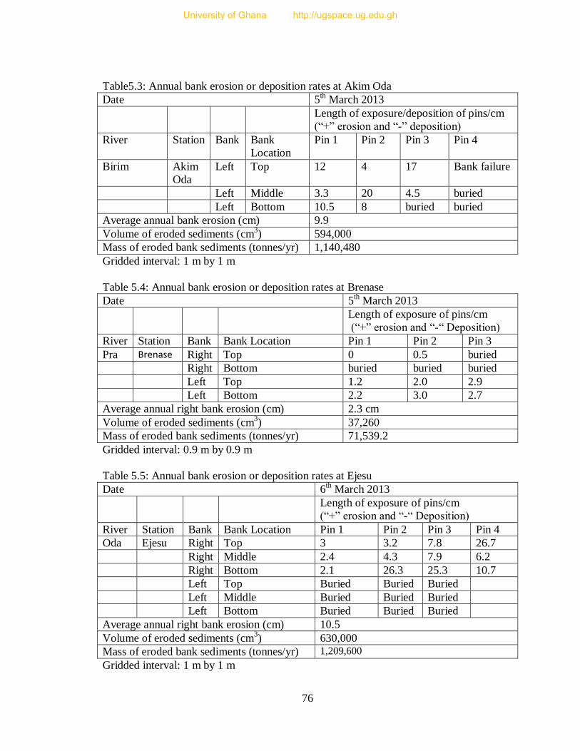
76

Table5.3: Annual bank erosion or deposition rates at Akim Oda

Date 5th

March 2013

Length of exposure/deposition of pins/cm

(“+” erosion and “-” deposition)

River Station Bank Bank

Location

Pin 1 Pin 2 Pin 3 Pin 4

Birim Akim

Oda

Left Top 12 4 17 Bank failure

Left Middle 3.3 20 4.5 buried

Left Bottom 10.5 8 buried buried

Average annual bank erosion (cm) 9.9


Mass of eroded bank sediments (tonnes/yr) 1,140,480


Table 5.4: Annual bank erosion or deposition rates at Brenase

Date 5th March 2013

Length of exposure of pins/cm

(“+” erosion and “-“ Deposition)

River Station Bank Bank Location Pin 1 Pin 2 Pin 3

Pra Brenase Right Top 0 0.5 buried

Right Bottom buried buried buried

Left Top 1.2 2.0 2.9

Left Bottom 2.2 3.0 2.7

Average annual right bank erosion (cm) 2.3 cm


Mass of eroded bank sediments (tonnes/yr) 71,539.2

Gridded interval: 0.9 m by 0.9 m

Table 5.5: Annual bank erosion or deposition rates at Ejesu

Date 6th March 2013



River Station Bank Bank Location Pin 1 Pin 2 Pin 3 Pin 4

Oda Ejesu Right Top 3 3.2 7.8 26.7

Right Middle 2.4 4.3 7.9 6.2

Right Bottom 2.1 26.3 25.3 10.7

Left Top Buried Buried Buried

Left Middle Buried Buried Buried

Left Bottom Buried Buried Buried



Mass of eroded bank sediments (tonnes/yr) 1,209,600



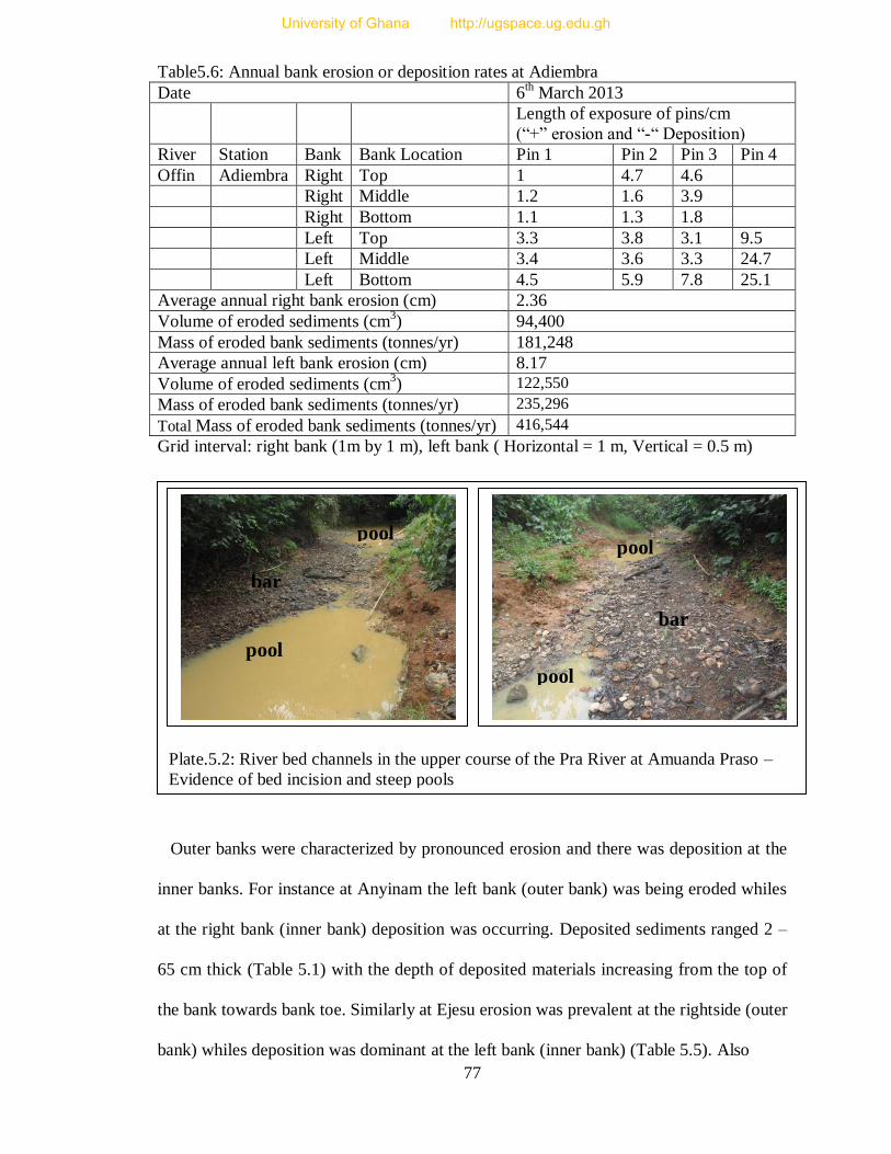
77

Plate.5.2: River bed channels in the upper course of the Pra River at Amuanda Praso –

Evidence of bed incision and steep pools

Table5.6: Annual bank erosion or deposition rates at Adiembra

Date 6th March 2013



River Station Bank Bank Location Pin 1 Pin 2 Pin 3 Pin 4

Offin Adiembra Right Top 1 4.7 4.6

Right Middle 1.2 1.6 3.9

Right Bottom 1.1 1.3 1.8

Left Top 3.3 3.8 3.1 9.5

Left Middle 3.4 3.6 3.3 24.7

Left Bottom 4.5 5.9 7.8 25.1




Average annual left bank erosion (cm) 8.17



Total Mass of eroded bank sediments (tonnes/yr) 416,544

Grid interval: right bank (1m by 1 m), left bank ( Horizontal = 1 m, Vertical = 0.5 m)

Outer banks were characterized by pronounced erosion and there was deposition at the

inner banks. For instance at Anyinam the left bank (outer bank) was being eroded whiles

at the right bank (inner bank) deposition was occurring. Deposited sediments ranged 2 –

65 cm thick (Table 5.1) with the depth of deposited materials increasing from the top of

the bank towards bank toe. Similarly at Ejesu erosion was prevalent at the rightside (outer

bank) whiles deposition was dominant at the left bank (inner bank) (Table 5.5). Also

pool

bar

bar

pool

pool pool


78

bank incision increased towards bank toe due to increases in flow particularly at the

middle course where flows are generally at the mid-bank section throughout the year,

bank undercutting is very pronounced resulting in cantilever failures. For instance, at

Amuanda Praso, there is active bed incision as illustrated by the level of recession of the

bottom pins on both banks (Table 5.3 and Fig.5.3).

According to Bertrand (2010) and Lawler et al (1999) bank toe erosion is triggered due

to shear stress exerted by the flow, which can lead to bank undercutting near the toe or

mid-section region. This undercutting over-steepened the bank height making the bank

more susceptible to mass failure and slumping (Lawler et al., 1999). These findings are

similar to results of Lawler (1999), that bank retreat is the integrated product of three

interacting processes (i.e. weathering and weakening, fluvial erosion and mass-wasting),

with mass failures and fluvial erosion typically dominating in the middle to lower

portions of a drainage basin. This reinforces the point that fluvial erosion and mass

failures are both significant contributors to the total volume of fluvial sediment transport

as observed by Luppi et al (2009) along the Cecina River (Central Italy).

Steep banks were also subjected to cantilever bank failure due to undercutting and bank

toe erosion whiles on gentle slopes erosion is by soil creep and this results in sediment

deposition at the base of channels and burial of erosion pins. Active bank incision was

also very serious along outer banks of meander loops than straight channels. Buried pins

due to either bank failure or deposition could not be measured and insertion of new pins

was not possible in the unconsolidated sediments. There were also erosion measurement

sites close to the mouth of Ofin and Oda Rivers at Adeboa and Bepotenten which were

vandalised by galamsey activities and new pins could not be inserted. The vandalization

of sites by galamsey operators downstream of the Oda and Ofin Rivers at Bepotenten and

Adeboa respectively prevented the downstream variability trend assessment in bank


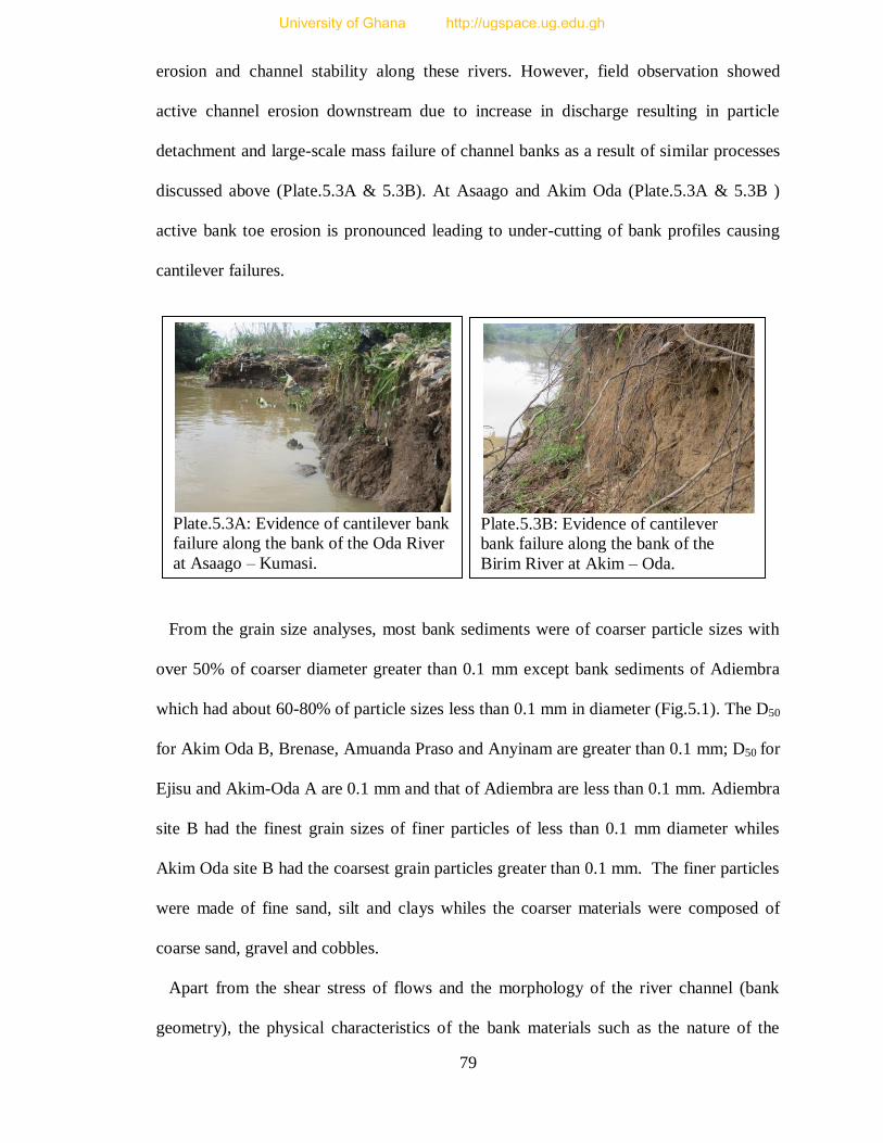
79

erosion and channel stability along these rivers. However, field observation showed

active channel erosion downstream due to increase in discharge resulting in particle

detachment and large-scale mass failure of channel banks as a result of similar processes

discussed above (Plate.5.3A & 5.3B). At Asaago and Akim Oda (Plate.5.3A & 5.3B )

active bank toe erosion is pronounced leading to under-cutting of bank profiles causing

cantilever failures.

From the grain size analyses, most bank sediments were of coarser particle sizes with

over 50% of coarser diameter greater than 0.1 mm except bank sediments of Adiembra

which had about 60-80% of particle sizes less than 0.1 mm in diameter (Fig.5.1). The D50

for Akim Oda B, Brenase, Amuanda Praso and Anyinam are greater than 0.1 mm; D50 for

Ejisu and Akim-Oda A are 0.1 mm and that of Adiembra are less than 0.1 mm. Adiembra

site B had the finest grain sizes of finer particles of less than 0.1 mm diameter whiles

Akim Oda site B had the coarsest grain particles greater than 0.1 mm. The finer particles

were made of fine sand, silt and clays whiles the coarser materials were composed of

coarse sand, gravel and cobbles.

Apart from the shear stress of flows and the morphology of the river channel (bank

geometry), the physical characteristics of the bank materials such as the nature of the

Plate.5.3A: Evidence of cantilever bank

failure along the bank of the Oda River

at Asaago – Kumasi.

Plate.5.3B: Evidence of cantilever

bank failure along the bank of the

Birim River at Akim – Oda.


80

bank materials (texture/particle sizes) and plant cover strongly influenced the degree of

bank erosion. High cohesive forces of finer particles particularly silt and clay made

certain banks a bit resistant to erosion as compared to the coarser zones. This is because

cohesive materials resist erosion by a complex set of characteristics related to the

existence of electro-chemical bonds between individual particles (Simon and Collison,

2001). For instance, at Akim Oda site B, due to the looseness of bank materials, bank toe

erosion and bank failure were very pronounced resulting in accelerated bank erosion

along this section of the bank. Though, channel walls at Adiembra were being eroded,

due to the fine nature of the particle sizes, the rate of erosion was low as a result of the

strong cohesive bonds of the silt and clay soils, hence the channel walls were less

susceptible to bank wearing. The coarse texture of the right bank materials at Ejisu was

also much prone to bank wearing.

Fig.5.1: Particle size distribution curves of bank sediments

0

10

20

30

40

50

60

70

80

90

100

0.001 0.01 0.1 1 10

Per

cen

tage

pas

sin

g

Particle size (mm)

Anyinam

Akim Oda A

Akim Oda B

Ejisu

Adiembra A Adiembra B


81

Dense fibrous root network created by bank-top grasses/trees effectively held soil

particles against bank collapse. In some instances, large soil peds were completely

suspended by roots (e.g. Akim Oda). According to Simon and Collison (2002), vegetation

increases bank stability by intercepting rainfall that would otherwise have infiltrated into

the bank, and by extracting soil moisture for transpiration. These processes enhance shear

strength by reducing positive pore-water pressure and encouraging the development of

matric suction (Simon and Collison, 2002).

The annual tonnage of eroded sediments estimated at each monitored site based on

the erosion pin measurements is graphically represented in Fig.5.2. The lowest eroded

bank sediments into the fluvial sediment transport was just above 37,200 tonnes/yr and it

occurred in Brenase whereas the highest was 1.21 million tonnes/yr at Ejisu. Along the

Birim River sediment yield from bank erosion increased from about 65,000 tonnes/yr at

Anyinam to just above 1.14 million tonnes/yr at Akim Oda due to higher bank erosion at

Akim Oda. On the contrary sediment yield from bank erosion at Amuanda Praso about

300, 000 tonnes/yr was nearly four times higher than what was generated at the river

bank downstream at Brenase which was about 72,000 tonnes/yr. The low sediment yield

at Brenase was on account of lower bank erosion within this cross section as it was

characterized by more bank deposition of alluvial sediments.

Temporal analyses of results showed variability in bank erosion. Much bank erosion

was recorded after the retreat of the floods of the second rainy season from September –

December. This is in common with findings of Chapter Three which shows that most

stations recorded higher and relatively stable sediment concentrations and sediment

transport during this last quarter of the year’s flood. Also sediment source tracking

analyses in chapter four shows a higher percentage of sediment transport to be coming


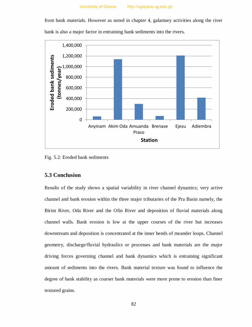
82

from bank materials. However as noted in chapter 4, galamsey activities along the river

bank is also a major factor in entraining bank sediments into the rivers.

Fig. 5.2: Eroded bank sediments

5.3 Conclusion

Results of the study shows a spatial variability in river channel dynamics; very active

channel and bank erosion within the three major tributaries of the Pra Basin namely, the

Birim River, Oda River and the Ofin River and deposition of fluvial materials along

channel walls. Bank erosion is low at the upper courses of the river but increases

downstream and deposition is concentrated at the inner bends of meander loops. Channel

geometry, discharge/fluvial hydraulics or processes and bank materials are the major

driving forces governing channel and bank dynamics which is entraining significant

amount of sediments into the rivers. Bank material texture was found to influence the

degree of bank stability as coarser bank materials were more prone to erosion than finer

textured grains.

0

200,000

400,000

600,000

800,000

1,000,000

1,200,000

1,400,000

Anyinam Akim Oda Amuanda Praso

Brenase Ejesu Adiembra

Ero

ded

ban

k se

dim

ents

(t

on

ne

s/ye

ar)

Station


83

Chapter Six

Catchment Scale Soil Loss and Sediment Yield Modelling

6.0 Introduction

Accelerated soil erosion is a worldwide problem because of its economic and environmental

impacts. To minimise the cost of field measurements of soil erosion and river sediment loads

many computer models have been developed and used to effectively estimate soil erosion which

aid in developing soil erosion management plans in many river basins. The Revised Universal

Soil Loss Equation (RUSLE) has been used in many countries, and input parameter data for

RUSLE have been well established over the years (Lim et al., 2005). In this chapter, the spatial

patterns in soil erosion and sediment yield in the Pra catchment has been assessed using the

revised universal soil loss equation (RUSLE) model. Research materials and methods used in

deriving the RUSLE parameters, how the parameters of RUSLE were integrated in GIS as well

as results of the RUSLE model are presented.

6.1 Materials and Methods

The revised universal soil loss equation (RUSLE) model has been used to model soil erosion in

the Pra Basin. It is defined as (Bonilla et al., 2010; Kouli et al., 2008; Renard et al., 1997);

A = RKLSCP ……………………. (6-1),

where; A is the soil loss (t/km2/yr); R the rainfall run-off erosivity factor (MJ mm km

2/h/yr); K

the soil erodibility factor; LS the slope steepness and slope length factor; C the vegetative cover

factor; and P the conservation practice factor are dimensionless.


84

Vector maps of parameters of equation 6-1 were generated and then converted to raster layers.

The raster maps were multiplied using raster calculator module in ArcGIS to generate soil

erosion and sediment yield maps of cells of varying magnitude of soil loss in the catchment

(Fig.6.1). The approach for deriving each parameter is discussed below.

Input Layers GIS Layers

DEM

Classify

RUSLE

Fig.6.1: Schematic chart of GIS applications to soil erosion mapping and the derivation of

Sediment Delivery Ratio, SDR (Modified from Mongkolsawat et al., 1994).

The rainfall erosivity index R measures the potential ability of rain to cause soil erosion. High

R values mean, high rainfall intensity with a higher potency of dislodging soils, hence the

expected soil erosion from the land surface and subsequent sediment yield will be high. Low R

Satellite Image

Topo Map

Soil Map

Rainfall Data

P factor

C factor

LS factor

K factor

R factor

Land cover map

Slope length

Slope

SDR Soil erosion

Sediment yield


85

value implies low rainfall intensity and run-off, consequently erosion and sediment yield will be

low. R factor map was derived from monthly EI30 values using the modified Fournier index

(MFI) (Shamshad, 2010);

R = 227MFI0.548

.............. (6-2).

The modified Fournier index (MFI) was estimated using total monthly erosive rainfall amounts

(Smithen and Schulze, 1982);

MFIe =

............. (6-3);

where: Pei, monthly erosive precipitation of month i, Pt, annual rainfall amount (mm). The

rationale for the choice of these equations is due to the fact that, they were developed in humid

tropics such as West Africa and Malaysia which are characterised by similar rainfall conditions

(intensity and amounts) like the study area. The mean annual erosivity map (isoerodent map) was

then produced in ArcGIS for the erosivity index (i.e, Re). Two erosivity maps were generated, 12

mm and 12.5 mm maps of total rainfall accumulation within 24 hours. Though an erosive event

has been defined as rainfall event with more than 12.50 mm of total rainfall accumulation

(Petkovšek and Mikoš, 2004; USDA-ARS, 2008a), however due to the thunderous nature of

humid tropical storms (large particle sizes, quantity and greater intensity) than the temperate

zones, 12.0 mm of total rainfall accumulation was also employed to determine its impact on soil

erosion.

K is a measure of the susceptibility of soil particles to detachment and transport by rainfall and

runoff (Stone and Hilborn, 2000). When K value is high, it implies deterioration in the physical

properties of the soil such as low organic matter, coarse soil texture, coarse granular structure

etc; thus the soil is more prone to erosion. Therefore, the higher the K value the more the soil is

prone to erosion. When K values are low, it implies an enhancement in the physical properties of


86

the soil such as increase in organic matter, fine soil texture, fine granular structure etc which

increases the cohesiveness of soil particles to resist erosion. This will result in low soil erosion

and sediment yield. The FAO K factor values of soils in the basin; (Table 6.1A) were used to

produce a raster layer of K factor map. Table 6.1B shows the susceptibility classes of soils.

LS measure the effects of topography on soil erosion and the steeper and longer the slope, the

higher is the risk for erosion and vice versa. The LS factor map for a cell area was computed with

equation 6-4 below in ArcGIS using upslope contributing area and slope gradient computed from

the digital elevation model (DEM) of the watershed. The DEM was generated from 1:50,000

scale contour map sourced from the Ghana Survey Department. The contours were interpolated

at 30 m pixel resolution using ‘topo to raster’ command in ArcGIS to create a hydrologically

correct DEM (e.g. Jain et al., 2010; Jain and Das, 2010). The generated DEM was further

reconditioned to a depressionless DEM using ‘fill sink’ command to determine the maximum

downhill slope and the flow direction which will maintain continuity of flow to catchment outlet

(e.g. Jain et al., 2010; Jain and Das, 2010). The slope (S) factor and flow accumulation were then

derived from the depressionless DEM and then LS map was generated based on equation 6-4 in

AcrGIS using the raster calculator module; (Jain et al., 2010; Jain and Das, 2010; Engel, 2003);

LS =

…………… (6-4);

Table 6.1A: K factor values of the soil types

Soil Type Area (Km2) K factor

Acrisols 18,328.8 0.00090

Alisols 213.4 0.00000

Arenosols 1.2 0.00000

Ferralsols 1.4 0.02800

Leptosols 206.2 0.00002

Lixisols 3,564.9 0.00000

Fluvisols 854.1 0.06460

Luvisols 11.0 0.00400

Table 6.1B: Soil erodibility classification

Soil erodibility

Classes

Soil K Factor

Very High >0.70

High 0.50-0.70

Moderate 0.25-0.50

Low 0.13-0.25

Very Low <0.13

Source: Hagos (2004)


87

where; As is upslope contributing area for overland grid per unit width normal to flow direction,

θ is the slope angle in degrees. On the basis of total length of stream channels of a 1:50,000

topographic map of the basin and the basin area, a channel initiation threshold value of 0.65 km2

was extracted and used to define channel cells (e.g. Jain and Das, 2010).

The cover management factor C is used to determine the relative effectiveness of soil and crop

management systems in terms of preventing soil loss. High C factor implies low vegetation cover

in the catchment, hence there is an increased opportunity for rainfall to detach sediments,

overland flow to scour and transport sediments, ultimately causing an increase in sediment

production and when C values are low, it implies good vegetative cover and erosion will be low.

Cover management factor map for C was determined using classified land cover and land use

map of landsat ETM + 2008 image (e.g. Jain et al., 2010; Jain and Das, 2010; Jain and Kothyari,

2000). The image was classified with reference to topographical maps, Google Earth and training

areas of sites taken in the field using a global positioning system (GPS). Seven land cover types

were classified using the maximum likelihood classifier module in Idrisi (Table 6.2). C factor

values suggested by Wischmeier and Smith (1978), were assigned to cells of the respective

classes as shown in Table 6.2.

The basin covers two landsat scenes (Table 6.3). The images were downloaded from the

Global Land Cover Facility website glovis.usgs.gov. This date was chosen based on the

availability of good satellite images covering the study area because due to thick cloud cover

most images were not suitable for usage. The 2008 images had no cloud cover, however due to

the failure of the Scan Line Corrector (SLC) of Landsat ETM+, there were gap marks on the

2008 images and these gaps were filled using the NASA gap filling software IDL 7.0 based on

1985/1986 images of the same locations. The images were merged and cropped to size using the


88

geographic coordinates of the basin. The classified image was then exported to ArcGIS, and

cropped to size using the vector layer of the drainage basin.

Table 6.2: Land cover types and cover management (C) factor values

Land Cover Type Area (km2) C Factor

Closed canopy 10,760.5 0.0001

Water bodies 3,109.4 0.0000

Built-ups & Barelands 1,160.6 0.3500

Open forest with shrubs & mixed arable tree

Crops

10,412.1 0.0003

Open savannah woodland with shrubs &

grassland

9,593.1 0.0020

Coastal scrub & grassland 9,855.9 0.0400

Bush fallows & cropland with natural

vegetation mosaic

4,929.0 0.5429

Table 6.3: Attributes of Landsat ETM+ 2008

Year & Image Scene Date of

Acquisition

Row Path Resolution Level of

Processing

2008 Landsat ETM+

(Kumasi and Pra’s

Mouth Scenes)

01/02/08 (for

both scenes)

055

and

056

194 30m L1T

P factor reflects the effects of soil erosion support practices that will reduce the amount and

rate of the water runoff and thus reduce the amount of erosion. Cross slope cultivation, contour

farming and strip cropping intercept flow paths and flow hydraulics of run-off. These soil

conservation practices will minimise soil erosion and sediment yield. P factor map was

determined in the field by finding out the kind of soil erosion management practices (i.e.

contouring, mulching, crop rotation etc) being practiced by land users (e.g. farmers, miners etc)

with reference to land cover classified landsat image of the catchment. Since in the study area, no

major conservation practices are followed, the P factor was taken as 1 for all land use and land

cover categories as majority of land areas have not been provided with any conservation support

(Jain and Das, 2010).


89

Soil erosion potential map of the basin was developed by multiplying the factor maps of K, LS,

C and P (Jain et al., 2010), whiles that of gross soil loss was determined by multiplying all the

derived factor maps of RUSLE (equation 6.1 and Fig.6.1).

The annual sediment yield of the watershed was estimated by multiplying soil loss map and

the sediment delivery ratio map (Fig.6.1) as expressed by equation 6.5 (Fistikoglu and

Harmancioglu, 2002):

Y = RKLSCP × SDR …………………………..(6-5);

where Y is the sediment yield (t/km2), SDR is the sediment delivery ratio, and RKLSCP is gross

erosion per unit area above a measuring point (Arekhi, 2008; Silva et al., 2010; USDA-ARS,

2008a).

SDR is defined as the ratio of sediment delivered at a given area in a stream system (sediment

yield) to the gross erosion or the fraction of gross erosion that is transported from a given

catchment in a given time interval. For each land cell, SDR depends upon several physical

characteristics of the watershed including surface roughness, land slope, soil hydrologic

conditions, and length of the travel path (flow length) to the stream and vegetative cover

(Kothyari and Jain, 1997).

The sediment delivery ratio for each cell i (SDRi) is a function of travel time (Jain and Kothyari

2000; Fu et al., 2006);

SDRi = exp(-βti) ................ (6.6);

where ti is the travel time (h) for each celli to the nearest channel cell down the drainage path and

β is a watershed-specific parameter regarded constant. The total travel time along a flow path is

expressed as (Jain and Kothyari, 2000);

ti =

.................. (6-7);


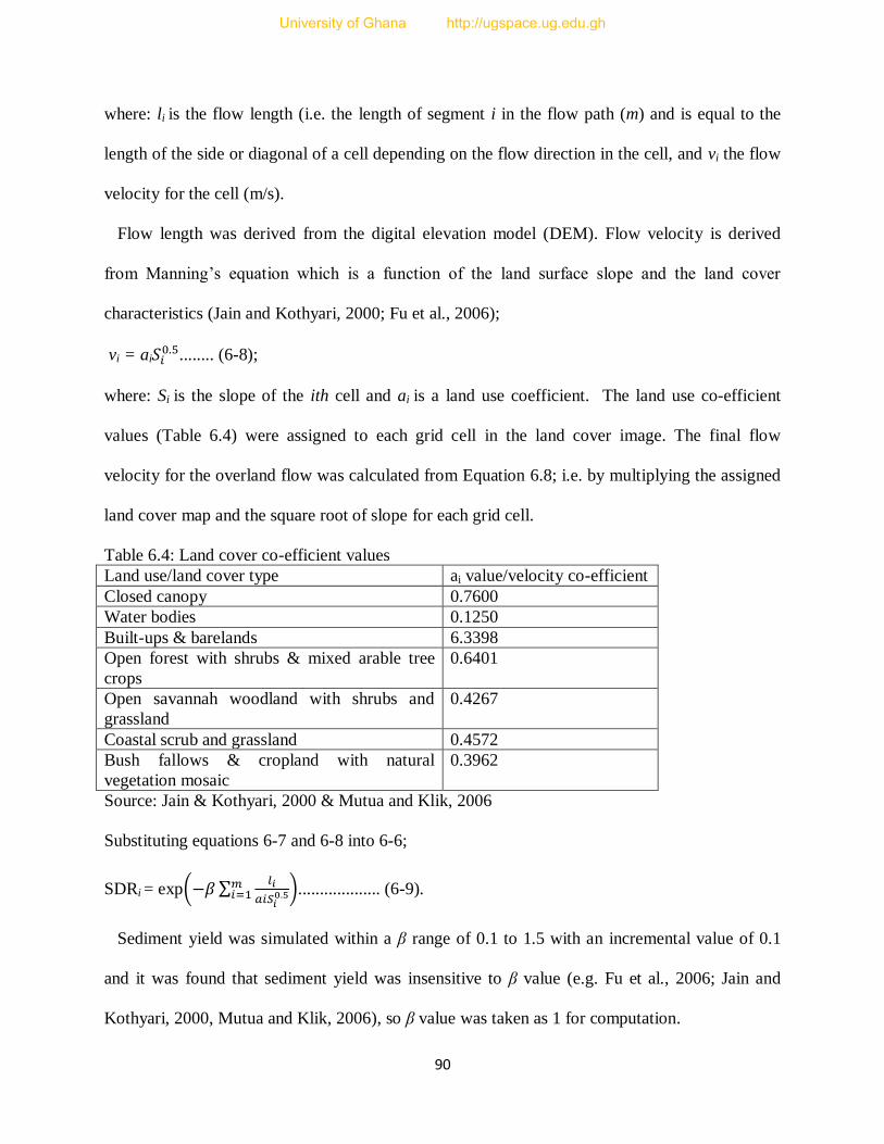
90

where: li is the flow length (i.e. the length of segment i in the flow path (m) and is equal to the

length of the side or diagonal of a cell depending on the flow direction in the cell, and vi the flow

velocity for the cell (m/s).

Flow length was derived from the digital elevation model (DEM). Flow velocity is derived

from Manning’s equation which is a function of the land surface slope and the land cover

characteristics (Jain and Kothyari, 2000; Fu et al., 2006);

vi = ai ........ (6-8);

where: Si is the slope of the ith cell and ai is a land use coefficient. The land use co-efficient

values (Table 6.4) were assigned to each grid cell in the land cover image. The final flow

velocity for the overland flow was calculated from Equation 6.8; i.e. by multiplying the assigned

land cover map and the square root of slope for each grid cell.

Table 6.4: Land cover co-efficient values

Land use/land cover type ai value/velocity co-efficient

Closed canopy 0.7600

Water bodies 0.1250

Built-ups & barelands 6.3398

Open forest with shrubs & mixed arable tree

crops

0.6401

Open savannah woodland with shrubs and

grassland

0.4267

Coastal scrub and grassland 0.4572

Bush fallows & cropland with natural

vegetation mosaic

0.3962

Source: Jain & Kothyari, 2000 & Mutua and Klik, 2006

Substituting equations 6-7 and 6-8 into 6-6;

SDRi = exp

................... (6-9).

Sediment yield was simulated within a β range of 0.1 to 1.5 with an incremental value of 0.1

and it was found that sediment yield was insensitive to β value (e.g. Fu et al., 2006; Jain and

Kothyari, 2000, Mutua and Klik, 2006), so β value was taken as 1 for computation.


91


The generated GIS layers of RUSLE for the determination of the magnitude of soil erosion in the

Pra Basin are shown in Figs. 6.2 – 6.6. Annual rainfall erosivity ranges from 456 – 1,181 and

553 – 1,166 MJ mm/ha/h/yr for the 12 and 12.5 mm erosivity events respectively with higher

intensities prevailing around Praso-Konongo-Juaso, a reflection of the climatic trend within the

basin (Fig.6.2 and Fig.6.3). Similar patterns in rainfall erosivity of the basin was observed in an

erosivity map produced by Oduro-Afriyie (1996) of Ghana and Roose (1977) of West Africa.

The 12 mm event map has the least and the highest erosivity values whiles the 12.5 mm map

least erosivity is higher than that of 12 mm event, because larger events were used to produce the

12.5 mm map, thus it will be more erosive due to the higher intensity of rainfall events. With

reference to the annual rainfall erosivity index (R) classification; R ≤2,452 low erosivity, 2,452 <

R ≤4,905 medium erosivity, 4,905 < R ≤ 7,357 medium-strong erosivity, 7,357 < R ≤ 9,810

strong erosivity, R > 9,810 very strong erosivity (Silva, 2004), the rainfall erosivity indices of the

basin are low.

The Pra catchment is underlain by 8 major soil types (alisols, acrisols, arenosols, ferralsols,

fluvisols, leptosols, lixisols and luvisols), with alisols, acrisols, lixisols having erodibility values

of 0 and fluvisols being most erodible (0.0646 t h MJ-1

mm-1

) (Fig.6.4). All these soils are

classed as having very low erodibilities when exposed with the most erodible types being

concentrated in the river valleys (Table 6.1B).

Forest reserves making up the closed canopy had the best vegetative cover whiles urban

centres and barelands (mine sites) had sparse vegetative cover (Fig.6.6). Over 81% of the

catchment was protected by vegetative cover composing of forest reserves, open/secondary

growth, savannah and coastal scrub/grassland with only about 22% being covered by


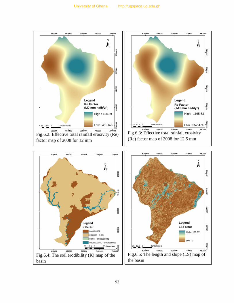
92

Fig.6.2: Effective total rainfall erosivity (Re)

factor map of 2008 for 12 mm

620000

620000

660000

660000

700000

700000

740000

740000

780000

780000

55

00

00

55

00

00

60

00

00

60

00

00

65

00

00

65

00

00

70

00

00

70

00

00

75

00

00

75

00

00

±


Legend

Re Factor(MJ mm ha/h/yr)

High : 1180.9

Low : 455.675

Fig.6.3: Effective total rainfall erosivity

(Re) factor map of 2008 for 12.5 mm

620000

620000

660000

660000

700000

700000

740000

740000

780000

780000

55

00

00

55

00

00

60

00

00

60

00

00

65

00

00

65

00

00

70

00

00

70

00

00

75

00

00

75

00

00

±


Legend

Re Factor ( MJ mm ha/h/yr)

High : 1165.63

Low : 552.474

Fig.6.5: The length and slope (LS) map of

the basin

620000

620000

660000

660000

700000

700000

740000

740000

780000

780000

55

00

00

55

00

00

60

00

00

60

00

00

65

00

00

65

00

00

70

00

00

70

00

00

75

00

00

75

00

00

±


Legend

LS Factor

High : 108.611

Low : 0

Fig.6.4: The soil erodibility (K) map of the

basin

620000

620000

660000

660000

700000

700000

740000

740000

780000

78000055

00

00

55

00

00

60

00

00

60

00

00

65

00

00

65

00

00

70

00

00

70

00

00

75

00

00

75

00

00±

Kilometers25 0 2512.5

Legend

K Factor

0 - 0.00002

0.00002 - 0.004

0.004 - 0.028000001

0.028000001 - 0.064599998


93

bushes/cropland and built-ups/barelands.

The length and steepness of slopes is high at the source of the basins such as the Atewa Forest

Reserve watershed and the Ashanti Mampong-Kwahu Scarps which serves as the source of the

Pra, Birim and Oda Rivers, and around Lake Bosomtwi due to the mountain formations, whereas

the LS of the other parts of the basin particularly the southern part is very low (Fig.6.5). Much of

the basin area is characterised by low values of LS and transport of eroded materials will be very

limited owing to the low gradient.

Fig.6.7 shows areas of varying KLSCP values and hence the soil erosion potential in the

different cells of the river catchment. Values of potential soil loss ranged between 0 and 0.59

tonnes/year. Overlay of Fig.6.6 on slope, rainfall erosivity and landuse/landcover maps revealed

that higher cell values of soil erosion coincide with steep slopes, higher rainfall intensity zones

Fig.6.7: Soil erosion potential map of the

basin

620000

620000

660000

660000

700000

700000

740000

740000

780000

780000

55

00

00

55

00

00

60

00

00

60

00

00

65

00

00

65

00

00

70

00

00

70

00

00

75

00

00

75

00

00

80

00

00

80

00

00

±


Legend

KLSCP

High : 0.593519

Low : 0

Fig.6.6: Cover management factor (C) map

derived from satellite image classification

600000

600000

650000

650000

700000

700000

750000

750000

56

00

00

56

00

00

62

00

00

62

00

00

68

00

00

68

00

00

74

00

00

74

00

00

80

00

00

80

00

00

±

25 0 2512.5 km

Legend

C Factor

0 - 0.0001

0.0001 - 0.0002

0.0002 - 0.004

0.004 - 0.542900026


94

and cells of urban centres. High values of this term indicate a higher potential of soil erosion in

those cells and vice-versa.

Figure 6.8 and 6.9 illustrate the gross soil erosion for the annual rainfall year 2008. Estimated

annual soil loss from a cell ranged from 0 to 3.91 and 0 – 3.96 t/ km2/yr for both 12 and 12.5 mm

events with a mean of 0.001 t/ km2/yr and a standard deviation of 0.02 t/ km

2/yr. The relative

higher soil erosion by 12.5 mm is attributable to the higher intensity of the event. Generally, the

catchment is characterised by low soil loss risk based on the four classes of basin soil loss

proposed by FAO (1967, cited by Silva et al., 2010) in t/km2/yr: (a) < 0.10 = very low, (b) 0.10–

0.50 = moderate, (c) 0.50–2 = high, and (d) >2 = very high. The low soil erosion is due to the

well protected landscape by the vegetative cover, and low gradient of the topography. Zones

susceptible to moderate-high erosion risks are very few and these occur in built-ups, exposed

landscapes (galamsey areas) and also along steep slopes and within the river valleys underlain by

fluvisols which are very susceptible to erosion.

The highest soil loss occurs in river valleys and the erosion tends to increase downstream as a

result of increase in flow accumulation down slope from the source towards catchment outlet.

Most urban centres are characterized by moderate soil erosion and this is due to the exposed

nature of these urban landscapes (unpaved and not grassed). High run-offs generated during

rainfalls cause serious urban erosion creating rills/gullies and entraining sediments into

gutters/gullies which are channelled into nearby streams and rivers. These results are akin to

other RUSLE/USLE model estimates of soil erosion in a number of basins in Brazil all in the

tropics. Annual soil loss was estimated to be 0-0.032 and 0-0-2.93 in Guaraíra and Tapacurá

catchments (Silva et al., 2007; 2010). Field investigations confirm the model results, that there is


95

SDR generally decreases with increasing basin

Fig.6.8: Gross soil erosion map of 12 mm

erosive event

620000

620000

660000

660000

700000

700000

740000

740000

780000

780000

55

00

00

55

00

00

60

00

00

60

00

00

65

00

00

65

00

00

70

00

00

70

00

00

75

00

00

75

00

00

±


Legend

Soil Erosion

t/km sq/yr

High : 3.91

Low : 0

Fig.6.11: Sediment yield map of 12 mm

erosive event

620000

620000

660000

660000

700000

700000

740000

740000

780000

780000

55

00

00

55

00

00

60

00

00

60

00

00

65

00

00

65

00

00

70

00

00

70

00

00

75

00

00

75

00

00

±


Legend

Sediment yield

t/km sq/yr

High : 1.94

Low : 0

Fig.6.10: Sediment delivery ratio map of the

basin

620000

620000

660000

660000

700000

700000

740000

740000

780000

780000

55

00

00

55

00

00

60

00

00

60

00

00

65

00

00

65

00

00

70

00

00

70

00

00

75

00

00

75

00

00

±


Legend

SDR values

High : 1

Low : 0

Fig.6.9: Gross soil erosion map of 12.5 mm

erosive event

620000

620000

660000

660000

700000

700000

740000

740000

780000

780000

55

00

00

55

00

00

60

00

00

60

00

00

65

00

00

65

00

00

70

00

00

70

00

00

75

00

00

75

00

00

±


Legend

Soil Erosion

t/km sq/yr

High : 3.96

Low : 0


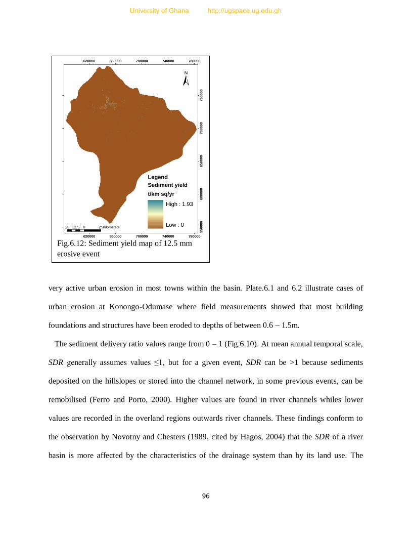
96

very active urban erosion in most towns within the basin. Plate.6.1 and 6.2 illustrate cases of

urban erosion at Konongo-Odumase where field measurements showed that most building

foundations and structures have been eroded to depths of between 0.6 – 1.5m.

The sediment delivery ratio values range from 0 – 1 (Fig.6.10). At mean annual temporal scale,

SDR generally assumes values ≤1, but for a given event, SDR can be >1 because sediments

deposited on the hillslopes or stored into the channel network, in some previous events, can be

remobilised (Ferro and Porto, 2000). Higher values are found in river channels whiles lower

values are recorded in the overland regions outwards river channels. These findings conform to

the observation by Novotny and Chesters (1989, cited by Hagos, 2004) that the SDR of a river

basin is more affected by the characteristics of the drainage system than by its land use. The

Fig.6.12: Sediment yield map of 12.5 mm

erosive event

620000

620000

660000

660000

700000

700000

740000

740000

780000

780000

55

00

00

55

00

00

60

00

00

60

00

00

65

00

00

65

00

00

70

00

00

70

00

00

75

00

00

75

00

00

±


Legend

Sediment yield

t/km sq/yr

High : 1.93

Low : 0


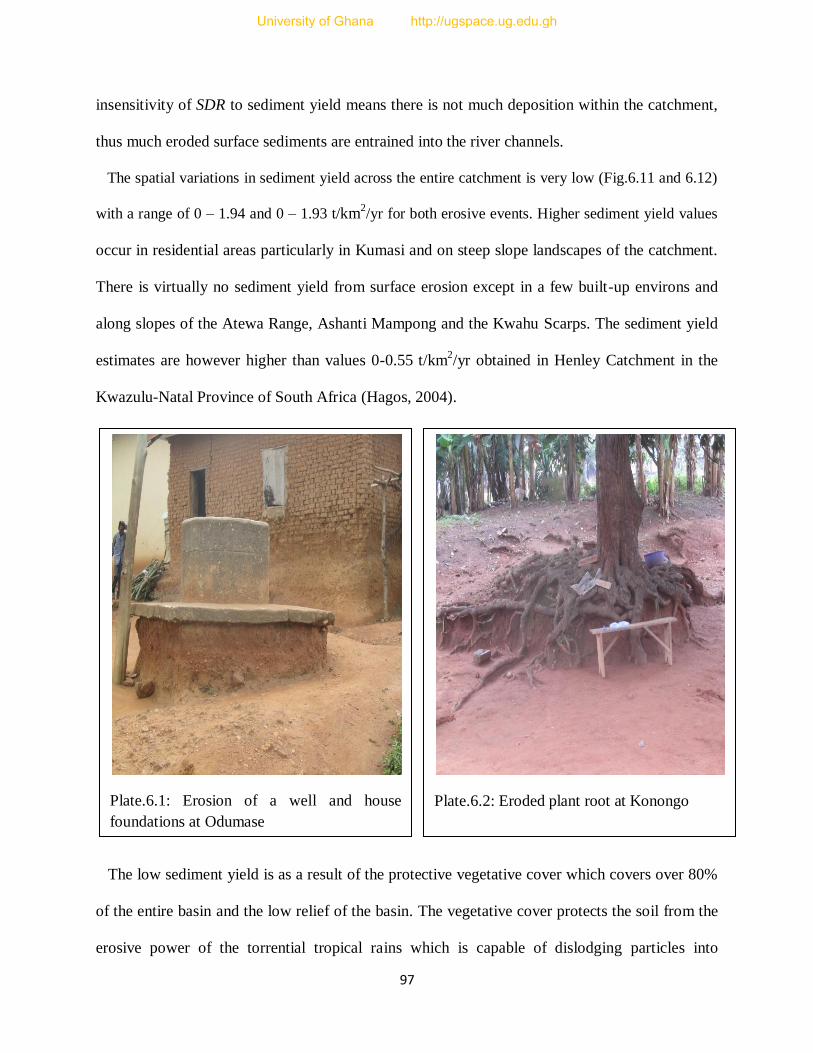
97

insensitivity of SDR to sediment yield means there is not much deposition within the catchment,

thus much eroded surface sediments are entrained into the river channels.

The spatial variations in sediment yield across the entire catchment is very low (Fig.6.11 and 6.12)

with a range of 0 – 1.94 and 0 – 1.93 t/km2/yr for both erosive events. Higher sediment yield values

occur in residential areas particularly in Kumasi and on steep slope landscapes of the catchment.

There is virtually no sediment yield from surface erosion except in a few built-up environs and

along slopes of the Atewa Range, Ashanti Mampong and the Kwahu Scarps. The sediment yield

estimates are however higher than values 0-0.55 t/km2/yr obtained in Henley Catchment in the

Kwazulu-Natal Province of South Africa (Hagos, 2004).

The low sediment yield is as a result of the protective vegetative cover which covers over 80%

of the entire basin and the low relief of the basin. The vegetative cover protects the soil from the

erosive power of the torrential tropical rains which is capable of dislodging particles into

Plate.6.1: Erosion of a well and house

foundations at Odumase

Plate.6.2: Eroded plant root at Konongo


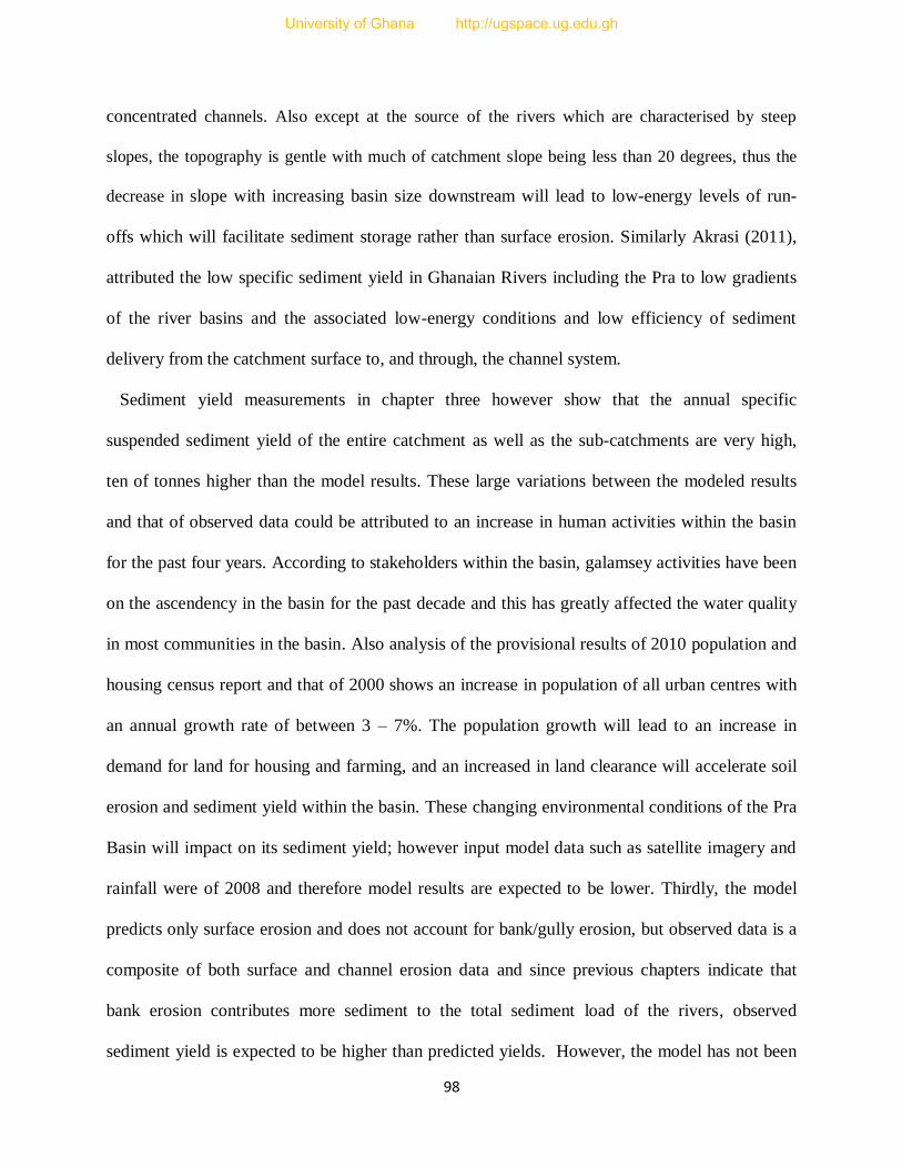
98

concentrated channels. Also except at the source of the rivers which are characterised by steep

slopes, the topography is gentle with much of catchment slope being less than 20 degrees, thus the

decrease in slope with increasing basin size downstream will lead to low-energy levels of run-

offs which will facilitate sediment storage rather than surface erosion. Similarly Akrasi (2011),

attributed the low specific sediment yield in Ghanaian Rivers including the Pra to low gradients

of the river basins and the associated low-energy conditions and low efficiency of sediment

delivery from the catchment surface to, and through, the channel system.

Sediment yield measurements in chapter three however show that the annual specific

suspended sediment yield of the entire catchment as well as the sub-catchments are very high,

ten of tonnes higher than the model results. These large variations between the modeled results

and that of observed data could be attributed to an increase in human activities within the basin

for the past four years. According to stakeholders within the basin, galamsey activities have been

on the ascendency in the basin for the past decade and this has greatly affected the water quality

in most communities in the basin. Also analysis of the provisional results of 2010 population and

housing census report and that of 2000 shows an increase in population of all urban centres with

an annual growth rate of between 3 – 7%. The population growth will lead to an increase in

demand for land for housing and farming, and an increased in land clearance will accelerate soil

erosion and sediment yield within the basin. These changing environmental conditions of the Pra

Basin will impact on its sediment yield; however input model data such as satellite imagery and

rainfall were of 2008 and therefore model results are expected to be lower. Thirdly, the model

predicts only surface erosion and does not account for bank/gully erosion, but observed data is a

composite of both surface and channel erosion data and since previous chapters indicate that

bank erosion contributes more sediment to the total sediment load of the rivers, observed

sediment yield is expected to be higher than predicted yields. However, the model has not been


99

able to capture the impact of illegal small scale mining activities in the basin consequently the

development of a model that is capable of capturing both surface and concentrated soil erosion

should be explored in the future.

Results of the two models, the 12 mm and 12.5 mm erosive events do not vary much, the 12

mm modelled results is just about 0.5% higher than that of 12.5 mm, hence the use of any of

these events in predicting soil erosion will produce similar results which will not be statistical

different from each other hence any of these events can be adopted for soil erosion and sediment

yield mapping in the basin. The level of accuracy of each event could only be ascertained if the

model had been calibrated, but due to the time lag between the observed data and the model

results, and considering the extent of increase in human activities within the basin over the past

four years as well as the lack of current rainfall and land cover/use data of the basin, the use of

the observed that in calibrating the model could result in greater errors and high levels of

uncertainty.

6.3 Sediment Yield Sensitivity Analysis

Sensitivity analysis is the study used to ascertain how a given model output depends upon the

information (input data) fed into it, upon its structure and upon the framing assumptions made to

build it (Saltelli et al., 2000; Hagos, 2004). Sensitivity analysis is used to increase the confidence

in the model and its predictions, by providing an understanding of how the model responds to

changes in the input parameters (Saltelli et al., 2000; Hagos, 2004).

In this research, a sensitivity analysis of RULSE parameters (R, K, C, LS, P and SDR) was

done to measure the sensitivity of the model prediction to a change in the variable value (Hagos,

2004). The means and standard deviations of each of the input RULSE data layers were extracted


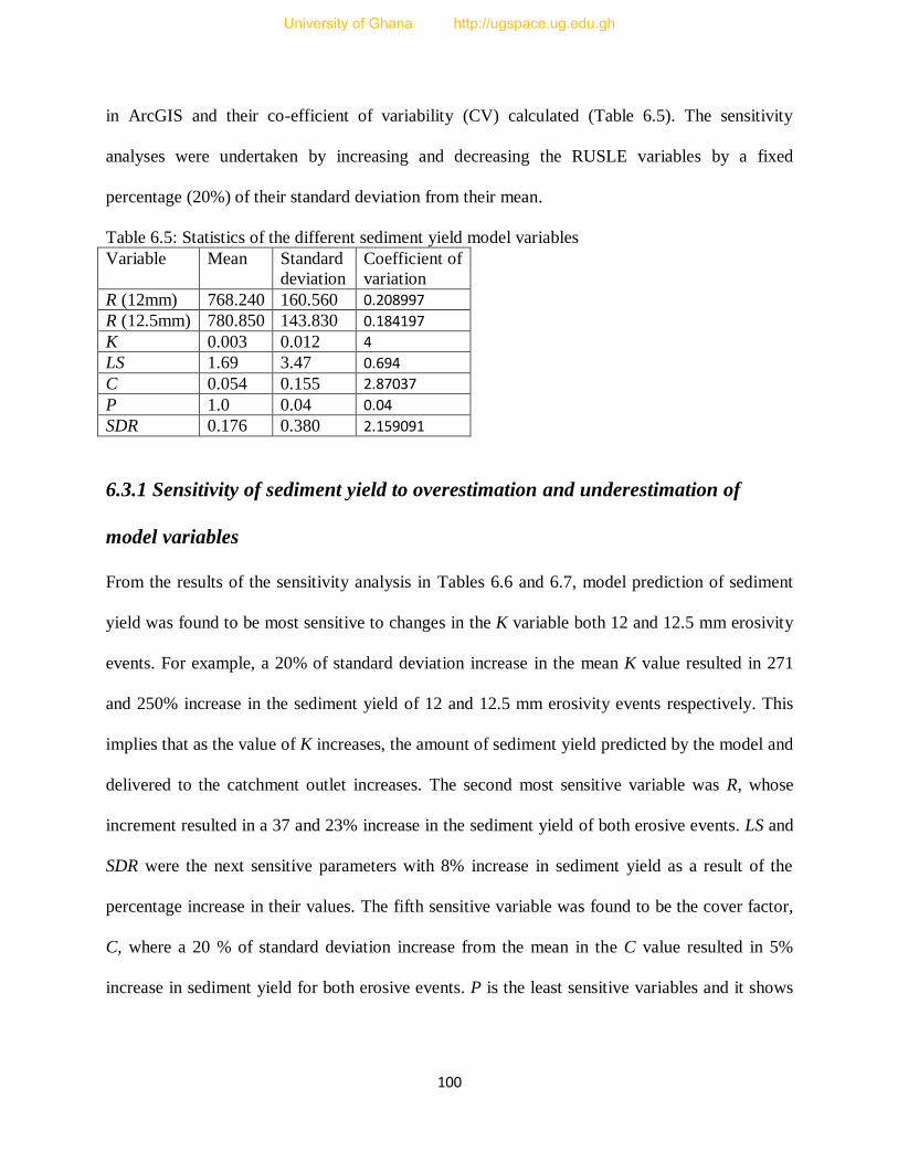
100

in ArcGIS and their co-efficient of variability (CV) calculated (Table 6.5). The sensitivity

analyses were undertaken by increasing and decreasing the RUSLE variables by a fixed

percentage (20%) of their standard deviation from their mean.

Table 6.5: Statistics of the different sediment yield model variables

Variable Mean Standard

deviation

Coefficient of

variation

R (12mm) 768.240 160.560 0.208997

R (12.5mm) 780.850 143.830 0.184197

K 0.003 0.012 4

LS 1.69 3.47 0.694

C 0.054 0.155 2.87037

P 1.0 0.04 0.04

SDR 0.176 0.380 2.159091

6.3.1 Sensitivity of sediment yield to overestimation and underestimation of

model variables

From the results of the sensitivity analysis in Tables 6.6 and 6.7, model prediction of sediment

yield was found to be most sensitive to changes in the K variable both 12 and 12.5 mm erosivity

events. For example, a 20% of standard deviation increase in the mean K value resulted in 271

and 250% increase in the sediment yield of 12 and 12.5 mm erosivity events respectively. This

implies that as the value of K increases, the amount of sediment yield predicted by the model and

delivered to the catchment outlet increases. The second most sensitive variable was R, whose

increment resulted in a 37 and 23% increase in the sediment yield of both erosive events. LS and

SDR were the next sensitive parameters with 8% increase in sediment yield as a result of the

percentage increase in their values. The fifth sensitive variable was found to be the cover factor,

C, where a 20 % of standard deviation increase from the mean in the C value resulted in 5%

increase in sediment yield for both erosive events. P is the least sensitive variables and it shows


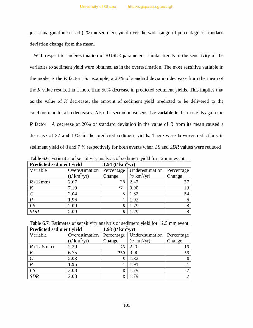
101

just a marginal increased (1%) in sediment yield over the wide range of percentage of standard

deviation change from the mean.

With respect to underestimation of RUSLE parameters, similar trends in the sensitivity of the

variables to sediment yield were obtained as in the overestimation. The most sensitive variable in

the model is the K factor. For example, a 20% of standard deviation decrease from the mean of

the K value resulted in a more than 50% decrease in predicted sediment yields. This implies that

as the value of K decreases, the amount of sediment yield predicted to be delivered to the

catchment outlet also decreases. Also the second most sensitive variable in the model is again the

R factor. A decrease of 20% of standard deviation in the value of R from its mean caused a

decrease of 27 and 13% in the predicted sediment yields. There were however reductions in

sediment yield of 8 and 7 % respectively for both events when LS and SDR values were reduced

Table 6.6: Estimates of sensitivity analysis of sediment yield for 12 mm event

Predicted sediment yield 1.94 (t/ km2/yr)

Variable Overestimation

(t/ km2/yr)

Percentage

Change

Underestimation

(t/ km2/yr)

Percentage

Change

R (12mm) 2.67 38 2.47 27

K 7.19 271 0.90 13

C 2.04 5 1.82 -54

P 1.96 1 1.92 -6

LS 2.09 8 1.79 -8

SDR 2.09 8 1.79 -8

Table 6.7: Estimates of sensitivity analysis of sediment yield for 12.5 mm event

Predicted sediment yield 1.93 (t/ km2/yr)

Variable Overestimation

(t/ km2/yr)

Percentage

Change

Underestimation

(t/ km2/yr)

Percentage

Change

R (12.5mm) 2.39 23 2.20 13

K 6.75 250 0.90 -53

C 2.03 5 1.82 -6

P 1.95 1 1.91 -1

LS 2.08 8 1.79 -7

SDR 2.08 8 1.79 -7


102

by 20% of the standard deviation of their values. C and P factors were the fifth and sixth

sensitive variables and their level of sensitive is very low. Generally, overestimated model was

much sensitive to sediment yield prediction and the level of sensitivity was much higher with 12

mm rainfall erosivity than with 12.5 mm index. The most sensitive factors in sediment yield

prediction of the Pra Basin are K and R whiles the least sensitive variables are C, P, LS and SDR.

Therefore in prediction sediment yield in the basin, K and R parameter values need to be

estimated with very good accuracy and so be given more attention in estimating their values as

errors in their input data will have much impact on the outcome of the results. However errors in

the input data of the C, P, LS and SDR parameters will have less impact on the output results.

6.4 Conclusion

Given the elements and processes prevailing in the basin in 2008, surface soil erosion and

sediment yield is very low but this condition could degenerate into very severe surface soil

erosion if the current state of land degradation, particularly by galamsey activities are allowed to

continue. These results reflect findings of chapter four which indicates that much of fluvial

sediment transported is from bank materials. However, results of the sensitivity analyses shows

variables such as K, and R to be very sensitive to predicted sediment yield particularly when

overestimated. This calls for high accuracy in the estimation of K, and R input data to ensure

precision of model results. A synthesis of the various chapters will be discussed in the next

chapter.


103

Chapter Seven

A Synthesis of Results, Conclusion and Recommendations

7.0 Introduction

Soil erosion and sediment transport are subject to highly complex processes that are very

cumbersome to study; because these processes and their interactions with each other influence

soil loss and sediment yield (Hagos, 2004). Owing to the importance of these processes a number

of models that use these processes to simulate catchment soil loss and sediment yield have been

developed over the years (Hagos, 2004). In this study, soil erosion and sediment yield patterns

were modelled using the revised universal soil loss equation. In situ sediment yield and bank

erosion measurements were also undertaken to ascertain the level of sediment discharge in the

river basin and channel stability. Lastly, a finger print approach was also employed to determine

the source of sediments whether from bank materials or surface soils. As a concluding chapter,

the relationship between findings of the various chapters have been synchronised and discussed.

Other sections of the chapter include a discussion on the policy implication of the findings,

limitations/challenges encountered in the study, conclusion and recommendations for policy

makers and future studies.

7.1 The Nexus between Field Measurements and Modelling of Soil Loss and

Sediment Delivery

This study was undertaken in the Pra River Basin to assess the level of soil erosion/sediment

yield and bank erosion using the revised universal soil loss equation (RUSLE) and field data

collection. The model was able to determine the spatial variability in soil erosion and sediment


104

yield. Model results showed that the Pra Basin was characterized by a low surface soil erosion

and sediment yield generation owing to the relatively low risk factors such as low topography of

the landscape and the thick vegetative cover. Thus soil erosion and sediment yield were

concentrated in exposed landscapes such as urban centres and steep slopes characterized by

intense rainfall activity. The model could not be validated as it predicts only surface sediments

and does not account for channel/gulley erosion and sediment yield. Therefore it will be

inappropriate to use sediment load or sediment yield measurements which consist of both surface

and bank/gully/channel eroded sediments for validating the model.

For instance the sister model USLE which does not also account for gully/channel erosion was

used by Simanton et al. (1980, cited by Lim et al., 2005) to predict soil loss of four watersheds.

They found that USLE estimated soil losses matched reasonably for two watersheds that had no

gullies or significant alluvial channels, while USLE results did not match well for the other two

watersheds with significant gullies and channels. These results indicate that USLE should not be

applied to large watersheds, experiencing significant gully and channel erosion (Lim et al.,

2005). Also predicted soil loss was less than the measured sediment yield for two basins using

MUSLE (Modified Universal Soil Loss Equation) and for three basins using RUSLE (Erskine et

al.,2002), because they do not account for gully erosions.

Besides, the satellite image and rainfall data used for the model was that of 2008 and the

sediment yield studies were carried out in 2012 so it will not be appropriate to use sediment yield

data of 2012 to calibrate a model predicting sediment yield of 2008 in the midst of lot of

environmental changes taking place within the basin. As indicated in previous chapters, the

activities of the illegal small scale mining has increased tremendously over the past decade and

this will impact greatly on sediment yield hence sediment transport in 2012 is expected to be


105

higher than that of 2008 and this also explains the variability in sediment yield between observed

and predicted.

Results of sediment yield measurements however show that the suspended sediment yield of

the sub-catchments and the main Pra system are very high. Suspended sediment discharge

indicates high suspended sediment transported throughout the season even at low flows. This

high variability in sediment yield between model results and that of observed data implies that,

there is more bank erosion than surface erosion within the basin and since the model does not

account for bank erosion, sediments from bank materials are not captured in the modelling. This

observation is buttressed by sediment source tracking analyses which showed that bank sediment

materials were more dominant tracers than surface soils in all the tributaries studied including the

main Pra catchment. Bank materials accounted for over 60% of suspended sediment loads in all

sub-basins, and this explains the great variation between the model results and observed field

sediment yield data measured. The strong positive correlation between sediment yield and basin

area is also indicative of high fluvial sediment transport from the sources of the rivers through

the basin system to the outlet.

These high discharges are attributable to human activities along the river corridor, most likely

illegal alluvial gold mining activities taking place within the Pra Basin particularly those

undetaken in the rivers. As discussed in the previous chapters, these activities result in the

continuous entrainment of sediments from the river bank, mine wastes and the remobilzation of

deposited bed materials. Though surface sediments entrainment into streams are lower than bank

materials, there is the need to manage land use activities in these basins to avoid over

exploitation/degradation of the vegetation especially in the upsurge of mining activities coupled

with farming. This is because the sensitivity analyses showed that predicted sediment yield was


106

very sensitive to C variable especially when the vegetative cover is reduced. The magnitude of

the sediment delivery ratio for a particular basin is influenced by a wide range of

geomorphological and environmental factors including the nature, extent and location of the

sediment sources, relief and slope characteristics, the drainage pattern and channel conditions,

vegetation cover, land use and soil texture (Walling, 1983). High sediment yields are known to

pertain in smaller basins where sediments from source areas are easily moved into channels or

downstream without significant deposition because the channel network of a small basin is

generally constituted of channels having narrow cross sections and short channel lengths

(Erskine et al. 2002; Ferro and Porto, 2000). High yields are also common in catchments that

have either been extensively disturbed by agriculture or have experienced high density gulling

(e.g. Erskine et al., 2002).

Though there is active bank erosion by hydraulic processes of flow which also contributes to

sediments in the rivers, the proportion of sediment emanating from these processes is small as

compared to the galamsey activity. This is because bank erosion measurements showed that

much bank erosion occurred during high flows, but the relatively high sediment discharges that

occurred during low flows as revealed by the suspended sediment concentration values cannot be

attributed to the hydraulic erosional processes, but galamsey. Apart from those who operate on

the rivers, there are other operators who dig pits which are often along the bank of the river or a

stream and they create channels through which the mine waste is discharged into the rivers, so

even at low flows there are thick plumes of sediments from mine waste water that are discharged

into the streams/rivers. In communities where these galamsey activities are on-going, they

indicated that due to the large sediment discharge and chemicals used in these operations, the

water has become too polluted and they cannot use it any longer. According to them, the


107

situation has even led to the reduction in stock of aquatic species such as fish and crabs which

they used to depend on for food.

The implication of the level of sediment load and transport pattern in the entire Pra Basin is

that, it poses a great threat to the sustainability of the dams built on the rivers and water quality

of the rivers in general. Dams built on these rivers (e.g. Owabi Dam, Barekese Dam and Brimsu

Dam etc) are all silting up rapidly and Government has to spend lot of money in de-silting them

to ensure potable water supply to communities within the basin. Ghana Water Company Limited

is always complaining of the increasing cost of treating water for potable purposes along these

rivers due to the high sedimentation levels of the water bodies. Also sediment load affects water

turbidity. Turbidity determines the degree of scattering or absorption of light in the water and

thus influences water temperature and the growth of aquatic plants and algae which can increase

water loss (evapo-transpiration) or cause eutrophication which will worsen the water stress

situation of communities in these basins.

From the above syntheses, it is obvious that sediment yield prediction within the Pra Basin

using the RUSLE does not complement data from in situ sediment yield measurements due to the

large amount of sediments generated within river channels. The inability of RUSLE to capture

sediments generated from concentrated flow channels is a major limitation of the model and

future research in modelling sediment yield within the basin should consider addressing this

problem. However, as has been noted in literature the model is user friendly as its data input is

very simple to generate and can be incorporated into GIS to give a spatial dimension to the

phenomena understudy. Though the field measurement of the sediment yield is reflective of the

trends of sediment transport within the catchment, in situ data collection of sediment yield has

been observed to be expensive and time consuming, consequently the application of a model


108

capable of capturing concentrated sediment transport will make sediment yield assessment

within the basin faster, easier, cheaper and more convenient.

7.2 Limitations of the study

In the collection and analysis of data for this project a number of setbacks were encountered

which need to be enumerated to guide future studies of this kind. This included the lack of

certain logistics and data.

One major challenge that confronted this study was the unavailability of good satellite images

covering the study area to enable a decadal/temporal modelling of soil erosion and sediment

yield of the basin. Most of the available Landsat images had much cloud cover and could not be

used for the study except that of the 2008. Thus it was impossible to model soil loss and

sediment yield between different periods to determine trends in these processes within the basin.

Another limitation of the model is its inability to model bank/gully erosion of channels and as

discussed in literature it is unsuitable for large basins. As revealed by sediment yield

measurements and source analyses, much of the fluvial sediments in transport are from bank

materials hence an accurate sediment yield model of the Pra Basin will require a model that

could also predict bank erosion.

A study of this kind required the use of a boat to facilitate movement along the river for a

better assessment of processes and field data collection. The researcher could not however

acquire/access this facility for lack of funds; consequently field measurements of bank erosion

and bank sediment source analysis had to be restricted to the sub-basins whose channels were

easily accessible due to the small volumes of water they carried. Though certain sections of the


109

river were undergoing active channel erosion, they were not accessible for lack of a boat to

navigate these courses. This therefore limited the number of monitoring sites of bank erosion.

At some stations such as Sekyere Heman and Adwumain, stream gauges were vandalized by

galamsey operators and at Akim Oda, the readings of lower gauge staffs were also worn-out and

not legible. Readings taken during these stages were only estimates and in Adwuman sampling

was impossible because all gauges had been removed as a result of illegal mining activities along

the river bank. Also at Sekyere Heman some gauge staffs had also been removed by the illegal

miners and this affected gauge readings at those stages of flow. These challenges were known to

the Ghana Hydrological Services Department through their gauge readers, but the Service

complained that, they lacked funds to maintain the defaced gauges and also had no control over

the illegal miners. Insufficient funding from the state also affected their ability to undertake flow

measurements regularly.

Erosion pins unlike PEEP is incapable of determining the magnitude, timing, spatial variability

and dynamics of erosion events, consequently spatio-temporal comparison of bank erosion with

respect to rainfall events/flows was impossible. The lack of bank erosion monitoring at high

resolution intervals using PEEPS prevented a better characterization of the fluvial erosion

processes with hydrograph events. Thus bank erosion could not be associated with fluvial events

and processes and the detection of critical erosion events during the period of observation. That

is the timing and magnitude of specific erosion events could not be captured. PEEP could not be

deployed for the study for lack of funds to purchase the equipment and there was none for hiring

as well.

Sediment concentrations were determined using both the integrated and dip samplings with the

dip samples being corrected by a correction factor of the integrated samples. This will definitely


110

result in some marginal errors in the concentration levels. Also sampling was not done strictly

according to the hydrological regime of flow due to the small number of visiting times, thus

certain critical flows were missed irrespective of the number of samples taken particularly in

stations were people could not be engaged to undertake dip sampling. Nevertheless, though a

strict hydrological regime was not followed, the field work was scheduled in such a way that

more samples were taken during the rising and peak stages of the season than the falling stages

and this could provide a fair idea of the sediment discharge regime of the catchments. Also error

margins are said to be low with larger basin sizes, so the expected associated errors related to

sediment rating curves will be low (e.g. Walling, 1977a and 77b; Horowitz, 2003).

As indicated earlier, some bank erosion sites were vandalised due to the illegal mining

activities and this prevented the empirical assessment of the level of bank erosion at those

stations.

7.3 Conclusion

The study shows a very effective combination of spatial data of RUSLE parameters into GIS in

mapping the spatial patterns in soil erosion and sediment yield. Simulated results showed that

soil loss and sediment yield for 2008 in the Pra were generally low with zones susceptible to

moderate-high erosion risks being few and these occurred in built-ups, high rainfall intensity and

exposed landscapes (galamsey) areas and also along steep slopes and within the river valleys

underlain by fluvisols which are very susceptible to erosion. Results of sediment yield derived

from the integration of RUSLE into GIS gives a vivid spatial dimensions in sediment yield in the

Pra Basin, however due to the unavailability of observed data the model could not be calibrated

and validated. There is therefore the need to calibrate and validate the RUSLE model in the


111

future with respect to its application in the basin. The low erosion and sediment yield risk

patterns are as a result of the well protected nature of the landscape by vegetative cover;

consequently, measures must be put in place by state institutions to maintain a good vegetative

cover of the basin especially in the light of serious threat from galamsey operations. Urban

greening to protect the soil and the construction of good drains to carry run-off should also be

encouraged by District Assemblies to protect the soil from urban erosion. Results of sensitivity

analyses showed variables such as K, and R to be very sensitive to predicted sediment yield

particularly when overestimated. This calls for high accuracy in the estimation of K, and R input

data to ensure precision of model results.

The suspended sediment yield of the Pra Basin has been found to be higher than most tropical

rivers including those in Ghana and illegal gold mining is the major force entraining large

volumes of sediments into the rivers. These high yields are negatively impacting on the ability of

Ghana Water Company to produce and distribute potable water to communities within the Pra

Catchment. The deteriorative quality of the water is also causing aquatic life to perish.

Communities are therefore getting stressed in terms of good quality water supply and protein

need from fish.

A fingerprinting technique involving 210

Pb analyses showed that a greater percentage of fluvial

sediments are emanating from bank materials. Human activities (galamsey) and bank erosion are

the driving forces injecting bank sediments into the rivers. Field investigations and sediment

yield results however indicate that much of the bank sediment injection is as a result of galamsey

activities. Bank erosion studies revealed that, there is much channel instability along most cross

sections particularly along meander bends and confluences. Other sections of river channels


112

characteristic of inner curves of meanders and banks of cohesive particles sizes and good

vegetative cover are very stable.

7.4 Recommendations

In view of the lack of decadal modeling of soil erosion and sediment yield of the basin, it is

recommended whenever it is possible (availability of two time period of satellite images) any

study of this kind should attempt a temporal analyses of the sediment yield to decipher changing

patterns in soil erosion and sediment yield in the basin. Also due to the current high intensity of

human activities along and within the river banks which is entraining more sediments into the

rivers than surface processes, future research works in sediment yield modelling should consider

deploying models such as WEPP, EUROSEM that could model both bank and surface erosion

within a basin. This will give a better perspective to the nature of soil erosion and sediment yield

within the Pra Basin.

As has been acknowledged in the study, the number of bank erosion sites and sediment source

sampling was limited to only the major tributaries of the basin for lack of funding. It is therefore

recommended that, future studies should consider increasing the number of sampling sites if

possible to include the whole Pra Basin. This will give a better reflection of bank erosion and

sediment source characterization of the basin. Also to build on this initial study on bank erosion

measurements, it is suggested that future work should focus on understanding the dynamics of

bank erosion events through use of the Photo-Electronic Erosion Pin (PEEP) automatic erosion

monitoring system, which gives a sharper picture of the intensity, timing and frequency of

specific channel retreat episodes in relation to transient fluctuations in the driving forces.


113

Though results of fingerprinting involving one tracer was found to be effective in detecting

sediment sources of the Pra Basin, suspended sediment sources, could also be determined using

composite source fingerprints but this is expensive. However where the necessary funding is

available such a study would give a much better assessment/definitive assessment of the sources

as the tracers are many.

One critical challenge for sediment yield analyses which has been acknowledged in literature is

the expensive nature of these studies. The Government needs to resource financially and improve

staff strength of the Hydrological Services Departments to enable them maintain and monitor

critical stations for flow and sediment discharge measurements. This calls for a replacement and

re-graduation of vandalized and defaced gauges and the installation of automatic samplers, or use

of turbidometers to ensure continuous assessment of suspended sediment concentration data of

Ghana’s rivers. Another institution that also needs to be resourced is the Sediment Unit of the

Water Research Institute of CSIR to continuously monitor sediment discharges of our rivers.

This will ensure a trend assessment of the sediment yield of Ghana’s rivers for proper

management measures to be instituted. It will also make available data for scientific research

such as model validation and calibration.

The activities of illegal mining in the Pra Basin and for that matter the whole country need to

be controlled as they do not only directly inject sediments into the rivers, but the activities are

also not sustainable. This is because most illegal miners do not control/contain their mine wastes

and these are discharged into streams polluting them. They do not also undertake reclamation

after mining and these facilitate soil erosion by running water into water bodies increasing their

sediment levels. The Inter-Ministerial Task Force to flush out Ghanaians and foreigners engaged

in illegal mining (galamsey) in the country is a good step by Government. However the


114

traditional authorities (chiefs) and landowners who give out lands for such activities should also

be prosecuted. The mode of acquisition of the license and operations of these people also need to

be scrutinised and supervised. This calls for a lot of supervision from the appropriate state

agencies (EPA, Water Resources Commission, Minerals Commission and local assemblies).

Therefore, there is the need to create more offices of these agencies in these localities where

galamsey is rampant. When these agencies are properly resourced, there is the possibility of

nipping this canker in the bud.

Generally, there is the need for Government to enforce established policies and legislations on

small scale mining (Minerals and Mining Act, 2006 and National Mining Policy, 2010), water

use (LI 1692) and land use (National Land use Policy, 1999) as these policies will ensure the

sustainable exploitation of the natural resources of the Pra Basin without compromising its water

quality. For instance, enforcement of regulations governing buffer strips along surface water

bodies needs to be strictly adhered to; to protect the quality of the basin’s water. Also

enforcement of legislation against mining in water bodies will also minimise pollution of the

basin’s water bodies. A major problem of the law enforcement has been Government’s failure to

establish the prescribed institutions and committees at the local level to assist the central

agencies to implement policies. Though Government’s excuse has always being the lack of funds

to decentralised these regulatory agencies, it is highly recommended that much effort and

commitment need to be shown by Government in this regard as the nation stands to gain in the

long-run irrespective of the financial implications of these policies.


115

References

Achite, M., and Ouillon, S. (2007). Suspended sediment transport in a semiarid

watershed, Wadi Abd, Algeria (1973-1995). Journal of Hydrology, 343, pp.187-

202.

Akrasi, S. A. (2011). Sediment Discharges from Ghanaian Rivers into the Sea. West

African Journal of Applied Ecology, Vol. 18, pp.1-13.

Akrasi, S. A. and Ansa-Asare, O. D. (2008). Assessing Sediment and Nutrient Transport

in the Pra Basin of Ghana. West African Journal of Applied Ecology, Vol. 13, pp.1-

11.

Akrasi, S.A. (2005). The assessment of suspended sediment inputs to Volta Lake. Lakes

& Reservoirs: Research & Management, Vol. 10, Issue 3, pp. 179 – 186.

Akuffo, S.B. (2003). The Imminent Water Supply Crisis in Accra: The Silting Up of the

Weija Lake, Accra Mail - Accra.

Alam, J. B., Uddin, M., Ahmed, J. U., Cacovean, H., Rahman, M. H., Banik, B. K.,

Yesmin, N. (2007). Study of Morphological Change of River Old Brahmaputra and

Its Social Impacts by Remote Sensing, Geographia Technica, No.2, pp.1-11.

Amisigo, B. A. and Akrasi, S. A. (1998). A Preliminary Assessment of the Suspended

Sediment Yields of Rivers in the Volta River Basin System of Ghana. Ghana

Journal of Science, Vol.38, pp.7-13.

Amore, E., Modica, C., Nearing, M. A., Santoro, V. C. (2004). Scale effect in USLE and

WEPP application for soil erosion computation from three Sicilian basins. Journal

of Hydrology, 293, pp.100–114.

Andrews, E. D. (1981). Measurement and Computation of Bed-Material Discharge in a

shallow sand-bed stream, Muddy Creek, Wyoming. Water Resources Research,

Vol. 17, No. 1, pp.131-141.

Arekhi, S. (2008). Evaluating Long-Term Annual Sediment Yield Estimating Potential of

GIS Interfaced MUSLE Model on Two Micro-Watersheds. Pakistan Journal of

Biological Sciences, 11 (2), pp.270-274.

Asselman, N.E.M. (2000). Fitting and Interpretation of Sediment Rating Curves. Journal

of Hydrology, 234, pp.228-248.


116

Asiedu-Addo, S. (2008). Illegal Miners Invade Water Treatment Plant. Retrived from:

http://shirleyasiedu-addo.blogspot.com/2008/09/illegal-miners-invade-water-

treatment.html: 10th June, 2013.

Ayibotele, N.B., and Tuffour-Darko, T. (1974). Report on Sediment Measurement in the

Densu River at Manhia, Water Resources Unit, Accra.

Ayibotele, N.B., and Tuffour-Darko, T. (1979). Sediment Loads in the Southern Rivers of

Ghana, Water Resource Unit (CSIR), Accra.

Bartley, R., Keen, R. J., Hawdon, A. A., Hairsine, P. B., Disher, M. G., and Kinsey-

Henderson, A. E. (2008). Bank erosion and channel width change in a tropical

Catchment. Earth Surface Processes and Landforms, 33, pp.2174–2200.

Bentil, N. L. (2011). Kyebi Water Plant Shut Down as a Result of Evil Effects of

Galamsey. Daily Graphic, 2 August 2011.

Bertrand, F. (2010). Fluvial Erosion Measurements of Streambank using Photo-

Electronic Erosion Pins (PEEP). MSc Thesis, University of Iowa, Theses and

Dissertation, paper 642. http://ir.uiowa.edu/etd/642.

Billi, P. (2008). Bedforms and Sediment Transport Processes in the Ephemeral Streams

of Kobo basin, Northern Ethiopia. Catena, 75, pp. 5–17.

Blake, W. H., Wallbrink, P. J., Doerr, S. H., Shakesby, R. A., and Humphreys, G. S.

(2006). Magnetic Enhancement in Wildfire-affected Soil and its Potential for

Sediment-source Ascription. Earth Surface Processes and Landforms, 31, pp.249–

264.

Blake, W. A., Walling, D. E., and He, Q. (2002). Using Cosmogenic Berrylium-7 as a

Tracer in Sediment Budget Investigations. Geografiska Annaler, 84 A (2), pp.89-

102.

Blaszczynski, J. (2003). Estimating Watershed Runoff and Sediment Yield Using a GIS

Interface to Curve Number and MUSLE Models. The Bureau of Land Management

Resource Notes, No.66, US.

Boateng, I., Bray, M., and Hooke, J. (2012). Estimating the fluvial sediment input to the

coastal sediment budget: A case study of Ghana. Geomorphology, 138, pp.100–

110.

Bonilla, C. A., Reyes, J. L., and Magri, A. (2010). Water Erosion Prediction Using the

Revised Universal Soil Loss Equation (RUSLE) in a GIS Framework, Central

Chile. Chilean Journal of Agricultural Research, 70(1): pp.159-169.


http://shirleyasiedu-addo.blogspot.com/2008/09/illegal-miners-invade-water-treatment.html

http://shirleyasiedu-addo.blogspot.com/2008/09/illegal-miners-invade-water-treatment.html

117

Brew-Hammond, A., and Kemausuor, F. (2007). Energy Crisis in Ghana-Drought,

Technology or Policy? Kwame Nkrumah University of Science and Technology

(KNUST)–College of Engineering, Kumasi, Ghana, ISBN #: 9988-8377-2-0.

Bezuneh, M., Ames, G. C. W., & Mabbs-Zeno, C. C. (1995). Sustainable agricultural

development using a farming systems approach in Zambia. Ecological Economics,

15, pp.149–156.

Caitcheon, G.G. (1998). The Significance of Various Sediment Magnetic Mineral

Fractions for Tracing Sediment Sources in Killimicat Creek. Catena, 32, pp.131–

142.

Centre for Policy Analysis (2007). The Energy Crisis and Growth Performance of the

Economy, CEPA, Issues Paper No. 15, pp.1-19.

Chakraborti, A.K. (1991). Sediment Yield Prediction and Prioritisation of Watershed

Using Remote Sensing Data. GISdevelopment.Net, AARS - ACRS 1991 - Poster

Session.

Chorley, R. J., Schumm, S. A., and Sugden, D. E. (1984). Geomorphology. Methuen &

Co. Ltd, London.

Church, M. (2006). Bed Material Transport and the Morphology of Alluvial River

Channels. The Annual Review of Earth and Planetary Science, 34: pp.325–354.

Church, M., and Slaymaker, O. (1989). Disequilibrium of Holocene sediment yield in

glaciated British Columbia. Nature, Vol. 337, pp.452 – 454.

Cohn, T. A., Caulder, D. L., Gilroy, E. J., Zynjuk, L. D., and Summers, R. M. (1992).

The Validity of a Simple Statistical Model for Estimating Fluvial Constituents

Load: An Empirical Study involving Nutrient Loads entering Chesapeake Bay.

Water Resources Research, Vol.28, No. 9, pp.2353-2363.

Collins, A.L., Walling, D.E., Leeks, G.J.L., (1997). Source type ascription for fluvial

suspended sediment based on a quantitative composite fingerprinting technique.

Catena, 29, pp. l-27.

Collins, A.L., Walling, D.E., Sichingabula, H.M., and Leeks, G.J.L. (2001). Suspended

sediment source fingerprinting in a small tropical catchment and some management

Implications, Applied Geography, 21, pp.387–412.


118

Dabney, S. M., Yoder, D. C., Vieira, D. A. N., and Bingner, R. L. (2011). Enhancing

RUSLE to include runoff-driven phenomena. Hydrological Processes, 25,

pp.1373–1390.

Davis, C. M., and Fox, J. F. (2009). Sediment Fingerprinting: Review of the Method and

Future Improvements for Allocating Nonpoint Source Pollution, Journal of

Environmental Engineering, Vol. 135, No. 7, pp.490 – 504.

Darby, S.E., Rinaldi, M., Dapporto, S. (2007). Coupled simulations of fluvial erosion and

mass wasting for cohesive river banks. Journal of Geophysical Research, Vol.112,

pp.1-15.

Desmet, P.J.J., and Govers, G. (1995). GIS-based simulation of erosion and deposition

patterns in an agricultural landscape: a comparison of model results with soil map

information. Catena, 25, pp.389-401.

Dickson, K.B., and Benneh, G. (1995). A New Geography of Ghana. Longman, England.

Di Stefano, C., Ferro, V., Porto, P. (2000). Length Slope Factors for applying the Revised

Universal Soil Loss Equation at Basin Scale in Southern Italy. J. Agric. Engng Res,

Vol.75, pp.349-364.

Dogbevi, E. K. (2008). ‘Ghana’s Forests Under Threat’ What is the Way Out? Retrieved

March 31, 2008 from http://www.illegal-logging.info/item

Edwards, T. K., and Glysson, G. D. (1999). Field Methods for Measurement of Fluvial

Sediments. In: U.S. Geological Survey Techniques of Water-Resources

Investigations, Book 3, Chapter C2, U.S. Geological Survey, Information Services,

Reston, Virginia.

El-Swaify, S. A. (1993). Soil erosion and conservation in the humid tropics. In D.

Pimental, World soil erosion and conservation (pp. 233–255). Cambridge:

Cambridge University Press.

El Wakeel, A., & Astatke, A. (1996). Intensification of agriculture on vertisols to

minimise land degradation in parts of the Ethiopian Highlands. Land Degradation

and Development, 7, pp.57–67.

El-Swaify, S. A., Dangler, E. W., and Armstrong, C. L. (1982). Soil Erosion by Water in

the Tropics, Research Extension Series 024, 630 US ISSN 0271-9916.

Eltaif, N. I., Gharaibeh, M. A., Al-Zaitawi, F., Alhamad, M. N. (2010). Approximation

Of Rainfall Erosivity Factors In North Jordan. Pedosphere, 20(6), pp.711–717.


http://www.illegal-logging.info/item

119

Elwell, H. A. (1978). Soil loss estimation: compiled works of the Rhodesian multi-

disciplinary team on soil loss estimation. Harare: Institute of Agricultural

Engineering.

Elwell, H.A., and Stocking, M.A. (1975). Parameters for estimating annual runoff and

soil loss from agricultural lands in Rhodesia. Water Resources Research, 11 (4),

pp.60-605.

Engel, B. (2003). Estimating Soil Erosion Using RUSLE (Revised Universal Soil Loss

Equation) Using ArcView. Accessed: 20th October 2011.

http://pasture.ecn.purdue.edu/~abe526/resources1/gisrusle/gisrusle.html

Erskine, W. D., Mahmoudzadeh, A., Myers, C. (2002). Land use effects on sediment

yields and soil loss rates in small basins of Triassic sandstone near Sydney, NSW,

Australia. Catena, 49, pp. 271–287.

Ferguson, R. I. (1986). River Loads underestimated by Rating Curves. Water Resources

Research, Vol. 22, No. 1, pp.74-76.

Ferro, V., and Porto, P. (2000). Sediment Delivery Distributed (SEDD) Model. Journal

of Hydraulic Engineering, Vol. 5, No. 4, pp.411-422.

Fistikoglu, O., and Harmancioglu, N.B. (2002). Integration of GIS and USLE in

assessment of soil erosion. Water Resources Management, 16, pp.447–467.

Fox, G.A., Wilson, G. V., Simon, A., Langendoen, E. J., Akay, O., Fuchs, J. W. (2007).

Measuring streambank erosion due to ground water seepage: correlation to bank

pore water pressure, precipitation and stream stage. Earth Surface Processes and

Landforms, 32: pp.1558-1573.

Freeze, R.A., and Cherry, J.A. (1979). Groundwater. Prentice-Hall, Englewood Cliffs,

NJ.

Fu, G., Chen, S., McCool, D. K. (2006). Modeling the impacts of no-till practice on soil

erosion and sediment yield with RUSLE, SEDD, and ArcView GIS. Soil & Tillage

Research, 85, pp.38–49.

Gellis, A., (2010). Methods to identify sources of sediments. Accessed: 29/11/10.

http://www.mwcog.org/environment/potomacforum/Forum_PPts/Gellis_Methods_t

o_ID_Sediment_Sources.pdf

Ghana News Agency (2013). Cape Coast MCE Visits Brimsu Dam. Published:

Wednesday, May 1, 2013.


http://www.mwcog.org/environment/potomacforum/Forum_PPts/Gellis_Methods_to_ID_Sediment_Sources.pdf

http://www.mwcog.org/environment/potomacforum/Forum_PPts/Gellis_Methods_to_ID_Sediment_Sources.pdf

120

Retrieved from: http://www.ghananewsagency.org/social/cape-coast-mce-visits-

brimsu-dam-59614

Ghana News Agency (2005a). Owabi Dam to be de-silted, Modern Ghana News:

Published: Thursday, March 17, 2005.

Retrieved from: http://www.modernghana.com/news/74031/1/owabi-dam-to-be-de-

silted.html: 13th

June, 2010.

Ghana News Agency (2005b). Work begins on the dredging of Brimsu dam.

Published: Wdnesday, September 7, 2005. Retrieved from:

http://ghanaweb.net/GhanaHomePage//soccer/artikel.php?ID=89656

Ghana Survey Department. Extract from Geographic Information System Data of Ghana.

Unpublished Document.

Ghuman, B. S., & Lal, R. (1991). Land clearing and use in the humid Nigerian tropics II:

soil chemical properties. Soil Science Society of America Journal, 55, pp.184–188.

Gilvear, D., Winterbottom, S., and Sichingabula, H. (2000). Character of Channel

Planform Change and Meander Development: Luangwa River, Zambia. Earth

Surface Processes and Landforms, 25, pp.421- 436.

Gomez, B., and Church, M. (1989). An Assessment of Bed Load Sediment Transport

Formulae for Gravel Bed Rivers. Water Resources Research, Vol. 25, No. 6,

pp.1161-1186.

Golubev, G.N. (1982). Soil erosion and agriculture in the world: an assessment and

hydrological implications. IAHS Publ. 137, pp. 261- 268.

Gruszowski, K. E., Foster, I. D. L., Lees, J. A., and Charlesworth, S. M. (2003). Sediment

sources and transport pathways in a rural catchment, Herefordshire, UK.

Hydrological Processes, 17, pp.2665–2681.

Hadley, R.F. and Shown, L.M., 1976. Relation of erosion to sediment yield. In:

Proceedings of the Third Federal Inter-Agency Sedimentation Conference. U.S.

Water Resources Council, Washington, D.C., pp. 1-139.

Hagos, D. B. (2004). Distributed Sediment Delivery Ratio Concept for Sediment Yield

Modelling. MSc Thesis to University of KwaZulu-Natal Pietermaritzburg, South

Africa.


http://www.modernghana.com/news/74031/1/owabi-dam-to-be-de-silted.html

http://www.modernghana.com/news/74031/1/owabi-dam-to-be-de-silted.html

121

Hassan, M. A. (2003). Tracers for Sediment Movement. Encyclopedia of Sediments &

Sedimentary Rocks, pp.752-753.

Hayes, P. J. (2004). Watershed modeling and uncertainty analysis for the north fork

broad river, georgia, USA. MSc Thesis, The University of Georgia.

Hazarika, M. K., and Honda, K. (2001). Estimation of Soil Erosion Using Remote

Sensing and GIS, Its Valuation and Economic Implications on Agricultural

Production, p.1090-1093. Inc. D.E. Stott, R.H. Mohtar and G.C. Steinhardt (eds.).

Hickey, R. (2000). Slope Angle and Slope Length Solutions for GIS. Cartography, Vol.

29, No. 1, pp.1-8.

Hickey, R., Smith, A., and Jankowski, P. (1994). Slope Length Calculations from a DEM

within Arc/Info Grid. Computers Environment and Urban Systems, Vol. 18, No. 5,

pp. 365-380.

Horowitz, A. J. (2003). An evaluation of sediment rating curves for estimating suspended

sediment concentrations for subsequent flux calculations. Hydrological Processes,

17, pp.3387–3409.

Irvem, A.,Topaloğlu, F., and Uygur, V. (2007). Estimating Spatial Distribution of Soil

Loss Over Seyhan River Basin in Turkey. Journal of Hydrology, 336, pp.30-37.

Jain, M. K., and Das, D. (2010). Estimation of Sediment Yield and Areas of Soil Erosion

and Deposition forWatershed Prioritization using GIS and Remote Sensing. Water

Resources Management, 24: pp.2091–2112.

Jain, M. K., Mishra, S. K., and Shah, R. B. (2010). Estimation of Sediment Yield and

Areas Vulnerable to Soil Erosion and Deposition in a Himalayan Watershed Using

GIS. Current Science, Vol. 98, No.2, pp.213 – 221.

Jain, M.J. K., and Kothyari ,U. C. (2000). Estimation of Soil Erosion and Sediment Yield

using GIS. Hydrological Sciences Journal, 45:5, pp.771-786.

Jansson, M. (1985). A Comparison of Detransformed Logarithmic Regressions and

Power Function Regressions. Geografiska Annaler, 67A, pp.1-2.

Julian, J.P., Torres, R. (2006). Hydraulic erosion of cohesive riverbanks.

Geomorphology, 76, pp.193–206.

Juracek, K. E., and Ziegler, A. C., (2009). Estimation of sediment sources using selected

chemical tracers in the Perry lake basin, Kansas, USA. International Journal of

Sediment Research, 24, pp.108–125.


122

Khanchoul, K., Benslama, M., and Remini, B. (2010). Regressions on Monthly Stream

Discharge to Predict Sediment Inflow to a Reservoir in Algeria. Journal of

Geography and Geology, Vol. 2, No.1; pp.36 – 47.

Kothyari, U. C., and Jain, M.J. K. (1997). Sediment yield estimation using GIS.

Hydrological Sciences, 42 (6), pp.833 – 843.

Kouli, M., Soupios, P., and Vallianatos, F. (2008). Soil erosion prediction using the

Revised Universal Soil Loss Equation (RUSLE) in a GIS framework, Chania,

Northwestern Crete, Greece. Environmental Geology, DOI 10.1007/s00254-008-

1318-9.

Kusimi, J.M. (2005). A Geomorphological Study of the Densu Basin. MPhil Thesis, Dept

of Geography and Resource Development, University of Ghana, Legon.

Kusimi, J.M. (2008). Analysis of Sedimentation Rates in the Densu River Channel: The

Result of Erosion and Anthropogenic Activities in the Densu Basin. West African

Journal of Applied Ecology, Vol. 14, pp.1-13.

Lal, R. (1985). Soil erosion and sediment transport research in tropical Africa.

Hydrological Sciences Journal, 30: 2, pp.239-256.

Lal, R. (1993). Soil erosion and conservation in West Africa. In D. Pimental, World soil

erosion and conservation (pp. 7–25). Cambridge: Cambridge University Press.

Lal, R. (1996a). Deforestation and land-use effects on soil degradation and rehabilitation

in Western Nigeria I: soil physical and hydrological properties. Land Degradation

and Development, 7, pp.19–45.

Lal, R. (1996b). Deforestation and land-use effects on soil degradation and rehabilitation

in Western Nigeria III: runoff, soil erosion and nutrient loss. Land Degradation and

Development, 7, pp.99–119.

Lane, L. J., Hernandez, M., and Nichols, M. (1997). Processes Controlling Sediment

Yield from Watersheds as functions of Spatial Scale, Environmental Modelling and

Software, Vol.12, No.4, pp.355 - 369.

Langendoen, E.J., Lowrance, R.R., Simon, A. (2009). Assessing the impact of riparian

processes on streambank stability. Ecohydrology, 2(3): pp.360-369.

Lawler, D. M. (2005a). Turbidimetry and Nephelometry, in Worsfold P.J; Townshend A;

and Poole C. F. (Eds), Encyclopaedia of Analytical Science, Elsevier 2nd

ed,

pp.343-351.


123

Lawler, D. M. (2005b). The importance of high-resolution monitoring in erosion and

deposition dynamics studies: examples from estuarine and fluvial systems.

Geomorphology, 64, pp.1 –23.

Lawler, D. M., Foster, I. D. L, Petts, G. E., Harper, S., and Morrissey, I. P. (2006).

Suspended sediment dynamics for June storm events in the urbanized River Tame,

UK. Proceedings of a symposium held in Dundee, UK. IAHS Publ. 306, pp.96-103.

Lawler, D. M., Grove, J. R., Couperthwaite, J. S., and Leeks, G. J. L. (1999).

Downstream change in river bank erosion rates in the Swale-Ouse system, Northern

England. Hydrological Processes, 13, pp.977 – 992.

Lawler, D. M., Coupertwaite, J., Bull, L. J., Harris, N. M. (1997). Bank Erosion Events

and Processes in the Upper Severn Basin. Hydrology and Earth System Science, 1

(3), pp.523 – 534.

Lawler, D.M. (1993). Needle ice processes and sediment mobilization on river banks: the

River Ilston, West Glamorgan, UK. Journal of Hydrology, 150, pp.81-114.

Lillesand, T.M., and Kiefer, R.W. (1994). Remote Sensing and Image Interpretation. 3rd

Edition, New York: John Wiley and Sons inc., University of Madison.

Lawler, D.M. (1991). A New Technique for the Automatic Monitoring of Erosion and

Deposition Rates. Water Resources Research, 27(8): pp.2125-2128.

Lim, K. J., Sagong, M., Engel, B. A., Tang, Z., Choi, J., Kim, K. (2005). GIS-based

sediment assessment tool. Catena, 64, pp.61–80.

Luppi, L., Rinaldi, M., Teruggi, L. B., Darby, S. E., and Nardi, L. (2009). Monitoring

and numerical modelling of riverbank erosion processes: a case study along the

Cecina River (central Italy). Earth Surface Processes and Landforms, 34, pp.530–

546.

Matisoff, G., and Whiting, P. J. (2011). Measuring Soil Erosion Rates Using Natural (7B,

210Pb) and Anthropogenic (

137Cs,

239,240Pu) Radionuclides, In Baskaran M. (ed.),

Handbook of Environmental Isotope Geochemistry, Advances in Isotope

Geochemistry, pp.487 - 519, DOI 10.1007/978-3-642-10637-8 25.

Mensah, K. (2012). Pra River basin under threat-Nana Sarpong. Business and Financial

Times, 31 October, 2012. Retrieved from:

http://www.ghheadlines.com/agency/business-and-financial-

times/20121031/399941/pra-river-basin-under-threat: 20th June, 2013.

Milestone Cook Book (1996). Digestion report code 240. Milestone Application lab.

Mineral Lab. USA, 1989. Supplied data.


http://www.ghheadlines.com/agency/business-and-financial-times/20121031/399941/pra-river-basin-under-threat

http://www.ghheadlines.com/agency/business-and-financial-times/20121031/399941/pra-river-basin-under-threat

124

Mongkolsawat, P., Thirangoon, S., Sriwongsa, S. (1994). Soil Erosion Mapping with

Universal Soil Loss equation and GIS, GISdevelopment.net, AARS - ACRS 1994 –

Disaster.

Molinaroli, E., Blom, M., and Basu, A. (1991). Methods of Provenance Determination

Tested with Discriminant Function Analysis. Journal of Sedimentary Petrology,

Vol. 61, No. 6, pp. 900-908.

Moore, I. D., and Burch, G. J., (1986). Physical Basis of the Length-slope Factor in the

Universal Soil Loss Equation. Soil Science Society of America Journal, Vol.50:

pp.1294-1298.

Morgan, R. P. C., Quinton, J. N., Smith, R. E., Govers, G., Poesen, J. W. A., Auerswald,

K., Chisci, G., Torri, D., and Styczen, M. E. (1998). The European Soil Erosion

Model (Eurosem): A Dynamic Approach for Predicting Sediment Transport from

Fields and Small Catchments. Earth Surface Processes and Landforms, 23, pp.527–

544.

Motha, J. A., Wallbrink, P. J., Hairsine, P. B., and Grayson, R. B. (2002). Tracer

properties of eroded sediment and source material. Hydrological Processes, 16, pp.

1983–2000.

Mukundan, R., Radcliffe, D. E., and Ritchie, J. C. (2009). Sediment Source Tracking in

the Georgia Piedmont. Proceedings of the 2009 Georgia Water Resources

Conference, April 27–29, 2009, The University of Georgia, pp.186 – 190.

Mutua, B. M. and Klik, A. (2006). Estimating Spatial Sediment Delivery Ratio on a

Large Rural Catchment. Journal of Spatial Hydrology, Vol.6, No.1. pp.64-80.

Nagle, G., (2000). Advanced Geography. Oxford University Press, Oxford, UK.

Nagle, G.N. and Ritchie, J. C., (1999). The use of tracers to study sediment sources in

three streams in North-eastern Oregon. Physical Geography, 20, 4, pp.348-366.

Nagle, G.N. and Ritchie, J. C., (2004). Wheat field erosion rates and channel bottom

sediment sources in an intensively cropped Northeastern Oregon Drainage Basin.

Land Degradation & Development, 15: 15–26.

Nagle, G.N., Fahey, T. J., Ritchie, J. C., and Peter, B., Woodbury, P. B., (2007).

Variations in sediment sources and yields in the Finger Lakes and Catskills regions

of New York. Hydrological Processes, 21, pp.828–838.


125

Nangia, V., Wymar, P., and Klang, J, (2010). Evaluation of a GIS-based watershed

modeling approach for sediment transport. International Journal of Agricultural

and Biological Engineering, Vol. 3, No.3, pp. 43-53.

Nichols, M. H. (2006). Measured Sediment Yield Rates from Semiarid Rangeland

Watersheds. Rangeland Ecology & Management, 59(1), pp.55-62.

Obi, M. E., & Salako, F. K. (1995). Rainfall parameters influencing erosivity in

southeastern Nigeria. Catena, 24, pp.275–287.

Oduro-Afriyie, K. (1996). Rainfall erosivity map for Ghana. Geoderma, 74, pp.161-166.

Ohio EPA (2001). Sediment Sampling Guide and Methodologies, 2nd

Edition,

http://www.epa.ohio.gov/portals/35/guidance/sedman2001.pdf: Accessed: 11th

June, 2011.

Osten, A. T. (1979). Sediment Transport in Streams: Sampling, Analysis and

Computation, Man. Proc. opl Hydrol. 5. Ministry of Water Energy and Minerals

(Tanzania) and Norwegian Agency for International Development (N0RAD).

Papanicolaou, A.N., Elhakeem, M., Hilldale, R., (2007). Secondary current effects on

cohesive river bank erosion. Water Resources Research, 43, pp.1-14.

Parsons, A. J., and Wainwright, J. (1993). Tracing Sediment Movement in Interrill

Overland Flow on a Semi-Arid Grassland Hillslope Using Magnetic Susceptibility.

Earth Surface Processes and Landforms, Vol. 18, pp.721-732.

Peart, M. R., and Walling, D. E. (1988). Techniques for Establishing Suspended

Sediment Sources in Two Drainage Basins in Devon, UK: A Comparative

Assessment, Sediment Budgets (Proceedings of the Porto Alegre Symposium,

December 1988). IAHS Publ. No. 174, pp.269 – 279.

Peng, W., Zhou, J., He, Z., and Yang, C. (2008). Integrated Use of Remote Sensing and

GIS For Predicting Soil Erosion Process, The International Archives of the

Photogrammetry, Remote Sensing and Spatial Information Sciences. Vol. XXXVII.

Part B4. Beijin.

Petkovšek, G., and Mikoš, M. (2004). Estimating the R factor from daily rainfall datain

the sub-Mediterranean climate of southwest Slovenia. Hydrological Sciences

Journal, 49(5), pp.869-877.

Pizzuto, J. (2009). An empirical model of event scale cohesive bank profile evolution.

Earth Surface Processes and Landforms, 34, pp.1234–1244.


126

Porter, M.D., and Massong, T.M. (2004). Analyzing Changes in River Channel

Morphology Using GIS for Rio Grande Silvery Minnow Habitat Assessment,

Fishery and Aquatic GIS Research Group, New Mexico, US.

Porterfield, G. (1972). Computation of Fluvial Sediment-Discharge. In: Applications of

Hydraulics. United States Government Printing Office, Washington.

Prosser, I.P., Hughes, A.O., Rutherfurd, I.D. (2000). Bank erosion of an incised upland

channel by subaerial processes: Tasmania, Australia. Earth Surface Processes and

Landforms, 25, pp.1085-1101.

Ramos-Scharro´n, C. E., and MacDonald, L. H. (2007). Development and application of

a GIS-based sediment budget model. Journal of Environmental Management, 84,

pp.157–172.

Renard, K. G., and Freimund, J. R. (1994). Using monthly precipitation data to estimate

the R-factor in the revised USLE. Journal of Hydrology, 157, pp.287- 306.

Renard, K. G., Foster, G. R., Weesies, G. A., and Porter, J. P. (1991). Revised universal

soil loss equation (RUSLE). Journal of Soil and Water Conservation, Vol.46, No.1,

pp.30-33.

Renschler, C.S, Mannaerts, C., and Diekkrüger, B. (1999). Evaluating spatial and

temporal variability in soil erosion risk—rainfall erosivity and soil loss ratios in

Andalusia, Spain. Catena, 34, pp.209–225.

Restrepo, J. D., and Kjerfve, B. (2000). Water Discharge and Sediment Load from the

Western Slopes of the Colombian Andes with Focus on Rio San Juan. The Journal

of Geology, volume 108, pp.17–33.

Restrepo, J. D., and Syvitski, J. P. M. (2006). Assessing the Effect of Natural Controls

and Land Use Change on Sediment Yield in a Major Andean River: The Magdalena

Drainage Basin, Colombia, AMBIO: A Journal of the Human Environment, 35(2):

pp.65-74.

Roose, E. J. (1977). Use of the universal ssil loss equation to predict erosion in West

Africa. in Soil Erosion – Prediction and Control: Soil Conservation Society of

America. Ankeny, Iowa, pp.60-73.

Rose, C.W. (1960): Soil detachment caused by rainfall. Soil Science, Vol.89, Issue 1,

pp.25-35.

Roy, P. (2009). Detection of Land Use/Land Cover Change and its Impact on Soil

Erosion, using Satellite Remote Sensing and GIS, Proceedings of International


127

Conference on Energy and Environment, March 19-21, 2009 ISSN: 2070-3740,

Enviroenergy.

Saltelli, A., Chan, K., and Scott, M. (2000). Sensitivity Analysis. Wiley Series in

Probability and Statistics. New York: John Wiley and Sons.

. .ubb lu . o pe 20 M .pd . Accessed: 10th April 2013.

Schoonover, J. E., Lockaby, B. G., Shaw, J. N. (2007). Channel morphology and

sediment origin in streams draining the Georgia Piedmont. Journal of Hydrology,

342, pp.110– 123.

Schwartz, U., and Greenbaum, N. (2009). Extremely high sediment yield from a small

arid catchment—Giv’at Hayil, northwestern Negev, Israel. Israel Journal of Earth

Science; Vol.57: pp.167–175.

Schuller, P., Iroume´, A., Walling, D. E., Mancilla, H. B., Castillo, A., and Trumper, R

E. (2006). Use of Beryllium-7 to Document Soil Redistribution following Forest

Harvest Operations. Journal of Environmental Quality, 35: pp.1756–1763.

Scott, S. H., and Jia, Y. (2002). Simulation of Sediment Transport and Channel

Morphology Change in Large River Systems, US-China Workshop on Advanced

Computational Modelling in Hydroscience & Engineering, September 19-21,

Oxford, Mississippi, USA, pp.1-11.

Sengtaheuanghoung, O., Valentin, C., Ribolzi, O., De Rouw, A., Thiebaux, J-P., (2007).

The impact of rapid land use changes upon sediment yields from agricultural

catchments in Northern Lao PDR. Actes des JSIRAUF, Hanoi, pp.1-6.

Shamshad, A., Azhari, M.N., Isa, M.H., Wan Hussin, W.M.A., Parida, B.P. (2008).

Development of an Appropriate Procedure for Estimation of RUSLE EI30 Index and

Preparation of Erosivity Maps for Pulau Penang in Peninsular Malaysia. Catena 72,

pp.423-432.

Shirley, E. D., and Lane, L. J. (1978). A Sediment Yield Equation from an Erosion

Model. Hydrology and Water Resources in Arizona and the Southwest, Vol 8. pp.

90-96.

Simon, A., Curini, A., Darby, S.E., Langendoen, E.J., (2000). Bank and near-bank

processes in an incised channel. Geomorphology, 35, pp.193-217.

Silva, A. M. (2004). Rainfall Erosivity Map for Brazil. Catena, 57: pp.251–259.

Silva, R. M., Santos, C. A. G., Montenegro, S. M. G. L., and Silva, L. P. E. (2010).

Spatial Analysis of Vegetal Cover and Sediment Yield in Tapacurá River


128

Catchment Based on Remote Sensing and GIS. Annals of Warsaw University of

Life Sciences – Land Reclamation, No 42 (1): pp.5–16.

Silva, R.M., Santos, C.A.G., Silva, L.P., Silva, J.F.C.B.C. (2007). Soil loss prediction in

Guaraíra river experimental basin, Paraíba, Brazil based on two erosion simulation

models. An Interdisciplinary Journal of Applied Science, Vol.2, No.3, pp.19−33.

Simon, A., and Collison, A. J. C. (2001). Pore-water pressure effects on the detachment

of cohesive streambeds: Seepage forces and matric suction. Earth Surface

Processes and Landforms, 26, pp.1421–1442.

Simon, A., and Collison, A. J. C. (2002). Quantifying the Mechanical and Hydrologic

Effects of Riparian Vegetation on Streambank Stability. Earth Surface Processes

and Landforms, 27, pp.527–546.

Singh, K. P., and Du gunoğlu, A., (1989). Developing accurate and reliable stream

sediment yields. Sediment and the Environment (Proceedings of the Baltimore

Symposium), IAHS Publ. No. 184, pp.193-199.

Smithen, A.A., and Schulze, R.E. (1982). The Spatial Distribution in Southern Africa of

Rainfall Erosivity for use in the Universal Soil Loss Equation. Water SA, Vol.8,

No.2. pp.74-78.

Solaimani, K., Omidvar, E., and Kelarestaghi, A. (2008). Inve tigation o he k Dam’

Effects on Channel Morphology – Case Study: Chehel Cheshme Watershed.

Pakistan Journal of Biological Sciences, 11 (17), pp.2083 – 2091.

Srinivasan, R., and Engel, B. A. (1991). Effects of Slope Prediction Methods on Slope

and Erosion Rates. Purdue Agricultural Experiment Station Journal, Paper No.

12806, pp.1-15.

Staley, N. A., Wynn, T., Benham, B., Yagow, G. (2006). Modeling Channel Erosion at

the Watershed Scale: Model Review and Case Study, BSE Document Number

2006-0009. Center for TMDL and Watershed Studies, Biological Systems

Engineering, Virginia Tech. Virginia.

Stocking, M.A. (1987). A methodology for erosion hazard mapping of the SADCC

region. Rep. No. 9, Maseru, SADCC, Maseur, Lesotho, Africa.

Stocking, M. A., & Elwell, H. A. (1976). Rainfall erosivity over Rhodesia. Transactions

Institute of British Geographers NS, 1, pp.231–245.


129

Stone, R. P., and Hilborn, D. (2000). Universal Soil Loss Equation (USLE), Ministry of

Agriculture Food and Rural Affairs, Ontario, Factsheet Order No. 00-001.

Thomas, R. B. (1985). Estimating Total Suspended Sediment Yield with Probability

Sampling. Water Resources Research, Vol. 21, No. 9, pp.1381-1388.

Tucker, G. E., and Bras, R. L. (1998). Hillslope Processes, Drainage Density and

Landscape Morphology. Water Resources Research, Vol. 34, No. 10, pp.2751-

2764.

UNDP Ghana (2004). Liquefied Petroleum Gas (LPG) Substitution for Wood Fuel in

Ghana – Opportunities and Challenges. Unfolink No.1, pp1-7.

USDA-ARS (2008a). DRAFT USER’S REFEREN E GUIDE - Revised Universal Soil

Loss Equation Version 2 (RUSLE2), Prepared for USDA-Agricultural Research

Service, Washington D.C.

http://www.ars.usda.gov/sp2UserFiles/Place/64080510/RUSLE/RUSLE2_User_Re

f_Guide.pdf. Accessed: 8th March, 2011.

USDA-ARS (2008b). DRAFT SCIENCE DOCUMENTATION - Revised Universal Soil

Loss Equation Version 2 (RUSLE2), Submitted to USDA-Agricultural Research

Service, Washington D.C.

ftp://fargo.nserl.purdue.edu/pub/RUSLE2/RUSLE2_Program_File/RUSLE2_Scien

ce_Doc.pdf. Accessed: 8th March, 2011.

Van Remortel, R., Hamilton, M., and Hickey, R. (2001). Estimating the LS factor for

RUSLE through iterative slope length processing of digital elevation data.

Cartography, v. 30, no. 1, pp. 27-35.

Verstraeten, G., and Poesen, J. (2001). Factors controlling sediment yield from small

intensively cultivated catchments in a temperate humid climate. Geomorphology,

40, pp.123–144.

Vrieling, A., Sterk, G., de Jong, S. M. (2010). Satellite-based estimation of rainfall

erosivity for Africa. Journal of Hydrology, 395, pp.235–241

Wahyunto, K. D., and Abdurachman, A. (2010). Quick Mapping of Soil Erosion Risks by

Remote Sensing and GIS in East Java, Indonesia. International Journal of

Geoinformatics, Vol. 6, No, 2, pp.27 – 33.

Wallbrink, P.J., Martin, C.E., and Wilson, C.J. (2003). Quantifying the contributions of

sediment, sediment-P and fertiliser-P from forested, cultivated and pasture areas at

the landuse and catchment scale using fallout radionuclides and geochemistry. Soil

& Tillage Research, 69, pp.53–68.


130

Walling, D. E. (1977a). Limitations of the rating curve technique for estimating

suspended sediment loads, with particular reference to British rivers. pp.34 – 47.

Retrieved from: http://itia.ntua.gr/hsj/redbooks/122/iahs_122_0034.pdf: 15th Sept,

2011.

Walling, D. E. (1977b). Assessing the Accuracy of Sources Sediment Rating Curves for a

Small Basin. Water Resources Research, Vol.13, No.3, pp.531 – 538.

Walling, D.E. (1983). The Sediment Delivery Problem. Journal of Hydrology, 65, pp.

209-237.

Walling, D. E., Woodward, J. C., and Nicholas, A. P. (1993). A Multi-Parameter

Approach to Fingerprinting Suspended-Sediment Sources, Tracers in Hydrology

(Proceedings of the Yokohama Symposium, July 1993) IAHS, Publ. No. 215,

pp.329-338.

Walling, D. E. (2004). Using environmental radionuclides to trace sediment mobilisation

and delivery in river basins as an aid to catchment management. Proceedings of the

Ninth International Symposium on River Sedimentation, October 18 – 21, 2004,

Yichang, China.

Walling, D.E. (2005). Tracing suspended sediment sources in catchments and river

systems. Science of the Total Environment,. 344: pp.159-184.

Water Resources Commission (2011). Basins – Pra Basin. Retrieved from:

http://wrc-gh.org/en/basins/17/pra-basin: 14th May, 2013.

Wenner, C. G. (1980). Soil conservation in Kenya (6th ed.). Nairobi: Soil Conservation

Extension Unit, Ministry of Agriculture.

Winterbottom, S. J., and Gilvear, D. J. (1997). Quantification of Channel Bed

Morphology in Gravel-Bed Rivers Using Airborne Multispectral Imagery and

Aerial Photography Regulated Rivers. Research & Management, Vol. 13, pp.489 –

499.

Wischmeier, W. H., and Smith, D. (1978). Predicting Rainfall Erosion Losses. A Guide

to Conservation Planning. USDA. Agricultural Handbook 537. Washington D.C.

Yu, L., and Oldfield, F. (1989). A Multivariate Mixing Model for Identifying Sediment

Source from Magnetic Measurements. Quaternary Research, 32, pp.168-181.

Yüksel, A., Akay, A. E., Gundogan, R., Reis, M., and Cetiner, M. (2008). Application of

GeoWEPP for Determining Sediment Yield and Runoff in the Orcan Creek

Watershed in Kahramanmaras, Turkey. Sensors, 8, pp.1222-1236.


http://itia.ntua.gr/hsj/redbooks/122/iahs_122_0034.pdf

http://wrc-gh.org/en/basins/17/pra-basin

131

Zhang, X., Wu, B., Ling, F., Zeng, Y., Yan, N., and Yuan, C. (2010): Identification of

priority areas for controlling soil erosion. Catena, 83, pp.76–86.


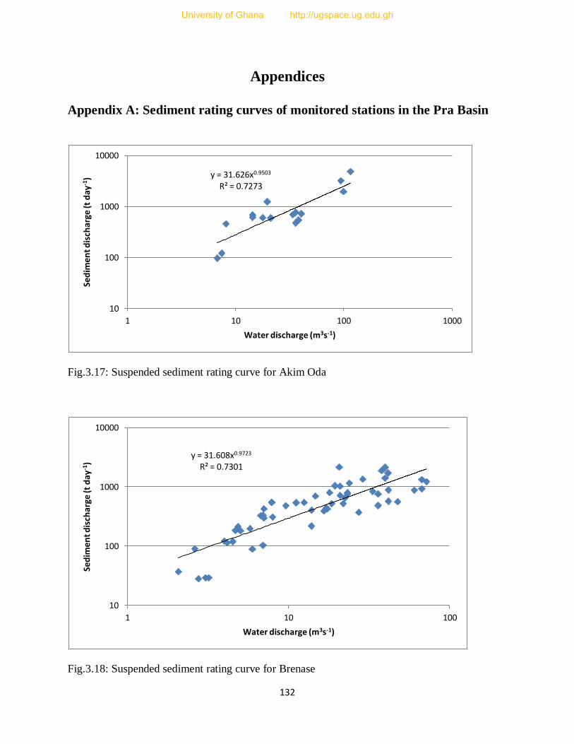
132

Appendices

Appendix A: Sediment rating curves of monitored stations in the Pra Basin

Fig.3.17: Suspended sediment rating curve for Akim Oda

Fig.3.18: Suspended sediment rating curve for Brenase

y = 31.626x0.9503 R² = 0.7273

10

100

1000

10000

1 10 100 1000

Sed

ime

nt d

isch

arge

(t d

ay-1

)

Water discharge (m3s-1)

y = 31.608x0.9723 R² = 0.7301

10

100

1000

10000

1 10 100

Sed

imen

t dis

char

ge (t

day

-1)



133

Fig.3.19: Suspended sediment rating curve for Anwiankwanta

Fig.3.20: Suspended sediment rating curve for Adiembra

y = 13.676x1.1527 R² = 0.8607

10

100

1000

10000

1 10 100

Sed

ime

nt d

isch

arge

(t d

ay-1

)


y = 10.914x0.9737 R² = 0.8614

1

10

100

1000

10000

1 10 100 1000

Sed

imen

t dis

char

ge (t

day

-1)



134

Fig.3.21: Suspended sediment rating curve for Twifo Praso

Fig.3.22: Suspended sediment rating curve for Assin Praso

y = 100.38x0.897 R² = 0.983

10

100

1000

10000

100000

0.1 1 10 100 1000

Sed

ime

nt d

isch

arge

(t d

ay-1

)


y = 14.638x1.1156 R² = 0.924

10

100

1000

10000

1 10 100 1000

Sed

imen

t dis

char

ge (t

day

-1)



135

Fig.3.23: Suspended sediment rating curve for Sekyere Heman

Hypothesis Testing

Model1:

Yield ~ AREA

Df Sum of Sq RSS AIC F value Pr(>F)

<none> 1.1710e+13 201.02

AREA 1 3.4333e+13 4.6043e+13 208.60 14.659 0.01226 *

Signif. codes: 0 ‘***’ 0.001 ‘**’ 0.01 ‘*’ 0.05 ‘.’ 0.1 ‘ ’ 1

> summary(model1)

Call:

lm(formula = Yield ~ AREA, data = Sedimentyield_BasinArea)

Residuals:

1 2 3 4 5 6 7

491506 65663 240257 345277 -1435865 -1996171 2289334

y = 429.48x0.6666 R² = 0.6628

10000

100000

100 1000 10000

Sed

ime

nt d

isch

arge

(t d

ay-1

)



136

Coefficients:

Estimate Std. Error t value Pr(>|t|)

(Intercept) -762798.44 839798.72 -0.908 0.4054

AREA 262.01 68.43 3.829 0.0123 *

Signif. codes: 0 ‘***’ 0.001 ‘**’ 0.01 ‘*’ 0.05 ‘.’ 0.1 ‘ ’ 1

Residual standard error: 1530000 on 5 degrees of freedom

Multiple R-squared: 0.7457, Adjusted R-squared: 0.6948

F-statistic: 14.66 on 1 and 5 DF, p-value: 0.01226

Model2:

>cor(Sedimentyield_BasinArea, method = "kendall")

No. Yield AREA SSY

No. 1.0000000 0.8095238 0.8095238 0.4285714

Yield 0.8095238 1.0000000 0.8095238 0.6190476

AREA 0.8095238 0.8095238 1.0000000 0.4285714

SSY 0.4285714 0.6190476 0.4285714 1.0000000

Model3:

> cor(Sedimentyield_BasinArea, method = "spearm")

No. Yield AREA SSY

No. 1.0000000 0.8928571 0.8928571 0.5714286

Yield 0.8928571 1.0000000 0.9285714 0.7500000

AREA 0.8928571 0.9285714 1.0000000 0.5357143

SSY 0.5714286 0.7500000 0.5357143 1.0000000


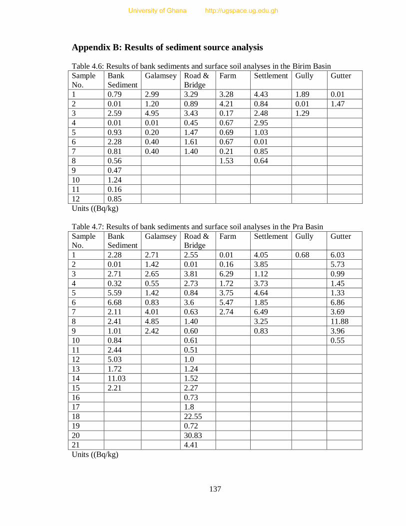
137

Appendix B: Results of sediment source analysis

Table 4.6: Results of bank sediments and surface soil analyses in the Birim Basin

Sample

No.

Bank

Sediment

Galamsey

Road &

Bridge

Farm

Settlement

Gully

Gutter

1 0.79 2.99 3.29 3.28 4.43 1.89 0.01

2 0.01 1.20 0.89 4.21 0.84 0.01 1.47

3 2.59 4.95 3.43 0.17 2.48 1.29

4 0.01 0.01 0.45 0.67 2.95

5 0.93 0.20 1.47 0.69 1.03

6 2.28 0.40 1.61 0.67 0.01

7 0.81 0.40 1.40 0.21 0.85

8 0.56 1.53 0.64

9 0.47

10 1.24

11 0.16

12 0.85

Units ((Bq/kg)

Table 4.7: Results of bank sediments and surface soil analyses in the Pra Basin

Sample

No.

Bank

Sediment

Galamsey

Road &

Bridge

Farm

Settlement

Gully

Gutter

1 2.28 2.71 2.55 0.01 4.05 0.68 6.03

2 0.01 1.42 0.01 0.16 3.85 5.73

3 2.71 2.65 3.81 6.29 1.12 0.99

4 0.32 0.55 2.73 1.72 3.73 1.45

5 5.59 1.42 0.84 3.75 4.64 1.33

6 6.68 0.83 3.6 5.47 1.85 6.86

7 2.11 4.01 0.63 2.74 6.49 3.69

8 2.41 4.85 1.40 3.25 11.88

9 1.01 2.42 0.60 0.83 3.96

10 0.84 0.61 0.55

11 2.44 0.51

12 5.03 1.0

13 1.72 1.24

14 11.03 1.52

15 2.21 2.27

16 0.73

17 1.8

18 22.55

19 0.72

20 30.83

21 4.41

Units ((Bq/kg)


138

Table 4.8: Results of bank sediments and surface soil analyses in the Oda Basin

Sample

No.

Bank

Sediment

Galamsey

Road &

Bridge

Settlement

Gully

Gutter

1 0.01 0.01 0.05 0.01 1.36 5.7

2 1.24 0.01 3.05 0.01 3.32 0.2

3 1.35 0.01 1.07 3.67

4 1.99 0.91 2.95 2.26

5 2.68 1.25

6 2.27

7 8.27

8 2.27

9 1.10

10 1.69

11 2.54

12 0.03

Units ((Bq/kg)

Table 4.9: Results of bank sediments and surface soil analyses in the Ofin Basin Basin

Sample

No.

Bank

Sediment

Galamsey

Road &

Bridge

Farm

Settlement

Gully

Gutter

1 3.05 2.81 4.74 1.36 3.57 0.01 0.01

2 0.01 1.69 3.37 0.89 2.1 1.69 0.01

3 0.56 0.01 1.53

4 0.01 0.01

5 1.64 4.08

6 1.11 1.56

7 0.58 0.48

8 1.09 3.48

Units ((Bq/kg)

Hypothesis Testing

Model1:

Stream_Sediment ~ Surface_soil + Bank_sediment


<none> 0.00156 -25.3984

Surface_soil 1 0.00002 0.00158 -27.3412 0.0144 0.92395

Bank_sediment 1 0.43321 0.43477 -4.8769 277.7630 0.03815 *

---

Signif. codes: 0 ‘***’ 0.001 ‘**’ 0.01 ‘*’ 0.05 ‘.’ 0.1 ‘ ’ 1

>

> summary(model1)


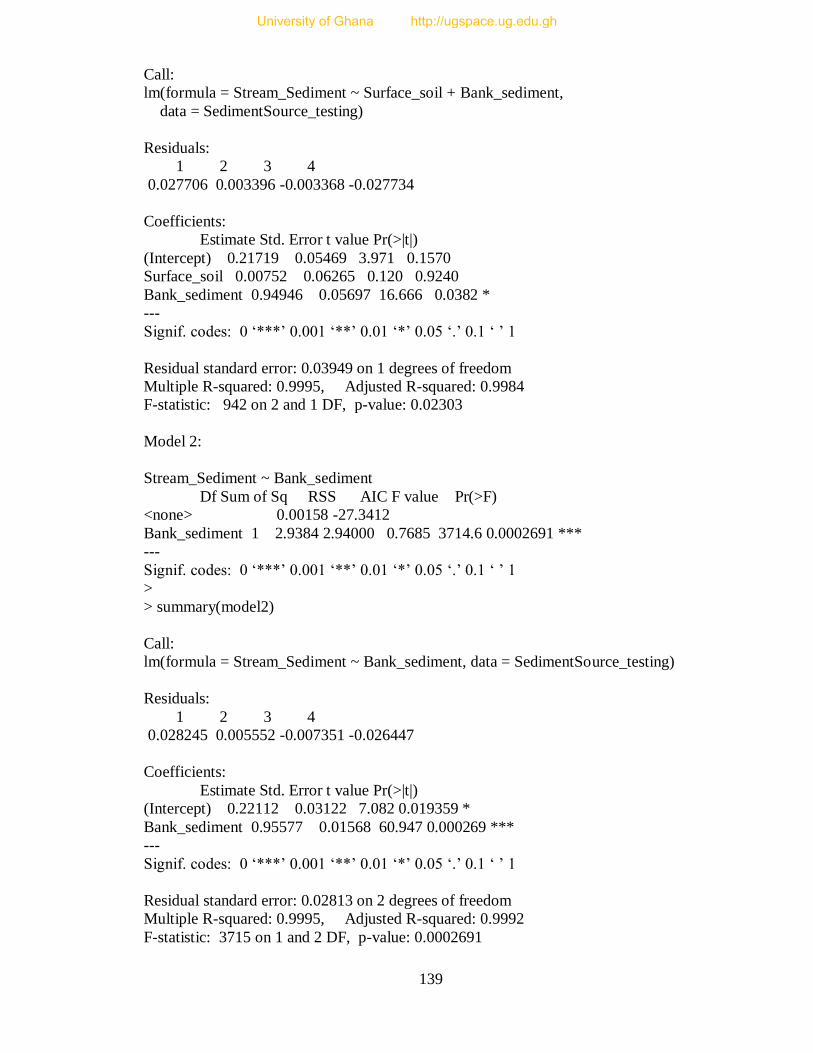
139

Call:

lm(formula = Stream_Sediment ~ Surface_soil + Bank_sediment,

data = SedimentSource_testing)

Residuals:

1 2 3 4

0.027706 0.003396 -0.003368 -0.027734

Coefficients:


(Intercept) 0.21719 0.05469 3.971 0.1570

Surface_soil 0.00752 0.06265 0.120 0.9240

Bank_sediment 0.94946 0.05697 16.666 0.0382 *

---

Signif. codes: 0 ‘***’ 0.001 ‘**’ 0.01 ‘*’ 0.05 ‘.’ 0.1 ‘ ’ 1

Residual standard error: 0.03949 on 1 degrees of freedom


F-statistic: 942 on 2 and 1 DF, p-value: 0.02303

Model 2:

Stream_Sediment ~ Bank_sediment


<none> 0.00158 -27.3412

Bank_sediment 1 2.9384 2.94000 0.7685 3714.6 0.0002691 ***

---

Signif. codes: 0 ‘***’ 0.001 ‘**’ 0.01 ‘*’ 0.05 ‘.’ 0.1 ‘ ’ 1

>

> summary(model2)

Call:

lm(formula = Stream_Sediment ~ Bank_sediment, data = SedimentSource_testing)

Residuals:

1 2 3 4

0.028245 0.005552 -0.007351 -0.026447

Coefficients:


(Intercept) 0.22112 0.03122 7.082 0.019359 *

Bank_sediment 0.95577 0.01568 60.947 0.000269 ***

---

Signif. codes: 0 ‘***’ 0.001 ‘**’ 0.01 ‘*’ 0.05 ‘.’ 0.1 ‘ ’ 1



F-statistic: 3715 on 1 and 2 DF, p-value: 0.0002691


140

Model3:

Stream_Sediment ~ Surface_soil


<none> 0.43477 -4.8769

Surface_soil 1 2.5052 2.94000 0.7685 11.524 0.0769 .

---

Signif. codes: 0 ‘***’ 0.001 ‘**’ 0.01 ‘*’ 0.05 ‘.’ 0.1 ‘ ’ 1

>

> summary(model3)

Call:

lm(formula = Stream_Sediment ~ Surface_soil, data = SedimentSource_testing)

Residuals:

1 2 3 4

-0.16729 -0.08666 0.55536 -0.30141

Coefficients:


(Intercept) -0.03327 0.62081 -0.054 0.9621

Surface_soil 0.97057 0.28590 3.395 0.0769 .

---

Signif. codes: 0 ‘***’ 0.001 ‘**’ 0.01 ‘*’ 0.05 ‘.’ 0.1 ‘ ’ 1



F-statistic: 11.52 on 1 and 2 DF, p-value: 0.0769


141

Appendix C: Data sheet of erosion pin measurements and grain size analysis

Table 5.7: Measurements of bank erosion and deposition at Akim Oda

Date 4th September 2012 6

th March 2013

Length of exposure of pins/cm (“+” erosion

and “-“ Deposition)




Location

Pin 1 Pin 2 Pin 3 Pin 4 Pin 1 Pin 2 Pin 3 Pin 4

Birim Akim

Oda

Left Top 1 1 Bank

failure

Bank

failure

11 3 17 Bank

failure

Left Middle 1.3 15 buried buried 3 5 4.5 buried

Left Bottom 10.5 8 buried buried buried buried buried buried

Table 5.8: Measurements of bank erosion and deposition at Amuanda Praso


th March 2013

Length of exposure of pins/cm (“+”

erosion and “-“ Deposition)




Location

Pin 1 Pin 2 Pin 3 Pin 1 Pin 2 Pin 3

Pra Amuanda Right Top -1 0.7 buried buried buried buried

Right Middle -2 1 buried buried buried 2.5

Right Bottom -0.5 buried buried 6 6 5.5

Left Top 3 -2 1.5 2.8 1.5 1.5

Left Middle buried buried buried 3 1 5

Left Bottom 1 submerged 1.4 4.5 4 5


142

Table 5.9: Measurements of bank erosion and deposition at Praso

Date 17th August, 2012 5

th March, 2013






Location

Pin 1 Pin 2 Pin 3 Pin 1 Pin 2 Pin 3

Pra Praso Right Top -3.0 -2.5 buried 0 0.5 buried

Right Bottom -4.0 buried buried buried buried buried

Left Top 1.0 1.0 1.4 0.2 1.0 1.5

Left Bottom 1.2 1.5 1.0 1.0 1.5 1.7

Table 5.10: Measurements of bank erosion and deposition at Anyinam

Date 5th March 2013




Location

Pin 1 Pin 2 Pin 3 Pin 4 Pin 5

Birim Anyinam Left Top 0.0 0.0 0.5 3 1

Left Bottom 1.0 0.5 2.0 1.5 3.7

Right Top Deposition of sediments of depth between 2 – 17cm

Right Bottom Deposition of sediments of depth between 20 – 65cm

NB: Due to high flows, measurements were only possible once in the year


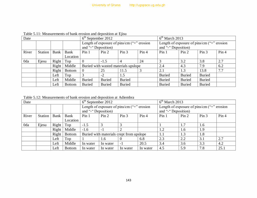
143

Table 5.11: Measurements of bank erosion and deposition at Ejisu


th March 2013






Location


0da Ejesu Right Top 0 -1.5 4 24 3 3.2 3.8 2.7

Right Middle Buried with wasted materials upslope 2.4 4.3 7.9 6.2

Right Bottom 0 25 11.5 3 2.1 1.3 13.8 7.7

Left Top 3 -2 1.5 Buried Buried Buried

Left Middle Buried Buried Buried Buried Buried Buried

Left Bottom Buried Buried Buried Buried Buried Buried

Table 5.12: Measurements of bank erosion and deposition at Adiembra


th March 2013






Location


0da Ejesu Right Top -1.5 3 3 1 1.7 1.6

Right Middle -1.6 -1 2 1.2 1.6 1.9

Right Bottom Buried with materials crept from upslope 1.1 1.3 1.8

Left Top 1 1.6 0 6.8 2.3 2.2 3.1 2.7

Left Middle In water In water -1 20.5 3.4 3.6 3.3 4.2

Left Bottom In water In water In water In water 4.5 5.9 7.8 25.1


144

Table 5.13: Grain size analyses of bank sediments at Anyinam and Ejisu

Anyinam Ejisu

Sieve

Opening(mm)

Weight

on

Sieve/gm

%

Remaining

on sieve

Cumulative

%

remaining

on sieve

Cumulative

% passing

Weight on

Sieve/gm

%

Remaining

on sieve

Cumulative

%

remaining

on sieve

Cumulative

% passing

0.002 35.3 6.8 100 6.8 52.6 3.8 100 3.6

0.05 22.9 4.4 93.2 11.2 127 8.6 96.4 12.2

0.1 65.6 12.6 88.8 23.8 526.6 35.8 87.8 47.9

0.25 62.4 12.0 76.3 35.72 285.4 19.4 52.1 67.3

0.5 87.1 16.7 64.3 52.4 133.9 9.1 32.7 76.4

1 111.3 21.4 47.6 73.8 129 8.8 23.6 85.2

2 41.8 8.0 26.2 81.8 44.6 3.0 14.8 88.2

2.5 94.9 18.2 18.2 100 173.9 11.8 11.8 100

Total 521.3 1473

Table 5.14: Grain size analyses of bank sediments at Akim Oda

Sample A Sample B

Sieve

Opening(mm)

Weight

on

Sieve/gm

%

Remaining

on sieve

Cumulative

%

remaining

on sieve

Cumulative

% passing

Weight

on

Sieve/gm

%

Remaining

on sieve

Cumulative

%

remaining

on sieve

Cumulative

% passing

0.002 79.2 7.1 100 7.1 38.8 2.3 100 2.3

0.05 171.8 15.5 92. 9 22.6 92.9 5.4 97.7 7.7

0.1 309.6 27.9 77.4 50.5 152.1 8.9 92.3 16.6

0.25 89.1 8.0 49.5 58.6 56.8 3.3 83.4 20.0

0.5 119.9 10.8 41.5 69.4 58.5 3.4 80.1 23.4

1 135.1 12.2 30.7 81.5 84.3 4.9 76.6 28.3

2 51.5 4.6 18.5 86.2 41.2 2.4 71.7 30.7

2.5 153.5 13.8 13.8 100 1182.4 69.3 69.3 100

Total 1109.7 1707


145

Table 5.15: Grain size analyses of bank sediments at Adiembra

Sample A (left bank) Sample B (right bank)

Sieve

Opening(mm)

Weight

on

Sieve/gm

%

Remaining

on sieve

Cumulative

%

remaining

on sieve

Cumulative

% passing

Weight on

Sieve/gm

%

Remaining

on sieve

Cumulative

%

remaining

on sieve

Cumulative

% passing

0.002 0.002 67.80 6.14 100 0.002 50.5 4.1 100

0.05 0.05 150.90 13.66 93.86 0.05 179.5 14.7 95.9

0.1 0.1 475.20 43.01 80.21 0.1 750.8 61.4 81.2

0.25 0.25 67.90 6.15 37.20 0.25 83.7 6.9 19.8

0.5 0.5 61.20 5.54 31.05 0.5 59.5 4.9 12.9

1 1.0 88.90 8.05 25.51 1 56.4 4.6 8.1

2 2.0 48.60 4.40 17.47 2 15.1 1.2 3.5

2.5 2.5 144.40 13.07 13.07 2.5 27.1 2.2 2.2

Total 1104.9 1222.6


sediment yield and bank erosion assessment of pra river ... yield... · this thesis entitled...

Documents