rigid body dynamics - computing sciencetorsten/teaching/cmpt466/lecturenotes/pdf/09_rigid… ·...
TRANSCRIPT

© Möller/Parent/Machiraju
Rigid Body Dynamics
CMPT 466
Computer Animation
Torsten Möller
© Möller/Parent/Machiraju
Advanced Algorithms
• Hierarchical Kinematic Modeling
– Forward Kinematics
– Inverse Kinematics
• Rigid Body Constraints
– Basic Particle Forces
– Collision
• Controlling Groups of Objects
– particle systems
– flocking behaviour
© Möller/Parent/Machiraju
Reading
• Chapter 4 of Parents book
• Foley, van Dam, etc.; Angel; Watt;
Glassner; Hill; Baker + Hearns
© Möller/Parent/Machiraju
Rigid Body Dynamics
• Keyframing can be tedious - especially to
get ‘realism’
• Simulate physics by
– programming equations of motions
– setting initial conditions
• Animator gives up control
• Animator gets ‘realistic’ motion
automatically.

© Möller/Parent/Machiraju
Simulation Update Cycle
Object properties
Position, orientation
Linear and angular velocity
Linear and angular momentum
mass
Calculate forces
Calculate accelerations
Using mass, momenta
Update object properties
© Möller/Parent/Machiraju
Particle Under Forces
• Forces
– Gravity
– Wind
– Springs
– Collision avoidance
– Soft constraints
• Calculate acceleration due to forces
• Calculate update to object velocity &position
© Möller/Parent/Machiraju
Forces - Basic Physics
• Friction - static and kinematic
• Gravity
• Viscosity
• Springs (Hooke’s law)
• Damping
© Möller/Parent/Machiraju
F
Fs
!
Fs
= usFN
Friction
• Supporting object
• Resting contact
• Normal force
• Static friction
© Möller/Parent/Machiraju
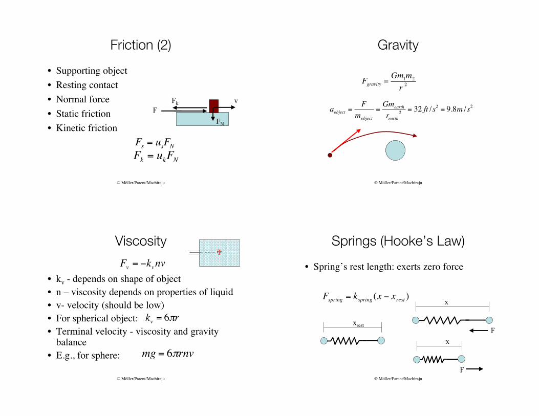
!
Fs
= usFN
!
Fk
= ukFN
FN
v
F
Fk
Friction (2)
• Supporting object
• Resting contact
• Normal force
• Static friction
• Kinetic friction
© Möller/Parent/Machiraju
!
Fgravity =Gm
1m2
r2
!
aobject =F
mobject
=Gmearth
rearth2
= 32 ft /s2
= 9.8m /s2
Gravity
© Möller/Parent/Machiraju
• kv - depends on shape of object
• n – viscosity depends on properties of liquid
• v- velocity (should be low)
• For spherical object:
• Terminal velocity - viscosity and gravitybalance
• E.g., for sphere:
!
Fv
= "kvnv
!
kv
= 6"r
!
mg = 6"rnv
Viscosity
© Möller/Parent/Machiraju
!
Fspring = kspring (x " xrest )
xrest
x
x
F
F
Springs (Hooke’s Law)
• Spring’s rest length: exerts zero force
© Möller/Parent/Machiraju
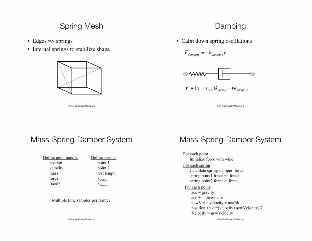
Spring Mesh
• Edges => springs
• Internal springs to stabilize shape
© Möller/Parent/Machiraju
!
Fdamping = "kdampingv
!
F = (x " xrest )kspring " vkdamping
Damping
• Calm down spring oscillations
© Möller/Parent/Machiraju
Define point masses
postion
velocity
mass
force
fixed?
Define springs
point 1
point 2
rest length
kspring
kdamper
Multiple time samples per frame?
Mass-Spring-Damper System
© Möller/Parent/Machiraju
For each point
Initialize force with wind
For each spring
Calculate spring-damper force
spring.point1.force += force
spring.point2.force -= force
For each point
acc = gravity
acc += force/mass
newVel = velocity + acc*dt
position += dt*(velocity+newVelocity)/2
Velocity = newVelocity
Mass-Spring-Damper System

© Möller/Parent/Machiraju
Examples
• 1, 4, 16 time samples per frame
© Möller/Parent/Machiraju
Examples (2)
• Multiple connectivity; fixing a node adding
gravity and wind
© Möller/Parent/Machiraju
Examples (3)
• Adding damping; making a flag
• Use controlled random numbers to add
interest
© Möller/Parent/Machiraju
Randomize
• Controlled randomness adds more interest
– To initial values (positions, velocities)
– To force fields (wind direction, wind speed)
– To spring constants, masses
– To joint angles
• Proximal joints: lower amplitude
• Distal joints: higher amplitude
• Coordinate frequency and phase
© Möller/Parent/Machiraju
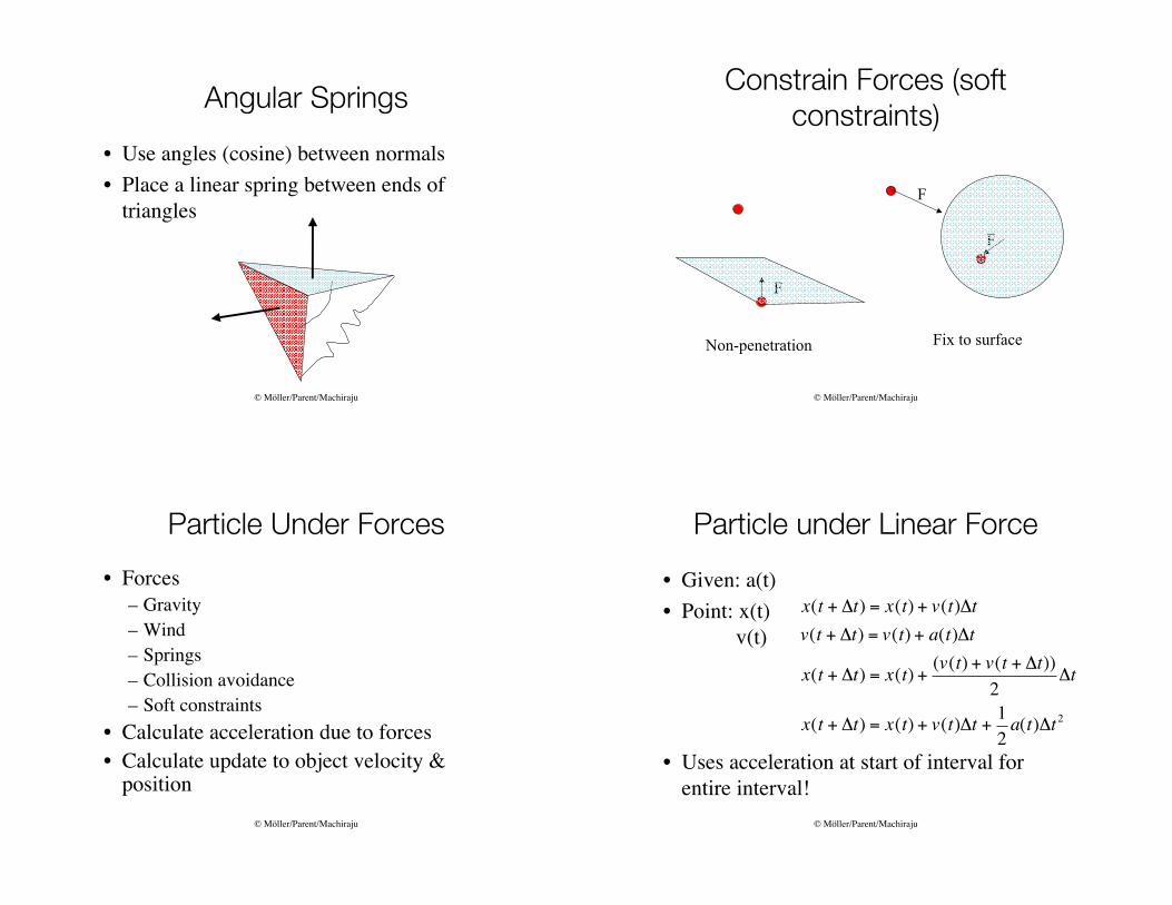
Angular Springs
• Use angles (cosine) between normals
• Place a linear spring between ends of
triangles
© Möller/Parent/Machiraju
Constrain Forces (soft
constraints)
F
F
F
Non-penetration Fix to surface
© Möller/Parent/Machiraju
Particle Under Forces
• Forces
– Gravity
– Wind
– Springs
– Collision avoidance
– Soft constraints
• Calculate acceleration due to forces
• Calculate update to object velocity &position
© Möller/Parent/Machiraju!
x(t + "t) = x(t) + v(t)"t
v(t + "t) = v(t) + a(t)"t
x(t + "t) = x(t) +(v(t) + v(t + "t))
2"t
x(t + "t) = x(t) + v(t)"t +1
2a(t)"t 2
Particle under Linear Force
• Given: a(t)
• Point: x(t)
v(t)
• Uses acceleration at start of interval for
entire interval!
© Möller/Parent/Machiraju
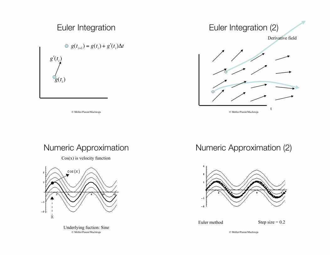
Euler Integration
!
g(ti+1) = g(ti) + " g (ti)#t
!
" g (ti)
!
g(ti)
© Möller/Parent/Machiraju
Euler Integration (2)
t
Derivative field
© Möller/Parent/Machiraju
Numeric Approximation
Underlying fuction: Sine
Cos(x) is velocity function
© Möller/Parent/Machiraju
Numeric Approximation (2)
Step size = 0.2Euler method
© Möller/Parent/Machiraju
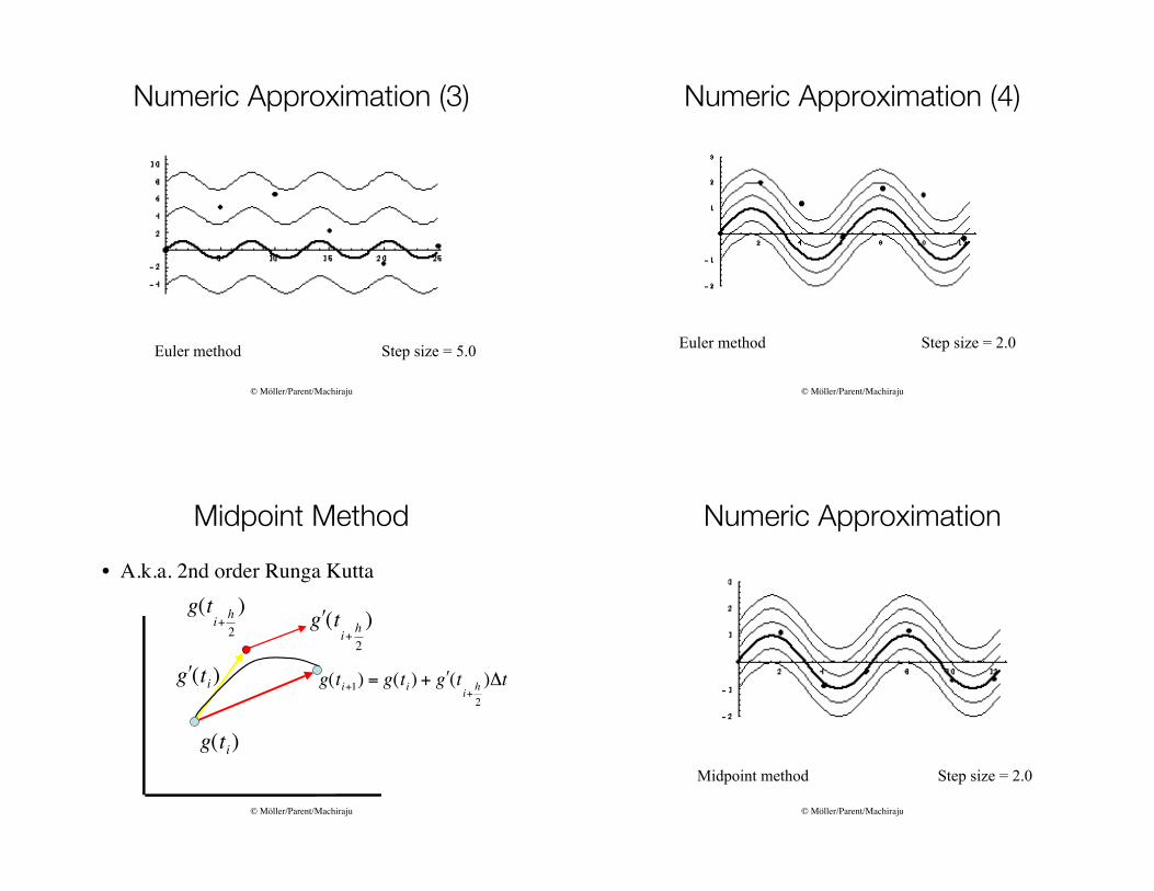
Numeric Approximation (3)
Step size = 5.0Euler method
© Möller/Parent/Machiraju
Numeric Approximation (4)
Euler method Step size = 2.0
© Möller/Parent/Machiraju
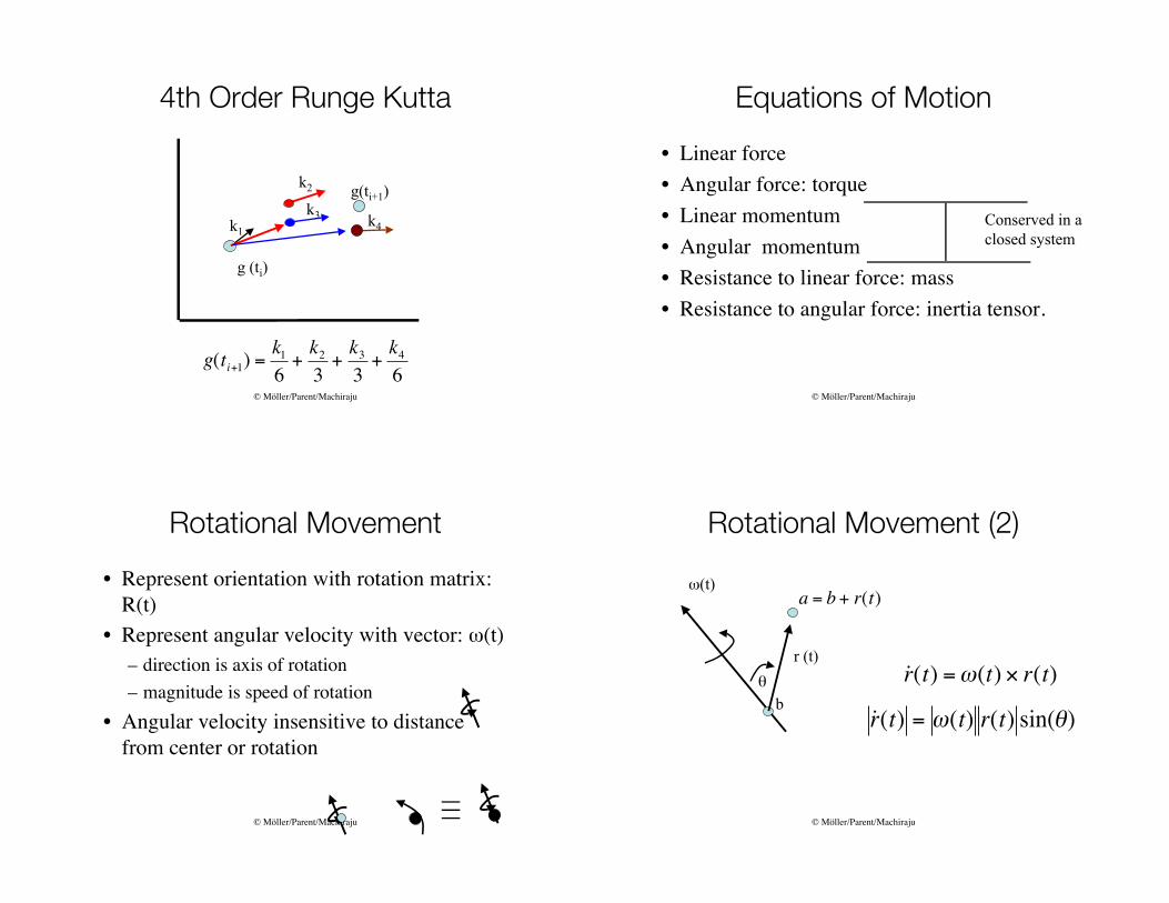
Midpoint Method
• A.k.a. 2nd order Runga Kutta
!
g(ti+h
2
)
!
" g (ti)
!
" g (ti+
h
2
)
!
g(ti)
!
g(ti+1) = g(ti) + " g (ti+
h
2
)#t
© Möller/Parent/Machiraju
Numeric Approximation
Midpoint method Step size = 2.0
© Möller/Parent/Machiraju
4th Order Runge Kutta
g (ti)
!
g(ti+1) =k1
6+k2
3+k3
3+k4
6
g(ti+1)
k1
k2
k3 k4
© Möller/Parent/Machiraju
Conserved in a
closed system
Equations of Motion
• Linear force
• Angular force: torque
• Linear momentum
• Angular momentum
• Resistance to linear force: mass
• Resistance to angular force: inertia tensor.
© Möller/Parent/Machiraju
Rotational Movement
• Represent orientation with rotation matrix:
R(t)
• Represent angular velocity with vector: !(t)
– direction is axis of rotation
– magnitude is speed of rotation
• Angular velocity insensitive to distance
from center or rotation
© Möller/Parent/Machiraju
Rotational Movement (2)
b
r (t)
"
!(t)
!
˙ r (t) = "(t) r(t) sin(#)
!
˙ r (t) ="(t) # r(t)!
a = b + r(t)

© Möller/Parent/Machiraju
Rotational Movement (3)
!
R(t) = R1(t) R
2(t) R
3(t)[ ]
!
˙ R (t) = "(t) # R1(t) "(t) # R
2(t) "(t) # R
3(t)[ ]
( ) BA
B
B
B
AA
AA
AA
BABA
BABA
BABA
BA
z
y
x
xy
xz
yz
xyyx
zxxz
yzzy
*
0
0
0
=
!!!
"
#
$$$
%
&
!!!
"
#
$$$
%
&
'
'
'
=
!!!
"
#
$$$
%
&
('(
('('
('(
=)
Define the following for notational convenience:
It is the dual notation !
© Möller/Parent/Machiraju
!
˙ R (t) ="(t)*R(t)
q(t) = R(t)q + x(t)
˙ q (t) ="(t) # (R(t)q) + v(t)
˙ q (t) ="(t) # (q(t) $ x(t)) + v(t)
Rotational Movement (4)
• q is on object and x(t), R(t) is position,
orientation of object
© Möller/Parent/Machiraju
• Points are often used in CG for masses and
objects
• Integration of differential mass times
position in object
!
M = mi"
!
x(t) =miqi(t)"M
Center of Mass
© Möller/Parent/Machiraju
Force and Torque
!
F = ma
a = F /m
F(t) = f i(t)"# i(t) = (q(t) $ x(t)) % f i(t)
#(t) = # i(t)"F
F
© Möller/Parent/Machiraju
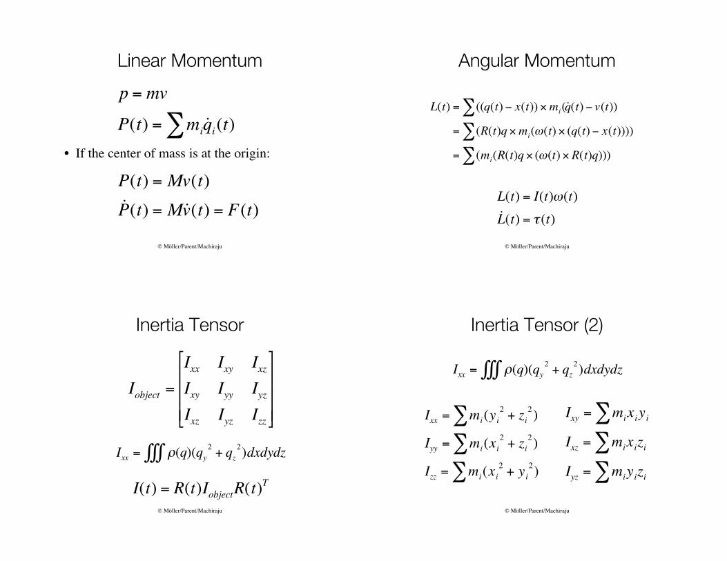
Linear Momentum
!
p = mv
P(t) = mi˙ q i(t)"
• If the center of mass is at the origin:
!
P(t) = Mv(t)
˙ P (t) = M ˙ v (t) = F(t)
© Möller/Parent/Machiraju
Angular Momentum
!
L(t) = ((q(t) " x(t)) #mi($ ˙ q (t) " v(t))
= (R(t)q #mi(%(t) # (q(t) " x(t))))$
= (mi(R(t)q # (%(t) # R(t)q)))$
!
L(t) = I(t)"(t)
˙ L (t) = # (t)
© Möller/Parent/Machiraju
Inertia Tensor
!
Iobject =
Ixx Ixy Ixz
Ixy Iyy Iyz
Ixz Iyz Izz
"
#
$ $ $
%
&
' ' '
!
I(t) = R(t)IobjectR(t)T
!
Ixx = "(q)(qy2### + qz
2)dxdydz
© Möller/Parent/Machiraju
Inertia Tensor (2)
!
Ixx = "(q)(qy2### + qz
2)dxdydz
!
Ixx = mi(yi2
+ zi2)"
Iyy = mi(xi2
+ zi2)"
Izz = mi(xi2
+ yi2)"
!
Ixy = mixiyi"
Ixz = mixizi"
Iyz = miyizi"
© Möller/Parent/Machiraju
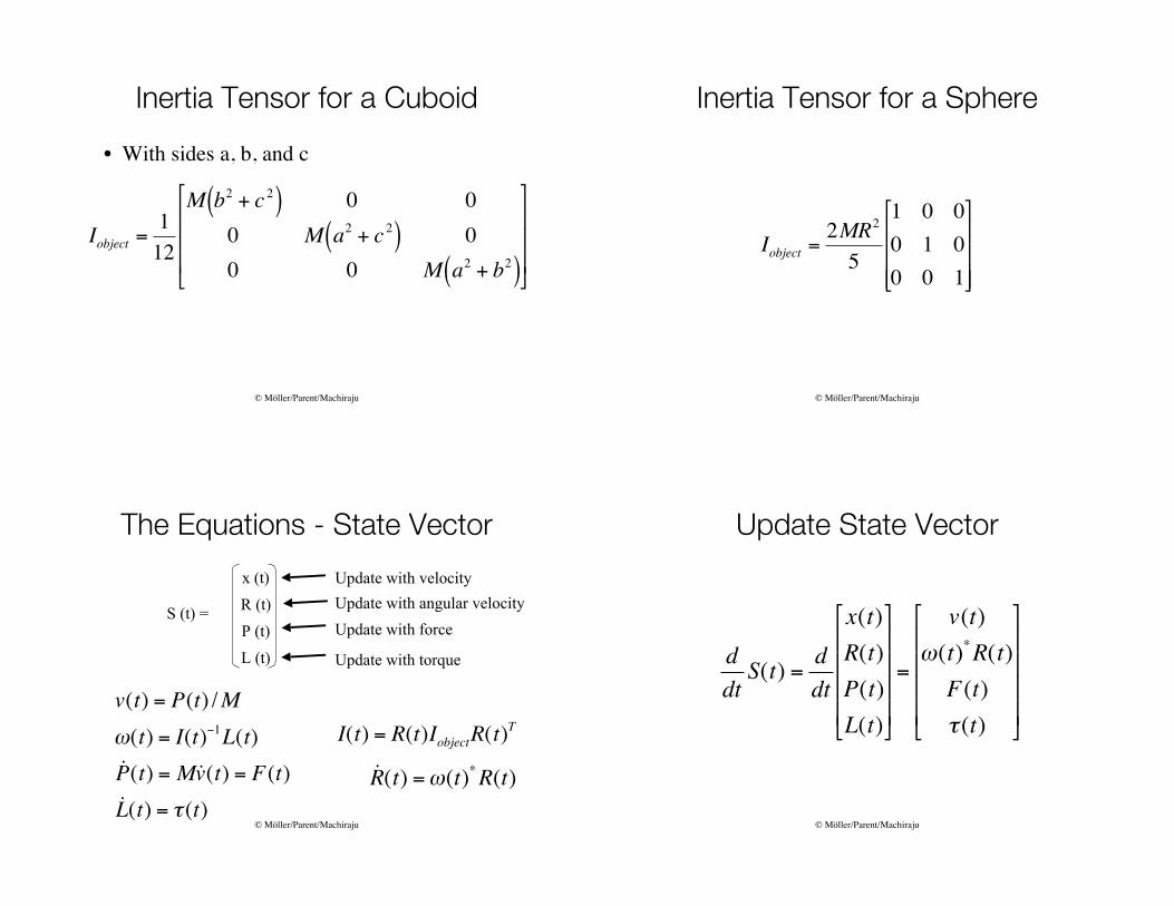
Inertia Tensor for a Cuboid
!
Iobject =1
12
M b2 + c 2( ) 0 0
0 M a2 + c 2( ) 0
0 0 M a2 + b2( )
"
#
$ $ $
%
&
' ' '
• With sides a, b, and c
© Möller/Parent/Machiraju
Inertia Tensor for a Sphere
!
Iobject =2MR
2
5
1 0 0
0 1 0
0 0 1
"
#
$ $ $
%
&
' ' '
© Möller/Parent/Machiraju
The Equations - State Vector
S (t) =
x (t)
R (t)
P (t)
L (t)
Update with velocity
Update with angular velocity
Update with force
Update with torque
!
v(t) = P(t) / M
"(t) = I(t)#1
L(t)
˙ P (t) = M ˙ v (t) = F(t)
˙ L (t) = $ (t)
!
I(t) = R(t)IobjectR(t)T
!
˙ R (t) ="(t)*R(t)
© Möller/Parent/Machiraju
Update State Vector
!
d
dtS(t) =
d
dt
x(t)
R(t)
P(t)
L(t)
"
#
$ $ $ $
%
&
' ' ' '
=
v(t)
((t)*R(t)
F(t)
) (t)
"
#
$ $ $ $
%
&
' ' ' '
© Möller/Parent/Machiraju
Update Orientation
• ! (t) * R(t) and renormalize
• Extract axis-angle from ! (t) and rotate
columns of R(t)
• Use quaternions
© Möller/Parent/Machiraju
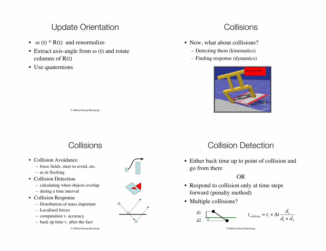
Baraff 1991
Collisions
• Now, what about collisions?
– Detecting them (kinematics)
– Finding response (dynamics)
© Möller/Parent/Machiraju
Collisions
• Collision Avoidance
– force fields, steer to avoid, etc.
– as in flocking
• Collision Detection
– calculating when objects overlap
– during a time interval
• Collision Response
– Distribution of mass important
– Localized forces
– computation v. accuracy
– back up time v. after-the-fact
© Möller/Parent/Machiraju
d1
d2
!
tcollision
= ti+ "t
d1
d1
+ d2
Collision Detection
• Either back time up to point of collision and
go from there
OR
• Respond to collision only at time steps
forward (penalty method)
• Multiple collisions?
© Möller/Parent/Machiraju
Collision Resp. Strategies
• Strictly kinematical response
– quick and easy
– good visual results for (spherical) particles
• Penalty method
– used when no backing up in time is enforced
– easy to use, however, forces can be unnatural
• Impulse forces
– Usually used when time is backed up
© Möller/Parent/Machiraju
!
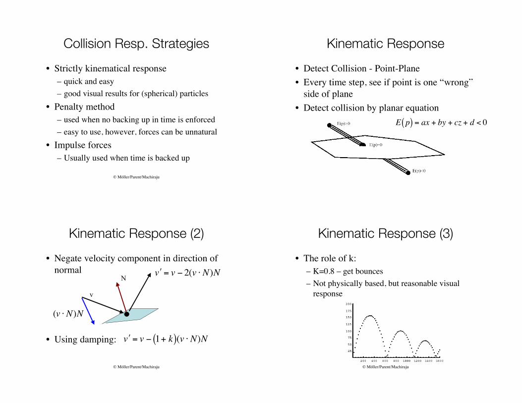
E p( ) = ax + by + cz + d < 0
Kinematic Response
• Detect Collision - Point-Plane
• Every time step, see if point is one “wrong”
side of plane
• Detect collision by planar equation
© Möller/Parent/Machiraju
Kinematic Response (2)
• Negate velocity component in direction of
normal
• Using damping:
v
N
!
" v = v # 2(v $ N)N
!
(v " N)N
!
" v = v # 1+ k( )(v $ N)N
© Möller/Parent/Machiraju
Kinematic Response (3)
• The role of k:
– K=0.8 – get bounces
– Not physically based, but reasonable visual
response

© Möller/Parent/Machiraju
Penalty Method
• Associate closest point of object with spring
• Penalize when interpenetration occurs
• Spring force F = k*d
• Apply –F to point
• Compute acceleration and effect velocity along
normal
d© Möller/Parent/Machiraju
Testing Planar Polyhedra
• Point inside a convex/concave polyhedron
test
• Edge-plane intersection
• Temporal aliasing can occur
© Möller/Parent/Machiraju
Swept Volumes
• Compute motion of one relative to other
• Compute swept volume
• Determine if other object intersects swept
volume
• Tractable only for simple motion
© Möller/Parent/Machiraju
After collision is detected
• Consider applying a force to both bodies
– nature “simulates” collisions like this
– Interpenetrating objects will remain so for at
least one more time step
• Cannot instantaneously change velocity
• Forces need time to be integrated to accelerations
and velocities
© Möller/Parent/Machiraju
After collision is detected
• Still, we need instantaneous change in
velocity => Impulse
– A hack for impenetrable bodies exist
– Generalization of subtle surface properties
– Simulates a large force for a small time step
– Will change velocity like we need
© Möller/Parent/Machiraju
Calculating impulse
• Duration of impulse is “no time”
– Actually a small amount of time
– Other forces ignored during this period
• No friction too !
© Möller/Parent/Machiraju
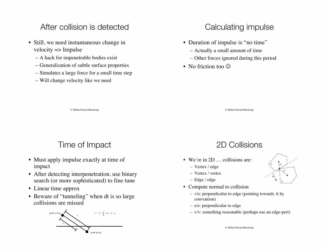
Time of Impact
• Must apply impulse exactly at time ofimpact
• After detecting interpenetration, use binarysearch (or more sophisticated) to fine tune
• Linear time approx
• Beware of “tunneling” when dt is so largecollisions are missed
© Möller/Parent/Machiraju
2D Collisions
• We’re in 2D … collisions are:
– Vertex / edge
– Vertex / vertex
– Edge / edge
• Compute normal to collision
– v/e: perpendicular to edge (pointing towards A by
convention)
– e/e: perpendicular to edge
– v/v: something reasonable (perhaps use an edge-pert)
© Möller/Parent/Machiraju
More Remarks
• Edge/edge collisions are modeled as
point/point in this system
• Only two colliding bodies at a time
• 3D is harder because of variety of collision
types
© Möller/Parent/Machiraju
!
J = F"t = Ma"t = M"v = "(Mv) = "P
!
J = jN
Impulse Force of Collision
• Compute change in momentum
• Impulse is in the direction of the normal:
© Möller/Parent/Machiraju
Equal and
opposite
Calculating an impulse
• Solve for one number, j
– Apply j in direction of N to A
– Apply j in direction of –N to B
© Möller/Parent/Machiraju
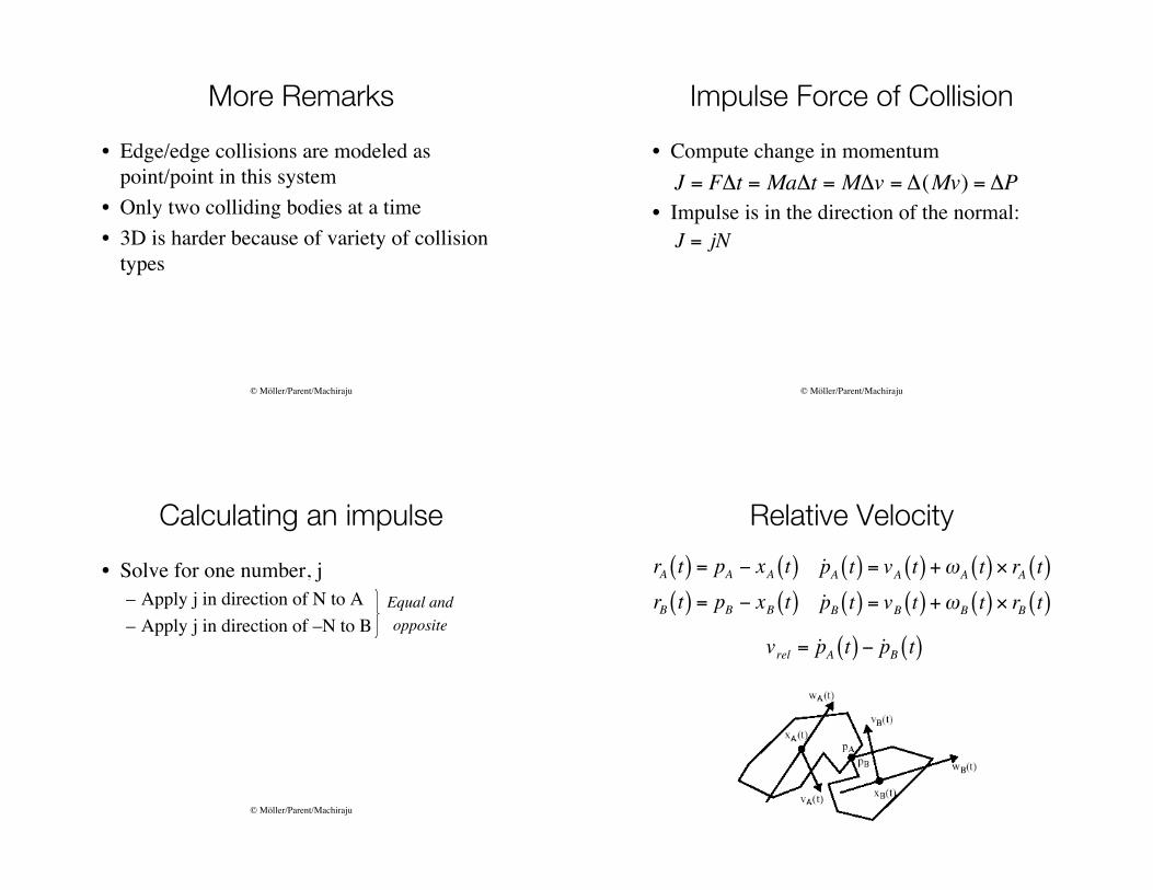
Relative Velocity
!
rA t( ) = pA " xA t( )
rB t( ) = pB " xB t( )
!
˙ p A t( ) = vA t( ) +"A t( ) # rA t( )
˙ p B t( ) = vB t( ) +"B t( ) # rB t( )
!
vrel = ˙ p A t( ) " ˙ p B t( )
© Möller/Parent/Machiraju
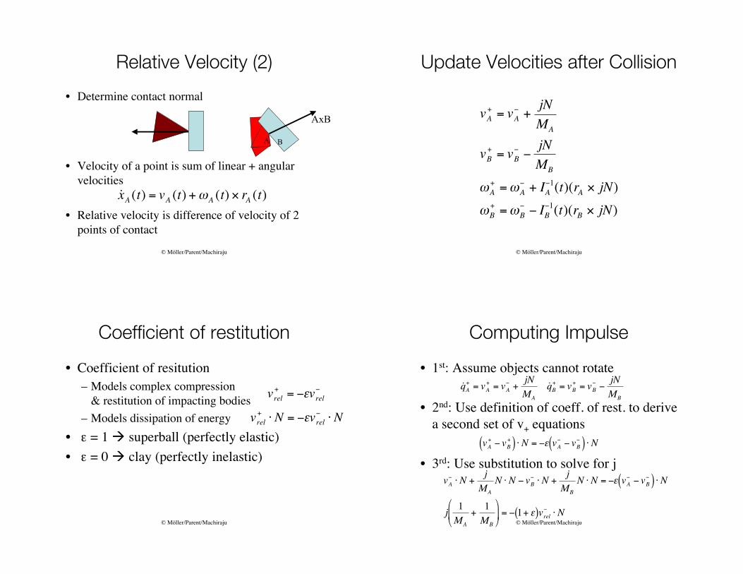
• Determine contact normal
• Velocity of a point is sum of linear + angular
velocities
• Relative velocity is difference of velocity of 2
points of contact
AxB
A B
!
˙ x A(t) = v
A(t) +"
A(t) # r
A(t)
Relative Velocity (2)
© Möller/Parent/Machiraju
Update Velocities after Collision
!
vA+ = vA
" +jN
MA
vB+
= vB""jN
MB
#A
+ =#A
" + IA"1(t)(rA $ jN)
#B
+=#B
"" IB
"1(t)(rB $ jN)
© Möller/Parent/Machiraju
!
vrel
+= "#v
rel
"
Coefficient of restitution
• Coefficient of resitution
– Models complex compression
& restitution of impacting bodies
– Models dissipation of energy
• # = 1 " superball (perfectly elastic)
• # = 0 " clay (perfectly inelastic)
!
vrel
+" N = #$v
rel
#" N
© Möller/Parent/Machiraju
Computing Impulse
• 1st: Assume objects cannot rotate
• 2nd: Use definition of coeff. of rest. to derive
a second set of v+ equations
• 3rd: Use substitution to solve for j
!
vA" # N +
j
MA
N # N " vB" # N +
j
MB
N # N = "$ vA" " vB
"( ) # N
j1
MA
+1
MB
%
& '
(
) * = " 1+ $( )vrel
" # N
!
˙ q A+
= vA
+= vA
"+
jN
MA
˙ q B+
= vB
+= vB
""
jN
MB
!
vA
+" v
B
+( ) # N = "$ vA
"" v
B
"( ) # N
© Möller/Parent/Machiraju
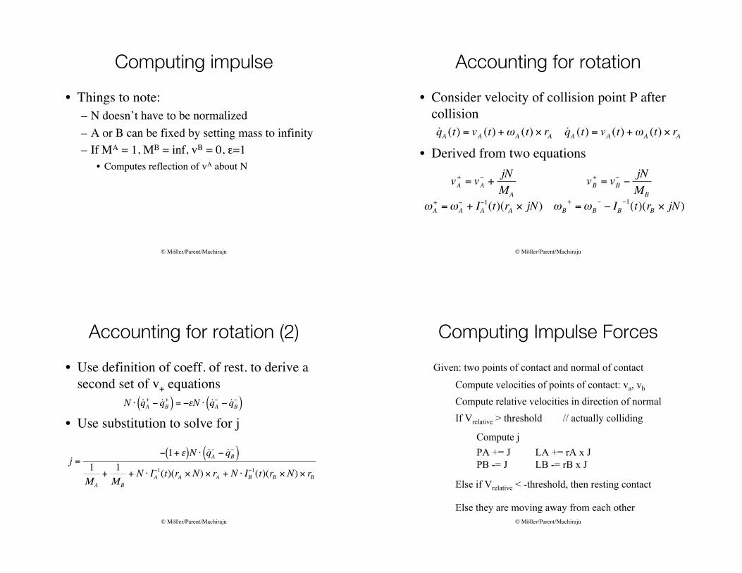
Computing impulse
• Things to note:
– N doesn’t have to be normalized
– A or B can be fixed by setting mass to infinity
– If MA = 1, MB = inf, vB = 0, #=1
• Computes reflection of vA about N
© Möller/Parent/Machiraju
• Consider velocity of collision point P after
collision
• Derived from two equations
Accounting for rotation
!
vA+
= vA"
+jN
MA
vB+
= vB""jN
MB
#A
+ =#A
" + IA"1(t)(rA $ jN) #B
+=#B
"" IB
"1(t)(rB $ jN)
!
˙ q A (t) = vA (t) +"A (t) # rA˙ q A (t) = vA (t) +"A (t) # rA
© Möller/Parent/Machiraju
Accounting for rotation (2)
• Use definition of coeff. of rest. to derive a
second set of v+ equations
• Use substitution to solve for j
!
N " ˙ q A+# ˙ q B
+( ) = #$N " ˙ q A## ˙ q B
#( )
!
j =" 1+ #( )N $ ˙ q A
"" ˙ q B
"( )1
MA
+1
MB
+ N $ IA
"1(t)(rA % N) % rA + N $ IB
"1(t)(rB % N) % rB
© Möller/Parent/Machiraju
If Vrelative > threshold // actually colliding
Compute velocities of points of contact: va, vb
Compute relative velocities in direction of normal
Given: two points of contact and normal of contact
Compute j
PA += J
PB -= J
LA += rA x J
LB -= rB x J
Else if Vrelative < -threshold, then resting contact
Else they are moving away from each other
Computing Impulse Forces