Position-Based Rigid Body Dynamics

Crispin Deul, Patrick Charrier and Jan BenderGraduate School of Excellence Computational Engineering

Technische Universitat Darmstadt, Germany{deul | charrier | bender}@gsc.tu-darmstadt.de

AbstractWe propose a position-based approach for large-scale simulations of rigid bodies at interactiveframe-rates. Our method solves positional con-straints between rigid bodies and therefore inte-grates nicely with other position-based methods.Interaction of particles and rigid bodies throughcommon constraints enables two-way cou-pling with deformables. The method exhibitsexceptional performance and stability whilebeing user-controllable and easy to implement.Various results demonstrate the practicabil-ity of our method for the resolution of colli-sions, contacts, stacking and joint constraints.

Keywords: real-time, rigid body dynamics,two-way coupling, position-based dynamics

1 Introduction

Computer games and virtual reality applicationsstrive for ever greater realism in increasinglycomplex virtual environments. Such environ-ments typically include a vast number of dy-namic deformable and rigid objects. Simulatingthese objects according to the laws of motion re-quires sophisticated methods and has a long his-tory in computer graphics. In this context theanimation of rigid bodies and their interactionsunder the influence of constraints such as col-lisions or joints is perhaps the most researchedconcern. Numerous physics engines, like Bul-let [1] or PhysX [2] have come to public atten-tion. While many methods achieve results ofgreat fidelity, their computational effort can notbe justified in real-time applications. The quest

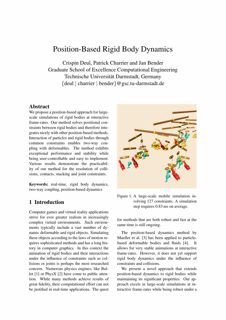
Figure 1: A large-scale mobile simulation in-volving 127 constraints. A simulationstep requires 0.83 ms on average.

for methods that are both robust and fast at thesame time is still ongoing.

The position-based dynamics method byMueller et al. [3] has been applied to particle-based deformable bodies and fluids [4]. Itallows for very stable animations at interactiveframe-rates. However, it does not yet supportrigid body dynamics under the influence ofconstraints and collisions.

We present a novel approach that extendsposition-based dynamics to rigid bodies whilemaintaining its significant properties. Our ap-proach excels in large-scale simulations at in-teractive frame-rates while being robust under a

vast number of constraints, as depicted in Fig-ure 1. Furthermore, the proposed method is easyto implement, controllable and supports two-way coupling of deformable and rigid bodies.

2 Related Work

The field of rigid body dynamics has a longhistory in computer animation and may be de-composed into the four subfields integrationschemes, collision detection, collision responseand constraint resolution. The survey of Benderet al. [5] describes all subfields in more detail,but only the two latter ones are of primary inter-est in this paper.

In previous work collision handling was per-formed by the application of forces [6], by solv-ing linear complementary problems [7] or by us-ing impulse-based methods [8, 9, 10]. Muller etal. [3] even introduce a method that resolves col-lisions by directly modifying positions for thesimplified case of individual particles. How-ever, an extension to rigid bodies has not beenshown yet. In contrast to that, Kaufman etal. [11] present a method which projects the ve-locities of the bodies in order to prevent pene-trations. Later, Kaufman et al. [12] introduceda staggering approach for frictional contacts.Multi-impact problems were focused by Smithet al. [13]. In order to increase the performanceof large-scale simulations, shock propagationmethods were introduced [9, 14]. Furthermore,different GPU-based methods were presented tosimulate large systems in real-time [15, 16].

To simulate an articulated system with joints,equality constraints are defined for the rigid bod-ies. A classic approach to solve these constraintsin real-time is to use reduced coordinate meth-ods. Featherstone demonstrated that a simula-tion with reduced coordinates can be performedin linear time for acyclic systems [17, 18]. Re-don et al. [6] introduced an adaptive variant ofthis approach which uses a reduced number ofdegrees of freedom to improve the performance.Baraff [19] introduced a Lagrange multipliermethod which also has a linear-time complex-ity for acyclic models. Later, Bender [20, 21]demonstrated that the idea of Baraff can alsobe applied to impulse-based simulation. WhileBender proposed to solve a linearized equation

based on a prediction of the joint state [22], We-instein et al. [23] solved the nonlinear equationby a Newton iteration method.

Position-based methods became popular inthe last years since they are fast, robust and con-trollable while no implicit time integration is re-quired. A survey of position-based methods ispresented by Bender et al. [24]. Muller et al. [3]introduced position-based dynamics as a gener-alized framework capable of solving a large va-riety of constraints. They demonstrated its ap-plication on deformable solids [3, 25] and lateralso on fluids [4]. Diziol et al. [26] introduceda shape matching method with a volume conser-vation for deformable solids to achieve more re-alistic results. In order to make shape matchingmore robust, Muller and Chentanez [25] addedan orientation to the particles of their model.This allows them to simulate bodies with solidcomponents and basic joints. Although theytreat each particle as a rigid body with posi-tion and orientation, they apply the standardposition-based constraints that depend solely onparticle positions. In constrast, our work incor-porates position and orientation in the deriva-tion of constraint equations. This allows usto form constraints between arbitrary points ofrigid bodies.

3 Preliminaries

In this section we first start with a brief intro-duction to the position-based dynamics frame-work (PBD). Then we continue with the basicsof rigid body simulation.

The original position-based dynamics ap-proach [3] is used to simulate a model definedby particles and constraints between these parti-cles. The constraints are solved at the positionlevel by applying correction displacements ontothe particle positions. In order to measure theconstraint violation, preview positions of theparticles are computed in a first step by integrat-ing the particle velocities under the influenceof external forces. Then the particle positionsare integrated with the new velocities yielding asymplectic Euler scheme. In the second step thesystem of constraints is solved in a Gauss-Seideltype iteration. The third step updates the particlevelocities depending on the difference between

the particle positions at the start of the time stepand the new particle positions multiplied by theinverse time step size. In a final step the newvelocities are modified to handle friction anddamping.

As mentioned before, we want to solve con-straints on rigid bodies, which are defined by sixparameters. The translational motion parame-ters are the position x, the velocity v, and themass m, which rigid bodies have in commonwith particles. In addition to that, the three ro-tational parameters are the orientation ϑ, the an-gular velocity ω, and the inertia tensor I.

These parameters are employed in a symplec-tic Euler scheme as follows. The equations forvelocity and position integration are defined by

v(t0 + h) = v(t0) +Fexternal

mh

x(t0 + h) = x(t0) + v(t0 + h)h

while the equations for the rotational parametersare given by

ω(t0 + h) = ω(t0) + hI−1·(τ external − (ω(t)× (I · ω(t))))

q(t0 + h) = q(t0) +h

2ω(t0 + h) · q(t0),

where ω is the quaternion [0, ωx, ωy, ωz]. Af-ter the preview positions of the bodies are in-tegrated with the equations above position con-straints are solved in several iterations. How-ever, in constrast to the original PBD approach,that updates the velocities after the constraintsolver step, we update the velocities of con-straints whenever a correction displacement isapplied to a rigid body. The required impulse toupdate the velocities is computed be multiplyingthe mass weighted displacement with the inversetime step size. By updating the velocities duringthe position iterations we can apply our frictionresolution approach whose details are presentedin section 6.

4 Constrained Rigid Bodies

In this section we describe how to extend thePBD solver to solve constraints between rigidbodies. The standard solver works by itera-tively handling each constraint on its own by

applying displacements to the according parti-cles. The displacements are computed by solv-ing constraints of the following form:

C(p + ∆p) = 0, (1)

where p = [p1, . . . ,pn]T is the concatenatedvector of particle preview positions and ∆p =[∆p1, . . . ,∆pn]T contains the correspondingcorrection displacements.

In order to solve a constraint function a first-order Taylor approximation

C(p+∆p) ≈ C(p)+∇pC(p) ·∆p = 0, (2)

is used to linearize the constraint. However, thisequation is underdetermined. By restricting thedirection of the position correction to the gra-dient direction this problem is solved [3]. Thefinal displacement vector is determined by

∆pi = − wiC(p)∑j wj

∣∣∣∇pjC(p)

∣∣∣2∇piC(p), (3)

where wi is the inverse mass of particle pi.As an extension to the particle constraint han-

dling of PBD our approach handles constraintsbetween rigid bodies. In contrast to particles anorientation is associated to rigid bodies. Pointspi that are attached to a rigid body with index jcan be described by the following formula

pi(xj ,R(ϑj)) = xj + R(ϑj)ri, (4)

where xj is the center of mass and R(ϑj) the ro-tation matrix of the rigid body with index j. Thelocal position of the point i in the body frameis encoded in ri. Using the definition of bodyattached points (see Eq. 4) in the Taylor approx-imation of the constraint (see Eq. 2) yields:

C(p(x + ∆x,R(ϑ+ ∆ϑ))) ≈C(p(x,R(ϑ)))+

JC(x, ϑ) · [∆xT1 ,∆ϑ

T1 , . . . ,∆xT

n ,∆ϑTn ]T ,

(5)

where x = [xT1 , · · · .xT

n ]T and ϑ =[ϑT1 , · · · , ϑTn ]T are the vectors containing allpositions and orientations of the n constrainedbodies. Furthermore, the function p com-putes the concatenated vector of m positionsp = [p1(x1,R(ϑ1))

T , . . . ,pm(xn,R(ϑn))T ]T

that are constrained by C(p). Due to the fact,

that the entries of p depend on a function (seeEq. 4), the chain rule has to be applied tothe constraint function C(p) to compute itsderivative. As a result, the gradient ∇pC(p)in Eq. 2 is replaced by the k × 6n JacobianJC(x, ϑ) =

(∂C∂x

∂C∂ϑ

)of the constraint function

with respect to the rigid body positions andorientations, where k is the dimension of thecodomain of C(p).

Let Mj be the 6×6 mass matrix of rigid bodyj with the mass on the first three entries of thediagonal and the moment of inertia tensor Ij inthe lower right 3 × 3 submatrix. By rearrang-ing Eq. 5 the same way that led from Eq. 2 toEq. 3 and replacing the inverse particle mass wj

with the inverse mass matrix M−1j , the formula

to compute the vector of rigid body correctionsfor constraint C(p) is:

[∆xTi ,∆ϑ

Ti , . . . ,∆xT

n ,∆ϑTn ]T =

−M−1JTC

[JCM−1JT

C

]−1C(p),

(6)

where the matrix M−1JTC converts the mass

weighted displacement to a displacement inworld space. The matrix

[JCM−1JT

C

]−1is the

mass matrix in constraint space.The question now is how to parameterize the

rotations of the rigid bodies to compute a Jaco-bian JC that can be multiplied with the inversemass matrix M−1

j . Orientations can be param-eterized in different ways like Euler angles orquaternions. Accordingly, all these parameteri-zations lead to a different Jacobian. Neverthe-less, a solution can be found by starting at thevelocity level. The relationship between angu-lar momentum and angular velocity is L = Iω.Taking the first order integration, with the as-sumption that the axis of rotation stays constantduring the time step, and rearranging the resultgives I−1Lh = ωh = ϑ, where h is the timestep size. The vector ϑ represents a rotation of|ϑ| about the axis ϑ/ |ϑ| and is known as the ex-ponential map from R3 to S3 [27], where S3 isthe space of rotation quaternions . The paper ofGrassia [27] also presents the derivation of therotational part ∂R(ϑ)/∂ϑ of the Jacobian JC

which is not repeated here.

5 Joints

Defining translational joint constraints betweentwo rigid bodies is straight forward using theconstraint definition of section 4. The transla-tional constraints have in common that the dis-tance of two joint points a and b, each attachedto one of the two bodies A and B, is constrainedto be zero. The only difference is the dimensionof the constraint space. A simple translationalconstraint is the ball joint

C(a,b) = a− b = 0

that removes all translational degrees of freedombetween the linked bodies. It follows that thejoint points and with them the according bodiescan not move away from each other. However,the two bodies can freely rotate around the jointposition. In order to define a translational con-straint that removes only two translational de-grees of freedom the constraint space has to bereduced to a plane. The plane is defined by thejoint point of one of the two bodies and the planenormal that is also attached to this body. It fol-lows that the joint points have to be projectedinto the plane to measure the constraint viola-tion. Then, the correction is computed in thetwo-dimensional constraint space. In a final stepthe mass weighted correction displacement mustbe projection back into the three-dimensionalspace. Similarly, the constraint space of a jointconstraining one translational degree of freedomis defined by attaching a unit vector to one of therigid bodies. Again, the constraint violation ismeasured by first projecting the joint points ontothe constraint space and then computing the dis-tance.

Constraints that remove only rotational de-grees of freedom can be defined analogously byconstraining the orientation of the linked bodies.

6 Collision Handling

In this section we present our solution to handlecollisions, contact, and friction. In the follow-ing paragraphs we combine the terms collisionand contact under the term proximity and usethe special terms only where differences occur.

Proximity Detection We perform only onediscrete proximity detection step to ensure a

high performance of our method. The drawbackis that, intersections may occur after the posi-tion integration or during the position solver it-erations. These intersections are corrected in thenext time step. It follows that, we can not guar-antee an intersection free state at the end of thetime step. But, we did not encounter severe ar-tifacts in our examples. A further implicationof performing only one collision detection stepis, that we need to classify proximity constraintsinto collisions or contacts by using a thresholdvelocity. Therefore, we apply the threshold pro-posed by Mirtich [8].

Intersection resolution Intersections of rigidbodies are handled during the position solver it-erations. If an intersection between bodies Aand B is detected, a proximity constraint is cre-ated. Let n be the intersection normal definedby the surface normal of body B. In order tosolve the intersection, a displacement has to becomputed that moves the intersection point a ofbody A along the positive direction of the inter-section normal and moves the intersection pointb of body B along the negative direction of theintersection normal. The constraint is given by

C(a,b) = nT (a− b) ≥ 0.

It follows that the constraint formula resemblesa distance constraint along the intersection nor-mal. The exception to the distance constraintis, that the displacements should be only repul-sive. To ensure that the total displacement of theconstraint stays repulsive during the solver iter-ations, every intersection constraint tracks thesum of the already applied displacements. Ifthe sum from the previous steps with the currentdisplacement in iteration step i becomes smallerthan zero ∆pcorrected = −

∑i−1j=1 ∆pj corrects

the displacement.A problem that arises when correcting the

whole intersection in a single time step is, thatobjects of the scene might receive an unwantedhigh velocity change, when deep intersectionsoccur. The intersections either are the resultof high body velocities in combination with thediscrete collision detection or they are causedby the position corrections in the previous timestep. Therefore, we use a stiffness parameter sas introduced in the original PBD approach also

for proximity constraints. Furthermore, to avoideven deeper penetrations caused by the correc-tion of other constraints, the required correctiondisplacement is split into two parts. Before per-forming the position solver iterations the currentintersection depth d is computed. In additiond is clamped to negative values including zerod = min(d, 0) to avoid cases when the colli-sion detection finds a collision due to the colli-sion tolerance value while the colliding objectsdo not intersect. Then, during each iteration stepthe current constraint violation value c is modi-fied as follows:

cmodified = min(0, c− d) + s ·max(c, d).

The first term is unequal to zero if a deeper inter-section than the initial intersection is computed.The second term corrects the initial intersectiondepth. In this equation the max function is used,because c and d are negative values in case of anintersection.

After performing the position correction it-erations a shock propagation method similar tothe approach of Guendelman [9] corrects the re-maining violated proximity constraints.

Friction Besides solving or preventing inter-sections, a plausible rigid body simulation alsohas to handle friction and collisions. Coulomb’sfriction model can easily be expressed in the ve-locity domain. Therefore, we compute frictioneffects at the velocity level. Furthermore, weapply a second friction approximation at the po-sition level to correct changes in tangential ve-locity of objects in proximity caused by positioncorrection constraints.

At the velocity level a Gauss-Seidel typesolver iterates over all proximity constraints infive iterations to handle contact, collision andfriction constraints. This is done immediatelyafter the velocity integration and before the po-sition integration of rigid bodies. As a result, anobject under static friction on an inclined planewill nearly stay at the same position. Withoutthis velocity correction, the object would moveunder gravity. As a result, the position correc-tion would push the object out of the plane alongthe plane normal. And finally the uncorrectedposition change tangential to the inclined planewould cause the object to slide.

The second stage of friction correction takesplace during the position correction iterations.Although the position constraint solver workswith weighted displacements we apply the fric-tion corrections as impulses to reuse the samefriction handling as at the velocity level. Inorder to compute the friction impulse the cur-rent velocity between the objects in contact isneeded. As a result of our velocity update imme-diately after a displacement has been applied inthe position iterations, the current tangential ve-locity is available for each proximity constraint.Then the friction impulse is computed to re-duce the tangential velocity. This impulse is cor-rected to lie in the friction cone before being ap-plied to the rigid bodies. It follows that the im-pulse along the intersection normal is requiredto correct the friction impulse. Therefore, wesum up the mass weighted displacements of theproximity constraints during the position correc-tion step. Then the mass weighted displace-ment is multiplied with the inverse time stepsize. Thus, an approximation for the impulse inthe direction of the intersection normal is com-puted. This impulse is used in conjunction withthe friction law to correct the friction impulse.

7 Two-way Coupling

A main advantage of integrating rigid body sim-ulation in the PBD framework is to gain stabletwo-way coupling between rigid bodies and de-formable models simulated with particles. Thealternative of using for example an impulsebased framework for the rigid bodies and in-terleaving the simulation with a PBD simula-tion may lead to stability issues. The problemwith interleaving is, that both simulations do not”see” constraints induced by the other frame-work.

With the extension of PBD constraints to han-dle rigid bodies like in section 4 it is very easyto couple rigid bodies and particles with a sin-gle constraint by using the concept of connec-tors introduced by Witkin et al. [28]. The idea isto split the Jacobian JC into a constraint and a

connector part. For a rigid body the splitting is

JC =∂C(p(x,R(v)))

∂p(x,R(v))·(

∂p(x,R(v))

∂x

∂p(x,R(v))

∂v

)T

,

where the first factor is the constraint Jacobianwith respect to the constrained points and thesecond factor is the rigid body connector Jaco-bian. Besides rigid bodies also particles can behandled by Eq. 4. Therefore, the Jacobian has tobe computed with respect to the position param-eter x of the particle. As a result the splittingis

JC =∂C(p)

∂p

∂p

∂x=∂C(p)

∂p.

The particle connector Jacobian ∂p/∂x is theidentity matrix. Furthermore, the mass matrixof the rigid body has to be exchanged with the3×3 particle mass matrix containing the particlemass on each of the diagonal elements. To sumup, by using the concept of connectors, pointsdefined on rigid bodies and points defined byparticles can be simultaneously used in positionconstraints. Consequently a full two-way cou-pling is achieved.

8 Results

We tested our algorithm on a total of four exam-ples that are shown in the accompanying video:

1. The mobile example in Figure 1 demon-strates the exceptional stability of a sys-tem under a large number of constraints.Figure 4 shows that the average computa-tion times scale linearly with the numberof bodies.

2. A cloth example, exemplifying the two-way interaction between deformable andrigid bodies (see Figure 3). A number oftori deform the cloth by dropping on it.They react on the cloth’s response, but set-tle in a steady and jitter-free state after afew seconds.

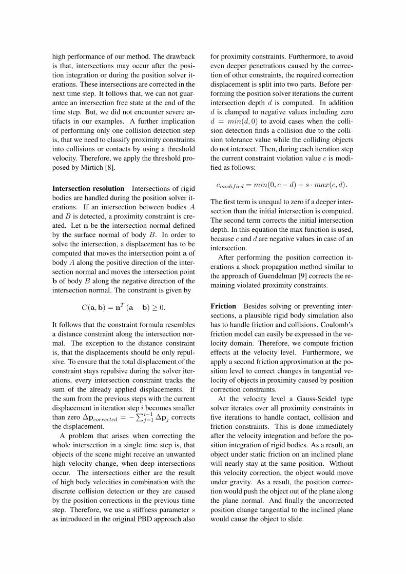
3. A pile example (see Figure 2) involving amassive number of collisions between twotypes of dropped rigid bodies with each

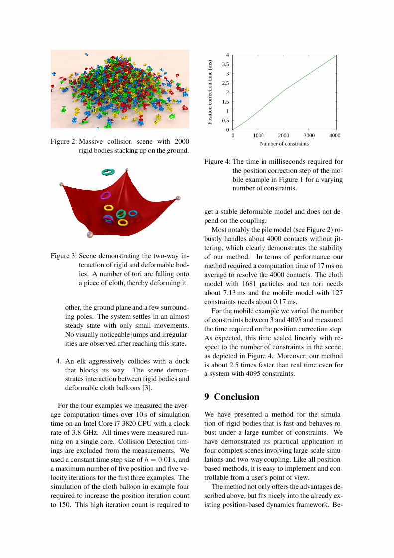
Figure 2: Massive collision scene with 2000rigid bodies stacking up on the ground.

Figure 3: Scene demonstrating the two-way in-teraction of rigid and deformable bod-ies. A number of tori are falling ontoa piece of cloth, thereby deforming it.

other, the ground plane and a few surround-ing poles. The system settles in an almoststeady state with only small movements.No visually noticeable jumps and irregular-ities are observed after reaching this state.

4. An elk aggressively collides with a duckthat blocks its way. The scene demon-strates interaction between rigid bodies anddeformable cloth balloons [3].

For the four examples we measured the aver-age computation times over 10 s of simulationtime on an Intel Core i7 3820 CPU with a clockrate of 3.8 GHz. All times were measured run-ning on a single core. Collision Detection tim-ings are excluded from the measurements. Weused a constant time step size of h = 0.01 s, anda maximum number of five position and five ve-locity iterations for the first three examples. Thesimulation of the cloth balloon in example fourrequired to increase the position iteration countto 150. This high iteration count is required to

0

0.5

1

1.5

2

2.5

3

3.5

4

0 1000 2000 3000 4000

Posi

tion

corr

ectio

n tim

e (m

s)

Number of constraints

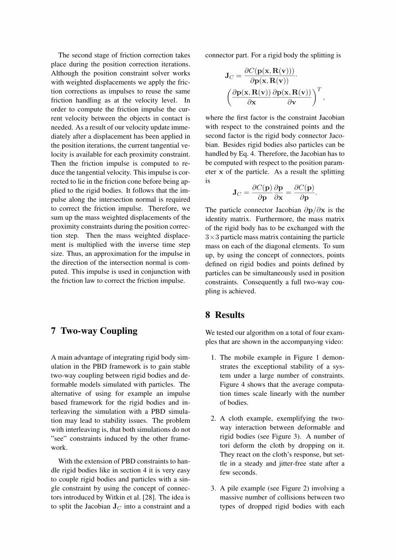
Figure 4: The time in milliseconds required forthe position correction step of the mo-bile example in Figure 1 for a varyingnumber of constraints.

get a stable deformable model and does not de-pend on the coupling.

Most notably the pile model (see Figure 2) ro-bustly handles about 4000 contacts without jit-tering, which clearly demonstrates the stabilityof our method. In terms of performance ourmethod required a computation time of 17 ms onaverage to resolve the 4000 contacts. The clothmodel with 1681 particles and ten tori needsabout 7.13 ms and the mobile model with 127constraints needs about 0.17 ms.

For the mobile example we varied the numberof constraints between 3 and 4095 and measuredthe time required on the position correction step.As expected, this time scaled linearly with re-spect to the number of constraints in the scene,as depicted in Figure 4. Moreover, our methodis about 2.5 times faster than real time even fora system with 4095 constraints.

9 Conclusion

We have presented a method for the simula-tion of rigid bodies that is fast and behaves ro-bust under a large number of constraints. Wehave demonstrated its practical application infour complex scenes involving large-scale simu-lations and two-way coupling. Like all position-based methods, it is easy to implement and con-trollable from a user’s point of view.

The method not only offers the advantages de-scribed above, but fits nicely into the already ex-isting position-based dynamics framework. Be-

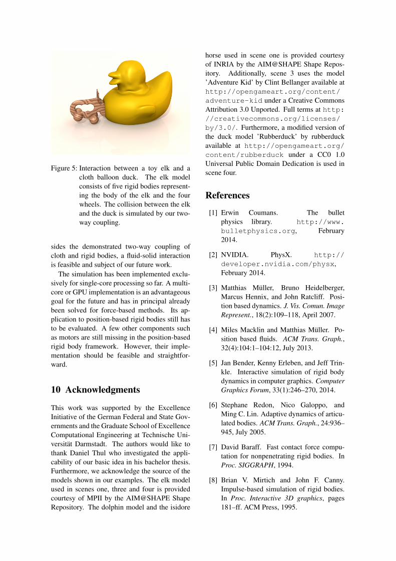
Figure 5: Interaction between a toy elk and acloth balloon duck. The elk modelconsists of five rigid bodies represent-ing the body of the elk and the fourwheels. The collision between the elkand the duck is simulated by our two-way coupling.

sides the demonstrated two-way coupling ofcloth and rigid bodies, a fluid-solid interactionis feasible and subject of our future work.

The simulation has been implemented exclu-sively for single-core processing so far. A multi-core or GPU implementation is an advantageousgoal for the future and has in principal alreadybeen solved for force-based methods. Its ap-plication to position-based rigid bodies still hasto be evaluated. A few other components suchas motors are still missing in the position-basedrigid body framework. However, their imple-mentation should be feasible and straightfor-ward.

10 Acknowledgments

This work was supported by the ExcellenceInitiative of the German Federal and State Gov-ernments and the Graduate School of ExcellenceComputational Engineering at Technische Uni-versitat Darmstadt. The authors would like tothank Daniel Thul who investigated the appli-cability of our basic idea in his bachelor thesis.Furthermore, we acknowledge the source of themodels shown in our examples. The elk modelused in scenes one, three and four is providedcourtesy of MPII by the AIM@SHAPE ShapeRepository. The dolphin model and the isidore

horse used in scene one is provided courtesyof INRIA by the AIM@SHAPE Shape Repos-itory. Additionally, scene 3 uses the model’Adventure Kid’ by Clint Bellanger available athttp://opengameart.org/content/adventure-kid under a Creative CommonsAttribution 3.0 Unported. Full terms at http://creativecommons.org/licenses/by/3.0/. Furthermore, a modified version ofthe duck model ’Rubberduck’ by rubberduckavailable at http://opengameart.org/content/rubberduck under a CC0 1.0Universal Public Domain Dedication is used inscene four.

References

[1] Erwin Coumans. The bulletphysics library. http://www.bulletphysics.org, February2014.

[2] NVIDIA. PhysX. http://developer.nvidia.com/physx,February 2014.

[3] Matthias Muller, Bruno Heidelberger,Marcus Hennix, and John Ratcliff. Posi-tion based dynamics. J. Vis. Comun. ImageRepresent., 18(2):109–118, April 2007.

[4] Miles Macklin and Matthias Muller. Po-sition based fluids. ACM Trans. Graph.,32(4):104:1–104:12, July 2013.

[5] Jan Bender, Kenny Erleben, and Jeff Trin-kle. Interactive simulation of rigid bodydynamics in computer graphics. ComputerGraphics Forum, 33(1):246–270, 2014.

[6] Stephane Redon, Nico Galoppo, andMing C. Lin. Adaptive dynamics of articu-lated bodies. ACM Trans. Graph., 24:936–945, July 2005.

[7] David Baraff. Fast contact force compu-tation for nonpenetrating rigid bodies. InProc. SIGGRAPH, 1994.

[8] Brian V. Mirtich and John F. Canny.Impulse-based simulation of rigid bodies.In Proc. Interactive 3D graphics, pages181–ff. ACM Press, 1995.

[9] Eran Guendelman, Robert Bridson, andRonald Fedkiw. Nonconvex rigid bodieswith stacking. ACM Trans. Graph., 2003.

[10] Jan Bender and Alfred Schmitt.Constraint-based collision and con-tact handling using impulses. In Proc.Computer Animation and Social Agents,pages 3–11, 2006.

[11] Danny M. Kaufman, Timothy Edmunds,and Dinesh K. Pai. Fast frictional dynam-ics for rigid bodies. ACM Trans. Graph.,24(3):946–956, 2005.

[12] Danny M. Kaufman, Shinjiro Sueda,Doug L. James, and Dinesh K. Pai. Stag-gered projections for frictional contact inmultibody systems. ACM Trans. Graph.,27(5), 2008.

[13] Breannan Smith, Danny M. Kaufman, Eti-enne Vouga, Rasmus Tamstorf, and EitanGrinspun. Reflections on simultaneous im-pact. ACM Trans. Graph., 31(4):106:1–106:12, July 2012.

[14] Kenny Erleben. Velocity-based shockpropagation for multibody dynamics an-imation. ACM Trans. Graph., 26(2):12,2007.

[15] A. Tasora, D. Negrut, and M. Anitescu.Large-scale Parallel Multi-body Dynamicswith Frictional Contact on the GraphicalProcessing Unit. In Proc. of Institution ofMech. Eng., Part K: Journal of Multi-bodyDynamics, pages 315–326, 2008.

[16] Daniel Weber, Jan Bender, Markus Sch-noes, Andre Stork, and Dieter Fellner. Ef-ficient GPU data structures and methodsto solve sparse linear systems in dynamicsapplications. Computer Graphics Forum,32(1):16–26, 2013.

[17] Roy Featherstone and David Orin. Robotdynamics: Equations and algorithms. In-ternational Conference on Robotics andAutomation, pages 826–834, 2000.

[18] Roy Featherstone. Rigid Body DynamicsAlgorithms. Springer-Verlag New York,Inc., Secaucus, USA, 2007.

[19] David Baraff. Linear-time dynamics usinglagrange multipliers. In Proc. SIGGRAPH,pages 137–146. ACM Press, 1996.

[20] Jan Bender. Impulse-based dynamic sim-ulation in linear time. Computer Anima-tion and Virtual Worlds, 18(4-5):225–233,2007.

[21] Jan Bender. Impulsbasierte Dynamiksim-ulation von Mehrkorpersystemen in dervirtuellen Realitat. PhD thesis, Universityof Karlsruhe, Germany, 2007.

[22] Jan Bender, Dieter Finkenzeller, and Al-fred Schmitt. An impulse-based dynamicsimulation system for VR applications. InProc. Virtual Concept. Springer, 2005.

[23] Rachel Weinstein, Joseph Teran, and RonFedkiw. Dynamic simulation of articu-lated rigid bodies with contact and colli-sion. IEEE TVCG, 12(3):365–374, 2006.

[24] Jan Bender, Matthias Muller, Miguel A.Otaduy, and Matthias Teschner. Position-based methods for the simulation of solidobjects in computer graphics. In EURO-GRAPHICS State of the Art Reports. Eu-rographics Association, 2013.

[25] Matthias Muller and Nuttapong Chen-tanez. Solid simulation with oriented par-ticles. ACM Trans. Graph., 30(4):92:1–92:10, July 2011.

[26] Raphael Diziol, Jan Bender, and DanielBayer. Robust real-time deformation ofincompressible surface meshes. In Proc.ACM SIGGRAPH/Eurographics Sympo-sium on Computer Animation. Eurograph-ics Association, 2011.

[27] F. Sebastian Grassia. Practical parameter-ization of rotations using the exponentialmap. Journal of Graphics Tools, 3:29–48,1998.

[28] Andrew Witkin, Michael Gleicher, andWilliam Welch. Interactive dynamics. InProc. Interactive 3D Graphics, pages 11–21. ACM, 1990.