rigid body dynamics - polito

Rigid Body Dynamics

If the aim of kinematics is to “describe” the body motion, the aim of dynamics isto “explain” it; the history of mechanics shows that the passage from description toexplanation requires the introduction of a new physical entity, that of mass or, inalternative, that of force.

The fundamental law of mechanics, due to Newton, is analytically expressed as avectorial equation between force, mass and acceleration of a translating rigid mass

f = ma or else

fxfyfz

= m

axayaz

where the linear acceleration a =

[ax ay az

]Tis a kinematic quantity, obtained

ad the time derivative of the body linear velocity.

This law is true in principle only for a single point-mass particle with mass m,where the applied force f and the acceleration a can exchange the role of cause andeffect: if a force f is applied to the particle, the particle accelerates with a linearacceleration equal to a , and conversely, if a particle has a linear acceleration a , theparticle is subject to a force f proportional to its mass.

If we jointly know the two vectors f =[fx fy fz

]Tand a =

[ax ay az

]T, we

can compute the mass from one or any of the following scalar relations as

m =fxax

=fyay

=fzaz

Though, in this last case, we are applying a circular argument, since no definitionsof “acceleration” or “force” exist that are independent from the measurement of amass; we are therefore compelled to use some trick, as clearly illustrated in [?].

If a single point mass is connected to others to form a rigid body, the Newton lawis still valid, given that we observe some precautions. Every point-mass shall beisolated and we must consider and deduce the forces applied on it by the othermasses; that is, we must introduce the constraint forces in addition to the externalforces applied on the body.

It is important to notice that the vector equations are dependent on the representa-tion used to characterize its components, and change changing the reference frame

1

2

used to represent the force and acceleration vectors, although the masses, at leastin a non-relativistic motion state, do not vary changing the reference frame.

In this textbook we will use an analytical approach, as defined in [?], instead ofthe vectorial one due to Newton. We consider the multibody system as a systemin which the dynamical equations derive from a unifying principle that implicitlyincludes and generates these equations.

This principle is based on the fact that, in order to describe the motion of a multi-body system is sufficient to consider and use in a proper way some suitable scalarquantities; these were in origin called by Leibnitz vis viva and work function, nowa-days take the name of kinetic energy and potential energy.

They are an example of the so-called state functions, since to each value of the statevector1

This general principle takes the name of principle of least action ; it can beroughly described in the following way.

Let us consider the space Q of the generalized coordinates q ∈ Q, as sketched inFigure 8 for a two-dimensional space Q; let us assume that a particle starts itsmotion at time t1 in the state Q1 = q(t1) and ends it motion at time t2 havingreached the state Q2 = q(t2).

Let us further assume that the motion keeps constant the sum E = C + P of thekinetic energy C and the potential energy P that the particle has at time t1.

Given the continuity of motion, the two points Q1 and Q2 are connected by acontinuous path (or trajectory), as the one represented by a continuous line inFigure 8; this trajectory is called the true trajectory, and at least in principle, it isunknown, since it is exactly what we want to compute as the result of the dynamicalequation analysis. If we had chosen at random a different trajectory, with the onlycondition that the two boundary point remain fixed, and called this trajectory aperturbed trajectory, the chance to obtain exactly the true trajectory would havebeen minimal.

Now we ask what is that characterize the true trajectory with respect to all possibleother perturbed trajectories. Euler was the first mathematician to contribute tothe solution of this problem, but it was Lagrange that developed a complete theory,that was later extended by Hamilton: the true trajectory is the one that minimizesthe integral of the so-called vis-viva (i.e., two times the kinetic energy) of the entiremotion between Q1 and Q2. This integral is called action and has a constant andwell defined value for each perturbed trajectory at constant E .

The least action principle states that the nature “chooses”, among the infinitenumber of trajectories starting in q(t1) and ending in q(t2), the trajectory that

1The concept of state will be defined in Section XXX; for the moment we simply consider thatthe state corresponds to the two vectors q(t) and q(t).

3

Figure 1: True and perturbed trajectories in the configuration space Q.

minimizes the definite integral S of a particular state function C∗(q(t), q(t))2 thatdepends on the generalized coordinates q(t) and the generalized velocities, whereq(t)

S =

∫ t2

t1

C∗(q(t), q(t))dt (1)

In order to apply this principle it is therefore necessary to compute the trajectory inthe space Q that minimizes S. The integral in (1) is computed between the initialtime t1 and the final time t2 and must obey to the boundary constraints active atthese two times.

The minimization of a functional3 is based on a particular mathematical technique,called calculus of variations, whose illustration goes beyond the scope of thepresent text. The interested reader can find additional treatment in [?], AppendixD.

FARE APPENDICE?

The conditions that assure the attainment of the minimum of S provide a set ofdifferential equations that contain the first and second time derivatives of the qi(t);this set completely describes the system motion dynamics.

As a final comment, we can say that the least action principle makes use of a concept- the action - that overturns the usual representation of the physical system dynamics

2We will see later what this state function C∗ is.3A functional is a mapping between a function and a real number; the function shall be con-

sidered as a whole, i.e., not a single particular value; in this sense a functional is often the integralof the function, as in the above equation for S.

4

by means of a set of differential equations.

With some approximation we can say that the differential equations specify theevolution of a physical quantity as the result of infinitesimal increments of time orposition; summing up this infinitesimal variations we obtain the physical variablesat every instant, knowing only their initial value and possibly some initial derivative:we can say that the motion has a local representation.

On the contrary, the action characterizes the motion dynamics requiring only theknowledge of the states at the initial and final times; every intermediate value of thevariables can be determined by the minimization of the action, that is a global, ratherthan local, measure. In any case the implementation of the principle of least actionproduces as a result a set of differential equations, different from these obtained withthe local representation.

In the following Sections we will illustrate how to obtain these equations.

0.1 Point Mass System

Yo introduce the Lagrangian approach and compare it with the Newtonian approachwe must define some general physical entities

Let us start to consider a sate of N point masses mi, with i = 1, · · · , N), as schemat-ically represented inn Figure 2. These systems are called multi-point systems.

Figure 2: A system of N point masses mi. The position r i and the velocity v i arerepresented in a generic reference frame Rb.

Now we consider a pure rotation motion around a point O, that, for simplicity, isthe origin of the reference frame Rb; all vectors will be represented in this frame. Ifnecessary we indicate the vectors as r b

i , otherwise with r i.

The position of the generic mass mi is defined by the vector r i =[xi yi zi

]T. If

the rotation velocity of the system is given by the vector ω, every mass will acquire

0.1. POINT MASS SYSTEM 5

a linear velocity v i, as the result of the rotation, whose value is

v i(t) = ω(t)× r i(t) = S(ω(t))r i(t) (2)

We define the linear momentum4 p i(t) as the product between the mass mi andthe velocity v i(t)

p i(t) = miv i(t)

In this Chapter, the symbol p indicates the linear momentum an not the cartesianpose of a body or the position of a point, as in the preceding Chapters.

0.1.1 Moment of a Force

We briefly recall that, given a point mass located in a point P represented by thevector r in the reference frame R, and a force f applied to it, the moment of theforce with respect to a point O is given by the cross product

r × f = r ×mdv

dt= r × dp

dt(3)

where the terms on the right side arise from the Newton equation.

It is important to recall that the term “moment” indicates the cross product, whilethe term “momentum” indicates the vector p = mv .

Applying the derivative rules in (??) to the right end side of (3), we obtain

r × f = r × dp

dt=

d

dt(r × p)− dr

dt× p

=d

dt(r × p)− v × p︸︷︷︸

0

=dh

dt

where the last term is always zero, since the moment p and the linear velocity of thepoint mass v are always collinear, and where the vector h = r ×p is called angularmoment or moment of the momentum. Since the moment r × f is often referred asthe torque applied by the force with respect to the point O, we can write

τ =d

dth

Note the analogy

f =d

dtp = p

τ =d

dth = h

4In Italian quantita di moto (lineare).

6

that shows the relations between the generalized force/torque and the generalizedmomentum.

Figure 3: A point mass m with the applied force f and it linear moment p.

0.1.2 Angular Momentum and Inertia Matrix

Given a point O in space and a point mass mi with position r i, belonging to aset of point masses, we have define the angular momentum, or moment ofmomentum5 h i, as

h i(t) = r i(t)× p i(t) = r i(t)× (miv i(t))

Replacing (2) in the above relation and omitting for simplicity the time dependency,we obtain

h i = mi(r i × (ω × r i))

Summing up all the N point masses contributions, we have the total angular mo-mentum

h =N∑i=1

h i =∑i

mi(r i × (ω × r i)) (4)

Recalling from (??) that the triple cross product enjoys of the following property

a × (b × c) = (aTc)b − (aTb)c,

where aTc and aTb are scalar products, it follows that the momentum can bewritten as

h =∑i

mi

((rT

i r i)ω − (rTi ω)r i

)5In Italian momento della quantita di moto or quantita di moto angolare.


Replacing with r2i the square norm ∥r i∥2 = rTi r i = (x2

i + y2i + z2i ) and writingexplicitely rT

i ω = (xiωx + yiωy + ziωz) we obtain

h =∑i

mi

r2i

ωx

ωy

ωz

− (xiωx + yiωy + ziωz)

xi

yizi

or

h =

hx

hy

hz

=∑i

mi(r2i − x2

i )ωx −mixiyiωy −mixiziωz

−mixiyiωx +mi(r2i − y2i )ωy −miyiziωz

−mixiziωx −miyiziωy +mi(r2i − z2i )ωz

(5)

This relation can be written in matrix form as

h =∑i

Γxx,i Γxy,i Γxz,i

Γyx,i Γyy,i Γyz,i

Γzx,i Γzy,i Γzz,i

ωx

ωy

ωz

=∑i

Γ iω (6)

where

Γxx,i = mi(r2i − x2

i ) = mi(y2i + z2i )

Γyy,i = mi(r2i − y2i ) = mi(x

2i + z2i )

Γzz,i = mi(r2i − z2i ) = mi(x

2i + y2i )

and

Γxy,i = Γyx,i = −mixiyi

Γxz,i = Γzx,i = −mixizi

Γyz,i = Γzy,i = −miyizi

If we now introduce a new matrix defined as

Γ =

Γxx Γxy Γxz

Γyx Γyy Γyz

Γzx Γzy Γzz

=∑i

Γxx,i Γxy,i Γxz,i

Γyx,i Γyy,i Γyz,i

Γzx,i Γzy,i Γzz,i

=∑i

Γ i

from (6) we have

h =

Γxx Γxy Γxz

Γyx Γyy Γyz

Γzx Γzy Γzz

ωx

ωy

ωz

= Γω (7)

or better, restating the time dependency

h(t) = Γ (t)ω(t)

8

The matrix Γ is called inertia matrix or inertia tensor and has on the maindiagonal the inertia moments

Γxx =∑i

mi(r2i − x2

i ) =∑i

mi(y2i + z2i ) =

∑i

mid2x

Γyy =∑i

mi(r2i − y2i ) =

∑i

mi(x2i + z2i ) =

∑i

mid2y (8)

Γzz =∑i

mi(r2i − z2i ) =

∑i

mi(x2i + y2i ) =

∑i

mid2z

and outside the diagonal the inertia products

Γxy = Γyx = −∑i

mixiyi

Γxz = Γzx = −∑i

mixizi (9)

Γyz = Γzy = −∑i

miyizi

Inertia moments

As one can notice, the inertia moments are obtained summing the contribu-tions of the products of each mass by the square euclidean distance d2x, d

2y, d

2z

from the three axes x, y and z.

Prodotti d’inerzia

When the inertia products are zero, the inertia matrix becomes diagonal

Γ =

Γxx 0 00 Γyy 00 0 Γzz

In this case the reference frame axes are aligned along what are called theprincipal inertia axes of the body, and the matrix is the so called principalinertia matrix.

Another possible representation of h and Γ can be obtained using (4) and theproperties of the skew-symmetric matrices:

h =∑i

mi(r i × (ω × r i)) =∑i

miS(r i)S(ω)r i (10)

Recalling that S(ω)r i = −S(r i)ω, one obtains:

h =∑i

miS(r i)S(ω)r i =∑i

−miS(r i)S(r i)ω (11)


and being ω a common term, at the end one has

h =

(−∑i

miS(r i)S(r i)

)ω = Γω (12)

withΓ = −

∑i

miS(r i)S(r i) (13)

The inertia matrix Γ depends on the r i vectors that characterize the positions ofthe masses mi in a given reference frame, with respect to a given point; this pointcan be fixed, as the origin O of the frame, or mobile (i.e., local) as the center of massC of the body; in the first case the inertia matrix will be indicated as Γ o, in thesecond case as Γ c.

Considering two reference frames with a common origin, but one rotated with respectto the other, the inertia matrices will be different; the rule to transform one into theother will be detailed later on.

The inertia matrix Γ represents the inertial properties of a rigid body subject to arotation, in the same way as the mass represents the inertia properties of a bodysubject to a translation.

Equation (7) is qualitatively similar to the expression of the total linear momentump(t) = mv(t). Since we can write it as p(t) = Mv(t), where M = mI , the twomomentum are

p(t) = Mv(t)

h(t) = Γ (t)ω(t)

with the difference that usually the mass matrix M does not depend on time, whileΓ (t) does.

Example 0.1.1

Let us consider a simple body system composed by two equal masses as in Figure4; we want to compute the angular momenta and the inertia matrices with respectto the points O and C.

Assume also that Ra is fixed, while Rb is on the barycenter (or center of mass) of

the body having the axis i aligned with the segment−−→CB.

Assume

r 1 =

120

; r c =

220

; r 2 =

320

; c1 =

−100

; c2 =

100

10

Figure 4: The two equal masses system considered in Example 0.1.1.

and m1 = m2 = 1.

Since Ra e Rb are parallel, the rotation matrix Rab = I and we can neglect it.

We start computing Γ o as

Γ o = −m1S(r 1)S(r 1)−m2S(r 2)S(r 2) =

8 −8 0−8 10 00 0 18

and then Γ c as

Γ c = −m1S(c1)S(c1)−m2S(c2)S(c2) =

0 0 00 2 00 0 2

Recalling the parallel axes theorem, that we will introduce in Paragraph 0.3.3, andassuming also (23) and (24), we obtain

Γ o − Γ c =

8 −8 0−8 8 00 0 16

= −(m1 +m2)S(r c)S(r c)

Now assuming that the angular velocity of the system is

ωaab = ωb

ab =

001

we can compute the momenta as follows

ho =

8 −8 0−8 10 00 0 18

001

=

0018

; h c =

0 0 00 2 00 0 2

001

=

002

�

0.2. DISTRIBUTED MASS SYSTEMS 11

0.2 Distributed Mass Systems

We make a further step assuming that the body whose angular moment we wantto compute is composed by a continuous distribution of infinitesimal point massesdm, having point density ρ(r) = ρ(x, y, z), depending on the position (x, y, z), andwhere the infinitesimal mass is dm = ρ(x, y, z)dV .

The coordinate r takes its values in V , where V is a finite space region that in-cludes the body, with a total volume V =

∫V dV and total mass mtot =

∫V dm =∫

V ρ(x, y, z)dV .

We can apply the same arguments used above for N point masses to a system ofdistributed masses, replacing in (8) and (9) the summation operator with the integraloperator in the volume V . We can now write in compact form the inertia matrix as:

Γ =

∫Vρ(x, y, z)

y2 + z2 −xy −xz−xy x2 + z2 −yz−xz −yz x2 + y2

dV (14)

obtaining the inertia moments

Γxx =

∫Vρ(r)(y2 + z2) dV

Γyy =

∫Vρ(r)(x2 + z2) dV (15)

Γzz =

∫Vρ(r)(x2 + y2) dV

and the inertia products

Γxy = Γyx = −∫Vρ(r)xy dV

Γxz = Γzx = −∫Vρ(r)xz dV (16)

Γyz = Γzy = −∫Vρ(r)yz dV

Notice that ρ(r)dV is equivalent to an infinitesimal mass dm(r), therefore we canalso write relation (14) as

Γ =

∫V

y2 + z2 −xy −xz−xy x2 + z2 −yz−xz −yz x2 + y2

dm(r) (17)

0.2.1 Some Observations

The inertia matrix is implicitly defined when we define the angular momentum has in (10); this one in turn is defined introducing a rotation around a point O,

12

characterized by the angular velocity ω.

The cartesian components of h are represented in the chosen reference frame, thatoften, but not always, coincides with a reference frame with its origin in O; theinertia matrix (or inertia tensor) describes the way the mass is distributed withrespect to the axes of R0(O; x, y, z). If the frame is rigidly attached to the body,the inertia matrix is time independent, otherwise it changes with time.

This is the reason why it is common to read in textbooks “inertia moment withrespect to a point” and/or “inertia matrix with respect to the axes”. This differenceshall not generate confusion since it is an example of a casual use of mathematicalconcepts, that, once understood, does not represents a problem anymore.

A reference frame attached to the body is called a body-frame and any inertiamatrix with respect to this frame is always constant.

If one chooses a different reference frame attached to the body, with the same ori-gin O, but different axes, the components of h do change and therefore also thecomponents of Γ , but they remain time-invariant.

If the frame is translated, Γ changes according to the parallel axes theorem (seeSection 0.3.3)

If the body rotates with respect to the reference frame (and therefore this one is nota body-frame), the components of Γ vary with time.

To conclude, we recall that what has been presented here is valid only for rigidbodies.

0.3 Mathematical Formulation

We have seen that a inertia matrix or tensor6 of a rigid body specifies and summarizethe inertial characteristics of the body with respect to the variations of the angularvelocity associated to the body rotation.

The matrix is always defined specifying explicitly or implicitly a point with respectto which it is computed; usually this point is the center of mass of the body, butthis choice it is not strictly necessary.

In order to define correctly the inertia matrix of a rigid body it is proper to introducea number of subscripts and superscripts that make clear the meaning with respectto the reference frames defined by the user.

Given a rigid body B, identified by the subscript b, and a reference system Rb, called

6The term tensor is used to indicate an abstract mathematical entity that generalizes thevectors, while we use the term matrix to indicate its representation in some defined referenceframe. We prefer to use “matrix” instead of “tensor” because it is more common in modelling andcontrol literature

0.3. MATHEMATICAL FORMULATION 13

local frame, the position of the center of mass C of the body is defined by thevector r b

c, computed as follows:

r bc

∫Bdm = r b

c mbtot =

∫Br bdm (18)

where r b represents the position in Rb of the generic point mass dm belonging tothe body B; moreover mb

tot =∫B dm is the total mass of the body B.

The inertia matrix Γ bc ∈ R3×3 around the center of mass C is defined, as seen in

Section 0.1.2, resorting to the angular momentum definition, that we write againhere, with the addition of the introduced subscripts and superscripts:

h bc = Γ b

cωb0 (19)

where h bc is the momentum of the rigid body with respect to C and ωb

0 ≡ ωb0b is the

total angular velocity of the rigid body; both are 3D vectors represented in Rb.

Take care not to confuse the total angular velocity ωb0b represented in Rb and the

same velocity represented in R0, that we shall indicate with the symbol ω00b.

The use of various subscripts and superscript in Γ bc is non a useless pedantry; on

the contrary it highlights the fundamental points of its definition: Γ bc is the inertia

matrix of the rigid body B with respect to its center of mass C, represented in thereference frame Rb, that in general can be placed everywhere one likes, but usuallyattached to the body. The inertia matrix changes changing the reference frame, aswe will see later.

If now we attach Rb to the rigid body with its origin in C we have from (18)

r bc = 0 →

∫Br bdm = 0 (20)

and the inertia matrix Γ bc will be defined as:

Γ bc = −

∫BS(r b)S(r b)dm =

∫B

[ ∥∥r b∥∥2 I − r b(r b)T

]dm

=

Γxx Γxy Γxz

Γyx Γyy Γyz

Γzx Γzy Γzz

(21)

where we notice that r b(r b)T is a rank one dyadic product (see Appendix ??), andthat S(x ) is a skew-symmetric matrix (see Appendix ??).

Observe the analogy of the second term in (21) with the second term in (13).

0.3.1 Rotation of the Reference Frame

If now we consider another reference frame Rk, rotated around the common origin(in this case C) with respect to Rb, and the rotation matrix given by Rk

b , then the

14

inertia matrix is computed according the following relation

Γ kc = Rk

bΓbcR

bk = Rk

bΓbc(R

kb )

T (22)

orΓ k

cRkb = Rk

bΓbc.

using the usual notation Rab = (Rb

a)T.

When the generic reference frame Rb is attached at the body B and moving withit, i.e., it is a body-frame, the inertia matrix relative to Rb is time invariant; in theother case it is time variant.

0.3.2 Principal Inertia Matrix

Often it is appropriate to refer to a “privileged” reference frame R∗, implicitlydefined as that frame having its origin in the body center of mass and with respectto which the inertia matrix is diagonal, i.e.,

Γ ∗c =

Γx 0 00 Γy 00 0 Γz

;

This frame has the three unit vectors i ∗, j ∗ andk ∗, aligned along the so-calledallineati principal inertia axes ; the matrix Γ ∗

c is called prende il nome di prin-cipal inertia matrix .

0.3.3 Parallel Axes Theorem

Assume that we know the inertia matrix with respect to a reference frame withorigin in the center of mass C, and we want to compute it with respect to anotherframe, with different origin O, but parallel axes.

To do so we must express the relation between the infinitesimal mass ρ dV = dmwith respect to the two points O e C is (vedi Fig. 6)

It is straightforward to see that:

r bi = r b

c + cbi , ∀i = 1, . . . , N

where r bc =

[tx ty tz

]Trepresents the translation of the reference frame from O to

C.

As we already know, the inverse translation, from C to O, is given by −r bc.

This relation is valid for any vector represented in a couple of translated referenceframes.

0.3. MATHEMATICAL FORMULATION 15

Figure 5: An example of parallel axes inertia computation.

The point mass element dmi that was in the position cbi , is now in position r b

i .

It is now possible to compute the new inertia matrix Γ bo, taking into account (21),

as

Γ bo = Γ b

c −mtotS(r bc)S(r b

c) = Γ bc +mtot

[∥∥r bc

∥∥2 I − r bc(r

bc)

T]

(23)

Simplifying the notation as follows

Γ bc ≡ Γ =

Γxx Γxy Γxz

Γyx Γyy Γyz

Γzx Γzy Γzz

e Γ bo ≡ Γ ′ =

Γ ′xx Γ ′

xy Γ ′xz

Γ ′yx Γ ′

yy Γ ′yz

Γ ′zx Γ ′

zy Γ ′zz

with t ≡ r b

c and with m ≡ mtot, we will obtain

Γ ′ = Γ −mS(t)S(t) (24)

= Γ +m[∥t∥2 I − ttT

]= Γ +m

(t2y + t2z) −txty −txtz−txty (t2x + t2z) −tytz−txtz −tytz (t2x + t2y)

that gives

Γ ′xx = Γxx +m

(t2y + t2z

)Γ ′yy = Γyy +m (t2x + t2z)

Γ ′zz = Γzz +m

(t2x + t2y

).

(25)

16

Figure 6: Parallel axes theorem: relation between the infinitesimal mass position inthe two cases.

The inertia products can be written as

Γ ′xy = Γxy −m txty

Γ ′xz = Γxz −m txtz

Γ ′yz = Γyz −m tytz

(26)

The two relations (22) and (23) allow to compute the inertia matrix with respect toany other point O of choice, knowing the inertia matrix with respect to the pointC.

The relation introduced above are valid both for discrete point-mass systems andfor distribute mass systems.

0.4 Angular Momentum and Euler Equation

The expression of the angular momentum has been introduced in (19) without anyadditional explanation; here we justify it in a more formal way.

We can assume that a rigid body B is composed by a continuum of point-massparticles with mass dm located at rk, with velocity v k = r k and acceleration ak =v k; the superscript k identifies the generic reference frame Rk with respect to whichthe vectors are represented. Since B is a rigid body, there will be a number ofconstraint relations linking positions, velocities and accelerations, as detailed inSection ??.

To simplify the mathematical treatment of the rigid body dynamics, we can reducethe action of the forces and torques acting on the body B to two equivalent effects:

0.4. ANGULAR MOMENTUM AND EULER EQUATION 17

• an equivalent linear force f kc , with its line of action across the body center

of mass C, and with a module equal to the module of the vector sum of theapplied forces;

• an equivalent torque τ kc , equal to the total moment of produced by the forces

acting on B, relative to C.

The second Newton Law states that the resulting inertial force is equal to thetime derivative of the linear momentum

f kc =

(d

dtmv k

c

)0

= m

(d

dtv kc

)0

= makc

where v kc is the instantaneous velocity of C, m is the total mass of the body and

akc = v k

c is the total acceleration of the center of mass; the relation is valid for anychoice of the reference frame Rk used to describe the vectors.

The Euler equation states that the inertial torque is equal to the time derivativeof the angular momentum

τ kc =

(d

dthk

c

)0

where in both cases we have pointed out that the total derivative must be performedwith respect to an inertial7 (or pseudo-inertial) reference frame R0; It is not neces-sary that Rk is an inertial frame, but only that the derivative, seen as the limit ofthe difference quotient between vectors, is computed in the inertial frame (see alsoSection ??).

The vector hkc is the angular momentum with respect to the mass center C and is

defined, in analogy to what has been introduce in Section 0.1.2, as follows:

hkc =

∫B(ck × v k)dm (27)

where ck indicates the position of an element of infinitesimal mass dm with respectto the center of mass C of the body (see also Figure 7).

Since the position of an element dm with respect to the origin O of the referenceframe Rk can be decomposed into the sum

rk = ck + r kc

it resultsck = r k − r k

c

where we have indicated with r kc the position of the center of mass C and with r k

the position of dm with respect to O.

7We recall that an inertial reference frame must be fixed or in linear uniform motion, i.e.,

18

Figure 7: The position rk of on infinitesimal mass element dm is decomposed intothe sum rk

c + ck. The reference frame Rk is assumed to be inertial and all vectorsare represented in it.

Corretto fin qua

Therefore, the velocity v k = r k of the generic elementary mass can be expressed inrelation to the velocity of the center of mass v k

c as follows

v k ≡ r k = ck + r kc = v k

c + ωkkb × ck (28)

The second term of the right hand side is obtained considering the relation (??),rewritten here for convenience comodita

r 0(t) = ω001(t)× ρ0(t) +R0

1r1(t) + d

0

1(t) (29)

where r 1(t) = d0

1(t) = 0, ρ0(t) ≡ ck and ωkkb ≡ ω0

01(t)

As usual, the angular velocity ωkkb, is the total angular velocity of B with respect to

Rk and is represented in Rk itself.

Replacing (28) in the (27), we obtain

hkc =

∫Bckdm× v k

c +

∫Bck × (ωk

kb × ck)dm =

the term∫B c

kdm goes to zero since, in accordance with the definition of the masscenter in (18), one can write:∫

Bckdm =

∫B(r k − r k

c )dm =

∫Br kdm−mr k

c = 0

one in which the accelerations acting on it are zero or negligible; in this last case the referenceframe is pseudo-inertial. For example, a reference frame on your study table experiences onlythe accelerations due to the Earth rotation around its axis and around the Sun, to neglect othermore complex motions of the Sun in the local galaxy, etc. In this textbook we call “inertial” anypseudo-inertial reference frame.

0.4. ANGULAR MOMENTUM AND EULER EQUATION 19

being∫r kdm = mrk

c

In conclusion, we have

hkc =

∫Bck × (ωk

kb × ck)dm = −∫Bck × (ck × ωk

kb)dm =

= −∫BS(ck)S(ck)ωk

kbdm = −∫BS(ck)S(ck)dm ωk

kb =

= definition (21) =

= Γ kcω

kkb

(30)

If we represent the vectors and the inertia matrix in a different reference frame Rℓ

we write

h ℓc = Γ ℓ

cωℓkb.

with the relation between the inertia matrices

Γ ℓc = Rℓ

kΓkcR

kℓ (31)

and the angular velocities

ωℓkb = Rℓ

kωkkb

therefore we can observe that

h ℓc = Γ ℓ

cωℓkb = Rℓ

kΓkc R

kℓR

ℓk︸︷︷︸

I

ωkkb = Rℓ

kΓkcω

kkb = Rℓ

khkc

To complete the Euler equation, we should define the time derivative of the angularmomentum. Recalling the expression (??), we can write

hk

c =

(d

dt

)0

(Γ kcω

kkb) =

(d

dt

)k

(Γ kcω

kkb) + ωk

cb × (Γ kcω

kcb)

Since Γ kc is a constant in Rk, it follows that

hk

b = Γ kbα

k0b + ωk

0b × (Γ kbω

k0b) (32)

where αk0b ≡ ωk

0b is the total angular acceleration of the body b represented in Rk.

In conclusion, the time derivative of the angular momentum, i.e., the inertial torquesthat appears in the Euler equation, can be simply written as:

h = Γ ω + ω × (Γω) (33)

where the simplified symbols are to be correctly interpreted.

20

Alternative Formulation

Another way to obtain (33) is the following: we assume that the body b rotates witha total angular velocity ω0 with respect to an inertial reference frame R0, whoseorigin is now located at the center-of-mass of the body.

The Euler equation, that describes the dynamics of a rotating body, states that thevariation of the angular momentum h0 is equal to the vector τ 0, that is the sum ofall torques applied to the body:

h0 ≡d

dt(Γ 0ω0) = τ 0 (34)

Both Γ 0 and ω0 are time functions, so we have

h0 = Γ 0ω0 + Γ 0ω0 (35)

In order to easily compute Γ 0 it is convenient to change the reference frame; if Rℓ

is the local frame attached to the body, i.e., the body-frame, having its origin in thecenter-of-mass, if R ≡ R0

ℓ is the rotation matrix representing Rℓ in R0, and if Γ ℓ

is the inertia tensor expressed in Rℓ, then we have seen from (22) that

Γ 0 = RΓ ℓRT (36)

Calling ωℓ the total angular velocity of the body represented in the frame Rℓ, i.e.,ωℓ ≡ ωℓ

0b, and calling ω0 the same velocity represented in R0, i.e., ω00b ≡ ω0, we

can write ω0 = Rωℓ and consequently

h0 = Γ 0ω0 = RΓ ℓRT Rωℓ = RΓ ℓωℓ = Rh ℓ (37)

where we have introduced the new vector h ℓ = Γ ℓωℓ that is the angular momen-tum represented in Rℓ. We can see that the angular momentum is a vector thattransforms from one reference frame to another with the same rule of other vectors.

Replacing h0 in (37) and computing the derivative, we obtain:

h0 =d

dt(RΓ ℓωℓ) = RΓ ℓωℓ +RΓ ℓωℓ +RΓ ℓωℓ (38)

The inertia tensor Γ ℓ is time invariant, since it is relative to a body-frame and thebody does not change its shape, therefore Γ ℓ = O , and (38) simplifies as follwos

h0 = S(ω0)RΓ ℓωℓ +RΓ ℓωℓ = ω0 × (RΓ ℓωℓ) +RΓ ℓωℓ (39)

This vector is represented inR0 but includes both ωℓ and ω0; if we want to representeverything in Rℓ we should pre-multiply by RT. Recalling the properties of theskew-symmetric matrices, we obtain

h ℓ = RTh0 = RTS(ω0)RΓ ℓωℓ +RTRΓ ℓωℓ

= S(RTω0)Γ ℓωℓ + Γ ℓωℓ

= S(ωℓ)Γ ℓωℓ + Γ ℓωℓ

= ωℓ × Γ ℓωℓ + Γ ℓωℓ

(40)

0.5. NEWTON-EULER EQUATIONS 21

Poiche h ℓ = τ ℓ, segue:τ ℓ = ωℓ × Γ ℓωℓ + Γ ℓωℓ (41)

where τ ℓ = RTτ 0 is the sum of the applied torques, represented in Rℓ.

If we prefer to represent the torque in R0, we use (39), replacing Γ 0R instead ofRΓ ℓ, obtained from (36); in this way we obtain

τ 0 = ω0 × Γ 0ω0 + Γ 0ω0 (42)

The equations (33), (41) and (42) are identical, provided that all vectors and tensormatrices are expressed in the same reference frame.

0.5 Newton-Euler Equations

The Newton-Euler equations are vector equilibrium equations that state that allforces and torques acting on the body B, including the inertial ones due to themotion, the external ones and those due to the constraint, are in (dynamical) equi-librium.

There are two vector equations, the first, due to Newton, describes the equilibriumof the linear forces, while the second, due mainly to Euler, describes the equilibriumof the linear momenta.

Assuming that the rigid body is connected with other rigid bodies, we must consideralso the reaction forces and torques that the other bodies transmit to the consideredbody.

For simplicity, from now on, all vectors will be represented in a common referenceframe Rk, but omitting the subscript k.

The motion of the rigid body B is decomposed into two distinct motions

1. A translation motion of the center-of-mass C, described by the Newtonequilibrium vector equation

f aC + f vC +mgC −maC = 0 (43)

where aC = vC = rC is the total acceleration, with respect to an inertialreference frame R0, of the center-of-mass C, gC is the acceleration due to thegravitational field, applied to C, f aC is the resultant of all the external forcesacting on the body applied in C, and f vC is the resultant of the constraintforces, with the application point brought in C.

2. A rotation motion around a generic point P , described by the Euler equi-librium vector equation

τ aP + τ vP + τ faP + τ f

vP + τ gP + τ iP − Γ b/Pα0 − ω0 × Γ b/Pω0 = 0 (44)

22

where τ aP is the resultant of the active applied external torques, τ vP is theresultant of the constraint torques, τ f

aP is is the resultant of the torques due tothe applied external forces, τ f

vP is the resultant of torques due to the constraintforces, τ gP is the torque due to the gravitational field, and τ iP is the torquedue to the inertial force −maP , ω0 is the total angular velocity ω0 ≡ ω0

0b, and

α0 is the total angular acceleration α0 =

(d

dt

)0

ω00b.

Equation (44) is simplified if the point P coincides with the center-of-mass C;indeed in this case we have τ gP = τ iP = 0 and (44)reduces to

τ aC + τ vC + τ faC + τ f

vC − Γ bα0 − ω0 × Γ bω0 = 0 (45)

Notice that equations (43) and (45) are functions of aC , the linear acceleration of thecenter-of-mass, of the total angular acceleration α0 and of the total angular velocityω0. If the acceleration due to the gravitational field is negligible, then g ≈ 0.

The Newton-Euler equations can be also written in a more compact form, introduc-ing suitable matrices, as follows[

mI 00 Γ b

] [aC

α0

]+

[0

S(ω0)Γ b

]=

[f totC

τ totC

](46)

where

f totC = f aC + f vC +mgC τ totC = τ aC + τ vC + τ faC + τ f

vC

Recalling that aC = vC + ω0 × vC , where vC is the total linear velocity of thecenter-of-mass, a second form of the equation is possible[

mI 00 Γ b

] [vC

α0

]+

[mS(ω0) 0

0 S(ω0)Γ b

] [vC

ω0

]=

[f totC

τ totC

](47)

If instead of the center-of-mass C we want to express the equation with respect toanother point P , the resulting equation become[

mI mS(r pc)T

mS(r pc) Γ bω0

] [ap

α0

]+

[mS(ω0)S(ω0)r pc

S(ω0)Γ b/pω0

]=

[f totP

τ totP

](48)

where r pc is the oriented segment from P to C, and ap = r p is the total accelerationof P .

In conclusion, we want again point out that the difficulties arising with the use ofthese equations is due to the necessity to include the constraint forces and torques;these do not contribute to characterize the body motion, but have the only functionto replace the geometrical constraints with vector quantities to be included in theequations

However, if one is interested in numerical computation of the body dynamics theNewton-Euler equations, suitably organized in a recursive form, are an efficient wayto do so, as we will see in Section 0.8.

0.6. VIRTUAL WORK PRINCIPLE 23

0.6 Virtual Work Principle

Virtual displacements, as seen in Section ??, give the degrees-of-freedom of a rigidbody and are used to define the virtual work.

Given a system composed by N point masses, each located in a position defined bythe vector r i, and N forces (possibly having zero magnitude) acting on them fromthe external world, the virtual work δW is defined as in relation (??), reported herefor completeness

δW =N∑i=1

f i · δr i

If the system is a continuous rigid body, on which both forces and torques act, wecan write a more complete expression, as in (??)

δW =

Nf∑i=1

f i · δr i +Nτ∑i=1

τ i · δαi = 0 (49)

where τ i are the applied torques and δαi the respective angular virtual displace-ments.

The virtual work principle can be applied also to dynamic equilibrium; indeed, ifwe introduce the inertia forces −mia i, and if we define with the name of effectiveforces the sum of the applied and inertia forces

F i = f i −mia i

acting on each mass particle, the D’Alembert principle [?] states that the totalvirtual work of the effective forces is zero for all invertible variations that satisfy thekinematic conditions given by :∑

i

F iδ · r i =∑i

(f i −mia i) · δr i = 0 (50)

0.7 Lagrange Equations in Mechanical Systems

We have already seen in Section 0.5 how the Newton-Euler approach determines thedynamical equations of the system. We will see now how the Lagrange approachcan produce an equivalent set of equations, starting from a very different viewpoint.The Lagrange approach is based on the definition of two scalar quantities, namelythe total kinetic co-energy8 and the total potential energy associated with thebody.

In general the Lagrange method allows to define a set of Lagrange equations,that have some advantages with respect to the vector equations provided by theNewton-Euler approach.

8The reason of using the term co-energy instead of the term energy, will be clarified later.

24

• The approach provides n second order scalar differential equations, directly ex-press in the generalized coordinates qi(t) e qi(t), that provide an easier startingpoint for writing the state variable equations than the Newton-Euler equations.

• If holonomic constraint are present, in the equations the constraint force donot appear: This is very convenient when the equations are used for controldesign or simulation problems, but may be annoying when we want to explicitlycompute constraint forces. We will discuss this topic in Section 0.7.5.

• The kinetic co-energies and the potential energies are independent of the ref-erence frame used to represent the body motion.

• The kinetic co-energies and the potential energies are additive scalars: in amulti-body system the total energies/co-energies is the sum of each componentenergy/co-energy.

We will now formally define these two quantities.

0.7.1 Kinetic Energy and Co-energy

First we will define these energies for a point mass and then for a rigid extendedbody.

Point-mass

The kinetic energy associated to a point-mass m is defined as the work necessaryto increase the linear or angular momentum from 0 to h , i.e.,

C(h) =∫ h

0

dW (51)

The infinitesimal work associated to the mass is given by

dW = f · dr

where f is the resultant of the applied forces on the mass and dr is the infinitesimalposition increment. The infinitesimal increment dr differs from the virtual displace-ment δr since the former is consistent with the laws of dynamics, i.e., dr = vdt,while the latter if free or restricted only by the geometry of the constraints.

In order to have as integrand in (51) only a quantity that depends on the integrationlimits, we recall that

f =dh

dt

0.7. LAGRANGE EQUATIONS IN MECHANICAL SYSTEMS 25

that relates the force to the variation of the linear momentum; the resulting in-finitesimal work is therefore

dW = f · dr =dh

dt· dr =

dh

dt· vdt = v · dh

and so we can write

C(h) =∫ h

0

v · dh (52)

The kinetic energy is a scalar state function associated to the particle, that de-pends only of the state variables v and h associated to the point mass.

It is possible to define another state function associated to the point-mass, that wewill call kinetic co-energy, defined as

C∗(v) =

∫ v

0

h · dv (53)

As shown in Figure 8, between the energy and the co-energy, a relation exists,namely

C∗(v) = h · v − C(h) (54)

This relation is an example of the Legendre transform. In Section ?? we willpresent a detailed discussion of this topic.

Figure 8: The relation existing between the linear momentum h and the linearvelocity v ; in this particular case the two quantities are scalars and the relationassumes a constant mass.

In particular, if the mass particle is moving at a velocity significantly smaller thatthe light speed c, i.e., it is not a relativistic mass, we can write h = mv and the two

26

“energies” become

C(h) =∫ h

0

1

mh · dh =

1

2mh · h =

1

2m∥h∥2

C∗(v) =

∫ v

0

mv · dv =1

2mv · v =

1

2m ∥v∥2

(55)

As one can see, in this case the kinetic energy and co-energy are the same; this doesnot happens for relativistic particles.

We conclude this Section pointing out that in many textbooks the kinetic energy isindicated by the symbol T , but we prefer to use this not-so-common symbol C orC∗, and since these are functions of the generalized coordinates and velocities, oftenwe write C(q , q) or C∗(q , q)

Multiple Point-masses Bodies

Now we take into consideration an extended body composed by N masses mi. Thekinetic co-energy will be the sum of the kinetic co-energy of each mass,

C∗(v) =1

2

N∑i=1

miv i · v i (56)

In Figure 9 we have an inertial reference frame R0, with origin in a fixed point Oand a body-frame Rb; if we consider the velocity v i = r i with respect to R0, weconsider first the linear velocity and then the angular velocity.

The velocities in R0 can be computed from the general relation (??), rewritten herefor convenience

r 0(t) = ω001(t)× ρ0(t) +R0

1r1(t) + d

0

1(t)

where the second term R0b r i(t) at the right hand side is zero, since the point-masses

are fixed with respect to the body-frame. Now we consider a a purely translatorymotion and then a purely rotational motion.

Translational Motion

If the motion is purely translational, (??) gives

r 0i (t) = d

0

b(t) ≡ v 0(t)

where v 0 is the total linear velocity with respect to R0; therefore each mass mi willhave the same velocity v 0 and the relation (56) will reduce to

C∗ =1

2v 0 · v 0

N∑i=1

mi =1

2mtot v 0 · v 0 =

1

2mtot ∥v 0∥2 =

1

2vT0 (mtotI )v 0 (57)


Figure 9: A rigid system composed by N point masses, and the various positionvectors. C is the body center-of-mass.

where the mass mtot is the total body mass. So this equation states that the kinetic(co)energy of a purely translational motion is equivalent to that of one single particlewith mass mtot having the total translational velocity v 0.

We recall that the total mass mtot can be ideally concentrated in the body center-of-mass C del corpo, that obeys to the relation

r cmtot =∑i

r imi → r c =∑i

mi

mtot

r i

Since the velocity is equal for all points of the body, v 0 is also the velocity of thecenter-of-mass C; if we use the symbol v 0c ≡ v 0 for this velocity, we can write

C∗ =1

2mtot v 0c · v 0c =

1

2mtot ∥v 0c∥2 =

1

2vT0c(mtotI )v 0c

that gives the usual rule: “the kinetic energy is half the product of the total massfor total velocity squared”.

Rotational Motion

If the motion is purely rotational, (??) reduces to

r 0i (t) = ω0

01(t)× r bi

where ω001 ≡ ω0 is the total angular velocity; therefore, using a simpler notation,

the velocity of each mass follows the relation

v i = ω0 × r i

28

where r i is the position of the i-th mass in R0. Replacing this expression in (56)we obtain

C∗ =1

2

N∑i=1

mi(ω0 × r i) · (ω0 × r i) (58)

Recalling that, given three generic vectors a , b, c, we can write

a · (b × c) = b · (c × a)

and calling

a ≡ (ω0 × r i), b ≡ ω0, c ≡ r i

we obtain

C∗ =1

2

N∑i=1

miω0 · r i × (ω0 × r i) =1

2ω0 ·

(N∑i=1

mir i × (ω0 × r i)

)

Now, recalling (4), we obtain

C∗ =1

2ω0 ·

(N∑i=1

h i

)=

1

2ω0 · h0

where h0 is the total angular momentum with respect to O.

Since h0 = Γ 0ω0, we can conclude writing this expression

C∗ =1

2ωT

0Γ 0ω0 (59)

So we interpret this equation stating that the kinetic (co)energy of purely rotatingbody is dependent on the total angular velocity and the inertia matrix with respectto the point O. Notice the similarity between (57) and (59):

C∗ =1

2vT0c(mtotI )v 0c C∗ =

1

2ωT

0Γ 0ω0

In both cases the energy is proportional to the “weighted” scalar product of thevelocities, where the weighing matrix is the fixed mass diagonal matrix, or thevariable inertia symmetric matrix.

Alternative Formulation

An alternative formulation is obtained considering the center-of-mass C, whose po-sition in R0 is given by r c, and representing the position of each point-mass asr i = r c+ ci, where ci is the oriented segment from C to the i-th mass, as in Figure9.


We compute the velocity v i = ω0 × r i as

v i = ω0 × (r c + ci) = ω0 × r c + ω0 × ci = v c + ω0 × ci

and, from (56), we have

C∗ =1

2

∑i

miv i · v i =1

2

∑i

mi(v c + ω0 × ci) · (v c + ω0 × ci)

=1

2

{∑i

miv c · v c +∑i

mi(ω0 × ci) · (ω0 × ci) + . . .

}(60)

In this case v c is the (tangential) velocity of the center-of-mass due to the angularmotion; considering (58), where now in place of r i we have ci, we can rewrite theabove equation as

C∗ =1

2

{vTc (mtotI )v c + ωT

0Γ cω0

}(61)

where Γ c is the inertia matrix with respect to the body center-of-mass.

Natural Systems

In general, one can extend the arguments used above to the case in which eachmass has a position that depends, in addition to the coordinates qi, also explicitlyfrom the time t; therefore a system consisting of N point-mass particles defined bya position r i(q(t), t) and by the velocity

v i(q(t), t) ≡ r i(q(t), t) =n∑

k=1

∂r i

∂qkqk +

∂r i

∂t,

have a kinetic (co)energy that is defined as

C∗ =1

2

N∑i=1

mir i · r i =1

2

N∑i=1

[n∑

j=i

n∑k=1

∂r i

∂qj· ∂r i

∂qkqj qk + 2

∂r i

∂t·

n∑j=i

∂r i

∂qjqj +

∂r i

∂t· ∂r i

∂t

](62)

If we introduce the following coefficients

αjk =N∑i=1

mi∂r i

∂qj· ∂r i

∂qk

βj =N∑i=1

mi∂r i

∂t· ∂r i

∂qj

γ =1

2

N∑i=1

mi∂r i

∂t· ∂r i

∂t

30

we can write (62) as

C∗ = C∗2 + C∗

1 + C∗0 (63)

where

C∗2 =

1

2

n∑j=1

n∑k=1

αjkqj qk

C∗1 =

n∑j=1

βj qj

C∗0 = γ

Therefore, in general, the kinetic (co)energy is the sum of three terms: a quadratic,a linear and a constant one. If there is no direct time dependence the linear and theconstant terms disappear, and the energy is a purely quadratic function.

A system where

• the vectors r i are not explicitly depending on time, but depend on time onlythrough the generalized coordinates q(t),

• the field of external forces is conservative,

• no constraints are present,

has a kinetic (co)energy that is quadratic, as

C = C2 =1

2

n∑j=1

n∑k=1

αjkqj qk

These systems are a called natural systems ; the others are called non naturalsystems.

In a non natural system we observe that the term C∗0 behaves as a sort of potential

energy and is naturally connected to the centrifugal forces9, that are proportional

to the square of the angular velocity∂r i

∂t· ∂r i

∂t, while the term C1 produces the so

called Coriolis forces, that are proportional to the product of two velocities

Extended Rigid Body

In analogy with the derivation used to compute the kinetic (co)energy of a multiplepoint-masses body, it is possible to compute the kinetic (co)energy of an extended

9Consider, as an example, a satellite orbiting the Earth, where the gravitational (conservative)field forces are kept in equilibrium by the centrifugal force due to the angular velocity of the satellitearound the Earth.


rigid body, as that represented in Figure 10. The relation is

C∗(v) =1

2

∫Bv · v dm =

1

2

∫Bρ(r) v · v dV

where v is the total velocity of every element with mass dm; the integral is com-puted considering the entire body volume V ; ρ(r) is the local density, function ofthe position r of the elements; the density is assumed to be uniform in time, butgenerally not in position.

Figure 10: da definire

Again we have an inertial reference frame R0, with origin in a fixed point O anda body-frame Rb; with arguments that are similar to those used to derive relation(61), we have now

C∗(v ,ω) =1

2mv c · v c +

1

2ωT

0Γ cω0 =1

2

[vTc (mI )v c + ωT

0Γ cω0

](64)

where m =∫B dm =

∫B ρ(r)dV is the total body mass, Γ c is the inertia moment

with respect to the center-of-mass C, v c is the total velocity of the center of massand ω0 is the total angular velocity of the body.

From (64) we can state the well known law for computing the kinetic (co)energy ofa rigid body

The kinetic (co)energy of an extended rigid body is the sum of two terms: a transla-tional part, equal to the kinetic energy equivalent to the entire mass concentrated inthe body center-of-mass, and an rotational part, equal to the kinetic energy due tothe rotational inertia of the body with respect to its center-of-mass.

The reference system with respect to which the inertia matrix Γ c is computed mustbe considered as a body-frame, with its origin in C; in this way the inertia matrix

32

is constant in time. However this frame may be rotate with respect to the framewhere ω0 is represented; in this case, as given by (31) and (36), the Γ c value mustbe expressed in the common frame.

Example 0.7.1

Let us consider a prismatic rigid body B (as a rod); we want to compute the kineticenergy. As shown in Figure 11 we have two possible reference frames, Ra e Rb.

Figure 11: Computation of the inertia matrix for a rigid body and two referenceframes.

The first one is inertial and the total angular velocity of the body is ωa =[0 0 θ

];

the second is a body-frame with origin in the center-of-mass C. At a given time tthe two systems are related by the following rotation matrix

Rab = Rot(i , 90◦) =

1 0 00 0 −10 1 0

The axes of Rb are aligned with the principal inertia axes, and the inertia matrix is

Γ b =

Γx 0 00 Γy 00 0 Γz

Since the kinetic (co)energy is independent of the reference frame, provided that weuse the total angular velocity, we can compute it in two different ways.

1. We can represent Γ in Ra and use the total angular velocity ωa representedin that frame

C∗ =1

2(ωa)TΓ aωa


2. We can represent Γ in Rb and use the total angular velocity ωb representedin that frame

C∗ =1

2(ωb)TΓ bωb

In the first case we have

Γ a = RabΓ

bRba =

1 0 00 0 −10 1 0

Γx 0 00 Γy 00 0 Γz

1 0 00 0 10 −1 0

=

Γx 0 00 Γz 00 0 Γy

and consequently

C∗ =1

2(ωa)TΓ aωa =

1

2

[0 0 θ

] Γx 0 00 Γz 00 0 Γy

00θ

=1

2Γyθ

2

In the second case we have

ωb = Rbaω

a =

1 0 00 0 10 −1 0

00θ

=

0θ0

and consequently

C∗ =1

2(ωb)TΓ bωb =

1

2

[0 θ 0

] Γx 0 00 Γy 00 0 Γz

0θ0

=1

2Γyθ

2

In both cases, as expected, the kinetic (co)energy is the same.

�

Generalized Coordinates

If we want to write the kinetic (co)energy as a function of the generalized velocitiesqi(t), we shall recall the direct kinematic velocity function, that requires to knowthe linear Jacobian and the geometrical angular Jacobian:

v c = J ℓ(q)q or ω = J ω(q)q (65)

Here we will use the geometrical Jacobian, since we are interested in ω0 and not inα0 to express C∗(v ,ω) in (64) as a function of q and q . Using the linear (??) andthe angular geometrical jacobians we obtain

C∗(q , q) =1

2

[qTJ T

ℓ (mI )J ℓq + qTJTωΓ cJ ωq

](66)

34

and finally

C∗(q , q) =1

2qT[JT

ℓ (mI )J ℓ + JTωΓ cJ ω

]q =

1

2qTΓ totq (67)

This relation shows that the kinetic (co)energy is a quadratic function of the overallinertial mass of the body; since the kinetic energy of a body with a non-zero massis always positive, the matrix Γ tot is always positive definite and hence invertible.

0.7.2 Potential Energy

Gravitational Energy

A force f is said to be conservative or potential when it the negative gradient ofa potential function P(r); the potential function is a scalar function and depends

on the position r =[x y z

]T, defined as:

f (r) = −∇P(r) = −[∂P(r)

∂x

∂P(r)

∂y

∂P(r)

∂z

]T(68)

The symbol ∇ indicates the gradient operator that transforms a scalar function intoa vector10.

If a potential function exists, it is conventionally called potential energy of thesystem; it must be observed that, if it exists, it is unique apart from an additiveconstant. This implies, as we will see later, that the effects on the body dynamicsdepend only from the potential energy variation, and not on its absolute value.

The dynamical systems in which all the forces doing work are due to a potentialfunction, are called conservative systems.

In a conservative force field the potential energy P is obtained integrating the con-servative forces, i.e.,

P(r) = −∫ r

r0

f (r) · dr =

∫ r

r0

∇P(r) · dr (69)

where r 0 represents a generic initial position of the mass, and the minus sign estab-lish that the potential energy decreases if the force field perform the work on thebody. A typical example of conservative force filed is the gravitational field aroundEarth, or in general any mass. The potential field produces the so-called weightforces.

The potential energy due to a gravitational field and associated to a generic massm is given by the following relation:

Pg = −mg · r c0 (70)

10Often the gradient is interpreted as a row vector, but we prefer to follow the usual columnrepresentation rule, so we introduce the transpose symbol T.


where g is the local gravitational acceleration vector and r c0 is the body center-of-mass position vector with respect to an orthogonal plane to g that has the conven-tional zero value of potential energy (zero energy plane); it is the variation of energywith respect to this plane that is considered.

Elastic Energy

Moreover there is another force field related to potential energy; it is that due toelastic elements, as the ideal springs: these elements are the abstract model of aproportional relation between elongation and force, so that force is proportional tothe deformation of the ideal spring element.

If we assume a one-dimensional linear spring we can write

f = kee (71)

while if we assume a one-dimensional torsional or torsion spring we write

τ = k′eδ (72)

where e and δ are, respectively, the linear elongation, and the angular defor-mation from the rest position of the spring; ke and k′

e are the so-called elasticconstants of the springs.

The elongation and the deformation physically represent a difference in position orangle between a rest state of the elastic element and the deformed state of the sameelement.

In one dimensional linear springs the force and the deformation are co-linear, whilein one dimensional torsion spring the torque and the rotation axis are co-linear aswell.

Figure 13 depicts a one dimensional linear spring, where the force and the deforma-tion are co-linear.

It is also possible to find elastic elements where the elastic constant depends on thedeformation itself, as in

f = ke(e)e τ = k′e(δ)δ (73)

Figure 12: The scheme of a one dimensional linear spring.

The potential energy is the integral of the virtual work performed by the springdeformation

P(e) =

∫ e

0

f · de (74)

36

Figure 13: The scheme of a one dimensional torsion spring.

or

P(δ) =

∫ δ

0

τ · dδ (75)

We can also in this case define the potential co-energies, that are

P∗(f ) =

∫ f

0

e · df

or

P∗(τ ) =

∫ τ

0

δ · dτ

The relation between P∗(f ) and P(e) is similar to the co-energy Legendre transfor-mation given in (54)

P∗(f ) = f · e − P(e) (76)

as illustrated in Figure 14

Figure 14: da definire

When the elastic elements are linear with constant ke, the potential energy andco-energy are as follows

P(e) =1

2eT(keI )e =

1

2ke ∥e∥2 (77)


and

P∗(f ) =1

2f T(keI )

−1f =1

2ke∥f ∥2 (78)

If

When torsion springs are considered with constant k′e, the potential energy and

co-energy are as

P(δ) =1

2δT(k′

eI )δ =1

2ke ∥δ∥2 (79)

and

P∗(τ ) =1

2τT(k′

eI )−1τ =

1

2k′e

∥τ∥2 (80)

When the linear relations (71) and (72) are valid, the energies and co-energies areequal

P(e) = P∗(f ) and P(δ) = P∗(τ )

If the elastic constants are different along the three directions, as, for example, inthe case of the rubber-band ball of Figure 15, we have the following, more general,relations:

P(e) =1

2eTK ee ; P∗(f ) =

1

2f TK−1

e f

and

P(δ) =1

2δTK ′

eδ; P∗(τ ) =1

2τT(K ′

e)−1τ

where K e = diag(ke1, ke2, ke3) e K ′e = diag(k′

e1, k′e2, k

′e3) are the elastic constant

matrices along the three dimensional components.

Figure 15: A rubber-band sphere, an example of a three dimensional elastic element.

We observe that, in general, the potential energy is function of the position coordi-nates alone, so we will write P(q)11.

Nevertheless, there are some cases where the potential energy is also dependenton the velocity coordinates q ; in this case it will be designated as generalizedpotential energy : the most notable example is that involving the motion of acharged particle in an electromagnetic field, where we can write

P(q , q) = e

(ϕ(r)− 1

cv(r , r) ·A

)where e is the electric charge of the particle, ϕ is the scalar electric potential, A isthe vector potential of the electromagnetic field, v is the particle speed and c is thelight velocity.

11Many textbooks write the symbol V (q) for potential energy, but we prefer to use the symbolP.

38

0.7.3 Generalized forces in Holonomic Systems

Let us assume that we have a system composed by N point-masses, subject only toholonomic, ideal, frictionless constraints. The forces f i acting on the i-th mass canbe classified according to three groups:

• N ′′′ forces f ci due to constraint reactions.

• N ′′ forces f ci due to a conservative field.

• N ′ non conservative forces f nci .

i.e.,

f i =N ′∑i=1

f nci +

N ′′∑i=1

f ci +

N ′′′∑i=1

f ci

Constraint Forces

The allowed virtual displacements δr i are always tangent to the constraints, whilethe constraint forces f v

i are always orthogonal to te constraints, as illustrated inFigure 16; from this assumption it follows that

f ci · dr i = 0 and f c

i · δr i = 0

Therefore the work done by the constraint forces is zero (the forces “do not work”)

δWv =N ′′′∑i=1

f ci · δr i = 0.

Figure 16: Vincoli geometrici, spostamenti virtuali e forze vincolari.


Conservative Forces

The N ′′ conservative forces do a work that, considering (68), results to be

δWc =N ′′∑i=1

f ci · δr i = −

N ′′∑i=1

∇Pi · δr i =

−N ′′∑i=1

∇Pi ·

[n∑

j=1

∂r i

∂qjδqj

]=

n∑j=1

[N ′′∑i=1

−∇Pi ·∂r i

∂qj

]︸︷︷︸

Fcj

δqj (81)

This last expression highlights the so called generalized conservative forces F cj and

allows to transform the virtual work from a function of the positions r to a functionof the generalized coordinates qj:

δWc =N ′′∑i=1

f ci · δr i =

n∑j=1

F cj δqj = F c · δq (82)

Non Conservative Forces

The N ′ non conservative forces f nci do a work equal to

δWnc =N ′∑i=1

f nci · δr i =

N ′∑i=1

f nci ·

[n∑

j=1

∂r i

∂qjδqj

]=

n∑j=1

[N ′∑i=1

f nci · ∂r i

∂qj

]︸︷︷︸

Fncj

δqj (83)

This last expression highlights the so called generalized non conservative forces Fncj

and allows to transform the virtual work from a function of the positions r to afunction of the generalized coordinates qj:

δWnc =N ′′∑i=1

f nci · δr i =

n∑j=1

Fncj δqj = Fnc · δq (84)

In conclusion, only two types of forces will do work in a system subject to homoge-neous constraint

• the j-th generalized conservative force:

F cj (q) = −

N ′′∑i=1

∇Pi ·∂r i

∂qj

40

• the j-th generalized non conservative force:

Fncj (q) =

N ′∑i=1

f nci · ∂r i

∂qj

The generalized force, being the result of a scalar product, will be itself a scalarquantity.

In case of torques acting on the system, the generalized forces due to them will giveorigin to the following generalized torques

T cj =

N ′′∑i=1

−∇Pi ·∂αi

∂qj; T nc

j =N ′∑i=1

τ nci · ∂αi

∂qj(85)

In the following, the symbol used to identify both the generalized forces and thegeneralized torques will be identical, namely F .

0.7.4 Lagrange Equations with Holonomic Constraints

In a multi-body system subject to holonomic constraints, the formulation of theLagrange equations may take different forms, from the most general one to thatdescribing particular cases; we will see them all briefly in the following Sections

We start with the knowledge of the total co-energy of the system, that is the sum ofthe co-energies of theN composing parts, as a function of the generalized coordinatesand velocities

C∗(q , q) =N∑k=1

C∗k(q , q)

The Lagrange equations are a set of n equations (one for each generalized coordinatesqi) defined as

d

dt

(∂C∗

∂qi

)− ∂C∗

∂qi= Fi i = 1, . . . , n (86)

where Fi = F ci + Fnc

i is the i-th generalized force, with a positive sign if appliedby the environment to the body, with a negative sign if applied by the body tothe environment. Indeed we have seen in the previous Sections that the generalizedforces are determined by the virtual work principle: the work can be done by theexternal environment on the body, or from the body on the external environment;in the two cases the sign will be opposite. It is a convention that the positive signis that of the work done on the body.

Considering relation (81), we can write equations (86) in a slightly different way,decomposing Fi into the two terms F c

i and Fnci , and bringing portiamo F c

i on theleft hand side

d

dt

(∂C∗

∂qi

)− ∂C∗

∂qi−F c

i = Fnci


Since (81) is valid, we can write

d

dt

(∂C∗

∂qi

)− ∂C∗

∂qi+

[N ′∑k=1

∇Pk ·∂r k

∂qi

]= Fnc

i

we notice that the term inside the square bracket is equal to the partial derivative∂P∂qi

; therefore we can write

d

dt

(∂C∗

∂qi

)−(∂C∗

∂qi− ∂P

∂qi

)= Fnc

i

Again we notice that∂P∂qi

= 0

so we can write

d

dt

(∂C∗

∂qi− ∂P

∂qi

)−(∂C∗

∂qi− ∂P

∂qi

)= Fnc

i i = 1, . . . , n (87)

The Lagrange state function (or simply the Lagrange function) is defined as thedifference between the kinetic co-energy C∗ of the system and its potential energyP :

L(q , q) = C∗(q , q)− P(q) (88)

Considering (89), we can therefore write n differential equations

d

dt

(∂L(q , q)

∂qi

)− ∂L(q , q)

∂qi= Fnc

i (q) i = 1, . . . , n (89)

each one relative to the i-th generalized coordinate.

The term∂L∂qi

is called generalized momentum and is usually indicated by the

symbol µi; the vector of generalized momenta is therefore indicated by µ(q(t)).

Dissipative and Friction Forces

If we prefer to keep the friction or other dissipative forces f frici separate from the

other non conservative forces, considering that the friction represents an energydissipated by the body in the form of heat, and therefore appears with the minussign, the Lagrange equation becomes:

d

dt

(∂L∂qi

)− ∂L

∂qi= Fi − f fric

i (90)

42

In general the friction forces are due to complex physical phenomena involving theinteraction between solid/solid or solid/fluid surfaces; tribology is the science thatstudies in details the friction forces.

To keep the discussion simple, we can schematically describe the friction force f frici

as a nonlinear function of the relative velocity v between the two contact surfacesof the involved bodies.

This nonlinear function is approximately due to three distinct phenomena that takesplace at different velocity regimes: when the velocity is zero or very low, the frictionis highly nonlinear and is called stiction or Stribeck friction or Stribeck effect,from the name of the German engineer that studied it at the beginning of the XXcentury. When the velocity increases, the friction is essentially proportional tothe velocity; it is the so-called viscous regime. Moreover there is also a constantcomponent that is independent of the sliding velocity, called Coulomb friction fromthe name of the French scientist that studied friction phenomena at the end of XVIIIcentury. At nonzero velocities friction introduces a damping effect on the systemmotion.

In conclusion, we can model the total friction force as in Figure 17, and write

f frictotal = f fric

stiction + f friccoulomb + f fric

viscous (91)

Figure 17: The three components of the non-conservative friction forces

While stiction and Coulomb friction must be explicitly introduced as non-conservativeforces, it is a common assumption, as suggested by the English physicist Rayleigh,


to express the viscous dissipative phenomenon as the derivative of a dissipationfunction, also called Rayleigh function, given by:

Di(q) =1

2qT(βiI )q =

1

2βi ∥q∥2 (92)

where the coefficient βi is the viscous friction coefficient , and ∥q∥ is the norm of therelative velocity between the moving body and the surface responsible of the viscousfriction effect.

Care should be taken not to call this quadratic expression dissipation “energy” sinceit is only a conventional way to introduce it in the Lagrange, reformulating (90) asfollows

d

dt

(∂L∂qi

)− ∂L

∂qi+

∂Di

∂qi= Fi (93)

Now the term Fi includes only the non conservative forces, with the exclusion of theforces modelled by the dissipation function, that now are given by

∂Di

∂qi= βi ∥q∥

In particular the forces Fi include the motion forces/torques applied by the actuatorsand the interaction forces exchanged with the environment.

The n equations (93) can be written in matrix form, with a slight abuse of notation,as

d

dt

(∂L∂q

)− ∂L

∂q+

∂D∂q

= F (94)

To conclude this paragraph, we point out that in the scientific literature the holo-nomic systems in which the forces are solely due to generalized potential functionsP(q , q), are called Lagrangian or Lagrangean systems ; when the kinetic co-energy and the potential energy explicitly depend on time, i.e., C∗ = C∗(q , q , t) andP = P(q , q , t), the systems are called Hamiltonian systems.

0.7.5 Lagrange Equations with Non Holonomic Constraints

The Lagrangian approach has the advantage to produce the dynamical equations asfunction only of the generalized coordinates. In this way only the minimum numberof differential equations, namely n equations, is generated, and this is due to thefact that the constraint forces do not generate work in correspondence to the virtualdisplacements compatible with the geometrical constraints. The constraint forcesnever appear in the equations: the holonomic systems are described by a set ofindependent generalized coordinates, with no constraints.

Conversely, systems where non holonomic constraints are present, cannot be com-pletely described by the independent generalized coordinates alone. The equations

44

must be augmented including also the constraint characterization; as a result weobserve the appearance of the constraint forces.

If the problem requires it, we can make appear the constraint forces also in holonomicsystems; to do this, we consider that:

1. the geometric constraints are representable as hyper-surfaces in the χj config-uration space;

2. the geometric constraints are enforced by suitable forces/torques called, asalready known, constraint forces ;

3. at every instant the constraint forces are orthogonal to the hyper-surfacesdescribed by the constraints.

The holonomic constraints are “translated” into generalized constraint forces, thatare added to the non-constraint forces already included into the equations. Un-fortunately these constraint forces cannot be a-priori computed, since they dependon the actual motion and, in order to obtain them, we must in advance solve thedifferential equations.

However we can use a simple method to obtain them, that consists in introducingnew artificial coordinates, that represent the constraint violation: they are zerowhen the constraints are satisfied, otherwise they are positive or negative, accordingto a suitable sign convention related to how the constraints are violated.

These coordinates are called superfluous coordinates and the generalized forcesassociated with them are exactly the constraint forces.

If the set of the generalized coordinates together with the superfluous coordinatesis independent, then the resulting dynamical equations will contain the constraintforces; these will appear only in the equations related to the superfluous coordinates.The constraint forces can be computed solving the motion equations and setting toa constant value the superfluous coordinates.

Conversely, when non-holonomic constraints are involved, the solution require tointroduce the so called Lagrange multipliers.

Lagrange Multipliers

Let us assume a system, defined by n generalized coordinates qi, constrained by mnon-holonomic constraints, where the k-th constraint is written in pfaffian form as

a1kdq1 + a2kdq2 + · · ·+ ankdqn + a0k, k = 1, . . . ,m

The constraint equation expressed in virtual displacements, recalling that δt = 0,becomes

a1kδq1 + a2kδq2 + · · ·+ ankδqn = 0


written in vector form asak · δq = 0 (95)

where ak =[a1k a2k · · · ank

]T. This relation states that the virtual displace-

ments are orthogonal to the vector ak, that is therefore aligned with the constraintforces, also orthogonal to the constraints, as in point 3) above. Therefore the con-straint forces f c

k and the vector ak are proportional, as in

f ck = λk(t)ak

and we call the proportionality coefficient the k-th Lagrange multiplier.

Since

δW =N∑i=1

Fiδqi =N∑i=1

(Fnci + F c) δqi =

N∑i=1

Fnci δqi +

N∑i=1

m∑k=1

λiδqi

the total generalized force relative to the coordinate qi will be now obtained as thesum of the external generalized and constraint forces:

Fnci +

m∑k=1

λiaik

The i-th Lagrange equation will then become

d

dt

(∂L∂qi

)− ∂L

∂qi= Fnc

i +m∑k=1

λiaik (96)

Equation (95) together with (96), gives origin to n+m equations in n+m unknowns,among which there are the m Lagrange multipliers λk(t). When these equations aresolved and the λk are obtained, one use

f ck = λkak

to compute the constraint forces.

The matrix form of the Lagrange equation becomes

d

dt

(∂L∂q

)− ∂L

∂q= Fnc +Aλ (97)

or else, separating friction effects from other non-constraint forces,

d

dt

(∂L∂q

)− ∂L

∂q+

∂D∂q

= F +Aλ (98)

where

A =[a1 · · · ak · · · am

]∈ Rn×m; λ =

λ1...λm

∈ Rm×1

46

This equation, together with the non-holonomic constraint equations

ATq + a0 = 0 (99)

form a system of n+m equations in n+m unknowns (q ,λ), that must be solved si-multaneously to get the n generalized coordinates q and the m Lagrange multipliersλ. After that, it will be possible to compute the m constraint forces as

F c = Aλ.

Notice thta this method can still be used to find, if necessary or advisable, theconstraint forces associate to the mh holonomic constraints, expressed as

ϕk(q , t) = 0, k = 1, . . . ,mh

building the matrix A and the vector a0 in (99) as follows:

A =

∂ϕ1

∂q1. . .

∂ϕmh

∂q1...

......

∂ϕ1

∂qn. . .

∂ϕmh

∂qn

and a0 =

∂ϕ1

∂t...

∂ϕmh

∂t

Example 0.7.2

A small sphere with mass m is constrained to move without friction along an idealwire that rotates with at a constant velocity θ around the z axis of a given referenceframe; the sphere does not rotate. The wire has a parabolic shape, given by therelation z = kx2 (see Figure 18).

Figure 18: Example of a mobile constraint.


Using the cartesian coordinates12, we define two reference frames, one fixed R0 andone mobile with the wire R1, related by the rotation matrix

R01 = Rot(k , θ) =

cθ −sθ 0sθ cθ 00 0 1

The constraint are given by the relation

constraint 1: z(t) = kx2(t) in frame R1

constraint 2: ω(t) =

00

θ = cost

in both frames

Both are holonomic and this implies we can write the virtual displacements as{δz − 2kxδx = 0δθ = ωδt = 0

The two constraints imply two Lagrange multipliers, λ1 and λ2; the generalizedforces associated to the constraints are:

1. a force f c that keeps the sphere on the wire,

2. a torque τ c, aligned along the axis k 0, that keeps the constant rotation of thewire.

There are two degrees of freedom and two generalized coordinates: we can choose

q = (x, θ) or q ′ = (z, θ)

Since we want to compute f c and τ c in R0, and we know that they are aligned asthe columns of ak, as in (95), it is more convenient to write the constraint in matrixform as functions of the cartesian coordinates ξ = (x, y, z, α1, α2, θ) and not of thegeneralized coordinates q ; with αi we have denoted two generic orientation anglesthat are not relevant to the problem, since the only orientation we are interested inis θ, i.e., that relative to the rotation around k 0.

In forma matriciale abbiamo percio:

ATδξ =

[aT

1

aT2

]δξ = 0 ⇒

[−2kx 0 1 0 0 0

0 0 0 0 0 1

]

δx

δy

δz

δα1

δα2

δθ

= 0 (100)

12In this case the use of the cylindrical coordinates would have been more appropriate, but, inorder to make the development straightforward, we have use the cartesian ones.

48

We write the Lagrange equations (97), functions of q , after having computed thedifferent quantities necessary to build L:

• mass coordinates in R1:

p1(t) =

x(t)0z(t)

=

x(t)0

kx2(t)

• mass coordinates in R0:

p0(t) = R01p

1(t) =

x(t)cθx(t)sθ

z(t)

=

x(t)cθx(t)sθ

kx2(t)

• mass velocity in R0, expressed in the generalized coordinates q :

p0(t) =

x(t)cθ − x(t)sθθ

x(t)sθ + x(t)cθθ

2kx(t)x(t)

=

cθ −x(t)sθ

sθ x(t)cθ

2kx(t) 0

[x(t)θ

]= J (q(t))q(t)

• kinetic co-energy of the mass

C∗(q , q) =1

2m∥∥p0

∥∥2=

1

2m qT(t)JTJ q(t)

=1

2m qT(t)

[1 + 4k2x2(t) 0

0 x2(t)

]q(t)

=1

2m[x2(t)(1 + 4k2x2(t)) + x2(t)θ2(t)

](101)

• Potential energy of the mass

P(q) = −mgz(t) = −mgkx2(t)

• Lagrange function

L = C∗ − P =1

2m(4k2x2(t)x2(t) + x2(t)θ2(t)

)+mgkx2(t)

• generalized forces: no generalized forces are applied, but only constraint forces,that will be computed once the Lagrange equations (97) are solved


• constraint forces: there are two constraints and two generalized constraintforces, see (100)

f c1 = λ1a1 = λ1

[−2kx 0 1 0 0 0

]Tf c2 = λ2a2 = λ2

[0 0 0 0 0 1

]TEquazione 1) relative to q1 = x(t):

d

dt

(∂L∂q1

)− ∂L

∂q1= F1 +

∑6k=1 λ1a1k

d

dt

(∂L∂x

)− ∂L

∂x= −2kxλ1

d

dt

[1

2m(2x+ 8k2x2x)

]−[1

2m(8k2xx2 + 2xθ2)

]− 2mgkx = −2kxλ1

hence

mx(1 + 4k2x2) + 4mk2xx2 − xθ2 = 2kx(mg − λ1) (102)

Equazione 2) relative to q2 = θ(t):

d

dt

(∂L∂q2

)− ∂L

∂q2= F2 +

∑6k=1 λ2a2k

d

dt

(1

22mx2θ

)= λ2

m(x2θ + 2xxθ

)= λ2

(103)

since θ = cost, it follows that θ = 0, and hence

2mxxθ = λ2

Solving these two nonlinear differential equations we obtain also the values for λi;as a matter of fact λ2 can be directly obtained from the last equation.

�

0.7.6 Characterization of the Resulting Equations

Having defined the set of generalized coordinates q(t) ∈ Rn and of the generalizedvelocities q(t) ∈ Rn, assuming all holonomic constraints, we have seen that theLagrange approach generates n differential equations

d

dt

(∂L∂qi

)− ∂L

∂qi= Fi i = 1, . . . , n

50

The termd

dt

(∂L∂qi

)will generate in the equations terms that are proportional to

the second time derivatives q(t), and similarly there will be terms proportional tothe first time derivatives q(t) and to the generalized coordinates q(t).

In conclusion, collecting the n equations in one vector equation

d

dt

(∂L∂q

)− ∂L

∂q+

∂D∂q

= F (104)

this can be linear or non linear: if the equations are linear or if we consider smallperturbations around some equilibrium point, we will have a linear formulation thatin the general case can be expressed as a second order differential vector equation

A1q(t) +A2q(t) +A3q(t) = F (105)

where F is the generalized force vector.

The three matrices Ai ∈ Rn×n can have different physical interpretations in relationto the treated problem; some problems will produce matrices whose elements arefunction of the generalized coordinates or velocities, in other cases the matrices willbe constant.

Gravitational terms, when present, will appear on the left hand side as a columnvector g(q(t)) added to A3q(t). In alternative, we can include these terms in thegeneralized forces F .

Recalling from (??) that a generic A ∈ Rn×n may be factored as

A = As +Aa

where As is a symmetric matrix As = ATs and Aa is a skew-symmetric matrix

Aa = −ATa .

Therefore equation (105) can be rewritten as

Mq(t) + (D +G)q(t) + (K +H )q(t) = F (106)

where

M = M T mass or inertia matrix, positive definite symmetricD = DT viscous damping matrix, symmetricG = −GT gyroscopic matrix, skew-symmetricK = KT stiffness (elasticity) matrix, symmetricH = −H T circulatory matrix (due to constrained damping), skew-symmetric

(107)Some of these matrices can be function of the generalized coordinates or velocities,as in the industrial robot kinematic chains, where we have configuration-dependentmass matrices M = M (q(t)).

Not all the above terms are always present in the dynamical equations of multibodysystems; the most common cases are:


1. Systems where the structure of (106) is

Mq(t) +Kq(t) = F (108)

whre M e K are symmetrical and positive definite, are called conservativesystems. They are called “conservative” despite the fact that not all theforces F are due to conservative phenomena; indeed in the left hand side ofthe equation there are no forces associated to dissipating energy elements, andconsequently the total energy is conserved inside the system.

2. Systems where

Mq(t) +Gq(t) +Kq(t) = F (109)

They are still conservative, in the sense explained above (the internal energyis conserved), but they are properly called gyroscopic conservative sys-tems or undamped gyroscopic systems. This type of dynamical behavioris associated to systems where there is an important rotation motion, as ingyroscopes or satellites.

3. Systems where

Mq(t) +Dq(t) +Kq(t) = F (110)

where M , D and K are, other than symmetric are also positive definite, arecalled damped non gyroscopic systems and sometimes damped con-servative systems, also if the internal energy is not conserved, since it isdissipated through the viscous friction. Systems with symmetric positive def-inite matrices are sometimes called passive systems ; we will see in Section?? a more detailed definition of this class of systems.

4. Systems where

Mq(t) + (K +H )q(t) = F (111)

are called circulatory systems. The circulatory forces modeled by the cir-culatory matrix H are not easily described; they appear in the dynamics ofrotating mechanical or electrical machines (rotodynamics). The circulatorymatrix contains non conservative terms linked with the internal damping ofrotating elements and with the damping of the fluid surrounding the rotor [?],and can cause instability.

5. Systems with the general form

Mq(t) +Dq(t) + (K +H )q(t) = F

are often the result of modeling rotating shafts and structures, where, besidethe usual dissipative phenomena, an additional constraint damping func-tion exists.

52

In kinematics chains composed by n rigid links, as for example the industrial robots,the nonlinear Lagrange equation takes the following form:

M (q(t))q(t) +C (q(t), q(t))q(t) + g(q(t)) = F (112)

where M (q(t)) is the mass or inertia matrix of the robot, depending on theinstantaneous configuration q(t), C (q(t), q(t))q(t) represents the Coriolis torquesand g(q(t)) represents the gravitational torques.

0.8 Numerical Algorithms for Direct and Inverse

Dynamics

The Newton-Euler equations, presented in Section 0.5, are vector equations thatmust include the constraint forces/torques between the rigid bodies of the multi-body system; when the number of these bodies increases, the equations becomemore and more hard to solve by hand.

Conversely, the Lagrange equations are simpler to write, since they require onlythe knowledge of the positions and velocities of the bodies, and furthermore, theyemphasize some energy aspects that are useful for the design of a special class ofcontrollers, the so-called passive controllers, i.e., those that preserve the passivityproperty of the controlled system (see Section ??).

However, from a numerical point of view, the Newton-Euler equations, when writtenin a recursive form, are the basis for numerical algorithms with a computationalcomplexity that is lower than that of the algorithms based on the Lagrange approach.

To show an example of this recursive formulation, we refer to a robotic structure,that will be discussed without presenting the details that allow to write its finalequation.

The model consists of n equations; for each i-th robot arm we write the followingdifferential equation, whose general form was already presented in (112))

n∑j=1

Mij(q)qj+n∑

j=1

n∑k=1

cijk(q)qj qk + gi(q) = τi i = 1, . . . , n (113)

where

• qi(t), qi(t) and qi(t) are the generalized coordinates, velocities and accelera-tions;

• τi are the motor torques applied to the joints;

• the terms Mij, cijk and gi model the inertial, centrifugal and Coriolis torques,as well the gravitational ones. These terms depend on the configuration givenby q .

0.8. NUMERICAL ALGORITHMS FOR DIRECT AND INVERSE DYNAMICS53

Given the input torques τi(t) it is possible to integrate the differential equations(113) and find a solution for the generalized coordinates qi(t); this problem is theso-called direct dynamics problem.

The inverse dynamics problem is that of finding the torques τi(t) from the generalizedcoordinates qi(t) and their derivatives qi(t) and qi(t).

The direct dynamics is useful to simulate the behavior of the system given the inputtorques, while the inverse dynamics allows to compute the control torques to achievethe desired qi(t), qi(t) and qi(t).

The number of operations required to compute these quantities increase rapidly withn. It is possible to show that the number of products is proportional to n4, that is,the complexity is O(n4). For a particular robot where n = 6, the Lagrange approachrequires at every step the computation of 66.271 multiplications.

There exists a number of algorithms that reduce the computational complexity ofthe problem; the most cited is due to Luh, Walker and Paul, that is detailed in [?].It consists in a two-steps recursive procedure, where, using the kinematics equations,the positions, linear and angular velocities and accelerations of the center-of-massof every joint are computed, starting from the base to the most external one.

At this point, taking into consideration also the generalized forces applied by theenvironment to the various parts of the structure and the gravitational effects, abackward recursion in implemented, that allows to compute the joint torques.

In particular, indicating the following quantities

• ωℓk the angular velocity, αℓ

k the angular acceleration and a ℓk the linear acceler-

ation of the center-of-mass of the k-th arm in the reference frame Rℓ attachedto the ℓ-th arm;

• Rkk−1 is the rotation matrix from Rk−1 to Rk;

• d ℓk−1,k is the translation from the origin ofRk−1 to the origin ofRk, represented

in Rℓ;

• d ℓk−1,kc is the translation from the origin of Rk−1 to the center-of-mass of the

k-t arm, represented in Rℓ;

• f ℓk−1,k are the constraint forces applied from the (k − 1)-th arm to the k-th

arm, represented in Rℓ;

• τ ℓk−1,k are the constraint torques applied from the (k − 1)-th arm to the k-th

arm, represented in Rℓ;

• F ℓk,c is the total equivalent force applied to the k-th arm, having its line of

action across the center-of-mass of the k-th arm, represented in Rℓ;

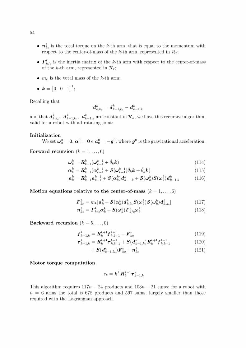
54

• n ℓkc is the total torque on the k-th arm, that is equal to the momentum with

respect to the center-of-mass of the k-th arm, represented in Rℓ;

• Γ ℓk/c is the inertia matrix of the k-th arm with respect to the center-of-mass

of the k-th arm, represented in Rℓ;

• mk is the total mass of the k-th arm;

• k =[0 0 1

]T;

Recalling thatdk

k,kc = dkk−1,kc − dk

k−1,k

and that dkk,kc , dk

k−1,kc , dkk−1,k are constant in Rk, we have this recursive algorithm,

valid for a robot with all rotating joint:

InitializationWe set ω0

0 = 0, α00 = 0 e a0

0 = −g0, where g0 is the gravitational acceleration.

Forward recursion (k = 1, . . . , 6)

ωkk = Rk

k−1(ωk−1k−1 + θkk) (114)

αkk = Rk

k−1(αk−1k−1 + S(ωk−1

k−1)θkk + θkk) (115)

akk = Rk

k−1ak−1k−1 + S(αk

k)dkk−1,k + S(ωk

k)S(ωkk)d

kk−1,k (116)

Motion equations relative to the center-of-mass (k = 1, . . . , 6)

F kkc = mk[a

kk + S(αk

k)dkk,kcS(ωk

k)S(ωkk)d

kk,kc ] (117)

nkkc = Γ k

k/cαkk + S(ωk

k)Γkk/cω

kk (118)

Backward recursion (k = 5, . . . , 0)

f kk−1,k = Rk+1

k f k+1k,k+1 + F k

kc (119)

τ kk−1,k = Rk+1

k τ k+1k,k+1 + S(dk

k−1,k)Rk+1k f k+1

k,k+1 (120)

+ S(dkk−1,kc)F

kkc + nk

kc (121)

Motor torque computation

τk = kTRk−1k τ k

k−1,k

This algorithm requires 117n − 24 products and 103n − 21 sums; for a robot withn = 6 arms the total is 678 products and 597 sums, largely smaller than thoserequired with the Lagrangian approach.

Bibliography

[1] S.H. Crandall, D.C.Karnopp, jr. E.F Kurtz, and D.C. Pridmore-Brown. Dynam-ics of mechanical and Electromechanical Systems. McGraw-Hill, 1968.

[2] J. Meisel. Principles of Electromechanical-Energy Conversion. Robert E. KriegerPublishing Company, 1984.

55

rigid body dynamics - polito

Documents