resonance in ac circuits. 3.1 introduction m m m h an example of resonance in the form of mechanical...

Resonance In AC Circuits

3.1 Introduction

MM

M

h

An example of resonance in the form of mechanical : oscillation

Potential energy change to kinetic energy than kinetic energy will change back to potential energy.

If there is no lost of energy cause by friction potential energy is equal to kinetic energy.

mgh = ½ mv ²It will oscillate for a long time.

Ep=mgh

Ek= ½ mv ²v

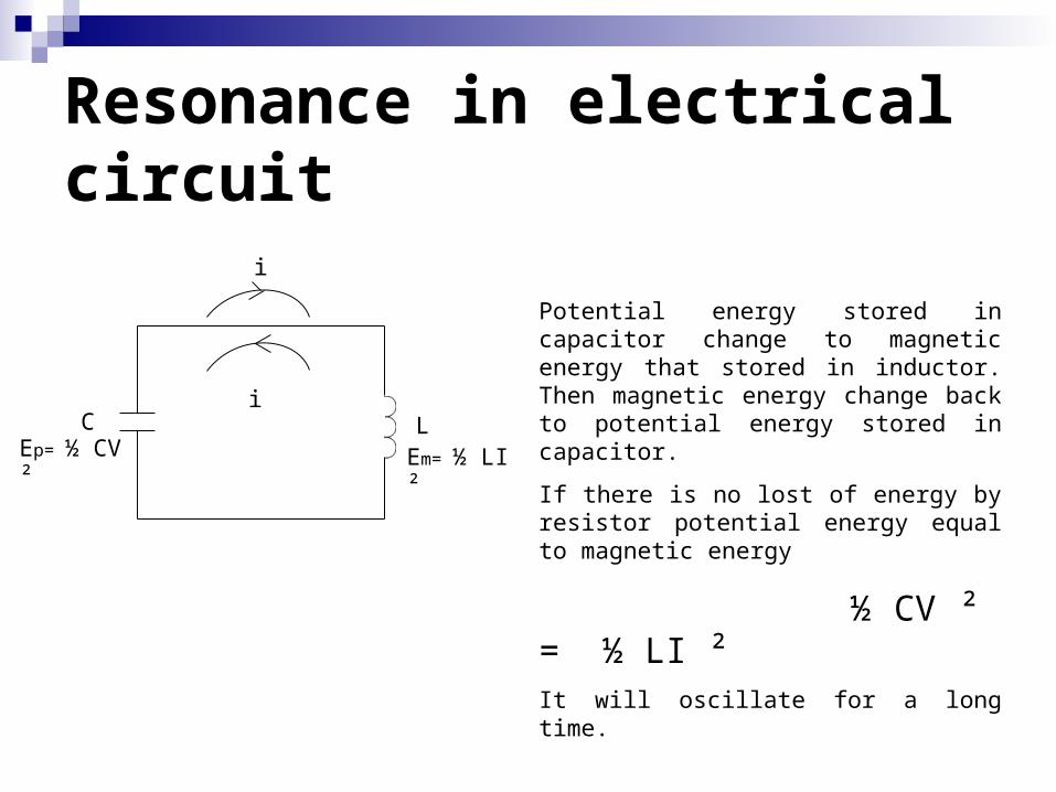
Resonance in electrical circuit

C L

i

i

Ep= ½ CV ² Em= ½ LI ²

Potential energy stored in capacitor change to magnetic energy that stored in inductor. Then magnetic energy change back to potential energy stored in capacitor.

If there is no lost of energy by resistor potential energy equal to magnetic energy

½ CV ² = ½ LI ²It will oscillate for a long time.

Characteristic of

resonance circuit

The frequency response of a circuit is maximum

The voltage Vs and current I are in phase

The impedances is purely resistive.

Power factor equal to one

Circuit reactance equal zero because capacitive and inductive are equal in magnitude

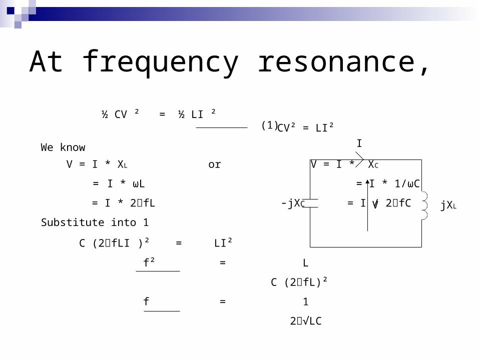
At frequency resonance,

(1)

V

I

jXL-jXC

CV² = LI²

We know

V = I * XL or V = I * XC

= I * ωL = I * 1/ωC

= I * 2חfL = I / 2חfC

Substitute into 1

C (2חfLI )² = LI²

f² = L

C (2חfL)²

f = 1

LC√ח2

½ CV ² = ½ LI ²

Ideal case ( no resistance)

Practical ( energy loss due to resistance)

i

i

t

t

Main objective we analysis resonance circuits to find five resonance parameters :

a) Resonance frequency, ωo

Angular frequency when value of current or voltage is maximum

b) Half power frequency, ω1 and ω2

Frequency where current (or voltage) equal Imax/√2 (or Vmax/√2 ).

c) Quality factor, Q Ratio of its resonant frequency to its bandwidth

d) Bandwidth, BW Difference between half power frequency

3.3 Series Resonance Circuits

R

VR VL

R j XL

- j XCV

By KVL : V = VR + VL + VC

= VR + jVL – jVC

At resonance XL = XC

Hence V = VR + 0

= VR

= IR * R

Vc

Figure 1

Series Resonance Circuits

R

VR VL

j XL

- j XCV Vc

Figure 1

Z = R + j XL - jXC

= R + j (XL – XC)

XL = 2πf L

XC = 1

2πf C

where

XL

R

XC f0

f

|Z|

(XL-XC)

f

f0

|I||Z|

|I| =|V|

|Z|

Resonance parameter for series circuita) Resonant frequency,ωo

The resonance condition is

ωoL = 1 / ωoC or ωo = 1 / √LC rad/s

since ωo = 2Пfo

fo = 1/ 2ח√LC Hz

b) Half power frequencies

At certain frequencies ω = ω1, ω2, the half power frequencies are obtain by setting Z = √2R

√ R² + (ωL – 1/ ωC)² = √ 2R

Solving for ω, we obtain

ω1 = - R/2L + √(R/2L)² + 1/LC rad/s

ω2 = R/2L + √(R/2L)² + 1/LC rad/s

Or in term of resonant parameter,

ω1 = ωo [ - 1/ 2Q + √ (1/ 2Q)² + 1 ] rad/s

ω2 = ωo [ 1/ 2Q + √ (1/ 2Q)² + 1 ] rad/s

c) Quality factor, Q

Ratio of its resonant frequency to its bandwidth.

Q = VL

VS

= [ I ] x XL

[ I ] x R

= ω L ; Q = XL

R R

fr Lח 2 = R

Q = VC

V

= [ I ] x XC

[ I ] x R = 1 ; Q = XC

ωC R R

= 1 fr CR ח2

or

d) Bandwidth, BW

BW = ω2 – ω1

= ωo [√ 1+ (1/ 2Q)² + 1/ 2Q ] - ωo [√ 1+ (1/ 2Q)² - 1/ 2Q ]

= ωo [ 1/ 2Q + 1/2Q ]

= ωo [2/ 2Q]

= ωo / Q

Q = ωoL /R = 1/ ωoCR

thus,

BW = R / L = ωo / Q

or, BW = ωo²CR

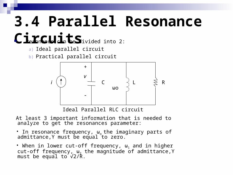
3.4 Parallel Resonance Circuits Resonance can be divided into 2:

a) Ideal parallel circuit

b) Practical parallel circuit

At least 3 important information that is needed to analyze to get the resonances parameter:

• In resonance frequency, ωo the imaginary parts of admittance,Y must be equal to zero.

• When in lower cut-off frequency, ω1 and in higher cut-off frequency, ω2 the magnitude of admittance,Y must be equal to √2/R.

i

+

v

-

RC L

Ideal Parallel RLC circuit

ωo

Resonance parameter for ideal RLC parallel circuit

R-jXc jXL

Ideal Parallel RLC circuitYT

Lc XXj

R

111YT =

)()(11

jBG

LCj

R

Whereas G(ω) is the real part called the conductance

and B(ω) is the imaginary parts called the susceptance.

a) Resonant frequency,ωo

Angular resonance frequency is when B(ω)=0.

b) Lower cut-off angular frequency, ω1

Produced when the imaginary parts = (-1/R)

sradLC

LC

/1

;01

210

LCRCRC

RLC

1

2

1

2

1

11

2

1

c) Higher cut-off angular frequency, ω2.

Produced when the imaginary parts = (1/R)

d) Quality Factor, Q

e) Bandwidth, BW

sradLCRCRC

RLC

/1

2

1

2

1

11

2

1

RCQ

L

CR

L

RQ

0

0

QRCBW 0

12

1

Duality ConceptDuality Concept

R

VR VL

j XL

- j XCV Vc

Figure 1

Series circuit Parallel circuit

i

+

v

-

RC L


Z = Z1 + Z2 + Z3

Z = R + j XL - jXC

Y = Y1 + Y2 + Y3

Y =

Lc XXj

R

111

LCj

R 11

Y Z = R + j (ωL – ) C1


R

VR VL

j XL

- j XCV Vc

Figure 1


i

+

v

-

RC L


LCj

R 11

Y Z = R + j (ωL – ) C

1

R R

1

L C

C L


R

VR VL

j XL

- j XCV Vc

Figure 1


i

+

v

-

RC L


ω1 = - R/2L + √((R/2L)² + 1/LC) rad/s

ω2 = R/2L + √((R/2L)² + 1/LC) rad/s

ω1 = - 1/2RC + √((1/2RC)² + 1/LC) rad/s

ω2 = 1/2RC + √((1/2RC)² + 1/LC) rad/s

Resonance parameter for practical RLC parallel circuit

Practical Parallel RLC circuit

i

+

V

-

R1

C

L

I1 IC

I1

IC

Z1 = R1 + jXL = |Z1|/θθ

|I1|cosθ

|I 1|sin

θ

I


Practical Parallel RLC circuit

i

+

V

-

R1

C

L

I1 IC

I1

IC

Resonance occur when |I1|sinθ = IC θ

|I1|cosθ

|I 1|sin

θ

I

Resonance occur when |I1|sinθ = IC

|I1|sinθ = IC

|V|

|Z1|x

XL

|Z1|

|V|=

XC

XL

|Z1|2=

XC

1

2πfrL

R2 + (2πfrL)2= 2πfrC

R2 + (2πfrL)2L

=C

(2πfrL)2 = LC

- R2

21

2

1

L

R

LCrf

Q factor

XL

R

2πfrL

=

=

Q = current magnification IC=|I1|sinθ

I=

|I1|cosθ

tanθ

=

R

I1

IC

θ

|I1|cosθ

|I 1|sin

θ



i

+

V

-

R1

C

L

Second approach to analyze this circuit is by changing the series RL to parallel RL circuit.

The purpose of this transformation is to make it much more easier to get the resonance parameter.

RL in series

Rl

L

Rl jXp

RL in parallel

ppT

l

ll

l

llllT

llT

jXRY

XXR

jR

jXRjXRY

jXRZ

11

1112222

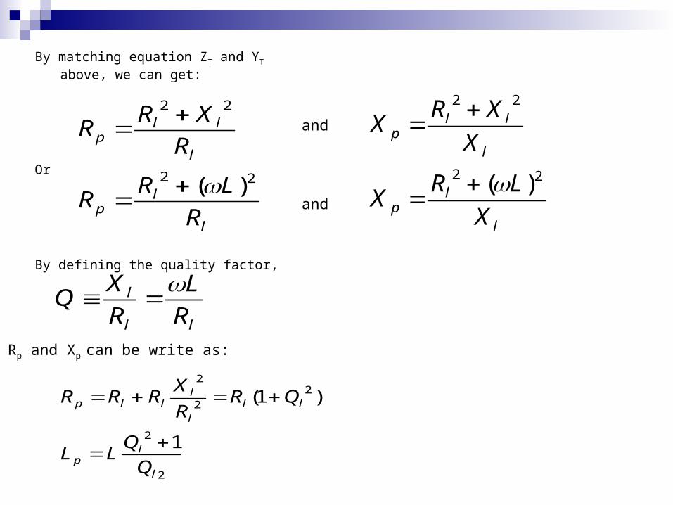
By matching equation ZT and YT above, we can get:

Or

By defining the quality factor,

l

lp

l

llp

R

LRR

R

XRR

22

22

)(

and

and

l

lp

l

llp

X

LRX

X

XRX

22

22

)(

ll

l

R

L

R

XQ

Rp and Xp can be write as:

2

2

2

2

2

1

)1(

l

lp

ll

l

lllp

Q

QLL

QRR

XRRR

Resonance parameter

a) Angular resonance frequency, ωo

b) Lower cut-off angular frequency, ω1


L

CR

LCX

R

LCl

l

l2

02

2

111

sradCLCRCR

RLC

ppp

/1

2

1

2

1

11

2

1

c) Higher cut-off angular frequency, ω2.

d) Quality Factor, Q

e) Bandwidth, BW


sradCLCRCR

RLC

ppp

/1

2

1

2

1

11

2

2

RCQ

L

CR

L

RQ

pp

p

QCRBW

p

012

1

resonance in ac circuits. 3.1 introduction m m m h an example of resonance in the form of mechanical...

Documents