Report No. 19377-RU

RussiaTargeting and the Longer-lerm Poor(In Two Volumes) Volume I1: Annexes

May 1999

Poverty Reduction and Economic Management (ECSPE) andHuman Development Networks (ECSHD)Europe and Central Asia Region

Document of the World Bank

Pub

lic D

iscl

osur

e A

utho

rized

Pub

lic D

iscl

osur

e A

utho

rized

Pub

lic D

iscl

osur

e A

utho

rized

Pub

lic D

iscl

osur

e A

utho

rized

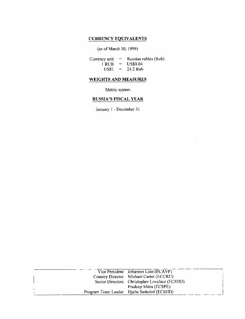
CURRENCY EQUIVALENTS

(as of March 30, 1999)

Currency unit = Russian rubles (Rub)I RUB = US$0.04US$1 = 24.2 Rub

WEIGHTS AND MEASURES

Metric system

RUSSIA'S FISCAL YEAR

January I - December 31

Vice President Johannes Linn (ECAVP)Country Director Michael Carter (ECCRU)Sector Directors Christopher Lovelace (ECSHD)

Pradeep Mitra (ECSPE)Program Team Leader Hjalte Sederlof (ECSHD)

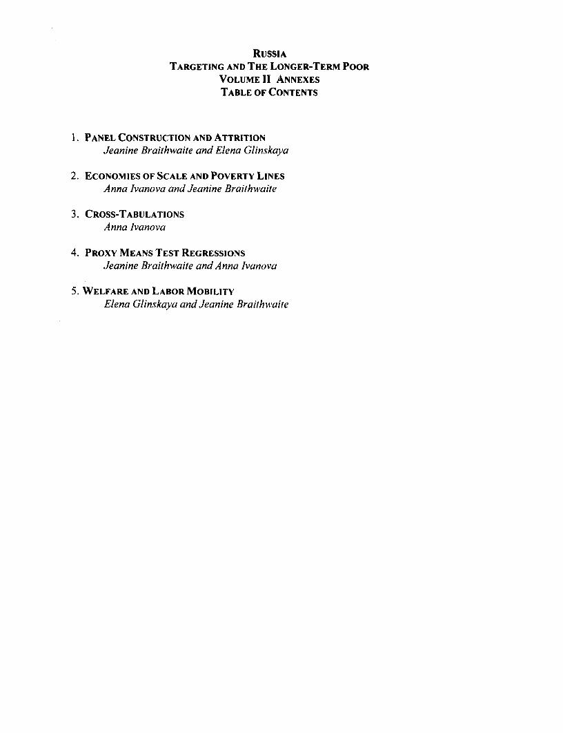
RUSSIATARGETING AND THE LONGER-TERM POOR

VOLUME II ANNEXES

TABLE OF CONTENTS

1. PANEL CONSTRUCTION AND ATTRITIONJeanine Braithwaite and Elena Glinskaya

2. ECONOMIES OF SCALE AND POVERTY LINESAnna Ivanova and Jeanine Braithwaile

3. CROSS-TABULATIONSAnna Ivanova

4. PROXY MEANS TEST REGRESSIONSJeanine Braithwaile and Anna Ivanova

5. WELFARE AND LABOR MOBILITY

Elena Glinskaya and Jeanine Braithwaite

ANNEX ONE

PANEL CONSTRUCTION & ATTRITION: RUSSIA 1994-96

JEANINE BRAITHWAITE (ECSPE)

1. The basic source of data for this report is a panel constructed from three rounds(waves) of the Russian Longitudinal Monitoring Survey (RLMS), which are publiclyavailable on the world wide web'. Households were matched to generate a panel of 2.675households for which data were available for each of the three years. Over the course ofthe three years, some households dropped out of the survey and others were added. Thepanel is constructed of households which were present in all three rounds and reportedenough information for their poverty status to be ascertained. There is a known danger ofbias owing to attrition, as households on the extremes of the distribution (i.e. the very richor the very poor) are more likely to drop out than others, although Glinskaya andBraithwaite (1997) found that attrition was not a significant issue for the RLMS panel(see below).

PANEL CONSTRUCTION

2. The primary motivation behind the construction of the panel data set is that it beuseable and accessible to scholars, analysts, and policy makers in Russia. Most scholarsand policy analysts are not that accustomed to working with large data sets on personalcomputers, and the data collection activities of Goskomstat Rossii are highly centralizedand dependent on main-frame computing time for processing.

3. In contrast, this study's panel dataset is made available as a public good (i.e. nocharges are required to obtain the data) for anyone who is interested in various definitionsof poverty and the poverty line. The original data set was made public by UNC on anInternet (World Wide Web) site, and this data set follows a similar the open accesspolicy (without being available on the web but happily supplied on diskette). So thatRussian scholars and policy analysts can quicklly open up a dataset and duplicate the mainfindings of this study, the following "short-cuts" were adopted.

The panel file is on the household level only. The individual files provided by UNCare extremely large and unwieldy. Interested parties can quickly match-merge theWorld Bank's version of the RLMS data set with the individual files by using theoriginal identification numbers found as "dupaid" "dupbid" and "dupcid".

The website is http://www.cpc.unc.edu/projects/rlms.

* Results and all cross-tabulations are run on only those households which are in thepanel every year, although cross-sectional data are available from UNC. Technicallyspeaking, this means that the World Bank version of the data runs some risk forattrition bias, which occurs as households drop out of a panel over time. Questions ofattrition are explored below.

* In the World Bank version of the RLMS data set, several variables have beenredefined, and the Bank poverty standard is based on household consumption, nothousehold income as in the UNC case. Since the household consumption variable isso significant, differences between the Bank and UNC are presented below. All of thevariables created by the Bank which are critical for the analysis, such as the definitionof the unemployed, disabled, and pensioners, are included in the panel file.

* The most important created variables are: total consumption, per capita consumption.per Goskomstat equivalent adult consumption, the cross-sectional poverty dummyvariables, and the poverty transition variable. For convenience, the study uses theseterns in the following way to characterize the various possible combinations ofpoverty status of the households over the three years as embodied in the povertytransition variable:

Longer-term poor: poor in every year (p-p-p)Never poor: not poor in every year (np-np-np)Escapedfrom poverty: poor in first year or first atnd second year, then not poor afterwards

(p-np-np or p-p-np)Fell into poverty. not poor in first year or first and second year, then poor afterwards (np-p-p,

np-np-p)Mixed: other patterns.

4. Additionally, exact patterns are indicated by symbols in the table column heading,with "p" designating poor and "np" for not poor. A notation such as p-np-np wouldrepresent escaping from poverty after the first year, while np-np-p would represent a fallinto poverty after the second year.

5. Poverty can be measured on either a household, individual, or population basis.Much basic poverty information is on an individual level, which is equivalent to tdepopulation as a whole if the sample is self-weighting. The RLMS sample is evaluatedvery positively by Heeringa (199?), in a report found on the RLMS Website.

6. UNC did include a vector of weights to be used when scaling up to the populationlevel, but these weights were found to have a negligible effect--cross-tabulations with andwithout the weights were equal to several decimal places, and standard tests failed todistinguish between outcomes with and without these weights. Therefore, the weightswere not further used in this analysis. However, attrition is potentially a more seriousproblem than inflating to the population level correctly, particularly since there is no clearway to remedy the problem (Deaton 1997).

2

7. Poverty in this study was based on a modified version of the consumption variableprovided by UNC in the data files.' The UNC( consumption variable was comprised ofpurchases of goods and services and the imputed value of food produced on the privateplot and consumed during the survey recall period. The imputation was based onpurchase prices collected in a community questionnaire. The modifications consistedprimarily of excluding savings and operations in foreign currency from the Bank'sdefinition of consumption. Household savings were non-existent or extremely low forpoor households and were overall quite low on average.

8. The poverty line used was a household-specific one, based on the officialsubsistence minimum calculated by Goskomstat Rossii. The subsistence minimum isdifferentiated for children, active-age adults, and adults at or past the statutory retirementage (60 for men, 55 for women), although it is usually published in a per capita form.The age-specific subsistence minimums were multiplied by the number of householdmembers in each category and summed to create a household-specific poverty threshold.This was then compared to the household's total consumption to determine whether thehousehold (and its constituent members) were poor or not. In this sense, our poverty lineincludes an embedded equivalence scale (Annex Two).

9. In the publicly-available data set, UNC provided additional poverty variables forregionally-differentiated subsistence minimum, but these were not used for the basicconclusions in this study. These LUNC poverty variables are aggregated for 8 regions ofRussia and are said to reflect differences in regional prices (Lokshin and Popkin 1998).However, they can not be used for this study as they are not equal to the actual legalsubsistence minimums in use in Russia during the study period (for comparison, theofficial statistics are presented in Annex Three).

10. First of all, the UNC variables do not correspond to the local subsistenceminimums used by some oblasts to allocate local social assistance or in 3 cases, the socialassistance pilot benefit. There are currently 89 such local subsistence minimums ascalculated by Goskomstat Rossii according to methodological instructions issued by theformer Ministry of Labor. There are additional regional variations as some areas (e.g.Moscow city and oblast) have chosen their own specific local standard. Second, in spiteof known considerable price variation in Russia, when checked previously for the 1994data, the 1995 World Bank poverty assessment found that there was essentially no majordifference in the overall headcount between comparing consumption to 89 individuallines instead of one national line. This is because although the cost of living undoubtedlyvaries across Russia, so do salaries and other sources of income, such that nominalconsumption levels tend to mirror price variation. While in principle it would be best torepeat this analysis on the panel data, it would require obtaining very detailed informationfrom Goskomstat Rossii on the 89 individual CPIs for the fieldwork period in each of

Technical detail on the consumption aggregate and other panel construction issues is provided in Annex One, while equivalence, thepoverty line, and sensitivity analysis are presented in Annex Two. For ease of exposition, only one poverty line is used in thebody of the study, the official prozhitochniy minimum (subsistence minimum).

3

three years, which are not routinely published, let alone the computational time to deflatethe data by oblast.

11. For example, but while the UNC consumption variable, correctly, did not includeexpenditures on the purchase of a house or apartment or of consumer durables such asautomobiles, it did include household expenditures on feed, seed, fertilizer, and otheritems used on the private plot. Typically, such expenditures are separated out from thehousehold's consumption, since thiey are investment for next period's consumption, andare handled through accounting for net profit from agricultural activities. However, giventhe timing of the fieldwork of the survey (during the Autumn of each year), this particularconcern about household expenditure on feed, seed, and other items used on a private plotis not a major problem for the analysis, since the vast majority of such expenditures occurin the Spring planting season, not the Fall harvest season.

12. One of the biggest problems in comparing poverty findings among differentstudies is that the choice of basis is quite significant for outcomes. Much of the UNCwork to date on its data set has been on a household reported income basis, but mosthousehold respondents in surveys in Russia and in other countries (including thedeveloped market economies) do not report accurately their income level. However,consumption which is drawn mainly from expenditure questions is much higher and morereliable than income in most transition and developing economy contexts, owing to thepervasive nature of the informal sector (Braithwaite 1995).

13. In the RLMS, there is a substantial degree of under-reporting of official income(Table A-1).

4

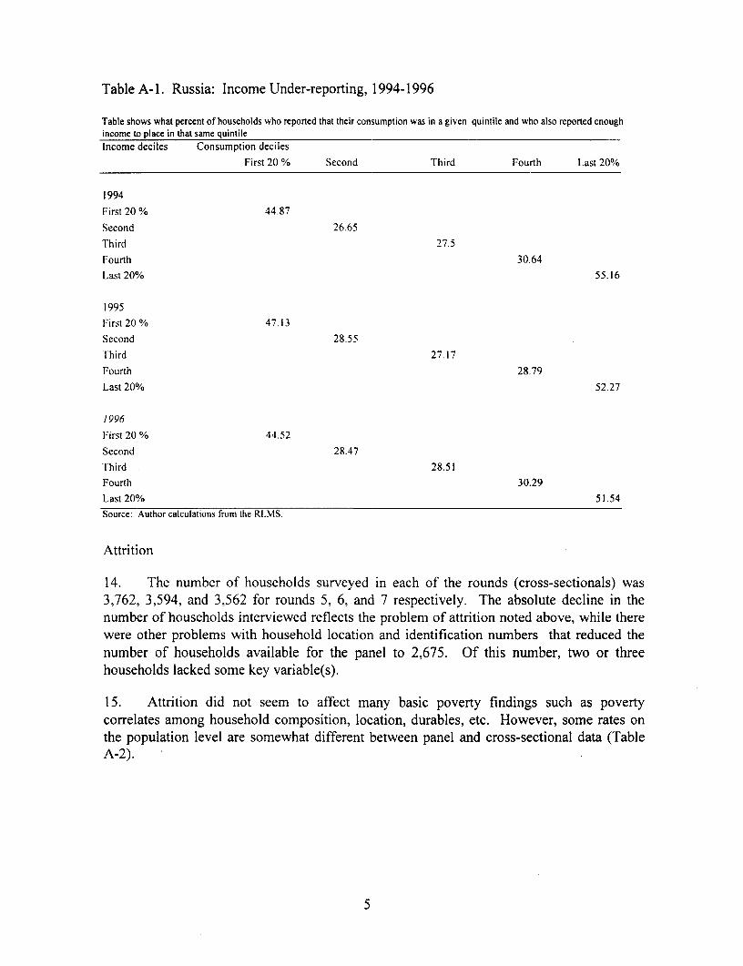
Table A-1. Russia: Income Under-reporting, 1994-1996

Table shows what percent of households who reported that their consumption was in a given quintile and who also reported enoughincome to place in that same quintileIncome deciles Consumption deciles

First 20 % Second Third Fourth Last 20%

1994

First 20 % 44.87

Second 26.65

T'hird 27.5

Fourth 30.64

Last 20% 55.16

1995

First 20 % 47.13

Second 28.55

'I'hird 27.17

Fourth 28.79

Last 20% 52.27

1996

First 20 % 44.52

Second 28.47

Third 28.51

Fourth 30.29

Last 20% 51.54Source: Author calculations from the RLMS.

Attrition

14. The number of households surveyed in each of the rounds (cross-sectionals) was3,762, 3,594, and 3,562 for rounds 5, 6, and 7 respectively. The absolute decline in thenumber of households interviewed reflects the problem of attrition noted above, while therewere other problems with household location and identification numbers that reduced thenumber of households available for the panel to 2,675. Of this number, two or threehouseholds lacked some key variable(s).

15. Attrition did not seem to affect many basic poverty findings such as povertycorrelates among household composition, location, durables, etc. However, some rates onthe population level are somewhat different between panel and cross-sectional data (TableA-2).

5

Table A-2. Russia: Unemployment and Disability Rates

Unemployed (not working, Individual (% of unemployed Household (% of households lhaving at least onedoes not receive a pension out of total population) unemployved out of all hIouseholds)and wants to work)

round Scross-sectional 9.5 23panel 8.8 21.6

round 6crnss-sectional 9.4 22.3pane! 8.7 21

round -cross-sectional 10.6 24.4panel 9.9 23.2

Disabled (receiving Individual (% of disabled out Househiold (% of hiouseholds having at least onedisability pension) of total population) disabled out of all htouseholds)

round 5cross-sectional 2.4 6.5panel 2.4. 6.6

round 6cross-sectional 2.5 6.5panel 2.6 7.2

round -cross-sectional 2.6 7.0panel 2.7 7.3

16. Some concerns can be raised in relation to the possible bias of the presentedresults due to the panel sample attrition. To test the robustness of our measures we ran aseries of binary probit estimations on the sub-samples of observations for variousdemographic groups. For example, to test the possible bias in the poverty assessment forthe pensioners on the panel data we ran a model with the dichotomous dependent variablewhich is equal to one for the pensioners who stay in the panel through last three rounds ofthe survey and is equal to zero for the pensioners who fall out of the sample. Asexplanatory variables we use the polynomial of the log of the total householdexpenditure for the last round of the survey and the log of household size. Thepolynomial form of the household expenditure allows to capture possible non-linearity inattrition bias. Similar estimations are run for the other demographic groups of interest.The results of binary probit estimations are presented in Table A-3.

6

Table A-3: Russia: Binary probit estimation of the possible attrition bias. World BankPanel 1994-1996.

Families of Nuclear Single parent All familiespensioners families familiesCoefficient Coefficient Coefficient Coefficient

(St.Err) (St.Err) (St.Err) (St.Err)Log of household -6.6632 1.9166 -2.0463 .37386expenditure (4.6544) (3.6851) (8.0815) (1.3461)(LHHE)LHHE squared 0.9480 -0.18006 0.3363 -0.0149

(0.6166) (0.4345) (1.0294) (0.1642)LHHE cubed -0.04359 0.00523 -0.0165 -.0009

(0.0269) (0.0168) (0.04314) (0.0066)Log of household -0.1785 0.5652* -.01655 -0.4392***size (0.1684) (0.2370) (.04313) (0.0469)Constant 16.2817 -6.5589 3.6074 -0.6089

(11.5896) (10.3161) (20.8081) (3.6421)Prob>P2 0.2871 0.0707* 0.7407 0.000

* Significant with 90% probability** Significant with 95% probability**"Significant with 99.5% probability

17. The main conclusion is that attrition bias does not have a significant effect on thepoverty assessment results conducted on the panel sample verses the cross-sectionalsample (the coefficients on the total household expenditure variables are insignificant forall demographic groups and they are jointly insignificant also). However, there is apossibility for larger households to exit out of the panel sample disproportionately (thecoefficient for the family size is significant for the nuclear families and for all Russiasample). Disproportionate exit could lead to bias in the poverty findings for largerhouseholds.

Table A-4. Russia: Binary probit estimation of the possible attrition bias. World BankPanel 1994-1996.

Major Metropolitan Other urban Rural

Coefficient (St.Err) Coefficient (St.Err) Coefficient (St.Err)

Log of household expenditure -8.784 2.595(***) -7.037(**)(LHHE) (20.030) (4.714) (7.900)LHHE squared 0.602 -0.157(***) 0.564(**)

(1.389) (0.347) (0.590)LHHE cubed -0.014 0.003(***) -0.015(**)

(0.032) (0.008) (0.015)Log of household size -0.457*** 0.344*** -0.827***

(0.173) (0.059) (0.097)Constant 43.075 -12.578 29.833

(96.038) (21.269) (35.113)Prob>?2 0.0285*** 0.0000*** 0.0000***

* Significant with 90% probability; " Significant with 95% probability;" Significant with 99.5% probability; (),("),("') Jointly significant

7

18. Possible attrition bias in shown in the probit estimation by location of householdresidence (Table A-4). In all three locations, larger families are less likely to stay in thepanel sample. Total household expenditure does not have any significant effect on theprobability of being in the sample for households from metropolitan areas of Russia, butthe joint significance of the total household expenditure polynomial coefficients in otherurban areas of Russia and in the rural areas indicate a possible bias in poverty results forthese locations.

19. The negative combined coefficient on the total household expenditure variablesfor rural Russia implies that the poor rural Russian households are more likely to stay inthe panel sample and thus the poverty metrics will be biased toward zero for thesehouseholds, i.e., the poverty rate of rural households can be overestimated if the analysisis done solely on the panel sample. The positive coefficient on the other urban areas ofRussia expenditure indicate on the opposite picture. For this category we can expect toobserve a positive bias in the poverty measurements, or that the poverty rate of otherurban areas can be underestimated in comparison with the rate calculated on the cross-sectional sample. We do not observe any biases for the major metropolitan areas ofRussia based on the total household expenditure.

20. We also tested for attrition in a general, dynamic sense, starting from the initialpoverty status of the household. There seems to be no major differences in probabilitiesof exiting by the initial poverty status. 29 percent of the household which were initiallynon-poor exited, and 32 percent of the poor households exited. However, there are somedifferences in probability of attrition for the households of different characteristics. Thereare also seems to be differences in probabilities of leaving the sample for the same typesof households, but with the different poverty status.

21. Households headed by more educated individuals are more likely to exit thesample. This is true both for the households which were initially classified as poor and aswell as for the non-poor. Households headed by the young individuals which were abovethe poverty line in 1994 were more likely to exit than non-poor households headed by theolder individuals Households residing in the major Metropolitan areas are more likely tobe lost from the sample over time.

22. Poor female-headed households have a higher probability of exiting than non-poorfemale-headed households. Another substantial difference is the probability of exiting forpoor and non-poor households headed by the older heads.

23. Attrition is modeled below, and the Mills ratio for observing a household in thesample is included in the estimated equation. Sample weights were used in allregressions. The following computer output contains an estimation of equations relating"exit from the RLMS sample" to the set of family characteristics and to the indicators ofthe position in the distribution of expenditure in 1994. The first equation combines allobservations together, and includes controls for 5 initial expenditure quintiles.

8

Ie_pcq lowestIejpcq2Iejpcq3lepcq4le_pcq_5 highest, omitted.

The second and third equations are estimated for the "initially poor" household and "initially non-poor"households, respectively. By comparing the effect of the household characteristics on the exitprobabilities of poop and non-poor households one can say whether these characteristics have differentialeffects on the probabilities of exiting the sample.

gen not_att=0 if site5=.(924 missing values generated)

replace not_att= I if flag= = I&not_att=.(2675 real changes made)

tab not_att

not_att I Freq. Percent Cum.+-

0 l 1113 29.38 29.38 exited the sample during r6 or r7I 1 2675 70.62 100.00 stayed in the sample all 3 rounds

-- Total 1 3788 100.00

xi: dprobit not att ncatl 5 ncat2 5 ncat4 5 ncat5 5 ncat6 5 fh 5 rmh 5 rfh 5> yh_5 own_aut5 hhw_han5 hhw_mat5 hhw_une5 i.hhh_agg5 i.hhh_edg5 reg2 r• eg3 reg4 reg5 reg6 reg7 reg8 i.settl_t i.e_pcqu_5 if hhh_edg5-=0i.hhh_agg5 Ihhh _ 0-10 (naturally coded; Ihhh _ 0 omitted)i.hhh_edg5 Ihhh_e_0-3 (naturally coded; Ihhh_e_0 omitted)i.settl_t Isettl_1-3 (naturally coded; Isettl_1 omitted)i.e_pcqu_5 Ie_pcq_0-4 (naturally coded; Ie_pcq_o omitted)

Note: lhhh__10 dropped due to collinearity.Note: Ihhh_e_3 dropped due to collinearity.Iteration 0: Log Likelihood =-2255.0199Iteration 1: Log Likelihood = -2113.169Iteration 2: Log Likelihood =-2112.2748Iteration 3: Log Likelihood =-2112.2746

Note: Ihhh__10 dropped due to collinearity.Note: lhhh_e_3 dropped due to collinearity.

Probit Estimates Number of obs = 3727chi2(36) = 285.49Prob > chi2 = 0.0000

Log Likelihood = -2112.2746 Pseudo R2 = 0.0633

9

not att I dF/dx Std. Err. z P>Iz| x-bar [ 95% C.I. I

ncatl_5 .0281302 .0174688 1.61 0.107 .265629 -.006108 .062368

ncat2_5 .0436285 .012496 3.49 0.000 .498256 .019137 .06812

ncat4_5 .0340686 .0174789 1.95 0.051 .772471 -.000189 .068327

ncat5s5*1 .0130514 .035486 0.36 0.715 .1685 -. 0565 .082603ncat6_5 1 .0573945 .0195744 2.93 0.003 .434398 .019029 .09576

fh_5*| -.0164619 .0264056 -0.63 0.529 .108935 -.068216 .035292

rmh_5*| -. 0177607 .0709388 -0.25 0.800 .115106 -.156798 .121277

rfh_S*| -.0258643 .0562448 -0.47 0.640 .116716 -. 136102 .084374yh_5*1 -.2315659 .3013173 -0.81 0.418 .000805 -.822137 .359005

own_aut5*1 .0031446 .0197277 0.16 0.874 .21626 -.035521 .04181

hhw_han5 | -.0349653 .0354063 -0.99 0.323 .042662 -. 10436 .03443

hhw_mat5*| -. 0091224 .0384744 -0.24 0.811 .048565 -. 084531 .066286hhw_une5 | -. 0350801 .0222528 -1.58 0.115 .111081 -. 078695 .008535Ihhh_1*| -.1712426 .0766605 -2.37 0.018 .050443 -.321494 -.020991

Ihhh _2*1 -.2087467 .0742416 -2.97 0.003 .077542 -.354258 -.063236

Ihhh _3*1 -.1318319 .0701283 -1.98 0.048 .117789 -.269281 .005617Ihhh 4*1 -.1232551 .0698199 -1.85 0.064 .126375 -. 2601 .013589Ihhhs5*| -.0697493 .067135 -1.08 0.282 .121545 -.201331 .061833

Ihhh _6*1 -.087102 .0680868 -1.33 0.182 .104105 -. 22055 .046346Ihhh__7*l -.0700772 .0677408 -1.07 0.283 .088275 -. 202847 .062692Ihhh 8*| -.0357966 .0519611 -0.70 0.482 .110276 -.137638 .066045

Ihhh_e_l*l .0667591 .021547 3.09 0.002 .494231 .024528 .10899

Ihhh_e_2*1 .069058 .0209942 3.20 0.001 .317682 .02791 .110206

reg2*1 -.0336974 .1015481 -0.34 0.734 .066541 -.232728 .165333

reg3*1 .0242128 .0921604 0.26 0.796 .14784 -.156418 .204844

reg4*i .050412 .0888046 0.55 0.583 .178964 -.123642 .224466

reg5*1 -.0654049 .1019653 -0.66 0.507 .117252 -.265253 .134444

reg6*1 .0123302 .0935978 0.13 0.896 .14462 -.171118 .195779

reg7*1 -. 0357135 .1001856 -0.36 0.716 .099007 -.232074 .160647

reg8*1 -.107224 .1065108 -1.06 0.291 .096324 -.315981 .101533

Isettl_2*1 .1384914 .0989762 1.42 0.155 .62007 -.055498 .332481

Isettl 3*l .2446968 .063901 3.10 0.002 .239335 .119453 .36994

Ie_pcq_1*l .0216814 .0236354 0.91 0.365 .200698 -.024643 .068006

Ie_pcq 2*| .0451376 .0231442 1.90 0.058 .201503 -.000224 .090499

Ie_pcq_3*1 .0389958 .0237273 1.61 0.108 .199893 -. 007509 .0855Ie_pcq_4*1 .0243009 .0249272 0.96 0.336 .199624 -. 024556 .073157---------- +- _ _ _ _ _ _ _ _ _ _ _ _ _ _ _ _ _-_-_-_-_-_-_-_-__ -_-_-_-_-_-_ -_

obs. P I .7067346pred. P .7192291 (at x-bar)

(*) dF,/dx is for discrete change of dummy variable from 0 to 1

z and P>Iz| are the test of the underlying coefficient being 0

test Ihhh_ lIhhh_2 lhhh_3 lhhh_4 lhhh_5 lhhh_6 lhhh7 lhhh_8

( 1) Ihhh_1 = 0.0( 2) Ihhh_2 = 0.0( 3) Ihhh_3 = 0.0( 4) Tihh_4 = 0.0( 5) Ihhh_S = 0.0( 6) Ihhh_6 = 0.0

10

( 7) Ihhh_7 =0.0( 8) Ihhh_8 =. 0.0

chi2( 8) = 23.59Prob > chi2 = 0.0027

test Ihhh_e_1 Ihhh_e_2

(1) Ihhh e1 = 0.0(2) Ihhh_e_2 = 0.0

chi2( 2) = 12.00Prob > chi2 = 0.0025

test Isettl_2 Isettl_3

(1) Isettl 2 = 0.02) Isettl_3 = 0.0

chi2( 2) = 64.41Prob > chi2 = 0.0000

test le_cc_l lejcq2 le_pcq3 le_pcq4

( 1) le_pcq_l = 0.0( 2) le_pcqc2 = 0.0( 3) le_pcq_3 = 0.0( 4) le_pcq_4 = 0.0

chi2( 4) = 4.31Prob > chi2 = 0.3653

xi: dprobit not_att ncatl_5 ncat2_5 ncat4_5 ncat5_5 ncat6_5 fh_5 rmh_5 rfh_5> yh_5 own_aut5 hhw_han5 hhw_mat5 hhw_uneS i.hhh_agg5 i.hhh_edg5 reg2 r> eg3 reg4 reg5 reg6 reg7 reg8 i.settl_t if hhh_edg5-=0& r_pind_5==1i.hhh agg5 Ihhh _ 0-10 (naturally coded; Ihhh _ 0 omitted)i.hhh_edg5 Ihhh_e_0-3 (naturally coded; Ihhh_e_0 omitted)i.settl_t Isettl_1-3 (naturally coded; Isettl_l omitted)

Note: yh5 - = 0 predicts failure perfectlyyh_5 dropped and 1 obs not used

Note: Ihhh__10 dropped due to collinearity.Note: Ihhh_e_3 dropped due to collinearity.Iteration 0: Log Likelihood =-358.12005Iteration 1: Log Likelihood =-334.51312Iteration 2: Log Likelihood =-334.29195Iteration 3: Log Likelihood =-334.29185

Note: yh5 = 0 predicts failure perfectlyyh_5 dropped and 1 obs not used

11

Note: Ihhh 10 dropped due to collinearity.Note: Ihhh_e_3 dropped due to collinearity.

Probit Estimates Number of obs = 577

chi2(31) = 47.66Prob > chi2 = 0.0284

Log Likelihood = -334.29185 Pseudo R2 = 0.0665

not_att I dF/dx Std. Err. z P>|z| x-bar [ 95% C.I. I

ncatl_5 .0170982 .0367277 0.47 0.642 .415945 -.054887 .089083ncat2_5 .0535068 .0280989 1.90 0.057 .644714 -.001566 .10858ncat4_5 .0609713 .0443521 1.37 0.169 .923744 -.025957 .1479

ncat5_5*| -.0585799 .1280542 -0.47 0.637 .051993 -.309562 .192402ncat6_5 1 .0545006 .0513708 1.06 0.289 .265165 -.046184 .155185

fh_5*1 -.0249752 .0619239 -0.41 0.683 .145581 -. 146344 .096393rmh_5*1 .0425287 .255086 0.16 0.872 .020797 -. 457431 .542488rfh_5*| .0394317 .1862785 0.20 0.838 .041594 -.325667 .404531

own_aut5*| .0370645 .055817 0.65 0.516 .149047 -. 072335 .146464

hhw_han5*| -.0790592 .0951647 -0.86 0.388 .05026 -.265579 .10746hhw mat5*1 .0084355 .0897712 0.09 0.926 .062392 -.167513 .184384hhw une5 s -.0232185 .0412122 -0.56 0.573 .230503 -.103993 .057556Ihhh_1*| .0820122 .2078787 0.36 0.715 .055459 -.325423 .489447Ihhh 2*1 -.0352545 .2423915 -0.15 0.882 .079723 -.510333 .439824Ihhh _3*1 .0150194 .2243084 0.07 0.947 .169844 -. 424617 .454656

Ihhh _4*1 -.0649611 .2416711 -0.28 0.783 .166378 -.538628 .408706Ihhh _5*l .0321429 .2184743 0.14 C.885 .176776 -. 396059 .460345Ihhh _6*| -. 0520599 .2403586 -0.22 0.824 .109185 -. 523154 .419034Ihhh _7*1 .0260435 .2210253 0.12 0.908 .095321 -.407158 .459245Ihhh _8*j .0211726 .2024045 0.10 0.918 .097054 -.375533 .417878Ihhh e_1*1 .0703811 .0677988 1.04 0.298 .542461 -.062502 .203264Ihhh e 2*| .0663722 .0673291 0.97 0.333 .348354 -.06559 .198335

reg2*1 .2600568 .0981407 1.54 0.124 .067591 .067705 .452409reg3*1 .2901258 .1156535 1.65 0.099 .15078 .063449 .516802reg4*| .295624 .1257071 1.64 0.101 .183709 .049243 .542005reg5*1 .2046427 .1547241 1.04 0.297 .133449 -.098611 .507896reg6*1 .2139176 .1491098 1.11 0.267 .133449 -.078332 .506167reg7*1 .2677949 .1127825 1.53 0.126 .114385 .046745 .488845reg8*1 .188076 .1617602 0.95 0.344 .131716 -.128968 .50512

Isett:L_2*1 -.2524389 .2019789 -1.13 0.258 .636049 -.64831 .143432Isett:L.3*1 -.0740639 .2455282 -0.31 0.759 .285962 -.55529 .407162

_-----+- __-_ -_

obs. P .6880416pred P .7017272 (at x-bar)

(*) dF/dx is for discrete change of dummy variable from 0 to 1z and P>|z| are the test of the underlying coefficient being 0

test Ihhhl lIhhh_2 lhhh_3 lhhh_4 lhhh_5 lhhh_6 Ihhh_7 lhhh_8

(1) Ihh:h_I = 0.0(2) Ihhh_2 = 0.0

12

(3) lhhh_3 = 0.0(4) Ihhh_4 = 0.0(5) Ihhh_5 = 0.0(6) Ihhh_6 = 0.0(7) Ihhh7 = 0.0(8) Ihhh_8 =0.0

chi2( 8) = 4.31Prob > chi2 = 0.8282

test Ihhh_e I lhhh_e_2

( 1) Ihhh_e 1I= 0.0( 2) Ihhh_e_2 = 0.0

chi2( 2) = 1.14Prob > chi2 = 0.5647

test Isettl_2 Isettl 3

(1) Isettl 2 = 0.0( 2) Isettl3 = 0.0

chi2( 2) = 15.83Prob > chi2 = 0.0004

xi: dprobit not_att ncatl_5 ncat2_5 ncat4_5 ncat5_5 ncat6_5 fh_5 rmh_5 rfh_5• yh_5 own_aut5 hhw_han5 hhw_mat5 hhw_une5 i.hhh_agg5 i.hhh_edg5 reg2 r• eg3 reg4 reg5 reg6 reg7 reg8 i.settl t if hhh_edg5 =0& r_pind_5 = =0i.hhh_agg5 Ihhh__0-10 (naturally coded; Ihhh_0 omitted)i.hhh_edg5 Ihhh_e_0-3 (naturally coded; Ihhh_e_0 omitted)i.settl_t Isettl_1-3 (naturally coded; Isettl_l omitted)Note: Ihhh_1 dropped due to collinearity.Note: Ihhh e_3 dropped due to collinearity.Iteration 0: Log Likelihood =-1895.0911Iteration 1: Log Likelihood =-1768.0141Iteration 2: Log Likelihood =-1767.2188Iteration 3: Log Likelihood =-1767.2183Iteration 4: Log Likelihood =-1767.2183

Note: Ihhh__1 dropped due to collinearity.Note: Ihhh_e_3 dropped due to collinearity.

Probit Estimates Number of obs = 3149chi2(32) = 255.75

Prob > chi2 = 0.0000Log Likelihood = -1767.2183 Pseudo R2 = 0.0675

13

not_at I dF/dx Std. Err. z P> Izl x-bar 1 95% C.]. ]-+-

ncatl_5 .0301684 .0200911 1.50 0.133 .238171 -.009209 .069546

ncat2_5 .0400104 .0139064 2.88 0.004 .471261 .012754 .067267

ncat4_5 .0305927 .0191174 1.60 0.110 .744998 -.006877 .068062ncat5_5*l .0177325 .0372565 0.47 0.638 .189902 -.055289 .090754

ncat6_5 1 .0539298 .0210748 2.56 0.011 .465545 .012624 .095236

fh_5*l -. 0136439 .029495 -0.47 0.641 .102255 -. 071453 .044165rmh_5*1 -. 040258 .0756657 -0.54 0.586 .132423 -. 18856 .108044rfh_5*1 -. 0443435 .0601473 -0.76 0.450 .130518 -. 16223 .073543

yh_5*| -. 0365139 .3151737 -0.12 0.905 .000635 -. 654243 .581215

own aut5*F -. 0014127 .0207368 -0.07 0.946 .228644 -. 042056 .039231

hhw_hanS | -. 0243688 .0389283 -0.63 0.531 .041283 -. 100667 .051929hhw_mat5*1 -. 0164092 .0433851 -0.38 0.702 .046046 -. 101442 .068624hhw_une5 | -. 0421987 .0270048 -1.56 0.118 .089235 -. 095127 .01073

Ihhh _ 2*1 -.0123106 .0465736 -0.27 0.790 .077167 -.103593 .078972

Ihhh_3*1 .0496348 .040697 1.17 0.242 .108288 -. 03013 .1294

Ihhh 4*1 .075145 .0391655 1.80 0.073 .119085 -. 001618 .151908

Ihhh 5*| .1091874 .0363206 2.69 0.007 .111464 .038 .180374

Ihhh_6*1 .1070025 .0358366 2.67 0.008 .103207 .036764 .177241

Ihhh _ 7*1 .1082029 .0360918 2.66 0.008 .087012 .037464 .178942

Ihhh _8*| .1418214 .0352298 3.42 0.001 .112734 .072772 .210871

Ihhh 10*| .1790614 .0536257 2.90 0.004 .23182 .073957 .284166

Ihhh_e_l*t .0659228 .0227391 2.89 0.004 .485233 .021355 .110491

Ihhh e_2*1 .0694923 .0221721 3.05 0.002 .312163 .026036 .112949

reg2*1 -.147173 .1321318 -1.18 0.237 .06637 -.406146 .111801

reg3*1 -.0766818 .1217563 -0.65 0.514 .147348 -. 31532 .161956reg4*1 -. 0405291 .1170329 -0.35 0.724 .178152 -. 269909 .188851

reg5*1 -. 1544854 .1287401 -1.27 0.205 .114322 -. 406811 .09784reg6*1 -. 066323 .1209705 -0.57 0.571 .146713 -. 303421 .170775reg7*1 -.1485605 .130091 -1.21 0.227 .095903 -. 403534 .106413reg8*1 -.2025745 .1325936 -1.62 0.106 .08987 -. 462453 .057304

Isettl_2*1 .2383255 .1174667 2.05 0.040 .617021 .008095 .468556Isettl_3*1 .2964198 .0639022 3.39 0.001 .230867 .171174 .421666

---+-

obs. P I .7103842pred. P I .723671 (at x-bar)

(*) dF/dx is for discrete change of dummy variable from 0 to Iz and P> IzI are the test of the underlying coefficient being 0

test Ihhh_I Ihhh_2 lhhh_3 Ihhh_4 lhhh_5 lhhh_6 lhhh_7 lhhh_8

( 1) Ihhh_10 = 0.0(2) Ihhh_2 = 0.0(3) Ihhh_3 = 0.0(4) Ihhh_4 = 0.0(5) hbh_h5 = 0.0(6) Dhhh_6 = 0.0(7) Ihhh_7 = 0.0(8) hhh_ 8 = 0.0

chi2( 8) = 28.10

14

Prob > chi2 = 0.0005

test lhhh_e_1 Ihhh_e_2

(1) Ihhh e_1 = 0.0(2) Ihhh_e_2 = 0.0

chi2( 2) = 10.85Prob > chi2 = 0.0044

test Isettl_2 Isettl_3

(1) Isettl 2 = 0.0(2) Isettl 3 = 0.0

chi2( 2) = 51.23Prob > chi2 = 0.0000

log close

LABELSncatl_S # of small children in the hhncat2_5 # of 7-18 y.old children in the hh

# of 19-60 males in the hh omittedncat4_5 # of 19-55 females in the hhncat5_5 retired malesncat6 5 retired females

th 5 female headed hhrmh 5 retired female headed hhrth_5 retired female headed hhyh_5 young person headed hh

own aut5 = 1 if own autohhw han5 = I if handicaps in the hhhhw mat5 = I if a member on maternity leavehhw_une5 = I if a member is unemployed

hh head age groupIhhh_1 18-23Ihhh_2 24-29Ihhh_3 29-34Ihhh_4 35-39Ihhh_5 40-44Ihhh_6 45-49Ihhh_7 50-55Ihhhh_8 56-60

older then 60 omittedhh head education group

Ihhh_e_l ptu or lowerIhhh_e_2 technicum

university omittedregions, Moscow and St. Petersburg omitted

reg2

15

reg3reg4reg5reg6reg7reg8

Isettl_2Isettl_3Ie_pcq_1 lowest pc expenditure quintileIe_pcq_2le_pcq_3Ie_pcq_4

********* * *****

thie following is what I had written up:

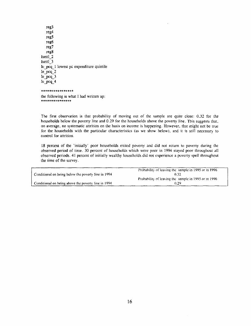
The first observation is that probability of moving out of the sample are quite close: 0.32 for thehouseholds below the poverty line and 0.29 for the households above the poverty line. This suggests that,on average, no systematic attrition on the basis on income is happening. However, that might not be truefor the households with the particular characteristics (as we show below), and it is still necessary tocontrol for attrition.

18 percent of the 'initially' poor households exited poverty and did not return to poverty during theobserved period of time. 30 percent of households which were poor in 1994 stayed poor throughout allobserved periods. 41 percent of initially wealthy households did not experience a poverty spell throughoutthe time of the survey.

Probability ot leaving the sample in 1995 or in 1996Conditional on being below the poverty line in 1994 0.32

Probability ot leaving the sample in 1995 or in 1996Conditional on being above the poverty line in 1994 0.29

16

Annex Two

Economies of Scale & Poverty Lines: Russia 1994-96

ANNA IVANOVA (U.WISC.)JEANINE BRAITHWAITE (ECSPE)

I. The purpose of this annex is to lay out the most important issues on economies ofscale and the poverty line, since these two parameters are critical for our povertyconclusions. For our poverty and inequality analysis an important question was toidentify resources available to each household member taking into account possibleeffects of economies of scale and the composition of the household. It is extremelydifficult to answer this question without reliable data on the distribution of individualconsumption within the household (information which shows whether one householdmember such as an active-age male consumes more food and other goods than otherhousehold members such as children). This is sometimes called the "unitary household"problem, and results from the extreme difficulty of collecting (or observing) reliableinformation about individuals, especially children. It is possible to approximate resourcesavailable to individual household members when making certain assumptions about theallocation of resources within the household. There are three approaches which haveoften been used: the Engels curve method, the Rothbart approach, and using informationabout subjective perceptions of poverty.

2. Under all the approaches, we can assume that each member consumes an equalportion of available resources and that there are some economies of size in householdconsumption (resulting from the presence of public goods). Economies of size inhousehold consumption mean that the marginal increment to total household expendituresof an additional household member declines with each subsequent. In more prosaicterms, the idea is that a large family can "stretch" a stew to feed one more by addingpotatoes instead of meat, children can wear hand-me-downs, and that the total cost of rentand utilities is either fixed or varies little with an additional person, so that the marginalcost of the additional person is lower (because the average cost is the total cost divided byan increasing number of members).

3. Besides this effect of size, there are the questions of equivalence mentioned in thefirst paragraph. Equivalence in this sense means determining what fraction of theconsumption of one household member (usually taken as an adult male for convenience)is covered by the consumption of other members. For example, one could expect thatchildren would consume less food than parents, and that an employed woman would havemore expenditures on professional clothing, transportation, and meals consumed outsidethe home than a retired grandmother also living in the household. In this case, thechildren and the pensioner would have lower consumption than the adult female in this

household, and their consumption could be said to be equivalent to (for example) 50 and70 percent respectively of the adult female's consumption. Although in principle weagree with the idea that all household members do not consume exactly identical amountsof total household consumption, particularly in developed market economies, we are lessconvinced about the extent of equivalence in many transition economies.

4. There are several factual observations about relative prices and actual payments intransition economies, as well as cultural specifics, which raise questions as to the actual(as opposed to theoretical) extent of equivalence in household consumption in transitioneconomies. Armenia provides a good illustration of these considerations. When Armeniafirst began its economic reform program with the World Bank in 1994. no one paid anyrmoney period for rent or utility payments even though these fixed prices were essentiallyzero when compared to the hyperinflated prices of food. The rent and utility paymentcollection systems had broken down during the armed conflict with Azerbaijan (1992-94)and the country was almost completely blockaded from land or rail freight, and theairport needed reconstruction before it could handle significant air freight. Thepopulation was subsisting almost exclusively on international and private humanitarianassistance (World Bank 1996).

5. However, at that time, neither the international non-governmental organizationsnor the World Bank could find any indication of widespread or even pockets of grosschild malnutrition (wasting), and little indication of prolonged child malnutrition(stunting). How could this be? The answer is found in Armenian cultural values, whichput children above all others in the family and society. Grandparents were semi-starvingthemselves in order to give food to their grandchildren and parents were also restrictingtheir intake. CARE documented significant and widespread weight loss among theArmenian elderly.

6. In such a situation, the standard OECD assumption that equivalence for childrenis 50 percent of adult consumption, and for the elderly, 70 percent, is clearly wrong. Inthe Armenian case in these terrible years, children were consuming at least 100 percent ofadult consumption, and the elderly were consuming imluch less, arguably under 50 percentof adult consumption. Unfortunately, it is extremely dit'ficult to measure what actualindividual equivalence is in general, and certainly not in the Armenian case given thevery limited survey information available.

7. Furthermore, it is quite difficult to argue that there were significant economies ofsize in consumption in Armenia from declining marginal contribution of a householdmember to average cost of rent and utilities, since hardly anyone paid any rent or utilitybills during this period. Even for the cost of heating it would be difficult to positeconomies of size, since the usual practice for a group of families living in an apartmentbuilding was to rotate heating responsibilities in the following way. Seriatim, familieswould purchase coal or wood and heat one room of their flat, in which every other personin the building could sit in the semi-heated semi-darkness. The formula for cost sharing

2

was rotation, or to think of it in another way, a flat fee per household which was invariantto the number of household members.

8. Fortunately, the government's economic reform program was successful, thehyperinflation was stopped, the blockade slightly reduced to allow land transportationthrough Georgia, the decision to restart the nuclear reactor supplied the population withelectricity, and a new approach to ensuring utility payments collection was adopted. Nowin 1998, it could very well be the case that there are significant economies of size, drivenby the impact of the sharply increased (and actually paid!) cost of utilities and rent.

9. There are some similarities to the Russian case. During 1994-96, the poor inRussia spent about 75 percent of total consumption on food and even the average sharewas around 60 percent, reflecting relative prices of food and non-food goods. In January1992, the relative price of food skyrocketed as the Government increased prices toeliminate (or greatly reduce) an extensive system of generalized consumer subsidies.However, the price of other items, notably heating oil, gasoline, utilities, and rent, wereessentially frozen in real terms, making them relatively very inexpensive. Even so,households began to fail to pay their utility and rent bills.

10. According to our data for 1994-96, Russian expenditures were primarily on foodand people mostly avoided purchasing discretionary items like clothing and consumerdurables, whose relative price had increased sharply. Spending on fuel, utility, and rentwas almost zero, reflecting the extremely low controlled price of these items during the1994-96 time period as well as the tendency for households to avoid paying these bills.As a result, in this environment, the cost of an additional household member basicallyamounts to food cost, and one has to make very strong cultural assumptions that parentswill not spend as much to feed a child as they do for themselves. Given what we know ofRussian culture and the relative price of non-food child goods (such as the true cost of apediatrician which includes the controlled price plus the under-the-table "side" out-of-pocket payment), it seems highly unlikely that the equivalent consumption of childrenwould be very significantly below that of adults. This conclusion is supported by theRussian literature and by the official "subsistence minimum" methodology, whichsuggests that the equivalent consumption of children is 90 percent of adult consumption(see below).

11. Nonetheless, it would be useful to formalize the equivalence and size issues and touse our data to empirically verify these suggestive arguments about consumption intransition economies. Next, we lay out the model and explain one approach to estimatingsize elasticity (economies of scale (size) in consumption) in Russia.

yEquivalent resources per household member can be written as -6 where Y are total

noresources of the household, n is household size and 0 is a parameter indicating economiesof size. Another possibility would be to account for the difference in consumptionbetween adults, children and elderly assuming that all adults (children/elderly) consume

3

equal proportions of total consumption. Then we could express resources per equivalent

adult as , where nad is the number of adults in the household, nCh is the(n,,/ + an.,, + 8n,,,,)

number of children in the household, and ne,ld is the number of elderly in the household(the method that is used in the official poverty line for Russia) or we could also accountfor gender differentiation (e.g. resources per equivalent male adult).

12. An important question that arises then is how to chose parameters 0. cc and P. Weconcentrate here only on the discussion of parameter 0 since aX and ,B basically reflect thedifferences in nutrition requirements for children and elderly versus adults and for theseparameters we used values implicitly incorporated in the official (Ministry of Labor ofRussia) methodology for computation of poverty lines, namely cx= 0.9 and ,3=0.63. Inorder to estimate 0 we need to rank households according to their level of well-being suchthat we could identify families with the same level of well-being but different resources,size and composition. This is not an easy task and there is no consensus in the literatureon how to reliably perform this kind of estimation because of the difficulties ininterpreting and measuring well-being.

13. There are two basic approaches to assessing well-being: welfarist (comparingwell-being based solely on "'utility" levels e.g. self-evaluation of people) and non-welfarist (comparing well-being with little or no emphasis on utility, e.g. using specificcommodity deprivation). These two approaches combine in the "standard of living"approach, where a person's standard of living is viewed as depending solely onindividual consumption of private goods (although public goods can also be included)and current consumption is considered to be the preferable indicator of well-being. Thisapproach can be both: welfarist which emphasizes aggregate expenditure on all goods andservices and non-welfarist which emphasizes specific commodity forms of deprivatione.g. inadequate food consumption.

14. The "standard of living" approach has been more popular in developing countries.The popularity of this approach in developing countries "reflects the greater importanceattached to specific forms of commodity deprivation, especially food insecurity and thatemphasize is quite defensible from both welfarist and non-welfarist points of view"(Ravallion 1992). This emphasize seems also be applicable to Russia in which foodexpenditures on average comprise 60-70% of total household outlays. Therefore, ourpoverty analysis for Russia was based on the "standard of living" approach . Moreover,since as it can be difficult to choose between welfarist and non-welfarist approaches wetried to employ elements of both. We used some elements of the non-welfarist approach(Engles curve estimation, based on share of food in the total household expenditures andshare of a basic consumption bundle of food, rent and utilities, and clothes, out of thetotal household expenditures) when estimating the size parameter, and an element of thewelfarist approach (total expenditures per equivalent adult as an indicator of well-being)when computing poverty estimates.

4

CRITIQUE OF ENGEL'S METHOD

15. Engel's method for estimating 0 has been criticized for several reasons. First ofall, it was noted that it suffers from an identification problem. As Deaton emphasized(1997, p.268-269) two different cost-of-living functions which have differentimplications for household welfare, for example, c(U,p,n)=n6cx(p)UW(P) and c(U,p,n)=n8 0'4 IIU x(p)UO(P) (the latter reflecting the fact that "additional people may not affect costsproportionally but have larger or smaller effects the better-off is the household") willyield the same budget share equation in Engel's method. The demand functions will notbe affected by the presence of the second term 31lnU while welfare levels are effected(p.269). So ultimately some parameters of well-being will not be identifiable fromdemand behavior.

16. The following argument regarding Engel's method was also emphasized byDeaton and Paxson (1998) as paraphrased here: Economies of scale are more likely to beobserved in the presence of household public goods which could be shared within thehousehold and do not need to be replicated for each household member. Resourcesreleased by sharing could be spent on both private and public good (income effect). Onthe other hand, there will be also a substitution effect towards shared goods since nowthey are cheaper for members of the household. But if there is a private good that is noteasily substitutable, with low own and cross-price elasticities, the income effect willdominate and per capita consumption on good will increase. The best candidate for such aprivate good is food, especially among poor households whose consumption of food takesa high share in their total consumption. Then, with per capita resources held constant,food consumption per head should rise with household size. Failure of this prediction (ifany) is most likely among rich households whose food needs are well satisfied.

17. To continue the paraphrase: The Engel's method is a direct contradiction to this.Since it is a well-acknowledged fact that food share falls with increase in resources at firstit seems that the food share should also fall with increase in household size which wouldrelease some resources in the household (in fact, in its simplest version Engel's methodgives positive estimates of the economies of scale i.e. 0 < I only if coefficient onln(household size) is negative (provided that the coefficient on the ln(PCE) is negative asit is well-believed) since 0 = I - P.,1size1ppce and in order for 0 to be less than I f3hhsize/pce

should be positive but 3p,e is negative so should be Phhsize. But holding per capitaexpenditure constant food share would decrease with household size only if per capitafood expenditures would decrease too since food share can also be expressed as the ratioof per capita food expenditures to the per capita total expenditures which is not at all whatwe would expect in the presence of economies of scale as it was outlined above - percapita food expenditure should increase with increase in household size (end paraphrase).

18. However, the empirical evidence presented in the above paper (in "rich" countriessuch as US, and France as well as in "poor" countries, such as Pakistan and South Africa)is exactly the opposite: with total household expenditures per capita held constant,

5

expenditure per head on food falls with increasing household size which supports Engel'smethod but for the "wrong reason".

19. Despite the above mentioned critique and many others, the profession has yet tofind an accepted substitute. Although some recent findings involving self-evaluation ofpeople for assessing their level of well-being suggest an alternative way for estimation ofeconomies of scales, subjective measures can not be taken as a full-time substitute forobjective indicators such as consumption behavior as here the question on to which extentpeople know what is best for themselves arises.

20. "There are situations where personal judgments of well-being may be consideredsuspect, either because of miss-information or incapacity for rational choice even withperfect information." (Ravallion 1992). Moreover, when subjective and objectiveindicators contradict to each other (as it seems to be the case with Russia. for which mostrecent findings using subjective welfare measures suggest that 0=0.4 (Ravallion andLokshin 1998) rather than 0=1 as identified here) one has to answer the followingquestions "Are there reasons why consumption behavior is misguided, such as due to theintra-household inequalities?" (which contradicts an implicit assumption that we madewhen constructing equivalence scales, e.g. we assumed that all adults equally share inhousehold consumption which may not be the case in reality) "Is it an issue of imperfectinformation? Or is it a more fundamental problem, such as irrationality or incapacity forrational choice (such as due to simply being too young to know what is good for you),and not having someone else to make a sound choice?" (Ravallion 1992).

21. The subjective measure in Ravallion and Lokshin (1998) is more akin to a relativepoverty line which has been applied more often in developed rather than developingcountries. The question used for identifying the poor was as follows: " Please, imagine a9-step ladder where on the bottom, the first step, stand the poorest people, and on thehighest step, the ninth, stand the rich. On which step are you today?". Clearly, thismeasure reflects a relative position in the perceived distribution and not the actualposition in the actual distribution. In the case of Russia with highly unstable economyand constant reevaluation of existing standards in the society including the "standard ofliving" in the course of transition from socialist to market economy, this perception islikely to reflect not only past and current state but also expectations about the futurewhich are more often gloomy rather than bright.

22. There is ample evidence from the psychological literature to suggest that peoplehave a more difficult time evaluating their current situation when it is sharply differentthan the past. The World Bank has conducted participatory assessments in severaltransition countries now, and one clear theme is that most people feel very bitter that theyhave become so relatively poor since the transition. Indeed, the fact that so few of thesurvey respondents said that their households were in upper ranges of the distribution ofconsumption (income) as indicated by the absence of responses on the upper rungs of theCantril ladder suggests that people in Russia are having a very hard time recognizingwhere they really are in the current situation. If people had more accurate self-

6

perceptions, then the richest households would rate themselves in the top decile (topladder rung), but there were no responses in the highest decile at all (Ravallion andLokshin 1998).

23. It may be a question of perspective as most adult respondents are old enough tohave either experienced the Gulag years or to remember relatives lost to the purges & theGulag. It is hard to argue that such respondents (the majority of the adult respondents)are going to feel very inclined to answer the Cantril ladder question favorably. Stickingout above the crowd is a big taboo for most ordinary Russians.

24. Moreover, differences in perceptions are more likely to occur between oldergeneration who are more conservative and more reluctant to accept changes in the societyon the way to a market economy (this may also explain the difference in findings aboutpoverty among pensioners by objective and subjective indicators). Another problem withthis measure (as well as with income measures) is that when answering direct questionabout their poverty state, people may not tell the truth for several reasons (trying toconceal illegal or unreported income, stigma and embarrassment, hope that theinterviewer might be a source of private transfers, or other causes).

25. Given these concerns about the subjective approach, and not ignoring the recentassessments by Deaton (1997) and Deaton and Paxson (1998), we have still decided to trythe Engels curve estimation. The reasons for doing so are as follows:

* The identification problem can not be avoided and this is a clear drawback of Engelsmethod. But we could try to use a combination of measures such as share of food intotal expenditures and share of basic bundle (food, clothes and shelter) in totalexpenditures which allows us to infer more information about household's well-being(despite including in the latter such a public good as rent and utilities our estimates of0 did not change - both of them indicated 0=1).

* While in empirical finding by Deaton and Paxson, the direction of effect of householdsize on the demand for food in Engel's regression seems at first to contradict the mereidea of economies of scale, this actually requires certain assumptions which in turnmay not be uncontroversial.

* First, people are assumed to spend money released from "savings" from scaleeconomies on food which may not be the case even among poor households. Poorhouseholds could keep food spending constant and increase spending on clothes,using savings from economies of scale.

* Second, consumption is measured by money spent, not physical quantities consumed,and it may be the case that prices matter i.e. larger households may be able to acquirefood stuff at lower prices (bulk discounts) and then while their consumption does not

7

change or may even rise, the amount spent on food may fall.' This may happenbecause larger households are able to obtain better information about prices in themarket or may be able to use bulk purchases which are effectively cheaper (howeversuch bulk discounts may not be that important for Russia which lacks a well-developed retail trade network outside of Moscow or St. Petersburg).

* Of course, it would be interesting to see what would be the effect of household sizeon the share of the entire basic bundle (not only food) incorporating information onprices (say, if quantities consumed are available or can be computed from the surveydata then one could use them and evaluate total consumption at the same prices foreverybody ). Maybe in this case and using the share of the basic bundle rather thenjust food, using Engel's method would not provide contradicting results. Of course,this is a very tedious procedure and we did not have the opportunity to test thissuggestion. Instead, we used the amount spent and found that for Russia, householdsize has no effect on the amount spent on food, clothing and shelter which means thatif we replicate resources and people in the household, the per capita amount spent onfood, clothes and rent and utilities does not change.

26. Since currently we do not see any better method for estimating economies of sizeparameter in Russia and the "puzzle" of contradiction in Engel's method still needs to beresolved we based further analysis on the results obtained with this method.

ESTIMATING ECONOMIES OF SIZE: ENGEL'S METHOD.

27. Engel's method for estimating 0 (controlling for composition effects) was widelyused until recently. The Engels curve approach is quite straightforward, and is based onthe observation that ceteris paribus, richer households spend a lower percentage of theirtotal expenditures on food than do poorer households. From this, the argument wasextrapolated that the share of household expenditures on food could be used as anindicator of material well-being, and that all households spending the same share of totalexpenditure on food would have the same standard of living (Deaton and Muelbauer,1980). Following this approach, it is possible to generate estimates of the size parameter0, which was done below. Unfortunately, the Engel's method no longer commands thewidespread acceptance of only a few years ago (Lanjouw and Ravallion 1995 albeit withstrong caveats), and Deaton (1997) and Deaton and Paxson (1998) strongly suggestavoiding the method for estimation of the size parameter. Given the lack of consensusabout a suitable alternative to the Engel's method, we have used it to check our sizeparameter, but we must point out that more than the usual caveats now apply to suchest]imations.

28. We have estimated two specifications of Engel's regressions on the RLMS data.

This suggestion originated with Ruslan Yemtsov, whose comments here & elsewhere are appreciated.

8

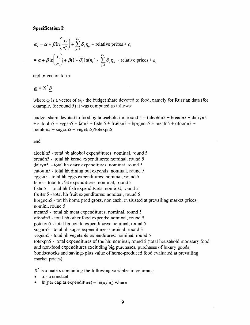
Specification I:

09i = a +±lniI + 95j)1j + relative prices 4

K-I

a + Ilnti) + 8( - 0) ln(n,) + E35j q7,, + relative prices +6,

and in vector-form:

o)= X'8

where o is a vector of (oi - the budget share devoted to food, namely for Russian data (forexample, for round 5) it was computed as follows:

budget share devoted to food by household i in round 5 = (alcohln5 + breadn5 + dairyn5+ eatoutn5 + eggsn5 + fatn5 + fishn5 + fruitsn5 + hprgncn5 + meatn5 + ofoodn5 +potaton5 + sugam5 + vegetn5)/totexpn5

and

alcohln5 - total hh alcohol expenditures: nominal, round 5breadn5 - total hh bread expenditures: nominal, round 5dairyn5 - total hh dairy expenditures: nominal, round 5eatoutn5 - total hh dining out expends: nominal, round Seggsn5 - total hh eggs expenditures: nominal, round 5fatn5 - total hh fat expenditures: nominal, round 5fishn5 - total hh fish expenditures: nominal, round 5fruitsn5 - total hh fruit expenditures: nominal, round 5hprgncn5 - tot hh home prod gross, non cash, evaluated at prevailing market prices:nominl, round 5meatn5 - total hh meat expenditures: nominal, round 5ofoodn5 - total hh other food expends: nominal, round 5potaton5 - total hh potato expenditures: nominal, round 5sugarn5 - total hh sugar expenditures: nominal, round 5vegetn5 - total hh vegetable expenditures: nominal, round 5totexpn5 - total expenditures of the hh: nominal, round 5 (total household monetary foodand non-food expenditures excluding big purchases, purchases of luxury goods,bonds/stocks and savings plus value of home-produced food evaluated at prevailingmarket prices)

X* is a matrix containing the following variables in columns:* oa - a constant* ln(per capita expenditure) = ln(x,/ nj) where

9

x; - total household expenditures (e.g. for round 5 totexpn5)n,- household size (e.g. for round 5 hhsize5)

* ln(n,)* n j- proportion of household members in a given demographic group j

K -=8 number of demographic groups. Namely, the following demographic groups wereused (e.g. for round 5):

fO_13_5 - women in age group 0-13f14_25_5 - women in age group 14-25f26_p5 - women in age group 26-55felder_5 - women in age group 55 and oldermO_13_5 men in age group 0-13ml14_25_5 - men in age group 14-25m26_p_5 - men in age group 26-60melder_5 - men in age group 60 and older

The demographic group ml 4_25_5 was excluded from regression to avoidmulticolliniarity and should be viewed as a reference group when analyzing coefficientson other demographic variables.

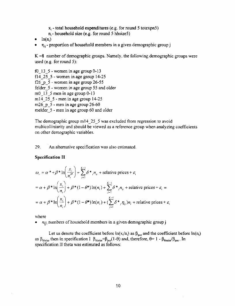
29. An alternative specification was also estimated.

Specification II

) K-1~~~K-(n°-)Z ,5 {n,, + relative prices+ El

= a +,B* In( +, * (I - -*) ln(ni) + E±5 *,n,, + relative prices + ,=

= a' + 8 * In( ni ) + j * (I1 - O*) In(n, ) + ( *, 7{j )nj + relative prices + c,

wherenij numbers of household members in a given demographic group j

Let us denote the coefficient before ln(x,/n1) as Ppce and the coefficient before ln(n,)as 3hh,size then in specification I f3hhsize4=pce0 -0) and, therefore, 0= 1 - PhNiAN/ Inspecification II theta was estimated as follows:

10

E 17ij E a r7y F. E X*e

9=0*iJ=: O* J1 = i='1;0=0S*- i=' n, * - n, = 1 ,8st n,

evaluating mjj and ni at their sample mean points.

30. If the estimated 0 appears to be equal to I then there is no economies of size inhousehold consumption and a per capita consumption poverty standard is appropriate(composition effects are controlled for in this regression). But in order to make inferencesabout theta we need to compute its variance which could be done through the delta-method as 0 is a non-linear function of estimated coefficients.

This method yields the following formula for estimating variance of theta:

[ar() £99 £9dO0 i var(/3,1,,.,) cov(I30,h,i: i,.p((. ) ,var(0) X ,,, iLcov(,8,,,,; ( /r, ) var(=/).() £90

where derivatives and variances are evaluated at estimates of r31111i1e and 3pce.

For specification I we haveS ~ ~I oS A,I,.i

- =_pand 2

and for specification Il:

£99 I £9l9 +8I:6 +(#i272)=-- and =

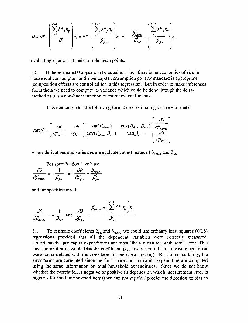
31. To estimate coefficients P.,, and , we could use ordinary least squares (OLS)regressions provided that all the dependent variables were correctly measured.Unfortunately, per capita expenditures are most likely measured with some error. Thismeasurement error would bias the coefficient p,, towards zero if this measurement errorwere not correlated with the error terms in the regression (£j ). But almost certainly, theerror terms are correlated since the food share and per capita expenditure are computedusing the same information on total household expenditures. Since we do not knowwhether the correlation is negative or positive (it depends on which measurement error isbigger - for food or non-food items) we can not a priori predict the direction of bias in

11

,0pc. Therefore, we need to find an instrumental variable (IV) in order to obtain unbiasedestimates of the coefficients. Household income is highly correlated with expendituresand since it is measured in a different way from expenditure (excluding income fromhome produced food which is an imputed term in both income and expenditures andwhich could introduce common errors) it is proposed that measurement errors in cashincome and expenditure are not correlated. Therefore, we could use cash per capitaincome as an instrumental variable for per capita expenditures.

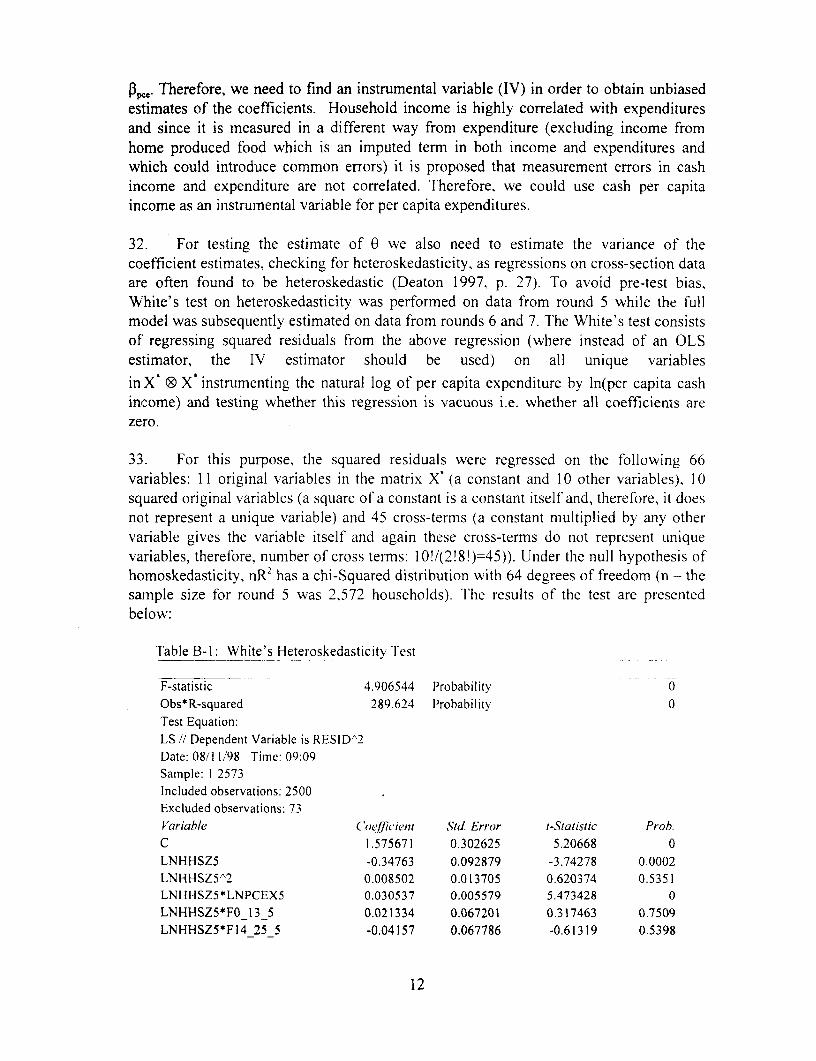
32. For testing the estimate of 0 we also need to estimate the variance of thecoefficient estimates, checking for heteroskedasticity, as regressions on cross-section dataare often found to be heteroskedastic (Deaton 1997, p. 27). To avoid pre-test bias,White's test on heteroskedasticity was performed on data from round 5 while the fullmodel was subsequently estimated on data from rounds 6 and 7. The White's test consistsof regressing squared residuals from the above regression (where instead of an OLSestimator, the IV estimator should be used) on all unique variables

in X 0 X instrumenting the natural log of per capita expenditure by ln(per capita cashincome) and testing whether this regression is vacuous i.e. whether all coefficients arezero.

33. For this purpose, the squared residuals were regressed on the following 66variables: 11 original variables in the matrix X* (a constant and 10 other variables), I0squared original variables (a square of a constant is a constant itself and, therefore, it doesnot represent a unique variable) and 45 cross-terms (a constant multiplied by any othervariable gives the variable itself and again these cross-terms do not represent uniquevariables, therefore, number of cross terms: I0!/(2!8!)=45)). Under the null hypothesis ofhomoskedasticity, nR' has a chi-Squared distribution with 64 degrees of freedom (n - thesample size for round 5 was 2,572 households). The results of the test are presentedbelow:

Table B-I: Wlhite's Heteroskedasticity lVcst

F-statistic 4.906544 Probability 0Obs*R-squared 289.624 Probability 0Test Equation:LS // Dependent Variable is RESID^2Date: 08/11/98 Time: 09:09Sample: 1 2573Included observations: 2500Excluded observations: 73Variable C'oefkicient Sid. Err(or f-Statistic Prob.C 1.575671 0.302625 5.20668 0LNHHSZ5 -0.34763 0.092879 -3.74278 0.0002LNHHSZ5^2 0.008502 0.013705 0.620374 0.5351LNHHSZ5*LNPCEX5 0.030537 0.005579 5.473428 0LNHHSZ5*FO_13_5 0.021334 0.067201 0.317463 0.7509LNHHSZ5*F14_25_5 -0.04157 0.067786 -0.61319 0.5398

12

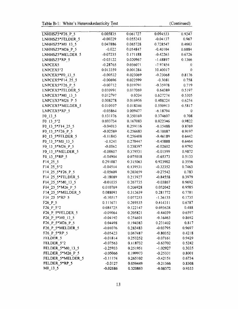
Table B-I: White's Heteroskedasticity Test (Continued)

LNHHSZ5*F26_P_5 0.005835 0.061727 0.094533 0.9247LNHHSZ5*FELDER_5 -0.00229 0.055243 -0.04137 0.967LNHHSZ5*M0_13_5 0.047886 0.065728 0.728547 0.4663LNHHSZ5*M26_P_5 -0.022 0.054847 -0.40104 0.6884LNHHSZ5*MELDER_5 -0.07235 0.171188 -0.42263 0.6726LNHHSZ5*RP_5 -0.03122 0.020967 -1.48897 0.1366LNPCEX5 -0.28765 0.036071 -7.97454 0LNPCEX5A2 0.013359 0.001284 10.40017 0LNPCEX5*FO_13_5 -0.00532 0.023069 -0.23068 0.8176LNPCEX5*F14_25_5 -0.00696 0.022599 -0.3081 0.758LNPCEX5*F26_P_5 -0.00712 0.019791 -0.35978 0.719LNPCEX5*FELDER_5 0.010991 0.017069 0.64389 0.5197LNPCEX5*MO_13_5 0.012797 0.0204 0.627274 0.5305LNPCEX5*M26_P_5 0.008278 0.016956 0.488224 0.6254

LNPCEX5*MELDER_5 0.010107 0,018346 0.550913 0.5817

LNPCEX5*RP_5 -0.05864 0,009477 -6.18794 0FO_13_5 0.131176 0.350169 0.374607 0.708

FO_13_5A2 0.003734 0.167083 0.022346 0.9822FO_13_5*F14_25_5 -0.04013 0.259116 -0.15488 0.8769FO_13_5*F26_P_5 -0.02589 0.256683 -0.10087 0.9197FO_13_5*FELDER_5 -0.11843 0.256408 -0.46189 0.6442FO_13_5*MO_13_5 -0.1241 0.270447 -0.45888 0.6464F0_13_5*M26_P_5 -0.0062 0.238397 -0.02602 0.9792F0_13_5*MELDER_5 -0.00607 0.379531 -0.01599 0.9872FO_13_5*RP_5 -0.04904 0.075018 -0.65373 0.5133F14_25_5 0.291087 0.315063 0.923902 0.3556F14_25_5^2 -0.04514 0.139531 -0.32352 0.7463

F14_25_5*F26_P_5 -0.05609 0.203659 -0.27542 0.783F14_25_5*FELDER_5 -0.18089 0.213927 -0.84558 0.3979F14_25_5*M0_13_5 -0.01035 0.267735 -0.03867 0.9692

F14_25_5*M26_P_5 0.010769 0.206928 0.052042 0.9585F14_25_5*MELDER_5 0.088093 0.312639 0.281772 0.7781F14_25_5*RP_5 -0.10517 0.077253 -1.36135 0.1735F26_P_5 0.111671 0.269535 0.414311 0.6787

F26_P_5`2 0.084725 0.122147 0.693628 0.488F26_P_5*FELDER_5 -0.09064 0.205821 -0.44039 0.6597

F26_P_5*MO_13_5 -0.04192 0.254601 -0.16463 0.8692F26_P_5*M26_P_5 0.04498 0.194383 0.231402 0.817

F26_P_5*MELDER_5 -0.01076 0.283483 -0.03795 0.9697F26_P_5*RP_5 -0.05423 0.067487 -0.80352 0.4218FELDER_5 -0.01814 0.253252 -0.07161 0.9429FELDER_5A2 -0.07563 0.118732 -0.63702 0.5242

FELDER_5*MO013_5 -0.25933 0.251951 -1.02927 0.3035FELDER_5*M26_P_5 -0.05066 0.199973 -0.25331 0.8001FELDER_5*MELDER_5 -0.11174 0.265102 -0.42151 0.6734FELDER_5*RP_5 -0.0127 0.059449 -0.21366 0.8308MO_13_5 -0.02686 0.320863 -0.08372 0.9333

1:3

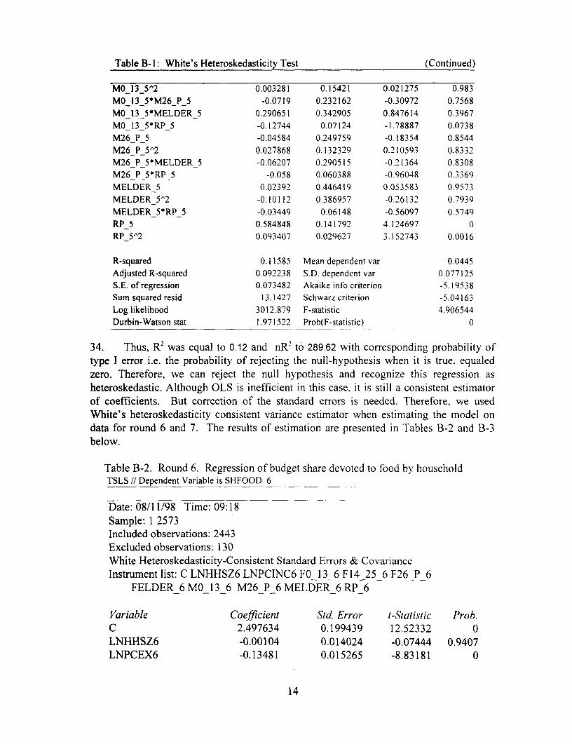
Table B-I: White's Heteroskedasticity Test (Continued)

MO 13_5A2 0.003281 0.15421 0.021275 0.983MO_13_5*M26_P_5 -0.0719 0.232162 -0.30972 0.7568MO_13_5*MELDER_5 0.290651 0.342905 0.847614 0.3967MO_13_5*RP_5 -0.12744 0.07124 -1.78887 0.0738M26_P_5 -0.04584 0.249759 -0.18354 0.8544M26_P_5A2 0.027868 0.132329 0.210593 0.8332M26_P_5*MELDER_5 -0.06207 0.290515 -0 t 364 0.8308M26_P_5*RP_5 -0.058 0.060388 -0.96048 0.3369MELDER_5 0.02392 0.446419 0.053583 0.9573MELDER_5A2 -0.10112 0.386957 -0.26132 0.7939MELDER_5*RP 5 -0.03449 0.06148 -0.56097 0.5749RP_5 0.584848 0.141792 4.124697 0RP_5^2 0.093407 0.029627 3.152743 0.0016

R-squared 0.11585 Mean dependent var 0.0445Adjusted R-squared 0.092238 S.D. dependent var 0.077125S.E. of regression 0.073482 Akaike info criterion -5.19538Sum squared resid 13.1427 Schwarz criterion -5.04163Log likelihood 3012.879 F-statistic 4.906544Durbin-Watson stat 1.971522 Prob(F-statistic) 0

34. Thus, R2 was equal to 0.12 and nR2 to 289.62 with corresponding probability oftype I error i.e. the probability of rejecting the null-hypothesis when it is true, equaledzero. Therefore, we can reject the null hypothesis and recognize this regression asheteroskedastic. Although OLS is inefficient in this case, it is still a consistent estimatorof coefficients. But correction of the standard errors is needed. Therefore, we usedWhite's heteroskedasticity consistent variance estimator when estimating the model ondata for round 6 and 7. The results of estimation are presented in Tables B-2 and B-3below.

Table B-2. Round 6. Regression of budget share devoted to food by houselholdTSLS 1/ Dependent Variable is SHFOOD 6

Date: 08/11/98 Time: 09:18

Sample: 1 2573Included observations: 2443Excluded observations: 130White Heteroskedasticity-Consistent Standard Errors & CovarianceInstrument list: C LNHHSZ6 LNPCINC6 FO 13 6 F14 25 6 F26_P_6

FELDER_6M0_13_6 M26_P_6MELDER 6RP6 _ _

Variable Coefficient Std. Error t-Statistic Prob.C 2.497634 0.199439 12.52332 0LNHHSZ6 -0.00104 0.014024 -0.07444 0.9407LNPCEX6 -0.13481 0.015265 -8.83181 0

14

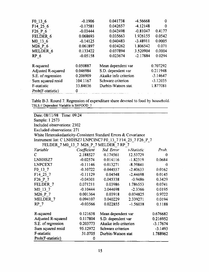
FO_13_6 -0.1906 0.041738 -4.56668 0F 14_25 6 -0.17581 0.042657 -4.12148 0F26_P_6 -0.03444 0.042498 -0.81047 0.4177FELDER_6 0.068693 0.035663 1.926155 0.0542MO_13_6 -0.14125 0.040483 -3.48911 0.0005M26_P_6 0.061897 0.034262 1.806542 0.071MELDER_6 0.133422 0.037894 3.520904 0.0004RP_6 -0.05158 0.023674 -2.17884 0.0294

R-squared 0.050887 Mean dependent var 0.707292Adjusted R-squared 0.046984 S.D. dependent var 0.211948S.E. of regression 0.206909 Akaike info criterion -3.14647Sum squared resid 104.1167 Schwarz criterion -3.12035F-statistic 33.84636 Durbin-Watson stat 1.877081Prob(F-statistic) 0

Table B-3. Round 7. Regression of expenditure share devoted to food by household.TSLS 11 Dependent Variable is SHFOOD_7

Date: 08/11/98 Time: 09:24Sample: 1 2573Included observations: 2302Excluded observations: 271White Heteroskedasticity-Consistent Standard Errors & CovarianceInstrument list: C LNHHSZ7 LNPCINC7 FO 13_7 F14_25_7 F26_P_7

FELDER_7 M0_13_7 M26_P_7 MELDER_7 RP_7Variable Coefficient Ski, Error -,Sitiistic Pioh.C 2.188527 0.174561 12.53729 0LNHHSZ7 -0.02574 0.014116 -1.82319 0.0684LNPCEX7 -0.11146 0.013271 -8.39841 0FO_13_7 -0.10722 0.044557 -2.40633 0.0162F14_25_7 -0.11129 0.04548 -2.44698 0.0145F26_P_7 -0.04301 0.045338 -0.9486 0.3429FELDER_7 0.071211 0.03986 1.786553 0.0741MO_13_7 -0.10444 0.044698 -2.3366 0.0195M26_P_7 0.001364 0.03918 0.034825 0.9722MELDER_7 0.094107 0.040229 2.339271 0.0194RP_7 -0.03566 0.022855 -1.56038 0.1188

R-squared 0.121638 Mean dependent var 0.676682Adjusted R-squared 0.117804 S.D. dependent var 0.216952S.E. of regression 0.203773 Akaike info criterion -3.17674Sum squared resid 95.12972 Schwarz criterion -3.1493F-statistic 31.0705 Durbin-Watson stat 1.788962Prob(F-statistic) 0

15

35. Analyzing these results we can estimate 0 as I - I,Iislze/p'pce= I - (-0.001 04)/( -0.13481)=0.99 for round 6 and 1-(-0.02574)/(-0.II146)=0.77 for round 7. To test whetherO is equal to 1 we have to compute the variance of theta (the tables presented thevariances Of Phhsize and Pc, only). The relevant parts of the variance-covariance matrix forthese two coefficients for rounds 6 and 7 are:

Table B-4: Variance-covariance matrix elements for testing hypothesis 0=1

Round 6C LNHHSZ6 LNPCEX6

C 0.039776 -0.00148 -0.00297LNHHSZ6 -0.00148 0.000197 9.70E-05LNPCEX6 -0.00297 9.70E-05 0.000233

Round 7C LNHHSZ7 LNPCEX7

C 0.030472 -0.0012 -0.00223LNHHSZ7 -0.0012 0.000199 6.95E-05ILNPCEX7 -0.00223 6.95E-05 0.000176

36. The corresponding estimates for the variance of theta calculated by the delta-tnethod are as follows: for round 6 var(0)=0.01 1 which yields the Wald test statistic of0.0089 for round 6 when testing the null hypothesis that 0=1 and for round 7 var(O)=0.014wvhich yields a Wald test statistic of 3.75. Under the null hypothesis of 0=1, the Wald teststatistics have a Chi-squared distribution with one degree of freedom (in case of a singlecoefficient the square root of the Wald test statistic is equivalent to the t-statistics whichare 0.094 and 1.93 in round 6 and 7 respectively). In both cases at 5% level ofsignificance we can not reject the null-hypothesis and can view 0 as indistinguishablefrom unity (Table B-5). This means that there are no significant economies of scale inconsumption.

37. As it was mentioned, another specification of the above regression (specificationIl) was estimated as well. For rounds 6 and 7, the corresponding estimates of 0 were 0.99and 0.92 (we have not computed the variance here).

38. Furthermore, similar regressions to the above were run with the share of the basicneeds bundle, namely, expenditures on food, shelter (rent and utilities) and clothes intotal household expenditures as the dependent variable. In this case, estimates for round 6and 7 were 0.97 and 0.74 and their variances were 0.013 and 0.022 respectively. Againthe Wald-test statistics which were 0.0651 and 3.07 (corresponding t-statistics are 0.26aind 1.75) show that at 5% significance level the hypothesis of 0 being equal to I can notbe rejected.

16

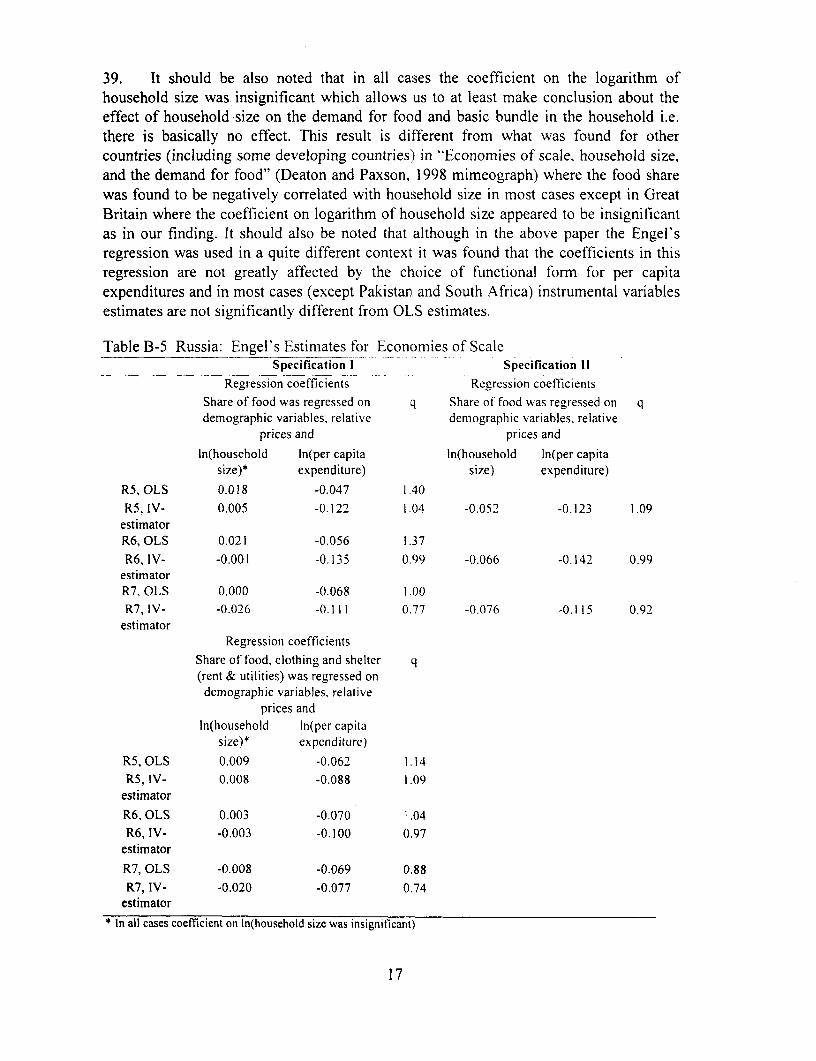
39. It should be also noted that in all cases the coefficient on the logarithm ofhousehold size was, insignificant which allows us to at least make conclusion about theeffect of household size on the demand for food and basic bundle in the household i.e.there is basically no effect. This result is different from what was found for othercountries (including some developing countries) in "Economies of scale, household size,and the demand for food" (Deaton and Paxson, 1998 mimeograph) where the food sharewas found to be negatively correlated with household size in most cases except in GreatBritain where the coefficient on logarithm of household size appeared to be insignificantas in our finding. It should also be noted that although in the above paper the Engel'sregression was used in a quite different context it was found that the coefficients in thisregression are not greatly affected by the choice of functional form for per capitaexpenditures and in most cases (except Pakistan and South Africa) instrumental variablesestimates are not significantly different from OLS estimates.

Table B-5 Russia: Engel's Estimates for Economies of ScaleSpecification I Specification 11

Regression coefficients Regression coefficients

Share of food was regressed on q Share of food was regressed on qdemographic variables, relative demographic variables, relative

prices and prices and

ln(household ln(per capita ln(household ln(per capitasize)* expenditure) size) expenditure)

R5, OLS 0.018 -0.047 1 40R5, IV- 0.005 -0.122 1.04 -0.052 -0.123 1.09estimatorR6, OLS 0.021 -0.056 1.37

R6, IV- -0.001 -0.135 0.99 -0.066 -0.142 0.99estimatorR7, OLS 0.000 -0.068 1.00R7, IV- -0.026 -0.111 0.77 -0.076 -0.115 0.92

estimatorRegression coefficients

Share of food, clothing and shelter q(rent & utilities) was regressed ondemographic variables, relative

prices andln(household ln(per capita

size)* expenditure)

R5, OLS 0.009 -0.062 1.14R5, IV- 0.008 -0.088 1.09

estimatorR6. OLS 0.003 -0.070 1.04R6, IV- -0.003 -0.100 0.97

estimatorR7, OLS -0.008 -0.069 0.88R7, IV- -0.020 -0.077 0.74estimator

*In all cases coefficient on ln(household sizc was insignificant)

17

POVERTY LINE USED IN THE STUDY

40. The measure of well-being which we used to identify the poor for Russian povertyy

assessment was as follows: resources per equivalent adultn,, + 09nh, +0.63n,,

where Y are total resources of the household, nad is the number of adults in the household,nCh is the number of children in the household, and nCId is the number of elderly in thehousehold and these resources were compared to the regional poverty line for adultsconstructed for eight regions of Russia as a population weighted average across 78official regional subsistence minimum for adults (Table B-6) (to match the sample)'. Itshould be noted though that depending on the choice of poverty line and parameter 0conclusions about poverty composition and rates may significantly vary.

41. It should be noted that the coefficients were used were constant, calculated fromthe official data for 1994. Goskomstat Rossii provided information on average povertylines for the 89 oblasts of Russia, but not the detailed information on how this average isbroken down into the child, adult, and elderly subcomponents for 1995 and 1996. Sincethese coefficients have changed very little over the time of the study, we simply appliedthe 1994 breakdown to 1995 and 1996. Strictly speaking, we should have requested theadditional information from Goskomstat Rossii and used slightly different breakdownsfor 1995 and 1996.

42. Relative prices were computed based on the regional poverty lines calculated bythe Ministry of Labor (prozhitochniy minimum). Eight regions were used for regressionanalysis:o Major metropolitan areas (Moscow and Moscow region, St. Petersburg and

Leningradsky region)* North and Northwestern regions* Central and Central black-earth regions

Volga and Volgo-Vyatsky regions* North Caucasus* Ural* West Siberian region* East Siberian region and Far East.

43. Relative prices and regional poverty lines calculations are presented in AnnexThree, pages 15-17.

44. Table B-7 below presents average household size of the poor and non-poor aswell as poverty rates for different values of 0 (a sensitivity analysis for 0). Lanjouw,Paternosto and Milanovic (1998) suggested that a critical value for 0 would be 0.7*

2 Division into regions

18

check, at which there would be reversals of policy advice to target children over theelderly. At such a 0, the poverty rate would be 25.* percent. It is important tounderstand that policy reversals are not only driven by estimates of 0 but also by wherethe poverty line is drawn. For example, at a very high poverty line (many of thepopulation would be poor), the share of elderly in the poor might be much higher, whileat a very low poverty line (very few of the population would be poor), the share ofchildren in the poor could be very high. This finding demonstrates the process of whichoverall changes in headcount fluctuate with applying higher at lower poverty lines (TableB-8). The table demonstrates that there is definitely some bunching of people around theimmediate poverty line, since a proportional change in the poverty line is exceeded by theresulting change in the headcounts. For example. reducing the poverty line by 10 percentresults in a 15 percent reduction in the resulting headcount. Although some bunching isclearly noticeable, the extent here seems to be in the distribution of consumption less thanobserved for the early rounds of the RLMS (World Bank, 1995).

19

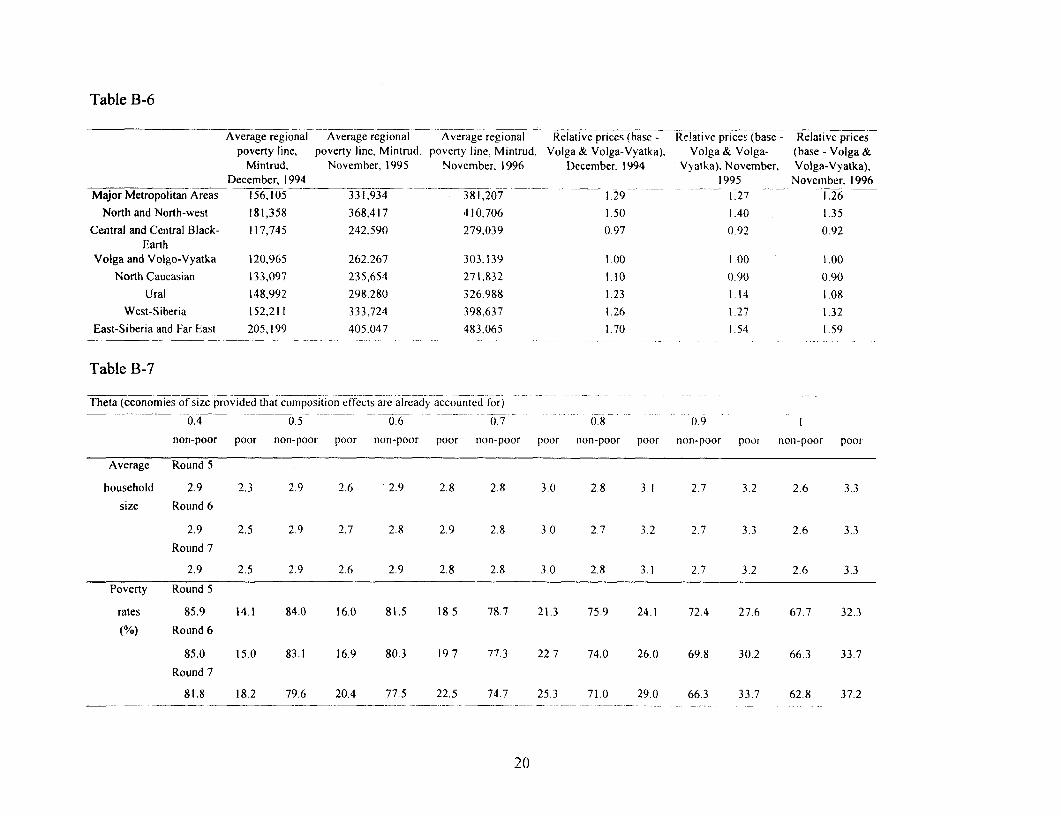
Table B-6

Average regional Average regional Average regional Relative prices (base - Relative prices (base - Relative pricespoverty line, poverty line, Mintrud. poverty line, Mintrud, Volga & Volga-Vyatka), Volga & Volga- (base - Volga &

Mintrud, November, 1995 November, 1996 December. 1994 Vyatka). November, Volga-Vyatka),December, 1994 ____ ___l995_ _----1995 November, 1996

MajorMetropolitan Areas 156,105 331,934 381,207 1.29 1.27 1.26

North and North-west 181,358 368.417 410.706 1.50 1.40 1.35

Central and Central Black- 117,745 242.590 279.039 0.97 0.92 0.92Earth

Volga and Volgo-Vyatka 120,965 262,267 303.139 1.00 1.00 1.00

North Caucasian 133,097 235.654 271.832 1.10 0.9( 0.90

Ural 148,992 298.280 326.988 1.23 1.14 1.08

West-Siberia 152,211 333,724 398,637 1.26 1.27 1.32

East-Siberia and Far East 205,199 405.047 483.065 1.70 1.54 1.59

Table B-7

Theta (economies of size provided that composition effects arc already accounted for)

0.4 0.5 0.6 0.7 (.8 (.9

non-poor poor non-poor poor non-poor poor non-poor poor non-poor poor non-poor poor non-poor poor

Average Round 5

household 2.9 2.3 2.9 2.6 2.9 2.8 2.8 3.0 2.8 3.1 2.7 3.2 2.6 3.3

size Round 6

2.9 2.5 2.9 2.7 2.8 2.9 2.8 3.0 2.7 3.2 2.7 3.3 2.6 3.3

Round 7

2.9 2.5 2.9 2.6 2.9 2.8 2.8 3.0 2.8 3.1 2.7 3.2 2.6 3.3

Poverty Round 5

rates 85.9 14.1 84.0 16.0 81.5 18.5 78.7 21.3 75.9 24.1 72.4 27.6 67.7 32.3

(%) Round 6

85.0 15.0 83.1 16.9 80.3 19.7 77.3 22 7 74.0 26.0 69.8 30.2 66.3 33.7

Round 7

81.8 18.2 79.6 20.4 77.5 22.5 74.7 25.3 71.0 29.0 66.3 33.7 62.8 37.2

20

Table B-8. Russia: Poverty Sensitivity, 1994-96

World Poverty Poverty Poverty Poverty 10% Decrease 20% Decrease 10% Increase 20% Increase

Bank Line= Line= Line= Line= & Change & Change & Change & Change

Estimate 1/ 90% 80% 110% 120% in Headcount in Headcount in Headcount in Headcount

(In percent of population/individuals 2/)

1994 37.6 32.0 26.6 42.4 46.3 14.9 29.3 -12.8 -23.1

1995 39.6 34.2 29.9 44.7 50.3 13.6 24.5 -12.9 -27.0

1996 43.1 38.3 31.8 48.0 52.1 11.1 26.2 -11.4 -20.9

(In percent of households)

1994 32.2 27.1 22.4 36.6 40.2 15.8 30.4 -13.7 -24.8

1995 33.7 28.7 24.6 38.2 43.2 14.8 27.0 -13.4 -28.2

1996 37.1 32.8 27.3 41.6 45.3 11.6 26.4 -12.1 -22.1

Source: Author calculations from RLMS.

Notes: First column is baseline estimates for the Russian Povert) Assessment Update.

Columns labeled Poverty Line = show the headcounts that would result if a poverty line x percent lower or higher were used.

TIhe remaining columns show the percent change in headcounts (retferencing the baseline estimates in the flirst column) that resulted fromapplying a lower or higher poverty line

I/ Russian L.ongitudinal Monitoring Survey (panel households only) All-Russia Subsistence Minimum. Author calculations

2/ Grossed up to individuals by veighting by household size in each round.

21

*~~~~~~~~~~~~~~~~

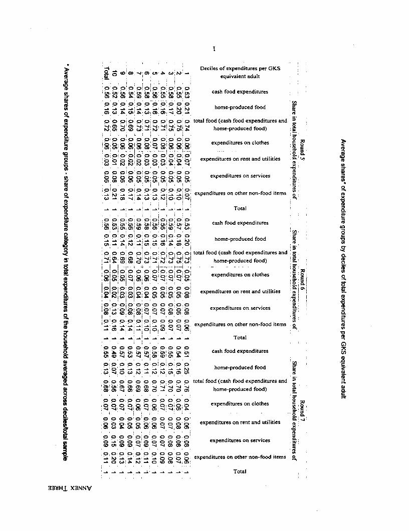
;I _ 1 Deciles of expenditures per GKSta U ! i . equivalent adultDii

O O '0 0 0 0 o 0 0 0) rx 6,i A 6 cash food expenditures

=r cn N3 0) J co Ctt, 0r OD1 3. CJIDi~~~~~~~~~~~~~~~~~~~~~~~~~~:

On _j _ _ _' _ _ _ _ i N Nhome-produced foodo0S w5 v 4n W! cn.cn o-

*D o o 0 o o o0 0 o 0o total food (cash food expenditures and 5'O ;_-40 -J0) -4 -4 :-4 -41 --J-4-.

oD N' Vl O Wj ui ! home-produced food)Q ~~~~~~~~~." ; . 1 , ) ," Ml home

-' ~ ~~~~~~ O aO C 0 0 0 0 ;1 oi OJ a 0-. 0o 0 0 0lo 0 0 0 0 0 expenditures on clothes 0'1> 00en 0 010000 0 c 0 0 c c

* . , ., . . ,. ............... 'CO...4.......... j , ) .- .

O,O;O'O O O O 0'0I0000 0 0 -. ID00000000000 o o o o o ooo expenditures on rent and utilities - '-ai

C )0 !~ 0 CD 0 0 C)a

* o'o olo o o o o o o a) Do o 010 0: 0 0 0 oo 0 expenditures on services ,

0D 0). 00 VlI c.n cn cn - 01

0 0'o ooIoooC)oo '° t ' N-a-a-a -a--a ' X . * ' oC exp enditures on other non-food items C

eD~~~~~~~~~~0 W 4 - C_, W W .N) 9 C ° ° -I4 -x ' '

-a-a _ t , _; v 1 *, ^ ' _ sTotal

- .0 0,0W010 0'pp:ao a0iO0 CD 0 _-- 00i 0 t9 .' I ! il- 0 cash food expenditures

00 0w 01 0o OD 0 0j 0O 0 0

g o .°lQ!°;Q C°P.° o ohome-produced foodcn .8h, arl I tn (M -bl OD 3

3~~~~~. 1. .| ':1J ') '~ ' 0_ic

- o oCoo o oio ol .Cj totalf tashfood oodexpendituresand o0ic) -M 4 ~-41 -4, -4 -4 -4J-. 41 aj

3 cno o C!>¢ N cn t' 0 home-produced food) 0- o- OiOl0trO oltI- --ot-I i - - -Di o 00 o}0I0000] o o! o! ol o iexpenditures on clothes - 0IS~~~~~~~!a 01a 0,000 :c 23<C X x- D+C 1 -4 i-i 4 1 -4 i i4 L,iii

j~~ooooooo~~~0 ooC) (DI~ 0 |ojoo 0ki 000 jt 0 expendituresonrentandutilities ol !i

0. x.~~~~~~~~~~~~~~~~~~~a,Ci)v Ni C;[ X ~ i ^1 C:) C:) C:): C:) ! t 0c I I . . i X

0, a' 0! O C> 0 00000 00 expenditures on services 0.o~~~~~~~D j to CO CO! !-,-4 4 0C.0,C

=D P,P _. p _ _ _ _; _ o; o O expenditures on other non-food items_ cn D .... O 0,_ o C.D 4 ) on oh i o 0

01

i Q . D D C, . . ao 6J .01 eJ in b 6 6sc1 bn '.? <n cash food expenditures ;jo L" C D: -t W. 4 _1 C CO L'0 ! -J J

'C 0 0C0)0 0 C 01 0' 0 0 00oD ~. . .. home-produced foodm - - - - - - - ¢ j

o oo o o o 0 o o o o 0 total food (cash food expenditures and 30)0)CJ) 0)QS.I')IM-4 -4 'I -4 -4 a)-

Di co 0 c.4 CO CO CD O C- 0 0) home-produced food) Din ~. . . . . . . . . . . .

n ,o~~~~~~~~~~ . .o.o .i . . .0 expenditures on clothes C_;0s ~ ~ ~ ~~~~~~~~~ t : CD i -: - l : -i- -. -

0~~~~~~~~~~~~~~~~~~~~

0000000000O O O 0 expenditu res nt and utilities F c°nw COP can 0:0 _t 9 C- Co c)) xo o.o o o o o o o o o =~~~~~~~~~~~~~~~~~~~~~~~~~~~o~

o - 0 00 0 0 o o o o expenditures on services 00 Un W (D -4 W -4 40OD0

o , 0 0 O 3 CD Eo~~~~ 0 0 0 0 0 0 0 0 exediue on sevie

_ - - C) _ C)ooo 0 expenditures on other non-food items0 - .6 M 0 (0D co -4 ca)

- -a - -a-a - - - Total

33QH1 X3NNV

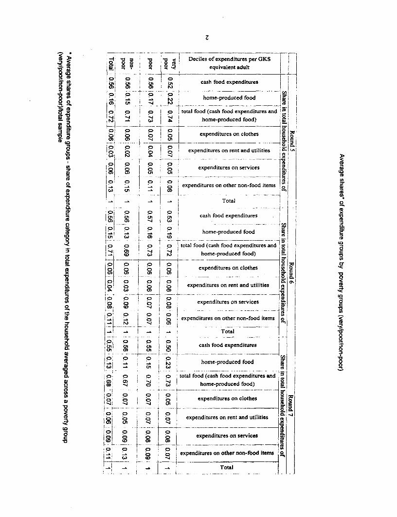
> la a 1 r ^ - o 1 < Deciles of expenditures per GKS

5- ; 1 1equivalent adultfi _ __ _ .J____ _.4. _. f

0 L" ° o°l ! cn C e0 0 cash food expenditures0), 0) ! ) I_I, I

cO 8 ' ° ° ° T t°0 home-produced food K/'1L- ~- .s IN -

x C, a o o i oi total food (cash food expenditures and ItD -4 :-4 -0

- I mJ 9 t X E k 2 home-produced food) __

v i ° l ° ° I ° [ expenditures onclothesi> N a~~~~~) -4 1--s!'t1 - >a

r to ° ' O | o } expenditures on rent and utilities Ci L

0 ~~~~I r-i b. _4 >

0~~~~00 o o o I oI i

0 CD I)

:r ~~ ! 0 ) ] expenditres.on services t

CD - I cn - _ _ _ ___- ca

° -I o ~ 0 ] x , expenditures on other non-food items 01CD C.) Cln _ I I 1

.:1, _ ! 4 Total

Cn C o * ° cash food expenditures xa lol o I o ! o ] 4lW- :CD (D CL------- - J

0s 0 0_ I _ i , _ i home-produced food co ,) 0,) <, _,_ _ , ----- - - 5

.o o o o total food (cash food expenditures and oc-4 0) -4~ :- I 0

to ^4! a) _ _ 9 ; home-produced food) v

0D o - a°o oo O | expenditures on clothes o3< ~~ 0 ' 5

tab C> CD a 0 1 0 expenditures on rent and utilities aA0 >1 t3~~w ) co Xg Q

0 . o o fo oD expenditures on services a c0~~~~~~0 C

=0 0D 0 0 CA ICD expenditures on other non-food items o D

o . ~~~~~~_ ._ . ___.

c . -, ' Total

=r C j> _ 0hm-rdcdfo 0 C" CA h f O , O tot food (cash food expenditures

home-produced food

aw CD, CD O o total food (cash food expenditures and

0 00,~ -4 0: C. home-produced food)0o l,._ 0 ._ 0 0 .

31 JO ° ° ° io expenditures on clothes

-ji o4 -4 L- o oi

CD ~~~~~~~~expenditures on rent and utilities '

i(DD 0 10 ~~~~expenditures on services

iojexpenditures on other non-food items 1

I I J Total

x -s 0 < ! r = I t - - < I Deciles of expenditures per GKS

000 0 Or I2m 3 0 equivalent adult |

_~~~~~ Foo o o -ttCD~~~~~~~* ~ :us .o i o 3 co en z O | cash food expenditures

c o I O ~~a O CD O Ct) ~< 0 0~~~~ - - _ ----- --- -_ _ _ _ _ _ _

= fD (-at 0 0 home-produced food _ 0

M K) ~~~~~~~~~~home-produced food)I! a 0 0 ototal food (cash food expenditures and i

i3 a f a>! a) F ) home-produced food) i

-10 i 0 0 o 1 0 1 expenditures on clothesX ~ ~ 0 0 0111X 4._

3 r | O > o f T0o expenditures on rent and utilities Q I C

3~~~~' w -n IX

° ~ ~~~~~ - ---- t---t--- --- - -

eD 1 ° ° ° I o ° iexpenditures on services j 3I4 -4 (C) 0) 0

0 0 I 0 v | o ! expenditures on other non-food items o01 C) CD_

oi _ I | !Total j!- ~~~~~~~~0

01 01 cash food expenditures CD-~~ 01 - --- -------------.------ ~ ~V CD

home-produced food .

0 0 0 ,o o total food (cash food expenditures and osr.o __ _ 9 home-produced food) I <

*0~~~~~~~~~~~~~~~~~~n X o o O ~~~~~~~~~~ex.pe-nd-i-tur-e-s on c-lothes <

o 0 4 .0'c

expenditures on rent and utilities c oe L~~~~CA)_ w cn _ x _ _ _,

0

o.. -1 ° 0 ° J °expenditures on services .-

0 1- - .O - -0- 0 -

a _j I C) p expenditures on other non-food items o.b . n ._ _ , _ _ .

Total :

t en; .v + cn t crl ~~~cash food expenditures !I

5KX 1Or O , t 1 shome-produced foodf- 0i1 C0 - t-

2 0 0 | O | o k o , total food (cash food expenditures and | IL"l CM 9 ) :-4 aw j home-produced food)

01 0 0 O p O , expenditures on clothes i W3 ~ 0 0) Co expenditures on

o co O CsC

m .--- _--- __ . - - ---- - - -

C 40 0 0) 0.I-..3 6 ~~~~~~~~~~~~~~~~~~expenditures on rent and utilities eV

_ _: _ o O 8 O expenditures on services

expenditures on other non-food items O |

_ i L1 Total... i . J J _L ,_ __ ._ ___

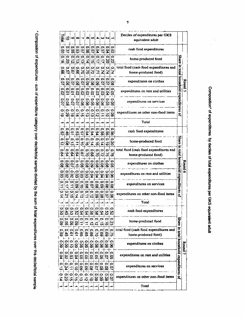
* V r i - - - - - r -- r- - - - . ----

*or-r . --r- L -I ~ I~ I ....- ! |Deciles of expenditures per GKSo g 0 .J co C?' 1 O en v CDequivalent adult3_ P0Po 'Po - ° 0 ,, cash food expenditures

0-401cm C." C." ur O ~ ~~~~~~~ 000 0- -½ ----(D > o .° l ° l ° ° l *° l *° jo tJ i home-produced food

-X -0 P&IP 0 0 0A homx 0) 6 Po I ' --4- IM _-'4 ---

ta o o 14I o o o~ | o o o o o ototal food (cash food expenditures and

CL 0 ) --C -4 -J - o . -A. .01 home-produced food)

CD_ -. t- -o .o -o o o o o o

C) o C) a ° 00 Co C C oo CD expenditures on clothes- ) - O -4 - -D - -4 -4 CD,R -o sts o~~~p' oI o I o ovCC 000 000 000

oo o o 0 o oo expenditures on rent and utilities M. 0<0 _. _*_ . __ . _ . _ .____. ___ x .

x o ooO expenditures on servicesn~~~~~- 00 -4 -4 4mL cn aa Ul n" 4c, IoCD -

. . - - -- ------ +- -- -- - - - - -- - ---- _ , I-o jo 0 o _ o -o o | ° l ° l ° oexpenditures on other non-food items

sa I~~~~CD eoCD CD tnw cJ wlm CDo CO o

-X . v; .~ -- - z v a v } _ Total

0 e n 00^9 1 C0 0 cash food expenditures

o 0) N" T>- T W | 1|v O' CS - -) (A.. CD~~~~~~~~~~~~C

a ~ ~~~ 1 l°l°.. 11°l° l .° home-produced food

(> CDo p p o oC 0 op o a a total food (cash food expenditures and |

l -4 CD1 OD 0 CA1N| C"| ahome-produced food) 2. 0

A) pppOoCooCOCP CDC)O:p @-'.OOOOOO. . expenditures on clothes C; |

3 t t~~~D - C) C)>X e 40 0o cxlCDI -- ____4oli ea~~~~~0 lol alo OD OD CDOD O ODo QV1o

Ca 0 C)P 9 0C0)0 0 0 0 0 expenditures on rent and utilities

5D PPPOOO0 OOO. LA 0 ° l a expenditures on services c|

w- I~~~-I4ji°°cl11°aco IRI co co c.9 I0 00000 000 I

(D [-; N t-L-t-&-0 _~ 6 o l o | o | * |expcnditures on other non-food itemsc k -| k- |- +. |.' |--&- 0 0 -- 0.. . ... CD~~~~-l u -h j C o-

3 - \ |- 1 i -1 1 1-} .- '. Total

- 01~~~~( C) a C 01 i 301 01 arCA tn tn } t ° ol ocash food expenditures

x C, °°°°i°°°_ _ home-produced food|x (s0 ! 0g 0 91 I 0 h r food

a I o | o rco CD o0 0 total food (cash food expenditures and C0)~~~O) - 0) ho-

CD Lo | -1 j ° ! 0 i o co tn home-produced food)|I

0 P010 ~~~~~D IPCD lolo ololo olojo,C)o o expenditures on clothes

(ID cUIo w C<DcoCD to o 0D CI<:O <i n CD~~~~~~~~~~~~~~~~~~~~~~~.C

@ o 0 of o 000000 expenditures on rent and utilitiesCD :'. CD I > |0' - | 0 (0 | 0D 0 0 es n s

tD °)NO|-°|°|°J°J°1*C) °°6°|°a expenditures on services |

Q)! Cj C) CD _ expenditures on other non-food items OjA) .b 0 1 01'01'C,)l N) olco Co o cj

CD ,-!-1-1-1-1- !-'j-'-l-' Total

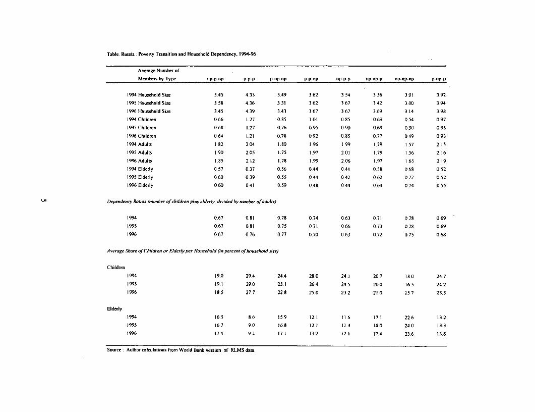
Table. Russia Poverty Transition and Household Dependency. 1994-96

Average Number of

Members by Type np-p-np p-p-p p-np-np p-p-np np-p-p np-np-p np-np-np p-np-p

1994 Household Size 3.45 4.33 3.49 3.62 3 54 3 36 3.01 3.92

1995 Household Size 3 58 4.36 3.31 3.62 3 67 3 42 3.00 3.94

1996 Household Size 3.45 4.39 3 43 3.67 3 67 3 69 3.14 3.98

1994 Children 0 66 1.27 0.85 1 01 0 85 0 69 0.54 0.97

1995 Children 0 68 1 27 0.76 0 95 0 90 0 69 0 50 0.95

1996 Children 0 64 1 21 0.78 0.92 0.85 0 77 0 49 0 93

1994 Adults 1 82 204 1 80 1.96 1.99 1.79 1.57 2 15

1995 Adults I 90 2.05 1.75 1 97 2.01 1.79 1.56 2.16

1996 Adults 1 85 2 12 1 78 1.99 2.06 1.97 1 65 2.19

1994 Elderly 0 57 0 37 0 56 0 44 0.41 0.58 0.68 0.52

1995 Elderly 0 60 0 39 0 55 0.44 0.42 0.62 0 72 0 52

1996 Elderly 0 60 0.41 0 59 0.48 0 44 0 64 0 74 0 55

U' Dependency Ratios (number of children plus elderly, divided by number of adlults)

1994 0 67 0 81 078 0.74 0 63 0 71 0.78 0.69

1995 0 67 0.81 0.75 0.71 0 66 0.73 0 78 0.69

1996 0.67 0.76 0 77 0.70 0.63 0.72 0 75 0 68

Average Share of Children or Elderly per Household (in percent of household size)

Children

1994 19.0 29.4 24.4 280 24 1 207 180 24.7

1995 19.1 29.0 23.1 26.4 24.5 200 16 5 24.2

1996 18.5 27.7 22.8 25.0 232 21.0 157 23.3

Elderly

1994 16.5 8.6 15.9 12.1 11 6 17 1 22.6 13 2

1995 16.7 9.0 16. 12 1 11 4 IS0 240 13.3

1996 17.4 92 17.1 132 12 1 174 23.6 13.8

Source: Author calculations from World Bank version of RLMS data.

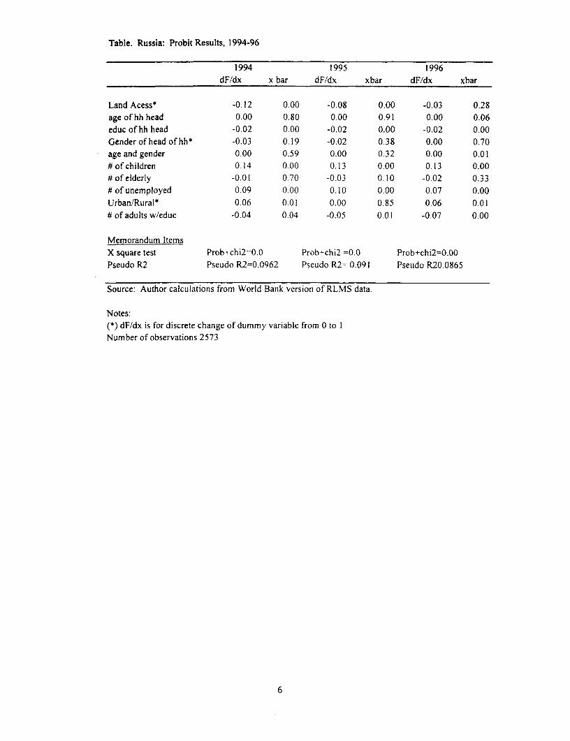
Table. Russia: Probit Results, 1994-96

1994 1995 1996dF/dx x bar dF/dx xbar dF/dx xbar

Land Acess* -0.12 0.00 -0.08 0.00 -0.03 0.28age of hh head 0.00 0.80 0.00 0.91 0.00 0.06educ of hh head -0.02 0.00 -0.02 0.00 -0.02 0.00Genderofheadofhh* -0.03 0.19 -0.02 0.38 0.00 0.70age and gender 0.00 0.59 0.00 0.32 0.00 0.01#ofchildren 0.14 0.00 0.13 0.00 0.13 0.00# of elderly -0.01 0.70 -0.03 0.10 -0.02 0.33# of unemployed 0.09 0.00 0.10 0.00 0.07 0.00Urban/Rural* 0.06 0.01 0.00 0.85 0.06 0.01# of adults w/educ -0.04 0.04 -0.05 0.01 -0.07 0.00

Memorandum ItemsX square test Prob+chi2=0.0 Prob+chi2 =0.0 Prob+chi2=0.00Pseudo R2 Pseudo R2=0.0962 Pseudo R2= 0.091 Pseudo R20.0865

Source: Author calculations from World Bank version of RLMS data.

Notes:(*) dF/dx is for discrete change of dummy variable from 0 to INumber of observations 2573

6

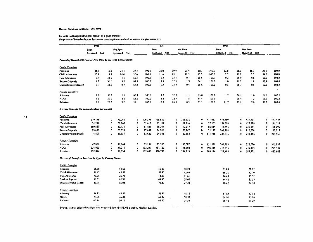
RuJs;: Incidence Analysis. 1994-1996

Ex-Ante Consumption (without receipt of a given transfer)(In percent of households poor by ex-ante consumption calculated as without the given tranfer)

1994 1995 1996Poor Not Poor Poor Not Poor Poor Not PoorReceived Not Received Not Received Not Received Not Received Not Received Not

Percentef anseholds Poer er Non-Poor by Ex-A ate Consumnptioe

I'ublhc TransferPensions 28.9 17.5 24.1 29.5 100.0 26.0 19.6 25.4 29.1 100.0 23.6 26.3 16.3 33.9 100.0Child Allowance 13.1 199 14 4 52 6 1000 11 6 23 1 103 55.0 100.0 7.7 30.6 7.3 54.5 100.0Fuel Allowance 0.9 31 6 1 1 66.5 100.0 0.3 33.5 07 65.6 1000 0.2 36.9 0.g 62.0 100.0Student Stipends 1 7 306 3.2 64.5 100.0 1 4 32.5 1.9 64 1 100.0 I 0 36.2 I 8 60.9 100.0UnenploymentlBenefit 07 316 07 670 100.0 0.7 33.0 0.4 65 g 100.0 05 367 0.5 62.2 100.0

Plr,wje TrunsfrsAlimony 16 30 8 1 1 664 1000 1 3 32.7 1.1 65 0 1000 1.2 36 1 1.0 61.7 100 0NGOs I 5 309 2.1 65.6 100.0 1.4 32.7 1.5 644 100.0 I 1 364 12 61.3 100.0Relatives 96 252 9.2 56.1 1000 10.0 26.4 8.3 55.3 100.0 11.7 29.1 9.0 50.3 100.0

A verage Transfer (in nomiunl rwbies per month)

Public Tranm.ersPensions 179,136 0 173,060 0 176.374 318.622 0 303,238 0 311,017 478,189 0 439,693 0 462,431Child Allowance 34.218 0 29,260 0 31,617 85,107 0 69,116 0 77,565 154,599 0 127,589 0 141,514Fuel Allowance 100,680 0 30,121 0 61,801 56,303 0 102,217 0 88.25 155,855 0 120,165 0 128,096Student Stipends 29,676 0 26,558 0 27,638 74,246 0 75,847 0 75.177 162,718 0 112,23S 0 132,017Unemployment Benefit 74,809 0 89,957 0 82,600 128,566 0 82,664 0 111,736 223,236 0 235,883 0 229,560

Private fransfersAlimony 67,051 0 81,%9 0 73,144 122,506 0 143,007 0 131,581 365,985 0 222,000 0 302,833NGOs 234,065 0 59.211 0 132,227 431,729 0 175,202 0 298,335 316,645 0 236,313 0 274,437Relatives 192,824 0 129,934 0 162,095 370,793 0 234,753 0 309,114 529,495 0 283,872 0 422,642

Percent of Transfers Receivesd by Type by Poverty Status

l'ublic TransfersPensions 55.38 44 62 51.S0 48.20 61 08 38.92Child Allowance 51.47 4853 57.97 42.03 5621 4379Fucl Allowance 73.25 26.75 1.39 81 61 26.68 73 32Student Stipends 37.03 6297 4140 58.60 44.45 5555Unemployment Benefit 43.95 56.05 72.80 2720 48.62 51.38

1'rivale 7ruan.ferAlimony 54.13 45.87 51.85 48 15 67.82 32 18NGOs 73.96 26.04 69.42 30.58 54 90 45 10Relatives 60.84 3916 65.50 34 50 70.78 2922

Source. Author calculations from data extracted from the RLMS panel by Michael Lokshin.

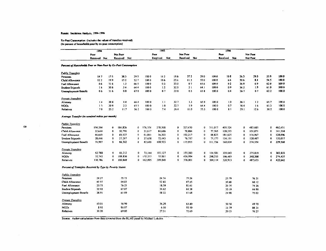
Russia: Incidence Analysis, 1994-1996

Ex-Pos4 Consumption (includes the values of transfers rceived)(In percent of households poor by ex-post consumption)

1994 1995 1996Poor Not Poor Poor Not Poor Poor Not PoorReceived Not Received Not Received Not Received Not Received Not Not Poor

Perewt ef Haesehb Poor or I N0 -?.. by Ex-Post C.auamption

Public TransfersPensions 14.7 17.5 38.3 29.5 100.0 14 2 19.6 37.2 29.0 100.0 10.R 26.3 29.0 33.9 100.0Child Allowance 12.2 19.9 152 52.7 100.0 10.6 23.1 11.3 55.0 100.0 6.6 306 8.4 54.5 100.0Fuel Allowance 06 31 6 1.3 66.5 1000 03 33.5 0.7 65.6 100.0 0.2 36.9 09 62.0 100.0StudentStipends 1.6 306 34 644 100.0 1.2 32.5 21 64.1 1000 0.9 36.2 1.9 610 100.0Unemployment Benefit 0 6 31.6 0.8 67 0 100 0 0.7 33.0 0.5 65.8 100.0 0.4 36.7 0.7 62.2 100.0

Private 7ranfersAlimony 14 308 14 664 2000 1.1 32.7 1.3 65.0 1000 10 36.1 1.2 61.7 100.0NGOs 13 309 2.3 655 1000 1.0 32.7 1.9 64.4 00.0 07 36.4 1.6 61.3 100.0Relatives 70 25.2 11.7 56.2 1000 7.4 264 11.0 55.3 000 8 1 29.1 1226 50.2 100.0

A verage Trasfer (in nominal rubles per month)

Puhlic TranIfersPensions 154,294 0 184,S26 0 176,374 278,508 0 323,430 0 311,017 405.524 0 483.685 0 462,431Child Allowance 32,644 0 30,791 0 31,617 84.686 0 70,884 0 77,565 128,215 0 151.871 0 141,514Fuel Allowance 46,669 0 69,137 0 61,801 56,303 0 102,217 0 88,825 181,025 0 116,067 0 128,096Student Stipends 28,446 0 27.267 0 27.638 72,443 0 76.717 0 75,177 134,151 0 128,407 0 132,017Unemployment Benefit 74,997 0 88,302 0 82.600 108,923 0 115,955 0 111.736 160.024 0 274.554 0 229,560

P1rinae IrunsfersAlimony 62,788 0 83.212 0 73,144 103,527 0 155,383 0 131,581 335,043 0 275,819 0 302,833NGOs 32,742 0 188.830 0 132,227 55,861 0 426,994 0 298,335 106,403 0 348,208 0 274,437Relatives 130,786 0 180.860 0 162,095 209,840 0 376,001 0 309,114 320,913 0 487,635 0 422.642

Percent of Transfers Received by Type by Poverty Status

I'ublic TransfersPensions 24.27 75.73 24.74 75 26 23 79 76 21Child Allowance 45 97 54.03 52.85 47.15 39.88 60 12Fuel Allowance 23.75 76.25 18.39 81.61 25 74 74 26Student Stipends 32 93 67.07 34.62 65.38 33.10 66 90Unemployment Benefit 38.91 61.09 58.32 4L.68 24.98 7502

Private TratsuersAlimony 43.01 56.99 36,20 63.80 50.30 49 70NGOs 8.93 91.07 6 50 93.50 11.79 S8 21Relatives 30.20 69.80 27 31 72 69 29.73 70 27

Source: Author calculations from data extracted from the RLMS panel by Michael Lokshin

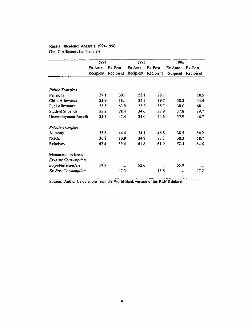
Russia: Incidence Analysis, 1994-1996

Gini Coefficients for Transfers

1994 1995 1996Ex Ante Ex-Post Ex Ante Ex-Post Ex Ante Ex-PostRecipient Recipient Recipient Recipient Recipient Recipient

Public TransfersPensions 59.1 30.1 52.1 29.1 28.5Child Allowance 35.9 38.1 34.5 39.7 38.3 44.4Fuel Allowance 35.5 63.9 33.9 55.7 38.0 68.1Student Stipends 35.2 28.4 34.0 37.9 37.8 39.7Unemployment Benefit 35.4 47.4 34.0 44.6 37.9 46.7

Private TransfersAlimony 35.6 44.4 34.1 46.8 38.5 54.2NGOs 36.8 80.9 34.9 77.3 38.3 58.7Relatives 42.4 59.4 41.8 61.9 52.5 64.4

Memorandum ItemsEx-Ante Consumption,no public transfers 59.9 ... 52.6 ... 55.9 ...Ex-Post Consumplion ... 47.3 ... 43.8 ... 47.2

Source: Author Calculations from the World Bank version of the RLMS dataset.

9

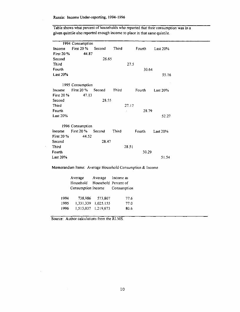
Russia: Income Under-reporting, 1994-1996

Table shows what percent of households who reported that their consumption was in agiven quintile also reported enough income to place in that same quintile.

1994 ConsumptionIncome First 20 % Second Third Fourth Last 20%First 20 % 44.87Second 26.65Third 27.5Fourth 30.64Last 20% 55.16

1995 ConsumptionIncome First 20 % Second Third Fourth Last 20%First 20 % 47.13Second 28.55Third 27.17Fourth 28.79Last 20% 52.27

1996 ConsumptionIncome First 20 % Second Third Fourth Last 20%First 20 % 44.52Second 28.47Third 28.51Fourth 30.29Last 20% 51.54

Memorandum Items: Average Household Consumption & Income

Average Average Income asHousehold Household Percent ofConsumption Income Consumption

1994 738,986 573,807 77.61995 1,331,339 1,025,155 77.01996 1,513,037 1,219,673 80.6

Source: Author calculations from the RLMS.

10

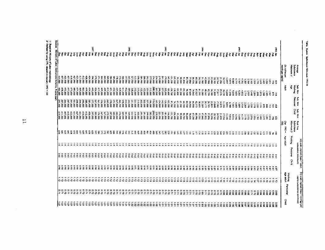
e., X a 3 i " 3~~~~. A

w > e; _ w w o o q S ° S ^ ^ eR J S S vo~~~~~~~~~ t *> t = ZJ ~-. 8 o^=- O - - - - -

- - - - - - - - - - - - W- o°ooeseWbW_eawbWSwbWwo_qw<wW

b~~~~~~~~~~~ ~ .bo bg go . .b .bg .b bo . .O bo bg . .g .g. °og °ooo oOOgOg=

I~~~~~~~~~~~~~~~~~~~~~~~~~~~~ ;0 .. 0 ...

a . . .o . . . . . . o o o o o o . . . . . . . . . . .

8 S S S S S S S S S S S S S S S S S S 8 S S S S S SS S @ 8 S S S 5 S S S S SS S S S S S S 4 Wo Wc Wo 8° S 9 ,oW oW oW CZ eW Wc C tW t0, qW Wa 0 qW, qW CO

______-- - - - - -- - - -- -_-__-_-_-- _-_- __-_-_-__-_-_--_-_-__-_-_--_-_-_--_-_-__-_-_-- - -

_------ __ __- __ __ __- -- _-- ------ _----_-_-----_---- o---3----°°°°_°°°_S°°°°°°22 22 ae 22 O -°°°°° O)O a 22a -°-°°M° 2°ERM°°-° -° °°°° °80 0°°2 °0a R°o°°°°°°'Dox°°¢°°> 'D 0 00

Table Russia: Ago-Gender Composition of Refugees and Forced Migrants(people)

Age Bracket Total % Males % Females %1,147,100 100% 534,103 47.3% 612,997 52.7%

0 to 5 96,631 100% 48,720 50.4% 47,911 49.6%6 to 15 232,975 100% 116,923 50.1% 116,052 49.9%Elderly* 648,048 100% 311,058 47.9% 336,990 52. 1%Able bodied Ages 169,446 100% 57,402 33.8% 112,004 66.2%Source: Official statisticsfromfamily budget survey: SotsialPnoye polozheniye i uroveni zhizni naseleniya

Rossiya 1997, p 33.

* men 16-59, women 16-54

12

Table Russia: Family Size and type(in thousands)

1970 1979 1989

Total number of Families 32,617 36,725 40,246Including:2 people 8,655 11,608 13,7593 people 9,116 11,589 11,2814 people 8,118 8,588 10,1545 people 6,728 4,940 5,052Average Size 4 3 3Nuclear Family 20,639 24,350 26,930Extended Family 5,128 4,692 4,614Complex Family 1,024 1,278 1,355Single Parent w/ children only 4,070 4,659 5,293Single Parent wl children+relatives 1,129 752 816Other 627 994 1,238Single person families 8,580 9,581 10,126Source: (Sotsial'noye polozheniye i uroveni zhizni naseleniya Rossiya 1997, p. 34.)

13

Russia: Pensioners by Type. 1990-1996(in Thousands End Year)

1990 1991 1992 1993 1994 1995 1996

All 32,848 34,044 35,273 36,100 36,623 37,083 37,827Old Age 25,659 27,131 28,390 29,021 29.095 29,011 29,081Disability 3,514 3,385 3,363 3,562 3,910 4,270 4,542Loss of Breadwinner 2,792 2,574 2,473 2,420 2,423 2,482 2,464Early Retirement 82 84 97 107 135 197 544Social I/ 470 870 956 990 1,060 1,123 1,196Source: Soisial'noye polozheniye i uroveni zhizni naseleniya Rossiya 1997, p. 197.

I/ Social Pensioners were fornerly called minimum pensioners. Social pensions are awarded to those who lack sufficientwork tenure for an old age pension.

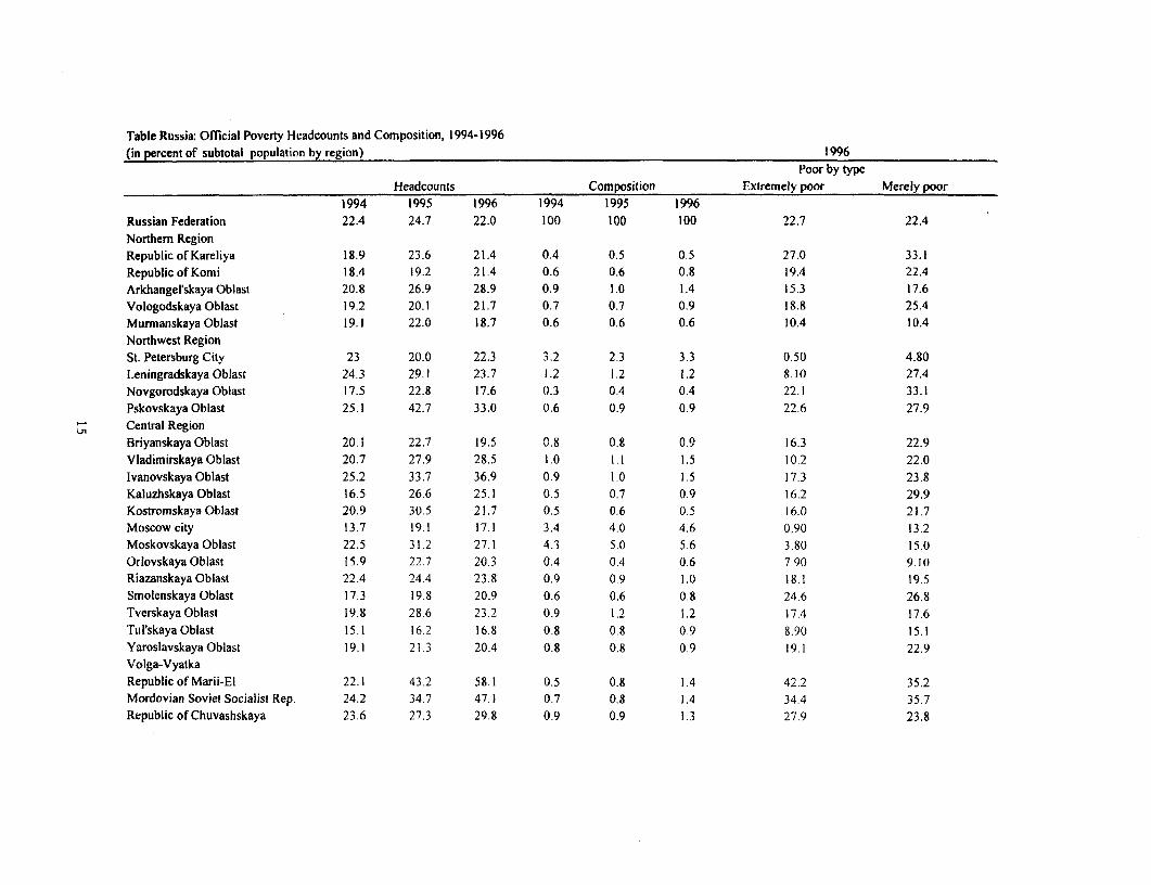
Table Russia: Official Poverty Headcounts and Composition, 1994-1996(in percent of subtotal population by region) 996

Poor by typeHeadcounts Composition Extremely poor Merely poor

1994 1995 1996 1994 1995 1996Russian Federation 22.4 24.7 22.0 100 100 100 22.7 22.4Northem RegionRepublic of Kareliya 18.9 23.6 21.4 0.4 0.5 0.5 27.0 33.1RepublicofKomi 18.4 19.2 21.4 0.6 0.6 0.8 19.4 22.4Arkhangel'skaya Oblast 20.8 26.9 28.9 0.9 1.0 1.4 15.3 17.6Vologodskaya Oblast 19.2 20.1 21.7 0.7 0.7 0.9 18.8 25.4MunnanskayaOblast 19.1 22.0 18.7 0.6 0.6 0.6 10.4 10.4Northwest RegionSt. Petersburg City 23 20.0 22.3 3.2 2.3 3.3 0.50 4.80Leningradskaya Oblast 24.3 29.1 23.7 1.2 1.2 1.2 8. 10 27.4NovgorodskayaOblast 17.5 22.8 17.6 0.3 0.4 0.4 22.1 33.1Pskovskaya Oblast 25.1 42.7 33.0 0.6 0.9 0.9 22.6 27.9Central RegionBriyanskayaOblast 20.1 22.7 19.5 0.8 0.8 0.9 16.3 22.9Vladimirskaya Oblast 20.7 27.9 28.5 1.0 1.1 1.5 10.2 22.0IvanovskayaOblast 25.2 33.7 36.9 0.9 1.0 1.5 17.3 23.8Kaluzhskaya Oblast 16.5 26.6 25.1 0.5 0.7 0.9 16.2 29.9Kostromskaya Oblast 20.9 30.5 21.7 0.5 0.6 0.5 16.0 21.7Moscow city 13.7 19.1 17.1 3.4 4.0 4.6 0.90 13.2Moskovskaya Oblast 22.5 31.2 27.1 4.3 5.0 5.6 3.80 15.0Orlovskaya Oblast 15.9 22.7 20.3 0.4 0.4 0.6 7.90 9.10Ria7anskayaOblast 22.4 24.4 23.8 0,9 0.9 1.0 18.1 19.5Smolenskaya Oblast 17.3 19.8 20.9 0.6 0.6 0.8 24.6 26.8TverskayaOblast 19.8 28.6 23.2 0.9 1.2 1.2 17.4 17.6Tul'skayaOblast 15.1 16.2 16.8 0.8 0.8 0.9 8.90 15.1Yaroslavskaya Oblast 19.1 21.3 20.4 0.8 0.8 0.9 19.1 22.9Volga-VyatkaRepublic ofMarii-EI 22.1 43.2 58.1 0.5 0.8 1.4 42.2 35.2Mordovian Soviet Socialist Rep. 24.2 34.7 47.1 0.7 0.8 1.4 34.4 35.7Republic of Chuvashskaya 23.6 27.3 29.8 0.9 0.9 1.3 27.9 23.8

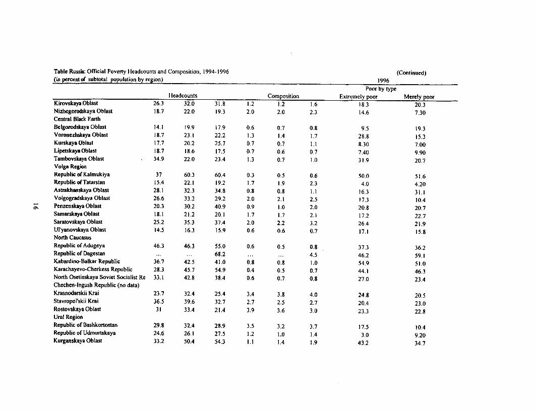
Table Russia: Official Poverty Ilcadcounts and Composition, 1994-1996 (Continued)(in percent of subtotal population by region) 1996

Poor by typeI leadcounts Composition Extremely poor Merely poor

Kirovskaya Oblast 26.3 32.0 31.8 1.2 1.2 1.6 18.3 20.3NizhegorodskayaOblast 18.7 22.0 19.3 2.0 2.0 2.3 14.6 7.30Central Black EarthBclgorodskayaOblast 14.1 19.9 17.9 0.6 0.7 0.8 9.5 19.3Voronezhskaya Oblast 18.7 23.1 22.2 1.3 1.4 1.7 28.8 15.3KurskayaOblast 17.7 20.2 25.7 0.7 0.7 1.1 8.30 7.00Lipetskaya Oblast 18.7 18.6 17.5 0.7 0.6 0.7 7.40 9.90Tambovskaya Oblast 34.9 22.0 23.4 1.3 0.7 1.0 31.9 20.7Volga RegionRepublic of Kalmukiya 37 60.3 60.4 0.3 0.5 0.6 50.0 51.6RepublicofTatarstan 15.4 22.1 19.2 1.7 1.9 2.3 4.0 4.20AstrakhanskayaOblast 28.1 32.3 34.8 0.8 0.8 1.1 16.3 31.1Volgogradskaya Oblast 26.6 33.2 29.2 2.0 2.1 2.5 17.3 10.4Penzenskaya Oblast 20.3 30.2 40.9 0.9 1.0 2.0 20.8 20.7SamarskayaOblast 18.1 21.2 20.1 1.7 1.7 2.1 17.2 22.7SaratovskayaOblast 25.2 35.3 37.4 2.0 2.2 3.2 26.4 21.9Ul'yanovskayaOblast 14.5 16.3 15.9 0.6 0.6 0.7 17.1 15.8North CaucasusRepublic of Adugeya 46.3 46.3 55.0 0.6 0.5 0.8 37.3 36.2Republic of Dagestan ... ... 68.2 ... ... 4.5 46.2 59.1Kabardino-Balkar Republic 36.7 42.5 41.0 0.8 0.8 1.0 54.9 51.0Karachayevo-Cherkess Republic 28.3 45.7 54.9 0.4 0.5 0.7 44.1 46.3North Osetinskaya Soviet Socialist Re 33.1 42.8 38.4 0.6 0.7 0.8 27.0 23.4Chechen-Ingush Republic (no data)Krasnodarskii Krai 23.7 32.4 25.4 3.4 3.8 4.0 24.8 20.5Stavropol'skii Krai 36.5 39.6 32.7 2.7 2.5 2.7 20.4 23.0RostovskayaOblast 31 33.4 21.4 3.9 3.6 3.0 23.3 22.8Ural RegionRepublic of Bashkortostan 29.8 32.4 28.9 3.5 3.2 3.7 17.5 10.4Republic of Udmurtskaya 24.6 26.1 27.5 1.2 1.0 1.4 3.0 9.20Kurganskaya Oblast 33.2 50.4 54.3 1.1 1.4 1.9 43.2 34.7

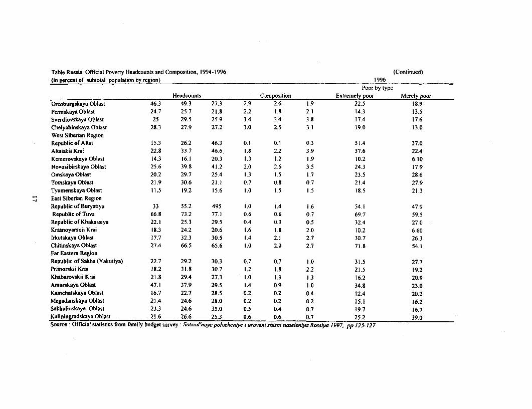
Table Russia: Official Poverty Headcounts and Composition, 1994-1996 (Continued)(in percent of subtotal population by region) 1996

Poor by typeHeadcounts Composition Extremely poor Merely poor

Orenburgskaya Oblast 46.3 49.3 27.3 2.9 2.6 1.9 22.5 18.9PermskayaOblast 24.7 25.7 21.8 2.2 1.8 2.1 14.3 13.5Sverdlovskaya Oblast 25 29.5 25.9 3.4 3.4 3.8 17.4 17.6Chelyabinskaya Oblast 28.3 27.9 27.2 3.0 2.5 3.1 19.0 13.0West Siberian RegionRepublicofAltai 15.3 26.2 46.3 0.1 0.1 0.3 51.4 37.0Altaiskii Krai 22.8 33.7 46.6 1.8 2.2 3.9 37.6 22.4Kemerovskaya Oblast 14.3 16.1 20.3 1.3 1.2 1.9 10.2 6.10Novosibirskaya Oblast 25.6 39.8 41.2 2.0 2.6 3.5 24.3 17.9Omskaya Oblast 20.2 29.7 25.4 1.3 1.5 1.7 23.5 28.6Tomskaya Oblast 21.9 30.6 21.1 0.7 0.8 0.7 21.4 27.9TyumenskayaOblast 11.5 19.2 15.6 1.0 1.5 1.5 18.5 21.3East Siberian RegionRepublic of Buryatiya 33 55.2 495 1.0 1.4 1.6 54.1 47.9Republic of Tuva 66.8 73.2 77.1 0.6 0.6 0.7 69.7 59.5Republic of Khakassiya 22.1 25.3 29.5 0.4 0.3 0.5 32.4 27.0Krasnoyarskii Krai 18.3 24.2 20.6 1.6 1.8 2.0 10.2 6.60IrkutskayaOblast 17.7 32.3 30.5 1.4 2.1 2.7 30.7 26.3Chitinskaya Oblast 27.4 66.5 65.6 1.0 2.0 2.7 71.8 54.1Far Eastern RegionRepublic of Sakha (Yakutiya) 22.7 29.2 30.3 0.7 0.7 1.0 31.5 27.7Primorskii Krai 18.2 31.8 30.7 1.2 1.8 2.2 21.5 19.2Khabarovskii Krai 21.8 29.4 27.3 1.0 1.3 1.3 16.2 20.9Amurskaya Oblast 47.1 37.9 29.5 1.4 0.9 1.0 34.8 23.0Kamchatskaya Oblast 16.7 22.7 28.5 0.2 0.2 0.4 12.4 20.2Magadanskaya Oblast 21.4 24.6 28.0 0.2 0.2 0.2 15.1 16.2Sakhalinskaya Oblast 23.3 24.6 35.0 0.5 0.4 0.7 19.7 16.7Kaliningradskaya Oblast 21.6 26.6 25.3 0.6 0.6 0.7 25.2 39.0Source: Official statistics from family budget survey: Sotsial'noyepolozheniye i urovenizhizni naseleniya Rossiya 1997. pp 125-127

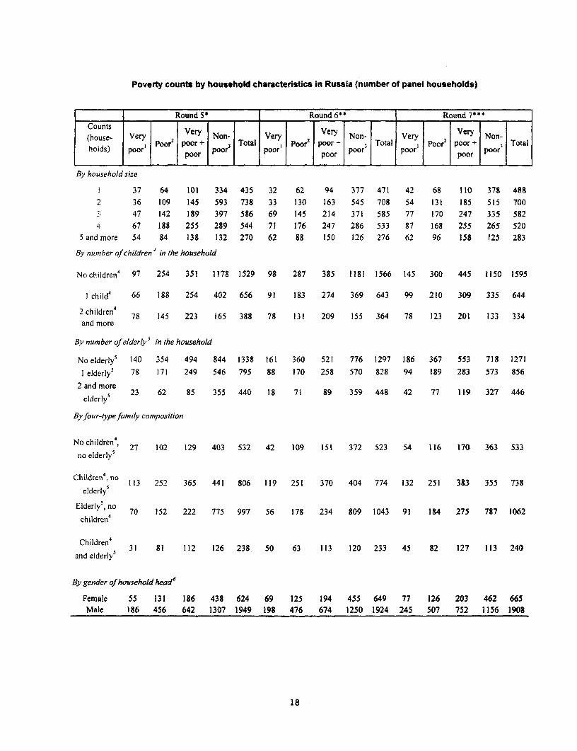
Poverty counts by household characteristics in Russia (number of panel households)

Round 5* Round 6** Round 7***

Cousnts Vr r Very Non- Very 2 Very Non- Very V2 ery Non-

holds) poor' poor + Total oor Poor poor - Total Poor poor poorTotalpoor poor poor

By household size

1 37 64 101 334 435 32 62 94 377 471 42 68 110 378 488

2 36 109 145 593 738 33 130 163 545 708 54 131 185 515 7003 47 142 189 397 586 69 145 214 371 585 77 170 247 335 5824 67 188 255 289 544 71 176 247 286 533 87 168 255 265 520

5 and more 54 84 138 132 270 62 88 150 126 276 62 96 158 125 283

By number of children in the household

Nochildren 4 97 254 351 1178 1529 98 287 385 1181 1566 145 300 445 1150 1595

I child4 66 188 254 402 656 91 183 274 369 643 99 210 309 335 644

2 children 4

78 145 223 165 388 78 131 209 155 364 78 123 201 133 334and more

By number of elderly' in the household

Noelderly' 140 354 494 844 1338 161 360 521 776 1297 186 367 553 718 1271

I elderly5 78 171 249 546 795 88 170 258 570 828 94 189 283 573 856

2 and moreeldmorl' 23 62 85 355 440 18 71 89 359 448 42 77 119 327 446elderly

Byfour-typefamily composition

No children4, 27 102 129 403 532 42 109 151 372 523 54 116 170 363 533no elderlys

4

Ciildren ,no 113 252 365 441 806 119 251 370 404 774 132 251 383 355 738elderly5

Elderly , no 70 152 222 775 997 56 178 234 809 1043 91 184 275 787 1062children

Childrenl3 31 81 112 126 238. 50 63 113 120 233 45 82 127 113 240and elderlyS

By gender of household head 6

Female 55 131 186 438 624 69 125 194 455 649 77 126 203 462 665Male 186 456 642 1307 1949 198 476 674 1250 1924 245 507 752 1156 1908

18

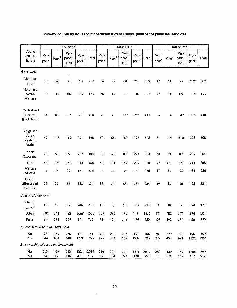
Poverty counts by household characteristics in Russia (number of panel households)

Round 5* Round 6** Round 7***Counts

(house- Very Very Non- Very 2 Very Non- Very Very Non-holds) poor' Poor2 poor + 3 Total l Poor poor + 3 Total pPoor 2 poor t Total

holds) poor poor poor poor poor poor poor poor

By regions

Metropo-letrop7 17 54 71 231 302 16 53 69 233 302 12 43 55 247 302lian7

North andNorth- 19 45 64 109 173 26 45 71 102 173 27 38 65 108 173

Western

Central andCentral 31 87 118 300 418 31 91 122 296 418 36 106 142 276 418

Black Earth

Volga and

Volgoa 52 115 167 341 508 57 126 183 325 508 71 139 210 298 508V.yatsky

basin

North 28 69 97 207 304 17 63 80 224 304 28 59 87 217 304Caucasian

Ural 45 105 150 238 388 40 111 151 237 388 52 121 173 215 388

Western 24 55 79 177 256 47 57 104 152 256 57 65 122 134 256Siberia

EasternSiberia and 25 57 82 142 224 33 55 88 136 224 39 62 101 123 224

Far East

By type of settlement

Metro-polies8 15 52 67 206 273 15 50 65 208 273 10 39 49 224 273

Urban 140 342 482 1068 1550 159 380 539 1011 1550 174 402 576 974 1550

Rural 86 193 279 471 750 93 171 264 486 750 138 192 330 420 750

By access to land in the household

No 97 183 280 471 751 92 201 293 471 764 94 179 273 496 769Yes 144 404 548 1274 1822 175 400 575 1234 1809 228 454 682 1122 1804

By ownership of car in the household

No 213 499 712 1324 2036 240 501 741 1276 2017 280 509 789 1206 1995Yes 28 88 116 421 537 27 100 127 429 556 42 124 166 412 578

19

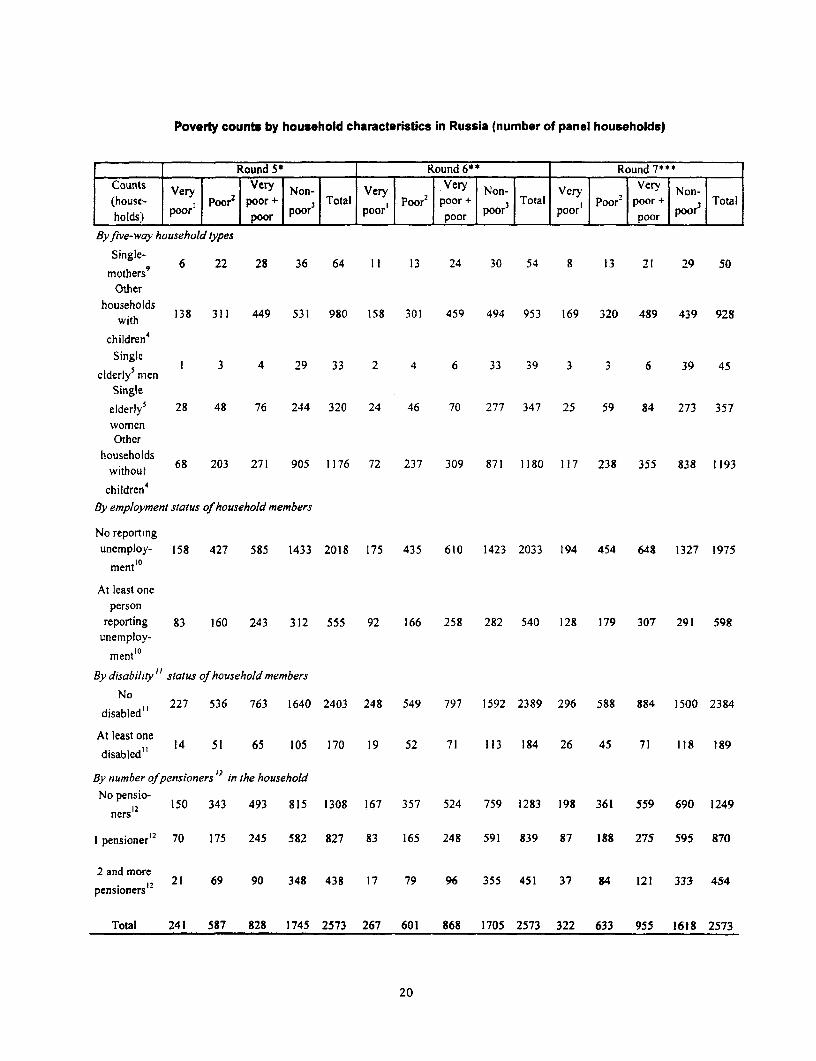
Poverty counts by household characteristics in Russia (number of panel households)

Round 5S Round 6* _ Round 7**lCounts Very Very Non- Very Very Non- Very Very Non-(house- P Poor2 poor + 3 Total poor2 poor + 3 Total l Poor poor + Totalholds) poor poor poor poor poor poor poor poor

Byfrve-way household types

Single- 6 22 28 36 64 11 13 24 30 54 8 13 21 29 50mothersg

Other

houshos 138 311 449 531 980 158 301 459 494 953 169 320 489 439 928

children4

Singl5e 1 3 4 29 33 2 4 6 33 39 3 3 6 39 45

elderly' menSingle

elderly5 28 48 76 244 320 24 46 70 277 347 25 59 84 273 357womenOther

householdswithout 68 203 271 905 1176 72 237 309 871 1180 117 238 355 838 1193

children4

By employment status of household members

No reportingunemploy- 158 427 585 1433 2018 175 435 610 1423 2033 194 454 648 1327 1975

ment'0

At least oneperson

reporting 83 160 243 312 555 92 166 258 282 540 128 179 307 291 598unemploy-

mentl'

By disability" status of household members

Nodisabled" 227 536 763 1640 2403 248 549 797 1592 2389 296 588 884 1500 2384

At least onedisabled" 14 51 65 105 170 19 52 71 113 184 26 45 71 118 189

By number of pensioners " in the householdNo pensio-

12 150 343 493 815 1308 167 357 524 759 1283 198 361 559 690 1249ners

I pensioner'2 70 175 245 582 827 83 165 248 591 839 87 188 275 595 870

2 and morepensioners'2 21 69 90 348 438 17 79 96 355 451 37 84 121 333 454

Total 241 587 828 1745 2573 267 601 868 1705 2573 322 633 955 1618 2573

20

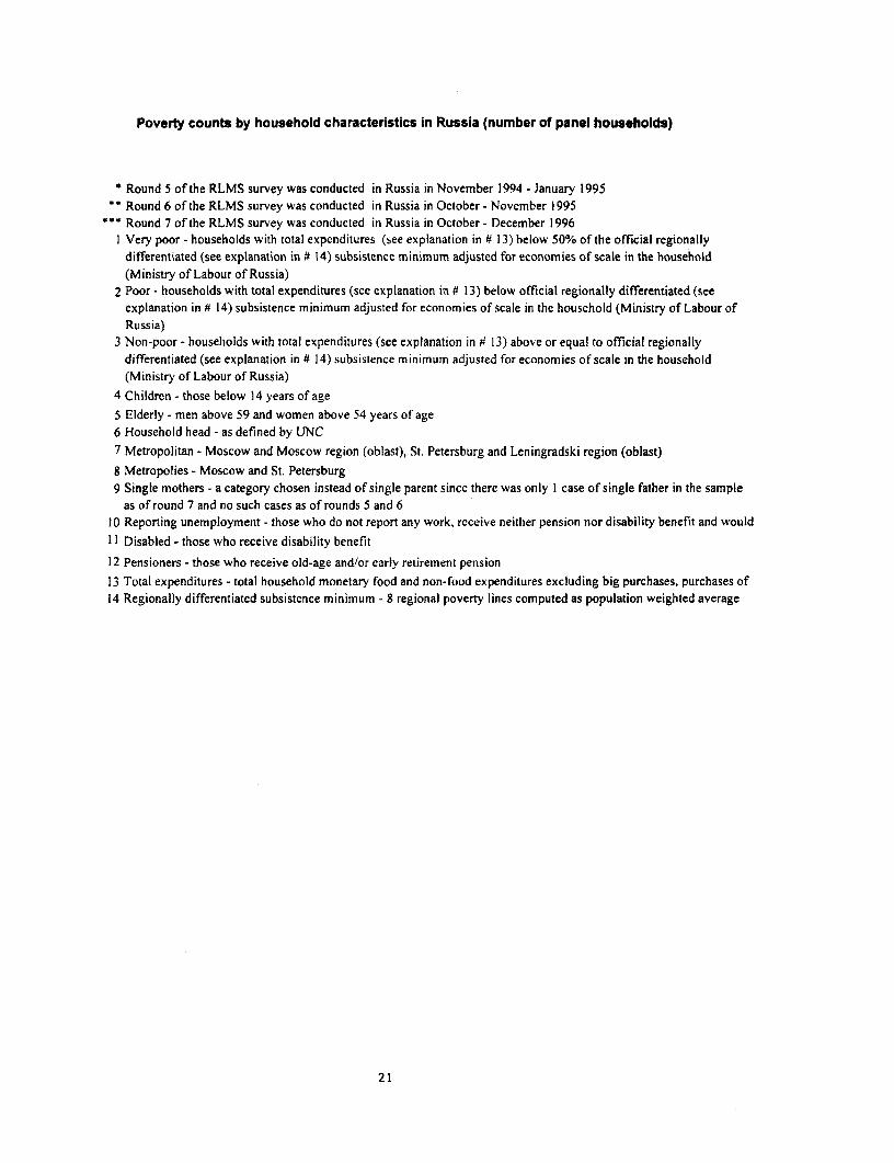
Poverty counts by household characteristics in Russia (number of panel households)

* Round 5 of the RLMS survey was conducted in Russia in November 1994 - January 1995** Round 6 of the RLMS survey was conducted in Russia in October - November 1995

$** Round 7 of the RLMS survey was conducted in Russia in October- December 19961 Very poor - households with total expcnditures (see explanation in # 13) below 50% of the official regionally

differentiated (see explanation in 4 14) subsistence minimum adjusted for economies of scale in the household(Ministry of Labour of Russia)

2 Poor - households with total expenditures (see explanation in # 13) below official regionally differentiated (seeexplanation in # 14) subsistence minimum adjusted for economies of scale in thc houschold (Ministry of Labour ofRussia)

3 Non-poor - households with total expenditures (see explanation in # 13) above or equal to official regionallydifferentiated (see explanation in # 14) subsistence minimum adjusted for economies of scale in the household(Ministry of Labour of Russia)

4 Children - those below 14 years of age5 Elderly - men above 59 and women above 54 years of age6 Household head - as defined by UNC7 Metropolitan - Moscow and Moscow region (oblast), St. Petersburg and Leningradski region (oblast)8 Metropolies - Moscow and St. Petersburg9 Single mothers - a category chosen instead of single parent since there was only I case of single father in the sample

as of round 7 and no such cases as of rounds 5 and 610 Reporting unemployment - those who do not report any work, receive neither pension nor disability benefit and wouldII Disabled - those who receive disability benefit

12 Pensioners - those who receive old-age and/or early retirement pension13 Total expenditures - total household monetary food and non-food expenditures excluding big purchases, purchases of14 Regionally differentiated subsistence minimum - 8 regional poverty lines computed as population weighted average

21

Poverty rates by household characteristics in Russia (% of panel households)

Round 5* Round 6** Round 7***Rates (0/6ooff Verv Vhouseholds) VerYPor Very Non- Very 2 Non- Very Vr-y Non-

poor or poor + po 3 Total oa1 Poor 2poor -i po 3 Total po'Poor'2 poor + por Totalpoor poor poor poopoor poor poor poor-

By household size

1 8.5 14.7 23.2 76.8 100.0 6.8 13.2 20.0 80.0 100.0 8.6 13.9 22.5 77.5 100.0

2 4.9 14.8 19.6 80.4 100.0 4.7 18.4 23.0 77.0 100.0 7.7 18.7 26.4 73.6 100.0

3 8.0 24.2 32.3 67.7 100.0 11.8 24.8 36.6 63.4 100.0 13.2 29.2 42.4 57.6 100.04 12.3 34.6 46.9 53.1 100.0 13.3 33.0 46.3 53.7 100.0 16.7 32.3 49.0 51.0 100.0

5and more 20.0 31.1 51.1 48.9 100.0 22.5 31.9 54.3 45.7 100.0 21.9 33.9 55.8 44.2 100.0

By number of children 4 in the household

Nochildren4 6.3 16.6 23.0 77.0 100.0 6.3 18.3 24.6 75.4 100.0 9.1 18.8 27.9 72.1 100.0

I child4 10.1 28.7 38.7 61.3 100.0 14.2 28.5 42.6 57.4 100.0 15.4 32.6 48.0 52.0 100.0

2children 4 and 20.1 37.4 57.5 42.5 100.0 21.4 36.0 57.4 42.6 100.0 23.4 36.8 60.2 39.8 100.0more

By number of elderly5 in the household

No elderly5 10.5 26.5 36.9 63.1 100.0 12.4 27.8 40.2 59.8 100.0 14.6 28.9 43.5 56.5 100.0

I elderlys 9.8 21.5 31.3 68.7 100.0 10.6 20.5 31.2 68.8 100.0 11.0 22.1 33.1 66.9 100.0

2 and moreelderlys 5.2 14.1 19.3 80.7 100.0 4.0 15.8 19.9 80.1 100.0 94 17.3 26.7 73.3 100.0

Byfour-typefamily composition

N chilclren4, 5.1 19.2 24.2 75.8 100.0 8.0 20.8 28.9 71.1 100.0 10.1 21.8 31.9 68.1 100.0no elderly5

Childrer) , no 14.0 31.3 45.3 54.7 100.0 15.4 32.4 47.8 52.2 100.0 17.9 34.0 51.9 48.1 100.0elderly5

Elderly', no 7.0 15.2 22.3 77.7 100.0 5.4 17.1 22.4 77.6 100.0 8.6 17.3 25.9 74.1 100.0children4

Children' and 13.0 34.0 47.1 52.9 100.0 21.5 27.0 48.5 51.5 100.0 18.8 34.2 52.9 47.1 100.0elderly5

By gender of household head^

Female 8.8 21.0 29.8 70.2 100.0 10.6 19.3 29.9 70.1 100.0 11.6 18.9 30.5 69.5 100.0Male 9.5 23.4 32.9 67.1 100.0 10.3 24.7 35.0 65.0 100.0 12.8 26.6 39.4 60.6 100.0

22

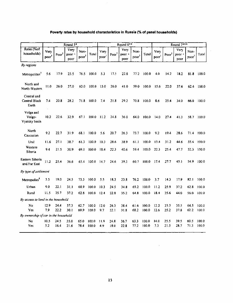
Poverty rates by household characteristics in Russia (% of panel households)

Round 5* Round 6** Round 7**lRates (%of r Very Non- ery VeVery Non-households) p Poor2 poor - Total p Poor2 poor+ p 3 Total o Poor2 poor + 3 Total

popoor'o poor 3 poor porpoIor orpopoor~~~~~~~~~~~~~~~~po

By regions

Metropolitan7 5.6 17.9 23.5 76.5 100.0 5.3 17.5 22.8 77.2 100.0 4.0 14.2 18.2 81.8 100.0

North-Westrnd 11.0 26.0 37.0 63.0 100.0 15.0 26.0 41.0 59.0 100.0 15.6 22.0 37.6 62.4 100.0North-Westem

Central andCentral Black 7.4 20.8 28.2 71.8 100.0 7.4 21.8 29.2 70.8 100.0 8.6 25.4 34.0 66.0 100.0

Earth

Volga andVolgo- 10.2 22.6 32.9 67.1 100.0 11.2 24.8 36.0 64.0 100.0 14.0 27.4 41.3 58.7 100.0

Vyatsky basin

Caucasian 9.2 22.7 31.9 68.1 100.0 5.6 20.7 26.3 73.7 100.0 9.2 19.4 28.6 71.4 100.0Caucasian

Ural 11.6 27.1 38.7 61.3 100.0 10.3 28.6 38.9 61.1 100.0 13.4 31.2 44.6 55.4 100.0

Western 9.4 21.5 30.9 69.1 100.0 18.4 22.3 40.6 59.4 100.0 22.3 25.4 47.7 52.3 100.0Siberia

Eastem Siberia 11.2 25.4 36.6 63.4 100.0 14.7 24.6 39.3 60.7 100.0 17.4 27.7 45.1 54.9 100.0and Far East

By type of seltlement

Metropolies8 5.5 19.0 24.5 75.5 100.0 5.5 18.3 23.8 76.2 100.0 3.7 14.3 17.9 82.1 100.0

Urban 9.0 22.1 31.1 68.9 100.0 10.3 24.5 34.8 65.2 100.0 11.2 25.9 37.2 62.8 100.0

Rural 11.5 25.7 37.2 62.8 100.0 12.4 22.8 35.2 64.8 100.0 18.4 25.6 44.0 56.0 100.0

By access to land in the household

No 12.9 24.4 37.3 62.7 100.0 12.0 26.3 38.4 61.6 100.0 12.2 23.3 35.5 64.5 100.0Yes 7.9 22.2 30.1 69.9 100.0 9.7 22.1 31.8 68.2 100.0 12.6 25.2 37.8 62.2 100.0

By ownership of car in the household

No 10.5 24.5 35.0 65.0 100.0 11.9 24.8 36.7 63.3 100.0 14.0 25.5 39.5 60.5 100.0Yes 5.2 16.4 21.6 78.4 100.0 4.9 18.0 22.8 77.2 100.0 7.3 21.5 28.7 71.3 100.0

23

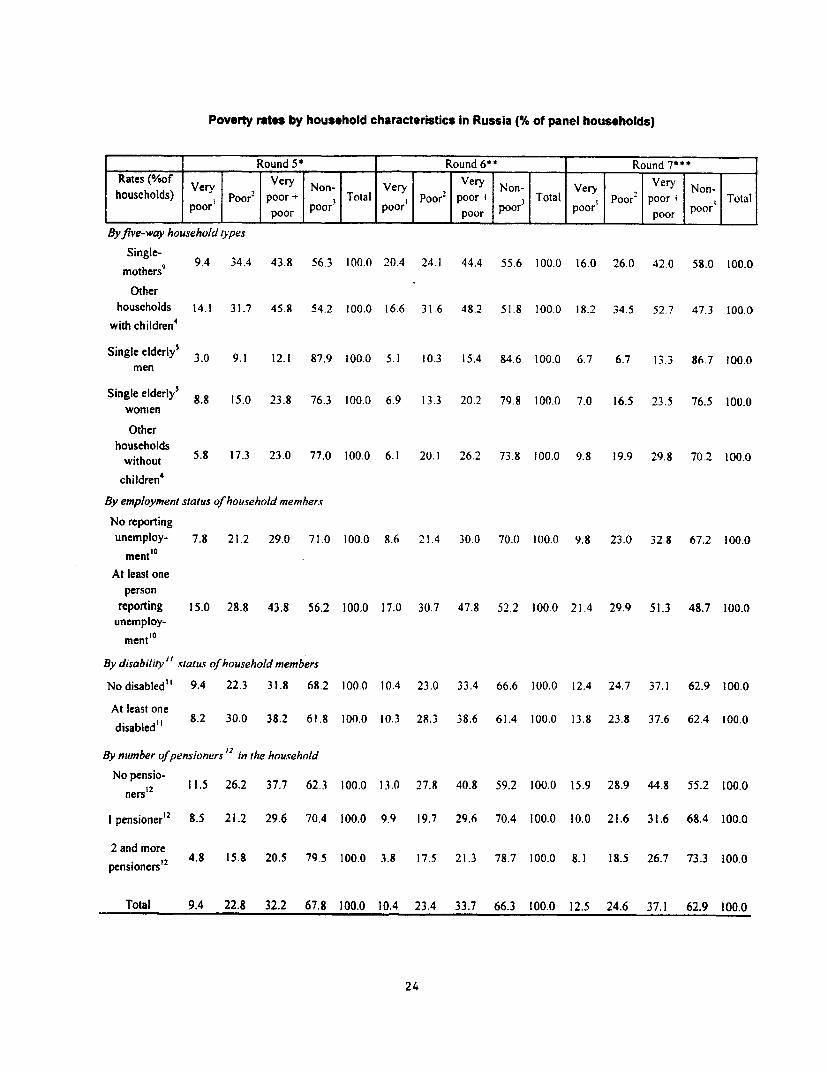
Poverty rates by household characteristics In Russia (% of panel households)

Round 5* Round 6*= Round 7*

Rates Veo y Very tNon-r eyNn Vr eyN,houscholds) Very | p 2 | poor + 00 N Total Very Poorz poor N Total Poor. poor + Total

poor I | poor poor poor poor poor poor' poor poor

Byfwve-way household types

Single-mother9 9.4 34A 43.8 56.3 100.0 20.4 24.1 44.4 55.6 100.0 16.0 26.0 42.0 58.0 100.0

mothere

Otherhouseholds 14.1 31.7 45.8 54.2 100.0 16.6 31.6 48.2 51.8 100.0 18.2 34.5 52.7 47.3 100.0

with children'

Single elderly5 3.0 9.1 12.1 87.9 100.0 5.1 10.3 15.4 84.6 100.0 6.7 6.7 13.3 86.7 100.0men

Single elderlys 8.8 15.0 23.8 76.3 100.0 6.9 13.3 20.2 79.8 100.0 7.0 16.5 23.5 76.5 100.0

women

Otherhouseholds

without 5.8 17.3 23.0 77.0 100.0 6.1 20.1 26.2 73.8 100.0 9.8 19.9 29.8 70.2 100.0

children'

By employment status ofhousehold members

No reportingunemploy- 7.8 21.2 29.0 71.0 100.0 8.6 21.4 30.0 70.0 100.0 9.8 23.0 32.8 67.2 100.0

ment'°

At least oneperson

reporting 15.0 28.8 43.8 56.2 100.0 17.0 30.7 47.8 52.2 100.0 21.4 29.9 51.3 48.7 100.0unemploy-

ment'°

By disability" status of household nmembers

Nodisabled" 9.4 22.3 31.8 68.2 100.0 10.4 23.0 33.4 66.6 100.0 12.4 24.7 37.1 62.9 100.0

At least onedisabled" 8.2 30.0 38.2 61.8 100.0 10.3 28.3 38.6 61.4 100.0 13.8 23.8 37.6 62.4 100.0

By number ofpensioners 2 in the household

No pensio-ners12 11.5 26.2 37.7 62.3 100.0 13.0( 27.8 40.8 59.2 100.0 15.9 28.9 44.8 55.2 100.0

I pensioner12 8.5 21.2 29.6 70.4 100.0 9.9 19.7 29.6 70.4 100.0 10.0 21.6 31.6 68.4 100.0

2 and morepensioners'2 4.8 15.8 20.5 79.5 100.0 3.8 17.5 21.3 78.7 100.0 8.1 18.5 26.7 73.3 100.0

Total 9.4 22.8 32.2 67.8 100.0 10.4 23.4 33.7 66.3 100.0 12.5 24.6 37.1 62.9 100.0

24

Poverty rates by household characteristics in Russia (% of panel households)

Round 5 of the RLMS survey was conducted in Russia in November 1994 - January 1995** Round 6 of the RLMS survey was conducted in Russia in October - November 1995* Round 7 of the RLMS survey was conducted in Russia in October - December 1996

Very poor - households with total expenditures (see explanation in # 13) below 50% of the official regionallyI differentiated (see explanation in # 14) subsistence minimum adjusted for economies of scale in the household

(Ministry of Labour of Russia)

Poor - households with total expenditures (see explanation in # 13) below official regionally differentiated (see2 explanation in # 14) subsistence minimum adjusted for economies of scale in the houschold (Ministry of Labour of

Russia)Non-poor - households with total expenditures (see explanation in # I 3) above or equal to official regionally

3 differentiated (see explanation in # 14) subsistence minimum adjusted for economies of scale in the household(Ministry of Labour of Russia)

4 Children - those below 14 years of age

5 Elderly - men above 59 and women above 54 years of age6 Household head - as defined by UNC7 Metropolitan - Moscow and Moscow region (oblast), St. Petersburg and Leningradski region (oblast)

8 Metropolies - Moscow and St. Petersburg9Single mothers - a category choscn instead of single parent since there was only I case of single father in the sample

as of round 7 and no such cases as of rounds 5 and 610 Reporting unemployment - those who do not report any work, receive neither pension nor disability benefit and

11 Disabled - those who receive disability benefit

12 Pensioners - those who reccive old-age and/or early retirement pension

13 Total expenditures - total household monetary food and non-food expenditures excluding big purchases, purchases of14 Regionally differentiated subsistence miniitim - 8 regional poverty lines computed as population weighted average

25

Poverty composition by household chAracteristics in Russia (% of panel households)

Round 5* Round 6** Round 7***

Compousitionldso Verypo |Poor2 Non-poor3 Total Very poor' Poor2 Non-poor3 Total Very poor' Poor2 Non-poor' Total

By household size

1 15.4 10.9 19.1 16.9 12.0 10.3 22.1 18.3 13.0 10.7 23.4 19.02 14.9 18,6 34.0 28.7 12.4 21.6 32.0 27.5 16.8 20.7 31.8 27.23 19.5 24.2 22.8 22.8 25.8 24.1 21.8 22.7 23.9 26.9 20.7 22.64 27.8 32.0 16.6 21.1 26.6 29.3 16.8 20.7 27.0 26.5 16.4 20.2

5 and more 22.4 14.3 7.6 10.5 23.2 14.6 7.4 10.7 19.3 15.2 7.7 11.0Total 100.0 100.0 100.0 100.0 100.0 100.0 100.0 100.0 100.0 100.0 100.0 100.0

By number of children in the household

Nochildren4 40.2 43.3 67.5 59.4 36.7 47.8 69.3 60.9 45.0 47.4 71.1 62.0I child4 27.4 32.0 23.0 25.5 34.1 30.4 21.6 25.0 30.7 33.2 20.7 25.0

2children andmore 32.4 24.7 9.5 15.1 29.2 21.8 9.1 14.1 A 19.4 8.2 13.0Total 100.0 100.0 100.0 100.0 100.0 100.0 100.0 100.0 100.0 100.0 100.0 100.0

c°' By number of elderly5 in the household

No iderly5 58.1 60.3 48.4 52.0 60.3 59.9 45.5 50.4 57.8 58.0 44.4 49.4I elderly5 32.4 29.1 31.3 30.9 33.0 28.3 33.4 32.2 29.2 29.9 35.4 33.3

2 and more elderly5 9.5 10.6 20.3 17.1 6.7 11.8 21.1 17.4 13.0 12.2 20.2 17.3Total 100.0 100.0 100.0 100.0 100.0 100.0 100.0 100.0 100.0 100.0 100.0 100.0

Byfour-*ypefamily composition

No children4, no elderly' 11.2 17.4 23.1 20.7 15.7 18.1 21.8 20.3 16.8 18.3 22.4 20.7Children4, no elderly5 46.9 42.9 25.3 31.3 44.6 41.8 23.7 30.1 41.0 39.7 21.9 28.7Elderly3 , no children4 29.0 25.9 44.4 38.7 21.0 29.6 47.4 40.5 28.3 29.1 48.6 41.3

Children4 and elderly5 12.9 13.8 7.2 9.2 18.7 10.5 7.0 9.1 14.0 13.0 7.0 9.3Total 100.0 100.0 100.0 100.0 100.0 100.0 100.0 100.0 100.0 100.0 100.0 100.0

By gender of household head 6Female 22.8 22.3 25.1 24.3 25.8 20.8 26.7 25.2 23.9 19.9 28.6 25.8Male 77.2 77.7 74.9 75.7 74.2 79.2 73.3 74.8 76.1 80.1 71.4 74.2Total 100.0 100.0 100.0 100.0 100.0 100.0 100.0 100.0 100.0 100.0 100.0 100.0

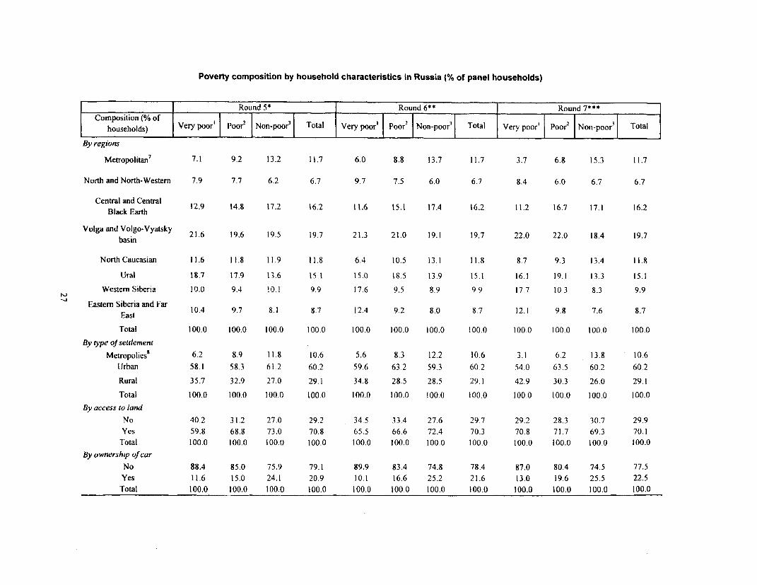
Poverty composition by household characteristics in Russia (% of panel households)

Round 5* Round 6** Round 7***

Composition (% of V 2 3

households) Very pr oPoorf Non-poor3 Total Very poor' Poor' Non-poor' Total Very poor' poor2 Non-poor) Total

By regions

Metropolitan7 7.1 9.2 13.2 11.7 6.0 8.8 13.7 11.7 3.7 6.8 15.3 11.7

North and North-Western 7.9 7.7 6.2 6.7 9.7 7.5 6.0 6.7 8.4 6.0 6.7 6.7

CentralandCentral 12.9 14.S 17.2 16.2 11.6 15.1 17.4 16.2 11.2 16.7 17.1 16.2

Black Earth

Volgaand Volgo-Vyatsky 21.6 19.6 19.5 19.7 21.3 21.0 19.1 19.7 22.0 22.0 18.4 19.7

basin

North Caucasian 11.6 11.8 11.9 11.8 6.4 10.5 13.1 11.8 8.7 9.3 13.4 11.8

Ural 18.7 17.9 13.6 15.1 15.0 18.5 13.9 15.1 16.1 19.1 13.3 15.1

WestemrSiberia 10.0 9.4 10.1 9.9 17.6 9.5 8.9 9.9 17.7 10.3 8.3 9.9

Eastern Siberia and FarEasEmSibeiast dF 10.4 9.7 8.1 8.7 12.4 9.2 8.0 8.7 12.1 9.8 7.6 8.7

Total 100.0 100.0 100.0 100.0 100.0 100.0 100.0 100.0 100.0 100.0 100.0 100.0

By type of settlement

Metropolies" 6.2 8.9 11.8 10.6 5.6 8.3 12.2 10.6 3.1 6.2 13.8 10.6

llrban 58.1 58.3 61 2 60.2 59.6 63.2 59.3 60 2 54.0 63.5 60.2 60.2

Rural 35.7 32.9 27.0 29.1 34.8 28.5 28.5 29.1 42.9 30.3 26.0 29.1

Total 100.0 100.0 100.0 100.0 100.0 100.0 100.0 100.0 100.0 100.0 100.0 100.0

By access to land

No 40.2 31.2 27.0 29.2 34.5 33.4 27.6 29.7 29.2 28.3 30.7 29.9

Ycs 59.8 68.8 73.0 70.8 65.5 66.6 72.4 70.3 70.8 71.7 69.3 70.1

Total 100.0 100.0 100.0 100.0 100.0 100.0 100.0 100.0 100.0 100.0 100.0 100.0

By ownership of car

No 88.4 85.0 75.9 79.1 89.9 83.4 74.8 78.4 87.0 80.4 74.5 77.5

Yes 11.6 15.0 24.1 20.9 10.1 16.6 25.2 21.6 13.0 19.6 25.5 22.5

Total 100.0 100.0 100.0 100.0 100.0 100.0 100.0 100.0 100.0 100.0 100.0 100.0

Poverty composition by household characteristics in Russia (% of panel households)

Round 5* Round 6** Round 7**Composition (Y; of Very poor' | poor2 I Non-poor' Total Very poor' poor 2 Non-poor3 Total Very poorI Poor2 Non-poor' Total

houweholds) Vr

Byfive-way household types

Single-mothers9 2.5 3.7 2.1 2.5 4.1 2.2 1.8 2.1 2.5 2.1 1.8 1.9

Other households withOtherhoushldr w 57.3 53.0 30.4 38.1 59.2 50.1 29.0 37.0 52.5 50.6 27.1 36.1children4

Single elderly' men 0.4 0.5 1.7 1.3 0.7 0.7 1.9 1.5 0.9 0.5 2.4 1.7

Singleelderly'women 11.6 8.2 14.0 12.4 9.0 7.7 16.2 13.5 7.8 9.3 16.9 13.9

Other housetolds without 28.2 34.6 51.9 45.7 27.0 39.4 51.1 45.9 36.3 37.6 51.8 46.4childrn4

Total 100.0 100.0 100.0 100.0 100.0 100.0 100.0 100.0 100.0 100.0 100.0 100.0By employueni status

No repofting uneniploy-op tiuo 65.6 72.7 82.1 78.4 65.5 72.4 83.5 79.0 60.2 71.7 82.0 76.8

S ~~~ment'At least one personreportingunemploy- 34.4 27.3 17.9 21.6 34.5 27.6 16.5 21.0 39.8 28.3 18.0 23.2

ment'°Total 100.0 100.0 100.0 100.0 100.0 100.0 100.0 100.0 100.0 100.0 100.0 100.0

By disability" 1 status of household members

Nodisabled" 94.2 91.3 94.0 93.4 92.9 91.3 93.4 92.8 91.9 92.9 92.7 92.7

Atleastoncdisabled" 5.8 8.7 6.0 6.6 7.1 8.7 6.6 7.2 8.1 7.1 7.3 7.3Total 100.0 100.0 100.0 100.0 100.0 100.0 100.0 100.0 100.0 100.0 100.0 100.0

By number of pensioners 12 in the household

No pensioners"2 62.2 58.4 46.7 50.8 62.5 59.4 44.5 49.9 61.5 57.0 42.6 48.5

I pensioner'2 29.0 29.8 33.4 32.1 31.1 27.5 34.7 32.6 27.0 29.7 36.8 33.8

2and more pensioners'2 8.7 11.8 19.9 17.0 6.4 13.1 20.8 17.5 11.5 13.3 20.6 17.6

Total 100.0 100.0 100.0 100.0 100.0 100.0 100.0 100.0 100.0 100.0 100.0 100.0

Poverty composition by household characteristics in Russia (% of panel households)

* Round 5 of the RLMS survey was conducted in Russia in Novembcr 1994 - January 1995** Round 6 of the RLMS survey was conducted in Russia in October - November 1995

-* Round 7 of the RLMS survey was conducted in Russia in October - December 1996I Very poor - houscholds with total expenditures (see explanation in # 13) below 50% of the official regionally differentiated (see explanation

in # 14) subsistence minimum adjusted for economies of scale in thc household (Ministry of Labour of Russia)

2 Poor - households with total expenditures (see explanation in # 13) below official regionally-differentiated (see explanation in 4 14)

subsistence minimum adjusted for economies of scale in the household (Ministry of Labour of Russia)

3 Non-poor - households with total expenditures (see explanation in 4 13) above or equal to official regionally differentiated (see explanation

in # 14) subsistence minimum adjusted for economies of scale in the household (Ministry of Labour of Russia)

4 Children - those below 14 years of age5 Elderly - men above 59 and women above 54 years of age6 Household head - as defined by UNC

7 Metropolitan - Moscow and Moscow region (oblast), St. Petersburg and Leningradski region (oblast)

8 Metropolies - Moscow and St. Petersburg9 Single mothers - a category chosen instead of singlc parent since there was only 1 case of single father in the sample as of round 7 and no

such cases as of rounds 5 and 610 Reporting unemployment - those who do not report any work, receive neither pension nor disability benefit and would like to work

II Disabled - those who receive disability benefit

12 Pcnsioners - those who receive old-age and/or early retirement pension

13 Total expenditures - total household monetary food and non-food expenditurcs cxcluding big purchases, purchases of luxury goods,bonds/stocks and savings plus value of home-produced food evaluated at prevailing market prices

14 Regionally differentiated subsistence minimum - 8 regional poverty lines computed as population weighted average across 78 officialregional subsistence minima so that to match survey sampie division of Russia into 8 regions

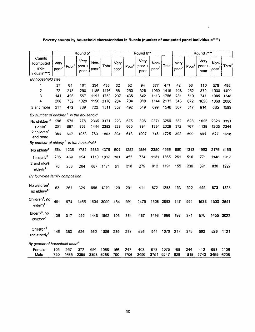
Poverty counts by household characteristics in Russia (number of computed panel individuals")

Round 5* Round 6** Round 7***CountsVeyer

(computed Very Very Non- Very Very Non- Very Very Non-indi- poor' Poor poor + Total p Poor poor + poor3 Total p Poor' poor + Total

viduals*~~~~) Poor poor poor' poor poor' poor'

By household size

1 37 64 101 334 435 32 62 94 377 471 42 68 110 378 4882 72 218 290 1186 1476 66 260 326 1090 1416 108 262 370 1030 14003 141 426 567 1191 1758 207 435 642 1113 1755 231 510 741 1005 17464 268 752 1020 1156 2176 284 704 988 1144 2132 348 672 1020 1060 2080

5 and more 317 472 789 722 1511 357 492 849 699 1548 367 547 914 685 1599

By number of children4 in the household

No children4 198 578 776 2395 3171 223 675 898 2371 3269 332 693 1025 2326 33511 child4 251 687 938 1444 2382 329 665 994 1334 2328 372 767 1139 1205 2344

2 children4 386 667 1053 750 1803 394 613 1007 718 1725 392 599 991 627 1618and more

By number of elderly 5 in the household

No elderly5 554 1235 1789 2589 4378 604 1282 1886 2380 4266 680 1313 1993 2176 4169

1 elderly5 205 489 694 1113 1807 281 453 734 1131 1865 261 510 771 1146 1917

eadeorl5 76 208 284 887 1171 61 218 279 912 1191 155 236 391 836 1227elderly5

By four-type family composition

N children4, 63 261 324 955 1279 120 291 411 872 1283 133 322 455 873 1328no elderly5

no 491 974 1465 1634 3099 484 991 1475 1508 2983 547 991 1538 1303 2841elderlys

Elderly, 135 317 452 1440 1892 103 384 487 1499 1986 199 371 570 1453 2023children4

Children 4

and elderly5 146 380 526 560 1086 239 287 526 544 1070 217 375 592 529 1121

By gender of household head 6

Female 105 267 372 696 1068 156 247 403 672 1075 168 244 412 693 1105Male 730 1665 2395 3893 6288 790 1706 2496 3751 6247 928 1815 2743 3465 6208

30

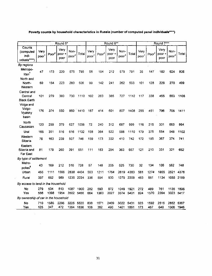
Poverty counts by household characteristics in Russia (number of computed panel individuals-^^)

Round 5- Round 6*| Round 7***Counts VrV

(computed Very Very Non- Very Very Non- Very Very Non-di- poor poor2 poor + p Total 1 poor2 poor + 3 Total Io1 poor2 poor + p Total

viduals**) poor poor poor poor poor poor poor poor-

By regions

litrop7 47 173 220 575 795 58 154 212 579 791 35 147 182 624 806litan7

North andNorth- 69 154 223 283 506 99 142 241 262 503 101 128 229 270 499

WesternCentral and

Central 101 279 380 730 1110 102 283 385 727 1112 117 338 455 653 1108Black EarthVolga and

Vyoltok 176 374 550 860 1410 187 414 601 807 1408 255 451 706 705 1411basin

Caucasia 120 259 379 627 1006 72 240 312 687 999 116 215 331 663 994Caucasian

Ural 165 351 516 616 1132 158 364 522 588 1110 179 375 554 548 1102

Western 76 163 239 507 746 159 173 332 410 742 172 195 367 374 741Siberia

EasternSiberiaand 81 179 260 391 651 111 183 294 363 657 121 210 331 321 652

Far EastBy type of settlement

Metro- 43 169 212 516 728 57 148 205 525 730 32 134 166 582 748polies 4Urban 455 1111 1566 2838 4404 553 1211 1764 2619 4383 581 1274 1855 2521 4376

Rural 337 652 989 1235 2224 336 594 930 1279 2209 483 651 1134 1055 2189

By access to land in the household

No 279 534 813 1087 1900 282 590 872 1049 1921 272 489 761 1135 1896Yes 556 1398 1954 3502 5456 664 1363 2027 3374 5401 824 1570 2394 3023 5417

By ownership of car in the household

No 710 1585 2295 3225 5520 838 1571 2409 3022 5431 923 1592 2515 2852 5367Yes 125 347 472 1364 1836 108 382 490 1401 1891 173 467 640 1306 1946

31

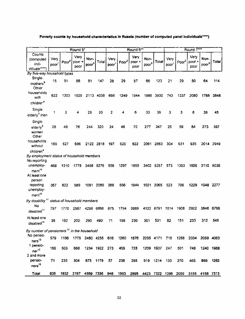
Poverty counts by household characteristics In Russia (number of computed panel individuals7)

__________ Round 5- Round 6- Round 7***

Counts Vr eyNn(computed Very Very Non- Very Very Non- Very Very Non-

ndi- poor' Poor2 poor + 3 Total Poor2 poor + 3 Total , poor2 poor +Po Total

viduals"*^) poor poor poor poor poor poor poor poorBy five-way household types

mother9 15 51 66 81 147 28 29 57 66 123 21 29 50 64 114mothers9

Otherhouseholds

with 622 1303 1925 2113 4038 695 1249 1944 1986 3930 743 1337 2080 1768 3848

children4

Single 1 3 4 29 33 2 4 6 33 39 3 3 6 39 45elderly5 men

Single

elderly5 28 48 76 244 320 24 46 70 277 347 25 59 84 273 357womenOther

householdswithout 169 527 696 2122 2818 197 625 822 2061 2883 304 631 935 2014 2949

children4

By employment status of household membersNo reportingunemploy- 468 1310 1778 3498 5276 558 1297 1855 3402 5257 573 1353 1926 3110 5036

ment'°At least one

personreporting 367 622 989 1091 2080 388 656 1044 1021 2065 523 706 1229 1048 2277

unemploy-

mentl°

By disability " status of household membersNod l 797 1770 2567 4299 6866 875 1794 2669 4122 6791 1014 1908 2922 3846 6768

disableda

dAtbledso1 38 162 200 290 490 71 159 230 301 531 82 151 233 312 545disabled"

By number of pensioners 12 in the householdNo pensio-ners 1

2 579 1196 1775 2480 4255 616 1260 1876 2295 4171 716 1288 2004 2059 4063

1 pensio-ner 12 185 503 688 1234 1922 273 455 728 1209 1937 247 501 748 1240 1988

2 and morepensio- 71 233 304 875 1179 57 238 295 919 1214 133 270 403 859 1262ners 12

Total 835 1932 2767 4589 7356 946 1953 2899 4423 7322 1096 2059 3155 4158 7313

32

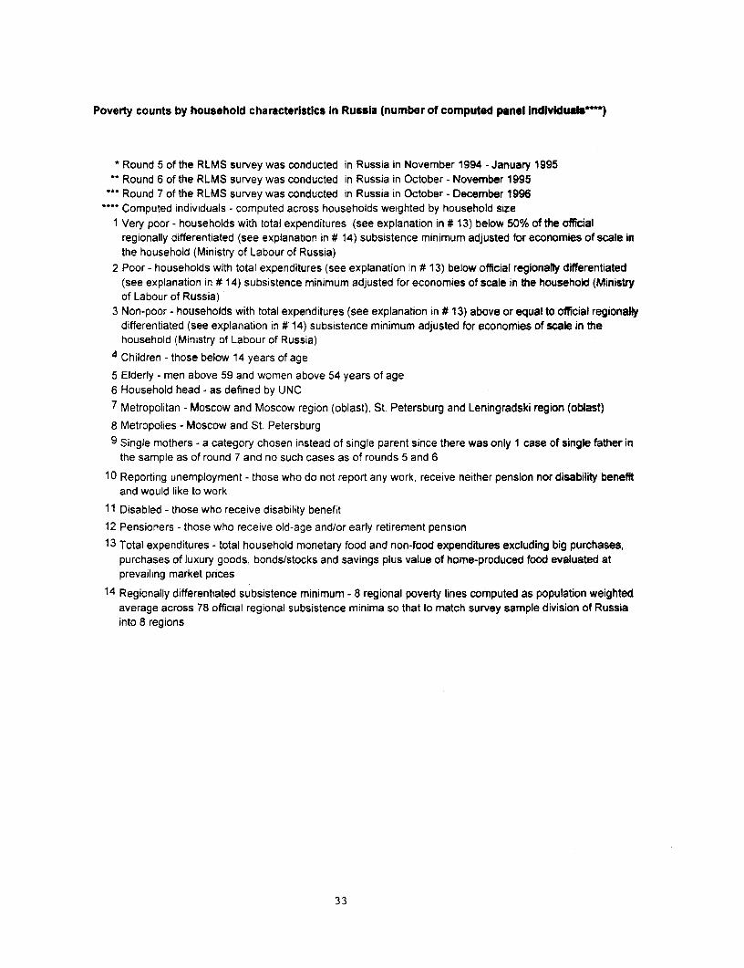
Poverty counts by household characteristics in Russia (number of computed panel indiv1duabl )

* Round 5 of the RLMS survey was conducted in Russia in November 1994 -January 1995Round 6 of the RLMS survey was conducted in Russia in October - November 1995Round 7 of the RLMS survey was conducted in Russia in October - December 1996Computed individuals - computed across households weighted by household size

1 Very poor - households with total expenditures (see explanation in # 13) below 50% of the officialregionally differentiated (see explanation in # 14) subsistence minimum adjusted for economies of scale inthe household (Ministry of Labour of Russia)

2 Poor - households with total expenditures (see explanation in # 13) below official regionally differentiated(see explanation in # 14) subsistence minimum adjusted for economies of scale in the household (Ministryof Labour of Russia)

3 Non-poor - households with total expenditures (see explanation in # 13) above or equal to official regionallydifferentiated (see explanation in #'14) subsistence minimum adjusted for economies of scale in thehousehold (Ministry of Labour of Russia)

4 Children - those below 14 years of age

5 Elderly - men above 59 and women above 54 years of age6 Household head - as defined by UNC

7 Metropolitan - Moscow and Moscow region (oblast), St. Petersburg and Leningradski region (oblast)8 Metropolies - Moscow and St. Petersburg

9 Single mothers - a category chosen instead of single parent since there was only 1 case of single father inthe sample as of round 7 and no such cases as of rounds 5 and 6

10 Reporting unemployment - those who do not report any work, receive neither pension nor disability benefitand would like to work

11 Disabled - those who receive disability benefit12 Pensioners - those who receive old-age and/or early retirement pension

13 Total expenditures - total household monetary food and non-food expenditures excluding big purchases,purchases of luxury goods, bonds/stocks and savings plus value of home-produced food evaluated atprevailing market prices

14 Regionally differentiated subsistence minimum - 8 regional poverty lines computed as population weightedaverage across 78 official regional subsistence minima so that to match survey sample division of Russiainto 8 regions

33

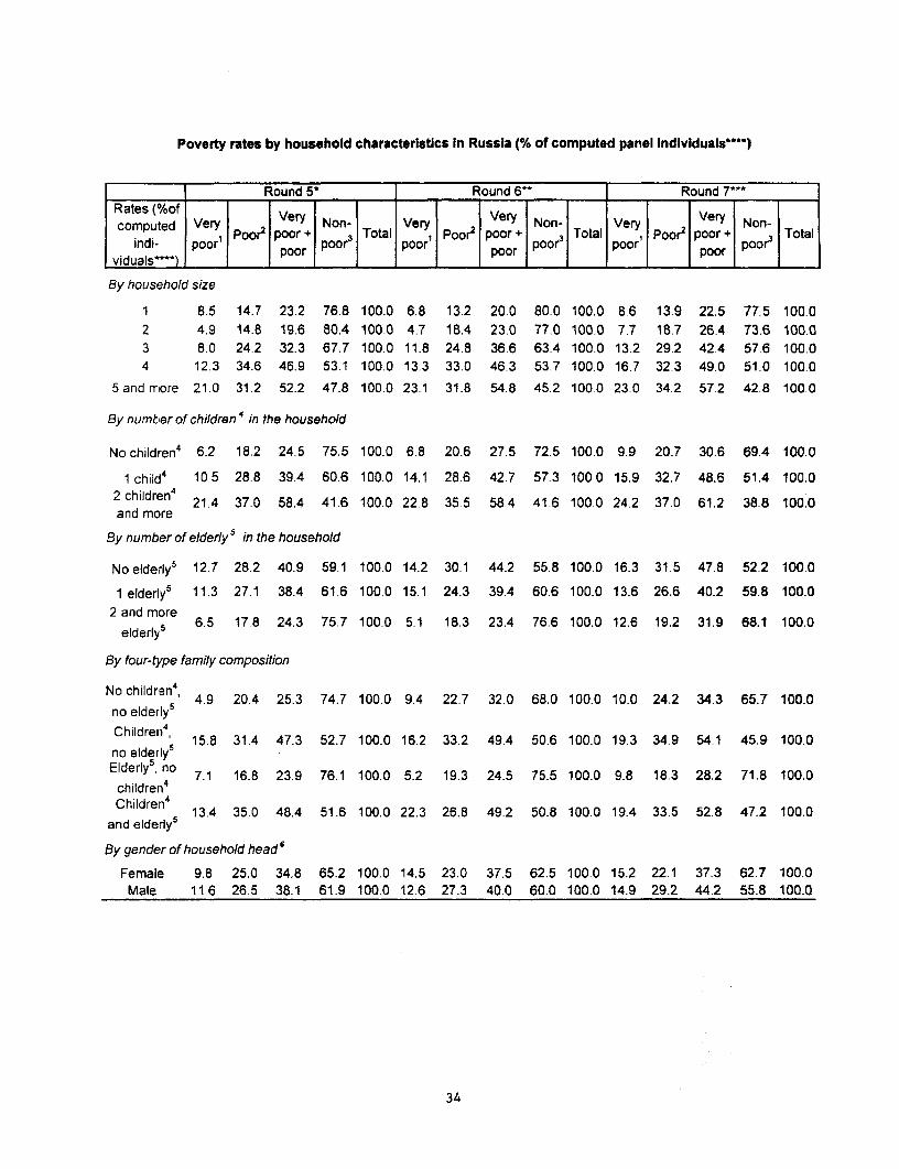
Poverty rates by household characteristics in Russia (% of computed panel individuals*")

Round 5' Round 6- Round 7**_Rates (%of VrVeyVercomputed Very Very Non- Vs Very Non- Very ery Non-

indi- poor' Poor poor+ poor3 Total poor' oor + poor tal poor' Poor' poor + poor Totalviduals'***) poor poor poor

By household size

1 8.5 14.7 23.2 76.8 100.0 6.8 13.2 20.0 80.0 100.0 8.6 13.9 22.5 77.5 100.02 4.9 14.8 19.6 80.4 100.0 4.7 18.4 23.0 77.0 100.0 7.7 18.7 26.4 73.6 100.03 8.0 24.2 32.3 67.7 100.0 11.8 24.8 36.6 63.4 100.0 13.2 29.2 42.4 57.6 100.04 12.3 34.6 46.9 53.1 100.0 13.3 33.0 46.3 53.7 100.0 16.7 32.3 49.0 51.0 100.0

5 and more 21.0 31.2 52.2 47.8 100.0 23.1 31.8 54.8 45.2 100.0 23.0 34.2 57.2 42.8 100.0

By number of children 4 in the household

No children4 6.2 18.2 24.5 75.5 100.0 6.8 20.6 27.5 72.5 100.0 9.9 20.7 30.6 69.4 100.0

1 child4 10.5 28.8 39.4 60.6 100.0 14.1 28.6 42.7 57.3 100.0 15.9 32.7 48.6 51.4 100.0

2 children' 21.4 37.0 58.4 41.6 100.0 22.8 35.5 58.4 41.6 100.0 24.2 37.0 61.2 38.8 100.0and more

By number of elderly 5 in the household

No elderly' 12.7 28.2 40.9 59.1 100.0 14.2 30.1 44.2 55.8 100.0 16.3 31.5 47.8 52.2 100.0

1 elderlys 11.3 27.1 38.4 616 100.0 15.1 24.3 39.4 60.6 100.0 13.6 26.6 40.2 59.8 100.0

2 6.5 17.8 24.3 75.7 100.0 5.1 18.3 23.4 76.6 100.0 12.6 19.2 31.9 68.1 100.0elderly5

By four-type family composition

No children', 4.9 20.4 25.3 74.7 100.0 9.4 22.7 32.0 68.0 100.0 10.0 24.2 34.3 65.7 100.0no elderly 5

Children'4, 15.8 31.4 47.3 52.7 100.0 16.2 33.2 49.4 50.6 100.0 19.3 34.9 54.1 45.9 100.0no elderly5

Ery 7.1 16.8 23.9 76.1 100.0 5.2 19.3 24.5 75.5 100.0 9.8 18.3 28.2 71.8 100.0children'Children' 13.4 35.0 48.4 51.6 100.0 22.3 26.8 49.2 50.8 100.0 19.4 33.5 52.8 47.2 100.0

and elderly5

By gender of household head 6

Female 9.8 25.0 34.8 65.2 100.0 14.5 23.0 37.5 62.5 100.0 15.2 22.1 37.3 62.7 100.0Male 11.6 26.5 38.1 61.9 100.0 12.6 27.3 40.0 60.0 100.0 14.9 29.2 44.2 55.8 100.0

34

Poverty rates by household characteristics in Russia (% of computed panel individuals*")

Round 5| Round 6** Round 7-Rates (%of Vcomputed Very Very Non- Very Very Non- Very Very Non-

.iduals~) poor1 Poor2 poor + Total p Poor2 poor + p Total p Poor2 poor + p Totlindi- poor poor poor poor

By regions

Metropo- 5.9 21.8 27.7 72.3 100.0 7.3 19.5 26.8 73.2 100.0 4.3 18.2 22.6 77.4 100.0litan7

North andNorth- 13.6 30.4 44.1 55.9 100.0 19.7 28.2 47 9 52.1 100.0 20.2 25.7 45.9 54.1 100.0

Western

Central andCentral 9 1 25.1 34.2 65.8 100.0 9.2 25.4 34.6 65.4 100.0 10.6 305 41.1 58.9 100.0

Black Earth

Volga and

Volgo- 12.5 26.5 39.0 61.0 100.0 13.3 29.4 42.7 57.3 100.0 18.1 32.0 50.0 50.0 100.0Vyatsky

basin

North 11.9 25.7 37.7 62.3 100.0 7.2 24 0 312 68 8 100.0 11.7 21.6 33.3 66.7 100.0Ca3ucasian

Ural 14.6 31.0 45.6 54.4 100.0 14.2 32.8 47.0 53.0 100.0 16.2 34.0 50.3 49.7 100.0

Western 10.2 21.8 32.0 68.0 100.0 21.4 23.3 44.7 55.3 100.0 23.2 26.3 49.5 50.5 100.0Siberia

EastemSiberia and 12.4 27.5 39.9 60.1 100.0 16.9 27.9 44.7 55 3 100.0 18.6 32.2 50.8 49.2 100.0

Far East

By type of settlementMetro-polies8 5.9 23.2 29.1 70.9 100.0 7.8 20.3 28.1 71.9 100.0 4.3 17.9 22.2 77.8 100.0

Urban 10.3 25.2 35.6 64.4 100.0 12.6 27.6 40.2 59.8 100.0 13.3 29.1 42.4 57.6 100.0

Rural 15.2 29.3 44.5 55.5 100.0 15.2 26.9 42.1 57.9 100.0 22.1 29.7 51.8 48.2 100.0

By access to land in the householdNo 14.7 28.1 42.8 57.2 100.0 14.7 30.7 45.4 54.6 100.0 14.3 25.8 40.1 59.9 100.0

Yes 10.2 25.6 35.8 64.2 100.0 12.3 25.2 37.5 62.5 100.0 15.2 29.0 44.2 55.8 100.0

By ownership of car in the household

No 12.9 28.7 41.6 58.4 100.0 15.4 28.9 44.4 55.6 100.0 17.2 29.7 46.9 53.1 100.0Yes 6.8 18.9 25.7 74.3 100.0 5.7 20.2 25.9 74.1 100.0 8.9 24.0 32.9 67.1 100.0

35

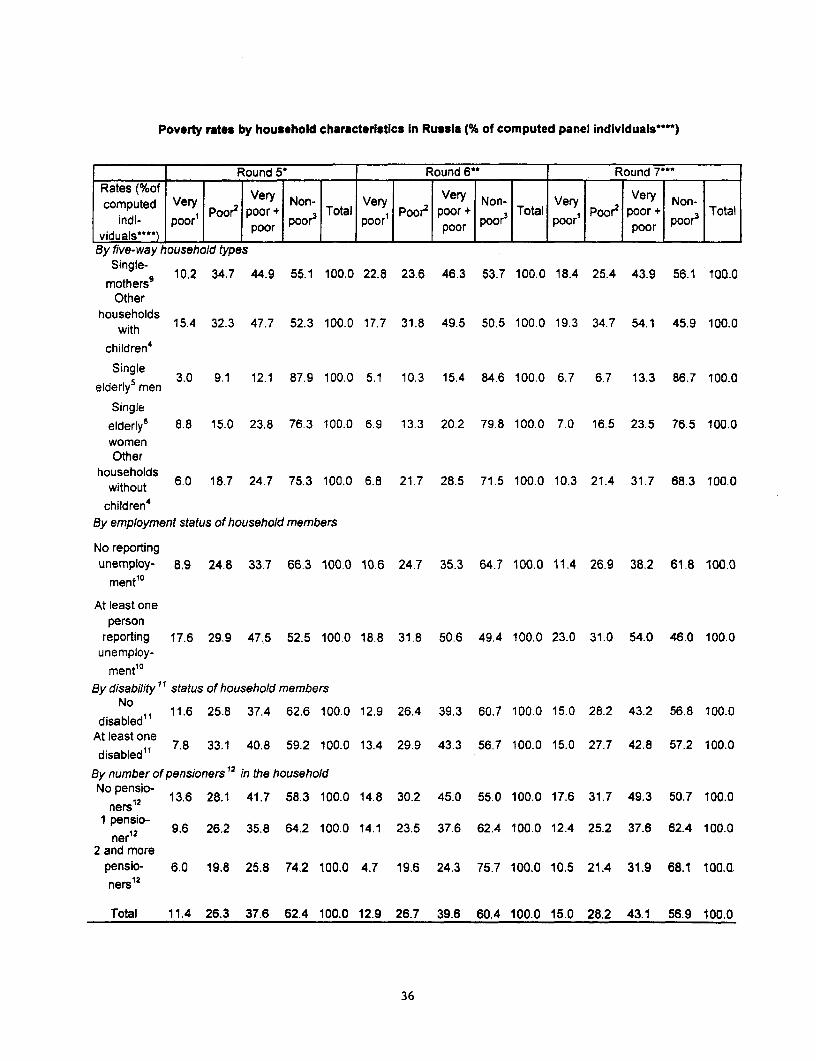
Poverty rates by household characteristics in Russia (% of computed panel individuals***)

Rates ( lofI Round 5* Round 6** Round 7***

computed Very Very Non- Very Very Non- Very Very Non-indi- poor' Poor2 poor + poor3 Total poor'or poor + poor3 Total poor'o poor+ poor+ 3 Total

viduas-) poporprpoor poor po 1 poor po

By five-way household types

mother9 10.2 34.7 44.9 55.1 100.0 22.8 23.6 46.3 53.7 100.0 18.4 25.4 43.9 56.1 100.0rnothers9

Otherhouseholds

with 15.4 32.3 47.7 52.3 100.0 17.7 31.8 49.5 50.5 100.0 19.3 34.7 54.1 45.9 100.0children4

Single 3.0 9.1 12.1 87.9 100.0 5.1 10.3 15.4 84.6 100.0 6.7 6.7 13.3 86.7 100.0elderly5 men

Singleelderly5 8.8 15.0 23.8 76.3 100.0 6.9 13.3 20.2 79.8 100.0 7.0 16.5 23.5 76.5 100.0womenOther

wsithout 6.0 18.7 24.7 75.3 100.0 6.8 21.7 28.5 71.5 100.0 10.3 21.4 31.7 68.3 100.0children4

By employment status of household members

No reportingunemploy- 8.9 24.8 33.7 66.3 100.0 10.6 24.7 35.3 64.7 100.0 11.4 26.9 38.2 61.8 100.0

ment10

At least oneperson

reporting 17.6 29.9 47.5 52.5 100.0 18.8 31.8 50.6 49.4 100.0 23.0 31.0 54.0 46.0 100.0unemploy-

ment'°By disability " status of household members

Nodisabled1' 11.6 25.8 37.4 62.6 100.0 12.9 26.4 39.3 60.7 100.0 15.0 28.2 43.2 56.8 100.0

At least onedisabled" 7.8 33.1 40.8 59.2 100.0 13.4 29.9 43.3 56.7 100.0 15.0 27.7 42.8 57.2 100.0

By number of pensioners 12 in the household

npes 12 13.6 28.1 41.7 58.3 100.0 14.8 30.2 45.0 55.0 100.0 17.6 31.7 49.3 50.7 100.0ners1

1 e2 9.6 26.2 35.8 64.2 100.0 14.1 23.5 37.6 62.4 100.0 12.4 25.2 37.6 62.4 100.0ner'

2 and morepensio- 6.0 19.8 25.8 74.2 100.0 4.7 19.6 24.3 75.7 100.0 10.5 21.4 31.9 68.1 100.0.ners' 2

Total 11.4 26.3 37.6 62.4 100.0 12.9 26.7 39.6 60.4 100.0 15.0 28.2 43.1 56.9 100.0

36

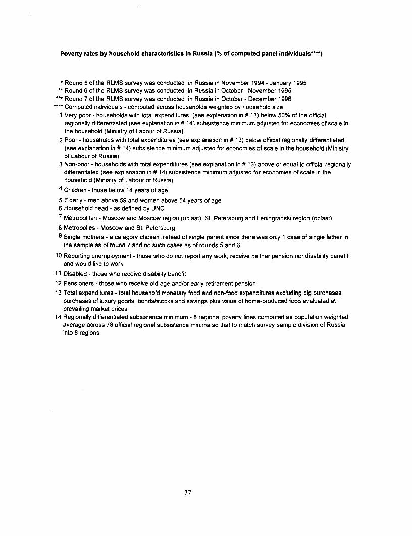
Poverty rates by household characteristics in Russia (% of computed panel individuals^)

Round 5 of the RLMS survey was conducted in Russia in November 1994 - January 1995Round 6 of the RLMS survey was conducted in Russia in October - November 1995Round 7 of the RLMS survey was conducted in Russia in October - December 1996Computed individuals - computed across households weighted by household size

1 Very poor - households with total expenditures (see explanation in # 13) below 50% of the officialregionally differentiated (see explanation in # 14) subsistence minimum adjusted for economies of scale inthe household (Ministry of Labour of Russia)

2 Poor - households with total expenditures (see explanation in # 13) below official regionally differentiated(see explanation in # 14) subsistence minimum adjusted for economies of scale in the household (Ministryof Labour of Russia)

3 Non-poor - households with total expenditures (see explanation in # 13) above or equal to official regionallydifferentiated (see explanation in # 14) subsistence minimum adjusted for economies of scale in thehousehold (Ministry of Labour of Russia)

4 Children - those below 14 years of age5 Elderly - men above 59 and women above 54 years of age6 Household head - as defined by UNC7 Metropolitan - Moscow and Moscow region (oblast), St. Petersburg and Leningradski region (oblast)8 Metropolies - Moscow and St. Petersburg9 Single mothers - a category chosen instead of single parent since there was only 1 case of single father in

the sample as of round 7 and no such cases as of rounds 5 and 6

10 Reporting unemployment - those who do not report any work, receive neither pension nor disability benefitand would like to work

11 Disabled - those who receive disability benefit

12 Pensioners - those who receive old-age and/or early retirement pension13 Total expenditures - total household monetary food and non-food expenditures excluding big purchases,

purchases of luxury goods, bonds/stocks and savings plus value of home-produced food evaluated atprevailing market prices

14 Regionally differentiated subsistence minimum - 8 regional poverty lines computed as population weightedaverage across 78 official regional subsistence minima so that to match survey sample division of Russiainto 8 regions

37

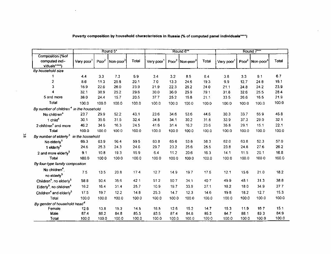
Poverty composition by household characteristics in Russia (% of computed panel individuals****)

Round 5* Round 6** Round 7-Composition (%of

computed indi- Very poor' Poor2 Non-poor3 Total Very poor' Poor2 Non-poor3 Total Very poor' Poor2 Non-poor3 Totalviduals***)

By household size

1 4.4 3.3 7.3 5.9 3.4 3.2 8.5 6.4 3.8 3.3 9.1 6.72 8.6 11.3 25.8 20.1 7.0 13.3 24.6 19.3 9.9 12.7 24.8 19.1

3 16.9 22.0 26.0 23.9 21.9 22.3 25.2 24.0 21.1 24.8 24.2 23.9

4 32.1 38.9 25.2 29.6 30.0 36.0 25.9 29.1 31.8 32.6 25.5 28.45 and more 38.0 24.4 15.7 20.5 37.7 25.2 15.8 21.1 33.5 26.6 16.5 21.9

Total 100.0 100.0 100.0 100.0 100.0 100.0 100.0 100.0 100.0 100.0 100.0 100.0

By number of children4 in the household

No children4 23.7 29.9 52.2 43.1 23.6 34.6 53.6 44.6 30.3 33.7 55 9 45.81 child4 30.1 35.6 31.5 32.4 34.8 34.1 30.2 31.8 33.9 37.3 29.0 32.1

2children 4 andmore 46.2 34.5 16.3 24.5 41.6 31.4 16.2 23.6 35.8 29.1 15.1 22.1Total 100.0 100.0 100.0 100.0 100.0 100.0 100.0 100.0 100.0 100.0 100.0 100.0

co By number of elde ly5 in the household

No elderly5 66.3 63.9 56.4 59.5 63.8 65.6 53.8 58.3 62.0 63.8 52.3 57.0

1 elderly5 24.6 25.3 24.3 24.6 29.7 23.2 25.6 25.5 23.8 24.8 27.6 26.2

2andmoreelderly 5 9.1 10.8 19.3 15.9 6.4 11.2 20.6 16.3 14.1 11.5 20.1 16.8Total 100.0 100.0 100.0 100.0 100.0 100.0 100.0 100.0 100.0 100.0 100.0 100.0

By four-type family composition

Nochildren4 , 7.5 13.5 20.8 17.4 12.7 14.9 19.7 17.5 12.1 15.6 21.0 18.2

no elderly5

Children4 , no elderly5 58.8 50.4 35.6 42.1 51.2 50.7 34.1 407 49.9 48.1 31.3 38.8

Elderly5, no children4 16.2 16.4 31.4 25.7 10.9 19.7 33.9 27.1 18.2 18.0 34.9 27 7

Children4 and elderly5 17.5 19.7 12.2 14.8 25.3 14.7 12.3 14.6 19.8 18.2 12.7 15.3Total 100.0 100.0 100.0 100.0 100.0 100.0 100.0 100.0 100.0 100.0 100.0 100.0

By gender of household head6

Female 12.6 13.8 15.2 14.5 16.5 12.6 15.2 14.7 15.3 11.9 16.7 15.1Male 87.4 86.2 84.8 85.5 83.5 87.4 84.8 85.3 84.7 88.1 83.3 84.9Total 100.0 100.0 100.0 100.0 100.0 100.0 100.0 100.0 100.0 100.0 100.0 100.0

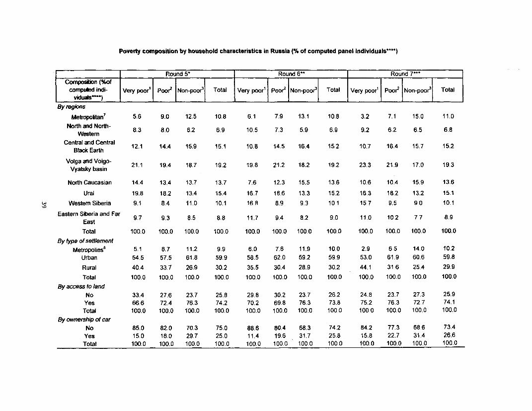
Poverty composition by household characteristics in Russia (% of computed panel individuals****)

Round 5- Round 6** Round 7***Composlion (%of

compuled indi- Very poor' Poor2 Non-poor3 Total Very poor' Poor2 Non-poor3 Total Very poor' Poor2 Non-poor3 Totalviduals)

By regions

Metropolitan7 5.6 9.0 12.5 10.8 6.1 7.9 13.1 10.8 3.2 7.1 15.0 11.0

North and North- 8.3 8.0 6.2 6.9 10.5 7.3 5.9 6.9 9.2 6.2 6.5 6.8WesternCentral and Central 12.1 14.4 15.9 15.1 10.8 14.5 16.4 15.2 10.7 16.4 15.7 15.2

Black Earth

VolgaandVolgo- 21.1 19.4 18.7 19.2 19.8 21.2 18.2 19.2 23.3 21.9 17.0 19.3Vyatsky basin

North Caucasian 14.4 13.4 13.7 13.7 7.6 12.3 15.5 13.6 10.6 10.4 15.9 13.6Ural 19.8 18.2 13.4 15.4 16.7 18.6 13.3 15.2 16.3 18.2 13.2 15.1

W Westem Siberia 9.1 8.4 11.0 10.1 16.8 8.9 9.3 10 1 15-7 9.5 9.0 10.1Eastern Siberia and Far 9.7 9.3 8.5 8.8 11.7 9.4 8.2 9.0 11 0 10.2 7 7 8.9

EastTotal 100.0 100.0 100.0 100.0 100.0 100.0 100.0 100.0 100.0 100.0 100.0 100.0

By type of settlementMetropoliesa 5.1 8.7 11.2 9.9 6.0 7.6 11.9 10.0 2.9 6.5 14.0 10.2

Urban 54.5 57.5 61.8 59.9 58.5 62.0 59.2 59.9 53.0 61.9 60.6 59.8Rural 40.4 33.7 26.9 30.2 35.5 30.4 28.9 30.2 44.1 31 6 25.4 29.9Total 100.0 100.0 100.0 100.0 100.0 100.0 100.0 100.0 100.0 100.0 100.0 100.0

By access to landNo 33.4 27.6 23.7 25.8 29.8 30.2 23.7 26.2 24.8 23.7 27.3 25.9

Yes 66-6 72.4 76.3 74.2 70.2 69.8 76.3 73.8 75.2 76.3 72.7 74.1Total 100.0 100.0 100.0 100.0 100.0 100.0 100.0 100.0 100.0 100.0 100.0 100.0

By ownership of carNo 85.0 82.0 70.3 75.0 88.6 80.4 68.3 74.2 84.2 77.3 68.6 73.4

Yes 15.0 18.0 29.7 25.0 11.4 19.6 31.7 25.8 15.8 22.7 31.4 26.6Total 100.0 100.0 100.0 100.0 100.0 100.0 100.0 100.0 100.0 100.0 100.0 100.0

Poverty composition by household characteristics in Russia (% of computed panel individuals"*)

Round 5* Round 6** Round 7***Composition (%of I

computed indi- Very poor' Poor2 Non-poor3 Total Very poor' Poor3 Non-poor3 Total Very poor' Poor2 Non-poor3 Totalviduals**)

By five-way household types

Single-mothers9 1.8 2.6 1.8 2.0 3.0 1.5 1.5 1.7 1.9 1.4 1.5 1.6

Other households withchildren4 74.5 67.4 46.0 54.9 73.5 64.0 44.9 53.7 67,8 64.9 42.5 52.6

Single elderly5 men 0.1 0.2 0.6 0.4 0.2 0.2 0.7 0.5 0.3 0.1 0.9 0.6

Single elderly5 women 3.4 2.5 5.3 4.4 2.5 2.4 6.3 4.7 2.3 2.9 6 6 4.9Other householdswithout children4 20.2 27.3 46.2 38.3 20.8 32.0 46.6 39.4 27.7 30.6 48.4 40.3

Total 100.0 100.0 100.0 100.0 100.0 100.0 100.0 100.0 100.0 100.0 100.0 100.0By employment status

No reporting unemploy- 56.0 67.8 76.2 71.7 59.0 66.4 76.9 71.8 52.3 65.7 74.8 68.9O ~~mentl°

At least one personreporting unemploy- 44.0 32.2 23.8 28.3 41.0 33.6 23.1 28.2 47.7 34.3 25.2 31.1

mentl°Total 100.0 100.0 100.0 100.0 100.0 100.0 100.0 100.0 100.0 100.0 100.0 100.0

By disability t status of household membersNo disabled" 95.4 91.6 93.7 93.3 92.5 91.9 93.2 92.7 92.5 92.7 92.5 92.5

At least one disabled" 4.6 8.4 6.3 6.7 7.5 8.1 6.8 7.3 7.5 7.3 7.5 7.5

Total 100.0 100.0 100.0 100.0 100.0 100.0 100.0 100.0 100.0 100.0 100.0 100.0By number of pensioners 12 in the household

No pensioners'2 69.3 61.9 54.0 57.8 65.1 64.5 51.9 57.0 65.3 62.6 49.5 55.61 pensioner'2 22.2 26.0 26.9 26.1 28.9 23.3 27.3 26.5 22.5 24.3 29.8 27.22 and more

pensioners12 8.5 12.1 19.1 16.0 6.0 12.2 20.8 16.6 12.1 13.1 20.7 17.3

Total 100.0 100.0 100.0 100.0 100.0 100.0 100.0 100.0 100.0 100.0 100.0 100.0

Poverty composition by household characteristics in Russia (% of computed panel Individuals*"*")

' Round 5 of the RLMS survey was conducted in Russia in November 1994 - January 1995

Round 6 of the RLMS survey was conducted in Russia in October - November 1995

Round 7 of the RLMS survey was conducted in Russia in October - December 1996

Computed individuals - computed across households weighted by household size

1 Very poor - households with total expenditures (see explanation in # 13) below 50% of the official

regionally differentiated (see explanation in # 14) subsistence minimum adjusted for economies of

scale in the household (Ministry of Labour of Russia)

2 Poor - households with total expenditures (see explanation in # 13) below official regionally

differentiated (see explanation in # 14) subsistence minimum adjusted for economies of scale in

the household (Ministry of Labour of Russia)

3 Non-poor - households with total expenditures (see explanation in # 13) above or equal to official

regionally differentiated (see explanation in # 14) subsistence minimum adjusted for economies of

scale in the household (Ministry of Labour of Russia)

4 Children - those below 14 years of age5 Elderly - men above 59 and women above 54 years of age

6 Household head - as defined by UNC7 Metropolitan - Moscow and Moscow region (oblast), St. Petersburg and Leningradski region (oblast)

8 Metropolies - Moscow and St. Petersburg

9 Single mothers - a category chosen instead of single parent since there was only 1 case of single

father in the sample as of round 7 and no such cases as of rounds 5 and 6

10 Reporting unemployment - those who do not report any work, receive neither pension nor

disability benefit and would like to work

11 Disabled - those who receive disability benefit

12 Pensioners - those who receive old-age and/or early retirement pension

13 Total expenditures - total household monetary food and non-food expenditures excluding big purchases,

purchases of luxury goods, bonds/stocks and savings plus value of home-produced food evaluated at

prevailing market prices

14 Regionally differentiated subsistence minimum - 8 regional poverty lines computed as population weighted

average across 78 official regional subsistence minima so that to match survey sample division of Russia

into 8 regions

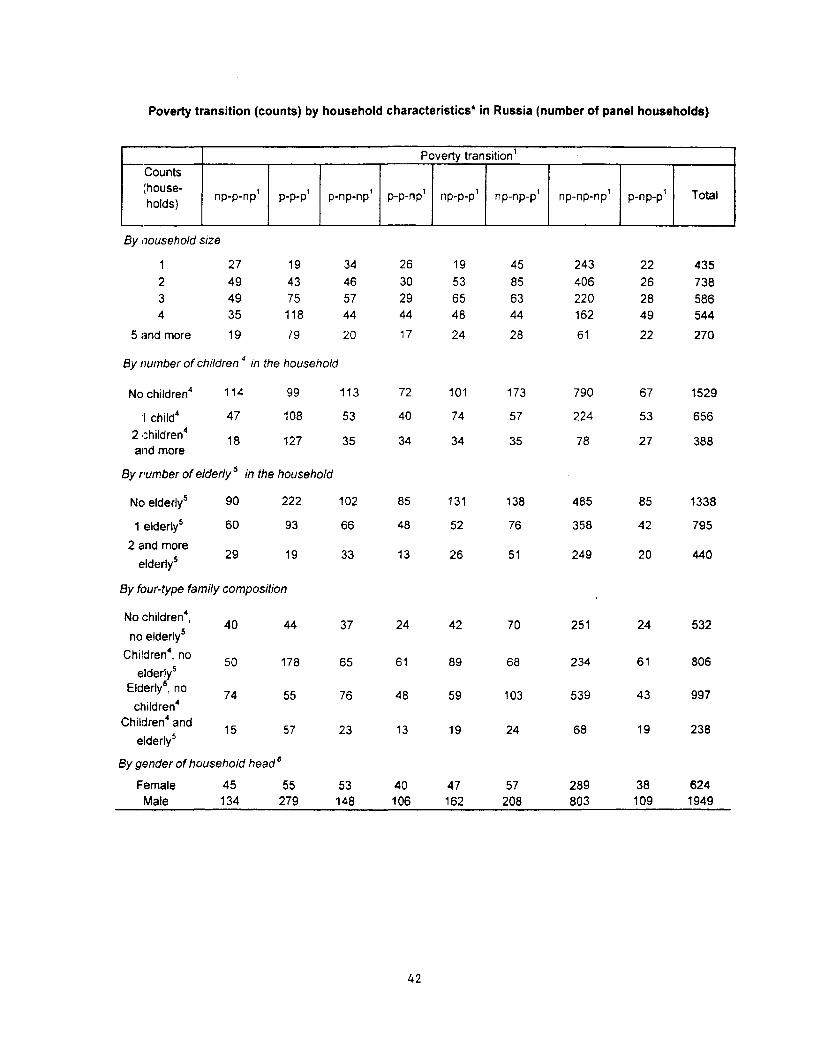
Poverty transition (counts) by household characteristics* in Russia (number of panel households)

Poverty transition'Counts

(house- np-p-np1 p pp' p-np-np' p-p-npl np-p-p1 np-np-p' np-np-npl p-np-p1 Totalholds)

By nousehold size

1 27 19 34 26 19 45 243 22 4352 49 43 46 30 53 85 406 26 7383 49 75 57 29 65 63 220 28 5864 35 118 44 44 48 44 162 49 544

5 and more 19 79 20 17 24 28 61 22 270

By number of children4 in the household

Nochildren4 114 99 113 72 101 173 790 67 1529

I child4 47 108 53 40 74 57 224 53 6562 children4 18 127 35 34 34 35 78 27 388and more

By number of elderly5 in the household

No elderlys 90 222 102 85 131 138 485 85 1338

1 elderly5 60 93 66 48 52 76 358 42 795

2 and moreelderly 5 29 19 33 13 26 51 249 20 440

By four-type family composition

No children, 40 44 37 24 42 70 251 24 532no elderly5

Children4, no 50 178 65 61 89 68 234 61 806

elderly5

Elderly5, no 74 55 76 48 59 103 539 43 997children4

Children4 and 15 57 23 13 19 24 68 19 238elderly6

By gender of household head 6

Female 45 55 53 40 47 57 289 38 624Male 134 279 148 106 162 208 803 109 1949

42

Poverty transition (counts) by household characteristics* in Russia (number of panel households)

Poverty transitionCounts

(hols) np-p-np p-p-p p-np-np p-p-np np-p-p' np-np-p np-np-np p-np-p1 Total

By regions

Metropo- 27 14 27 19 9 21 174 11 302litan7

North andNorth- 15 34 11 11 11 12 71 8 173

WesternCentral and

Central Black 27 50 34 12 33 37 203 22 418Earth

Volga andVolgo-Vyatsky 30 76 32 29 48 56 207 30 508

basin

North 25 19 34 22 14 32 136 22 304Caur,asian

Ural 22 69 27 28 32 46 138 26 388Western 21 37 13 11 35 32 89 18 256SiberiaEastern

Siberia and 12 35 23 14 27 29 74 10 224Far East

By type of settlement

MetropoliesB 24 13 26 19 9 18 155 9 273

Urban 110 206 111 87 136 156 666 78 1550

Rural 45 115 64 40 64 91 271 60 750

By access to land in the household

No 54 117 68 57 58 59 300 38 751Yes 125 217 133 89 151 206 792 109 1822

By ownership of car in the household

No 139 292 162 128 173 211 801 130 2036Yes 40 42 39 18 36 54 291 17 537

43

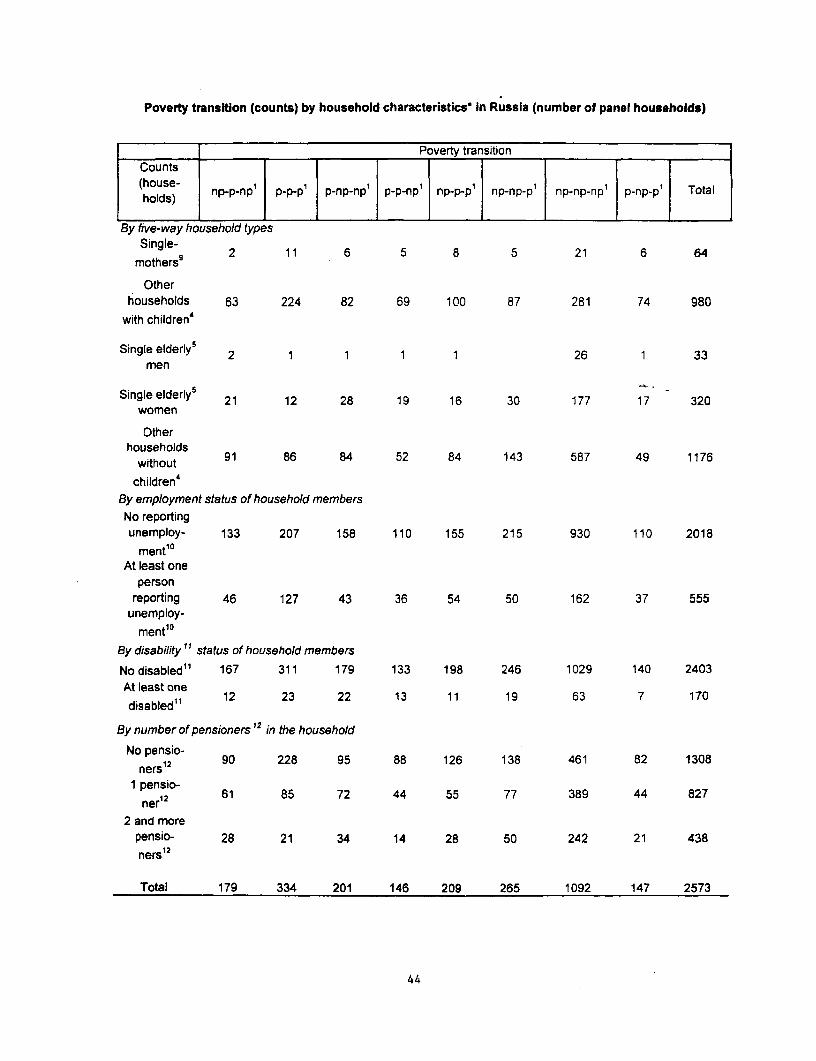
Poverty transition (counts) by household characteristics' in Russia (number of panel households)

Poverty transitionCountsJ

(hols) np-p-np' p-p-p' p-np-np' p-p-np' np-p-p' np-np-pl np-np-npl p-np-p' Total

By five-way household typesSingle- 2 11 6 5 8 5 21 6 64

mothers

Otherhouseholds 63 224 82 69 100 87 281 74 980

with children4

Single elderly5 2 1 1 1 1 26 1 33men

Single elderlyS 21 12 28 19 16 30 177 17 320women

Otherhouseholds

without 91 86 84 52 84 143 587 49 1176children4

By employment status of household membersNo reportingunemploy- 133 207 158 110 155 215 930 110 2018

ment10

At least oneperson

reporting 46 127 43 36 54 50 162 37 555unemploy-

mentl0

By disability' 1 status of household members

No disabled" 167 311 179 133 198 246 1029 140 2403

disabledao 12 23 22 13 11 19 63 7 170

By number of pensioners 12 in the household

No pensio-npersi 12 90 228 95 88 126 138 461 82 1308

I pensio-ner12 61 85 72 44 55 77 389 44 827

2 and morepensio- 28 21 34 14 28 50 242 21 438ners 12

Total 179 334 201 146 209 265 1092 147 2573

44

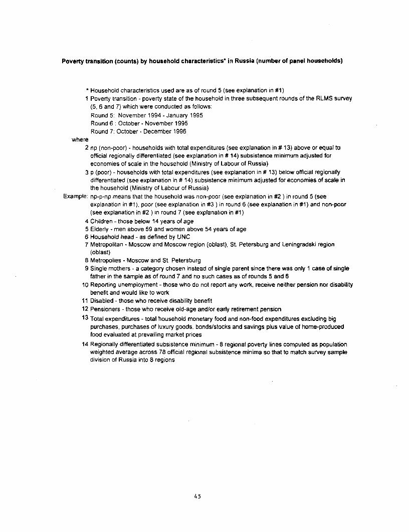
Poverty transition (counts) by household characteristics in Russia (number of panel households)

* Household characteristics used are as of round 5 (see explanation in #1)1 Poverty transition - poverty state of the household in three subsequent rounds of the RLMS survey

(5, 6 and 7) which were conducted as follows:Round 5: November 1994 - January 1995Round 6: October - November 1995Round 7: October - December 1996

where2 np (non-poor) - households with total expenditures (see explanation in # 13) above or equal to

official regionally differentiated (see explanation in # 14) subsistence minimum adjusted foreconomies of scale in the household (Ministry of Labour of Russia)

3 p (poor) - households with total expenditures (see explanation in # 13) below official regionallydifferentiated (see explanation in # 14) subsistence minimum adjusted for economies of scale inthe household (Ministry of Labour of Russia)

Example: np-p-np means that the household was non-poor (see explanation in #2 ) in round 5 (seeexplanation in #1), poor (see explanation in #3 ) in round 6 (see explanation in #1) and non-poor(see explanation in #2 ) in round 7 (see explanation in #1)

4 Children - those below 14 years of age5 Elderly - men above 59 and women above 54 years of age6 Household head - as defined by UNC7 Metropolitan - Moscow and Moscow region (oblast), St. Petersburg and Leningradski region

(oblast)8 Metropolies - Moscow and St. Petersburg9 Single mothers - a category chosen instead of single parent since there was only 1 case of single

father in the sample as of round 7 and no such cases as of rounds 5 and 610 Reporting unemployment - those who do not report any work, receive neither pension nor disability

benefit and would like to work11 Disabled - those who receive disability benefit12 Pensioners - those who receive old-age and/or early retirement pension

13 Total expenditures - total household monetary food and non-food expenditures excluding bigpurchases, purchases of luxury goods, bonds/stocks and savings plus value of home-producedfood evaluated at prevailing market prices

14 Regionally differentiated subsistence minimum - 8 regional poverty lines computed as populationweighted average across 78 official regional subsistence minima so that to match survey sampledivision of Russia into 8 regions

45

Poverty transition (rates) by household characteristics* in Russia (% of panel households)

Poverty transition'Rates (% ofhouseholds) npp-np hpp' p-np-np' p-p-np' np-p-p' np-np-p' np-np-np' p-np-p' Total

By household size

1 6.2 4.4 7.8 6.0 4.4 10.3 55.9 5.1 100.0

2 6.6 5.8 6.2 4.1 7.2 11.5 55.0 3.5 100.03 8.4 12,8 9.7 4.9 11.1 10.8 37.5 4.8 100.04 6.4 21.7 8.1 8.1 8.8 8.1 29.8 9.0 100.0

5 and more 7.0 29.3 7.4 6.3 8.9 10.4 22.6 8.1 100.0

By number of children 4 in the household

No children4 7.5 6.5 7.4 4.7 6.6 11.3 51.7 4.4 100.0

1 child' 7.2 16.5 8.1 6.1 11.3 8.7 34.1 8.1 100.0

2 children4 and more 4.6 32.7 9.0 8.8 8.8 9.0 20.1 7.0 100.0

By number of elderly 5 in the household

No elderly5 6.7 16,6 7.6 6.4 9.8 10.3 36.2 6.4 100.0

1 elderly5 7.5 11.7 8.3 6.0 6.5 9.6 45.0 5.3 100.0

2 and more elderlys 6.6 4.3 7.5 3.0 5.9 11.6 56.6 4.5 100.0

By four-type family composition

No children', 7.5 8.3 7.0 4.5 7.9 13.2 47.2 4.5 100.0

no elderly5

Children4, no elderly5 6.2 22.1 8.1 7.6 11.0 8.4 29.0 7.6 100.0

Elderly5 , no children4 7.4 5.5 7.6 4.8 5.9 10.3 54.1 4.3 100.0

Children4 and elderly5 6.3 23.9 9.7 5.5 8.0 10.1 28.6 8.0 100.0

By gender of household head 6

Female 7.2 8.8 8.5 6.4 7.5 9.1 46.3 6.1 100.0Male 6.9 14.3 7.6 5.4 8.3 10.7 41.2 5.6 100.0

46

Povert transition (rates) by household characteristics' in Russia (% of panel households)

Poverty transition'Rates (% ofhouseholds) np-p-np' p-p-p1 p-np-npl p-p-np' np-p-p' np-np-p' np-np-np' p-np-p' Total

By regions

Metropolitan7 8.9 4.6 8.9 6.3 3.0 7.0 57.6 3.6 100.0

North and North- 8.7 19.7 6.4 6.4 6.4 6.9 41.0 4.6 tO0.0Western

Central and Central 6.5 12.0 8.1 2.9 7.9 8.9 48.6 5 3 100.0Black Earth

Volga and Volgo- 5.9 15.0 6.3 5.7 9.4 11.0 40.7 5.9 100.0Vyatsky basin

North Caucasian 8.2 6.3 11.2 7.2 4.6 10 5 44.7 7.2 100.0

Ural 5.7 17.8 7.0 7.2 8.2 11.9 35.6 6.7 100.0

Western Siberia 8.2 14.5 5.1 4.3 13.7 12.5 34.8 7.0 100.0

Eastern Siberia and 5.4 15 6 10.3 6.3 12.1 12.9 33.0 4.5 100.0Far East

By type of settlement

Metropoliesa 8.8 4.8 9.5 7.0 3.3 6.6 56.8 3.3 100.0

Urban 7.1 13.3 7.2 5.6 8.8 10.1 43.0 5.0 100.0

Rural 6.0 15.3 8.5 5.3 8.5 12.1 36.1 8.0 1-oo0.

By access to land in the household

No 7.2 15.6 9.1 7.6 7.7 7.9 39.9 5.1 100.0Yes 6.9 11.9 7 3 4.9 8.3 11.3 43.5 6.0 100.0

By ownership of car in the household

No 6.8 14.3 8.0 6.3 8.5 10.4 39.3 6.4 100.0Yes 7.4 7.8 7.3 3.4 6.7 10.1 54.2 3.2 100.0

47

Poverty transition (rates) by household characteristics* in Russia (% of panel households)

=_________________ IPoverty transition'

Rates (% ofhouseholds) np-p-np' p-p-p' p-np-np' p-p-npl np-p-p1 np-np-p1 np-np-npl p-np-p' Total

By five-way household typesSingle-mothers9 3.1 17.2 9.4 7.8 12.5 7.8 32.8 9.4 100.0

Other householdswith children4 6.4 22.9 8.4 7.0 10.2 8.9 28.7 76 100.0

Single elderlys men 6.1 3.0 3.0 3.0 3.0 78.8 3.0 100.0

Single elderly5 women 6.6 3.8 8.8 5.9 5.0 9.4 55.3 5.3 100.0

Other householdswithoutchildren4 7.7 7.3 7.1 4.4 7.1 12.2 49.9 4.2 100.0

By employment status of household members

No reporting 6.6 10 3 7.8 5.5 7.7 10.7 46 1 5.5 100.0uJnemployment"

At least one personreporting unemploy- 8.3 22.9 7.7 6.5 9.7 9.0 29.2 6.7 100.0

ment'°By disability " status of household members

No disabled" 6.9 12.9 7.4 5.5 8.2 10.2 428 5.8 100.0At least onedisabled1 7.1 13.5 12.9 7.6 6.5 11.2 37.1 4.1 100.0

By number of pensioners 12 in the household

No pensioners'2 6.9 17.4 7.3 6.7 9.6 10.6 35.2 6.3 100.0

1 pensioner12 7.4 10.3 8.7 5.3 6.7 9.3 47.0 5.3 100.0

2 and more pensio-nd rsio2 6.4 4.8 7.8 3.2 6.4 11.4 55.3 4.8 100.0ners'

Total 7.0 13.0 7.8 5.7 8.1 10.3 42.4 5.7 100.0

48

Poverty transition (rates) by household characteristics* in Russia (% of panel households)

* Household characteristics used are as of round 5 (see explanation in #1)1 Poverty transition - poverty state of the household in three subsequent rounds of the RLMS

survey (5, 6 and 7) which were conducted as follows:Round 5: November 1994 - January 1995Round 6. October - November 1995Round 7: October - December 1996

where2 np (non-poor) - households with total expenditures (see explanation in # 13) above or equal.

to official regionally differentiated (see explanation in # 14) subsistence minimum adjustedfor economies of scale in the household (Ministry of Labour of Russia)

3 p (poor) - households with total expenditures (see explanation in # 13) below officialregionally differentiated (see explanation in # 14) subsistence minimum adjusted foreconomies of scale in the household (Ministry of Labour of Russia)

Example: np-p-np means that the household was non-poor (see explanation in #2 ) in round 5 (seeexplanation in #1), poor (see explanation in #3 ) in round 6 (see explanation in #1) and non-poor (see explanation in #2 ) in round 7 (see explanation in #1)

4 Children - those below 14 years of age5 Elderly - men above 59 and women above 54 years of age6 Household head - as defined by UNC7 Metropolitan - Moscow and Moscow region (oblast), St. Petersburg and Leningradski region

(oblast)8 Metropolies - Moscow and St. Petersburg9 Single mothers - a category chosen instead of single parent since there was only 1 case of

single father in the sample as of round 7 and no such cases as of rounds 5 and 610 Reporting unemployment - those who do not report any work, receive neither pension nor

disability benefit and would like to work1 1 Disabled - those who receive disability benefit12 Pensioners - those who receive old-age and/or early retirement pension

13 Total expenditures - total household monetary food and non-food expenditures excludingbig purchases, purchases of luxury goods, bonds/stocks and savings plus value of home-produced food evaluated at prevailing market prices

14 Regionally differentiated subsistence minimum - 8 regional poverty lines computed aspopulation weighted average across 78 official regional subsistence minima so that to matchsurvey sample division of Russia into 8 regions

49

Poverty transition (composition) by household characteristics* in Russia (% of panel households)

Poverty transition'Composition (% of - I . Ihouseholds)nze p-p-p' p-np-np1 p-p-np1 np-p-p1 np-np-p np-np-np1 p-np-p1 I Total

By household size1 15.1 5.7 16.9 17.8 9.1 17.0 22.3 15.0 16.92 27.4 12.9 22.9 20-5 25.4 32.1 37.2 17.7 28.73 27.4 22.5 28.4 19.9 31.1 23.8 20.1 19.0 22.84 19.6 35.3 21.9 30.1 23.0 16.6 14.8 33.3 21.1

5and more 10.6 23.7 10.0 11.6 11.5 10.6 5.6 15.0 10.5Total 100.0 100.0 100.0 100.0 100.0 100.0 100.0 100.0 100.0

By number of children 4 in the householdNo children4 63.7 29.6 56.2 49.3 48.3 65.3 72.3 45.6 59.4

1 child4 26.3 32.3 26.4 27.4 35.4 21.5 20.5 36.1 25.52 children4 and more 10.1 38.0 17.4 23.3 16.3 13.2 7.1 18.4 15.1

Total 100.0 100.0 100.0 100.0 100.0 100.0 100.0 100.0 100.0By number of elderly5 in the household

No elderly5 50.3 66.5 50.7 58.2 62.7 52.1 44.4 57.8 52.01 elderly5 33.5 27.8 32.8 32.9 24.9 28.7 32.8 28.6 30.9

2 and more elderly5 16.2 5.7 16.4 8.9 12.4 19.2 22.8 13.6 17.1Total 100.0 100.0 100.0 100.0 100.0 100.0 100.0 100.0 100.0

By four-type family compositionNo children', 22.3 13.2 18.4 16.4 20.1 26.4 23.0 16.3 20.7

Children4, no elderlys 27.9 53.3 32.3 41.8 42.6 25.7 21.4 41.5 31.3Elderly5, no children4 41.3 16.5 37.8 32.9 28.2 38.9 49.4 29.3 38.7

Children 4and elderly5 8.4 17.1 11.4 8.9 9.1 9.1 6.2 12.9 9.2Total 100.0 100.0 100.0 100.0 100.0 100.0 100.0 100.0 100.0

By gender of household head6Female 25.1 16.5 26.4 27.4 22.5 21.5 26.5 25.9 24.3Male 74.9 83.5 73.6 72.6 77.5 78.5 73.5 74.1 75.7Total 100.0 100.0 100.0 100.0 100.0 100.0 100.0 100.0 100.0

Poverty transition (composition) by household characteristics* in Russia (% of panel households)

Poverty transition'

Composition (% of np-p-np' p-p-p' I p-np-np' p-p-np' np-p-p' np-np-p' np-np-np' p-np-p' TotalBy regions

Metropolitan7 15.1 4.2 13.4 13.0 4.3 7.9 15.9 7.5 11.7

North and North- 8.4 10.2 5.5 7.5 5.3 4.5 6.5 5.4 6.7Western

CentralandCentral 15.1 15.0 16.9 8.2 15.8 14.0 18.6 15.0 16.2Black Earth

Volga and Volgo- 16.8 22.8 15.9 19.9 23.0 21.1 19.0 20.4 19.7Vyatsky basin

North Caucasian 14.0 5.7 16.9 15.1 6.7 12 1 12 5 15.0 11.8

Ural 12.3 20.7 13.4 19.2 15 3 17.4 12.6 17.7 15.1

Western Siberia 11.7 11.1 6.5 7.5 16.7 12.1 8.2 12.2 9.9Eastern Siberia and 6.7 10.5 11.4 9.6 12 9 10.9 6.8 6.8 8.7

U, Far EastTotal 100.0 100.0 100.0 100.0 100.0 100.0 100.0 100 0 100.0

By type of settlement

Metropolies8 13.4 3.9 12.9 13.0 4.3 6.8 14.2 6.1 10.6Urban 61.5 61.7 55.2 59.6 65.1 58.9 61.0 53.1 60 2

Rural 25.1 34.4 31.8 27.4 30.6 34.3 24.8 40.8 29.1

Total 100.0 100.0 100.0 100.0 100.0 100.0 100 0 100.0 100.0

By access to land in the household

No 30.2 35.0 33.8 39.0 27.8 22.3 27.5 25.9 29.2Yes 69.8 65.0 66.2 61.0 72.2 77.7 72.5 74.1 70.8Total 100.0 100.0 100.0 100.0 100.0 100.0 100.0 100.0 100.0

By ownership of car in the householdNo 77.7 87.4 80.6 87.7 82.8 79.6 73.4 88.4 79.1

Yes 22.3 12.6 19.4 12.3 17.2 20.4 26.6 11.6 20.9Total 100.0 100.0 100.0 100.0 100.0 100.0 100.0 100.0 100.0

Poverty transition (composition) by household characteristics* in Russia (% of panel households)

Poverty transition'

Composition (Y of np-p-np'p p p-np-npl p-p-np' | np-p-p' np-np-p1 np-np-np' p p-np-p' Total

By five-way household types

Single-mothers9 1.1 3.3 3.0 3.4 3.8 1.9 1.9 4.1 2.5Other households with

children4 35.2 67.1 40.8 47.3 47.8 32.8 25.7 50.3 38.1

Single elderly5 men 1.1 0.3 0.5 0.7 0.5 2.4 0.7 1.3

Single elderly5 women 11.7 3.6 13.9 13.0 7.7 11.3 16.2 11.6 12.4

Other households

without children4 50.8 25.7 41.8 35.6 40.2 54.0 53.8 33.3 45.7Total 100.0 100.0 100.0 100.0 100.0 100.0 100.0 100.0 100.0

By employment status

No reporting10 74.3 62.0 78.6 75.3 74.2 81.1 85.2 74.8 78.4, ~~~~unemploymentrAt least one personreporting unemploy- 25.7 38.0 21.4 24.7 25.8 18.9 14.8 25.2 21.6

mentl°Total 100.0 100.0 100.0 100.0 100.0 100.0 100.0 100.0 100.0

By disability " status of household members

No disabled'1 93.3 93.1 89.1 91.1 94.7 92.8 94.2 95.2 93.4

At least one disabled" 6.7 6.9 10.9 8.9 5.3 7.2 5.8 4.8 6.6

Total 100.0 100.0 100.0 100.0 100.0 100.0 100.0 100.0 100.0By number of pensioners ' 2 in the household

No pensioners12 50.3 68.3 47.3 60.3 60.3 52.1 42.2 55.8 50.8

1 pensioner12 34.1 25.4 35.8 30.1 26.3 29.1 35.6 29.9 32.12 and more pensio- 15.6 6.3 16.9 9.6 13.4 18.9 22.2 14.3 17.0

nersl0Total 100.0 100.0 100.0 100.0 100.0 100.0 100.0 100.0 100.0

Poverty transition (composition) by household characteristics* In Russia (% of panel households)

* Household characterstics used are as of round 5 (see explanation in #11)1 Poverty transition - poverty state of the household in three subsequent rounds of the RLMS survey (5,

6 and 7) which were conducted as follows:Round 5: November 1994 - January 1995Round 6: October - November 1995Round 7: October - December 1996

where2 np (non-poor) - households with total expenditures (see explanation in # 13) above or equal to official

regionally differentiated (see explanation in # 14) subsistence minimum adjusted for economies ofscale in the household (Ministry of Labour of Russia)

3 p (poor) - households with total expenditures (see explanation in # 13) below official regionallydifferenbated (see explanation in # 14) subsistence minimum adjusted for economies of scale in thehousehold (Ministry of Labour of Russia)

Example: np-p-np means that the household was non-poor (see explanation in #2 ) in round 5 (see explanationin #1), poor (see explanation in #3 ) in round 6 (see explanation in #1) and non-poor (see explanationin #2 ) in round 7 (see explanation in #1)

4 Children - those below 14 years of ageLi 5 Elderly - men above 59 and women above 54 years of age

6 Household head - as defined by UNC7 Metropolitan - Moscow and Moscow region (oblast), St. Petersburg and Leningradski region (oblast)8 Metropolies - Moscow and St. Petersburg9 Single mothers - a category chosen instead of single parent since there was only 1 case of single

father in the sample as of round 7 and no such cases as of rounds 5 and 610 Reporting unemployment - those who do not report any work, receive neither pension nor disability

benefit and would like to work11 Disabled - those who receive disability benefit12 Pensioners - those who receive old-age and/or early retirement pension13 Total expenditures - total household monetary food and non-food expenditures excluding big

purchases, purchases of luxury goods, bonds/stocks and savings plus value of home-produced foodevaluated at prevailing market prices

14 Regionally differentiated subsistence minimum - 8 regional poverty lines computed as populationweighted average across 78 official regional subsistence minima so that to match survey sampledivision of Russia into 8 regions

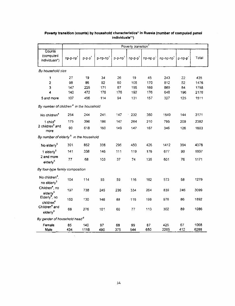
Poverty transition (counts) by household characteristics* in Russia (number of computed panelindividuals"*)

Poverty transition'Counts

(ncvduatse np-p-np p-p-p p-np-np p-p-np1 np-p-p' np-np-p' np-np-np' p-np-p1 Total

By household size

1 27 19 34 26 19 45 243 22 4352 98 86 92 60 106 170 812 52 14763 147 225 171 87 195 189 660 84 17584 140 472 176 176 192 176 648 196 2176

Sandmore 107 456 114 94 131 157 327 125 1511

By number of children 4in the household

hlo children4 254 244 241 147 232 360 1549 144 3171

1 child4 175 396 186 147 264 210 795 209 23822 children4 and 90 618 160 149 147 167 346 126 1803

more

By number of elderly 5 in the household

No elderly5 301 852 338 295 450 426 1412 304 4378

i elderly5 141 338 146 111 119 176 677 99 1807

2 and morey5 77 68 103 37 74 135 601 76 1171

elderly

By four-type family composition

No children4, 104 114 93 59 116 162 573 58 1279

no elderly5

Children;, no 197 738 245 236 334 264 839 246 3099

elderVyElderly . no 150 130 148 88 116 198 976 86 1892

children4

Children4and 68 276 101 60 77 113 302 89 1086

elderly5

By gender of household head S

Female 85 140 97 68 99 87 425 67 1068Male 434 1118 490 375 544 650 2265 412 6288

54

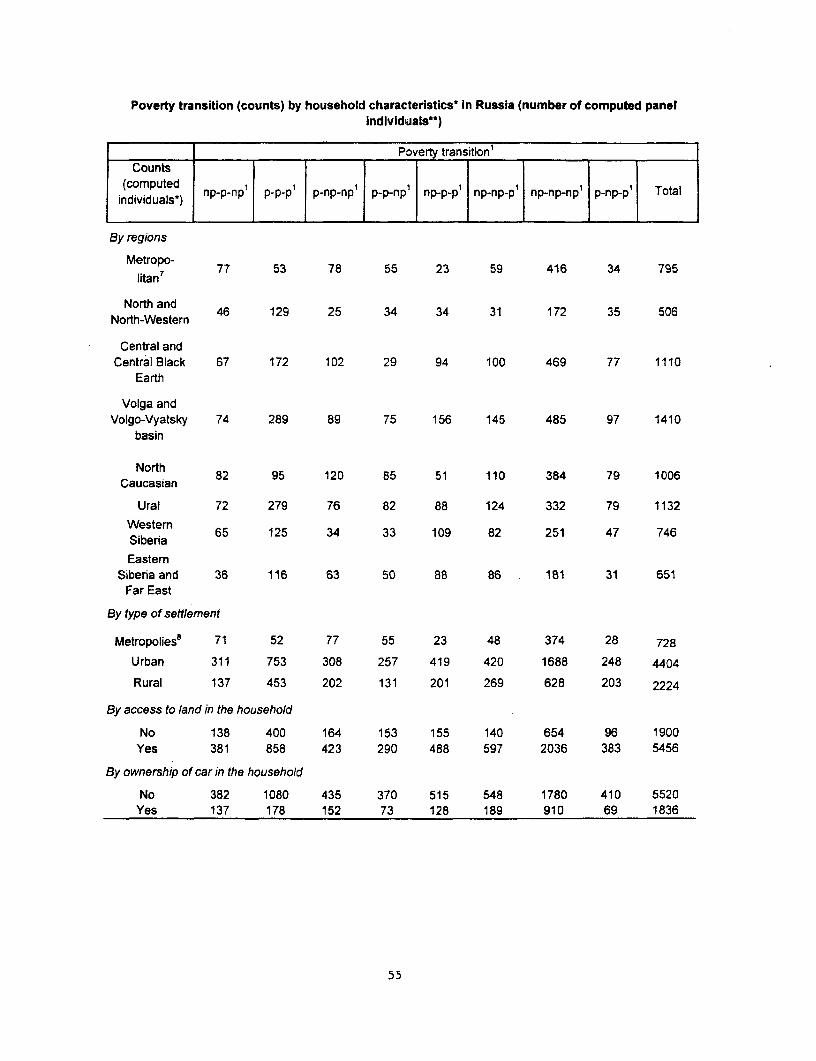
Poverty transition (counts) by household characteristics* in Russia (number of computed panelindividuals')

Poverty transition'Counts

(computed np1 p 1np

individuals) np-p-np p-p-p p-np-npl p-p-np' np-p-p' np-np-p' np-np-npl p-np-p' Total

By regions

litan7 77 53 78 55 23 59 416 34 795

North and 46 129 25 34 34 31 172 35 506North-Western

Central andCentral Black 67 172 102 29 94 100 469 77 1110

Earth

Volga andVolgo-Vyatsky 74 289 89 75 156 145 485 97 1410

basin

North 82 95 120 85 51 110 384 79 1006Caucasian

Ural 72 279 76 82 88 124 332 79 1132Westerm 65 125 34 33 109 82 251 47 746Siberia

EasternSiberia and 36 116 63 50 88 86 181 31 651

Far East

By type of settlement

Metropolies8 71 52 77 55 23 48 374 28 728

Urban 311 753 308 257 419 420 1688 248 4404

Rural 137 453 202 131 201 269 628 203 2224

By access to land in the household

No 138 400 164 153 155 140 654 96 1900Yes 381 858 423 290 488 597 2036 383 5456

By ownership of car in the household

No 382 1080 435 370 515 548 1780 410 5520Yes 137 178 152 73 128 189 910 69 1836

55

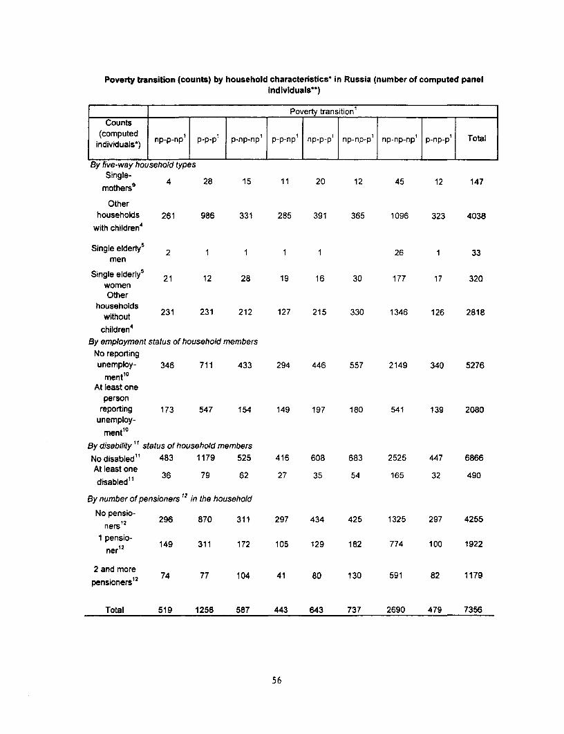
Poverty transition (counts) by household characteristics* in Russia (number of computed panelIndividuals**)

Poverty transition'Counts

(cdputdua np-p-np' p-p-p' p-np-npl p-p-npl np-p-pl np-np-pl np-np-np' p-np-p1 Total

By five-way household types

Single- 4 28 15 11 20 12 45 12 147mothers9

Otherhouseholds 261 986 331 285 391 365 1096 323 4038

with children4

Single elderly5 2 1 1 1 1 26 1 33men

Single elderly5 21 12 28 19 16 30 177 17 320womenOther

households 231 231 212 127 215 330 1346 126 2818

children4

By employment status of household membersNo reportingunemploy- 346 711 433 294 446 557 2149 340 5276

mentl 0

At least oneperson

reporting 173 547 154 149 197 180 541 139 2080unemploy-

mentl0

By disability " status of household membersNo disabled"1 483 1179 525 416 608 683 2525 447 6866

At least one 36 79 62 27 35 54 165 32 490

By number of pensioners ' 2 in the household

nensio2 296 870 311 297 434 425 1325 297 4255ners1

1 pensio-nern12 149 311 172 105 129 182 774 100 1922

2 and morepensioners' 2 74 77 104 41 80 130 591 82 1179

Total 519 1258 587 443 643 737 2690 479 7356

56

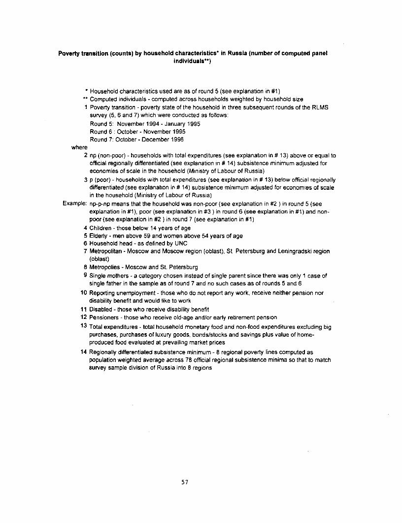
Poverty transition (counts) by household characteristics' in Russia (number of computed panelindividuals")

Household characteristics used are as of round 5 (see explanation in #1)Computed individuals - computed across households weighted by household size

1 Poverty transition - poverty state of the household in three subsequent rounds of the RLMSsurvey (5, 6 and 7) which were conducted as follows:Round 5: November 1994 - January 1995Round 6: October - November 1995Round 7: October- December 1996

where2 np (non-poor) - households with total expenditures (see explanation in # 13) above or equal to

official regionally differentiated (see explanation in # 14) subsistence minimum adjusted foreconomies of scale in the household (Ministry of Labour of Russia)

3 p (poor) - households with total expenditures (see explanation in # 13) below official regionallydifferentiated (see explanation in # 14) subsistence minimum adjusted for economies of scalein the household (Ministry of Labour of Russia)

Example: np-p-np means that the household was non-poor (see explanation in #2 ) in round 5 (seeexplanation in #1), poor (see explanation in #3 ) in round 6 (see explanation in #1) and non-poor (see explanation in #2 ) in round 7 (see explanation in #1)

4 Children - those below 14 years of age5 Elderly - men above 59 and women above 54 years of age6 Household head - as defined by UNC7 Metropolitan - Moscow and Moscow region (oblast), St. Petersburg and Leningradski region

(oblast). Metropolies - Moscow and St. Petersburg9 Single mothers - a category chosen instead of single parent since there was only 1 case of

single father in the sample as of round 7 and no such cases as of rounds 5 and 610 Reporting unemployment - those who do not report any work, receive neither pension nor

disability benefit and would like to work11 Disabled - those who receive disability benefit12 Pensioners - those who receive old-age and/or early retirement pension13 Total expenditures - total household monetary food and non-food expenditures excluding big

purchases, purchases of luxury goods, bonds/stocks and savings plus value of home-produced food evaluated at prevailing market prices

14 Regionally differentiated subsistence minimum - 8 regional poverty lines computed aspopulation weighted average across 78 official regional subsistence minima so that to matchsurvey sample division of Russia into 8 regions

57

Poverty transition (rates) by household characteristics* in Russia (% of computed panel individuals')

Poverty transition'Rates (% of computed

individuals*) np-p-np' p-p-pl p-np-npl p-p-np' np-p-p' np-np-p' np-np-np' p-np-p1 Total

By household size

1 6.2 4.4 7.8 6.0 4.4 10.3 55.9 5.1 10.02 6.6 5.8 6.2 4.1 7.2 11.5 55.0 3.5 100.03 8.4 12.8 9.7 4.9 11.1 10.8 37.5 4.8 100.04 6.4 21.7 8.1 8.1 8.8 8.1 29.8 9.0 100.0

5 and more 7.1 30.2 7.5 6.2 8 7 10.4 21.6 8.3 1000

By number of children 4 in the household

No children4 8.0 7.7 7.6 4.6 7.3 11.4 48.8 4.5 100.0

1 child4 7.3 16.6 7.8 6.2 11.1 8.8 33.4 8.8 100.0

2 children4 and more 5.0 34.3 8.9 8.3 8.2 9.3 19.2 7.0 100.0

By number of elderly 5 in the household

No elderly5 6.9 19.5 7.7 6,7 10.3 9.7 32.3 6.9 100.0

1 elderly5 7.8 18.7 8.1 6.1 6.6 9.7 37.5 5.5 1000

2 and more elderly5 6.6 5.8 8.8 3.2 6.3 11.5 51.3 6.5 100.0

By four-type family composition

No children4 , 8.1 8.9 7.3 4.6 9.1 12.7 44.8 4.5 100.0

no elderly5

Children4 , no elderly5 6.4 23.8 7.9 7.6 10.8 8.5 27.1 7.9 100.0

Elderly5, no children4 7.9 6.9 7.8 4.7 61 10.5 51.6 4.5 100.0

Children4 and elderly5 6.3 25.4 9.3 5.5 71 10.4 27.8 8.2 100.0

By gender of household head6

Female 8.0 13.1 9.1 6.4 9.3 8.1 39.8 6.3 100.0Male 6.9 17.8 7.8 6.0 8.7 10.3 36.0 6.6 100.0

58

Poverty transition (rates) by household characteristics* in Russia (% of computed panel individuals')

Poverty transition'Rates (% of computed

individuals*) np-p-np' p-p-p' p-np-np' p-p-np' np-P-P' np-np-p' np-np-np' p-np-p' Total

By regions

Metropolitan7 9.7 6.7 9.8 6.9 2 9 7 4 52 3 4.3 100.0

North and North- 9.1 25.5 4.9 6 7 6 7 6.1 34.0 6.9 100.0Western

Central and Central 6.0 15.5 9.2 2.6 8 5 9.0 42.3 6.9 100.0Black Earth

Volga and Volgo- 5.2 20.5 6.3 5 3 11.1 10.3 34.4 6.9 100.0Vyatsky basin

North Caucasian 8.2 9 4 11 9 8 4 5.1 10 9 38.2 7.9 100 0

Ural 6.4 24.6 6 7 7.2 7.8 11 0 29.3 7.0 100.0

Western Siberia 8.7 16.8 46 4.4 14 6 11.0 33.6 6.3 100.0

Eastern Siberia and 5.5 17.8 9.7 7.7 13.5 13.2 27.8 4.8 100 0Far East

By type of settlement

Metropolies8 9.8 7.1 10.6 7.6 3.2 6 6 51.4 3 8 100.0

Urban 7.1 17.1 7.0 5.8 9.5 9.5 383 5.6 100.0

Rural 6.2 20.4 9. 1 5.9 9.0 12.1 28.2 9.1 100.0

By access to land in the household

No 7.3 21.1 8.6 8.1 8.2 7.4 34.4 5.1 100.0Yes 7.0 15.7 7.8 5 3 8 9 10.9 37.3 7.0 100.0

By ownership of car in the household

No 6.9 19.6 7.9 6.7 9.3 9.9 32.2 7.4 100.0Yes 7.5 9.7 8.3 4.0 7 0 10.3 49.6 3.8 100.0

59

Poverty transition (rates) by household characteristics* in Russia (% of computed panel individuals')

Poverty transition'Rates (% of computed

individuals*) np-p-np' p-p-p' p-np-np' p-p-np' np-p-p' np-np-p' np-np-np' p-np-p' Total

By five-way household typesSingle-mothers9 2.7 19.0 10.2 7.5 13.6 8.2 30.6 8.2 100.0

Other householdswithchildren4 6.5 24.4 8.2 7.1 9.7 9.0 27.1 8.0 100.0

Single elderly5 men 6.1 3.0 3.0 3.0 3.0 78.8 3.0 100.0

Single elderlys women 6.6 3.8 8.8 5.9 5.0 9.4 55.3 5.3 100.0

Other householdswithoutchildren4 8.2 8.2 7.5 4.5 7.6 11.7 47.8 4.5 100.0

By employment status of household members

uNo reporting 6.6 13.5 8.2 5.6 8.5 10.6 40.7 6.4 100.0unemployment'°

At least one personreporting unemploy- 8.3 26.3 7.4 7.2 9.5 8.7 26.0 6.7 100.0

ment'o

By disability " status of household members

No disabled" 7.0 17.2 7.6 6.1 8.9 9.9 36.8 6.5 100.0At least onedisabled" 7.3 16.1 12.7 5.5 7.1 11.0 33.7 6.5 100.0

By number of pensioners 12 in the household

No pensioners"2 7.0 20.4 7.3 7.0 10,2 10.0 31.1 7.0 100.0

1 pensioner"2 7.8 16.2 8.9 5.5 6.7 9.5 40.3 5.2 100.02 and more pensio-

tners12 6.3 6.5 8.8 3.5 6.8 11.0 50.1 7.0 100.0ners"

Total 7.1 17.1 8.0 6.0 8.7 10.0 36.6 6.5 100.0

60

Poverty transition (rates) by household characteristics^ in Russia (% of computed panel individuals*)

Household characteristics used are as of round 5 (see explanation in #1)Computed individuals - computed across households weighted by household size

1 Poverty transition - poverty state of the household in three subsequent rounds of the RLMSsurvey (5, 6 and 7) which were conducted as follows:Round 5 November 1994 - January 1995Round 6: October - November 1995Round 7: October - December 1996

where2 np (non-poor) - households with total expenditures (see explanation in # 13) above or equal

to official regionally differentiated (see explanation in # 14) subsistence minimum adjustedfor economies of scale in the household (Ministry of Labour of Russia)

3 p (poor) - households with total expenditures (see explanation in # 13) below ofFicialregionally differentiated (see explanation in # 14) subsistence minimum adjusted foreconomies of scale in the household (Ministry of Labour of Russia)

Example np-p-np means that the household was non-poor (see explanation in #2 ) in round 5 (seeexplanation in #1), poor (see explanation in #3 ) in round 6 (see explanation in #1) and non-poor (see explanation in #2 ) in round 7 (see explanation in #1)

4 Children - those below 14 years of age5 Elderly - men above 59 and women above 54 years of age6 Household head - as defined by UNC7 Metropolitan - Moscow and Moscow region (oblast), St. Petersburg and Leningradski

region (oblast)8 Metropolies - Moscow and St. Petersburg9 Single mothers - a category chosen instead of single parent since there was only I case of

single father in the sample as of round 7 and no such cases as of rounds 5 and 610 Reporting unemployment - those who do not report any work, receive neither pension nor

disability benefit and would like to work1 1 Disabled - those who receive disability benefit12 Pensioners - those who receive old-age and/or early retirement pension13 Total expenditures - total household monetary food and non-food expenditures excluding

big purchases, purchases of luxury goods, bonds/stocks and savings plus value of home-produced food evaluated at prevailing market prices

14 Regionally differentiated subsistence minimum - 8 regional poverty lines computed aspopulation weighted average across 78 official regional subsistence minima so that tomatch survey sample division of Russia into 8 regions

61

Poverty transition (composition) by household characteristics* in Russia (% of computed panel individuals*)

Poverty transition'Compustediondivduls of IComposition (% of dus np-p-np | ppp1 I p-np-np1 p-p-np' np-p-p' np-np-p' np-np-np1 p-np-p1 I Total

By household size

1 5.2 1.5 5.8 5.9 3.0 6.1 9.0 4.6 5.92 18.9 6.8 15.7 13.5 16.5 23.1 30.2 10.9 20.13 28.3 17.9 29.1 19.6 30.3 25.6 24.5 17.5 23.94 27.0 37.5 30.0 39.7 29.9 23,9 24.1 40.9 29.6

5 and more 20.6 36.2 19.4 21.2 20.4 21.3 12.2 26.1 20.5Total 100.0 100.0 100.0 100.0 100.0 100.0 100.0 100.0 100.0

By number of children' in the householdNo children4 48.9 19.4 41.1 33.2 36.1 48.8 57.6 30.1 43.1

1 child4 33.7 31.5 31.7 33.2 41.1 28.5 29.6 43.6 32.42 children4 and more 17.3 49.1 27.3 33.6 22.9 22.7 12.9 26.3 24.5

Total 100.0 100.0 100.0 100.0 100.0 100.0 100.0 100.0 100.0By number of elderly5 in the household

No elderly5 58.0 67.7 57.6 66.6 70.0 57.8 52.5 63.5 59.51 elderly5 27.2 26.9 24.9 25.1 18.5 23.9 25.2 20.7 24.6

2 and more elderly' 14.8 5.4 17.5 8.4 11.5 18.3 22.3 15.9 15.9Total 100.0 100.0 100.0 100.0 100.0 100.0 100.0 100.0 100.0

By four-type family composition

No children', no 20.0 9.1 15.8 13.3 18.0 22.0 21.3 12.1 17.4Children4, no elderly5 38.0 58.7 41.7 53.3 51.9 35.8 31.2 51.4 42.1Elderly5, no children4 28.9 10.3 25.2 19.9 18.0 26.9 36.3 18.0 25.7Children4andelderly5 13.1 21.9 17.2 13.5 12.0 15.3 11.2 18.6 14.8

Total 100.0 100.0 100.0 100.0 100.0 100.0 100.0 100.0 100.0By gender of household head6

Female 16.4 11.1 16.5 15.3 15.4 11.8 15.8 14.0 14.5Male 83.6 88.9 83.5 84.7 84.6 88.2 84.2 86.0 85.5Total 100.0 100.0 100.0 100.0 100.0 100.0 100.0 100.0 100.0

Poverty transition (composition) by household characteristics* in Russia (% of computed panel individuals'*)

Poverty transition'

Compositon (% of i da) np-p-np P-p 1 I p-np-np' p-p-npl np-p-p' np-np-p' np-np-np' p-np-p' Totalcomputed individuals) By regions

Metropolitan7 14.8 4.2 13.3 12.4 3.6 8.0 15.5 7.1 10.8

North and North- 8.9 10.3 4.3 7.7 5.3 4.2 6.4 7.3 6.9Westem

Central and Central 12.9 13.7 17.4 6.5 14.6 13.6 17.4 16.1 15.1Black Earth

Volga and Volgo- 14.3 23.0 15.2 16.9 24.3 19.7 18.0 20.3 19.2Vyatsky basin

North Caucasian 15.8 7.6 20.4 19.2 7.9 14.9 14.3 16.5 13.7

Ural 13.9 22.2 12.9 18.5 13.7 16.8 12.3 16.5 15.4Westem Siberia 12.5 9.9 5.8 7.4 17 0 11.1 9.3 9.8 10.1

EasternSiberiaandFar 6.9 9.2 10.7 11.3 137 11.7 6.7 6.5 8.8oa East

Total 100.0 100.0 100.0 100.0 100.0 100.0 100.0 100.0 100.0By type of settlement

Metropolies8 13.7 4.1 13.1 12.4 3.6 6.5 13.9 5.8 9.9Urban 59.9 59.9 52.5 58.0 65.2 57.0 62.8 51.8 59.9

Rural 26.4 36.0 34 4 29.6 31.3 36.5 23.3 42.4 30.2

Total 100.0 100.0 100.0 100.0 100.0 100.0 100.0 100.0 100.0By access to land in the household

No 26.6 31.8 27.9 34.5 24.1 19.0 24 3 20.0 25.8Yes 73.4 68.2 72.1 65.5 75.9 81.0 75.7 80.0 74 2

Total 100.0 100.0 100.0 100.0 100.0 100.0 100.0 100.0 100.0By ownership of car in the household

No 73.6 85.9 74.1 83.5 80.1 74.4 66.2 85.6 75.0Yes 26.4 14.1 25.9 16.5 19.9 25.6 33.8 14.4 25.0Total 100.0 100.0 100.0 100.0 100.0 100.0 100.0 100.0 100.0

Poverty transition (composition) by household characteristics* in Russia (% of computed panel individuals")

Poverty transition'

computed individuals) np-p-np p-p-p I p-np-np' p-p-np' np-p-p| np-np-p np-np-np' p-np-p' TotalBy five-way household types

Single-mothers9 0.8 2.2 2.6 2.5 3.1 1.6 1.7 2.5 2.0

Other households withchildren4 50.3 78.4 56.4 64.3 60.8 49.5 40.7 67 4 54.9

Single elderly5 men 0.4 0.1 0.2 0.2 0.2 1.0 0.2 0.4

Single elderly5 women 4.0 1.0 4.8 4.3 2.5 4.1 6.6 3.5 4.4Other householdswithoutchildren 445 18.4 36.1 28.7 33.4 44.8 50.0 26.3 38.3

Total 100.0 100.0 100.0 100.0 100.0 100.0 100.0 100.0 100 0By employment status

No reportinguNorempoyment' 66 7 56.5 73.8 66.4 69.4 75.6 79.9 71.0 71.7

unemployment'(0*. At least one person

reporting unemploy- 33.3 43.5 26.2 33.6 30.6 24.4 20.1 29.0 28.3

ment'"Total 100.0 100.0 100.0 100.0 100.0 100.0 100.0 100.0 100.0

By disability " status of household members

No disabled" 93.1 93.7 89.4 93.9 94.6 92.7 93.9 93.3 93.3

Atleastonedisabled" 6.9 6.3 10.6 6.1 5.4 7,3 6.1 67 6.7

Total 100.0 100.0 100.0 100.0 100.0 100.0 100.0 100.0 100.0

By number of pensioners ' 2 in the household

No pensioners'2 57.0 69.2 53.0 67.0 67.5 57.7 49.3 62.0 57.8

1 pensioner'2 28.7 24.7 29.3 23.7 20.1 24.7 28.8 20.9 26.1

2 and more pensio-2 and er 1eo- 14.3 6.1 17.7 9.3 12.4 17.6 22.0 17.1 16.0ners'lTotal 100.0 100.0 100.0 100.0 100.0 100.0 100.0 100.0 100.0

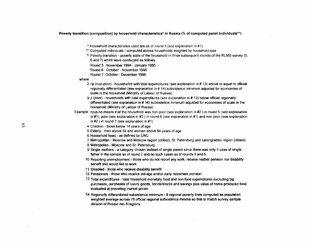
Poverty transition (composition) by household characteristics* in Russia (% of computed panel individuals**)

* Household characteristics used are as of round 5 (see explanation in #1)

Computed individuals - computed across households weighted by household size

1 Poverty transition - poverty state of the household in three subsequent rounds of the RLMS survey (5,

6 and 7) which were conducted as follows:

Round 5: November 1994 - January 1995Round 6: October - November 1995Round 7: October - December 1996

where2 np (non-poor) - households with total expenditures (see explanation in # 13) above or equal to official

regionally differentiated (see explanation in # 14) subsistence minimum adjusted for economies of

scale in the household (Ministry of Labour of Russia)

3 p (poor) - households with total expenditures (see explanation in # 13) below official regionally

differentiated (see explanation in # 14) subsistence minimum adjusted for economies of scale in the

household (Ministry of Labour of Russia)Example: np-p-np means that the household was non-poor (see explanation in #2 ) in round 5 (see explanation

in #1), poor (see explanation in #3 ) in round 6 (see explanation in #1) and non-poor (see explanation

in #2 ) in round 7 (see explanation in #1)4 Children - those below 14 years of age5 Elderly - men above 59 and women above 54 years of age

6 Household head - as defined by UNC7 Metropolitan - Moscow and Moscow region (oblast), St. Petersburg and Leningradski region (oblast)

8 Metropolies - Moscow and St. Petersburg9 Single mothers - a category chosen instead of single parent since there was only 1 case of single

father in the sample as of round 7 and no such cases as of rounds 5 and 6

10 Reporting unemployment - those who do not report any work, receive neither pension nor disability

benefit and would like to work11 Disabled - those who receive disability benefit12 Pensioners - those who receive old-age and/or early retirement pension

13 Total expenditures - total household monetary food and non-food expenditures excluding big

purchases, purchases of luxury goods, bonds/stocks and savings plus value of home-produced food

evaluated at prevailing market prices

14 Regionally differentiated subsistence minimum - 8 regional poverty lines computed as population

weighted average across 78 official regional subsistence minima so that to match survey sample

division of Russia into 8 regions

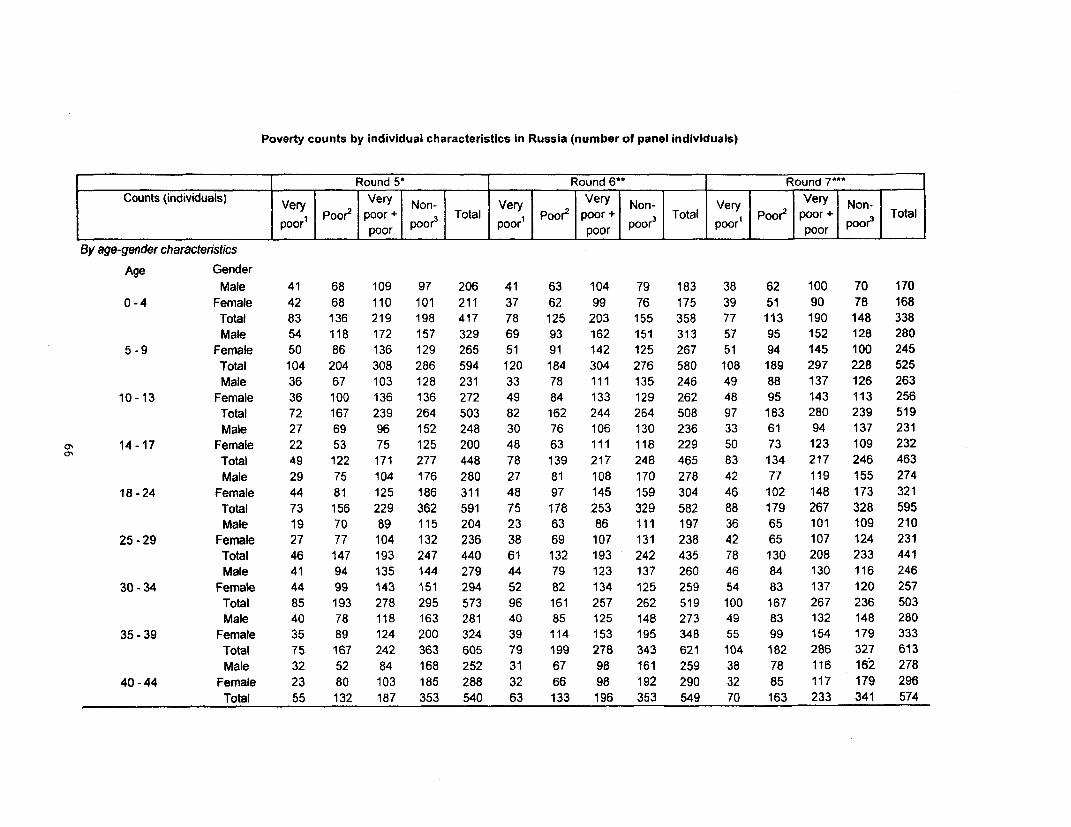
Poverty counts by individual characteristics in Russia (number of panel individuals)

Round 5^ Round 6** Round 7***Counts (individuals) Very Very Non- Very Very Non- Very Very Non-

poor' Poor2 poor+ poor3 Total poor' Poor' poor poor3 Total poor, Poor2 poor+ poo Total

By age-gender characteristics

Age GenderMale 41 68 109 97 206 41 63 104 79 183 38 62 100 70 170

0-4 Female 42 68 110 101 211 37 62 99 76 175 39 51 90 78 168Total 83 136 219 198 417 78 125 203 155 358 77 113 190 148 338Male 54 118 172 157 329 69 93 162 151 313 57 95 152 128 280

5 - 9 Female 50 86 136 129 265 51 91 142 125 267 51 94 145 100 245Total 104 204 308 286 594 120 184 304 276 580 108 189 297 228 525Male 36 67 103 128 231 33 78 111 135 246 49 88 137 126 263

10-13 Female 36 100 136 136 272 49 84 133 129 262 48 95 143 113 256Total 72 167 239 264 503 82 162 244 264 508 97 183 280 239 519Male 27 69 96 152 248 30 76 106 130 236 33 61 94 137 231

114-17 Female 22 53 75 125 200 48 63 111 118 229 50 73 123 109 232Total 49 122 171 277 448 78 139 217 248 465 83 134 217 246 463Male 29 75 104 176 280 27 81 108 170 278 42 77 119 155 274

18-24 Female 44 81 125 186 311 48 97 145 159 304 46 102 148 173 321Total 73 156 229 362 591 75 178 253 329 582 88 179 267 328 595Male 19 70 89 115 204 23 63 86 111 197 36 65 101 109 210

25 - 29 Female 27 77 104 132 236 38 69 107 131 238 42 65 107 124 231Total 46 147 193 247 440 61 132 193 242 435 78 130 208 233 441Male 41 94 135 144 279 44 79 123 137 260 46 84 130 116 246

30 - 34 Female 44 99 143 151 294 52 82 134 125 259 54 83 137 120 257Total 85 193 278 295 573 96 161 257 262 519 100 167 267 236 503Male 40 78 118 163 281 40 85 125 148 273 49 83 132 148 280

35 - 39 Female 35 89 124 200 324 39 114 153 195 348 55 99 154 179 333Total 75 167 242 363 605 79 199 278 343 621 104 182 286 327 613Male 32 52 84 168 252 31 67 98 161 259 38 78 116 162 278

40 -44 Female 23 80 103 185 288 32 66 98 192 290 32 85 117 179 296Total 55 132 187 353 540 63 133 196 353 549 70 163 233 341 574

Poverty counts by individual characteristics in Russia (number of panel individuals)

Round 5* Round 6** Round 7***Counts (individuals) Very Very Non- Very Very Non- Very Very Non-

poor' Poor' poor + poOr Totail poor: Poor' poor poor3 Total poorl Poor2 poor + poor3 Total

By age-gender characteristics (continued)

Age GenderMale 11 42 53 130 183 18 51 69 142 211 22 71 93 124 217

45 - 49 Female 17 59 76 159 235 26 67 93 173 266 37 67 104 170 274Total 28 101 129 289 418 44 118 162 315 477 59 138 197 294 491Male 19 37 56 105 161 14 36 50 92 142 13 32 45 68 113

50-54 Female 11 29 40 118 158 14 30 44 87 131 14 45 59 86 145Total 30 66 96 223 319 28 66 94 179 273 27 77 104 154 258Male 11 43 54 167 221 18 43 61 155 216 24 58 82 145 227

55 - 59 Female 14 64 78 249 327 21 60 81 235 316 26 59 85 213 298Total 25 107 132 416 548 39 103 142 390 532 50 117 167 358 525Male 10 22 32 153 185 7 21 28 131 159 15 28 43 112 155

60 - 64 Female 16 38 54 179 233 18 42 60 180 240 27' 44 71 165 236Total 26 60 86 332 418 25 63 88 311 399 42 72 114 277 391Male 8 22 30 126 156 9 30 39 141 180 19 33 52 137 189

65-69 Female 21 43 64 200 264 21 52 73 208 281 30 72 102 183 285Total 29 65 94 326 420 30 82 112 349 461 49 105 154 320 474Male 8 19 27 99 126 6 22 28 108 136 7 18 25 120 145

70 and older Female 47 90 137 259 396 42 86 128 299 427 57 92 149 309 458Total 55 109 164 358 522 48 108 156 407 563 64 110 174 429 603

By employment-gender status

Unemployment4 GenderMale 328 776 1104 1924 3028 359 791 1150 1841 2991 399 835 1234 1678 2912

Not reporting Female 398 965 1363 2318 3681 470 963 1433 2263 3696 526 1014 1540 2135 3675Total 726 1741 2467 4242 6709 829 1754 2583 4104 6687 925 1849 2774 3813 6587Male 58 100 158 156 314 51 97 148 150 298 89 98 187 179 366

Reporting Female 51 91 142 191 333 66 102 168 169 337 82 112 194 166 360Total 109 191 300 347 647 117 199 316 319 635 171 210 381 345 726

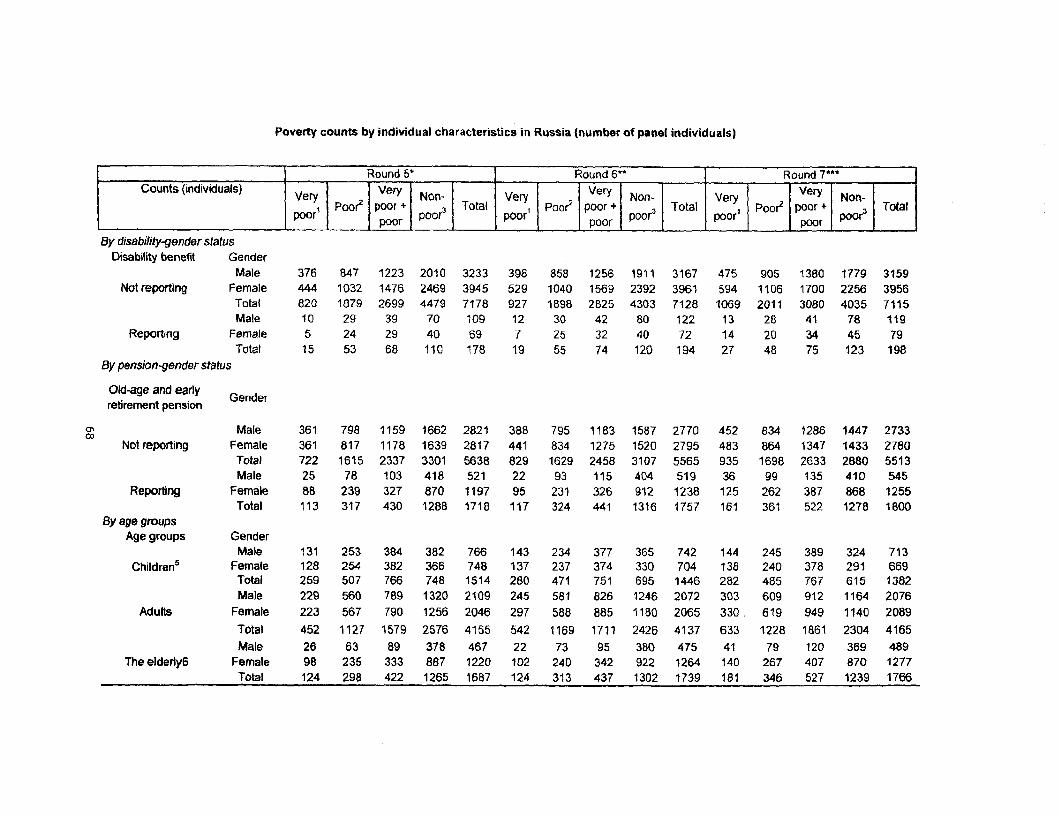
Poverty counts by individual characteristics in Russia (number of panel individuals)

Round 5* Round 6* Round 7***Counts (individuals) Very Very Non- Very Very Non- VrVery Non-

poor' Poor p pooroooa Poor' poor + poor 3 Total poor' Poor2 poor p Total

By disability-ender statusDisability benefit Gender

Male 376 847 1223 2010 3233 398 858 1256 1911 3167 475 905 1380 1779 3159Not reporting Female 444 1032 1476 2469 3945 529 1040 1569 2392 3961 594 1106 1700 2256 3956

Total 820 1879 2699 4479 7178 927 1898 2825 4303 7128 1069 2011 3080 4035 7115Male 10 29 39 70 109 12 30 42 80 122 13 28 41 78 119

Reporting Female 5 24 29 40 69 7 25 32 40 72 14 20 34 45 79Total 15 53 68 110 178 19 55 74 120 194 27 48 75 123 198

By pension-gender status

Old-age and early Genderretirement pension

Male 361 798 1159 1662 2821 388 795 1183 1587 2770 452 834 1286 1447 2733Notreporting Female 361 817 1178 1639 2817 441 834 1275 1520 2795 483 864 1347 1433 2780

Total 722 1615 2337 3301 5638 829 1629 2458 3107 5565 935 1698 2633 2880 5513Male 25 78 103 418 521 22 93 115 404 519 36 99 135 410 545

Reporting Female B8 239 327 870 1197 95 231 326 912 1238 125 262 387 868 1255Total 113 317 430 1288 1718 117 324 441 1316 1757 161 361 522 1278 1800

By age groupsAge groups Gender

Male 131 253 384 382 766 143 234 377 365 742 144 245 389 324 713Children5 Female 128 254 382 366 748 137 237 374 330 704 138 240 378 291 669

Total 259 507 766 748 1514 280 471 751 695 1446 282 485 767 615 1382Male 229 560 789 1320 2109 245 581 826 1246 2072 303 609 912 1164 2076

Adults Female 223 567 790 1256 2046 297 588 885 1180 2065 330 619 949 1140 2089Total 452 1127 1579 2576 4155 542 1169 1711 2426 4137 633 1228 1861 2304 4165Male 26 63 89 378 467 22 73 95 380 475 41 79 120 369 489

The eldeuly6 Female 98 235 333 887 1220 102 240 342 922 1264 140 267 407 870 1277Total 124 298 422 1265 1687 124 313 437 1302 1739 181 346 527 1239 1766

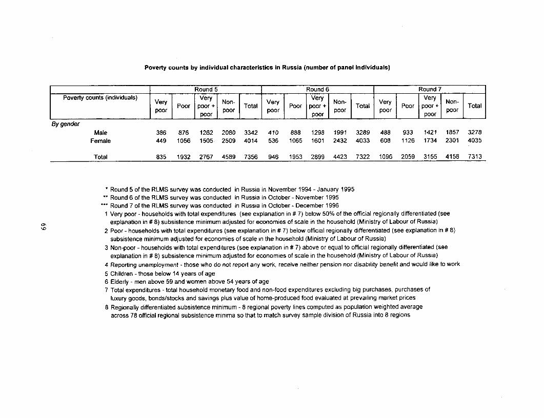
Poverty counts by individual characteristics in Russia (number of panel individuals)

Round 5 Round 6 Round 7Poverty counts (individuals) Very Very Non- Very Very Non- Very Very Non-

poor Poor poor + poor Total poor Poor poor + poor Total poor Poor poor + poor Totalpoo porpor oo porpoor poor poor

By genderMale 386 876 1262 2080 3342 410 888 1298 1991 3289 488 933 1421 1857 3278

Female 449 1056 1505 2509 4014 536 1065 1601 2432 4033 608 1126 1734 2301 4035

Total 835 1932 2767 4589 7356 946 1953 2899 4423 7322 1096 2059 3155 4158 7313

* Round 5 of the RLMS survey was conducted in Russia in November 1994 - January 1995Round 6 of the RLMS survey was conducted in Russia in October - November 1995Round 7 of the RLMS survey was conducted in Russia in October - December 1996

1 Very poor - households with total expenditures (see explanation in # 7) below 50% of the official regionally differentiated (seea'> explanation in # 8) subsistence minimum adjusted for economies of scale in the household (Ministry of Labour of Russia)

2 Poor - households with total expenditures (see explanation in # 7) below official regionally differentiated (see explanation in # 8)subsistence minimum adjusted for economies of scale in the household (Ministry of Labour of Russia)

3 Non-poor - households with total expenditures (see explanation in # 7) above or equal to official regionally differentiated (seeexplanation in # 8) subsistence minimum adjusted for economies of scale in the household (Ministry of Labour of Russia)

4 Reporting unemployment - those who do not report any work, receive neither pension nor disability benefit and would like to work5 Children - those below 14 years of age6 Elderly - men above 59 and women above 54 years of age7 Total expenditures - total household monetary food and non-food expenditures excluding big purchases, purchases of

luxury goods, bonds/stocks and savings plus value of home-produced food evaluated at prevailing market prices8 Regionally differentiated subsistence minimum - 8 regional poverty lines computed as population weighted average

across 78 official regional subsistence minima so that to match survey sample division of Russia into 8 regions

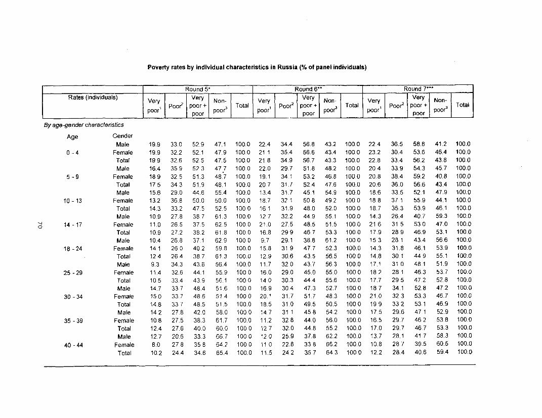
Poverty rates by individual characteristics in Russia (% of panel individuals)

Round 5- Round 6** Round 7***Rates (individuals) Very Very Non- Very Very Non- Very Very Non-

p Poor2 poor + poor3 Total poor' poor2 poor + pOoe Total poor' Poor2 poor + poor] Totalpo porpoporpo 3poor poor poor

By age-gender characteristics

Age GenderMale 19.9 33.0 52.9 47.1 100.0 22.4 34.4 56.8 43.2 100.0 22.4 36.5 58.8 41.2 100.0

0 - 4 Female 19.9 32.2 52.1 47.9 100.0 21.1 35.4 56.6 43.4 100.0 23.2 30.4 53.6 46.4 100.0Total 19.9 32.6 52.5 47.5 100.0 21.8 34.9 56.7 43.3 100.0 22.8 33.4 56.2 43.8 100.0Male 16.4 35.9 52.3 47.7 100.0 22.0 29.7 51.8 48.2 100.0 20.4 33.9 54.3 45.7 100.0

5 - 9 Female 18.9 32.5 51.3 48.7 100.0 19.1 34.1 53.2 46.8 100.0 20.8 38.4 59.2 40.8 100.0Total 17.5 34.3 51.9 48.1 100.0 20.7 31,7 52.4 47.6 100.0 20.6 36.0 56.6 43.4 100.0Male 15.6 29.0 44.6 55.4 100.0 13.4 31.7 45.1 54.9 100.0 18,6 33.5 52 1 47.9 100.0

10 - 13 Female 13.2 36.8 50.0 50.0 100.0 18.7 32 1 50.8 49.2 100 0 18.8 37 1 55.9 44.1 100.0Total 14.3 33.2 47.5 52.5 100.0 16.1 31.9 48.0 52.0 100.0 18.7 35.3 53.9 46.1 100.0Male 10.9 27.8 38.7 61.3 100.0 12.7 32.2 44.9 55.1 100.0 14.3 26.4 40.7 59.3 100.0

C 14 -17 Female 11.0 26.5 37.5 62.5 100.0 21.0 27.5 48.5 51.5 100.0 21.6 31 5 530 47.0 100.0Total 10.9 27.2 38.2 61.8 100.0 16.8 29 9 46,7 53.3 100.0 17.9 28.9 46.9 53.1 100.0Male 10.4 26.8 37.1 62.9 100.0 9.7 29.1 38.8 61.2 100,0 15.3 28 1 43.4 56.6 100.0

18-24 Female 14.1 26.0 40.2 59.8 100.0 15.8 31.9 47.7 52.3 100.0 14.3 31.8 46.1 53.9 100.0Total 124 26.4 38,7 61.3 100.0 12.9 30.6 43.5 56.5 1000 14.8 30,1 44.9 55.1 100.0Male 9.3 34.3 43.6 56.4 100.0 11.7 32.0 43.7 56.3 100.0 17.1 31.0 481 51.9 100.0

25-29 Female 11.4 32.6 44.1 55.9 100.0 16.0 29.0 45.0 55.0 100.0 18.2 28.1 46.3 53.7 100.0Total 10,5 334 43 9 56.1 100.0 14.0 30.3 44.4 55.6 100.0 17 7 29 5 47 2 52.8 100.0Male 14.7 33.7 48.4 51.6 100.0 16 9 30.4 47.3 52.7 100.0 18.7 34.1 52.8 47.2 100.0

30-34 Female 15.0 33.7 48.6 51.4 100.0 20.1 31.7 51.7 48.3 100.0 21.0 323 53.3 46.7 100.0Total 14.8 33.7 48.5 51.5 1000 18.5 31.0 49.5 50.5 100.0 19.9 33.2 53.1 46.9 100.0Male 14 2 27 8 42.0 58.0 100.0 14.7 31.1 45 8 54.2 100 0 17 5 29.6 47.1 52.9 100.0

35 - 39 Female 10.8 27.5 38.3 61.7 100.0 11.2 32.8 44.0 56.0 100.0 16.5 29 7 462 53.8 100.0Total 12.4 27.6 40.0 60.0 100.0 12.7 32 0 44 8 55.2 100.0 17.0 29.7 46.7 53.3 100.0Male 127 20.6 33.3 66.7 100.0 12.0 25.9 37.8 62.2 100.0 13.7 28 1 41,7 58.3 100.0

40 - 44 Female 8.0 27.8 35.8 64.2 100.0 11.0 22.8 33,8 66.2 100.0 10.8 28.7 39.5 60.5 100.0Total 10.2 24.4 34.6 65.4 100.0 11.5 24.2 35 7 64.3 100 0 12.2 28.4 40.6 59.4 100.0

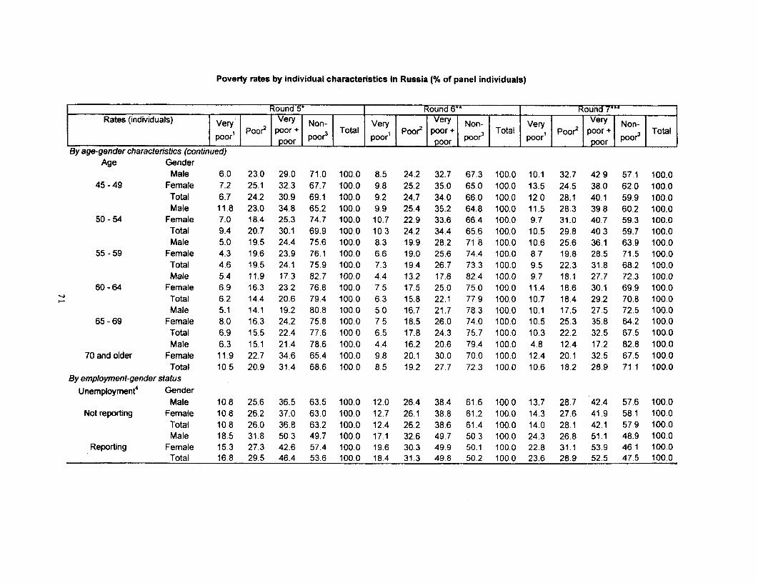
Poverty rates by individual characteristics in Russia (% of panel individuals)

Round 5* Round 6** Round 7***Rates (individuals) Ve Very Non- Very Very Non- Very Very Non-

Pr' Poor' poor3+ Total poor poor o 3 Total Poor2 poor3+ Totalp .oo poor poorp poor poor poor' or poor

By age-gender characteristics (continued)Age Gender

Male 6.0 23.0 29.0 71.0 100.0 8.5 24.2 32.7 67.3 100.0 10.1 32.7 42.9 57.1 100.045-49 Female 7.2 25.1 32.3 67.7 100.0 9.8 25.2 35.0 65.0 100.0 13.5 24.5 38.0 62.0 100.0

Total 6.7 24.2 30.9 69.1 100.0 9.2 24.7 34.0 66.0 100.0 12.0 28.1 40.1 59.9 100.0Male 11.8 23.0 34.8 65.2 100.0 9.9 25.4 35.2 64.8 100.0 11.5 28.3 39.8 60.2 100.0

50 - 54 Female 7.0 18.4 25.3 74.7 100.0 10.7 22.9 33.6 66.4 100.0 9.7 31.0 40.7 59.3 100.0Total 9.4 20.7 30.1 69.9 100.0 10.3 24.2 34.4 65.6 100.0 10.5 29.8 40 3 59.7 100.0Male 5.0 19.5 24.4 75.6 100.0 8.3 19.9 28.2 71.8 100.0 10.6 25.6 36.1 63.9 100.0

55-59 Female 4.3 19.6 23.9 76.1 100.0 6.6 19.0 25.6 74.4 100.0 8.7 19.8 28.5 71.5 100.0Total 4.6 19.5 24.1 75.9 100.0 7.3 19.4 26.7 73.3 100.0 9.5 22.3 31.8 68.2 100.0Male 5.4 11.9 17.3 82.7 100.0 4.4 13.2 17.6 82.4 100.0 9.7 18.1 27.7 72.3 100.0

60-64 Female 6.9 16.3 23.2 76.8 100.0 7.5 17.5 25.0 75.0 100.0 11.4 18.6 30.1 69.9 100.02 Total 6.2 14.4 20.6 79.4 100.0 6.3 15.8 22.1 77.9 100.0 10.7 18.4 29.2 70.8 100.0

Male 5.1 14.1 19.2 80.8 100.0 5.0 16.7 21.7 78.3 100.0 10.1 17.5 27.5 72.5 100.065-69 Female 8.0 16.3 24.2 75.8 100.0 7.5 18.5 26.0 74.0 100.0 10.5 25.3 35.8 64.2 100.0

Total 6.9 15.5 22.4 77.6 100.0 6.5 17.8 24.3 75.7 100.0 10.3 22.2 32.5 67.5 100.0Male 6.3 15.1 21.4 78.6 100.0 4.4 16.2 20.6 79.4 100.0 4.8 12.4 17.2 82.8 100.0

70 and older Female 11.9 22.7 34.6 65.4 100.0 9.8 20.1 30.0 70.0 100.0 12.4 20.1 32.5 67.5 100.0Total 10.5 20.9 31.4 68.6 100 0 8.5 19.2 27.7 72.3 100.0 10.6 18.2 28.9 71.1 100.0

By employment-gender statusUnemployment4 Gender

Male 10.8 25.6 36.5 63.5 100.0 12.0 26.4 38.4 61.6 100.0 13.7 28.7 42.4 57.6 100.0Not reporting Female 10.8 26.2 37.0 63.0 100.0 12.7 26.1 38.8 61.2 100.0 14.3 27.6 419 58.1 100.0

Total 10.8 26.0 36.8 63.2 100.0 12.4 26.2 38.6 61.4 100.0 14.0 28.1 42.1 57.9 100.0Male 18.5 31.8 50.3 49.7 100.0 17.1 32.6 49.7 50.3 100.0 24.3 26.8 51.1 48.9 100.0

Reporting Female 15.3 27.3 42.6 57.4 100.0 19.6 30.3 49.9 50.1 100.0 22.8 31.1 53.9 46.1 100.0Total 16.8 29.5 46.4 53.6 100.0 18.4 31.3 49.8 50.2 100.0 23.6 28.9 52.5 47.5 100.0

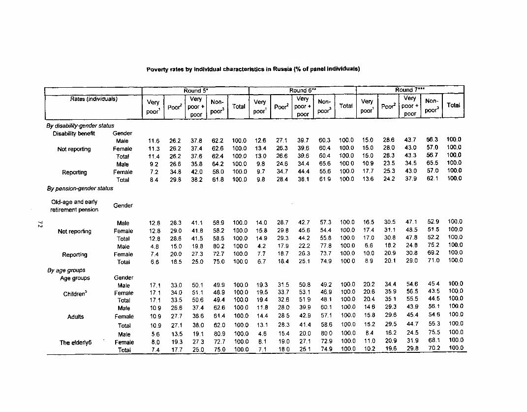
Poverty rates by individual characteristics in Russia (% of panel individuals)

Round 5* Round 6" Round 7*^^Rates (individuals) Very Very Non- Very Very Non- Very Very Non-

r poor2 poor + Total Poor2 poor + 3 Total Poore poor + 3 Totalpoor' poo poor poorp poor poor POOr

By disability-gender statusDisability benefit Gender

Male 11.6 26.2 37.8 62.2 100.0 12.6 27.1 39.7 60.3 100.0 15.0 28.6 43.7 56.3 100.0Notreporting Female 11.3 26.2 37.4 62.6 100.0 13.4 26.3 39.6 60.4 100.0 15.0 28.0 43.0 57.0 100.0

Total 11.4 26.2 37.6 62.4 100.0 13.0 26.6 39.6 60.4 100.0 15.0 28.3 43.3 56.7 100.0Male 9.2 26.6 35.8 64.2 100.0 9.8 24.6 34.4 65.6 100.0 10.9 23.5 34.5 65.5 100.0

Reporting Female 7.2 34.8 42.0 58.0 100.0 9.7 34.7 44.4 55.6 100.0 17.7 25.3 43.0 57.0 100.0Total 8.4 29.B 38.2 61.8 100.0 9.8 28.4 38.1 61.9 100.0 13.6 24.2 37.9 62.1 100.0

By pension-gender status

Old-age and early Genderretirement pension

_j Male 12.8 28.3 41.1 58.9 100.0 14.0 28.7 42.7 57.3 100.0 16.5 30.5 47.1 52.9 100.0Not reporling Female 12.8 29.0 41.8 58.2 100.0 15.8 29.8 45.6 54.4 100.0 17.4 31.1 48.5 51.5 100.0

Total 12.8 28.6 41.5 58.5 100.0 14.9 29.3 44.2 55.8 100.0 17.0 30.8 47.8 52.2 100.0Male 4.8 15.0 19.8 80.2 100.0 4.2 17.9 22.2 77.8 100.0 6.6 18.2 24.8 75.2 100.0

Reporting Female 7.4 20.0 27.3 72.7 100.0 7.7 18.7 26.3 73.7 100.0 10.0 20.9 30.8 69.2 100.0Total 6.6 18.5 25.0 75.0 100.0 6.7 18.4 25.1 74.9 100.0 8.9 20.1 29.0 71.0 100.0

By age groupsAge groups Gender

Male 17.1 33.0 50.1 49.9 100.0 19.3 31.5 50.8 49.2 100.0 20.2 34.4 54.6 45 4 100.0Children' Female 17.1 34.0 51.1 48.9 100.0 19.5 33.7 53.1 46.9 100.0 20.6 35.9 56.5 43.5 100.0

Total 17.1 33.5 50.6 49.4 100.0 19.4 32.6 51.9 48.1 100.0 20.4 35.1 55.5 44.5 100.0Male 10.9 26.6 37.4 62.6 100.0 11.8 28.0 39.9 60.1 100.0 14.6 29.3 43.9 56.1 100.0

Adults Female 10.9 27.7 38.6 61.4 100.0 14.4 28.5 42.9 57.1 100.0 15.8 29.6 45.4 54.6 100.0Total 10.9 27.1 38.0 62.0 100.0 13.1 28.3 41.4 58.6 100.0 15.2 29.5 44.7 55.3 100.0Male 5.6 13.5 19.1 80.9 100.0 4.6 15.4 20.0 80.0 100.0 8.4 16.2 24.5 75.5 100.0

Theeldery6 Female 8.0 19.3 27.3 72.7 100.0 8.1 19.0 27.1 72.9 100.0 11.0 20.9 31.9 68.1 100.0Total 7,4 17.7 25.0 75.0 100.0 7.1 18.0 25.1 74.9 100.0 10.2 19.6 29.8 70.2 100.0

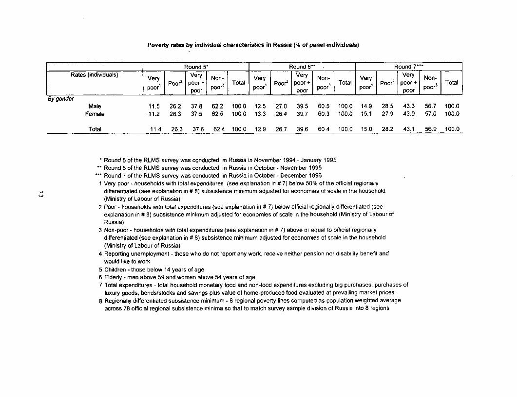
Poverty rates by individual characteristics in Russia (% of panel individuals)

Round 5' Round 6** Round 7***Rates (individuals) Very Very Non- Very Very Non- Very Very Non-

iPoore poor + T otal 1Poor` poor i- Total 1Poor2 poor + 3 Totalpoorr poor2 poor poor' poorp poor3 poor' poo poor

By genderMale 11.5 26.2 37.8 62.2 100.0 12.5 27.0 39.5 60.5 100.0 14.9 28.5 43.3 56.7 100.0

Female 11.2 26.3 37.5 62.5 100.0 13.3 26.4 39.7 60.3 100.0 15.1 27.9 43.0 57.0 100.0

Total 11.4 26.3 37.6 62.4 100.0 12.9 26.7 39.6 60.4 100.0 15.0 28.2 43.1 56.9 100.0

* Round 5 of the RLMS survey was conducted in Russia in November 1994 - January 1995Round 6 of the RLMS survey was conducted in Russia in October - November 1995

*^* Round 7 of the RLMS survey was conducted in Russia in October - December 19961 Very poor - households with total expenditures (see explanation in # 7) below 50% of the official regionally

differentiated (see explanation in # 8) subsistence minimum adjusted for economies of scale in the household(Ministry of Labour of Russia)

2 Poor - households with total expenditures (see explanation in # 7) below official regionally differentiated (seeexplanation in # 8) subsistence minimum adjusted for economies of scale in the household (Ministry of Labour ofRussia)

3 Non-poor - households with total expenditures (see explanation in # 7) above or equal to official regionallydifferentiated (see explanation in # 8) subsistence minimum adjusted for economies of scale in the household(Ministry of Labour of Russia)

4 Reporting unemployment - those who do not report any work, receive neither pension nor disability benefit andwould like to work

5 Children - those below 14 years of age6 Elderly - men above 59 and women above 54 years of age7 Total expenditures - total household monetary food and non-food expenditures excluding big purchases, purchases of

luxury goods, bonds/stocks and savings plus value of home-produced food evaluated at prevailing market pricesB Regionally differentiated subsistence minimum - 8 regional poverty lines computed as population weighted average

across 78 official regional subsistence minima so that to match survey sample division of Russia into 8 regions

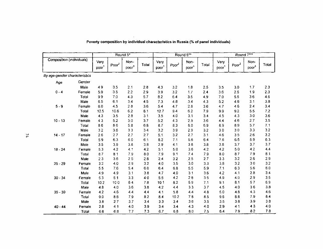
Poverty composition by individual characteristics in Russia (% of panel individuals)

Round 5* Round 6- Round 7***Composition (individuals) Very Non- Very Non- Very Non-

poor1 Poor' poor 3 Total p oor' 2po poor 3 Total poor' Poor2 poor' Total

By age-gender characteristics

Age GenderMale 4.9 3.5 2.1 2.8 4.3 3.2 1.8 2.5 3.5 3.0 1.7 2.3

0 - 4 Female 5.0 3.5 2.2 2.9 3.9 3.2 1.7 2.4 3.6 2.5 1.9 2.3Total 9.9 7.0 4.3 5.7 8.2 6.4 3.5 4.9 7.0 5.5 3.6 4.6Male 6.5 6.1 3.4 4.5 7.3 4.8 3.4 4.3 5.2 4.6 3.1 3.8

5 - 9 Female 6.0 4.5 2.8 3.6 5.4 4.7 2.8 3.6 4.7 4.6 2.4 3.4Total 12.5 10.6 6.2 8.1 12.7 9.4 6.2 7.9 9.9 9,2 5.5 7.2Male 4.3 3.5 2.8 3.1 3.5 4.0 3.1 3.4 4.5 4.3 3.0 3.6

10 - 13 Female 4.3 5.2 3.0 3.7 5.2 4.3 2.9 3.6 4.4 4.6 2.7 3.5Total 8.6 8.6 5.8 6.8 8.7 8.3 6.0 6.9 8.9 8 9 5.7 7.1Male 3.2 3.6 3.3 3.4 3.2 3.9 2.9 3.2 3.0 3.0 3.3 3.2

14 - 17 Female 2.6 2.7 2.7 2.7 5.1 3.2 2.7 3.1 4.6 3 5 2.6 3.2Total 5.9 6.3 6.0 6.1 8.2 7.1 5.6 6.4 7.6 6.5 5.9 6.3Male 3.5 3.9 3.8 3.8 2.9 4.1 3.8 3.8 3.8 3.7 3.7 3.7

18 -24 Female 5.3 4.2 4.1 4.2 5.1 5.0 3.6 4.2 4.2 5.0 4.2 4.4Total 8.7 8.1 7.9 8.0 7.9 9.1 7.4 7.9 8.0 8.7 7.9 8.1Male 2.3 3.6 2.5 2.8 2.4 3.2 2.5 2.7 3.3 3.2 2.6 2.9

25 - 29 Female 3.2 4.0 2.9 3.2 4.0 3.5 3.0 3.3 3.8 3.2 3 0 3.2Total 5.5 7.6 5.4 6.0 6.4 6.8 5.5 5.9 7.1 6.3 5.6 6.0Male 4.9 4.9 3.1 3.8 4.7 4.0 3.1 3.6 4.2 4.1 2 8 3.4

30- 34 Female 5.3 5.1 3.3 4.0 5.5 4.2 2.8 3.5 4.9 4.0 2.9 3.5Total 10.2 10.0 6.4 7.8 10.1 8.2 5.9 7.1 9.1 8. 1 5 7 6.9Male 4.8 4.0 3.6 3.8 4.2 4.4 3.3 3.7 4.5 4.0 3.6 3.8

35 - 39 Female 4.2 4.6 4.4 4.4 4.1 5.8 4.4 4.8 5.0 4.8 4 3 4.6Total 9.0 8.6 7.9 8.2 8.4 10.2 7.8 8.5 9.5 8.8 7.9 8.4Male 3.8 2.7 3.7 3.4 3.3 3.4 3.6 3.5 3.5 3.8 3.9 3.8

40-44 Female 2.8 4.1 4.0 3.9 3.4 3.4 4.3 4.0 2.9 4.1 4 3 4.0Total 6.6 6.8 7.7 7.3 6.7 6.8 8.0 7.5 6.4 7.9 8.2 7.8

Poverty composition by individual characteristics in Russia (% of panel individuals)

Round 5* Round 6" Round 7***Composition (individuals) Very POO| Non- Total ery Non- Total Very pOOr2 Non- Total

Poor2II FoOr3 Toa poor' Pooi-2 poor~ Toa poor' Poo2 TtaBy age-gender characteristics (continued)

Age GenderMale 1.3 2.2 2.8 2.5 1.9 2.6 3.2 2.9 2.0 3.4 3.0 3.0

45-49 Female 2.0 3.1 35 3.2 2.7 3.4 3.9 3.6 3.4 3.3 4.1 3.7Total 3.4 5.2 6.3 5.7 4 7 6.0 7.1 6.5 5.4 6.7 7.1 6.7Male 2.3 1.9 2.3 2.2 1.5 1.8 2.1 1.9 1.2 1.6 1.6 1 5

50 - 54 Female 1.3 1.5 2.6 2.1 1.5 1.5 2.0 1.8 1.3 2.2 2.1 2.0Total 3.6 3.4 4.9 4,3 3.0 3.4 4.0 3.7 2.5 3.7 3.7 3 5Male 1.3 2.2 36 3.0 1.9 2.2 3.5 30 2.2 2.8 3.5 3.1

55-59 Female 1.7 3.3 5.4 4.4 2.2 3.1 5.3 4.3 2.4 2.9 5.1 41Total 3.0 5.5 9.1 7.4 4.1 5.3 8.8 7.3 4.6 5.7 8.6 7.2Male 1.2 1.1 3.3 2.5 0.7 1.1 3.0 2.2 1.4 1.4 2.7 2.1

60-64 Female 1.9 2.0 3.9 3.2 1.9 2.2 4.1 3 3 2.5 2.1 4.0 3.2Total 3.1 3.1 7.2 5.7 2.6 3.2 7.0 5.4 3 8 3.5 6.7 5.3Male 1.0 1.1 2.7 2.1 1.0 1.5 3.2 2.5 1.7 1.6 3.3 2.6

65 - 69 Female 2.5 2.2 44 3.6 2.2 2.7 4.7 3.8 2.7 3.5 4.4 3.9Total 3.5 3.4 7.1 5.7 3.2 4.2 7.9 6.3 4.5 5.1 7.7 6 5Male 1.0 1.0 22 1.7 0.6 1.1 2.4 1.9 0.6 0.9 2.9 2.0

70 and older Female 5.6 4.7 5.6 5.4 4.4 4.4 6.8 5.8 5.2 4.5 7.4 6.3Total 6.6 5.6 78 7.1 5.1 5.5 9.2 7.7 5.8 5.3 10.3 8.2

Total 100.0 100.0 100.0 100.0 100.0 100 0 100.0 100.0 100.0 100.0 1000 100.0By employment-gender status

Unemployment4 GenderMale 39.3 402 41.9 41.2 37.9 40.5 41.6 40.8 36.4 40.6 40.4 39.8

Not reporting Female 47.7 49.9 50.5 50.0 49.7 49.3 51.2 50.5 48.0 49.2 51.3 50.3Total 86.9 90.1 92.4 91.2 87.6 89.8 92.8 91.3 84.4 89.8 917 90.1Male 6.9 5.2 3.4 4.3 5.4 5.0 3.4 4.1 8.1 4.8 4.3 5.0

Reporting Female 6.1 4.7 4.2 4.5 7.0 5.2 3.8 4.6 7.5 5.4 4.0 4.9Total 13.1 9.9 7.6 8.8 12.4 10.2 7.2 8.7 15.6 10.2 8.3 9.9

Total 100.0 100.0 100.0 100.0 100.0 100.0 100.0 100.0 100.0 100.0 100.0 100.0

Poverty composition by individual characteristics in Ru3sia (% of panel individuals)

Round 5* Round 6* Round 7...Composition (individuals) Vr I pooer Non- VerN Very Poo oPor Poroor or opoor oo 3Po or 3 Ttl poor'I' I or Tol

By disability-ender statusDisability benefit Gender

Male 45.0 43.8 43.8 44.0 42.1 43.9 43.2 43.3 43.3 44.0 42.8 43.2Not reporting Female 53.2 53.4 53.8 53.6 55.9 53.3 54.1 54.1 54.2 53.7 54.3 54.1Total 98.2 97t3 97.6 97.6 98.0 97.2 97.3 97-4 97.5 97.7 97.0 97.3Male 1.2 1.5 1.5 1.5 1.3 1.5 1.8 1.7 1.2 1.4 1.9 1.6Reporting Female 0.6 1.2 0.9 0.9 0.7 1.3 0.9 1.0 1.3 1.0 1.1 1.1Total 1.8 2.7 2.4 2.4 2.0 2.8 2.7 2.6 2.5 2.3 3.0 2.7Total 100.0 100.0 100.0 100.0 100.0 100.0 100.0 100.0 100.0 100.0 100.0 100.0By pension-ender status

Old-age and earlyretirement pensionGnd

Male 43.2 41.3 36.2 38.3 41.0 40.7 35,9 37.8 41.2 40.5 34.8 37.4a' Not reporting Female 43.2 42.3 35.7 38.3 46.6 42.7 34.4 38.2 44.1 42.0 34.5 38.0Total 86.5 83.6 71.9 76.6 87.6 83.4 70.2 76.0 85.3 82.5 69.3 75.4Male 3.0 4.0 9.1 7.1 2.3 4.8 9.1 7.1 3.3 4.8 9.9 7.5Reporting Female 10.5 12.4 19.0 16.3 10.0 11.8 20.6 16.9 11.4 12.7 20.9 17.2Total 13.5 16.4 28.1 23.4 12.4 16.6 29.8 24.0 14.7 17.5 30.7 24.6Total 100.0 100.0 100.0 100.0 100.0 100.0 100.0 100.0 100.0 100.0 100.0 100.0By age groupsAge groups Gender

Male 15.7 13.1 8.3 10.4 15.1 12.0 8.3 10.1 13.1 11.9 7.8 97Children5 Female 15.3 13.1 8.0 10.2 14-5 12.1 7.5 9.6 12.6 11.7 7 0 9.1Total 31.0 26.2 16.3 20.6 29.6 24.1 15.7 19.7 25.7 23.6 14.8 18.9Male 27.4 29.0 28.8 28,7 25.9 29.7 28.2 28.3 27.6 29.6 28.0 28.4Adults Female 26.7 29.3 27.4 27.8 31.4 30.1 26.7 26.2 30.1 30.1 27.4 28.6Total 54.1 58.3 56.1 56.5 57.3 59.9 54.8 56.5 578 59.6 55.4 57.0Male 3.1 3.3 8.2 6.3 2.3 3.7 8.6 6 5 3.7 3.8 8.9 6.7Theelderly6 Female 11.7 12.2 19.3 16.6 10.8 12.3 20.8 17.3 12.8 13.0 20.9 17.5Total 14.9 15.4 27.6 22.9 13.1 16.0 29 4 23.8 16.5 16.8 29.8 24.1Total 100.0 10. 100.0 100.0 100.0 100.0 100.0 100.0 10. 100,0 100.0 100.0

Poverty composition by individual characteristics in Russia (% of panel individuals)

Round 5' Round 6** Round 7***

Composition (individuals) Very Non- Very Non- I Very Non-poor' Poo2 poor3 Total *Poor poor 3 I Total poor' Poor' poor Total

By gender

Male 46.2 45.3 45.3 45.4 43.3 45.5 45.0 44.9 44.5 45.3 44.7 44.8Female 53.8 54.7 54.7 54.6 56.7 54.5 55.0 55.1 55.5 54.7 55.3 55.2Total 100.0 100.0 100.0 100.0 100.0 100.0 100.0 100.0 100.0 100.0 100.0 100.0

Round 5 of the RLMS survey was conducted in Russia in November 1994 - January 1995Round 6 of the RLMS survey was conducted in Russia in October - November 1995Round 7 of the RLMS survey was conducted in Russia in October - December 1996

1 Very poor - households with total expenditures (see explanation in # 7) below 50% of the official regionallydifferentiated (see explanation in # 8) subsistence minimum adjusted for economies of scale in the household(Ministry of Labour of Russia)

2 Poor - households with total expenditures (see explanation in # 7) below official regionally differentiated (seeexplanation in # 8) subsistence minimum adjusted for economies of scale in the household (Ministry of Labour ofRussia)

3 Non-poor - households with total expenditures (see explanation in # 7) above or equal to official regionallydifferentiated (see explanation in # 8) subsistence minimum adjusted for economies of scale in the household(Ministry of Labour of Russia)

4 Reporting unemployment - those who do not report any work, receive neither pension nor disability benefit andwould like to work

5 Children - those below 14 years of age6 Elderly - men above 59 and women above 54 years of age7 Total expenditures - total household monetary food and non-food expenditures excluding big purchases,

purchases of luxury goods, bonds/stocks and savings plus value of home-produced food evaluated at prevailingmarket prices

8 Regionally differentiated subsistence minimum - 8 regional poverty lines computed as population weightedaverage across 78 official regional subsistence minima so that to match survey sample division of Russia into 8regions

Poverty transition (counts) by individual characteristics* in Russia (number of panel individuals)

Poverty transition'Counts (individuals) f np-p-np' P-P-P p-np-np' p-p-np' np-p-p' np-np-p' np-np-np' p-np-p' Total

By age-gender characteristics

Age GenderMale 9 58 18 20 24 17 47 13 206

0 -4 Female 14 56 22 21 22 18 47 11 211Total 23 114 40 41 46 35 94 24 417

Male 21 89 29 27 30 22 84 27 3295 -9 Female 16 87 14 15 24 33 56 20 265

Total 37 176 43 42 54 55 140 47 594Male 15 49 25 10 18 21 74 19 231

10- 13 Female 16 76 19 18 25 19 76 23 272Total 31 125 44 28 43 40 150 42 503Male 16 52 20 15 25 28 83 9 248

14- 17 Female 26 41 12 7 18 22 59 15 200Total 42 93 32 22 43 50 142 24 448Male 21 31 23 19 37 28 90 31 280

18-24 Female 28 49 19 26 36 25 97 31 311Total 49 80 42 45 73 53 187 62 591Male 20 41 25 12 20 17 58 11 204

25- 29 Female 15 53 23 18 22 23 72 10 236Total 35 94 48 30 42 40 130 21 440Male 13 73 19 23 20 24 87 20 279

30 - 34 Female 17 79 24 23 28 23 83 17 294Total 30 152 43 46 48 47 170 37 573Male 23 62 20 19 24 28 88 17 281

35 - 39 Female 21 61 23 19 35 37 107 21 324Total 44 123 43 38 59 65 195 38 605Male 20 32 21 12 23 32 93 19 252

40-44 Female 24 36 25 19 23 21 117 23 288Total 44 68 46 31 46 53 210 42 540Male 10 20 12 9 15 29 76 12 183

45 -49 Female 23 30 18 12 20 31 85 16 235Total 33 50 30 21 35 60 161 28 418Male 12 25 11 12 14 15 64 8 161

50 - 54 Female 11 14 9 6 13 20 74 11 158Total 23 39 20 18 27 35 138 19 319Male 10 13 21 7 22 25 110 13 221

55 -59 Female 21 22 30 14 25 36 167 12 327Total 31 35 51 21 47 61 277 25 548

78

Poverty transition (counts) by individual characteristics* in Russia (number of panel individuals)

Poverty transition'Counts (individuals) np-p-np' p-p-p' p-np-np1 p-p-np' np-p-p1 np-np-p1 np-np-np' p-np-p' Total

By age-gender characteristics (continued)Age Gender

Male 11 8 11 5 11 21 110 8 185

60 - 64 Female 15 20 17 7 19 25 120 10 233Total 26 28 28 12 30 46 230 18 418Male 12 8 9 6 9 18 87 7 156

65 - 69 Female 13 27 13 14 15 37 135 10 264Total 25 35 22 20 24 55 222 17 420Male 13 4 12 6 5 11 70 5 126

70 and older Female 33 42 43 22 21 31 174 30 396Total 46 46 55 28 26 42 244 35 522

By employment-gender statusUnemployment4 Gender

Male 206 478 251 177 269 308 1141 198 3028Not reporting Female 263 620 285 220 311 371 1373 238 3681

Total 469 1098 536 397 580 679 2514 436 6709Male 20 87 25 25 28 28 80 21 314

Reporting Female 30 73 26 21 35 30 96 22 333Total 50 160 51 46 63 58 176 43 647

By disability-gender statusDisability benefit Gender

Male 219 553 261 193 290 325 1176 216 3233Not reporting Female 287 681 302 237 341 392 1449 256 3945

Total 506 1234 563 430 631 717 2625 472 7178Male 7 12 15 9 7 11 45 3 109

Reporting Female 6 12 9 4 5 9 20 4 69Total 13 24 24 13 12 20 65 7 178

By pension-gender statusOld-age and early Genderretirement pension

Male 185 543 239 184 266 284 927 193 2821Not reporting Female 216 588 205 187 265 276 882 198 2817

Total 401 1131 444 371 531 560 1809 391 5638Male 41 22 37 18 31 52 294 26 521

Reporting Female 77 105 106 54 81 125 587 62 1197Total 118 127 143 72 112 177 881 88 1718

By age groupsAge groups Gender

Male 45 196 72 57 72 60 205 59 766Childrens Female 46 219 55 54 71 70 179 54 748

Total 91 415 127 111 143 130 384 113 1514

79

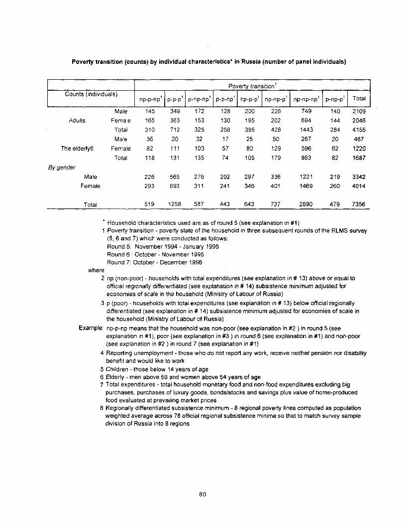
Poverty transition (counts) by individual characteristics* in Russia (number of panel individuals)

Poverty transition'Counts (individuals) np-p-np1 P-p-p1 p-np-np' p-p-np' Inp-p-p1 I np-np-pl np-np-npl p-np-p' Total

Male 145 349 172 128 200 226 749 140 2109Adults Female 165 363 153 130 195 202 694 144 2046

Total 310 712 325 258 395 428 1443 284 4155

Male 36 20 32 17 25 50 267 20 467

The elderly6 Female 82 111 103 57 80 129 596 62 1220

Total 118 131 135 74 105 179 863 82 1687

By gender

Male 226 565 276 202 297 336 1221 219 3342Female 293 693 311 241 346 401 1469 260 4014

Total 519 1258 587 443 643 737 2690 479 7356

Household characteristics used are as of round 5 (see explanation in #1)1 Poverty transition - poverty state of the household in three subsequent rounds of the RLMS survey

(5, 6 and 7) which were conducted as follows:Round 5: November 1994 - January 1995Round 6: October - November 1995Round 7: October- December 1996

where2 np (non-poor) - households with total expenditures (see explanation in # 13) above or equal to

official regionally differentiated (see explanation in # 14) subsistence minimum adjusted foreconomies of scale in the household (Ministry of Labour of Russia)

3 p (poor) - households with total expenditures (see explanation in # 13) below official regionallydifferentiated (see explanation in # 14) subsistence minimum adjusted for economies of scale inthe household (Ministry of Labour of Russia)

Example: np-p-np means that the household was non-poor (see explanation in #2 ) in round 5 (seeexplanation in #1), poor (see explanation in #3 ) in round 6 (see explanation in #1) and non-poor(see explanation in #2 ) in round 7 (see explanation in #1)

4 Reporting unemployment - those who do not report any work, receive neither pension nor disabilitybenefit and would like to work

5 Children - those below 14 years of age6 Elderly - men above 59 and women above 54 years of age7 Total expenditures - total household monetary food and non-food expenditures excluding big

purchases, purchases of luxury goods, bonds/stocks and savings plus value of home-producedfood evaluated at prevailing market prices

8 Regionally differentiated subsistence minimum - 8 regional poverty lines computed as populationweighted average across 78 official regional subsistence minima so that to match survey sampledivision of Russia into 8 regions

80

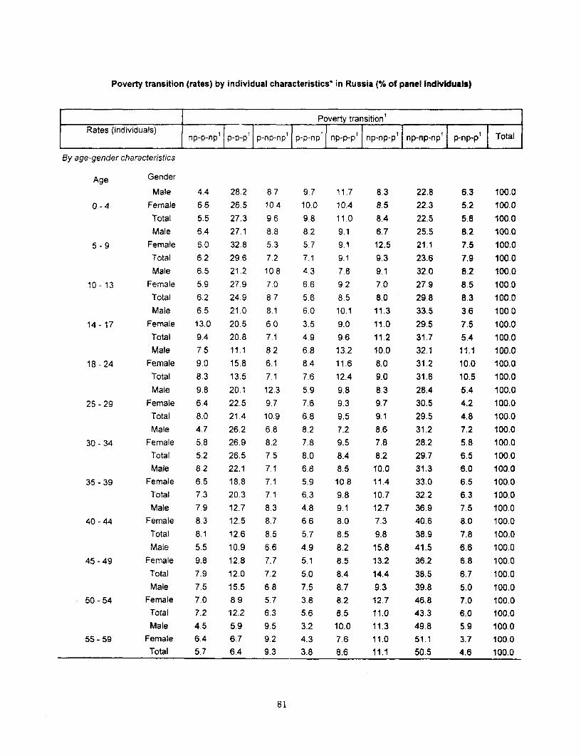
Poverty transition (rates) by individual characteristics' in Russia (% of panel individuals)

Poverty transition'

Rates (individuals) np-p-np1 p- p 1 p-np-np' p-p-np1 np-p-p' np-np-p' n-np-np' p-np-pI Total

By age-gender characteristics

Age GenderMale 4.4 28.2 8.7 9.7 11.7 8.3 22.8 6.3 100.0

0 -4 Female 6.6 26.5 10 4 10.0 10.4 8.5 22.3 5.2 100.0Total 5.5 27.3 9.6 9.8 11.0 8.4 22.5 5.8 100.0Male 6.4 27.1 8.8 8.2 9.1 6.7 25.5 8.2 100.0

5. 9 Female 6.0 32.8 5.3 5.7 9.1 12.5 21.1 7.5 100.0Total 6.2 29.6 7 2 7.1 9.1 9.3 23.6 7.9 1t0.0Male 6.5 21.2 10.8 4 3 7.8 9.1 32.0 8.2 100.0

10 - 13 Female 5.9 27.9 7 0 6.6 9.2 7.0 27.9 8.5 100.0Total 6.2 24.9 8.7 5.6 8.5 8.0 29.8 8.3 100.0Male 6.5 21.0 8.1 6.0 10.1 11.3 33.5 3.6 100.0

14- 17 Female 13.0 20.5 6.0 3.5 9.0 11.0 29.5 7.5 100.0Total 9 4 20.8 7.1 4.9 9.6 11.2 31.7 5.4 100.0Male 7.5 11.1 8.2 6.8 13.2 10.0 32.1 11.1 100.0

18 - 24 Female 9.0 15.8 6.1 8.4 11.6 8.0 31.2 10.0 100.0Total 8.3 13.5 7.1 7.6 12.4 9.0 31.6 10.5 100.0Male 9.8 20.1 12.3 5.9 9.8 8.3 28.4 5.4 100.0

25 - 29 Female 6.4 22.5 9.7 7.6 9.3 9.7 30.5 4.2 100.0Total 8.0 21.4 10.9 6.8 9.5 9.1 29.5 4.8 100.0Male 4.7 26.2 6.8 8.2 7.2 8.6 31.2 7.2 100.0

30 - 34 Female 5.8 26.9 8.2 7.8 9.5 7.8 28.2 5.8 100.0Total 5.2 26.5 7.5 8.0 8.4 8.2 29.7 6.5 100.0Male 8.2 22.1 7.1 6.8 8.5 10.0 31.3 6.0 100.0

35 39 Female 6.5 18.8 7.1 5.9 10.8 11.4 33.0 6.5 100.0Total 7.3 20.3 7.1 6.3 9.8 10.7 32.2 63 100.0Male 7.9 12.7 8.3 4.8 9.1 12.7 36.9 7.5 100.0

40 - 44 Female 8.3 12.5 8.7 6.6 8.0 7.3 40.6 8.0 100.0Total 8.1 12.6 8.5 5.7 8.5 9.8 38.9 7.8 100.0Male 5.5 10.9 6.6 4.9 8.2 15.8 41.5 6.6 100.0

45-49 Female 9.8 12.8 7.7 5.1 8.5 13.2 36.2 6.8 100.0Total 7.9 12.0 7.2 5.0 8.4 14.4 38.5 6.7 100.0Male 7.5 15.5 6.8 7.5 8.7 9.3 39.8 5.0 100.0

50 - 54 Female 7.0 8 9 5.7 3.8 8.2 12.7 46.8 7.0 100.0Total 7.2 12.2 6.3 5.6 8.5 11.0 43.3 6.0 100.0Male 4.5 5.9 9.5 3.2 10.0 11.3 49.8 5.9 100.0

S5 59 Female 6.4 6.7 9.2 4.3 7.6 11.0 51.1 3.7 100.0Total 5.7 6.4 9.3 3.8 8.6 11.1 50.5 4.6 100.0

81

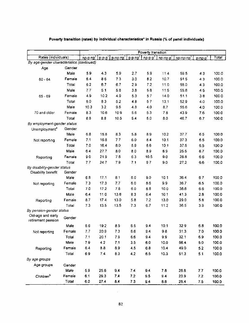
Poverty transition (rates) by Individual characteristics* in Russia (% of panel individuals)

I Poverty transition'Rates (individuals) I np-p-np' I p-p-p' p-np-np' I p-p-np' I np-2-p' I np-np-p1 I np-np-np' I p-np-p' I Total

By age-gender characteristics (continued)Age Gender

Male 5.9 4.3 5.9 2.7 5.9 11.4 59.5 4.3 100.060 - 64 Female 6.4 8.6 7.3 3.0 8.2 10.7 51.5 4.3 100.0

Total 6.2 6.7 6.7 2.9 7.2 11.0 55.0 4.3 100.0Male 7.7 5.1 5.8 3.8 5.8 11.5 55.8 4,5 100.0

65 - 69 Female 4.9 10.2 4.9 5.3 5.7 14.0 51.1 3.8 100.0Total 6.0 8.3 5.2 4.8 5.7 13.1 52.9 4.0 100.0Male 10.3 3.2 9.5 4.8 4.0 8.7 55.6 4.0 100.0

70 and older Female 8.3 10.6 10.9 5.6 5.3 7.8 43.9 7.6 100.0Total 8.8 8.8 10.5 5.4 5.0 8.0 46.7 6.7 100.0

By employment-gender statusUnemployment4 Gender

Male 6.8 15.8 8.3 5.8 8.9 10.2 37.7 6.5 100.0Not reporting Female 7.1 16.8 7.7 6.0 8.4 10.1 37.3 6.5 100.0

Total 7.0 16.4 8.0 5.9 8.6 10.1 37.5 6.5 100.0Male 6.4 27.7 8.0 8.0 8.9 8.9 25.5 6.7 100.0

Reporting Female 9.0 21.9 7.8 6.3 10.5 9.0 28.8 6.6 100.0Total 7.7 24.7 7.9 7.1 9.7 9.0 27.2 6.6 100.0

By disability-gender statusDisability benefit Gender

Male 6.8 17.1 8.1 6.0 9.0 10.1 36.4 6.7 100.0Not reporting Female 7.3 17.3 7.7 6.0 8.6 9.9 36.7 6.5 100.0

Total 7.0 17.2 7.8 6.0 8.8 10.0 36.6 6.6 100.0Male 6.4 11.0 13.8 8.3 6.4 10.1 41.3 2.8 100.0

Reporting Female 8.7 17.4 13.0 5.8 7.2 13.0 29.0 5.8 100.0Total 7.3 13.5 13.5 7.3 6.7 11.2 36.5 3.9 100.0

By pension-gender statusOld-age and early Genderretirement pension

Male 6.6 19.2 8.5 6.5 9.4 10.1 32.9 6.8 100.0Not reporting Female 7.7 20.9 7.3 6.6 9.4 9.8 31.3 7.0 100.0

Total 7.1 20.1 7.9 6.6 9.4 9.9 32.1 6.9 100.0Male 7.9 4.2 7.1 3.5 6.0 10.0 56.4 5.0 100.0

Reporting Female 6.4 8.8 8.9 4.5 6.8 10.4 49.0 5.2 100.0Total 6.9 7.4 8.3 4.2 6.5 10.3 51.3 5.1 100.0

By age groupsAge groups Gender

Male 5.9 25.6 9.4 7.4 9.4 7.8 26.8 7.7 100.0Children5 Female 6.1 29.3 7.4 7.2 9.5 9.4 23.9 7.2 100.0

Total 6.0 27.4 8.4 7.3 9.4 8.6 25.4 7.5 100.0

82

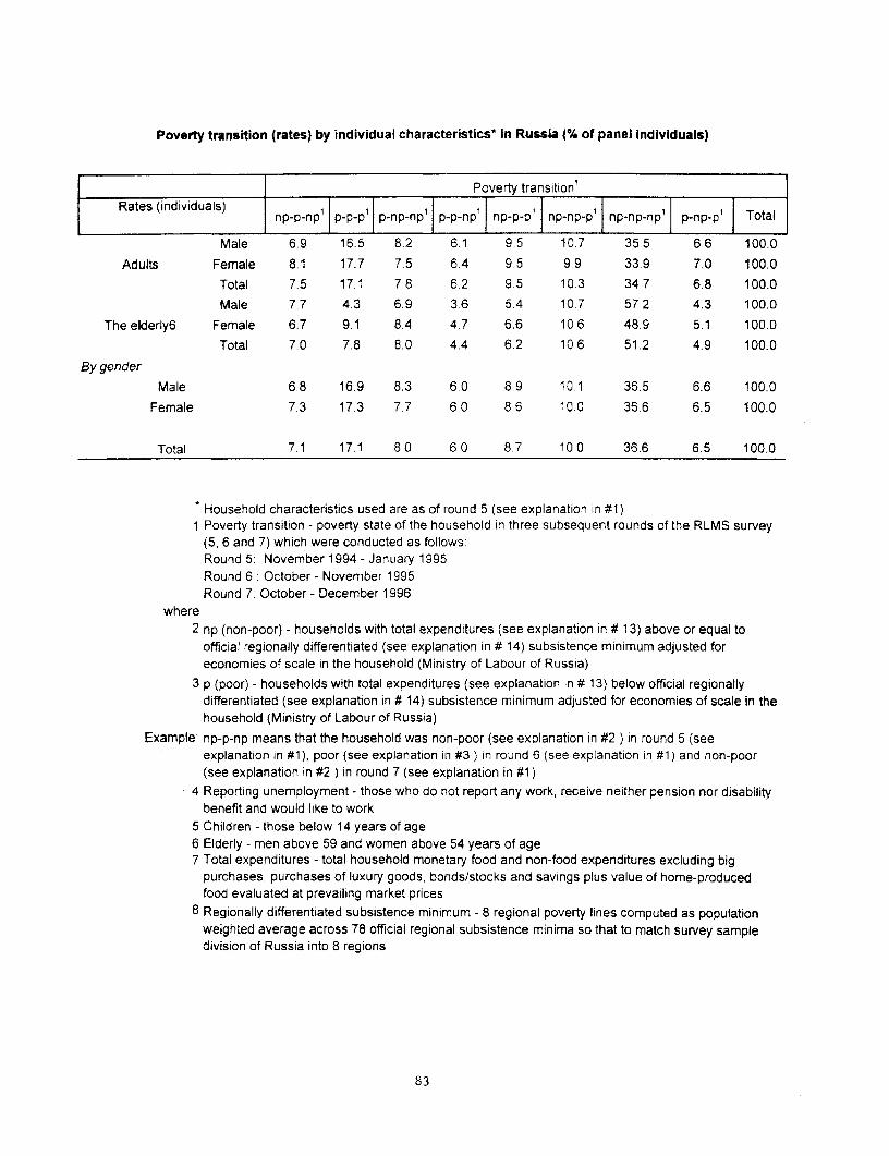
Poverty transition (rates) by individual characteristics* in Russia 4% of panel Individuals)

Poverty transition'Rates (individuals) 1 1 , l

np-p-np p-p-p p-np-np p-p-npl np-p-pl np-np-pl np-np-np1 p-np-pl Total

Male 6.9 16.5 8.2 6.1 9 5 10.7 35.5 6.6 100.0

Adults Female 8.1 17.7 7.5 6.4 9 5 9.9 33.9 7.0 100.0

Total 7.5 17.1 7.8 6 2 9 5 10.3 34.7 6.8 100.0

Male 7.7 4.3 6.9 3 6 5.4 10.7 57.2 4.3 100.0

The elderly6 Female 6.7 9.1 8.4 4.7 6.6 10.6 48.9 5.1 100.0

Total 7.0 7.8 8.0 4.4 6.2 10.6 51.2 4.9 100.0

By gender

Male 6.8 16.9 8.3 6.0 8.9 10.1 36.5 6.6 100.0

Female 7 3 17.3 7.7 6.0 8.6 10.0 36.6 6.5 100.0

Total 7 1 17 1 8.0 6 0 8 7 10 0 36.6 6.5 100.0

Household characteristics used are as of round 5 (see explanation in #1)1Poverty transition - poverty state of the household in three subsequent rounds of the RLMS survey

(5, 6 and 7) which were conducted as follows:Round 5. November 1994 - January 1995Round 6: October - November 1995Round 7 October - December 1996

where2 np (non-poor) - households with total expenditures (see explanation in # 13) above or equal to

official regionally differentiated (see explanation in # 14) subsistence minimum adjusted foreconomies of scale in the household (Ministry of Labour of Russia)

3 p (poor) - households with total expenditures (see explanation in # 13) below official regionallydifferentiated (see explanation in # 14) subsistence minimum adjusted for economies of scale in thehousehold (Ministry of Labour of Russia)

Example np-p-np means that the household was non-poor (see explanation in #2 ) in round 5 (seeexplanation in #1), poor (see explanation in #3 ) in round 6 (see explanation in #1) and non-poor(see explanation in #2 ) in round 7 (see explanation in #1)

4 Reporting unemployment - those who do not report any work, receive neither pension nor disabilitybenefit and would like to work

5 Children - those below 14 years of age6 Elderly - men above 59 and women above 54 years of age7 Total expenditures - total household monetary food and non-food expenditures excluding big

purchases, purchases of luxury goods, bonds/stocks and savings plus value of home-producedfood evaluated at prevailing market prices

8 Regionally differentiated subsistence minimum - 8 regional poverty lines computed as populationweighted average across 78 official regional subsistence minima so that to match survey sampledivision of Russia into 8 regions

83

Poverty transition (composition) by individual characteristics in Russia (% of panel individuals)

[T Poverty transition'

Composition (individuals) np-p-np' P-p-p p-np-np' p-p-np' np-p-p' np-np-p' np-np-np' p-np-p' Total

By age-gender characteristics

Age GenderMale 1.7 4.6 3.1 4.5 3.7 2.3 1.7 2.7 2.8

0 - 4 Female 2.7 4.5 3.7 4.7 3.4 2.4 1.7 2.3 2.9

Total 4.4 9 1 6.8 9.3 7.2 4.7 3.5 5.0 5.7

Male 4.0 7.1 4.9 6.1 4.7 3.0 3 1 5.6 4.5

5 9 Female 3.1 6.9 2.4 3.4 3.7 4.5 2.1 4.2 3.6

Total 7.1 14.0 7.3 9.5 8.4 7.5 5,2 9.8 8.1

Male 2.9 3.9 4.3 2.3 2.8 2.8 2.8 4.0 3.1

10- 13 Female 3.1 6.0 3.2 4.1 3.9 2.6 2.8 4.8 3.7

Total 6.0 9.9 7.5 6 3 6.7 5.4 5.6 8.8 6.8

Male 3.1 4.1 3.4 3.4 3.9 3.8 3.1 1.9 3.4

14- 17 Female 5.0 3.3 2.0 1.6 2.8 3.0 2.2 3.1 2.7

Total 8.1 7.4 5.5 5.0 6.7 6.8 5.3 5.0 6.1

Male 4.0 2.5 3.9 4.3 5.8 3.8 3.3 6.5 3.8

18 - 24 Female 5.4 3.9 3.2 5.9 5.6 3.4 3.6 6.5 4.2

Total 9.4 6.4 7.2 10.2 11.4 7.2 7.0 12.9 8.0

Male 3.9 3.3 4.3 2.7 3.1 2.3 2.2 2.3 2 8

25 - 29 Female 2.9 4.2 3.9 4.1 3.4 3.1 2.7 2.1 3.2Total 6.7 7.5 8.2 6.8 6.5 5.4 4.8 4.4 6.0

Male 2.5 5.8 3.2 5.2 3.1 3.3 3.2 4.2 3.8

30 34 Female 3.3 6.3 4.1 5.2 4.4 3.1 3.1 3.5 4.0Total 5.8 12.1 7.3 10.4 7.5 6.4 6.3 7.7 7.8

Male 4 4 4.9 3.4 4.3 3.7 3.8 3.3 3.5 3.8

35 39 Female 4.0 4 8 3.9 4.3 5.4 5.0 4.0 4.4 4.4

Total 8.5 9.8 7.3 8.6 9.2 8.8 7.2 7.9 8.2

Male 3.9 2.5 3.6 2.7 3.6 4.3 3.5 4.0 3.4

40 - 44 Female 4.6 2.9 4.3 4.3 3.6 2.8 4.3 4.8 3.9

Total 8.5 5.4 7.8 7.0 7.2 7.2 7.8 8.8 7.3

Male 1.9 1.6 2.0 2.0 2.3 3.9 2.8 2.5 2.5

45 -49 Female 4.4 2.4 3.1 2.7 3.1 4.2 3.2 3.3 3.2

Total 6.4 4.0 5.1 4.7 5.4 8.1 6.0 5.8 5.7

Male 2.3 2.0 1.9 2.7 2.2 2.0 2.4 1.7 2.2

50- 54 Female 2.1 1.1 1.5 1.4 2.0 2.7 2.8 2.3 2.1Total 4.4 3.1 3.4 4.1 4.2 4.7 5.1 4.0 4.3

Male 1.9 1.0 3.6 1.6 3.4 3.4 4.1 2.7 3.0

55 59 Female 4.0 1.7 5.1 3.2 3.9 4.9 6.2 2.5 4.4

Total 6.0 2.8 8.7 4.7 7.3 8.3 10.3 5.2 7.4

84

Poverty transition (composition) by individual characteristics* in Russia (% of panel individuals)

Poverty transition'Composition (individuals) np-p-np1 p-p-pI p-np-np' p-p-np' np-p-p' np-np-p' np-np-npl p-np-p' Total

By age-gender characteristics (continued)Age Gender

Male 2.1 0.6 1.9 1.1 1.7 2.8 4 1 1.7 2.5

60 - 64 Female 2.9 1.6 2.9 1.6 3.0 3.4 4.5 2.1 3 2Total 5 0 2.2 4.8 2.7 4 7 6.2 8.6 3.8 5 7

Male 2.3 0.6 1.5 1 4 1 4 2 4 3.2 1.5 2.1

65-69 Female 2.5 21 22 32 2.3 50 5.0 2.1 3.6Total 4.8 2.8 3.7 4.5 3.7 7 5 8.3 3 5 5.7Male 25 0.3 2.0 1.4 0 8 1.5 2.6 1 0 1.7

70 and older Female 6.4 3.3 7.3 5.0 3 3 4.2 6.5 6.3 5 4Total 8.9 3.7 9 4 6.3 4 0 5.7 9.1 7.3 7.1

Total 100.0 100.0 100 0 100.0 100.0 100 0 100.0 100.0 100.0By employment-gender status

Unemployment4 Gender

Male 39.7 38.0 42.8 40.0 41.8 41.8 42.4 41 3 41.2

Not reporting Female 50.7 49.3 48.6 49.7 48.4 50.3 51.0 49.7 50.0Total 90.4 87.3 91.3 89.6 90.2 92.1 93.5 91.0 91.2Male 3.9 6.9 4.3 5.6 4.4 3.8 3.0 4.4 4.3

Reporting Female 5.8 5.8 4.4 4.7 5.4 4.1 3 6 4.6 4.5Total 9.6 12.7 8.7 104 98 79 65 9.0 8.8

Total 100.0 100.0 100.0 100.0 100.0 100.0 100 0 100.0 100 0

By disability-gender statusDisability benefit Gender

Male 42.2 44.0 44.5 43.6 45.1 44.1 43.7 45.1 44 0Not reporting Female 55.3 54.1 51 4 53 5 53.0 53.2 53 9 53.4 53.6

Total 97.5 98.1 95 9 97.1 98.1 97.3 97.6 98.5 97.6Male 1.3 1.0 2.6 2.0 1.1 1.5 1.7 0.6 1.5

Reporting Female 1 2 1 0 1.5 0 9 0 8 1.2 0.7 0.8 0.9Total 2.5 1.9 4 1 2.9 1.9 2.7 2.4 1.5 2.4

Total 100 0 100 0 100.0 100 0 100 0 100.0 100.0 100 0 100.0By pension-gender status

Old-age and early Genderretirement pension

Male 35 6 43 2 40.7 41.5 41.4 38.5 34.5 40.3 38.3

Notreporting Female 41.6 46 7 34 9 42 2 41 2 37.4 32.8 41.3 38.3Total 77 3 89 9 75 6 83 7 82.6 76.0 67.2 81.6 76.6Male 7.9 1.7 63 4.1 48 7 1 10.9 5.4 7.1

Reporting Female 14.8 8.3 18.1 12.2 12.6 17.0 21.8 12.9 16.3Total 22.7 10.1 24.4 16.3 17.4 24.0 32.8 18.4 23.4

Total 100.0 100.0 100.0 100.0 100.0 100.0 100.0 100.0 100.0

85

Poverty transition (composition) by individual characteristics* in Russia (% of panel individuals)

I Poverty transitionlComposition (individuals) np-p-np' |p-p-p' -p | np-nEn- | p-np-pT Total

By age groups

Age groups Gender

Male 8.7 15.6 123 12.9 112 8.1 76 123 104

C:hildren5 Female 8,9 17.4 9 4 12 2 11 0 9.5 6,7 11,3 10.2Total 17.5 33.0 21.6 25 1 22.2 176 14.3 236 20.6

Male 27.9 27.7 29.3 28 9 311 30 7 27.8 29 2 28.7

Adults Female 31 8 28.9 26.1 29 3 30.3 27.4 25.8 30 1 27.8

Total 59.7 56.6 554 58 2 61 4 58.1 53 6 59 3 56,5

Male 6.9 1.6 5 5 3 8 3 9 6 8 9 9 4 2 6 3

The elderly6 Female 15 8 8.8 175 12 9 12 4 175 22,2 12 9 16.6

Total 227 10.4 23.0 16.7 163 24 3 32.1 171 22.9

Total 100.0 100 0 100 0 100.0 100C0 100,0 100 0 100.0 100.0

By gender

Male 43.5 449 470 456 462 45.6 454 457 454

Female 56 5 55 1 53.0 54 4 53 8 54.4 546 54.3 54.6

Total 100.0 100.0 1000 100.0 1000 100.0 100.0 1000 1000

Household characteristics used are as of round 5 (see explanation in #1)1 Poverty transition - poverty state of the household in three subsequent rounds of the RLMS survey

(5, 6 and 7) which were conducted as follows.

Round 5: November 1994 - January 1995Round 6: October - November 1995Round 7: October- December 1996

where2 np (non-poor) - households with total expenditures (see exp anation in # 13) above or equal to

official regionally differentiated (see explanation in # 14) subsistence minimum adjusted foreconomies of scale in tne household (Ministry of Labour of Russia)

3 p (poor) - households with total expenditures (see explanation in # 13) below official regionallydifferentiated (see explanation in # 14) subsistence minimum adjusted for economies of scale in thehousehold (Ministry of Labour of Russia)

Example. np-p-np means that the household was non-poor (see explanation in #2 ) in round 5 (seeexplanation in #1) poor (see explanation in #3 ) in round 6 (see explanation in #1) and non-poor(see explanation in #2 ) in round 7 (see explanation in #1)

4 Reporting unemployment - those who do not report any work, receive neither pension nor disabilitybenefit and would like to work

5 Children - those below 14 years of age6 Elderly - men above 59 and women above 54 years of age7 Total expenditures - total household monetary food and non-food expenditures excluding big

purchases, purchases of luxury goods, bonds/stocks and savings plus value of home-produced foodevaluated at prevailing market prices

8 Regionally differentiated subsistence minimum - 8 regional poverty lines computed as populationweighted average across 78 official regional subsistence minima so that to match survey sampledivision of Russia into 8 regions

86

ANNEX FOUR

PROXY MEANS TESTS FOR RUSSIA 1994-98

JEANINE BRAITHWAITE (ECSPE)

ANNA IVANOVA (U.WISC.)

1. A proxy means test is a method to estimate household consumption or welfarewithout requiring extremely detailed information about household income. In countriessuch as Russia or Chile where there is a large informal sector, it can be very difficult andadministratively very costly to verify true household money income. Furthermore, inRussia and other countries, a very significant part of household food consumption comesfrom food grown on private garden plots. It can be very difficult to estimate the true value(impute the value correctly) of home-produced goods, since typically, they are producedwith "costless" family labor and their quality may be different than for example fooditems which are produced for sale.

2. In proxy means tests, rather than trying to measure total income perfectly,information is collected on items which are much easier to measure and verify, such as thenumber of children in the family, etc. These variables should be ones which are known tocorrelate with poverty in the country, and ideally, which are easy to measure and thusrequire little administrative cost to verify. The first large-scale use of proxy means-testingoccurred in Chile in the late 1970s and 1980s, in a program called the Ficha CAS (card forsocial assistance). Since 1994, Costa Rica and Columbia have adopted proxy means-testsfor some of their social assistance programs, Mexico is about to start a proxy means-testprogram, and Argentina and Venezuela are actively considering the idea.

3. Within the region, independently of the Latin American experience, Armenia hasadopted a proxy means test in its Paros program for the distribution of humanitarianassistance. However, the scoring formula used in the Paros program was not based on anysort of econometric estimates and may contain some inaccuracies. Rather than use thescoring formula of the Paros program for Russia, it would be much better to estimate anew scoring formula. Indeed, in each country usinlg a proxy means test, a unique scoringformula is estimated, based on data on household expenditures and characteristics.

4. This paper presents several different proxy means regressions for Russia or oblastsof Russia. Results differed for many reasons, the most important of which were the highlydifferent sources of data used and the different time periods to which the regressionspertained. Furthermore, the results are presented in chronological order, from the veryfirst proxy means test results for data from early 1994 of the RLMS (these data are notuised elsewhere in this report), through social assistance pilot data for 1997-98, and finally,for the three rounds of the World Bank version of the RLMS data set for 1994-96.

I

1. SIMULATION FOR RUSSIA AND VOLGOGRAD

5. A data base is required for estimating an appropriate scoring formula for Russia.For this first illustrative example, household data for Russia for October 1993-February1994 (Round IV) from the Russian Longitudinal Monitoring Survey (RLMS) are used.

6. The first step in any study of household behavior is to decide on a best measure ofhousehold consumption, which is usually considered to be household expenditures plusthe market value of any goods produced and consumed by the household.' Here we facethe first technical limitation of Round IV of the RLMS. Unlike Rounds l-II, in Round IVhouseholds were asked only one question about the value of goods (mostly food) producedand consumed at home--they were asked to estimate its worth. In other householdsurveys, such as one done in Ukraine in 1995 and 1996, households were asked to providedetails about their food production & consumption in physical units by each type of food.and then survey researchers imputed the value of the food (by using average purchaseprices). This approach will also be used in the survey of the social assistance pilots, sinceit produces much more reliable estimates of household production and consumption offood. Preliminary work with the Round IV data of the RLMS suggest that householdsmay have under-estimated the value of the food they produced on their own private plots,perhaps in many cases because the household simply did not know the correct marketprice for its food.

7. For this illustrative example, however, it was not possible to adjust or correct theRound IV results, so they will be used with caution. Thus the measure of householdwelfare used here is total household expenditures, which include the household's ownestimate of the value of food and other goods it produced and consumed and the value ofall household reported purchases of food, non-food goods. services, and miscellaneousother purchases. Total household expenditures are then divided by the number ofhousehold members to generate per capita expenditures.2 Thus below per capita isunderstood to be "per household member."

8. The next step was to try to measure the correlation between household welfare (percapita expenditures) and other easily-measured variables. The technique used wasstepwise least squares regression, in which variables are excluded if they are notsignificantly correlated with per capita expenditures. Technically speaking, this techniqueshould only be used for variables which are thought to be independent (exogenous) andnot directly correlated with each other. I-lowever, since we are only trying to find proxies

Although many statistical publications rely on houschold income as measure of household welfare, there aremany studies which demonstrate that if household cxpenditurc data are available, they should be used inpreference to data on household income, whichl tenlds to bc under-reported, especially on the high end of theincome distribution. Household income tends to appear frequently in statistical publications of manycountries because typically, monthly estimates of household income are made by central statistical agencies,while household expenditures data are more commonily available on an annual (or sometimes quarterly)basis.

2 There is an extremely lively debate in the economics literature about whether per capita measurements are asdesirable as "equivalent adult" measurements which reflect economies of scale in consumption (decliningmarginal cost of additional family members), but for the purposes of the pilot, we will set aside this debate.

2

(substitutes) for poverty which are more easily measured than household expenditures(rather than trying to decide what determines poverty) we can ignore this caveat in thiscontext. Especially, we will ignore the caveat because we will regress per capitaexpenditures on a variety of variables, including official money income (wages plustransfer payments such as pensions, allowances, and stipends).3

9. During the first round of regressions, some surprising and possibly doubtful resultsoccurred. For example, the presence of a female household head4 seemed to correlate withhigher levels of per capita expenditures than those of a male household head, while thepresence of a private plot seemed to reduce the level of per capita expenditures. The firstresult may have occurred because there are few female household heads and they may beable to estimate more accurately their expenditures. The second result undoubtedlyreflects the technical limitation about self-production from the questionnaire noted above.Since it is possible to spend a very long time on econometric work without resolvingissues of this sort, it was decided to simply drop variables that seemed to have aproblematic relationship to per capita expenditures, even if the variable seemed to besignificantly correlated with per capita expenditures.

10. The final specification is one in which all the coefficients estimated are significantat the 10 percent level, and all but one are extremely significant. We estimated

C = a + bY + cX

where C is per capita expenditures (exp_p in the table below)

Y is per capita official income (jbmi_p in the table below, consisting of the sum ofhousehold wage income and transfer income, including pensions, child allowances,stipends, local social assistance, unemploymenlt benefits, and other cash and in-kindtransfers)'

Xi is a set of other easily measured variables, including the number of children inthe family (CHILDN), the number of elderly (ELDERLYN). whether the household islocated in a city other than Moscow (DLOC I), whether the household is a rural household(DLOC2),6 whether the household has a refrigerator (RREFIGDA), whether the

In this sense, we are estimating a houiselhold consumption function, where C = a + bY + cX, where C isconsumption (as measured by per capita expenditures), Y is per capita money income, and X, is a vector ofindependent variables independent from income. However. since in practice most of our easily measured X,variables are not likely to be completely independent from income, we would be violating one of therequirements of the regression model if we were seeking to determine causality.

4A female headed household was defined as one in which there was an active-aged female (over 15 and under 55)but no active-aged male or a household in which there were no active-aged adults, an elderly female but noelderly male.

5For in-kind transfers, this represents the estimate of the person answering the questionnaire on the value of thein-kind transfer. For wages, respondents were asked to estimate the monetary value of any wages paid in-kind.

6 In this definition, villages of the urban type are classified as rural.

3

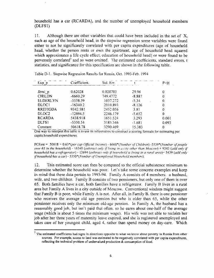
household has a car (RCARDA), and the number of unemployed household members(DLFS1)

It. Although there are other variables that could have been included in the set of Xisuch as age of the household head, in the stepwise regression some variables were foundeither to not be significantly correlated with per capita expenditures (age of householdhead, whether the person rents or own the apartment, age of household head squaredwhich approximates a life cycle effect, education of household head) or were found to beperversely correlated' and so were omitted. The estimated coefficients, standard errors, tstatistics, and significance for this specification are shown in the following table.

Table D-1. Stepwise Regression Results for Russia, Oct. 1993-Feb. 1994

Expp Coefficient. Std. Err. t P>ltJ

Jbmi_p 0.62028 0.020703 29.96 0CHILDN -6660.29 749.4772 -8.887 0ELDERLYN -5538.59 1037.272 -5.34 0DLOCI -16340.2 2010.893 -8.126 0RREFIGDA 9342.581 2452.056 3.81 0DLOC2 -12694.5 2246.179 -5.652 0RCARDA 5438.918 1651.524 3.293 0.001DLFSI -5350.54 3183.346 -1.681 0.093Constant 50618.78 3290.469 15.383 0

One way to interpret this table is to use its information to construct a scoring formula for estimating percapita household expenditures.

PCEest = 50618 + 0.63*(per cap Official Income) - 6660*(Numnher c?f Children) -5539*(Numher of peopleover 65 in the household) - 16340 (suibtr-act only if living in a city other than Moscow) + 9343 (add onb' ijhousehold has a refrigerator) - 12694 (subtract only if household is living in a rueral area)+ 5439 (add onlyif household has a car) - 5350*(Nu,mber of UneinploVed Hlousehold mnembers).

12. This estimated score can then be compared to the official subsistence minimum todetermine whether the household was poor. Let's take some concrete examples and keepin mind that these data pertain to 1993-94. Family A consists of 4 members: a husband,wife, and two children. Family B consists of two pensioners, but only one of them is over65. Both families have a car, both families have a refrigerator. Family B lives in a ruralarea but Family A lives in a city outside of Moscow. Conventional wisdom might suggestthat Family B is poor, while Family A is not. After all, in Family B, there is one pensionerwho receives the average old age pension but who is older than 65, while the otherpensioner receives only the minimum old-agc pension. In Family A, the husband has areasonably good job, but isn't paid that often, so he earns about one-half of the averagewage (which is about 5 times the minimum wage). His wife was not able to reclaim herjob after her three years of maternity leave expired, and she is registered unemployed andtakes care of her youngest child, aged 4, rather than spend money on day-care. Which

7 The estimated coefficients had signs in directions opposite to what we know about poverty in Russia from othersources. For example, access to land was estimated to be negatively correlated with per capita expenditures,reflecting the technical problem of undervalued production & consumption of food.

4

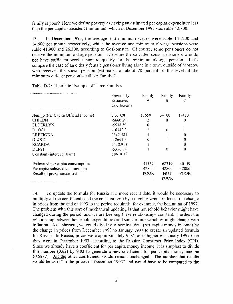
family is poor? Here we define poverty as having an estimated per capita expenditure lessthan the per capita subsistence minimum, which in December 1993 was ruble 42,800.

13. In December 1993, the average and minimum wages were ruble 141.200 and14,600 per month respectively, while the average and minimum old-age pensions wereruble 41,900 and 26,300, according to Goskomstat. Of course, some pensioners do notreceive the minimum old-age pension. These are the so-called social pensioners who donot have sufficient work tenure to qualify for the minimum old-age pension. Let'scompare the case of an elderly female pensioner living alone in a town outside of Moscowwho receives the social pension (estimated at about 70 percent of the level of theminimum old-age pension)--call her Family C.

Table D-2: Heuristic Example of Three Families

Previously Family Faim ily FamilyEstimated A B CCoefficients

Jbmi_p (Per Capita Official Income) 0.62028 17650 34100 18410CHILDN -6660.29 2 0 0ELDERLYN -5538.59 0 1 1DLOCI -16340.2 1 0 1RREFIGDA 9342.581 1 1 0DLOC2 -12694.5 0 1 0RCARDA 5438.918 1 1 0DLFS1 -5350.54 1 0 0Constant (intercept term) 50618.78

Estimated per capita consumption 41337 68319 40159Per capita subsistence miiiinimuI 42800 42800 42800Result of proxy means test POOR NOT POOR

POOR

14. To update the formula for Russia at a more recent date, it would be necessary tomultiply all the coefficients and the constant term by a number which reflected the changein prices from the end of 1993 to the period required: for example, the beginning of 1997.The problem with this sort of mechanical updating is that household behavior might havechanged during the period, and we are keeping these relationships constant. Further, therelationship between household expenditures and some of our variables might change withinflation. As a shortcut, we could divide our nominal data (per capita money income) bythe change in prices from December 1993 to January 1997 to create an updated formulafor Russia. In Russia, prices were approximately 9.02 times higher in January 1997 thanthey were in December 1993, according to the Russian Consumer Price Index (CPI).Since we already have a coefficient for per capita money income, it is simplest to dividethis number (0.62) by 9.02 to generate a new coefficient for per capita money income(0.6877). All the other coefficients would remain unchanged. The number that resultswould be as if "in the prices of December 1993" and would have to be compared to the

5

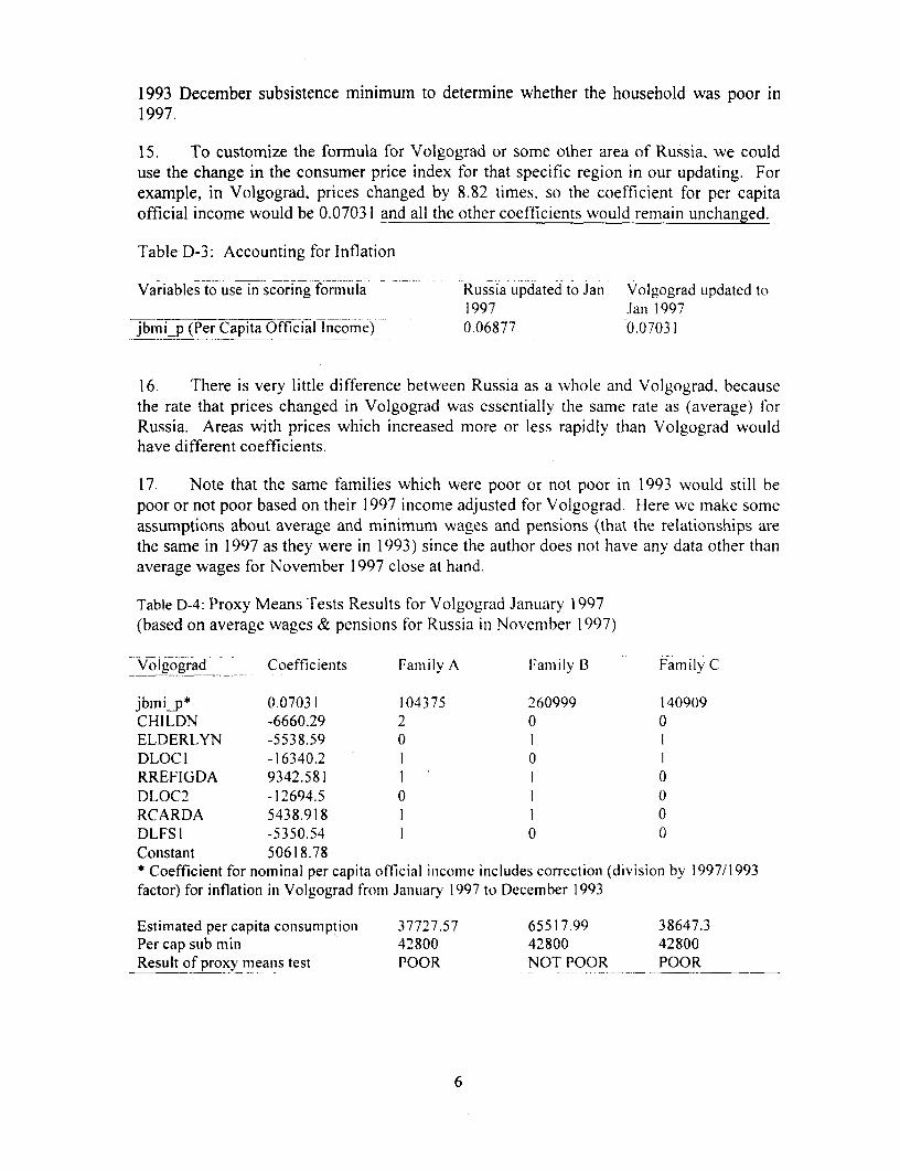
1993 December subsistence minimum to determine whether the household was poor in1997.

15. To customize the formula for Volgograd or some other area of Russia. we coulduse the change in the consumer price index for that specific region in our updating. Forexample, in Volgograd, prices changed by 8.82 times, so the coefficient for per capitaofficial income would be 0.07031 and all the other coefficients would remain unchanged.

Table D-3: Accounting for Inflation

Variables to use in scoring formula Russia updated to Jan Volgograd updated to1997 Jan 1997

jbmi_p (Per Capita Official Income) 0.06877 0.07031

16. There is very little difference between Russia as a whole and Volgograd, becausethe rate that prices changed in Volgograd was essentially the same rate as (average) forRussia. Areas with prices which increased more or less rapidly than Volgograd wouldhave different coefficients.

17. Note that the same families which were poor or not poor in 1993 would still bepoor or not poor based on their 1997 income adjusted for Volgograd. Here we make someassumptions about average and minimum wages and pensions (that the relationships arethe same in 1997 as they were in 1993) since the author does not have any data other thanaverage wages for November 1997 close at hand.

Table D-4: Proxy Means Tests Results for Volgograd J.anuary 1997(based on average wages & pensions for Russia in November 1997)

Volgograd Coefficients Family A Faillily B Family C

jbmi_p* 0.07031 104375 260999 140909CHILDN -6660.29 2 0 0ELDERLYN -5538.59 0 1 1DLOCI -16340.2 I 0 1RREFIGDA 9342.581 1 I 0DLOC2 -12694.5 0 1 0RCARDA 5438.918 1 1 0DLFSI -5350.54 1 0 0Constant 50618.78* Coefficient for nominal per capita official incomiie includes correction (division by 1997/1993factor) for inflation in Volgograd fromii Janulary 1997 to December 1993

Estimated per capita consumption 37727.57 65517.99 38647.3Per cap sub min 42800 42800 42800Result of proxy means test POOR NOT POOR POOR

6

II. SOCIAL ASSISTANCE PILOT PRELIMINARY RESULTS

18. Very preliminary results of the targeting experiments conducted in three oblasts ofRussia in 1998 as part of the Government's social reform program, supported by theWorld Bank through the Social Protection Adjustment Loan (SPAL). are available andused below. However, these data were obtained to early in the project cycle to be trueestimates of the targeting potential of the three methods tested. The final wave of fieldwork was conducted in September 1998 and data are being cleaned and processed. Thesedata will be ready at the end of November. and the simulations in this section will beupdated.

19. In each of the three pilots, household per capita income or per capita potential orestimated income or consumption was compared to the regional poverty line. Theregional poverty line was based on the Ministry of Labor methodology and local prices, asreported to the social assistance pilots team. The eligibility thresholds were a percentageof the per capita regional poverty line (50 percent in Volgograd and Voronezh, 35 percentin Komi).

20. In Komi, the methodology was said to determine the "Economic Potential" of ahousehold. In Voronezh, the methodology was intended to estimate the potential totalincome (sovokupniy dokhod) of a household. In Volgograd, the clients were informedthat their eligibility would depend on their "potential consumption." Although the namesdiffered, the mechanics of each methodology were fairly similar. Based on informationsubmitted by households on their official (wage plus transfer) income, demographiccharacteristics, and durable goods and/or assets, each methodology in essence tried toestimate how much more the household was or could consume than its reported income.

21. For example, in Komi, the "'module of economic potential" valuation depended toa great deal on whether or not the household had an imported or other automobile orexcess living space (more space than the 'norm'), based on assumptions and hidden expertvaluations. This potential income was added to the household's reported income todetermiiine eligibility. In Voronezh, an agricultural area, the methodology was intended toestimate agricultural income, based on the household inventory of livestock. Expertvaluation was used to generate average prices for the various kinds of livestock.

22. Volgograd was the only methodology that was openly derived from householdsurvey data. Using annual data for 1996, household per capita consumption wascalculated, then estimated by step-wise linear regression analysis. The correlationsbetween consumption and variables (estimated beta coefficients) such as the number ofchildren or whether the household had a private plot of land were estimated. Thesecorrelations were then used in a formula (which was updated for inflation) to determineestimated household consumption.

23. It seems that the actual methodologies employed in the three pilot oblasts were aseffective in identifying the poor as simulations performed. Based on the criteria of 1/2 ofthe subsistence minimum in Volgograd and Voronezh, and 35 percent (also called GDD)in Komi, the non-poor were rather well identified by the pilots in practice, and the poor

7

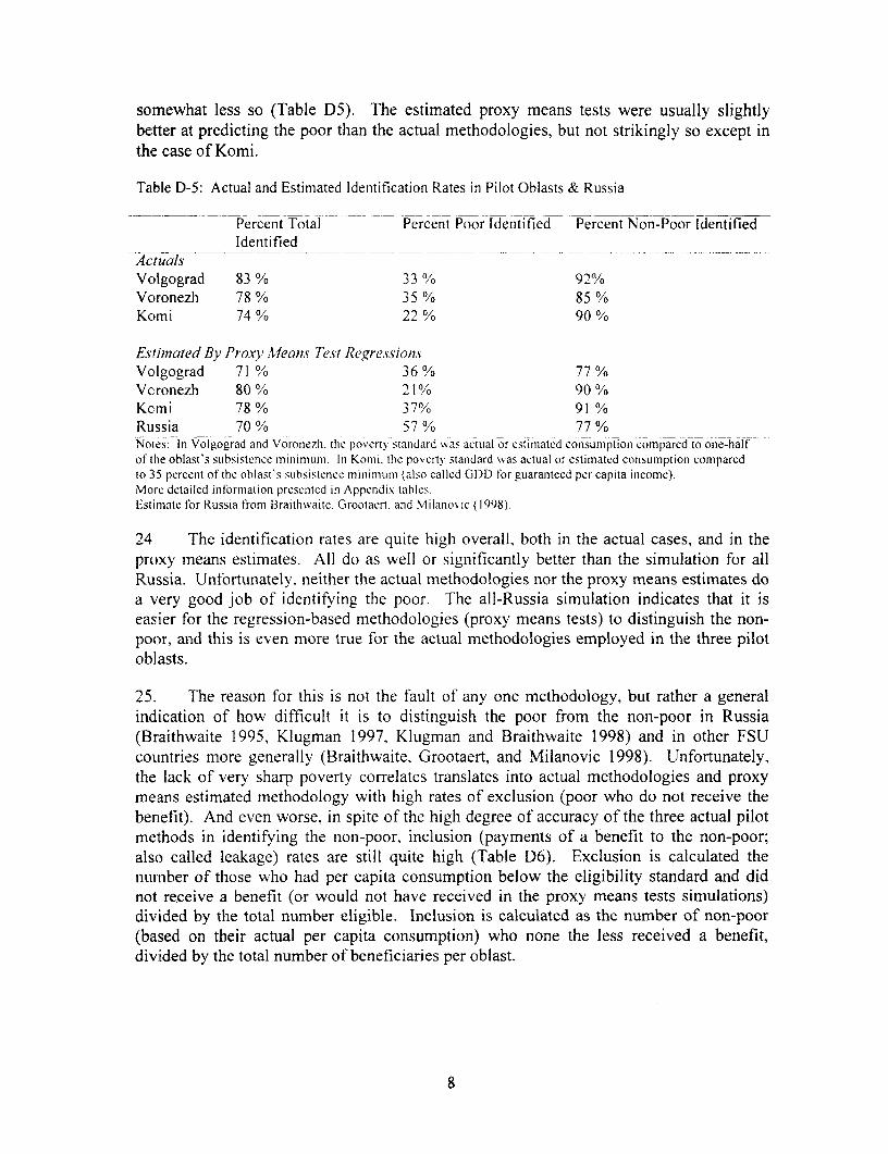
somewhat less so (Table D5). The estimated proxy means tests were usually slightlybetter at predicting the poor than the actual methodologies, but not strikingly so except inthe case of Komi.

Table D-5: Actual and Estimated Identification Rates in Pilot Oblasts & Russia

Percent Total Percent Poor Identified Percent Non-Poor IdentifiedIdentified

ActualsVolgograd 83 °/0 33 % 92%Voronezh 78 % 35 % 85 %Komi 74 % 22 % 90 %

Evs,rimaed By Proxv Means Test RegressionisVolgograd 71 % 36% 77%Vcronezh 80 % 21% 90 %Kcmi 78 % 37% 91 %Russia 70 % 57 % 77 %Notes: In Volgograd and Voronezh. the poverty standard x% as actual orestimated consumption compared to one-halfof the oblast's subsistence minimum. In Komi. the poverty standard was actual or estimated consumption comparedto 35 percent of the oblast's subsistence minimumri (also called GDD for guaranteed per capita income).More detailed inobrmation presentcd in Appendix tabics.Estimate for Russia from Braithwaite, Grootaert, and Milanovic (1998).

24. The identification rates are quite high overall, both in the actual cases, and in theproxy means estimates. All do as well or significantly better than the simulation for allRussia. Unfortunately, neither the actual methodologies nor the proxy means estimates doa very good job of identifying the poor. The all-Russia simulation indicates that it iseasier for the regression-based methodologies (proxy means tests) to distinguish the non-poor, and this is even more true for the actual methodologies employed in the three pilotoblasts.

25. The reason for this is not the fault of any one methodology, but rather a generalindication of how difficult it is to distinguish the poor from the non-poor in Russia(Braithwaite 1995, Klugman 1997, Klugman and Braithwaite 1998) and in other FSUcountries more generally (Braithwaite, Grootaert, and Milanovic 1998). Unfortunately,the lack of very sharp poverty correlates translates into actual methodologies and proxymeans estimated methodology with high rates of exclusion (poor who do not receive thebenefit). And even worse, in spite of the high degree of accuracy of the three actual pilotmethods in identifying the non-poor, inclusion (payments of a benefit to the non-poor;also called leakage) rates are still quite high (Table D6). Exclusion is calculated thenurnber of those who had per capita consumption below the eligibility standard and didnot re.ceive a benefit (or would not have received in the proxy means tests simulations)divided by the total number eligible. Inclusion is calculated as the number of non-poor(based on their actual per capita consumption) who none the less received a benefit,divided by the total number of beneficiaries per oblast.

8

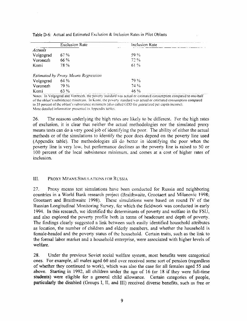
Table D-6: Actual and Estimated Exclusion & Inclusion Rates in Pilot Oblasts

Exclusion Rate Inclusion RateActualsVolgograd 67 % 59 %Voronezh 66 % 72 %Komi 78% 610%

Estitnated by Proxy Means RegressioniVolgograd 64 % 79 %Voronezh 79 % 74 %Komi 63 % 46 %Notes: In Volgograd and Voronezhi, thc povcrto stanidard was actual or estimated conlsumilptioIn compared to one-hal-oi'thc oblast's subsistcnce minilum. In Koomi. the povertx standard was actual or estimated consumption comparedto 35 percent of the oblast's subsistence minimulLIm (also called GDD for guaranteed per capita income).More detailed information presenited in Appeindix tables.

26. The reasons underlying the high rates are likely to be different. For the high ratesof exclusion, it is clear that neither the actual methodologies nor the simulated proxymeans tests can do a very good job of identifying the poor. The ability of either the actualmethods or of the simulations to identify the poor does depend on the poverty line used(Appendix table). The methodologies all do better in identifying the poor when thepoverty line is very low, but performance declines as the poverty line is raised to 50 or100 percent of the local subsistence minimum, and comes at a cost of higher rates ofinclusion.

III. PROXY MEANS SIMULATIONS FOR RuSSIA

27. Proxy means test simulations have been conducted for Russia and neighboringcountries in a World Bank research project (Braithwaite, Grootaert and Milanovic 1998;Grootaert and Braithwaite 1998). These simulations were based on round IV of theRussian Longitudinal Monitoring Survey, for which the fieldwork was conducted in early1994. In this research, we identified the determinants of poverty and welfare in the FSU,and also explored the poverty profile both in terms of headcount and depth of poverty.The findings clearly suggested a link between such easily identified household attributesas location, the number of children and elderly members, and whether the household isfemale-headed and the poverty status of the household. Certain traits, such as the link tothe formal labor market and a household enterprise, were associated with higher levels ofwelfare.

28. Under the previous Soviet social welfare system, most benefits were categoricalones. For example, all males aged 60 and over received some sort of pension (regardlessof whether they continued to work), which was also the case for all females aged 55 andabove. Starting in 1992, all children under the age of 16 (or 18 if they were full-timestudents) were eligible for a general child allowance. Certain categories of people,particularly the disabled (Groups I, II, and III) received diverse benefits, such as free or

9

reduced-price utilities and transportation services. Universal benefits such as generalizedconsumer subsidies were removed in the course of stabilization programs. but may havetainted some of the categorical programs as well.

29. Since many of those who received such categorical benefits were demonstrated toactually be the non-poor (see various World Bank poverty assessments) while universalconsumer subsidies were shown to be fiscally unsustainable and highly inequitable.categorical targeting received significant and warranted criticism from external andinternal advisors and policy makers. However, the problem with categorical targetingmay have been in the poor choice of categories more so than the idea of using an indicatoror combination of indicators (a proxy means test) to identify the poor. The choice ofcategories was dictated by political considerations (relating to the labor theory of valueand whether a person was perceived as being able to work or not). not by a careful studyof who was poor and what determined poverty.

30. In this section, we try to determine whether a combination of indicators canidentify the poor, which in turn would provide the necessary information for effectivetargeting of cash or in-kind benefits, or for active labor market policies. In practice, in theFSU, and particularly in Russia and Ukraine. increasingly benefits are being awarded toapplicants who meet a categorical filter amd an income-test. Typically. this means-test isbased only on official income. Unfortunately in the FSU. official income alone is aparticularly poor predictor of household welfare, due to the pervasive informal sector andthe general unwillingness of households to disclose such sensitive information.

31. Preliminary evidence from the housing allowance subsidy programs in Ukraineand Russia, which are based on official income (wages plus transfer income) suggest thatthis official income-test has a very high error of exclusion (those who are actually poor arenot receiving the benefit). Partly this originates from the very different goal of theseprograms, which is to promote housing privatization, and partly it may originate from alack of consideration of other factors related to poverty which are not captured in officialincome.

32. In order to improve means-testing where it currently exists, and to revise andupdate the categorical approach overall, we estimate an expanded welfare equation withvariables added for official income (wages and social transfers) and for ownership ofhousehold durable. Owing to the obvious endogeneity of these variables, no causalinterpretation should be assigned to the coefficients. The sole purpose here is to determinetheir predictive power. All of the regresses included (household durable, official income,family composition/demographic characteristics, location, unemployment status) are allfairly easy to identify by social workers, either through direct observation, declaration, orverification through documentation or a home visit. The model was estimated withforward stepwise regression.

33. The data in Table D-7 show that the proxy means test was able to identify correctlyapproximately 65-75 percent of the populations, with all three countries having betterpredictions for the non-poor than for the poor. Only about 60 percent (57-62) of the poorwere identified correctly, but this still represent a significant improvement over the

10

previous single-indicator/categorical approach used to allocate benefits such as old-agepensions and student stipends.8

34. At first glance, the five best predictors for the FSU countries seem to be morerelated to the non-poor side of the spectrum (wage income, car, color TV, householdbusiness, university education, land ownership) as to the poor (transfer income). Even so,the five best predictors achieved almost the same degree of accuracy as did the completemodel, identifying only slightly less of the poor (54-57 percent) and the populations (64-70 percent). Even the addition of the next five (best ten total) predictors shows a mixtureof factors associated with higher welfare (stereo, car, household enterprise) as with lowwelfare (number of children. transfer income, rural location, other urban location, numberof unemployed, inactive head). The addition of the next five best predictors does little toimprove the fit, raising the overall error rate only slightly (64-73 percent) and the errorrate for the poor a bit more (57-58 percent) than was observed by using only the five bestpredictors.

35. Given the presence of so many variables associated with the higher end of thewelfare distribution and the higher identification rates for the non-poor, we repeated thesecond simulation done for the Eastern European countries, and found vastly divergentresults. If there was some way to screen out the upper portion of the distribution, howwell would the proxy means test distinguish among the poor and non-poor in the lowerhalf of the distribution? For the Eastern European simulation, we assumed that the screenwould correctly identify the upper half of the distribution, since the identification rates forthe non-poor were all above 90 percent. Although this was a reasonable assumption forEastern Europe, in the original expanded regression for the FSU countries, only 70-80percent of the non-poor were correctly identified, thus making this assumption a bit morequestionable. However, for consistency, we simply re-ran the expanded welfareregression via forward stepwise regression on the half of the FSU samples with welfarebelow the median.

8 Analysis of individual countries (Russia, Kyrgyz Republic) in World Bank poverty assessments and comparativeanalyses found that in general, only child allowances were well-targeted transfers in FSU countries. Allother transfers were regressive or highly regressive.

11

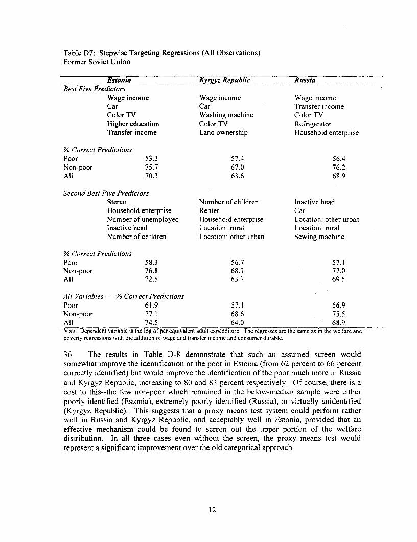
Table D7: Stepwise Targeting Regressions (All Observations)Former Soviet Union

Estonia Kyrgyz Republic RussiaBest Five Predictors _

Wage income Wage income Wage incomeCar Car Transfer incomeColor TV Washing machine Color TVHigher education Color TV RefrigeratorTransfer income Land ownership Household enterprise

% Correct PredictionsPoor 53.3 57.4 56.4Non-poor 75.7 67.0 76.2AIl 70.3 63.6 68.9

Second Best Five PredictorsStereo Number of children Inactive headHousehold enterprise Renter CarNumber of unemployed Household enterprise Location: other urbanInactive head Location: rural Location: ruralNumber of children Location: other urban Sewing machine

% Correct PredictionsPoor 58.3 56.7 57.1Non-poor 76.8 68.1 77.0All 72.5 63.7 69.5

All Variables - % Correct PredictionsPoor 61.9 57.1 56.9Non-poor 77.1 68.6 75.5All 74.5 64.0 68.9Note: Dependent variable is the log of per equivalent adult expenditure. The regresses are the same as in the welfare andpoverty regressions with the addition of wage and transfer income and consumer durable.

36. The results in Table D-8 demonstrate that such an assumed screen wouldsornewhat improve the identification of the poor in Estonia (from 62 percent to 66 percentcorrectly identified) but would improve the identification of the poor much more in Russiaand Kyrgyz Republic, increasing to 80 and 83 percent respectively. Of course, there is acost to this--the few non-poor which remained in the below-median sample were eitherpoorly identified (Estonia), extremely poorly identified (Russia), or virtually unidentified(Kyrgyz Republic). This suggests that a proxy means test system could perform ratherwe]ll in Russia and Kyrgyz Republic, and acceptably well in Estonia, provided that aneffiective mechanism could be found to screen out the upper portion of the welfaredistribution. In all three cases even without the screen, the proxy means test wouldrepresent a significant improvement over the old categorical approach.

12

Table D8: Stepwise Targeting Regressions (Observations Below Median)Former Soviet Union

Estonia Kyrgyz Republic RussiaBest Five Predictors

Wage income Land ownership Wage incomeTransfer income Wage income Color TVColor TV Car Transfer incomeInactive head Motorcycle Education: primaryNumber of unemployed Renter Refrigerator

% Correct PredictionsPoor 64.2 83.0 79.6Non-poor 54.3 0.0 22.4All 63.7 82.0 73.1

Seco1d IBest Five PredcictorsL.and ownership Washing machine' Education: higherLocation: rural Land ownershipL.ducation: voc.-tech Household enterpriseCar ReniterWashing imachine Number of elderly

%o Correct PredctIionsPoor 65.4 83.1 79.6Non-poor 63.1 9.5 22.2All 65.2 81.5 73.0

,4// Vzaritahles - % Correct Predlictionsfloor 65.5 83.1 79.5Non-poor 61.1 8.7 21.8All 65.1 81.3 72.9.'oiL l)ependent variah1c is the log ol'per equivalent aidult expenditure. 'I'he regresses are the same as in the welvfare andpoeCrty regressions wkith the addition of' age and transler income and consumer durable.

O()nl six variablcs mct the: cntr criteriii.

37. Further, in all three countries, the five best predictors alone did as good a job inidentifying the poor (Kyrgyz Republic. Russia) or almost as well (Estonia) as did the fullmodel, implying that only a few key data would be required for collection. As in EasternEurope, the set of predictors which emerges as the best for identifying the poor (given thatthe upper 50 percent of the distribution was screened out of consideration) is more or lessthe same as which resulted from estimation over the full sample. Interestingly enough, forKyrgyz Republic, using the below-median observations resulted in only six variablesmeeting the entry criteria for the forward stepwise regression: land ownership, wageincome, car, motorcycle, renter status, and washing machine. For Russia and Estonia,more than 10 variables entered into the forward stepwise specification.

38. Wage income was still the best indicator in Estonia & Russia, but was displaced tosecond in Kyrgyz Republic by land ownership (which itself was in the top five for the fullsample). In Estonia, ownership of a car and higher education have been replaced by

13

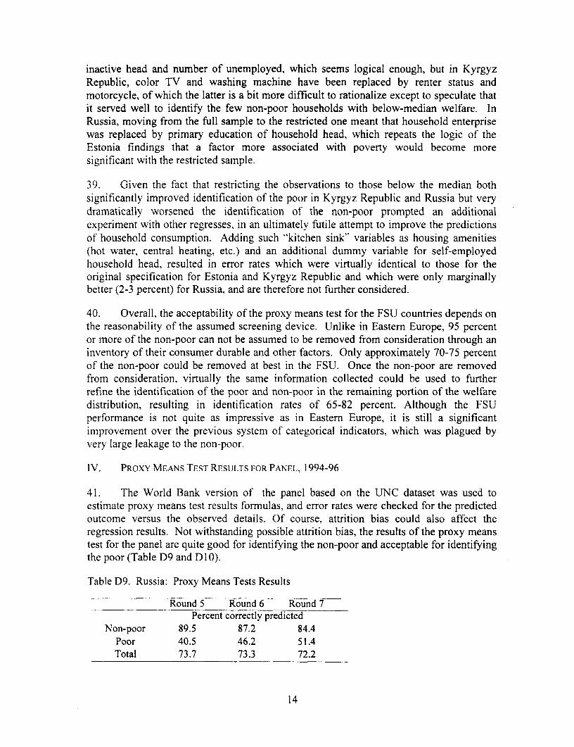
inactive head and number of unemployed, which seems logical enough, but in KyrgyzRepublic, color TV and washing machine have been replaced by renter status andmotorcycle, of which the latter is a bit more difficult to rationalize except to speculate thatit served well to identify the few non-poor households with below-median welfare. InRussia, moving from the full sample to the restricted one meant that household enterprisewas replaced by primary education of household head, which repeats the logic of theEstonia findings that a factor more associated with poverty would become moresignificant with the restricted sample.

39. Given the fact that restricting the observations to those below the median bothsignificantly improved identification of the poor in Kyrgyz Republic and Russia but verydramatically worsened the identification of the non-poor prompted an additionalexperiment with other regresses. in an ultimately futile attempt to improve the predictionsof household consumption. Adding such "kitchen sink" variables as housing amenities(hot water, central heating, etc.) and an additional dummy variable for self-employedhouisehold head, resulted in error rates which were virtually identical to those for theoriginal specification for Estonia and Kyrgyz Republic and which were only marginallybetter (2-3 percent) for Russia, and are therefore not further considered.

40. Overall, the acceptability of the proxy means test for the FSU countries depends onthe reasonability of the assumed screening device. Unlike in Eastern Europe, 95 percentor more of the non-poor can not be assumed to be removed from consideration through aninventory of their consumer durable and other factors. Only approximately 70-75 percentof the non-poor could be removed at best in the FSU. Once the non-poor are removedfrom consideration, virtually the same information collected could be used to furtherrefine the identification of the poor and non-poor in the remaining portion of the welfaredistribution, resulting in identification rates of 65-82 percent. Although the FSUperformance is not quite as impressive as in Eastern Europe, it is still a significantimprovement over the previous system of categorical indicators, which was plagued byvery large leakage to the non-poor.

IV. PROXY MEANS TEST RESUlTJI1S FOR PANEL, 1994-96

41. The World Bank version of the panel based on the UJNC dataset was used toestimate proxy means test results formulas, and error rates were checked for the predictedoutcome versus the observed details. Of course, attrition bias could also affect theregression results. Not withstanding possible attrition bias, the results of the proxy meanstest for the panel are quite good for identifying the non-poor and acceptable for identifyingthe poor (Table D9 and D10).

Table D9. Russia: Proxy Means Tests Results

Round 5 Round 6 Round 7Percent correctly predicted

Non-poor 89.5 87.2 84.4Poor 40.5 46.2 51.4Total 73.7 73.3 72.2

14

IV. CONCLUSIONS

42. This annex has presented four different. sets of proxy means test regressions foridentifying the poor and the non-poor in Russia. First, a model for Russia and Volgogradwas set up and estimated. Second, results from simulations and actual outcomes from thefor World Bank social assistance pilots were compared. Third, simulations for Russiawere compared to two neighboring countries, Estonia and Kyrgyz Republic. Finally, withthese results in mind, proxy mean tests for Russia using our panel (World Bank version ofthe RLMS dataset) were estimated.

15

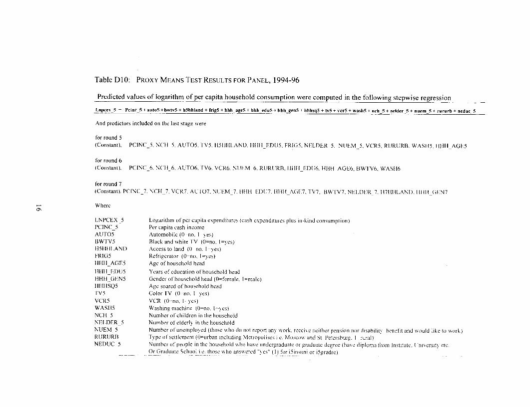
Table D1O: PROXY MEANS TEST RESULTS FOR PANEL, 1994-96

Predicted values of logarithm of per capita household consumption were computed in the following stepwise regression

Lnpcex_5 = Pcinc 5 + auto5 +bwtv5 + h5hhland + frigS + hhh_ageS + hhh_eduS + hhh_gen5 + hhhsq5 + tv5 + vecr5 + wash5 + nch_5 + nelder_5 + nuem 5 + rururb + neduc 5

And predictors included on the last stage w%ere

for round 5(Constant). PCINC_5. NCII 5. AUT05. TV5. 11511111.AND. HHlii EDU5. FRIGS. NE.LDER_5, NJEM_S. VCR5, RURURB. WAS115, l11111 AGE5

for round 6(Constant). PCINC_6. NCII_6. AUT06. TV6. VCR6. NUI-M_6. RURUR13. 1Ill11_ED)U6. IiHH AGE6. 1'WTV6, WAS116

for round 7(Constant). PCINC 7. NCII 7, VCR7 AUTOt7. NJEM_7. IIHI ED[)U7. Hlill_AGF7. TV7. BwrV7 Nl.LDFR 7, 117111.ANI). 111111 (i.N7.

Where

LNPCEX 5 Logarithm of per capita expenditures (cash expenditures plus in-kind consumption)PCINC_5 Per capita cash incomeAUT05 Automobile (Ono. I-,es)BWTV5 Black and white I'V (Ono. I=ves)1151111.ANI) Access to land (0)no. I =ves)FRIG5 Refrigerator (0)no. I=yes)111111_AGE5 Age of household headIIIIII_ID )U5 Years of education of household headIHII_CilGN5 Gender of household head (0=female. I =male)IIIIIISQ5 Age soared of household headIV5 Color'l V (0 -no. I-yes)VCR5 VCR (0-(no. I yes)WASH5 Washing machiie (0=no, I=vcs)NCH S Number of children in the householdNELDER 5 Number of elderly in the householdNUEM_5 Number of unemployed (those wN ho do not report any work. receis e neither pension nor disability henefit and would like to work)RURURB type of'settlement (O=urban incIliding Metropolises i.e. Moscom and St. Petersburg. I =rural)NEDUC_5 Nurnber of people in thc household %sho have undergraduate or graduLate degree (have diploma from Institute. U niversity etc

Or Graduate School i.e. those who answsered "yes" (I) for i5insuni or i5gradre)

ANNEX FIVE

Tide Welfare Mobility, Poverty and Inequality in Russia In 1994-1"996 -

Authors Elena GlinskayaCarolina Population Center, University of North Carolina at Chapel HillJeanine BraithwaitoWorld Bank

O)bjectives Examine households' one- and two- year trnsitions between quintiles of =comc andiexpenditure distributions.

Investigate relationship between changes in position within distributionsof xfeitarandicharacteristics of households.

Data Three waves (1994, 1995, 1996) of the Russia Longitudinal Monitoring Survey (RLMS)

Empirical model

,* - P,,, = 30j + 03

4,j ' + 2q/ X1,,, + P33. X2 is,j ,4qj li,- e

for P=1.2.3,4.5

-*w,ere:I, indicates initial quintile of distribution, at time to. j= {l..5)p.. indicate percentile in thc welfare distribution at time t.p,1., indicate percentile in the welfare distribution at time r-/,I binasy indicator. tak-es value i' 1" for the observation fiom 1995-1996, and 'O" for; t!94-1995:

XI,, vectc' of characteristics of the household head:a: and age squared of the household bcad,education and cducation squared of the household head,occupation of the household head,St .:der of the household head;

X2,, vectoi of characteristics of demographic composition of the household and indicators of presence ofhousehold members from specific groups:

IF rPportion of chiTdren aged I months 6 years in the household,pFsportion of cihildren aged 7 years - 17 years in the household,pr, portion of active females (18-60 years old) in the household,propbortion of retircd males (61+ years old) in the household,preportion of retired females (55+ years old) in the household,houschold sizc

in' iicator for presence of handicaped persons in the householdindicator for presence of persons on maternity leave in the households

ZL, vector cif indicators:eight regions of the Russian Federationrural

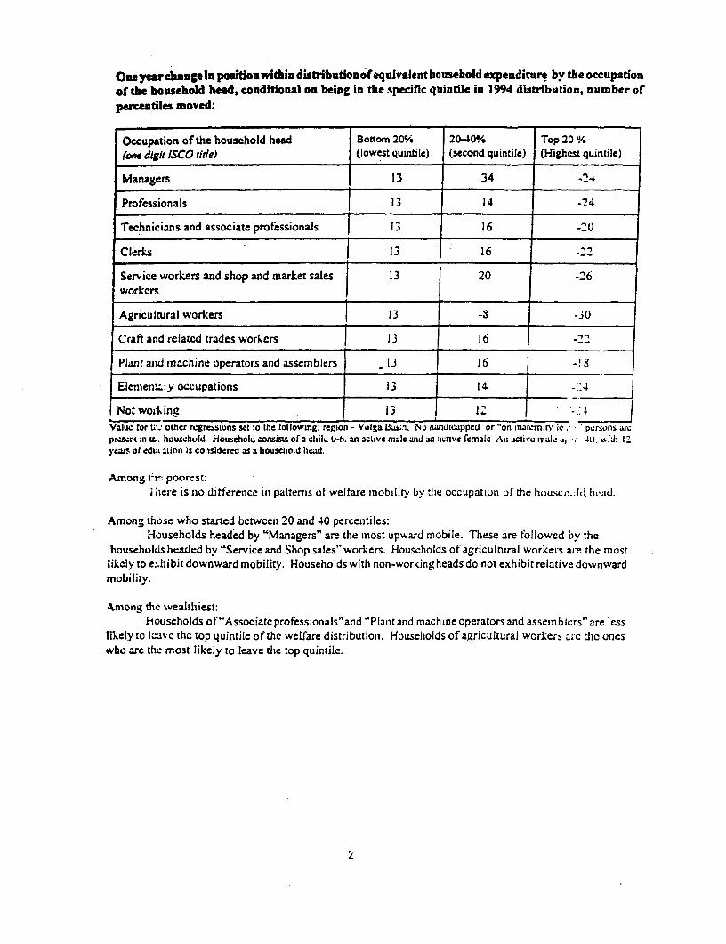
Oneyearcnge lo positionwithin distribution ofequivalent household expenditure by the occupationof the bhusehold head, conditional oan being in the specfic quintile in 1394 distribution, number ofpercentiles moved:

Occupation of the household head Bottom 20W 20-40% Top 20 %(one digit ISCO title) (lowest quintile) (second quintile) (Highest quintile)

Managers 13 34 _

Profcssionals 14 -24

Technicians and associate professionals 13 16 -20

Clerls 13 16 -22

Service workers and shop and mark-et sales 13 20 -26workcrs

Agricultural work-ers 13 3 -30

Craft and related trades workers 13 16

Pl ant and machine operators and assemblers 13 16 - 8

Elmenlen:y occupations 13 14

I Not working f 13 j 1 .Valuc for tL oher regressions sei 1he following: re-ion - Vulga Basm. No ?iandicapped or 'on Inacemirv ic ' persons auxpresent in tL.. houschuld. klouschold consists of a chlild 0-h. an active male and au urive female Aun active Uaho al ;e i. u,idi 12years of cduL ion is considered as a bouschold hlcad.

Among 1ic: poorcst:-There is no ditfference in patterns ofwelfare mobility bv tie occupation of the lhuuscnl_k4 hclid.

Among those who started bctwcezi 20 and 40 percentiles:Households headed by 'Managers" are the most upward mobile. These are followcd by the

households headed by "Service and Shop sales" work-ers. Households of agricultural workers are the mostlikcly to e.:hibit downward mobility. Households with non-working heads do not exhibit relative dowvnwardmobility.

4nmong the wealthiest:Houscholds of"Associatc professionals"and "Plant and machine operators and assembibers" are less

likely to Icavc thc top quintile of thc welfare distribution. Households of agricultural workers aic die oneswho are the most likely to leave the top quintile.

2

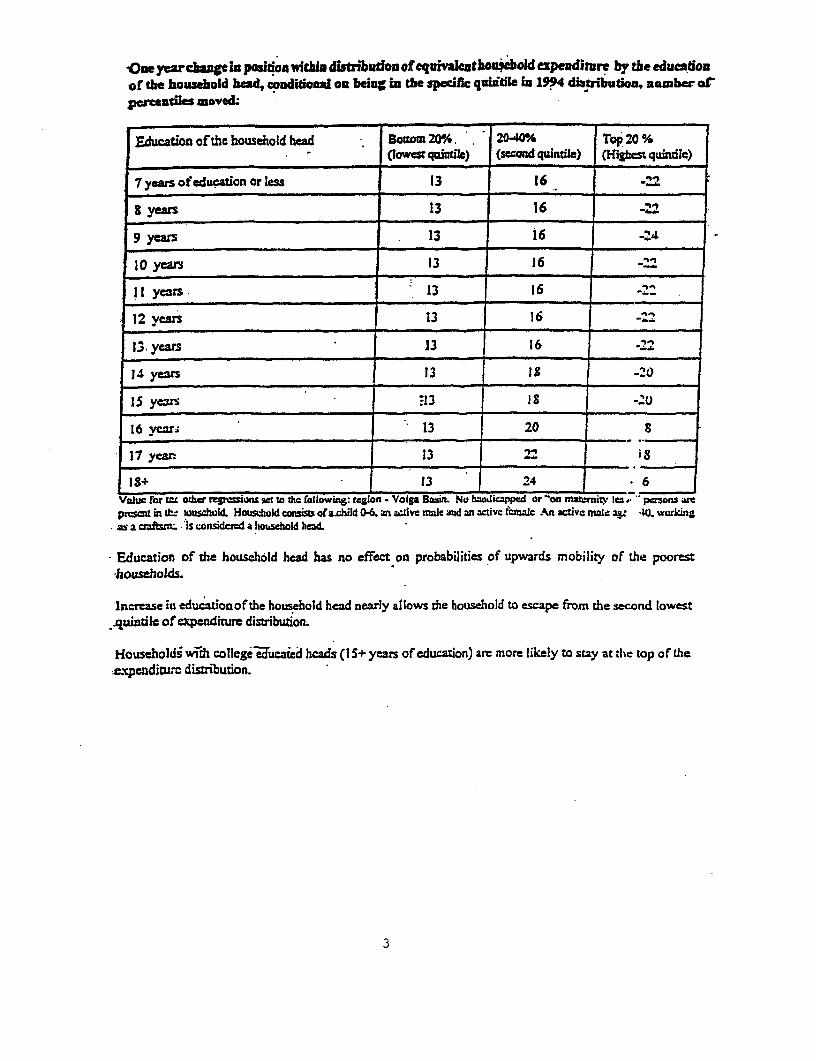
Otae yeardagtei positiOn witCl distribution of equivavth*oubold expenditure by the educs.tionof the household bhed, conditioal on being in the specific quitile In 1994 distribution, number ofercenties moved.

Education of the household head Boam 20A. 2040% Top 20 %(lowest quimile) (second qwnnle) (Higcst quindle)

7 years of education or less 13 16 6

8 years 13 16 -

9 year-s ~~~~~13 16 -24

10 ye= ~~~~~~13 16-2

3 6 . _ 1

12 yas 13 16 -22

13. years 13 16 -_

14 yeas 3 6 -20

5ye=.13 -'l

16 year.; 13 _ 1

I year. 13 22 1

+ _.24Value for W= OUter regmaions sel to hc following: tcgion - Volpa Basin. No hwidic.Vppd or 'on matomity lea .. Paso" amc

psctin Utl- iunscwod. Housnctold consists ota.child 0.6. an aaive male saud anf =cive tci?iac AA active maLn anj -40. %varking_a a aaf.s. .is ctnsidemd a ..ouschold hod.

F-ducation of the houselhold head has no effect on probabilities of upwards mobility of the poorest,households.

lncrease in educ~ationof the household head nearly allows the household to escape fromr the second lowest.quizftile of expenditue distribution.

Hiouscboldi wtid college'-ucaica heads (15+ years of education) are more likely to stay at thic top of the&xpendiruzc distribution.

3

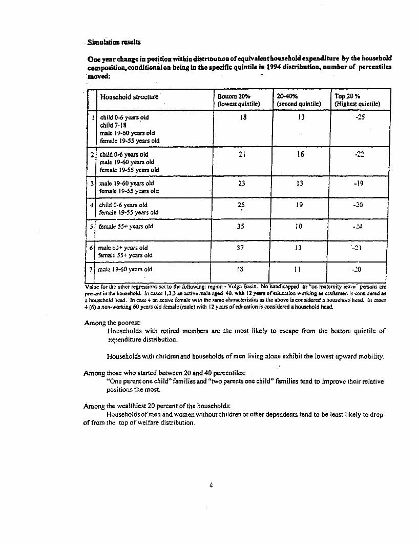
Simui on msuIts

One year change in position within distrioution of eq uivalent household expenditure by the householdcomposition,conditionalon being in the specific quintile in 1994 distribution, number of percentiles*moved:.

Household structure Bottom 20% 20W400 Top 20 %(lowest quintile) (second quintile) (Highast quintile)

I child 0-6 years old 18 13 -25child 7-18male 19-60 years oldfemale 19-55 years old

2 cbild 0-6 years old 21 16 on-male 19-60 years oldfemale 19-55 years old

3 male 19-60 years old 23 13 -19female 19-55 years old

4 child 0-6 years old 25 19 -20female 19-55 years old

if fem i55+ years old 35 10 -24

6 male 60+ years old 37 13female 55+ years old

7i male 1 -60 years old 18 I1 -20

Value for the other regressions set to the following. region - Volga Basin. No handicapped or 'on matcmity Ica-mc persons arepresent in the household. In cascs 1,2.3 an active male nged 40. with 12 years of education working as craftsmeo is wonsidered asa household hcad. In case 4 an active female with the saene characteristics as the above is considered a household head. In cases4 (6) a non-wvorking 60 ycars old female (male) with 12 years of education is considered a household head.

Among the poorest:Households with retired members arc thc most likefy to escape from the bottom quintile ofexpenditure distributioti.

'Households with children and households of men living alone exhibit the lowest upward mobility.

Among those who started between 20 and 40 percentiles:'One parent one child" families and "two parents one child" families tend to improvc their relativepositions the most.

Among the wcalthiest 20 percent of the households:Households of men and women withoutcchildren or other dependents tend to be least likely to drop

of from the top of welfare distribution.

4

Estimation method OLS with cluster correction for the household spesific autogregressive errors

Findings

There is substantial mobility within the distributions of household income and expenditurcs.Between 1994 and 1995, the probability of staying in the lowest quintile of the per-capita expendituredistribution was 0.46, and between 1994 and 1996 (the two year probability) it was 0.39. Persistence ofremaining in the top quintile of the per capita distributionsis higher than the persistence of remaining in thelowest quintile.

a Accounting for mobility within the distributions of the housceiolds' welfare decreasei measurmdinequality.

- The pattem of mobility between quintiles of income distributions is similar to the patzern ofnobility between quintilesof cxpendituredistributions. This might indicate that households find it diftcultto smooth their current consumption following fluctuations in current income.

* Demographic composition of the household is a significant determinant of degree and directionof mobility at all points of the initial welfare distribution.

* Occupation of the household head is a significant dcterminant of the households proh-ability ofmaovin" fiv the households in the central and higih percentiles (i.e. all, except bottom 20 perce-viles) ot theinitial weitire distribution.

* Y. .rs of education of the houschold head are positively related to upward moveineiitb ni theincome an; expenditure ladders for the households from higher (top 40) percentilesof the initial ,;istribution.

* Th^re are no significant ditferences in the extent and direction of mobility by the age f thehousehold head. Among households in dte central part of the initial distribution (40-80 percentiles) femaleheaded households show higher upward mobility than male headed households. There is no e6idence thatpatterns of households'welfare mobility differ by the presence of handicapped members and members onmaternity lcave.

* Patterns of households' welfare mobility are significantly different among the regions of theRussian Federation. At all points of the initial distribution. households residing in the metrovolitan iteas,Moscow and St. Peterburg) tend to irnprove their reiative positions. i nese is some evide,nce that ruralrcsidt:t.s are *nore likely to exhibit downward mobillity.

5

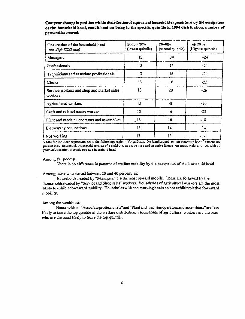
Oneyearchangeh positionwithindistnrbutionof equivalent householdexpenditure by the occupationof the household head, conditional on being in the specific quintUle in 1994 distribution, number ofpercentiles moved:

Occupation of the household head Bottom 20°/e 2040% Top 20 %(one digit ISCO title) (lowest quittile) (second quintile) (Highcst quintile)

Managers 13 34 4

Professionals 13 14 -24

Technicians and associate professionals 13 16 -20

Clerkus 1;3 16

Service work-ers and shop and market sales 13 20 -26workcrs

Agricultural workers 13 -8 -30

Craft and related trades workers 1 3 1

Plant and machine operators and assemblers .13 16 18

Elemen= :y occupations 13 14

Not workLing 13 12Value for tW other regressions set to the following: region - Vulga Baia6n. No handicapped or 'on macemi le .- persons armpris.2nt in tr.. household. Household consists of a child 0-. an active niale and ani active female Ani activc male a1 41). %vith 12years of edL;L aion is conisidered as a household hcad.

Among t-n; poorcst:Th1ere is no difference in patterns of welfare mobility by thie occupation of the houscti.d. hcad.

Among those who started bctwcen 20 and 40 percentiles:Households headed by "Managers" are the most upward mobile. These are followed by the

houselioldsheaded by "Serviceand Shop sales"workers. Households of agricultural workers are the mostlikely to e~.hibit downward mobility. Households with non-working heads do not exhibit relative dowvnwardmobiliry.

Among the wealthiest:Households of `Associate professionals"and "Plant and machine operators and assem biers" are less

likely to icavc thc top quintile of thc welfare distribution. Households of agricultural work-ers a;c the oneswho are the most likely to leave the top quintile.

6