relationships between statistics of rainfall extremes and mean

Hydrol. Earth Syst. Sci., 10, 589–601, 2006www.hydrol-earth-syst-sci.net/10/589/2006/© Author(s) 2006. This work is licensedunder a Creative Commons License.

Hydrology andEarth System

Sciences

Relationships between statistics of rainfall extremes and meanannual precipitation: an application for design-storm estimation innorthern central Italy

G. Di Baldassarre, A. Castellarin, and A. Brath

DISTART, Faculty of Civil Engineering, University of Bologna, Bologna, Italy

Received: 16 September 2005 – Published in Hydrol. Earth Syst. Sci. Discuss.: 16 November 2005Revised: 19 April 2006 – Accepted: 26 July 2006 – Published: 21 August 2006

Abstract. Several hydrological analyses need to be foundedon a reliable estimate of the design storm, which is the ex-pected rainfall depth corresponding to a given duration andprobability of occurrence, usually expressed in terms of re-turn period. The annual series of precipitation maxima forstorm duration ranging from 15 min to 1 day, observed at adense network of raingauges sited in northern central Italy,are analyzed using an approach based on L-moments. Theanalysis investigates the statistical properties of rainfall ex-tremes and detects significant relationships between theseproperties and the mean annual precipitation (MAP). On thebasis of these relationships, we developed a regional modelfor estimating the rainfall depth for a given storm durationand recurrence interval in any location of the study region.The applicability of the regional model was assessed throughMonte Carlo simulations. The uncertainty of the model forungauged sites was quantified through an extensive cross-validation.

1 Introduction

Design storm are usually estimated by regional frequencyanalysis of rainfall extremes when there are no measured datafor the location of interest, or when data record lengths areshort compared to the recurrence interval of interest (Brathet al., 1998; Faulkner, 1999; Brath and Castellarin, 2001).

This study analyses the annual series of precipitation max-ima observed at a dense raingauge network located in a widegeographical area of northern central Italy. Several regionalfrequency analyses of rainfall extremes were performed overthe study area analysed here in (Franchini and Galeati, 1994;Brath et al, 1998). These studies proposed subdivisions ofthe region into homogeneous climatic regions, within which

Correspondence to:G. Di Baldassarre([email protected])

the statistics of rainfall extremes for a given duration are as-sumed to be constant (Brath and Castellarin, 2001). This as-sumption contrasts with the findings of other studies, whichshow that the statistics of rainfall extremes vary systemati-cally with location (Schaefer, 1990; Alila, 1999; Brath et al.,2003). These studies also identified statistically significantrelationships between these statistics and the mean annualprecipitation (MAP), which was used as a surrogate of geo-graphical location.

For instance, Schaefer (1990) analysed the rainfall se-ries collected at hundreds of gauges located in WashingtonState (USA) and showed that the coefficients of variation andskewness of rainfall extremes tend to decrease as the localvalue of MAP increases. Alila (1999) studied the Canadianraingauge network and detected analogous relationship be-tween the L-coefficients of variation, L-Cv (for a definitionof the coefficients see e.g. Hosking and Wallis, 1997). Brathet al. (2003) identified a similar behaviour of L-Cv and L-Cs(L-coefficients of skewness) of rainfall extremes for the samestudy area considered herein and storm-duration between 1and 24 h. We investigated further the applicability of theseoutcomes to the study region for sub-hourly storm-durationand, on the basis of the findings obtained, we formalisedthe relationship between L-statistics of rainfall extremes andMAP through a Horton-type curve (Horton, 1939). Once as-sessed the applicability of the proposed mathematical expres-sion through an original and objective Monte Carlo simula-tion experiment, we developed a regional model for estimat-ing design storms for storm duration from 15 min to 1 dayin any location of the study area and we quantified the un-certainty of the regional model for ungauged sites through anextensive cross-validation.

Published by Copernicus GmbH on behalf of the European Geosciences Union.

590 G. Di Baldassarre et al.: Regional model for design storm estimation

2 Index storm procedure

The design of numerous hydraulic engineering structures andseveral hydrological applications need to be based on an es-timate of a design storm, which is the expected rainfall depthh(d,T ) corresponding to a given durationd and probabilityof occurrence, usually expressed in terms of return periodT .

A regional frequency analysis can be implemented usingthe index storm procedure (Dalrymple, 1960; Brath et al.,2003). The index storm methodology is based on the iden-tification of homogeneous groups of sites for whichh(d,T )

can be expressed as the product of two terms, as follows:

h(d, T ) = mdh′(d, T ) (1)

these two terms are a scale factormd , which is called indexstorm, and a dimensionless growth factorh′(d,T ), which de-scribes the relationship between the dimensionless storm andthe recurrence interval. The index storm, usually assumedequal to the mean of annual rainfall maxima of durationd,is site dependent; while the growth factor is assumed to bevalid for the entire homogeneous group of basins.

2.1 Growth factor estimation

The classical implementation of the index flood procedure(or index storm if reference is made to rainfall extremes)is based on the most restrictive fundamental hypothesis ofexistence of homogeneous regions within which the statis-tical properties of dimensionless rainfall extremes (see e.g.,Franchini and Galeati, 1994; Brath et al., 1998) do not varywith location (i.e., coefficients of variation and skewness, orequivalently L-Cv and L-Cs, are constant).

Nevertheless, since the original procedure was introduced(see e.g. Dalrymple, 1960) several extensions and evolutionswere proposed, which partly relax this fundamental hypoth-esis. An example is the hierarchical application of the indexflood hypothesis, where the statistics of increasing order areconstant within a set of nested regions, the larger the orderof the statistics, the larger the region (see e.g. Gabriele andArnell, 1991). Another relevant example of evolution of theoriginal hypothesis is the Region of Influence approach (e.g.,Burn, 1990; Castellarin et al., 2001), which adopts the con-cept of homogeneous pooling groups of sites as opposed tohomogeneous geographical regions. We present a regionalmodel that can be considered to be an extension of the indexflood model as well. Similarly to what originally proposedin Schaefer (1990) and Alila (1999), we assume that a homo-geneous region, within which L-Cvand L-Csare constant, isa group of climatically homogeneous sites, within which thevariability of MAP is very limited.

The study described in this paper investigates the applica-bility of the findings of Schaefer (1990) and Alila (1999) in alarge geographical area of northern central Italy. The analy-sis considers annual series of precipitation maxima for storm

duration from 15 min to 1 day that were observed by a denseraingauge network.

We characterised the regional frequency regime of rain-fall extremes over the study area using the L-moments assuggested by Hosking and Wallis (1997). The L-momentsare analogous to the conventional moments, but they havethe theoretical advantages of being able to characterize awider range of distributions and, when estimated from a sam-ple, of being more robust to the presence of outliers in thedata. Hosking and Wallis (e.g., 1997) also point out that L-moments are less subject to bias in estimation than conven-tional moments. Nevertheless, Klemes (2000) considered thelack of sensitivity to outliers to be a disadvantage in the useof L-moments. The recent study (Klemes, 2000) argues thathigh outliers in a hydrologic data series are important for ex-trapolating to large return period events as they control theright tail of the frequency distribution.

The growth factor estimation was performed by using theGeneralised Extreme Value (GEV) distribution (Jenkinson,1955). The GEV distribution subsumes all three differentextreme-value distributions (i.e., EV type I, II and III), towhich the largest/smallest value from a set of independentand identically distributed random variables asymptoticallytends. Consistently, several recent regional analyses showedthat the GEV distribution is a suitable statistical model forrepresenting the frequency regime of rainfall extremes overthe whole study area (see e.g., Franchini and Galeati 1994;Brath et al. 1998).

The CDF (cumulative distribution function) of the GEVdistribution is written as:

FX(x) = exp

{−

[1 −

k(x − ξ)

α

]1/k}

, for k 6= 0 (2a)

and

FX(x) = exp

{− exp

[−

(x − ξ)

α

]}, for k = 0 (2b)

while the quantilex(F ) can be written as:

x(F ) = ξ + α{1 − (− logF)k

}/k, for k 6= 0 (3a)

and

x(F ) = ξ + α log(− logF), for k = 0 (3b)

whereξ , α, andk are the distribution parameters. As shownby Eqs. (2b) and (3b), whenk=0 the GEV distribution isequal to the Gumbel distribution. Combining formulations(2) and (3) can be obtained the relations for the regionalgrowth factor, replacing the variableX with the dimension-less variableX’=X/µ and the parametersα, ξ andkwith theregional parametersα′=α/µ, ξ ’=ξ /µ andk′=k, where the ex-pected valueµ is written as:

µ = ξ +

(α

k

)[1 − (1 + k)] . (4)

Hydrol. Earth Syst. Sci., 10, 589–601, 2006 www.hydrol-earth-syst-sci.net/10/589/2006/

G. Di Baldassarre et al.: Regional model for design storm estimation 591

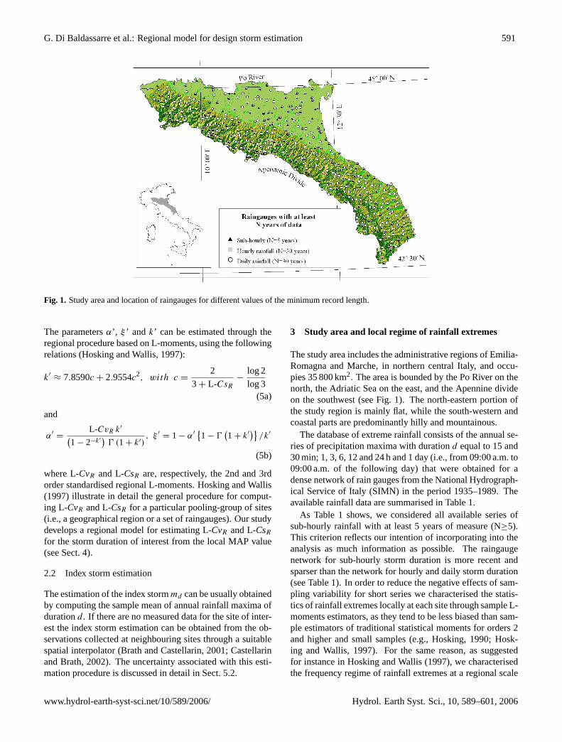
Fig. 1. Study area and location of raingauges for different values of the minimum record length.

The parametersα’, ξ ’ and k’ can be estimated through theregional procedure based on L-moments, using the followingrelations (Hosking and Wallis, 1997):

k′≈ 7.8590c + 2.9554c2, with c =

2

3 + L-CsR−

log 2

log 3(5a)

and

α′=

L-CvR k′(1 − 2−k′

)0 (1 + k′)

, ξ ′= 1 − α′

{1 − 0

(1 + k′

)}/k′

(5b)

where L-CvR and L-CsR are, respectively, the 2nd and 3rdorder standardised regional L-moments. Hosking and Wallis(1997) illustrate in detail the general procedure for comput-ing L-CvR and L-CsR for a particular pooling-group of sites(i.e., a geographical region or a set of raingauges). Our studydevelops a regional model for estimating L-CvR and L-CsRfor the storm duration of interest from the local MAP value(see Sect. 4).

2.2 Index storm estimation

The estimation of the index stormmd can be usually obtainedby computing the sample mean of annual rainfall maxima ofdurationd. If there are no measured data for the site of inter-est the index storm estimation can be obtained from the ob-servations collected at neighbouring sites through a suitablespatial interpolator (Brath and Castellarin, 2001; Castellarinand Brath, 2002). The uncertainty associated with this esti-mation procedure is discussed in detail in Sect. 5.2.

3 Study area and local regime of rainfall extremes

The study area includes the administrative regions of Emilia-Romagna and Marche, in northern central Italy, and occu-pies 35 800 km2. The area is bounded by the Po River on thenorth, the Adriatic Sea on the east, and the Apennine divideon the southwest (see Fig. 1). The north-eastern portion ofthe study region is mainly flat, while the south-western andcoastal parts are predominantly hilly and mountainous.

The database of extreme rainfall consists of the annual se-ries of precipitation maxima with durationd equal to 15 and30 min; 1, 3, 6, 12 and 24 h and 1 day (i.e., from 09:00 a.m. to09:00 a.m. of the following day) that were obtained for adense network of rain gauges from the National Hydrograph-ical Service of Italy (SIMN) in the period 1935–1989. Theavailable rainfall data are summarised in Table 1.

As Table 1 shows, we considered all available series ofsub-hourly rainfall with at least 5 years of measure (N≥5).This criterion reflects our intention of incorporating into theanalysis as much information as possible. The raingaugenetwork for sub-hourly storm duration is more recent andsparser than the network for hourly and daily storm duration(see Table 1). In order to reduce the negative effects of sam-pling variability for short series we characterised the statis-tics of rainfall extremes locally at each site through sample L-moments estimators, as they tend to be less biased than sam-ple estimators of traditional statistical moments for orders 2and higher and small samples (e.g., Hosking, 1990; Hosk-ing and Wallis, 1997). For the same reason, as suggestedfor instance in Hosking and Wallis (1997), we characterisedthe frequency regime of rainfall extremes at a regional scale

www.hydrol-earth-syst-sci.net/10/589/2006/ Hydrol. Earth Syst. Sci., 10, 589–601, 2006


Table 1. Study Area: Number of Raingauges and Annual Maximum Rainfall Data.

Duration Criterion Number of Gauges Station-year of data

daily N≥30 394 20557hourly N≥30 125 594530 min N≥5 186 343015 min N≥5 152 1810

Fig. 2. Mean annual precipitation MAP (mm). MAP versus Altitude (m a.s.l.).

(i.e., for a group of raingauges) by weighting each sampleL-moment proportionally to the sample length.

A regional analysis of the dates of occurrence of short-duration rainfall extremes (i.e., 1 or 3 h) pointed out signif-icant consistency and a mean timing which varied betweenthe end of July and the beginning of August for the entirestudy area (Castellarin and Brath, 2002). This is consistentwith the observation that in the study area the hourly rainfallextremes are almost invariantly summer showers generatedby local convective cells. The dates of occurrence of long-duration rainfall extremes (i.e., 24 h or 1 day) showed lessregularity and a mean timing that ranges between the begin-ning of September and the beginning of November.

MAP varies on the study region from about 500 to2500 mm. Altitude is the factor that most affects the MAP(see Figs. 1 and 2), which exceeds 1500 mm starting fromaltitudes higher than 400 m a.s.l. and exhibits the highestvalues along the divide of the Apennines.

The diagram of L-moment ratios (see e.g., Hosking andWallis, 1993) reported in Fig. 3 shows that the theoretical re-

lationship between L-skewness (L-Cs) and L-kurtosis (L-Ck)for the GEV distribution is very close to the regional L-Csand L-Ck values for all storm duration of interest, thereforeindicating that the GEV distribution is a suitable parent dis-tribution.

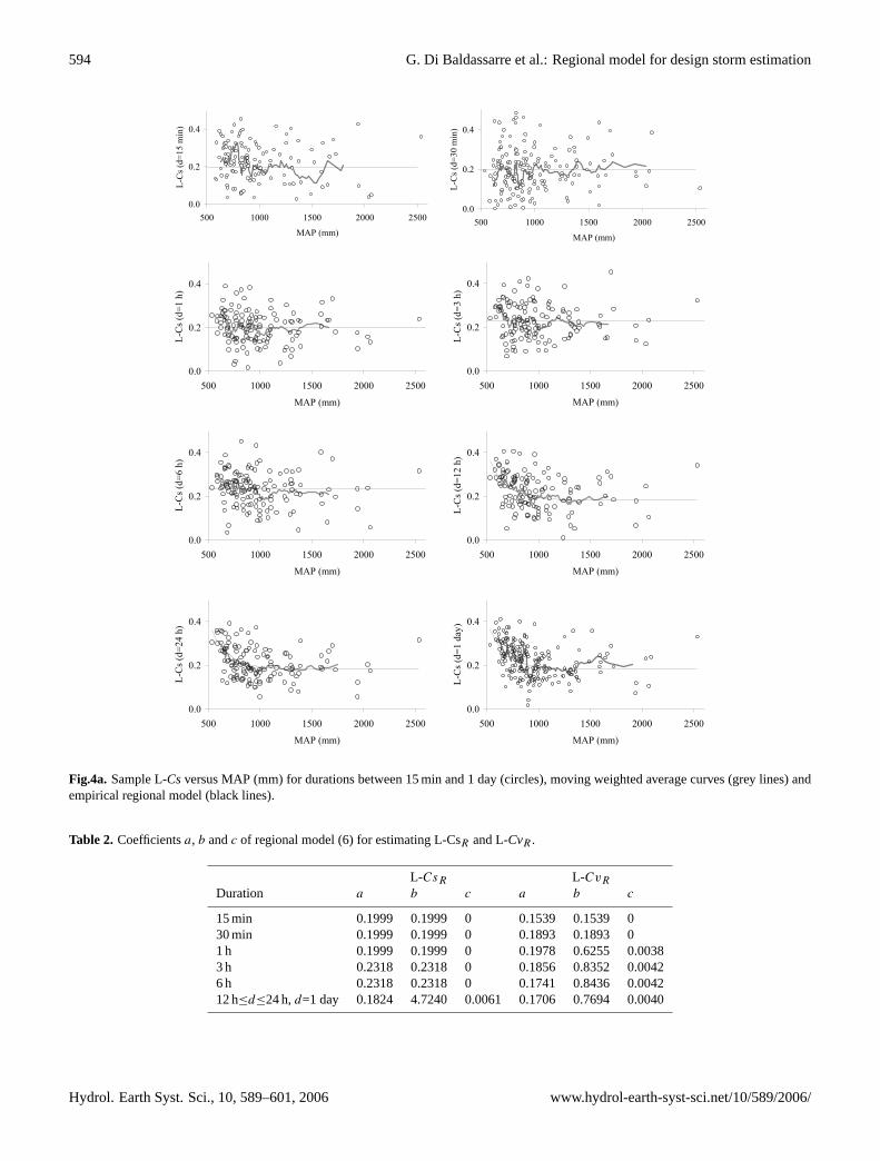
The study investigates the applicability of the finding ofSchaefer (1990) and Alila (1999) in this particular context,making use of a raingauge network with a higher resolu-tion than the networks considered in the above mentionedpapers. The variability of the sample L-moment ratio (Hosk-ing, 1990) of skewness and variation was examined againstthe variability of MAP. Figure 4 shows that the values of L-Cv and L-Cs of rainfall extremes tend to increase when theMAP value decreases, confirming some of the results pointedout by Alila (1999).



4 Regional model

4.1 Climatically homogeneous pooling-groups

As previously mentioned, the estimation of the dimension-less growth factorh′(d,T ) can also be carried out by dis-pensing with the traditional subdivision of the study area intohomogeneous regions. In fact, the papers of Schaefer (1990)and Alila (1999) point out that the statistics of rainfall ex-tremes vary systematically with location, showing that all hy-potheses of subdivisions into geographical regions lack phys-ical basis. These studies identified statistically significant re-lationships between these statistics and the MAP, which wasused as a surrogate of geographical location.

We developed frequency analysis of rainfall extremes us-ing the MAP values and the L-moments L-Cs and L-Cv(Hosking and Wallis, 1997), for any considered duration (d

equal to 15 and 30 min; 1, 3, 6, 12 and 24 h; 1 day). The anal-ysis points out that the L-Cv values tend to decrease as thelocal value of MAP increases (see Fig. 4); for storm durationfrom 15 min to 6 h the L-Cs values are approximately con-stant with the geographic position (identified with the MAPvalue); for longer storm duration the L-Csvalues tend to de-crease as the local value of MAP increases.

We designed and performed a statistical homogeneity testwhich uses the heterogeneity measures proposed by Hosk-ing and Wallis (1993) but also incorporates the findings ofSchaefer (1990) and Alila (1999) by grouping the stationsthat show similar MAP values. The statistical test (see alsoAppendix) assesses the homogeneity of a group of stationsaccording to 2 measures of dispersion of the sample L-moments:

1. H(1), that focuses on the dispersion of sample L-Cvval-ues;

2. H(2), that focuses on the combined dispersion of sampleL-Cv and L-Csvalues.

Hosking and Wallis (1993) suggested that the region or groupof sites should be considered as acceptably homogeneous ifH<1; possibly heterogeneous if 1≤H<2, and definitely het-erogeneous if H≥2.

The homogeneity testing has been developed in the follow-ing steps: the set of N raingauges was sorted in ascending or-der of MAP values; with this ordered set, theN−n+1 subsetswere identified considering, each time, then closer station interms of MAP (withn=15, 30, 60); the H(1) values were cal-culated for each group of 15 and 30 stations, while the H(2)values were calculated for the groups with 30 and 60 stations.The H(1) and H(2) values were assigned to the average MAPvalue of the subset and the behaviour of H(1) and H(2) valuesas a function of MAP was then analysed. The different num-bers of raingauges considered for the homogeneity testing(i.e., 15 and 30 for H(1) and 30 and 60 for H(2)) reflect twodifferent aspects. First, higher order L-moments tend to be

1 hr

3 hr

6 hr12 hr

24 hr

0.10

0.15

0.20

0.15 0.20 0.25L-Cs

L-C

k

GumbelGeneralized Extreme ValueGeneralized ParetoGeneralized LogisticRegional sample L moments

Fig. 3. Diagram of L-moment ratios for the application data.

more homogeneous in space than the lower order ones (seee.g., Hosking and Wallis, 1997), therefore pooling-groups ofsites for which the homogeneity is assessed in terms of L-Cvand L-Cs(i.e., use of H(2)) may be lager than pooling-groupsfor which the homogeneity is assessed in terms of L-Cvonly(i.e., use of H(1)). Second, heterogeneity measures such asH(1) and H(2) are better at indicating heterogeneity in largeregions, while have a tendency to give false indications of ho-mogeneity for small regions, therefore pooling groups shouldbe as larger as possible. This analysis (see Fig. 5) shows thatthe subsets identified according to the MAP value are gen-erally acceptably homogeneous, whereas the H(1) value forthe whole study region is equal to 3.41 while the H(2) valueis equal to 1.73. Also, Fig. 5 shows that the H(1) and H(2)values, quantifying the homogeneity degree, are significantlyMAP independent. This result underlines the advantage ofusing MAP a surrogate of geographical location.

4.2 Empirical regional model for estimating the L-Cv andL-Cs

After testing the regional homogeneity of the climaticallysimilar group of sites (identified according to MAP val-ues) the analysis has been directed to develop an empiricalregional model for estimating the regional statistics L-CsRand L-CvR, which can then be used for estimating the GEVparameters.

In detail, we formalised the relationships between L-moments and MAP illustrated in Fig. 4 using a Horton-typecurve::

L−Cx(MAP) = a + (b − a) × exp(−c × MAP), (6)



0.0

0.2

0.4

500 1000 1500 2000 2500

MAP (mm)

L-C

s (d=

15 m

in)

0.0

0.2

0.4

500 1000 1500 2000 2500

MAP (mm)

L-C

s (d=

30 m

in)

0.0

0.2

0.4

500 1000 1500 2000 2500

MAP (mm)

L-C

s (d=

1 h)

0.0

0.2

0.4

500 1000 1500 2000 2500

MAP (mm)

L-C

s (d=

3 h)

0.0

0.2

0.4

500 1000 1500 2000 2500

MAP (mm)

L-C

s (d=

6 h)

0.0

0.2

0.4

500 1000 1500 2000 2500

MAP (mm)

L-C

s (d=

12 h

)

0.0

0.2

0.4

500 1000 1500 2000 2500

MAP (mm)

L-C

s (d=

24 h

)

0.0

0.2

0.4

500 1000 1500 2000 2500

MAP (mm)

L-C

s (d=

1 da

y)

Fig.4a. Sample L-Csversus MAP (mm) for durations between 15 min and 1 day (circles), moving weighted average curves (grey lines) andempirical regional model (black lines).

Table 2. Coefficientsa, b andc of regional model (6) for estimating L-CsR and L-CvR .

L-CsR L-CvR

Duration a b c a b c

15 min 0.1999 0.1999 0 0.1539 0.1539 030 min 0.1999 0.1999 0 0.1893 0.1893 01 h 0.1999 0.1999 0 0.1978 0.6255 0.00383 h 0.2318 0.2318 0 0.1856 0.8352 0.00426 h 0.2318 0.2318 0 0.1741 0.8436 0.004212 h≤d≤24 h,d=1 day 0.1824 4.7240 0.0061 0.1706 0.7694 0.0040



0.0

0.2

0.4

500 1000 1500 2000 2500

MAP (mm)

L-C

v (d

=15

min

)0.0

0.2

0.4

500 1000 1500 2000 2500

MAP (mm)

L-C

v (d

=30

min

)

0.1

0.2

0.3

500 1000 1500 2000 2500

MAP (mm)

L-C

v (d

=1 h

)

0.1

0.2

0.3

500 1000 1500 2000 2500

MAP (mm)

L-C

v (d

=3 h

)

0.1

0.2

0.3

500 1000 1500 2000 2500

MAP (mm)

L-C

v (d

=6 h

)

0.1

0.2

0.3

500 1000 1500 2000 2500

MAP (mm)

L-C

v (d

=12

h)

0.1

0.2

0.3

500 1000 1500 2000 2500

MAP (mm)

L-C

v (d

=24

h)

0.1

0.2

0.3

500 1000 1500 2000 2500

MAP (mm)

L-C

v (d

=1 d

ay)

Fig. 4b. Sample L-Cvversus MAP (mm) for durations between 15 min and 1 day (circles), moving weighted average curves (grey lines) andempirical regional model (black lines).

where L-Cx represents a particular regional L-moment (L-CsR or L-CvR), related to the annual maximum series (AMS)of rainfall depth with storm durationd, while a, b, c, with0≤a≤b andc≥0, are the parameters of the empirical modelthat have to be estimated through an optimisation procedure.If a = b andc=0, Eq. (6) has a constant value. This is thecase in which the particular L-moment is MAP independent.

We performed the identification of parametersa, b andc

on the basis of the empirical outcomes illustrated in Fig. 4,also taking into account the conclusions of previous studiesperformed over the same study region (e.g., Franchini andGaleati, 1994; Brath and Franchini, 1999; Castellarin andBrath, 2002), which can be sketched as follows:

1. L-Cs can be considered to be independent of the geo-graphic location (or MAP) for d<6 h;

2. L-Cscan be considered to be independent of geographiclocation and durationd, for d=15 and 30 min and 1 h;

3. L-Cscan be considered to be the same for duration d=3and 6 h (Castellarin and Brath, 2002);

4. L-Cv can be considered to be independent of the ge-ographic location (or MAP) for d<1 h, with differentvalues for d=15 and 30 min ;

5. The relationships between L-Cs, or L-Cv, and the ge-ographic location (or MAP) identified for daily obser-vations can be used also for d≥12 h (Franchini andGaleati,1996; Brath and Franchini 1999; Castellarin andBrath 2002).



-10123

600 900 1200 1500MAP(mm)

H(1

)

-10123

700 850 1000 1150MAP(mm)

H(2

)

-10123

600 900 1200 1500MAP(mm)

H(1

)

-10123

700 850 1000 1150MAP(mm)

H(2

)

Fig. 5. Heterogeneity measures versus MAP: H(1) values for groupsof 30 stations andd=6 h (H(1)=3.41 for the entire study region);H(2) values for groups of 60 stations andd=24 h (H(2)=1.73 for theentire study region).

Figure 4 shows the identified empirical regional models,while Table 2, summarises the values of parametersa, b andc for any storm duration. Table 2 shows that, for AMS withstorm duration lower than 1 h, L-CvR increases with dura-tion. This outcome confirms the results obtained in previousstudies for different geographic area (Alila, 1999).

The overall number of parameters of the regional modelmight be reduced by looking for scaling relationships in theparameters of the model. With respect to depth-duration-frequency curves, Burlando and Rosso (1996) proposed anapproach for limiting the parameterisation requirements byassuming that rainfall depth, once rescaled through a suit-able power-law multiplier, follows the same probability dis-tribution for any storm duration. Nevertheless, many authorsalso showed that this is often violated in practice; rainfalldata typically show a transition in their scaling properties forstorm duration around 1 h and shorter (see e.g. Olsson andBurlando, 2002; Marani, 2003). On the basis of the aboveevidence, the scale invariance assumption was not applied inour study.

The applicability of the identified empirical model was as-sessed through Monte Carlo simulations. In detail, (a) forany station and for each duration, the regional L-Cv and theL-Csvalues were calculated as a function of the local MAPvalue through model (6) with parametersa, b, c listed in Ta-ble 2; (b) with these regional L-statistics, regional estimatesof the GEV distribution were calculated from the site of inter-

Table 3. Percentage of the sample values of L-Cv and L-Cs lyingout side the confidence intervals.

Significance level L-Cs L-Cv

5% 4.20% 4.80%10% 8.50% 9.80%

est and the considered duration; (c) this probabilistic modelwas then used to generate synthetic series with length equalto the corresponding historical series; (d) for these syntheticseries the sample L-Cv and L-Cs were then calculated. Werepeated these steps 5000 times, obtaining 5000 sample L-moment values, which we finally used to derive the confi-dence intervals for testing the significance of the empiricalmodel (see Fig. 6).The Monte Carlo simulations test the nullhypothesis that the model (6) is able to reproduce the statisti-cal behaviour of rainfall extremes at the 5% and 10% signif-icance levels. Table 3 summarises the results obtained withthe Monte Carlo analysis, reporting the percentage of sam-ple L-Cv and L-Cs values lying out of confidence intervals.The results indicated that the null hypothesis could not be re-jected at 5 and 10% significance levels as the percentage ofL-Cvand L-Csvalues lying out side the confidence intervalsis less than 5 and 10%, respectively.

5 Design storm estimation in ungauged sites

5.1 Application of the regional model

In this section we are providing a brief summary illustratingthe application of the proposed model to ungauged sites. Themodel can be applied at any site in the study region ford

equal to 15 and 30 min; 1, 3, 6, 12 and 24 h and 1 day. Foreach storm durationd and return periodT , the design stormh(d,T ) can be evaluated as follows:

1. Estimate the local MAP value for the site of interest.If the site is ungauged a spatial interpolation procedurecan be used (see e.g., Fig. 2);

2. Estimate the index storm with durationd, md . If thesite is ungauged a spatial interpolation procedure canbe used (see e.g., Figs. 7–9; Sect. 5.2);

3. Compute the L-CsR as a function of the local MAPvalue, with model (6) and parametersa,b andc reportedin Table 2;

4. Compute the L-CvR as a function of the local MAPvalue, with model (6) and parametersa,b andc reportedin Table 2;



0.1

0.2

0.3

0.4

500 1500 2500MAP(mm)

L-C

v

0.0

0.2

0.4

500 1500 2500MAP(mm)

L-C

s

0.1

0.2

0.3

0.4

500 1500 2500MAP(mm)

L-C

v

0.0

0.2

0.4

500 1500 2500MAP(mm)

L-C

s

Fig. 6. Empirical models of L-CsR and L-CvR for d=1 h (greylines); sample L-Csand L-Cv (circles); 90 and 95% confidence in-tervals obtained trough Monte Carlo experiments (black lines).

5. Estimate the GEV parametersα′, ξ ′ and k′, throughEqs. (5a) and (5b) using the L-CsR and L-CvR valuesestimated at steps c. and d.;

6. Computeh’(d,T ) using the parametersα′, ξ ′ andk′ andthe probability F equal to 1–1/T , whereT is the returnperiod in years;

7. Compute an estimate of the design stormh(d,T ) as theproducth′(d,T )md .

5.2 Index storm and MAP at ungauged sites

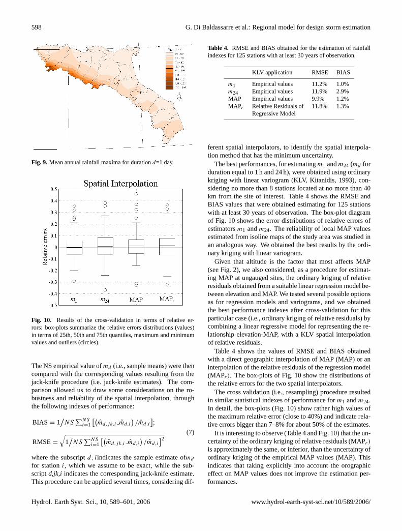
The estimation of the design storm, for durationd, at un-gauged sites requires an estimate of the index storm,md .This is a crucial step. The direct estimation ofmd for an un-gauged site is clearly impossible. Isoline maps ofmd ob-tained with an adequate spatial interpolator, can be used in-stead (see e.g., Brath et al., 2003). Some isoline maps arereported in Figs. 7, 8 and 9. The indirect estimation of MAPis also essential for applying the proposed regional modelto ungauged sites, as it clearly appears from Eq. (6). Alsothe local MAP value can be retrieved at ungauged sites fromisoline maps. Therefore, indications on the uncertainty as-sociated with standard spatial interpolation procedures are

Fig. 7. Mean annual rainfall maxima for durationd=15 min.

Fig. 8. Mean annual rainfall maxima for durationd=1 h.

very important. We report here the results of a series of re-sampling experiments aiming at assessing the reliability ofmd and MAP estimates based upon isoline maps. The re-sampling experiments (jack-knife procedure, see Brath et al.,2003) are structured as follows:

1. we considered the durationd and the numberNS ofavailable raingauges where it was possible to calculatemd from the series of annual maximum depth with du-rationd (sample mean of annual rainfall maxima);

2. one of these raingauges, say station i, and its corre-spondingmd value were removed from the set;

3. we generate a isopluvial map ofmd , interpolating thedata of the remainingNS-1 raingauges sites;

4. a jack-knife estimate ofmd for site i was then retrievedfrom the map identified at step 3;

5. steps 2–4 were repeatedNS-1 times, considering in turnone of the remaining raingauges.



Fig. 9. Mean annual rainfall maxima for durationd=1 day.

Fig. 10. Results of the cross-validation in terms of relative er-rors: box-plots summarize the relative errors distributions (values)in terms of 25th, 50th and 75th quantiles, maximum and minimumvalues and outliers (circles).

The NS empirical value ofmd (i.e., sample means) were thencompared with the corresponding values resulting from thejack-knife procedure (i.e. jack-knife estimates). The com-parison allowed us to draw some considerations on the ro-bustness and reliability of the spatial interpolation, throughthe following indexes of performance:

BIAS = 1/NS

∑NSi=1

[(m̂d,jk,i m̂d,i

)/m̂d,i

];

RMSE=

√1/NS

∑NSi=1

[(m̂d,jk,i m̂d,i

)/m̂d,i

]2(7)

where the subscriptd, iindicates the sample estimate ofmd

for stationi, which we assume to be exact, while the sub-scriptd,jk,i indicates the corresponding jack-knife estimate.This procedure can be applied several times, considering dif-

Table 4. RMSE and BIAS obtained for the estimation of rainfallindexes for 125 stations with at least 30 years of observation.

KLV application RMSE BIAS

m1 Empirical values 11.2% 1.0%m24 Empirical values 11.9% 2.9%MAP Empirical values 9.9% 1.2%MAPr Relative Residuals of 11.8% 1.3%

Regressive Model

ferent spatial interpolators, to identify the spatial interpola-tion method that has the minimum uncertainty.

The best performances, for estimatingm1 andm24 (md forduration equal to 1 h and 24 h), were obtained using ordinarykriging with linear variogram (KLV, Kitanidis, 1993), con-sidering no more than 8 stations located at no more than 40km from the site of interest. Table 4 shows the RMSE andBIAS values that were obtained estimating for 125 stationswith at least 30 years of observation. The box-plot diagramof Fig. 10 shows the error distributions of relative errors ofestimatorsm1 andm24. The reliability of local MAP valuesestimated from isoline maps of the study area was studied inan analogous way. We obtained the best results by the ordi-nary kriging with linear variogram.

Given that altitude is the factor that most affects MAP(see Fig. 2), we also considered, as a procedure for estimat-ing MAP at ungauged sites, the ordinary kriging of relativeresiduals obtained from a suitable linear regression model be-tween elevation and MAP. We tested several possible optionsas for regression models and variograms, and we obtainedthe best performance indexes after cross-validation for thisparticular case (i.e., ordinary kriging of relative residuals) bycombining a linear regressive model for representing the re-lationship elevation-MAP, with a KLV spatial interpolationof relative residuals.

Table 4 shows the values of RMSE and BIAS obtainedwith a direct geographic interpolation of MAP (MAP) or aninterpolation of the relative residuals of the regression model(MAPr). The box-plots of Fig. 10 show the distributions ofthe relative errors for the two spatial interpolators.

The cross validation (i.e., resampling) procedure resultedin similar statistical indexes of performance form1 andm24.In detail, the box-plots (Fig. 10) show rather high values ofthe maximum relative error (close to 40%) and indicate rela-tive errors bigger than 7–8% for about 50% of the estimates.

It is interesting to observe (Table 4 and Fig. 10) that the un-certainty of the ordinary kriging of relative residuals (MAPr)

is approximately the same, or inferior, than the uncertainty ofordinary kriging of the empirical MAP values (MAP). Thisindicates that taking explicitly into account the orographiceffect on MAP values does not improve the estimation per-formances.




The results are obviously connected with the consideredstudy area and raingauge network. Nevertheless, the anal-ysis quantifies effectively (see Table 4 and Fig. 10) the un-certainty ofmd and MAP from isoline maps, showing thatthe reliability level is analogous for all considered rainfallindexes (i.e.,m1, m24 and MAP) and depends on the geosta-tistical spatial interpolator.

5.3 Uncertainty of the regional estimates

We evaluated the performance of the regional model througha comprehensive jack-knife cross-validation (see e.g., Brathet al., 2001). The cross-validation procedure enabled us tocompare the regional and resampled estimates of the designstorm at all considered raingauges for two arbitrarily selectedduration: 1 and 24 h and two reference recurrence intervals:100 and 200 yrs, which are normally adopted in Italy for de-signing flood risk mitigation measures. Through this com-parison we quantified the uncertainty of the design storm es-timates that can be computed by applying the proposed re-gional model to any ungauged site within the study area. Inparticular, we compared the regional estimate of the dimen-sionless growth factor,h′(d,T ), and design storm,h(d,T ),with their resampled counterparts,h′

jk(d,T ) and hjk(d,T ),respectively. We computedh′

jk(d, T ) andhjk(d,T ) as fol-lows:

1. one of the NS raingauges, say stationi, and its corre-sponding data were removed from the set;

2. parametersa, b andc of model (6) were estimated onthe basis of the pluviometric information collected atthe remaining NS-1 raingauges;


3. jack-knifed regional L-moments, L-CvRjk and L-CsRjk,were calculated for sitei by using the recalibratedmodel (7) identified at step 2) and the jack-knifedMAP value (MAPjk) retrieved for sitei from isolineMAP generated through ordinary kriging as describedin Sect. 5.2;

4. the jack-knifed parameters of the regional GEV distri-bution were estimated for sitei through the method ofL-moments on the basis of the L-CvRjk and L-CsRjk val-ues estimated at step 3);

5. h′

jk(d,T ) was computed for site i as theT -year quantilefrom the GEV distribution estimated at step 4);

6. hjk(d,T ) was then computed as the product ofh′

jk(d,T)and the jack-knife estimate ofmd , which was calculatedas described in Sect. 5.2;

7. steps 1–6 were repeated NS-1 times, considering in turnone of the remaining raingauges.

The box-plot diagram of Fig. 11 shows the distributionsof relative errors for the estimation of the growth factorh′(1 h,100 yrs) andh′(24 h,100 yrs) and the design stormh(1 h,100 yrs) andh(24 h,100 yrs). Figure 12 shows the dis-tributions of relative errors for the estimation of the growthfactor h′(1 h,200 yrs) andh′(24 h,200 yrs) and the designstormh(1 h,200 yrs) andh(24 h,200 yrs). The figures showthat the application of the proposed regional model to un-gauged sites provides unbiased estimates ofh′(d,T ), for d=1,24 h and T=100, 200 yrs. Also, Figs. 11 and 12 illustrate that



the absolute value of relative errors of the dimensionless re-gional growth factors is generally small and always lowerthan 10%.

It is important to notice that if the local value of MAPis known (e.g., from observed daily rainfall data), then therelative errors ofh′(d,T ) estimates, resulting from the uncer-tainties in the parameters of model (6), become practicallynegligible (<1%).

Concerning the estimation ofh(d,T ) the performance ofthe model is definitely lower than 30%. A comparison be-tween the relative errors of Figs. 11 and 12 points out ratherclearly that the largest uncertainty in the application of theregional model to an ungauged site is associated with theindex-storm estimates (see Sect. 5.2).

The presence of cross correlation between stations doesnot introduce a bias effect, but could increase the uncertaintyof the estimates (see Hosking and Wallis, 1988). These ef-fects are not quantified at this stage, but we are planning toinvestigate this matter in the future.

6 Conclusions

The paper presents a regional frequency analysis of annualmaximum rainfall depths for storm duration ranging from15 min to 1 day, observed for a dense network of raingaugesplaced in northern central Italy.

The study investigates the statistical properties of rainfallextremes using an approach based on L-moments, and de-tects important relations between these statistics and meanannual precipitation (MAP). Previous studies (Schaefer,1990; Alila, 1999) showed that the statistics of rainfall ex-tremes vary systematically with location and these studiesalso identified statistically significant relationships betweenthese statistics and MAP, which was used as a surrogate ofgeographical location. For instance, Schaefer (1990) showedthat the coefficients of variation and skewness of rainfall ex-tremes tend to decrease as the local value of MAP increases.Our study confirmed in part these findings on a different ge-ographic area.

We developed an empirical regional model that enablesone to estimate the design storm in any location of the studyarea. We assessed the model applicability through MonteCarlo experiments and quantified the uncertainty of the es-timates for ungauged sites using an extensive jack-knife re-sampling procedure.

The jack-knife procedure pointed out that the estimates ofthe design storm are basically unbiased and that the appli-cability of the regional model to ungauged sites is rather re-liable. We obtained for the study area resampled estimatesof the design storm characterised by relative errors generallylower that 10% and never higher than 40%. Also, the resam-pling procedure highlighted that the highest uncertainty isassociated with the estimation of the index storm (i.e., meanannual maximum rainfall depth for a given duration).

It is important to underline that the proposed regionalmodel was developed through statistical optimisation. There-fore, that the model itself can be applied to storm durationfrom 15 min to 1 day and sites located within the study area.A careful application of the regional model should also con-sider that the model itself was developed for raingauges lo-cated below 1500 m a.s.l., while the altitude in the study areacan locally exceed 2000 m a.s.l. Finally, the spatial interpola-tion of rainfall extremes or MAP adopted in our study is un-able to reproduce micro-climatic effects such as rain shadoweffects, and can only provide an overly simplified represen-tation of differences existing between leeward and windwardsides of the same mountain depending of the particular spa-tial interpolator adopted in the study.

Appendix A

Homogeneity test

The Hosking and Wallis test assesses the homogeneity of agroup of basins at three different levels by focusing on threemeasures of dispersion for different orders of the sample L-moment ratios (see Hosking (1990) for an explanation of L-moments):

A measure of dispersion for the L-Cv:

V1 =

R∑i=1

ni

(t2(i) − t̄2

)2

/R∑

i=1

ni (A1)

A measure of dispersion for both the L-Cv and the L-Csco-efficients in the L-Cv-L-Csspace:

V2 =

R∑i=1

ni

[(t2(i) − t̄2

)2+

(t3(i) − t̄3

)2]1/2

/R∑

i=1

ni (A2)

A measure of dispersion for both the L-Csand the L-Ck co-efficients in the L-Cs-L-Ck space:

V3 =

R∑i=1

ni

[(t3(i) − t̄3

)2+

(t4(i) − t̄4

)2]1/2

/R∑

i=1

ni (A3)

wheret̄2, t̄3, and t̄4 are the group mean of L-Cv, L-Cs, andL-Ck respectively;t2(i), t3(i), t4(i), andni are the values ofL-Cv, L-Cs, L-Ck and the sample size for sitei; andR is thenumber of sites in the pooling group.

The underlying concept of the test is to measure the sam-ple variability of the L-moment ratios and compare it to thevariation that would be expected in a homogeneous group.The expected mean value and standard deviation of thesedispersion measures for a homogeneous group,µVk

andσVk

respectively, are assessed through repeated simulations,by generating homogeneous groups of basins having thesame record lengths as those of the observed data followingthe methodology proposed by Hosking and Wallis (1993).



The heterogeneity measures are then evaluated using the fol-lowing expression:

H(k) =Vk − µVk

σVk

; for k = 1, 2, 3 (A4)

Hosking and Wallis (1993) suggested that the region or groupof sites should be considered as acceptably homogeneous ifH<1; possibly heterogeneous if 1≤H<2, and definitely het-erogeneous if H≥2.

Acknowledgements.The study presented here has been carriedout in the framework of the activity of the Working Group onthe Characterisation of Ungauged Basins by Integrated uSe ofhydrological Techniques (CUBIST). The work has been partiallysupported by the Italian Ministry of University and Research inScience and Technology (MURST). We would like to thank theAssociate Editor, P. Molnar, and the Reviewers, P. Bernardara andY. Alila, for providing very useful comments, which helped us inimproving the presentation of our work.

Edited by: P. Molnar

References

Alila, Y.: A hierarchical approach for the regionalization of precipi-tation annual maxima in Canada, J. Geophys. Res., 104, 31 645–31 655, 1999.

Brath, A. and Franchini, M.: La valutazione delle Pioggie intensesu base regionale (in Italian), in: L’ingegneria naturalistica nellasistemazione dei corsi d’acqua, edited by: Maione, U. and Brath,A., BIOS (Cosenza), 65–91, 1999.

Brath, A. and Franchini, M.: la valutazione delle pioggie intense subase regionale (in Italian),Proceedings of the scientific seminarL’ingegneria naturalistica nella sistemazione dei corsi d’acqua,edited by: Maione, U. and Brath, A., BIOS (Cosenza), 65–91,1999.

Brath, A. and Castellarin, A.: Tecniche di affinamento delle previ-sioni regionali del rischio pluviometrico (in Italian), Proceedingsof the scientific seminar La progettazione della difesa idraulica –Interventi di laminazione controllata delle piene fluviali, editedby: Maione, U., Brath, A., and Mignosa, P., BIOS (Cosenza),93–121, 2001.

Brath, A., Castellarin, A., and Montanari, A.: Assessing the reli-ability of regional depth-duration-frequency equations for gagedand ungaged sites, Water Resour. Res., 39(12), 1367–1379, 2003.

Burlando, P. and Rosso, R.: Scaling and multiscaling Depth-Duration-Frequency curves of storm precipitation, J. Hydrol.,187, 45–64, 1996.

Burn, D. H.: Evaluation of regional flood frequency analysis with aregion of influence approach, Water Resour. Res., 26(10), 2257–2265, 1990.

Castellarin, A., Burn, D. H., and Brath, A.: Assessing the effec-tiveness of hydrological similarity measures for flood frequencyanalysis, J. Hydrol., 241(3–4), 270–285, 2001.

Castellarin, A. and Brath, A.: Tecniche di perfezionamento dellestime regionali del rischio pluviometrico (in Italian), Proceedingsof the XXVIII Italian Conference on Hydraulics and HydraulicWorks, Potenza 16–19 settembre 2002, 1, 225–236, Ed. BIOS,Cosenza, 2002.

Castellarin, A. and Brath, A.: Descriptive capability of seasonalityindicators for regional frequency analyses of flood and rainfall,Proceedings of the International Conference on Flood Estima-tion, CHR Rep. II-17, 429–440, Lelystad, Netherlands, 2002.

Dalrymple, T.: Flood frequency analysis, U.S. Geol. Surv. WaterSupply Pap., 1543-A, 11–51, 1960.

Faulkner, D.: Rainfall frequency estimation, Flood estimationHandbook, 2, Wallingford, 1999.

Franchini, M. and Galeati, G.: La regionalizzazione delle pioggieintense mediante il modello TCEV. Una applicazione alla regioneRomagna-Marche (in Italian), Idrotecnica, 5, 1994.

Gabriele, S. and Arnell, N.: A hierarchical approach to regionalflood frequency analysis, Water Resour. Res., 27(6), 1281–1289,1991.

Horton, R. E.: Analysis of runoff-plat experiments with varying in-filtration capacity. Transactions, Am. Geophys. Union, 20, 693–711, 1939.

Hosking, J. R. M.: L-moments: analysis and estimation of distribu-tions using linear combination of order statistics, J. Royal Statis-tical Soc., Series B., 52(1), 105–124, 1990.

Hosking, J. R. M. and Wallis, J. R.: The Effect of Inter-Site De-pendence on Regional Flood Frequency Analysis, Water Resour.Res., 24, 588–600, 1988.

Hosking, J. R. M. and Wallis, J. R.: Some statistics useful in re-gional frequency analysis, Water Resour. Res., 29(2), 271–281,1993.

Hosking, J. R. M. and Wallis, J. R.: Regional frequency Analysis,Cambridge University Press, New York, 1997.

Jenkinson, A. F.: The frequency distribution of the annual maxi-mum (or minimum) of meteorological elements, Q. J. Royal Me-teorol. Soc., 81, 1955.

Kitanidis, P. K.: Geostatistics, Handbook of Hydrology, edited by:Maidment, D. R., McGraw-Hill, New York, 20.1–20.39, 1993.

Klemes V.: Tall tales about tails of hydrological distributions: I andII, J. Hydrol. Eng., American Society of Civil Engineers 5(3),227–239, 2000.

Marani, M.: On the correlation structure of continuous anddiscrete point rainfall, Water Resour. Res., 39(5), 1128,doi:10.1029/2002WR001456, 2003.

Olsson, J. and Burlando, P.: Reproduction of temporal scaling bya rectangular pulses rainfall model, Hydrol. Processes, 16, 611–630, 2002.

Schaefer, M. G.: Regional analyses of precipitation annual maximain Washington State, Water Resour. Res., 26(1), 119–131, 1990.

Schaefer, M. G.: Regional analyses of precipitation annual maximain Washington State, Water Resour. Res., 26(1), 119–131, 1990.


relationships between statistics of rainfall extremes and mean

Documents