reduction of combustion noise and instabilities a...
TRANSCRIPT

REDUCTION OF COMBUSTION NOISE AND INSTABILITIES
USING POROUS INERT MATERIAL WITH
A SWIRL-STABILIZED BURNER
by
DANIEL SEQUERA
A DISSERTATION
Submitted in partial fulfillment of the requirements for the degree of Doctor of Philosophy
in the Department of Mechanical Engineering in the Graduate School of
The University of Alabama
TUSCALOOSA, ALABAMA
2011

Copyright Daniel Sequera 2011 ALL RIGHTS RESERVED

ii
ABSTRACT
Combustion instabilities represent a major problem during operation of power generation
systems that can lead to costly shutdown. Combustion instabilities are self excited large
amplitude pressure oscillations caused by the coupling of unsteady heat release and acoustic
modes of the combustor. These oscillations cause fluctuating mechanical loads and fluctuating
heat transfer that can result in catastrophic premature failure of components. Combustion noise, a
significant source of noise in gas turbines, can lead to combustion instabilities. Combustion noise
and instabilities are different phenomena; however, they both occur due to unsteady heat release
of turbulent flames that excites acoustic modes of the combustor. The instabilities self excite
when flame adds energy to the acoustic field at a faster rate than it can dissipate it. Swirl-
stabilized combustion and porous inert medium (PIM) combustion are two methods that have
extensively been used, although independently, for flame stabilization. In this study, the two
concepts are combined so that PIM serves as a passive device to mitigate combustion noise and
instabilities. A PIM insert is placed within the lean premixed, swirl-stabilized combustor to
affect the turbulent flow field reducing combustion noise. This study is the first step for eventual
implementation in liquid fuel systems. After presenting the concept, a numerical investigation of
the changes in the mean flow field caused by the PIM is presented. Changes in the flow field can
be beneficial for noise reduction by optimizing the geometric parameters of the PIM. Next,
atmospheric pressure experiments were conducted at low reactant inlet velocity (<10 m/s) and
low reactant inlet temperature (<120 °C) to investigate effect of PIM parameters on sound

iii
pressure level (SPL), and CO and NOx emissions. Surface and interior combustion modes were
identified and PIM geometric parameters were optimized. Next, a laboratory facility to conduct
experiments at high reactant inlet velocity, high inlet air temperature, and high pressure was
designed and developed. Results show that the porous insert substantially reduces combustion
noise for a range of operating conditions. Moreover, experiments show that the porous insert can
mitigate combustion instabilities without adversely affecting CO and NOx emissions.

iv
DEDICATION
This dissertation is dedicated to all my family, particularly to my parents, Yelitza and
Edgar, and my brothers, Axzel and Reinaldo.

v
LIST OF ABREVIATIONS AND SYMBOLS
A Model constant
AA Atomizing air
B Bias uncertainty �̃ Mean reaction progress variable
CD Turbulent length scale constant
C0 Model constant
C1 Model constant
CO Carbon monoxide
FFT Fast Fourier transform
FPGA Field-programmable gate array
HfC Hafnium Carbide
ID Inside diameter
k Turbulent kinetic energy
keff Effective thermal conductivity
Li ith acoustic energy loss process
LFE Laminar flow element
LPM Lean premixed
lpm Liters per minute

vi
lnpm Normal liters per minute
l t Turbulent length scale
n Number of products
NOx Nitrogen oxides
NG Natural gas
OD Outside diameter
PIM Porous inert medium
P Random uncertainty
Prms Root mean square of pressure
Pchamber Pressure inside enclosure
Pinlet Pressure at inlet
Pref Reference pressure
ppm Parts per million
p’ Combustor pressure oscillations
Q Combustion air flow rate
Qc Cooling air flow rate
q’ Heat addition oscillations
Re Reynolds number
RNG Renormalization group
RT Real time
Sc Mean reaction rate
Sct Turbulent Schmidt number
Si Momentum sink term
vii
SiC Silicon Carbide
slpm Standard liters per minute
SPL Sound pressure level
T Period of oscillations
Ti Inlet temperature
U Velocity
u’ RMS velocity
Ui Overall uncertainty
Ul Laminar flame speed
Ut Turbulent flame speed
V Combustor volume �� Velocity vector
Yi Mass fraction of product species i
Yi, eq Equilibrium mass fraction of product species i � Thermal diffusivity of unburnt mixture � Turbulence dissipation rate
Ф Equivalence ratio
µt Turbulent viscosity
µeff Effective viscosity � Density
ρu Density of unburnt mixture

viii
ACKNOWLEDGMENTS
I would like to take this opportunity to show my appreciation to everyone that directly and
indirectly had a contribution to make this dissertation possible.
First and foremost, I want to express my most sincere appreciation to my academic
advisor and friend, Dr. Ajay K. Agrawal, whose guidance throughout my studies made my
experience in Tuscaloosa one that I will always cherish. His technical knowledge and managerial
skills, patience and professional attitude towards any situation, even the most difficult ones,
taught me invaluable lessons and greatly influenced my professional growth. Moreover, his
ability to be demanding yet appreciative, his opportunistic advice, inside and outside the
academic environment, made my graduate studies absolutely enjoyable.
I want to gratefully thank all members of my committee, Dr. Baker, Dr. Olcmen, Dr.
Taylor and Dr. Wiest, excellent engineers I am privileged to have had as professors.
Next, I want to express my special gratitude to fellow graduate students I had the fortune
to go to class and share with. Heena, Pankaj, Ben, Troy, Tanisha, Justin, Lulin, Cristina, Cosmin,
and Vijay were always helpful, supportive and fun to enjoy conversation with over a cup of
coffee. I also want to express particular gratitude to Zach, whom I had the chance to work with in
the final stages of my studies. Completion of this investigation was only possible with his
unconditional and assertive support. I also want to express my gratitude to all staff members in
the Mechanical Engineering Department, whose dedication and professionalism make possible

ix
for students to successfully complete academic careers at UA. Lynn, Pamelia, Betsy, Lisa, Barry,
Ken, Jim, Sam, James, thank you all very much.
I also want to thank my good friends Paulo, Amanda, Jose, Troy, my cousin Miguel and
my brothers Axzel and Reinaldo for making my stay in Tuscaloosa unforgettable, for always
being supportive, encouraging, and fun to be around. Needless to say, I will be forever grateful to
my parents for all the support, guidance, help and unconditional love during my time in UA.

x
CONTENTS
ABSTRACT ...................................................................................................................... ii
DEDICATION ................................................................................................................. iv
LIST OF ABREVIATIONS AND SYMBOLS .................................................................. v
ACKNOWLEDGMENTS .............................................................................................. viii
LIST OF TABLES ......................................................................................................... xiv
LIST OF FIGURES ........................................................................................................ xvi
1. INTRODUCTION ....................................................................................................... 1
1.1 Background ............................................................................................................ 1
1.2 Overview ................................................................................................................ 4
2. NUMERICAL SIMULATIONS OF SWIRL STABILIZED COMBUSTION COUPLED WITH POROUS INERT MEDIUM .......................................................... 9
2.1 Background ............................................................................................................ 9
2.2 Physical Model ..................................................................................................... 11
2.2.1 Governing Equations ................................................................................... 11
2.2.2 Combustion Model ....................................................................................... 12
2.2.3 Boundary Conditions ................................................................................... 14
2.2.4 Model Validation ......................................................................................... 15
2.3 Results and Discussion ........................................................................................ 16
2.3.1 Non-Reacting Flow ...................................................................................... 16
xi
2.3.2 Reacting Flow ............................................................................................. 17
2.4 Conclusions .......................................................................................................... 19
3. NOISE REDUCTION IN SWIRL-STABILIZED COMBUSTOR COUPLED WITH PIM ..................................................................... 38
3.1 Background ......................................................................................................... 38
3.2 Experimental Setup .............................................................................................. 40
3.3 Results and Discussion ........................................................................................ 42
3.3.1 Effect of PIM Pore Density .......................................................................... 44
3.3.2 Effect of PIM Geometry ............................................................................... 46
3.3.3 Effect of Reactant Flow Rate ........................................................................ 47
3.3.4 CO and NOx Emissions ................................................................................ 49
3.3.5 Long Duration Experiments ......................................................................... 50
3.4 Conclusions .......................................................................................................... 51
4. DEVELOPMENT OF A FACILITY FOR HIGH FLOW RATE, HIGH INLET TEMPERATURE, AND HIGH PRESSURE COMBUSTION EXPERIMENTS ........ 78
4.1 Background ......................................................................................................... 78
4.2 Reactant Supply Systems ..................................................................................... 80
4.2.1 Air Lines ...................................................................................................... 80
4.2.2 Electric Heater ............................................................................................ 82
4.2.3 Fuel Line ..................................................................................................... 82
4.2.4 Product Exhaust Line .................................................................................. 83
4.3 Instruments and Data Acquisition System ............................................................ 84
4.4 Combustion Experimental Apparatus ................................................................... 87

xii
5. REDUCTION OF COMBUSTION NOISE AND INSTABILITIES WITH THE USE OF POROUS INERT MATERIAL .............................................. 120
5.1 Background ....................................................................................................... 120
5.2 Experimental Setup ............................................................................................ 122
5.3 Results and Discussion ...................................................................................... 126
5.3.1 Open Top Experiments ............................................................................... 130
a. Effect of Pore Density ......................................................................... 130
b. Effect of Flow Rate ............................................................................... 134
5.3.2 Restricted Top Experiments........................................................................ 137
a. Effect of PIM on Noise at P = 1 atm .................................................... 137
b. Effect of PIM on Noise at P = 2 atm ..................................................... 143
5.4 Conclusions ........................................................................................................ 145
6. CONCLUSIONS AND RECOMMENDATIONS .................................................... 220
6.1 Conclusions ....................................................................................................... 220
6.2 Recommendations .............................................................................................. 222
REFERENCES .............................................................................................................. 224
APPENDIX A COMBUSTION PERFORMANCE OF LIQUID BIO-FUELS IN A SWIRL STABILIZED BURNER ...................................... 229
APPENDIX B CALCULATION OF SWIRL NUMBER ............................................... 258
APPENDIX C CALCULATION OF AIR FLOW RATE IN LFE .................................. 260
APPENDIX D SAMPLE CALCULATIONS OF O2 AND CO2 CONCENTRATIONS .............................................................................. 263
APPENDIX E FLOW VELOCITY AND REYNOLDS NUMBER CALCULATIONS........................................................................................ 266

xiii
APPENDIX F SOUND PRESSURE LEVEL CALCULATION SCRIPT ............................................................................................. 268
UNCERTAINTY ANALYSIS ....................................................................................... 274
xiv
LIST OF TABLES
3.1 Summary of results, effect of pore density, Q = 300 slpm ..................................... 45
3.2 Summary of results, effect of geometry, Q = 300 slpm ........................................ 48
3.3 Summary of results, effect of flow rate ................................................................. 49
3.4 Summary of SPL for long-duration experiment .................................................... 51
4.1 Air supply line parts ............................................................................................. 81
4.2 Fuel supply line parts............................................................................................ 84
4.3 List of instruments for flow measurement ............................................................. 85
5.1 Effect of microphone location on SPL for open top experiments, Q = 1020 slpm, Ф = 0.7, Tinlet = 20 °C ................................................................ 128
5.2 Effect of microphone location on SPL for restricted top experiments, Q = 1020 slpm, Ф = 0.7, Tinlet = 20 °C, Qc = 990 slpm ........................................ 129
5.3 Summary of sound pressure levels for Q = 1020 slpm ........................................ 133
5.4 Summary of pressure measurements for Q = 1020 slpm...................................... 134
5.5 Summary of sound pressure levels for Q = 1400 slpm ........................................ 136
5.6 Summary of pressure measurements for Q = 1400 slpm...................................... 137
5.7 Summary of jet noise total SPL, Q = 1020 slpm, P = 1 atm ................................. 141
5.8 Summary of combustion noise total SPL, Q = 1020 slpm, P = 1 atm................... 142
5.9 Summary of pressure measurements for restricted top experiments, Q = 1020 slpm, P = 1 atm ........................................................ 143

xv
5.10 Summary of Combustion Noise total SPL, Q = 2040 slpm, P = 2 atm ................. 144
5.11 Summary of pressure measurements for restricted top experiments, Q = 2040 slpm, P = 2 atm ........................................................ 145
A.1 NREL biooil characteristics ................................................................................ 233
A.2 Experimental fuel blends (Vol%) ........................................................................ 233
A.3 Water contents in the fuel blend.......................................................................... 234
C.1 Calibration coefficients for air flow rate calculation............................................ 261
D.1 Summary of O2 and CO2 calculated and experimental results ............................. 265
E.1 Summary of flow velocity and Reynolds number calculations ............................ 267
G.1 Readings for air and fuel random uncertainty calculation, low pressure facility ........................................................................................... 277
G.2 Readings for air and fuel random uncertainty calculation, high pressure facility .......................................................................................... 278
G.3 Readings for pressure random uncertainty calculation, high pressure facility .......................................................................................... 279
xvi
LIST OF FIGURES
1.1 Schematic diagram of swirl stabilization mechanism ............................................. 7
1.2 Proposed concepts .................................................................................................. 8
2.1 Schematic diagram of swirl stabilization mechanism ........................................... 21
2.2 Schematic of combustor with the swirler .............................................................. 22
2.3 Computational domain ......................................................................................... 23
2.4 Axial velocity profile at z = 20 mm, methane flame, Φ = 0.58 .............................. 23
2.5 Velocity vectors for non-reacting flow. (a) Experimental results (Wicksall, 2005), (b) Computed results................................................................. 24
2.6 Velocity vectors for reacting flow. (a) Experimental results (Wicksall, 2005), (b) Computed results................................................................. 25
2.7 Velocity vectors for non-reacting flow. (a) without PIM, (b) with PIM ................. 26
2.8 Axial velocity profiles at different axial locations for non-reacting flow: (a) z =10 mm, (b) 20 = mm, (c) 30 = mm ........................... 27
2.9 Swirl velocity profiles at different axial locations for non-reacting flow: (a) z =10 mm, (b) 20 = mm, (c) 30 = mm ........................... 28
2.10 Radial velocity profiles at different axial locations for non-reacting flow: (a) z =10 mm, (b) 20 = mm, (c) 30 = mm ........................... 29
2.11 Velocity vectors for reacting flow Ф = 0.58. (a) without PIM, (b) with PIM ......... 30
2.12 Axial velocity profiles at different axial locations for Ф = 0.58: (a) z =10 mm, (b) 20 = mm, (c) 30 = mm ........................................ 31
2.13 Swirl velocity profiles at different axial locations for Ф = 0.58: (a) z =10 mm, (b) 20 = mm, (c) 30 = mm ........................................ 32
xvii
2.14 Radial velocity profiles at different axial locations for Ф = 0.58: (a) z =10 mm, (b) 20 = mm, (c) 30 = mm ........................................ 33
2.15 Velocity vectors for reacting flow Ф = 0.85. (a) without PIM, (b) with PIM ......... 34
2.16 Axial velocity profiles at different axial locations for Ф = 0.85: (a) z =10 mm, (b) 20 = mm, (c) 30 = mm ........................................ 35
2.17 Swirl velocity profiles at different axial locations for Ф = 0.85: (a) z =10 mm, (b) 20 = mm, (c) 30 = mm ........................................ 36
2.18 Radial velocity profiles at different axial locations for Ф = 0.85: (a) z =10 mm, (b) 20 = mm, (c) 30 = mm ........................................ 37
3.1 Schematic diagram of experimental setup ............................................................. 52
3.2 Photos of PIM inserts (a) PIM insert (b) combustor without PIM (c) combustor with two PIM pieces ...................................................................... 53
3.3 Description and schematic diagram of PIM configurations used in this study........ 54
3.4 Flame images, (a) without PIM (b) with PIM interior combustion (c) with PIM surface combustion .......................................................................... 55
3.5 Schematic diagram illustrating the PIM stabilization mechanism .......................... 56
3.6 One third octave band SPL for repeatability test ................................................... 57
3.7 Flame images for Q = 300 slpm, Ф = 0.7 (a) Configuration A (b) Configuration B (c) Configuration C (d) Configuration D (e) Configuration E (f) Configuration F (g) Configuration G (h) Configuration h (i) Configuration I ................................................................. 58
3.8 Flame images for Q = 300 slpm, Ф = 0.8 (a) Configuration A (b) Configuration B (c) Configuration C (d) Configuration D (e) Configuration E (f) Configuration F (g) Configuration G (h) Configuration h (i) Configuration I ................................................................. 59
3.9 Power spectra for Q = 300 slpm, Ф = 0.7 (a) Configuration A (b) Configuration B (c) Configuration C (d) Configuration D (e) Configuration E (f) Configuration F (g) Configuration G (h) Configuration h (i) Configuration I ................................................................. 60
xviii
3.10 Power spectra for Q = 300 slpm, Ф = 0.8 (a) Configuration A (b) Configuration B (c) Configuration C (d) Configuration D (e) Configuration E (f) Configuration F (g) Configuration G (h) Configuration h (i) Configuration I ................................................................. 61
3.11 One third octave band SPL, effect of pore density, Q = 300 slpm (a) Ф = 0.7 (b) Ф = 0.8 ......................................................................................... 62
3.12 One third octave band SPL, effect of geometry, Q = 300 slpm (a) Ф = 0.7 (b) Ф = 0.8 ......................................................................................... 63
3.13 Flame images for Q = 300 slpm, Ф = 0.7 (a) Configuration A (b) Configuration D (c) Configuration G (d) Configuration I ................................ 64
3.14 Flame images for Q = 300 slpm, Ф = 0.8 (a) Configuration A (b) Configuration D (c) Configuration G (d) Configuration I ................................ 65
3.15 Flame images for Q = 600 slpm, Ф = 0.7 (a) Configuration A (b) Configuration D (c) Configuration G (d) Configuration I ................................ 66
3.16 Flame images for Q = 600 slpm, Ф = 0.8 (a) Configuration A (b) Configuration D (c) Configuration G (d) Configuration I ................................ 67
3.17 Power spectra for Q = 600 slpm, Ф = 0.7 (a) Configuration A (no PIM) (b) Configuration D (divergent) (c) Configuration G (constant) (d) Configuration I (convergent) ........................... 68
3.18 Power spectra for Q = 600 slpm, Ф = 0.8 (a) Configuration A (no PIM) (b) Configuration D (divergent) (c) Configuration G (constant) (d) Configuration I (convergent) ........................... 69
3.19 One third octave band SPL, effect of reactants flow rate, Q = 300 slpm (a) Ф = 0.7 (b) Ф = 0.8 ................................................................... 70
3.20 One third octave band SPL, effect of reactants flow rate, Q = 600 slpm (a) Ф = 0.7 (b) Ф = 0.8 ................................................................... 71
3.21 CO and NOx emissions for Q = 300 slpm, Ф = 0.7, Ti = 100 °C (a) CO (b) NOx ................................................................................. 72
3.22 CO and NOx emissions for Q = 300 slpm, Ф = 0.8, Ti = 100 °C (a) CO (b) NOx ................................................................................. 73
3.23 CO and NOx emissions for Q = 600 slpm, Ф = 0.7, Ti = 100 °C (a) CO (b) NOx ................................................................................. 74

xix
3.24 CO and NOx emissions for Q = 600 slpm, Ф = 0.8, Ti = 100 °C (a) CO (b) NOx ................................................................................. 75
3.25 One third octave band SPL, long duration test ...................................................... 76
3.26 CO and NOx emissions for Q = 600 slpm, Ф = 0.7, long duration test (a) CO (b) NOx ........................................................................ 77
4.1 General schematic of high pressure combustion laboratory ................................... 91
4.2 Layout of air flow control system ......................................................................... 92
4.3 Layout of high pressure combustion laboratory .................................................... 93
4.4 Layout of high pressure combustion laboratory .................................................... 94
4.5 (a) Photographic image of combustion air pre-heater (b) Schematic diagram of combustion air pre-heater ............................................. 95
4.6 Heater stand ......................................................................................................... 96
4.7 Fuel station ........................................................................................................... 97
4.8 Layout of fuel flow control system ....................................................................... 98
4.9 Exhaust side view ................................................................................................. 99
4.10 Exhaust overhead view ....................................................................................... 100
4.11 Exhaust front view.............................................................................................. 101
4.12 CompactRIO system ........................................................................................... 102
4.13 Sensor/controller and CompactRIO layout .......................................................... 103
4.14 Schematic of assembled experimental apparatus ................................................. 104
4.15 Exploded view of experimental apparatus ........................................................... 105
4.16 Photographic image of experimental apparatus ................................................... 106
4.17 Photographic image of experimental apparatus ................................................... 107
4.18 Photographic image of experimental apparatus ................................................... 108
4.19 Details of assembled plenum base ...................................................................... 109

xx
4.20 Details of support pipe/flange ............................................................................. 110
4.21 Details of plenum base ....................................................................................... 111
4.22 Details of enclosure ............................................................................................ 112
4.23 Details of faces of enclosure ............................................................................... 113
4.24 Details of cross section of enclosure ................................................................... 114
4.25 Details of windows on enclosure ........................................................................ 115
4.26 Details of ports on enclosure............................................................................... 116
4.27 Details of window covers ................................................................................... 117
4.28 Details of windows ............................................................................................. 118
4.29 Schematic diagram and photograph of sampling probe ....................................... 119
5.1 Schematic of experimental setup ........................................................................ 147
5.2 Photograph of fuel station ................................................................................... 148
5.3 Schematic of combustion chamber ..................................................................... 149
5.4 Swirler ............................................................................................................... 150
5.5 Schematic of experimental setup ........................................................................ 151
5.6 Schematic diagram of PIM ................................................................................. 152
5.7 Schematic diagram and photograph of sampling probe ....................................... 153
5.8 Schematic of PIM stabilization mechanism......................................................... 154
5.9 Microphone locations for open top experiments .................................................. 155
5.10 One third octave band SPL for repeatability test ................................................ 156
5.11 Effect of probe position on SPL for open top experiments, Q = 1020 slpm, Ф = 0.7, Tinlet = 20 °C ................................................................ 157
5.12 Microphone locations for restricted top experiments ........................................... 158
xxi
5.13 Effect of microphone location on SPL for restricted top experiments, Q = 1020 slpm, Ф = 0.7, Tinlet = 20 °C, Qc = 990 slpm ........................................ 159
5.14 Power spectra for Q = 1020 slpm, Ф = 0.65, no PIM (a) Tinlet = 20 °C, (b) Tinlet = 130 °C, (c) Tinlet = 260 °C................................................................... 160
5.15 Power spectra for Q = 1020 slpm, Ф = 0.70, no PIM (a) Tinlet = 20 °C, (b) Tinlet = 130 °C, (c) Tinlet = 260 °C................................................................... 161
5.16 Power spectra for Q = 1020 slpm, Ф = 0.75, no PIM (a) Tinlet = 20 °C, (b) Tinlet = 130 °C, (c) Tinlet = 260 °C................................................................... 162
5.17 Power spectra for Q = 1020 slpm, Ф = 0.65, 18 ppcm PIM (a) Tinlet = 20 °C, (b) Tinlet = 130 °C, (c) Tinlet = 260 °C................................................................... 163
5.18 Power spectra for Q = 1020 slpm, Ф = 0.70, 18 ppcm PIM (a) Tinlet = 20 °C, (b) Tinlet = 130 °C, (c) Tinlet = 260 °C................................................................... 164
5.19 Power spectra for Q = 1020 slpm, Ф = 0.75, 18 ppcm PIM (a) Tinlet = 20 °C, (b) Tinlet = 130 °C, (c) Tinlet = 260 °C................................................................... 165
5.20 Power spectra for Q = 1020 slpm, Ф = 0.65, 32 ppcm PIM (a) Tinlet = 20 °C, (b) Tinlet = 130 °C, (c) Tinlet = 260 °C................................................................... 166
5.21 Power spectra for Q = 1020 slpm, Ф = 0.70, 32 ppcm PIM (a) Tinlet = 20 °C, (b) Tinlet = 130 °C, (c) Tinlet = 260 °C................................................................... 167
5.22 Power spectra for Q = 1020 slpm, Ф = 0.75, 32 ppcm PIM (a) Tinlet = 20 °C, (b) Tinlet = 130 °C, (c) Tinlet = 260 °C................................................................... 168
5.23 SPL in one third octave for Q = 1020 slpm, Ф = 0.65, (a) Tinlet = 20 °C, (b) Tinlet = 130 °C, (c) Tinlet = 260 °C................................................................... 169
5.24 SPL in one third octave for Q = 1020 slpm, Ф = 0.70, (a) Tinlet = 20 °C, (b) Tinlet = 130 °C, (c) Tinlet = 260 °C................................................................... 170
5.25 SPL in one third octave for Q = 1020 slpm, Ф = 0.75, (a) Tinlet = 20 °C, (b) Tinlet = 130 °C, (c) Tinlet = 260 °C................................................................... 171
5.26 CO emissions for Q = 1020 slpm, Ф = 0.65, (a) Tinlet = 20 °C, (b) Tinlet = 130 °C, (c) Tinlet = 260 °C................................................................... 172
5.27 CO emissions for Q = 1020 slpm, Ф = 0.75, (a) Tinlet = 20 °C, (b) Tinlet = 130 °C, (c) Tinlet = 260 °C................................................................... 173

xxii
5.28 NOx emissions for Q = 1020 slpm, Ф = 0.65, (a) Tinlet = 20 °C, (b) Tinlet = 130 °C, (c) Tinlet = 260 °C................................................................... 174
5.29 NOx emissions for Q = 1020 slpm, Ф = 0.75, (a) Tinlet = 20 °C, (b) Tinlet = 130 °C, (c) Tinlet = 260 °C................................................................... 175
5.30 Pressure drop measurements for open top experiments Q = 1020 slpm (a) no PIM (b) 18 ppcm PIM (c) 32 ppcm PIM .................................................. 176
5.31 Power spectra for Q = 1400 slpm, Ф = 0.65, no PIM (a) Tinlet = 20 °C, (b) Tinlet = 130 °C, (c) Tinlet = 260 °C................................................................... 177
5.32 Power spectra for Q = 1400 slpm, Ф = 0.70, no PIM (a) Tinlet = 20 °C, (b) Tinlet = 130 °C, (c) Tinlet = 260 °C................................................................... 178
5.33 Power spectra for Q = 1400 slpm, Ф = 0.75, no PIM (a) Tinlet = 20 °C, (b) Tinlet = 130 °C, (c) Tinlet = 260 °C................................................................... 179
5.34 Power spectra for Q = 1400 slpm, Ф = 0.65, 18 ppcm PIM (a) Tinlet = 20 °C, (b) Tinlet = 130 °C, (c) Tinlet = 260 °C................................................................... 180
5.35 Power spectra for Q = 1400 slpm, Ф = 0.70, 18 ppcm PIM (a) Tinlet = 20 °C, (b) Tinlet = 130 °C, (c) Tinlet = 260 °C................................................................... 181
5.36 Power spectra for Q = 1400 slpm, Ф = 0.75, 18 ppcm PIM (a) Tinlet = 20 °C, (b) Tinlet = 130 °C, (c) Tinlet = 260 °C................................................................... 182
5.37 SPL in one third octave for Q = 1400 slpm, Ф = 0.65, (a) Tinlet = 20 °C, (b) Tinlet = 130 °C, (c) Tinlet = 260 °C................................................................... 183
5.38 SPL in one third octave for Q = 1400 slpm, Ф = 0.70, (a) Tinlet = 20 °C, (b) Tinlet = 130 °C, (c) Tinlet = 260 °C................................................................... 184
5.39 SPL in one third octave for Q = 1400 slpm, Ф = 0.75, (a) Tinlet = 20 °C, (b) Tinlet = 130 °C, (c) Tinlet = 260 °C................................................................... 185
5.40 CO emissions for Q = 1400 slpm, Ф = 0.65, (a) Tinlet = 20 °C, (b) Tinlet = 130 °C, (c) Tinlet = 260 °C................................................................... 186
5.41 CO emissions for Q = 1400 slpm, Ф = 0.75, (a) Tinlet = 20 °C, (b) Tinlet = 130 °C, (c) Tinlet = 260 °C................................................................... 187
5.42 NOx emissions for Q = 1400 slpm, Ф = 0.65, (a) Tinlet = 20 °C, (b) Tinlet = 130 °C, (c) Tinlet = 260 °C................................................................... 188
xxiii
5.43 NOx emissions for Q = 1400 slpm, Ф = 0.75, (a) Tinlet = 20 °C, (b) Tinlet = 130 °C, (c) Tinlet = 260 °C................................................................... 189
5.44 Pressure drop measurements for open top experiments Q = 1400 slpm (a) no PIM (b) 18 ppcm PIM .............................................................................. 190
5.45 Schematic diagram of nozzle for restricted flow experiments.............................. 191
5.46 Jet noise power spectra, no PIM, P = 1 atm, Ф = 0.75, Tinlet = 130 °C (a) sampling rate of 2000 Hz, (b) sampling rate of 4000 Hz ................................ 192
5.47 Combustion noise power spectra, no PIM, P = 1 atm, Ф = 0.75, Tinlet = 130 °C (a) Sampling rate of 2000 Hz, (b) Sampling rate of 4000 Hz ........ 193
5.48 Location of microphones for jet noise ................................................................. 194
5.49 Jet noise SPL in one third octave for no PIM, Q = 1020 slpm, Ф = 0.70, (a) Tinlet = 20 °C, (b) Tinlet = 130 °C, (c) Tinlet = 260 °C ........................ 195
5.50 Jet noise power spectra, no PIM, Q = 1020 slpm, Ф = 0.65 (a) Tinlet = 20 °C, (b) Tinlet = 130 °C, (c) Tinlet = 260 °C ....................................... 196
5.51 Jet noise power spectra, 18 ppcm PIM, Q = 1020 slpm, Ф = 0.65 (a) Tinlet = 20 °C, (b) Tinlet = 130 °C, (c) Tinlet = 260 °C ....................................... 197
5.52 Jet noise SPL in one third octave, Q = 1020 slpm, Ф = 0.65, P = 1 atm, (a) Tinlet = 20 °C, (b) Tinlet = 130 °C, (c) Tinlet = 260 °C ....................... 198
5.53 Combustion noise power spectra, no PIM, Q = 1020 slpm, Ф = 0.65 (a) Tinlet = 20 °C, (b) Tinlet = 130 °C, (c) Tinlet = 260 °C ....................................... 199
5.54 Combustion noise power spectra, 18 ppcm PIM, Q = 1020 slpm, Ф = 0.65 (a) Tinlet = 20 °C, (b) Tinlet = 130 °C, (c) Tinlet = 260 °C ....................................... 200
5.55 Combustion noise SPL in one third octave, Q = 1020 slpm, Ф = 0.65, P = 1 atm (a) Tinlet = 20 °C, (b) Tinlet = 130 °C, (c) Tinlet = 260 °C ........................ 201
5.56 Jet noise power spectra, no PIM, Q = 1020 slpm, Ф = 0.70 (a) Tinlet = 20 °C, (b) Tinlet = 130 °C, (c) Tinlet = 260 °C ....................................... 202
5.57 Jet noise power spectra, 18 ppcm PIM, Q = 1020 slpm, Ф = 0.70 (a) Tinlet = 20 °C, (b) Tinlet = 130 °C, (c) Tinlet = 260 °C ....................................... 203
5.58 Jet noise SPL in one third octave, Q = 1020 slpm, Ф = 0.70, P = 1 atm (a) Tinlet = 20 °C, (b) Tinlet = 130 °C, (c) Tinlet = 260 °C ........................ 204

xxiv
5.59 Combustion noise power spectra, no PIM, Q = 1020 slpm, Ф = 0.70 (a) Tinlet = 20 °C, (b) Tinlet = 130 °C, (c) Tinlet = 260 °C ....................................... 205
5.60 Combustion noise power spectra, 18 ppcm PIM, Q = 1020 slpm, Ф = 0.70 (a) Tinlet = 20 °C, (b) Tinlet = 130 °C, (c) Tinlet = 260 °C ......................... 206
5.61 Combustion noise SPL in one third octave, Q = 1020 slpm, Ф = 0.70, P = 1 atm (a) Tinlet = 20 °C, (b) Tinlet = 130 °C, (c) Tinlet = 260 °C ........................ 207
5.62 Jet noise power spectra, no PIM, Q = 1020 slpm, Ф = 0.75 (a) Tinlet = 20 °C, (b) Tinlet = 130 °C, (c) Tinlet = 260 °C ....................................... 208
5.63 Jet noise power spectra, 18 ppcm PIM, Q = 1020 slpm, Ф = 0.75 (a) Tinlet = 20 °C, (b) Tinlet = 130 °C, (c) Tinlet = 260 °C ....................................... 209
5.64 Jet noise SPL in one third octave, Q = 1020 slpm, Ф = 0.75, P = 1 atm (a) Tinlet = 20 °C, (b) Tinlet = 130 °C, (c) Tinlet = 260 °C ........................ 210
5.65 Combustion noise power spectra, no PIM, Q = 1020 slpm, Ф = 0.75 (a) Tinlet = 20 °C, (b) Tinlet = 130 °C, (c) Tinlet = 260 °C ....................................... 211
5.66 Combustion noise power spectra, 18 ppcm PIM, Q = 1020 slpm, Ф = 0.75 (a) Tinlet = 20 °C, (b) Tinlet = 130 °C, (c) Tinlet = 260 °C ......................... 212
5.67 Combustion noise SPL in one third octave, Q = 1020 slpm, Ф = 0.75, P = 1 atm (a) Tinlet = 20 °C, (b) Tinlet = 130 °C, (c) Tinlet = 260 °C ........................ 213
5.68 Pressure drop measurements for restricted top experiments, P = 1 atm (a) no PIM (b) 18 ppcm PIM .............................................................. 214
5.69 Schematic diagram of nozzle for restricted flow experiments.............................. 215
5.70 Combustion noise SPL in one third octave, Q = 2040 slpm, Ф = 0.65, P = 2 atm (a) Tinlet = 20 °C, (b) Tinlet = 130 °C, (c) Tinlet = 260 °C ........................ 216
5.71 Combustion noise SPL in one third octave, Q = 2040 slpm, Ф = 0.70, P = 2 atm (a) Tinlet = 20 °C, (b) Tinlet = 130 °C, (c) Tinlet = 260 °C ........................ 217
5.72 Combustion noise SPL in one third octave, Q = 2040 slpm, Ф = 0.75, P = 2 atm (a) Tinlet = 20 °C, (b) Tinlet = 130 °C, (c) Tinlet = 260 °C ........................ 218
5.73 Pressure drop measurements for restricted top experiments, P = 2 atm (a) no PIM (b) 18 ppcm PIM .............................................................. 219
A.1 Schematic diagram of the experimental setup ..................................................... 242

xxv
A.2 Schematic diagram (top) and photograph of the swirler (bottom) at the combustor inlet plane .................................................................................... 243
A.3 Injector details .................................................................................................... 244
A.4 Effect of atomizing air on flame images ............................................................. 245
A.5 Axial profiles of emissions for diesel, (a) NOx, (b) CO ...................................... 246
A.6 Axial profiles of emissions for biodiesel, (a) NOx, (b) CO ................................. 247
A.7 Axial profiles of emissions for biooil, (a) NOx, (b) CO ...................................... 248
A.8 Radial profiles of emissions for diesel, (a) NOx, (b) CO .................................... 249
A.9 Radial profiles of emissions for biodiesel, (a) NOx, (b) CO ............................... 250
A.10 Radial profiles of emissions for biooil, (a) NOx, (b) CO .................................... 251
A.11 Axial profiles of emissions for 15% AA, (a) NOx, (b) CO ................................. 252
A.12 Axial profiles of emissions for 20% AA, (a) NOx, (b) CO ................................. 253
A.13 Axial profiles of emissions for 25% AA, (a) NOx, (b) CO ................................. 254
A.14 Radial profiles of emissions for 15% AA, (a) NOx, (b) CO ................................ 255
A.15 Radial profiles of emissions for 20% AA, (a) NOx, (b) CO ................................ 256
A.16 Radial profiles of emissions for 25% AA, (a) NOx, (b) CO ................................ 257
1
CHAPTER 1
INTRODUCTION
Background
In recent years, considerable interest has been generated to develop fuel-flexible power
systems using advanced gas turbines to achieve high-efficiency with ultra low-emissions
(Richards, 2001). Renewable fuels produced from homegrown biomass are expected to
constitute a greater portion of the fuel feedstock in the near to mid-term. Increased production
and use of biofuels will not only benefit the environment but also contribute to the energy
security and economic growth. Further, liquid bio-fuels present an emerging opportunity for
power generating gas turbine applications. Thus, part of this study isolates the effects of fuel
composition and fluid dynamics on emissions from different liquid fuels in an atmospheric
pressure burner replicating typical features of a gas turbine combustor. The burner utilized a
commercial twin-fluid injector with primary air swirling around the injector. The fuels include
diesel, biodiesel, emulsified biooil, and diesel-biodiesel blends. For fixed volume flow rates of
fuel and air, experiments were conducted by varying the airflow split between the injector and
co-flow swirler. Results show that flow dynamics induced by inlet conditions, i.e., split ratio of
airflow, has a dramatic impact on combustion performance: fuel atomization is improved and
emissions are reduced by changing the flow structure of the flame. Details of the investigation of
liquid fuel combustion are presented in Appendix A. The remaining scope of this study is to
investigate effect of porous insert material on noise and instabilities in a combustor operated with

2
gaseous fuels as a first step to implement the concept in liquid-fuel operated power generation
systems.
Lean premixed (LPM) combustion of hydrogen-rich syngas has emerged as a means to
effectively burn a variety of fuels while lowering emissions. LPM combustion can cause
autoignition, flame flashback, and/or combustion instabilities, which must be eliminated to
ensure reliable operation, structural rigidity, and acceptable NOx and CO emissions (Lieuwen,
2006; Jayasuria, 2006; Moriconi, 2005). Figure 1.1 illustrates the stabilization mechanism of a
typical swirl LPM combustor. Incoming reactants experience a sudden expansion of cross
sectional area, which creates the corner recirculation zone. This recirculation of hot products
provides energy to ignite incoming reactants. Also, high velocity gradient in the central region of
the combustor creates a central recirculation zone, which also provides energy to ignite incoming
reactants. These recirculation zones are highly turbulent, which results in high pressure
oscillations. On the other hand, heat release from the reaction zone is unsteady because of the
turbulent nature of the flame. Pressure oscillations and unsteady heat release excite the
surrounding acoustic field, generating combustion noise.
Combustion instabilities are a major challenge in today’s power generation systems.
Combustion instabilities are spontaneously excited by a feedback loop between combustion
oscillations and acoustic modes of the combustor, causing large pressure oscillations in the
combustor, large amplitude vibrations, increased heat transfer and thermal stresses on the
combustor walls, oscillatory mechanical loads and severe mechanical damage, thus, operation
down-time and costly repairs (Lieuwen, 2005). Combustion instabilities occur when unsteady
heat release from the combustion process adds energy to the acoustic field faster than it can
dissipate it via, for example, viscous dissipation and heat transfer. This is known as the

3
Rayleigh’s criterion (Rayleigh, 1945) and is expressed mathematically by the Rayleigh integral,
given as:
� ��, � ���, � ���� ≥ �����, � ����� � � � � (1.1)
Where:
p’(x,t) = combustor pressure oscillations
q’(x,t) = heat addition oscillations
V = combustor volume
T = period of the oscillations
Li = ith acoustic energy loss process
Rayleigh’s criterion is satisfied when flame adds energy to the acoustic field. Flame adds
energy to the acoustic field when phase between unsteady heat release from the combustion
process and pressure oscillations is less than 90 degrees. If phase between unsteady heat release
and pressure oscillations is greater than 90 degrees, then the combustion process removes energy
from the acoustic field. Thus, the Rayleigh integral states that combustion instabilities occur
when the magnitude of the driving force exceeds the damping process, i.e., net energy added to
the acoustic mode exceeds the dissipation mechanism. In this study, an experimental study of a
passive technique to mitigate combustion noise and instabilities is proposed for typical operating
conditions of a turbine engine.
Figure 1.2 shows two PIM configurations initially considered to implement the PIM
concept with a swirl-stabilized combustor (Agrawal, 2008). In Configuration 1, a PIM is placed

4
at the center of the combustor, presumably to affect the center flow recirculation region. In
Configuration 2, a circular ring is used to modify the flow in the corner and near wall regions of
the combustor. Preliminary experiments revealed that configuration 1 does not reduce
combustion noise. Configuration 2 was however identified as a promising concept for further
investigation (Agrawal, 2008). This concept differs fundamentally from the existing PIM
combustion literature dealing only with surface or submerged reactions throughout the
combustor (Howell, 1996, Trimis, 1996; Marbach, 2007, Waitz, 1998, Fernandez-Pello, 2002).
Instead, in this concept, the PIM is used synergistically to improve the performance of gaseous
flames produced in the swirl-stabilized combustor. Next, a brief description of the research
discussed in each chapter is presented.
1.2 Overview
1. First, an investigation of combustion performance of various alternative fuels is
presented. The fuels used in this study are diesel (commercial grade), biodiesel, biooil
and diesel-biodiesel blends. A commercial air blast injector was used to atomize the
liquid fuel. Total air supply is split two ways: atomizing air and combustion air.
Atomizing air is supplied to the air blast injector and used to atomize the fuel.
Combustion air is fed through a swirler to create a swirl-stabilized flame. Visual images,
CO and NOx emissions are presented in Appendix A for different split ratios with total
air supply kept constant (therefore overall equivalence ratio was constant) for different
fuels. Results show that for a given equivalence ratio flow effects have a significant
impact on NOx and CO emissions.

5
2. Chapter 2 presents a numerical investigation of the effect of porous inserts in the swirl
stabilized combustion chamber. The study reveals how strategically located porous
inserts combined with swirl stabilization mechanism, fundamentally changes the overall
combustion process, redistributing and redirecting reactants and products, eliminating
vortical structures resulting in a distributed flame front that can reduce sound pressure
levels.
3. Chapter 3 presents the experimental counterpart of the study discussed in chapter 2.
Premixed combustion of methane in a swirl-stabilized combustor is combined with
porous inert material to investigate the effect on combustion noise and emissions of CO
and NOx. Experiments are conducted with different PIM thicknesses, pore densities,
geometries, and equivalence ratios to investigate effect on sound pressure level. Tests are
conducted at relatively low reactant flow rates (up to Q = 600 slpm, Re = 10,000) and
inlet air temperatures of 100 and 120 °C. Different PIM combustion modes are identified
in this study.
4. Chapter 4 presents the development of a lab facility to conduct combustion experiments
at high reactant flow rates, high inlet air temperatures, and high operating pressure.
Facility design including details of air and fuel supply systems, instruments and data
acquisition system, and operational procedure are discussed. This chapter sets the stage
for experiments discussed in the next chapter
5. Chapter 5 presents experimental results for high reactant flow rates, high air inlet
temperatures, and high operating pressures, to closely simulate gas turbine operating
conditions. Experiments are conducted using annular diffuser-shaped porous inserts
identified as optimum PIM geometry in Chapter 3. Measurements of combustion noise

6
and jet noise are presented to identify the link between the two. Results show that porous
insert mitigates combustion noise and jet noise, and eliminate combustion instabilities,
when present.
6. Chapter 6 presents the concluding remarks of the investigation. Also recommendations
for future work are presented in this chapter.

7
Figure 1.1. Schematic diagram of swirl stabilization mechanism
Swirler
Central recirculation zone
Corner recirculation zone
Flame
Reactants
Combustor wall
Products
Dump plane
8
Figure 1.2. Proposed concepts
Configuration 1
Swirler
Reactants
Swirler
Reactants
Configuration 2
Combustor
Combustor
PIM
PIM

9
CHAPTER 2
NUMERICAL SIMULATIONS OF SWIRL STABILIZED COMBUSTION COUPLED WITH POROUS INERT MEDIUM
Background
Lean Premixed (LPM) combustion has proven to be an effective way to control the flame
temperature, therefore, avoiding the thermal NOx mechanism to play an important role in
combustion. LPM combustion is a simple concept that reduces NOx emissions without the need
for installing, maintaining and operating sophisticated post cleanup equipment. In recent years,
an extensive effort has been made to understand and mitigate problems associated with LPM
combustion systems. Much of the research has focused on natural gas (NG) fuel and hence, the
turbine installations of the past decade are mainly NG fueled (Richards, 2001). Swirling flows
are extensively used for flame stabilization (Gupta, 1984). Strong radial and axial pressure
gradients generated by the swirl flow induce axial recirculation zones. Additionally, corner
recirculation zones are generated by sudden expansion of cross-sectional area and existence of
bluff body. However, the precise flow structure depends on many factors, i.e., swirl injector
geometry, size of enclosure, particular exit velocity profiles, etc (Gupta, 1984). Recirculation
zones generate reversed hot flow of combustion products that ignite the incoming reactants,
providing a flame stabilization mechanism, as illustrated in Figure 2.1. Advanced gas turbines
for power generation utilize swirl-stabilized combustion systems operated in the LPM mode.

10
Porous inert media (PIM) has been utilized as another technique for flame stabilization,
capable of achieving ultra low NOx emissions (Marbach, 2005). Heat released by combustion is
transferred from the reaction zone to the PIM, which in turn radiates and convects heat upstream
to preheat the incoming reactants. The result is the capability to control flame stability and flame
temperature, lowering NOx emissions (Marbach, 2005).
Numerical models of swirl-stabilized combustion systems have been developed in the
past. Huang et al. (2003) illustrated instantaneous velocity field, instantaneous fluctuating
pressure field, and effect of increased air inlet temperature on temporal evolution of flame in a
swirl-stabilized burner. Stone and Menon (2002) used LES to investigate the effect of swirl and
equivalence ratio on flame dynamics. Grinstein et al. (2005) simulated a swirl combustor to
study the effect of combustor confinement on flowfield and flame evolution.
Past studies have investigated combustion performance of swirl-stabilized and PIM-
stabilized systems. However, those studies have utilized only one type of flame stabilization
technique, i.e., swirl stabilized or PIM stabilized. The objective of this investigation is to gain a
fundamental understanding of the changes in the flow structure induced by the presence of PIM
in the swirl-stabilized combustor. Results of the numerical simulation are compared to
experimental results for non-reacting and reacting flows without the PIM (Wicksall, 2005).
Several simplifying assumptions associated with combustion and turbulence models and
boundary conditions are made. Therefore, the computed results provide only a qualitative
assessment of the flow field.

11
2.2 Physical Model
Figure 2.2 shows a schematic diagram of the combustor with the swirler. The swirler has
six vanes positioned at 28° to the horizontal. The theoretical swirl number is 1.5, assuming that
the flow exits tangentially from the swirler vanes. The bulk axial inlet velocity is 10 m/s. The
combustor is an 8.1 cm inner diameter and 30.6 cm long quartz tube. Inlet velocity was specified
by radial, axial and swirl components. The combustor was modeled as 2D axisymetric geometry
with swirl, which assumes that there are no circumferential gradients in the flow. Figure 2.3
shows the computational domain with finer grids used near the inlet and PIM regions to resolve
the flow gradients.
2.2.1 Governing Equations
The flow field was computed from continuity and momentum equations in axial, radial
and circumferential directions. Turbulence was modeled using the RNG k – ε model. Cold flow
and reacting flow were modeled with and without the PIM. A simplified porous media model
was used in this study (Marbach, 2006). In this model, sink terms are added to the conservation
of momentum equations to approximate flow resistance associated with PIM. The sink term was
modeled using a power law correlation, with C0 and C1 determined experimentally (Marbach,
2005). An effective thermal conductivity (keff) was used to account for the solid and fluid
conductivities and the porosity of the porous media. The governing equations are:
Mass conservation equation: ���� + ���� ��� = 0 (2.1)
12
Momentum conservation equations: ��� ��� + ���� �������= − ���� + ���� �� ������� + ������ − 23��� ��������+ ���� �−��′��′��������� + �� (2.2) �� = −�|�|� (2.3) !��� = �� ���� (2.4)
Energy equation: ��� �" + ���� #��(�" + )$ = ���� �!��� �%��� + ��(&��)���� (2.5)
Where E is total energy, keff is the effective thermal conductivity and �&������ is the deviatoric
stress tensor.
2.2.2 Combustion Model
Combustion was modeled using turbulent premixed combustion model, based on the
work of Zimont et al. (2000, 1998, 1995). This model involves the solution of a transport
equation for the reaction progress variable. The closure of this equation is based on the definition
of the turbulent flame speed. The flame front propagation is modeled by solving for the density
weighted mean reaction progress variable, �̃:
∇ ∙ ���� ̃ = ∇ ∙ ' ����� ∇�̃(+ ��� (2.6)

13
Where � ̃ is mean reaction progress variable, Sc the mean reaction rate (s-1) and Sct is turbulent
Schmidt number. The progress variable is defined as a normalized sum of the product species
mass fraction:
�̃ = ∑ *�����∑ *�,������ (2.7)
Where n is number of products, Yi is mass fraction of product species i (CH4, O2 and N2), and
Yi,eq is mass fraction of product species i at chemical equilibrium (CO2, H2O, N2, O2). The value
of �̃ is defined as a boundary condition at all flow inlets. It is specified as either 0.0 (unburnt) or
1.0 (burnt). The mean reaction rate, Sc, is modeled as:
��� = ��+�|∇�̃| (2.8)
Where ρu is density of unburnt mixture, and Ut is turbulent flame speed. The closure of the
problem is based on the definition of turbulent flame speed (Zimont, 1998):
+� = ,(�′)��+�������-��� (2.9)
Where A is model constant (0.52), u’ is RMS axial velocity (m/s), Ul = laminar flame speed
(m/s), α is thermal diffusivity of unburnt mixture (m2/s), and l t is turbulent length scale (m).
Laminar flame speed and thermal diffusivity of unburnt mixture are known constants (0.12 m/s
for Ф = 0.58, 0.35 m/s for Ф = 0.58 and 1.96x10-05 m2/s). The turbulence length scale, l t, is
computed from:

14
-� = �� �′ �� (2.10)
Where ε is the turbulence dissipation rate and CD is turbulent length scale constant (0.37).
Critical strain rate represents a measure of probability of flame stretching. Flame
stretching has an impact on mean turbulent heat release intensity and can result in flame blow-
off. Thus, critical strain rate indirectly represents a measure of probability of flame quenching. If
there is no flame stretching, the flame will be unquenched Critical strain rate was specified as
2000 s-1 (Wicksall, 2005)
2.2.3 Boundary Conditions
A numerical simulation was developed to model the effect of the PIM on the flow
structure of non-reacting and reacting swirling flows. The inlet boundary condition is a
simplified assumption based on experimental data (Chigier, 1964). Thus, conclusions must be
drawn carefully considering this limitation of the model. Swirling flow was modeled with
incoming flow entering at 28° angle, specifying velocity components (radial, axial and swirl).
Axial velocity was specified as 10 m/s which is also the measured bulk inlet velocity based on
the swirler flow cross-sectional area. Swirl and radial velocity components were specified as
linear profiles for each component (Gupta, 1984). At the inlet, turbulence intensity was specified
as 10% of the total kinetic energy and turbulent length scale was specified as 1.5 mm. The flow
enters the combustor at radial locations between 10 mm and 20 mm. The outlet boundary
condition is set to pressure outlet, to improve convergence if backflow occurs. Numerical
convergence was determined when all residuals reached values below 10-6
15
2.2.4 Model Validation
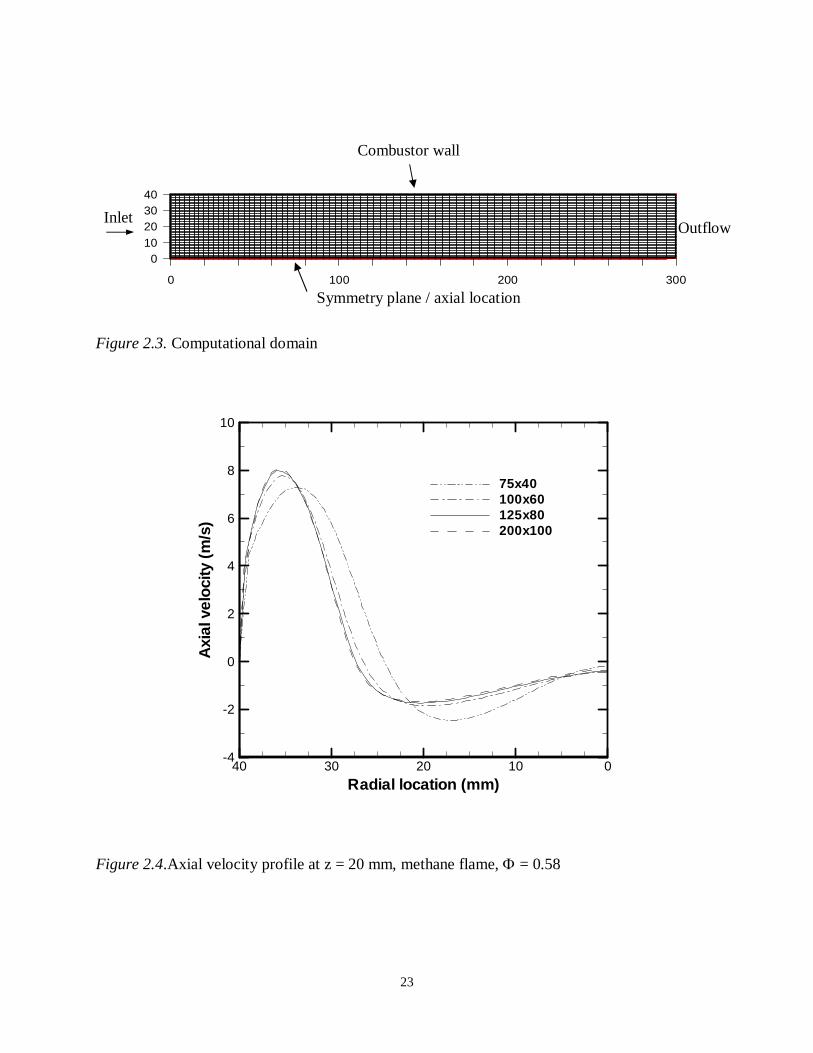
Computations were performed using four different grid sizes: 75 x 40, 100 x 60, 125 x 80
and 200 x 100. Figure 2.4 shows axial velocity profiles at the axial location of 20 mm for
different grid sizes for reacting flow case with Ф = 0.58. Since the results of 125 x 80 and 200 x
100 grids are nearly identical, 125 x 80 grid was used for all calculations to provide grid
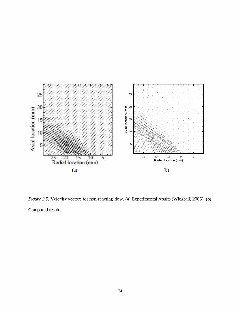
independent solution. Figure 2.5 shows the computed and experimental (Wicksall, 2005) velocity
vectors for non-reacting flow with no porous media. Results show qualitative agreement between
computed and experimental velocity fields. Corner and central recirculation zones are seen in the
vector plots. Inlet flow enters approximately at 35° angle from the vertical, then turns
approximately an additional 10° as flow from the central recirculation zone re-attaches with the
inlet flow. Central and corner recirculation flows re-attach at similar locations for computed and
experimental results. Although simplifying assumptions were made in the computational model,
results qualitatively predict the main features of the flow.
Figure 2.6 shows the computed and experimental (Wicksall, 2005) velocity vectors for
combustion of methane at Ф = 0.58 without porous media. Similar to non-reacting flow,
computed and experimental results show qualitative agreement. Velocities are higher for reacting
case, as expected, due to decrease in density of the products. Main features of the measured flow
are replicated by computations: inlet flow at approximately 35° angle from the vertical,
additional 10° turning as central recirculation zone re-attaches; central and corner recirculation
zones with similar re-attachment locations.

16
2.3 Results and Discussion
Computations were performed for non-reacting and reacting flows. Methane flames of Ф
= 0.58 and 0.85 were modeled for the reacting flow. For each case, effect of PIM on the flow
structure was investigated. Comparison of computed and experimental results is presented.
Results include velocity vectors and radial profiles at different axial locations. Results for non-
reacting and reacting flows are presented in the following sections.
2.3.1 Non-reacting Flow
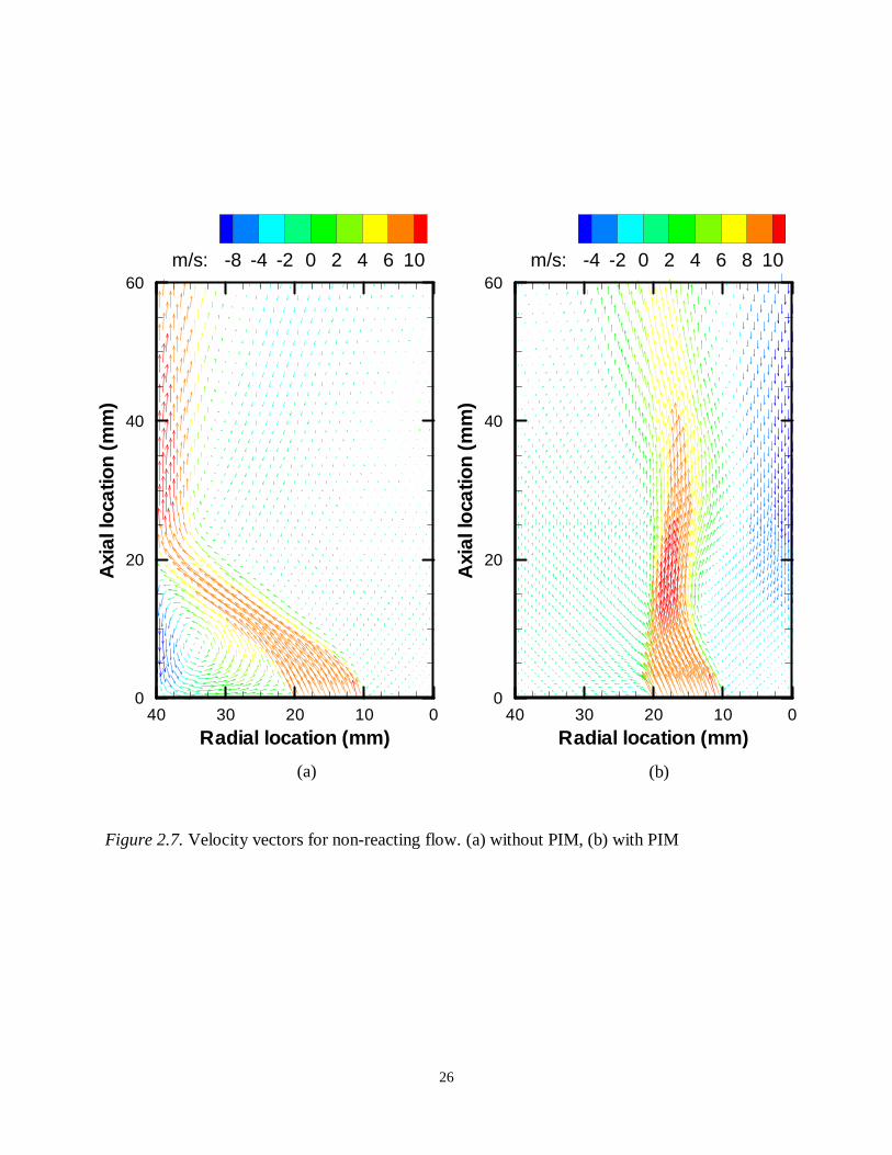
Figure 2.7 shows the computed velocity field in a 40 mm by 60 mm window. Flow
structures with no porous material and with porous material are presented for identical conditions
in Figures 2.7(a) and 2.7(b), respectively. Central and corner recirculation zones are present in
case of the flow field with no porous media. The corner recirculation zone results from the
sudden cross-sectional area expansion in the flow direction. Central recirculation zone extends
across much of the width of the domain. Larger flow velocities occur near the wall of the
enclosure. Presence of PIM in the enclosure dramatically changes the flow structure, as seen in
Figure 2.7(b). Corner recirculation zone disappears because flow is distributed within PIM.
Resistance to the flow introduced by PIM causes inlet flow to tilt vertically. Central recirculation
zone is narrow and more intense compared to its no PIM counterpart.
Next, Figure 2.8 shows axial velocity profiles at different axial locations (z) of the
domain to examine the evolution of the flow without and with PIM. Figure 2.8 shows different
locations of peak axial velocity for flow without and with PIM. Axial velocity peak without PIM
progresses toward the wall and becomes narrow at z = 30 mm. Near the wall, axial velocity is
negative indicating the corner recirculation zone. When PIM is present, axial velocity in the

17
porous region is positive but close to zero, indicating blockage of the flow created by the porous
insert. There is no evidence of a corner recirculation zone. Outside the porous region, axial
velocity peaks at around r = 16 mm. This peak location remains constant as the flow evolves in
the axial direction. Axial velocity near the center has a larger negative value, indicating a more
intense central recirculation zone compared to that without PIM.
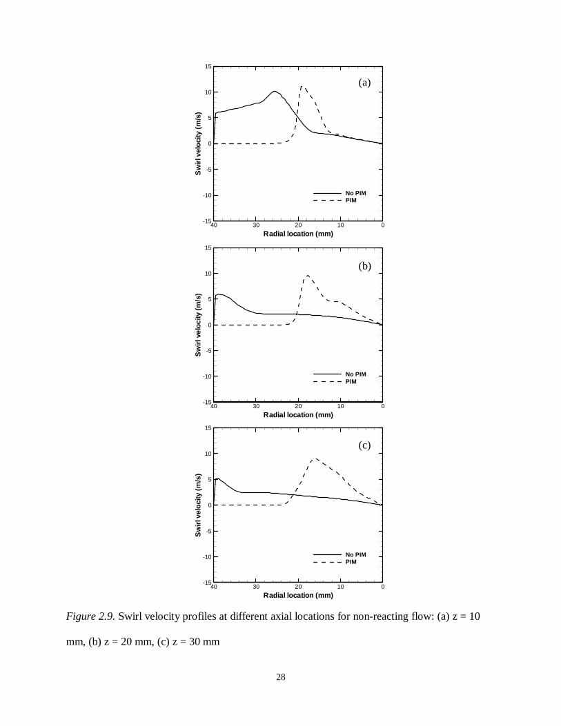
Figure 2.9 shows the evolution of the swirl velocity without and with PIM. Without the
PIM, the location of peak swirl velocity progresses towards the combustor wall, similar to the
peak axial velocity. The peak value of the swirl velocity decreases in the axial direction. When
PIM is present, swirl velocity inside porous region is zero. Outside porous region, swirl velocity
remains approximately constant. Location of peak of swirl velocity remains constant at
approximately r = 16 mm, similar to the axial velocity. These results indicate that the PIM
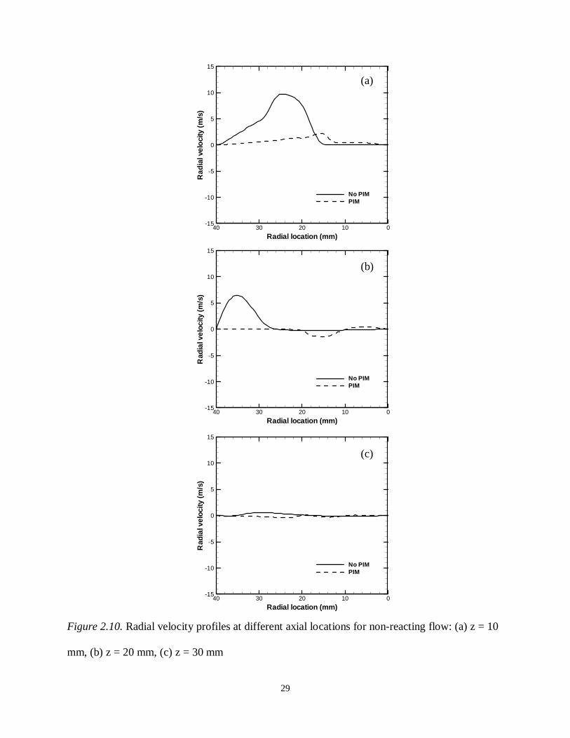
produces a stronger swirl near the center region. Figure 2.10 compares the radial velocity profiles
without and with PIM. Without PIM, peak radial velocity decreases in the axial direction, and its
location progressively shifts towards the combustor wall. At z = 30 mm the radial velocity is
nearly zero. With PIM, the radial component of velocity is nearly zero at all axial locations.
Overall, results indicate that swirling effect induced by the swirl injector is intensified by the
porous insert. Furthermore, the corner recirculation zone is diminished and central recirculation
zone is also intensified.
2.3.2 Reacting Flow
Figure 2.11 shows computed velocity fields in a 40 mm by 60 mm window for reacting
flow without and with PIM. These results show the change in time-averaged flowfield caused by
PIM in the reaction zone. Similar to the non-reacting case, a corner recirculation zone exists

18
without porous insert, as seen in Figure 2.11(a). The central recirculation zone occupies a large
portion of the combustor width. Both corner and central recirculation zones provide a mechanism
for flame stabilization as hot products come in contact with incoming reactant flow, igniting the
mixture to sustain the flame. For case with PIM, Figure 2.11(b), corner recirculation zone is
eliminated by flow redistribution in the porous region. Central recirculation zone becomes more
intense. Presence of PIM changes the flow structure, although typical swirl-stabilization
mechanism is still present. A more intense central recirculation zone remains responsible for
igniting fresh reactant flow in the central region. Although the typical swirl-stabilization
mechanism is affected, the combined swirl-PIM system is also effective in stabilizing the flame.
This remark is consistent with experimental observations showing a stable flame.
Figure 2.12 shows axial velocity profiles at different axial location for reacting flow at Ф
= 0.58. Results indicate trends similar to those obtained for non-reacting flow. Figure 2.12 shows
the axial velocity without and with PIM. Without PIM, the axial velocity peak progresses
towards the wall where a section of negative axial velocity exists, indicating corner recirculation
zone. Presence of PIM causes the axial velocity peak to remain at nearly a constant radial
location. The axial velocity within the porous region is nearly zero. A region of negative axial
velocity with magnitude greater than the no PIM case evolves near the center of the combustor.
PIM restricts the radial extent of the flow recirculation region, which is stronger for the case with
PIM. Figure 2.13 shows the swirl component of the velocity for cases without and with PIM.
With no PIM, swirl velocity of similar magnitude extends across the radial direction. With PIM,
the peak swirl velocity is higher, and it remains approximately constant in the axial direction,
both in magnitude and location. Swirl velocity in the porous region is zero. Similar to the non-
reacting case, swirl effect does not diminish with the presence of PIM. Figure 2.14 shows the

19
radial velocity profiles without and with PIM. Without PIM, radial velocity decreases rapidly in
the axial direction. With PIM, radial velocity is approximately zero at all axial locations.
Reacting flow computations were also performed for Ф = 0.85. Figure 2.15 shows
velocity vectors in the combustion chamber. Results are similar to those for Ф = 0.58. Figures
2.16 to 2.18 show profiles of axial, swirl and radial velocity at different axial locations. Similar
trends to those obtained for reacting flow at Ф = 0.58 are observed. As expected, velocity
magnitudes in this case are greater because of the higher flame temperature. The overall flow
field without or with PIM is unaffected by an increase in the equivalence ratio.
2.4 Conclusions
Flow field in a LPM swirl-stabilized combustor integrated with porous media was
computed. Non-reacting flow and reacting flow were modeled without and with PIM. Flow
resistance associated with PIM was modeled by adding sink terms to the momentum
conservation equations. The sink term was modeled by a power law correlation with coefficients
determined experimentally. Methane flames were modeled for Ф = 0.58 and 0.85. Turbulence
was modeled using the RNG k – ε model. Inlet boundary conditions were simplified assumptions
based on experimental data. Combustion was modeled using a turbulent premixed combustion
model. The computed flow field was compared with experimentally obtained data for reacting
and non-reacting flows. Results show qualitative agreement for both reacting and non-reacting
flows. Change in the flow structure introduced by the porous insert was investigated next.
Results show that the porous insert significantly alters the flow structure. Porous insert
eliminates the corner recirculation zone, vertically orients the gaseous flame zone, intensifies the
central recirculation zone, maintains the swirling effect imparted by the swirl injector, and

20
creates a more uniform flow distribution at downstream locations. These unique features of the
present concept can improve the noise and instability performance of combustor as discussed
next. The flow field is similar for non-reacting and reacting cases, and it is not affected
significantly by an increase in the equivalence ratio.

21
Figure 2.1. Schematic diagram of swirl stabilization mechanism
Swirler
Central recirculation zone
Corner recirculation zone
Flame
Reactants
Combustor wall
Products
Dump plane

22
Figure 2.2. Schematic of combustor with the swirler
8.1
Dimensions in cm
Inlet Swirler
30.6
4.0
23
Figure 2.3. Computational domain
Figure 2.4.Axial velocity profile at z = 20 mm, methane flame, Φ = 0.58
0 100 200 300
010203040
Inlet Outflow
Symmetry plane / axial location
Radial location (mm)
Axi
alve
loci
ty(m
/s)
40 30 20 10 0-4
-2
0
2
4
6
8
10
75x40100x60125x80200x100
Combustor wall
24
Figure 2.5. Velocity vectors for non-reacting flow. (a) Experimental results (Wicksall, 2005), (b)
Computed results
Radial location (mm)
Axi
allo
catio
n(m
m)
25 20 15 10 5
5
10
15
20
25
(a) (b)

25
Figure 2.6. Velocity vectors for reacting flow. (a) Experimental results (Wicksall, 2005), (b)
Computed results
Radial location (mm)
Axi
allo
catio
n(m
m)
25 20 15 10 5
5
10
15
20
25
(a) (b)
26
Figure 2.7. Velocity vectors for non-reacting flow. (a) without PIM, (b) with PIM
(a) (b)
Radial location (mm)
Axi
allo
catio
n(m
m)
40 30 20 10 00
20
40
60m/s: -4 -2 0 2 4 6 8 10
Radial location (mm)
Axi
allo
catio
n(m
m)
40 30 20 10 00
20
40
60m/s: -8 -4 -2 0 2 4 6 10

27
Figure 2.8. Axial velocity profiles at different axial locations for non-reacting flow: (a) z = 10
mm, (b) z = 20 mm, (c) z = 30 mm
Radial location (mm)
Axi
alve
loci
ty(m
/s)
40 30 20 10 0-15
-10
-5
0
5
10
15
No PIMPIM
Radial location (mm)
Axi
alve
loci
ty(m
/s)
40 30 20 10 0-15
-10
-5
0
5
10
15
No PIMPIM
Radial location (mm)
Axi
alve
loci
ty(m
/s)
40 30 20 10 0-15
-10
-5
0
5
10
15
No PIMPIM
(a)
(b)
(c)
28
Figure 2.9. Swirl velocity profiles at different axial locations for non-reacting flow: (a) z = 10
mm, (b) z = 20 mm, (c) z = 30 mm
Radial location (mm)
Sw
irlv
elo
city
(m/s
)
40 30 20 10 0-15
-10
-5
0
5
10
15
No PIMPIM
Radial location (mm)
Sw
irlve
loci
ty(m
/s)
40 30 20 10 0-15
-10
-5
0
5
10
15
No PIMPIM
Radial location (mm)
Sw
irlv
elo
city
(m/s
)
40 30 20 10 0-15
-10
-5
0
5
10
15
No PIMPIM
(a)
(b)
(c)
29
Figure 2.10. Radial velocity profiles at different axial locations for non-reacting flow: (a) z = 10
mm, (b) z = 20 mm, (c) z = 30 mm
Radial location (mm)
Rad
ialv
elo
city
(m/s
)
40 30 20 10 0-15
-10
-5
0
5
10
15
No PIMPIM
Radial location (mm)
Rad
ialv
eloc
ity(m
/s)
40 30 20 10 0-15
-10
-5
0
5
10
15
No PIMPIM
Radial location (mm)
Rad
ialv
eloc
ity(m
/s)
40 30 20 10 0-15
-10
-5
0
5
10
15
No PIMPIM
(a)
(b)
(c)

30
Figure 2.11. Velocity vectors for reacting flow Ф = 0.58. (a) without PIM, (b) with PIM
(a) (b) Radial location (mm)
Axi
allo
catio
n(m
m)
40 30 20 10 0
20
40
60m/s: -8 -6 -2 0 2 6 10 12
Radial location (mm)
Axi
allo
catio
n(m
m)
40 30 20 10 00
20
40
60m/s: -4 -2 0 2 4 6 8 10

31
Figure 2.12.Axial velocity profiles at different axial locations for Ф = 0.58: (a) z = 10 mm, (b) z
= 20 mm, (c) z = 30 mm
Radial location (mm)
Axi
alve
loci
ty(m
/s)
40 30 20 10 0-15
-10
-5
0
5
10
15
No PIMPIM
Radial location (mm)
Axi
alve
loci
ty(m
/s)
40 30 20 10 0-15
-10
-5
0
5
10
15
No PIMPIM
Radial location (mm)
Axi
alve
loci
ty(m
/s)
40 30 20 10 0-15
-10
-5
0
5
10
15
No PIMPIM
(a)
(c)
(b)

32
Figure 2.13. Swirl velocity profiles at different axial locations for Ф = 0.58: (a) z = 10 mm, (b) z
= 20 mm, (c) z = 30 mm
Radial location (mm)
Sw
irlve
loci
ty(m
/s)
40 30 20 10 0-15
-10
-5
0
5
10
15
No PIMPIM
Radial location (mm)
Sw
irlve
loci
ty(m
/s)
40 30 20 10 0-15
-10
-5
0
5
10
15
No PIMPIM
Radial location (mm)
Sw
irlv
elo
city
(m/s
)
40 30 20 10 0-15
-10
-5
0
5
10
15
No PIMPIM
(a)
(c)
(b)

33
Figure 2.14. Radial velocity profiles at different axial locations for Ф = 0.58: (a) z = 10 mm, (b)
z = 20 mm, (c) z = 30 mm
Radial location (mm)
Rad
ialv
elo
city
(m/s
)
40 30 20 10 0-15
-10
-5
0
5
10
15
No PIMPIM
Radial location (mm)
Rad
ialv
elo
city
(m/s
)
40 30 20 10 0-15
-10
-5
0
5
10
15
No PIMPIM
Radial location (mm)
Rad
ialv
eloc
ity(m
/s)
40 30 20 10 0-15
-10
-5
0
5
10
15
No PIMPIM
(a)
(c)
(b)
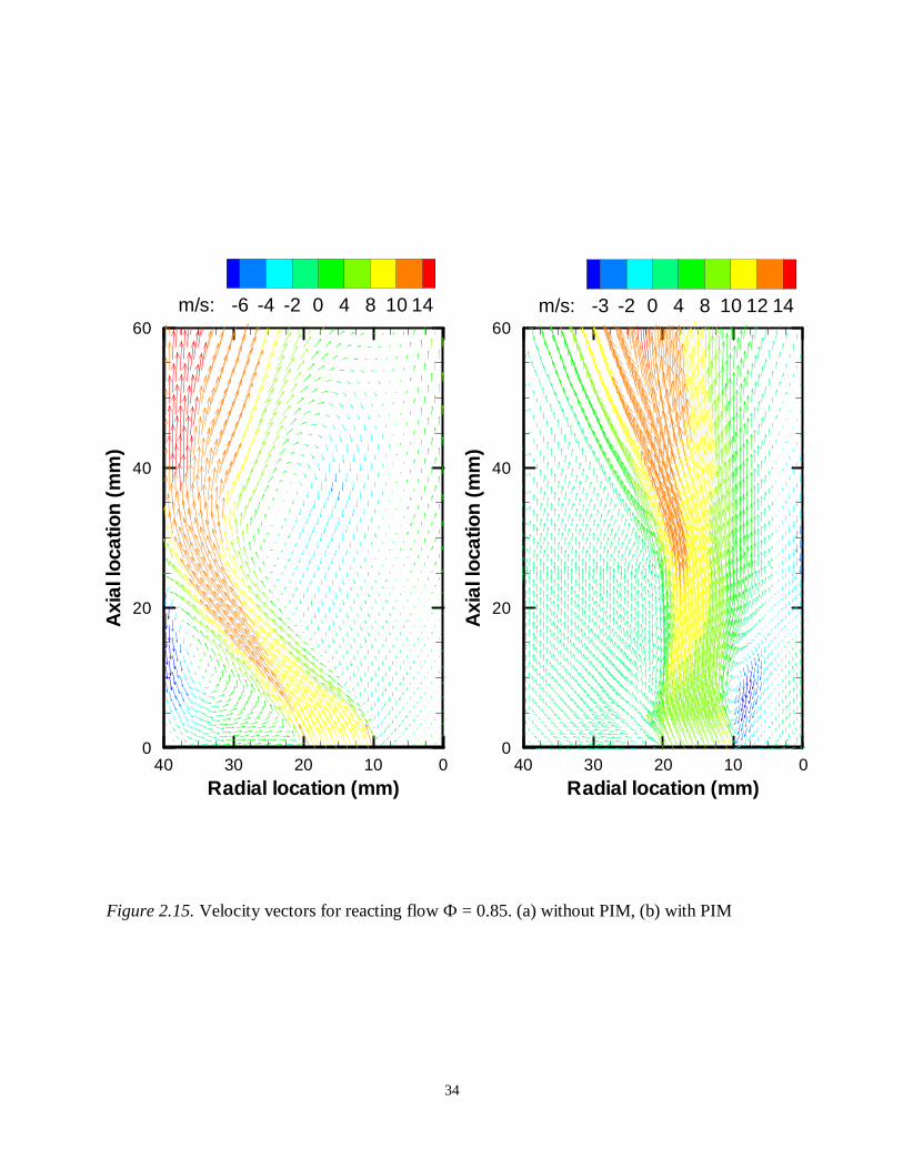
34
Figure 2.15. Velocity vectors for reacting flow Ф = 0.85. (a) without PIM, (b) with PIM
Radial location (mm)
Axi
allo
catio
n(m
m)
40 30 20 10 00
20
40
60
Radial location (mm)
Axi
allo
catio
n(m
m)
40 30 20 10 00
20
40
60m/s: -6 -4 -2 0 4 8 10 14 m/s: -3 -2 0 4 8 10 12 14

35
Figure 2.16. Axial velocity profiles at different axial locations for Ф = 0.85: (a) z = 10 mm, (b) z
= 20 mm, (c) z = 30 mm
Radial position (mm)
Axi
alve
loci
ty(m
/s)
40 30 20 10 0-15
-10
-5
0
5
10
15
PIMNo PIM
Radial position (mm)
Axi
alve
loci
ty(m
/s)
40 30 20 10 0-15
-10
-5
0
5
10
15
PIMNo PIM
Radial position (mm)
Axi
alve
loci
ty(m
/s)
40 30 20 10 0-15
-10
-5
0
5
10
15
PIMNo PIM
(a)
(c)
(b)

36
Figure 2.17. Swirl velocity profiles at different axial locations for Ф = 0.85: (a) z = 10 mm, (b) z
= 20 mm, (c) z = 30 mm
Radial location (mm)
Sw
irlve
loci
ty(m
/s)
40 30 20 10 0-15
-10
-5
0
5
10
15
No PIMPIM
Radial location (mm)
Sw
irlv
elo
city
(m/s
)
40 30 20 10 0-15
-10
-5
0
5
10
15
No PIMPIM
Radial location (mm)
Sw
irlv
elo
city
(m/s
)
40 30 20 10 0-15
-10
-5
0
5
10
15
No PIMPIM
(a)
(c)
(b)
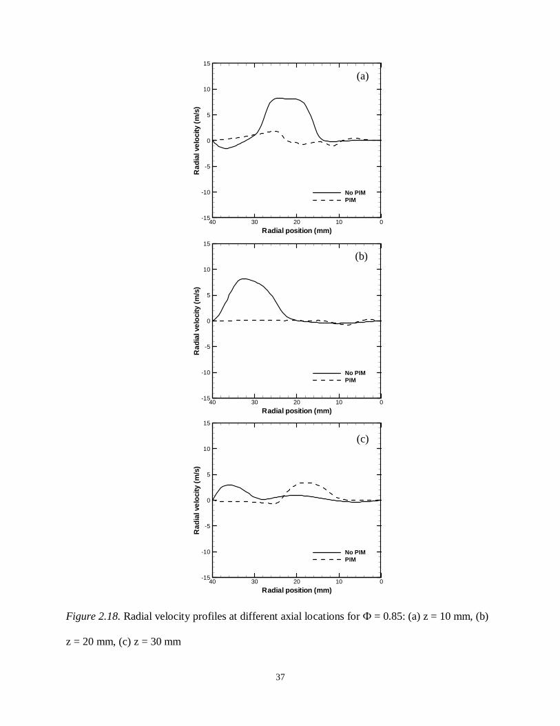
37
Figure 2.18. Radial velocity profiles at different axial locations for Ф = 0.85: (a) z = 10 mm, (b)
z = 20 mm, (c) z = 30 mm
Radial position (mm)
Rad
ialv
elo
city
(m/s
)
40 30 20 10 0-15
-10
-5
0
5
10
15
No PIMPIM
Radial position (mm)
Rad
ialv
elo
city
(m/s
)
40 30 20 10 0-15
-10
-5
0
5
10
15
No PIMPIM
Radial position (mm)
Rad
ialv
elo
city
(m/s
)
40 30 20 10 0-15
-10
-5
0
5
10
15
No PIMPIM
(a)
(c)
(b)

38
CHAPTER 3
NOISE REDUCTION IN SWIRL-STABILIZED COMBUSTOR COUPLED WITH PIM
Background
In recent years, noise emission has become increasingly important to industry and
society. The combustion process is a common source of noise production in gas turbines,
internal combustion engines, industrial burners, and commercial furnaces. Heat release in the
reacting mixture causes dilatation, which produces pressure pulsations that propagate outside the
flame zone as sound waves. Most practical combustion systems operate with the working fluid
in turbulent motion with embedded reaction zones, which alter the noise production mechanism.
In addition to the direct noise produced in the reaction zone, thermal non-uniformities arising
from the combustor can generate indirect noise in downstream components. The topic of this
study is the direct combustion noise, which is often the dominant component of the total sound
power.
The early research on combustion noise is summarized by Putnum (1976) and Strahle
(1978), who report analytical models and empirical data base for sound power level as a function
of burner geometry, flow rate, fuel type, equivalence ratio, etc. In recent years, the research
focus has shifted to LPM combustion systems, driven by the need to comply with the
increasingly stringent emissions regulations. However, typical LPM combustion systems are
prone not only to combustion noise but also to combustion instability characterized by coherent,
fixed frequency feedback oscillations. Combustion noise and instability are distinct outcomes,

39
yet they both arise from the same source, i.e., heat release fluctuations in a turbulent flow with
multiple length and time scales. In recent years, several experimental and computational studies
have helped in the understanding of the noise generation mechanisms (Schwarz, 2009; Rajaram,
2006; Flemming, 2005; Choi, 2005; Hirsch, 2007; Tiribuzi, 2008; Duchaine, 2009; Lieuwen,
2005; Lee, 2003; Richards, 2003; Noiray, 2009). In particular, the advent of computational fluid
dynamics (CFD) has afforded the opportunity to analyze noise generation mechanism by
incorporating detailed physics of turbulent combustion with the acoustics. These studies have
identified passive and active methods to control combustion noise and instabilities.
The effectiveness of an active combustion control system depends upon actuation,
sensing, and control algorithms, among other factors. In spite of the significant progress in these
areas, complete reliability of active combustion control is still a major concern since an
unexpected event can destroy the system within a fraction of second. Thus, in this study, a
passive technique involving the use of PIM to suppress combustion noise and/or instability is
investigated. The PIM is an open-cell foam structure alloyed with HfC/SiC to protect the foam
material from high temperature oxidation by creating refractory surface oxides that offer
nominally 600°C higher use temperature than SiC alone. The vortex shedding mechanism of
combustion noise and/or instability is curtailed on source by inserting a properly designed porous
structure to constrain the recirculation regions in the swirl-stabilized combustor. The porous
structure is intended to limit and/or disintegrate vortical structures in the flame to produce a more
homogeneous flow field with limited regions of flow reversal. Previous experiments revealed
that introducing a porous insert is a promising concept for further investigation (Agrawal, 2008).
In this chapter, the experimental set up to acquire noise and pollutant emissions data for a range

40
of geometric and operating conditions is described. Then, results and discussions are presented
followed by the conclusions of the study.
3.2 Experimental Setup
The test apparatus is shown schematically in Figure 3.1. The combustion chamber
operated at atmospheric pressure is a 30.0 cm long, 8.0 cm ID quartz cylinder to enclose to
flame. Heated air enters the system through a plenum filled with marbles to breakdown the large
vortical structures. The air passes through a swirler into the mixing section, where the gaseous
methane is supplied. Air and fuel premix in the mixing region before entering the dump plane of
the combustion chamber through a swirler. The swirler has six vanes positioned at 28o to the
horizontal, and it results in theoretical swirl number of 1.5 (see Appendix B for calculation). The
inlet Reynolds number based on the equivalent diameter ranged from 5,000 to 10,000. The
combustor is back-side cooled by natural convection. A compressed storage tank supplies air
that passes through a pressure regulator, water traps, flow control valve, and an in-line electrical
heater before reaching the experiment. Methane fuel is also supplied from a rack of storage
tanks. Air flow rate is measured by a laminar flow elements (LFE) calibrated for 0 to 1000 liters
per minute (lpm) of air. The LFE for fuel flow rate measurements is calibrated for 0 to 100 lpm
of methane. The flow rate measured by the LFE is corrected for temperature and pressure as
specified by the manufacturer.
Sound pressure data are collected using a Brüel & Kjær microphone probe (Model 4189)
located 28 cm from the edge of the combustor exit plane. A total number of 10000 samples are
acquired in 5 sec at 2000 Hz. The measured voltage signal is converted to pressure fluctuation
data using the probe sensitivity of 44.3 mV/Pa. An FFT analysis is performed to obtain the
41
power spectrum. A Matlab script was written to compute the sound pressure level (SPL) in
decibels (dB) given as (Bussman, 2001):
�.� = 10 ∗ log� �.����.���� � (3.1)
Where Pref = 20 µPa. Total SPL was calculated by:
�.������ = 10 ∗ log� /�10.�∗� !����� 0 (3.2)
Where SPLi is the SPL at each frequency level, n is the number of frequency bands. One-third
octave frequency bands were used, from bands 13 to 29, with centers at 20 Hz and 800 Hz
respectively (Bussman, 2001).
Emissions measurements are taken by continuously sampling the product gas by a quartz
probe (OD = 7.0 mm) attached to a three-way manual traversing system. The upstream tip of the
probe was tapered to 1 mm ID to quench reactions inside the probe. The gas sample passed
through an ice bath and water traps to remove moisture upstream of the gas analyzers. The dry
sample passed through electrochemical analyzers to measure the concentrations of CO and NOx
in ppm. The analyzer also measures oxygen and carbon dioxide concentrations, which are used
to cross-check the equivalence ratio obtained from the measured fuel and air flow rates. The
uncorrected emissions data on dry basis are reported with measurement uncertainty of ±2 ppm.

42
3.3 Results and Discussion
In this study, porous inserts of different pore sizes and inside diameters were used. Figure
3.2 shows a photograph of a PIM insert and photographs of the combustor without and with the
PIM insert. Figure 3.3 shows diagrams of the PIM inserts configurations used in this study. All
inserts were 2.5 cm thick, 8.0 cm OD, and had porosity of 85%. The inside diameters were 3.8
cm, 4.4 cm and 5.0 cm, and the pore densities were 4 pores per cm (ppcm), 8 ppcm, and 18
ppcm. For each experiment, two pieces of PIM were stacked together labeled, for example, as
D38-P4 + D44-P4. This configuration pertains to a PIM piece with 3.8 cm inside diameter and
pore density of 4 ppcm followed by (in the direction of the flow) another PIM piece with 4.4 cm
inside diameter and pore density of 4 ppcm. Experiments were conducted at equivalence ratios
(Ф) of 0.7 and 0.8 with airflow rate (Q) of (1) 300 slpm at inlet temperature (Ti) of 100˚C, and
(2) 600 slpm at inlet temperature of 120˚C.
Figure 3.4 shows flames images for Ф=0.7, Q=300 slpm, and Ti=100˚C. Without the
porous insert, the image in Figure 3.4(a) depicts a blue flame typical of LPM combustion. The
image in Figure 3.4(b) pertains to configuration D38-P4+D44-P4. The orange glow in this
image indicates combustion stabilized within the PIM. A confined blue gaseous flame is also
visible (though barely) downstream of the PIM. The image in Figure 3.4(c) reveals a
fundamentally different combustion mode for configuration D38-P18+D38-P18; small blue
flamelets are stabilized on the surface of the porous insert while majority of the reactants burn in
the confined, swirl-stabilized gaseous flame region. The interior combustion mode for the
configuration in Figure 3.4(b) is detrimental for material strength, and it also produced higher
sound pressure levels.

43
Porous insert in the combustor alters the flow field and flame structure by restricting and
re-directing reactants and products inside the combustion chamber. Elimination of the corner
recirculation zone also fundamentally changes the stabilization mechanism of the flame.
Reactant flow exiting the swirl injector is divided into the center (core) region and PIM region.
The reactant flow rate in the PIM would depend upon the flow resistance offered by the PIM.
The reactant flow in the center region results in the typical swirl-stabilized flame, albeit of higher
swirl intensity because of the constrained volume of the free flame. Combustion products from
the free flame would enter the porous insert through the inner surface and mix with the reactants
introduced upstream, as illustrated in Figure 3.5. Combustion products would also transfer heat
to the porous insert, and further to the reactants flowing through the PIM, which leads to interior
or surface combustion depending upon the resulting flame speed and porous insert geometry.
This fundamental mechanism is the basis for all cases studied with PIM inserts. Interior
combustion occurs when the reactants ignite and sustain a flame within the PIM. In this case, a
balance is achieved between: (1) energy of unburned reactants flowing in the PIM, (2) energy of
products from the free flame penetrating the PIM, and (3) heat transfer between free flame and
the PIM. This balance can be expected to depend upon the PIM pore density, PIM geometry,
reactants velocity. Surface combustion occurs if reactants do not ignite within the PIM. Instead,
the flame is established on the downstream surface of the PIM.
Interior and surface combustion modes excite the acoustic field differently, thus resulting
in different noise levels. Interior combustion is accompanied with intense thermal radiation from
the PIM, and it generally produced higher noise levels. The surface combustion produced blue
flamelets similar to the free flame, and this mode of combustion generally mitigated the noise
produced in the free flame without the porous insert. Surface combustion mode is hypothesized

44
to reduce the noise levels for the following reasons: (1) the heat release rate in the free flame is
reduced because some of the reactants also burn downstream of the PIM surface as a distributed
flame, (2) PIM suppresses the pressure fluctuations in the adjacent free flame, and (3) the
vortical structures produced in the corner recirculation zone and shear regions are virtually
eliminated.
3.3.1 Effect of PIM Pore Density
Figure 3.6 shows five data sets for Q = 300 slpm, no PIM and Ф = 0.7. These data were
taken independently to demonstrate repeatability of noise measurements. Sound pressure levels
overlap one another, indicating measurements are repeatable. Table 3.1 presents a summary of
total SPL measured for the baseline case (no PIM) and each configuration with PIM. Results are
presented at Φ = 0.7 and 0.8. Each result presented is the average of 5 independent
measurements. Figure 3.7 shows flame images for Q = 300 slpm at Ф = 0.7 for baseline case
without and with PIM. Figure 3.8 shows flame images for Q = 300 slpm at Ф = 0.8. Porous insert
of 4 ppcm resulted in interior combustion for both Φ (Figures 3.7(b) and 3.8(b)). Compared to
baseline case, total SPL decreased by 2.9 dB for Φ = 0.7, and increased by 3.2 dB for Φ = 0.8.
Porous insert of 8 ppcm also resulted in interior combustion for both Φ (Figures 3.7(c) and
3.8(c)). For Φ = 0.7, the total SPL decreased by 6.8 dB. For Φ = 0.8, noise level increased by 1.0
dB. Porous insert of 18 ppcm resulted in surface combustion for Φ = 0.7 and reduction in total
SPL by 7.1 dB. For Φ = 0.8, interior combustion was confined to a narrow downstream region of
the PIM insert (Figure 3.8(d)) and the total SPL decreased by 4.0 dB. Results show that the
highest pore density of 18 ppcm is most effective in mitigating the combustion noise. Note that

45
this case resulted in surface combustion (or interior combustion in a narrow downstream region).
Thus, achieving PIM surface combustion mode is important to reduce the total SPLs.
Figure 3.9 presents the power spectra for all configuration at Ф = 0.7. Figures 3.9(a),
3.9(b) and 3.9(g) show a peak at a frequency of about 250 Hz typical of combustion instability.
These cases pertain to the highest SPLs. For the remaining cases, the power spectra are
broadband with no distinct peak, thus, combustion instability without PIM was mitigated by
PIM. Figure 3.10 shows power spectra for all configurations at Φ = 0.8. Figure 3.10(b) shows a
peak at frequency of 450 Hz, and Figures 3.10(c) and 3.10(h) show peaks at frequency of 700
Hz. Figures 3.10(d) and 3.10(g) show peaks at approximately 250 Hz, and power spectra in
Figures 3.10 (e) and 3.10(f) are broadband. Figure 3.11 shows SPL in one third octave band for
all PIM configurations. Results show that the pore density of 18 ppcm is most effective in
mitigating the combustion noise at higher frequencies.
Table 3.1
Summary of results, effect of pore density, Q = 300 slpm
Configuration PIM Ф = 0.7 Ф = 0.8 Pore density
(ppcm)
A None 103.0 dB 103.9 dB N/A
B D38-P4 + D44-P4 100.1 dB 107.1 dB 4
C D38-P8 + D44-P8 96.2 dB 104.9 dB 8
D D38-P18 + D44-P18 95.4 dB 99.8 dB 18

46
3.3.2 Effect of PIM Geometry
By changing PIM dimensions with a fixed pore density, the flow structure can be affected
to favor or avoid the interior combustion. Thus, PIM geometry can be expected to affect the total
SPLs. Experiments were conducted with 18 ppcm porous inserts of different inside diameters.
The PIM geometries studied are: constant, increasing, and decreasing inside diameter in the flow
direction. Table 3.2 lists all cases studied and a summary of the total SPLs.
Figure 3.12 shows the SPL in one third octave band for Q = 300 slpm and different PIM
geometries. PIM configurations D, E and F resulted in very similar total SPLs; 6.0 dB reduction
at Φ = 0.7, and 4.0 dB reduction at Φ = 0.8 compared to the baseline case with no PIM. Note that
these cases had no indication of interior combustion. For these cases, the inside diameter (3.8
cm) of the upstream porous insert is the same as the outside diameter of the swirl injector at the
dump plane. Similar to Configuration F, the Configuration G uses constant inside diameter
porous rings. However, the total SPL decreased only by 2.2 dB at Φ = 0.7 and increased by 1.9
dB at Φ = 0.8. This result is attributed to the increased volume of the free flame region, which
changes the stabilization mechanism by approaching conditions similar to the baseline case, i.e.,
corner recirculation zone accompanied with vortical structures in the shear layer of the flame. In
this case, interior combustion was observed on the inner surface of the porous insert. PIM
configuration H reduced the total SPL by 6.8 dB at Φ = 0.7. However, at Φ = 0.8, the total SPL
increased by 3.9 dB. The downstream confinement of the free flame increases entrainment of
products into the porous insert, which promotes interior combustion mode to increase noise
levels.
47
3.3.3 Effect of Reactant Flow Rate
Experiments were conducted at a higher air flow rate of Q=600 slpm with Ti=120˚C. In
this case, none of the PIM flames at Ф=0.7 experienced interior combustion indicating
sufficiently high flow velocity through the pores. In spite of the high reactant flow rate,
submerged combustion still occurred at Ф = 0.8. However, tests indicate a dramatic reduction in
combustion noise at the higher flow rate. That is, the PIM is very effective in redistributing the
flow in the flame region to suppress heat release fluctuations, for example, originating from the
turbulent vortical structures in the recirculation zones. Figures 3.13 to 3.16 show flame images
for cases with PIM, Q = 300 and 600 slpm at Ф = 0.7 and 0.8. Figure 3.17 shows the power
spectra for configurations A (no PIM), D (divergent), G (constant) and I (convergent) for Q =
600 slpm at Ф = 0.7. Configuration A without PIM shows peaks at frequencies between 350 and
700 Hz. All configurations with PIM resulted in broadband power spectra. Thus, dominant peaks
present without PIM were mitigated with all PIM geometries. Figure 3.18 shows power spectra
for Q = 600 slpm at Ф = 0.8. Several peaks occur without the PIM (Figure 3.18(a)), which is an
indication of combustion instabilities. Figure 3.18(b) shows that the spectral peaks are virtually
eliminated with the use of divergent PIM in the combustor. Total SPL at this high flow rate are
also summarized in Table 3.3.
Figure 3.19 shows SPL in one third octave band for Q = 300 slpm, Ф = 0.7 and 0.8.
Figure 3.20 shows SPL in one third octave band for Q = 600 slpm, Ф = 0.7 and 0.8. For Ф=0.7,
all porous inserts were effective in reducing the noise/instability, with typical reductions in total
SPL of 13 to 14 dB, particularly at higher frequencies. At the higher equivalence ratio, only the
divergent configuration was effective in reducing the total SPL by 13 dB, also by mitigating
power at higher frequencies. Configurations G (constant) and I (convergent) were either
48
ineffective or marginally effective because of the increased propensity for interior combustion.
These results show that the porous insert can effectively mitigate combustion instabilities when
interior combustion can be avoided.
Table 3.2
Summary of results, effect of geometry, Q = 300 slpm
Configuration PIM Ф = 0.7 Ф = 0.8 Inside wall
A None 103.0 dB 103.9 dB N/A
D D38-P18 + D44-P18 95.4 dB 99.8 dB Divergent
E D38-P18 + D50-P18 95.4 dB 99.9 dB
F D38-P18 + D38-P18 95.7 dB 99.8 dB Constant
G D50-P18 + D50-P18 96.1 dB 104.8 dB
H D50-P18 + D38-P18 96.2 dB 106.8 dB Convergent
I D44-P18 + D38-P18 96.2 dB 106.8 dB
49
Table 3.3
Summary of results, effect of flow rate
Configuration Air Flow Rate 300 slpm 600 slpm
PIM / Ф 0.7 0.8 0.7 0.8
A None 103.0 dB 103.9 dB 118.9 dB 120.5 dB
D D38-P18 + D44-P18 95.4 dB 99.8 dB 105.9 dB 107.1 dB
G D50-P18 + D50-P18 96.1 dB 104.8 dB 104.7 dB 120.4 dB
I D44-P18 + D38-P18 96.2 dB 106.8 dB 105.8 dB 115.1 dB
3.3.4 CO and NOx Emissions
Figures 3.21 and 3.22 present the CO and NOx emissions measured for Q=300 slpm, and
Ti=100˚C at Ф=0.7 and 0.8. For Ф=0.7, the CO concentrations for the divergent configuration
are slightly higher and the NOx emissions are comparable for all configurations. For Ф=0.8, all
cases result in comparable CO emissions, but NOx emissions are the highest for the constant area
insert. Interestingly, the NOx emissions for the divergent PIM are comparable to the case
without PIM. For all cases, emissions profiles are nearly flat in the radial direction, indicating
good spatial uniformity of combustion. Overall, results show that the porous insert does not
have an adverse effect on CO and NOx emissions.
Figures 3.23 and 3.24 show the CO and NOx emissions measured at the combustor exit
plane for Q = 600 slpm, Ti=100˚C at Ф=0.7 and 0.8.. For Ф=0.7, Figure 3.23(a) shows that the
CO emissions without the PIM vary from 25 to 30 ppm. With PIM, the CO emissions decrease

50
significantly to below 10 ppm for all porous inserts. The same trend is also observed at Ф=0.8
(Figure 3.24(a)), where the CO emissions with PIM insert are nearly one-third of those without
the PIM. Figures 3.23(b) and 3.24(b) show that the NOx emissions increase slightly with the
PIM insert. Overall, the results are very encouraging and suggest that significant reductions in
noise and pollutant emissions are feasible by a judicial choice of PIM configuration.
3.3.5 Long Duration Experiments
To ensure durability of the porous material used in this investigation, a long-duration test
was conducted, simulating a realistic gas turbine scenario. Test was run continuously during a 4-
hour period. A divergent PIM configuration was used for Q = 600 slpm and Ф = 0.7 because of
promising results obtained in previous section. The objective was to test material endurance over
several hours of operation, to identify damage if any, and its effect on noise, CO and NOx
emissions. Every 30 minutes, CO and NOx emissions data were collected at the center point of
the exit plane and noise data were collected at the combustor exit plane. Results show a steady
flame throughout the duration of the test as reflected by SPL and emissions data. Figure 3.25
shows a plot of SPL in one third octave band taken at 30 minute intervals. Profiles nearly overlap
with each other, indicating no major changes during the experiment. Table 3.4 summarizes the
total SPL throughout the test, and shows that it is nearly constant. Figure 3.26 shows CO and
NOx emissions measured at 30 minute intervals. CO and NOx concentrations are nearly constant
throughout the experiment. Again, these results indicate reliable operation of combustor with
PIM for several hours.

51
Table 3.4
Summary of SPL for long-duration experiment
Time (min) 0 30 60 90 120 150 180 210 240
Total SPL (dB) 106.9 105.7 106.3 105.3 104.2 106.1 105.5 106.1 105.7
3.4 Conclusions
In this study, a novel concept to integrate PIM with swirl-stabilized LPM combustion is
proposed to passively reduce combustion noise. Experimental study shows that the swirl-
stabilized combustion is supplemented with submerged or surface combustion in the presence of
the porous insert. Equivalence ratio, reactant flow rate, and parameters such as PIM pore size and
ID determine the combustion mode. Surface combustion is a desirable mode, while submerged
combustion must be avoided to achieve low SPLs. Results show that a divergent porous insert
with pore density of 18 ppcm can reduce the total SPL by up to 14 dB, depending upon the
reactant flow rate, without adversely affecting the NOx and CO emissions. Furthermore, PIM
insert mitigates combustion instability present without PIM. No noticeable change in noise and
emissions measurements and material properties was observed for long duration tests over a
period of 4 hours. This remarkable performance can be achieved with minimal changes to the
combustor hardware. Thus, the concept presented here is attractive for passive control of
combustion noise and instabilities.

52
Figure3.1. Schematic diagram of experimental setup
Combustion chamber
PIM
Swirler
Premix section
Fuel inlet
Plenum Air inlet
Products
Air heater

53
Figure 3.2. Photos of PIM inserts (a) PIM insert (b) combustor without PIM (c) combustor with
two PIM pieces
(a)
(b) (c)

54
Figure 3.3. Description and schematic diagram of PIM configurations used in this study
Configuration I Pore density: 18 ppcm IDs: 4.4, 3.8 cm
Configuration A Pore density: None IDs: None
Configuration B Pore density: 4 ppcm IDs: 3.8, 4.4 cm
Configuration C Pore density: 8 ppcm IDs: 3.8, 4.4 cm
Configuration H Pore density: 18 ppcm IDs: 5.0, 3.8 cm
Configuration G Pore density: 18 ppcm IDs: 5.0, 5.0 cm
Configuration F Pore density: 18 ppcm IDs: 3.8, 3.8 cm
Configuration E Pore density: 18 ppcm IDs: 3.8, 5.0 cm
Configuration D Pore density: 18 ppcm IDs: 3.8, 4.4 cm
None (Baseline)

55
Figure 3.4. Flame images, (a) without PIM (b) with PIM interior combustion (c) with PIM
surface combustion
(a) (b) (c)

56
Figure 3.5. Schematic diagram illustrating the PIM stabilization mechanism
Surface flame
Reactants
Products
PIM
Swirler
Reactants
Core region flame

57
Figure 3.6. One third octave band SPL for repeatability test
Frequency (Hz)
SP
L(d
B)
0
0
200
200
400
400
600
600
800
800
1000
1000
40 40
60 60
80 80
100 100
120 120
140 140

58
Figure 3.7. Flame images for Q = 300 slpm, Ф = 0.7 (a) Configuration A (b) Configuration B (c)
Configuration C (d) Configuration D (e) Configuration E (f) Configuration F (g) Configuration
G (h) Configuration H (i) Configuration I
(a) (b) (c)
(d) (e) (f)
(g) (h) (i)

59
Figure 3.8. Flame images for Q = 300 slpm, Ф = 0.8 (a) Configuration A (b) Configuration B (c)
Configuration C (d) Configuration D (e) Configuration E (f) Configuration F (g) Configuration
G (h) Configuration H (i) Configuration I
(a) (b) (c)
(d) (e) (f)
(g) (h) (i)

60
Figure 3.9. Power spectra for Q = 300 slpm, Ф = 0.70 (a) Configuration A (b) Configuration B
(c) Configuration C (d) Configuration D (e) Configuration E (f) Configuration F (g)
Configuration G (h) Configuration H (i) Configuration I
(a) (b) (c)
(d) (e) (f)
(g) (h) (i)
Frequency (Hz)
Po
wer
(A.U
.)
0 200 400 600 800 10000
0.1
0.2
0.3
0.4
Frequency (Hz)
Po
wer
(A.U
.)
0 200 400 600 800 10000
0.1
0.2
0.3
0.4
Frequency (Hz)
Po
wer
(A.U
.)
0 200 400 600 800 10000
0.1
0.2
0.3
0.4
Frequency (Hz)
Po
wer
(A.U
.)
0 200 400 600 800 10000
0.1
0.2
0.3
0.4
Frequency (Hz)
Po
wer
(A.U
.)
0 200 400 600 800 10000
0.1
0.2
0.3
0.4
Frequency (Hz)
Po
wer
(A.U
.)
0 200 400 600 800 10000
0.1
0.2
0.3
0.4
Frequency (Hz)
Po
wer
(A.U
.)
0 200 400 600 800 10000
0.1
0.2
0.3
0.4
Frequency (Hz)
Po
wer
(A.U
.)
0 200 400 600 800 10000
0.1
0.2
0.3
0.4
Frequency (Hz)
Po
wer
(A.U
.)
0 200 400 600 800 10000
0.1
0.2
0.3
0.4

61
Figure 3.10. Power spectra for Q = 300 slpm, Ф = 0.80 (a) Configuration A (b) Configuration B
(c) Configuration C (d) Configuration D (e) Configuration E (f) Configuration F (g)
Configuration G (h) Configuration H (i) Configuration I
(a) (b) (c)
(d) (e) (f)
(g) (h) (i)
Frequency (Hz)
Po
wer
(A.U
.)
0 200 400 600 800 10000
0.1
0.2
0.3
0.4
Frequency (Hz)
Po
wer
(A.U
.)
0 200 400 600 800 10000
0.1
0.2
0.3
0.4
Frequency (Hz)
Po
wer
(A.U
.)
0 200 400 600 800 10000
0.1
0.2
0.3
0.4
Frequency (Hz)
Po
wer
(A.U
.)
0 200 400 600 800 10000
0.1
0.2
0.3
0.4
Frequency (Hz)
Po
wer
(A.U
.)
0 200 400 600 800 10000
0.1
0.2
0.3
0.4
Frequency (Hz)
Po
wer
(A.U
.)
0 200 400 600 800 10000
0.1
0.2
0.3
0.4
Frequency (Hz)
Po
wer
(A.U
.)
0 200 400 600 800 10000
0.1
0.2
0.3
0.4
Frequency (Hz)
Po
wer
(A.U
.)
0 200 400 600 800 10000
0.1
0.2
0.3
0.4
Frequency (Hz)
Po
wer
(A.U
.)
0 200 400 600 800 10000
0.1
0.2
0.3
0.4

62
Figure 3.11. One third octave band SPL, effect of pore density, Q = 300 slpm (a) Ф = 0.70 (b) Ф
= 0.8
(a)
(b)
Frequency (Hz)
SP
L(d
B)
0 200 400 600 800 100050
60
70
80
90
100
110
120
130
No PIM4 ppcm8 ppcm18 ppcm
Frequency (Hz)
SP
L(d
B)
0 200 400 600 800 100050
60
70
80
90
100
110
120
130
No PIM4 ppcm8 ppcm18 ppcm

63
Figure 3.12. One third octave band SPL, effect of geometry, Q = 300 slpm (a) Ф = 0.70 (b) Ф =
0.8
Frequency (Hz)
SP
L(d
B)
0 200 400 600 800 100050
60
70
80
90
100
110
120
130
No PIMDivergent 1 (D)Divergent 2 (E)Constant 1 (F)Constant 2 (G)Convergent 1 (H)Convergent 2 (I)
Frequency (Hz)
SP
L(d
B)
0 200 400 600 800 100050
60
70
80
90
100
110
120
130
No PIMDivergent 1 (D)Divergent 2 (E)Constant 1 (F)Constant 2 (G)Convergent 1 (H)Convergent 2 (I)
(a)
(b)
64
Figure 3.13. Flame images for Q = 300 slpm, Ф = 0.7 (a) Configuration A (b) Configuration D
(c) Configuration G (d) Configuration I
(a)
(b)
(c)
(d)

65
Figure 3.14. Flame images for Q = 300 slpm, Ф = 0.8 (a) Configuration A (b) Configuration D
(c) Configuration G (d) Configuration I
(a)
(b)
(c)
(d)

66
Figure 3.15. Flame images for Q = 600 slpm, Ф = 0.7 (a) Configuration A (b) Configuration D
(c) Configuration G (d) Configuration I
(a)
(b)
(c)
(d)

67
Figure 3.16. Flame images for Q = 600 slpm, Ф = 0.8 (a) Configuration A (b) Configuration D
(c) Configuration G (d) Configuration I
(a)
(b)
(c)
(d)
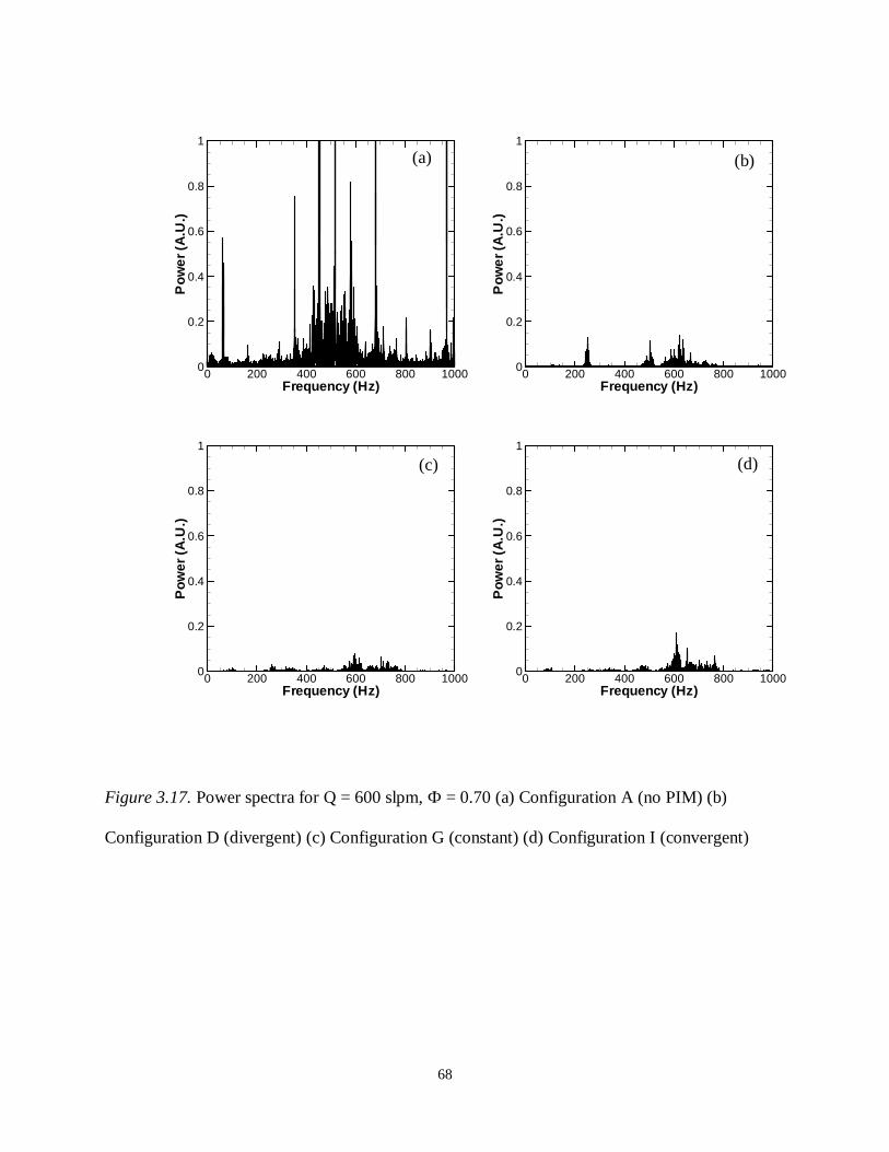
68
Figure 3.17. Power spectra for Q = 600 slpm, Ф = 0.70 (a) Configuration A (no PIM) (b)
Configuration D (divergent) (c) Configuration G (constant) (d) Configuration I (convergent)
(a) (b)
(c) (d)
Frequency (Hz)
Po
we
r(A
.U.)
0 200 400 600 800 10000
0.2
0.4
0.6
0.8
1
Frequency (Hz)
Po
we
r(A
.U.)
0 200 400 600 800 10000
0.2
0.4
0.6
0.8
1
Frequency (Hz)
Po
wer
(A.U
.)
0 200 400 600 800 10000
0.2
0.4
0.6
0.8
1
Frequency (Hz)
Po
wer
(A.U
.)
0 200 400 600 800 10000
0.2
0.4
0.6
0.8
1

69
Figure 3.18. Power spectra for Q = 600 slpm, Ф = 0.80 (a) Configuration A (no PIM) (b)
Configuration D (divergent) (c) Configuration G (constant) (d) Configuration I (convergent)
(a) (b)
(c) (d)
Frequency (Hz)
Po
we
r(A
.U.)
0 200 400 600 800 10000
0.2
0.4
0.6
0.8
1
Frequency (Hz)
Po
we
r(A
.U.)
0 200 400 600 800 10000
0.2
0.4
0.6
0.8
1
Frequency (Hz)
Po
we
r(A
.U.)
0 200 400 600 800 10000
0.2
0.4
0.6
0.8
1
Frequency (Hz)
Po
we
r(A
.U.)
0 200 400 600 800 10000
0.2
0.4
0.6
0.8
1

70
Figure 3.19. One third octave band SPL, effect of reactants flow rate, Q = 300 slpm (a) Ф = 0.7
(b) Ф = 0.8
Frequency (Hz)
SP
L(d
B)
0 200 400 600 800 100050
60
70
80
90
100
110
120
130
No PIMDivergentConstantConvergent
Frequency (Hz)
SP
L(d
B)
0 200 400 600 800 100050
60
70
80
90
100
110
120
130
No PIMDivergentConstantConvergent
(a)
(b)

71
Figure 3.20. One third octave band SPL, effect of reactants flow rate, Q = 600 slpm (a) Ф = 0.7
(b) Ф = 0.8
(a)
(b)
Frequency (Hz)
SP
L(d
B)
0 200 400 600 800 100050
60
70
80
90
100
110
120
130
No PIMDivergentConstantConvergent
Frequency (Hz)
SP
L(d
B)
0 200 400 600 800 100050
60
70
80
90
100
110
120
130
No PIMDivergentConstantConvergent

72
Figure 3.21. CO and NOx emissions for Q = 300 slpm, Ф = 0.7, Ti = 100˚C (a) CO (b) NOx
(a)
(b)
Transverse distance (cm)
CO
(ppm
)
-4 -2 0 2 40
5
10
15
20No PIMDivergentConstantConvergent
Transverse distance (cm)
NO
x(p
pm
)
-4 -2 0 2 40
5
10
15
20
25
No PIMDivergentConstantConvergent

73
Figure 3.22. CO and NOx emissions for Q = 300 slpm, Ф = 0.8, Ti = 100˚C (a) CO (b) NOx
(a)
(b)
Transverse distance (cm)
CO
(pp
m)
-4 -2 0 2 40
5
10
15
20
25
30
No PIMConstantConvergentDivergent
Transverse distance (cm)
NO
x(p
pm
)
-4 -2 0 2 410
20
30
40
50
60
70
No PIMDivergentConstantConvergent
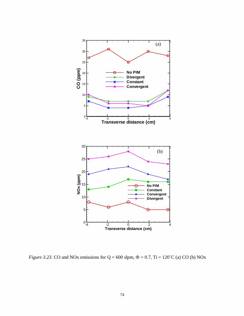
74
Figure 3.23. CO and NOx emissions for Q = 600 slpm, Ф = 0.7, Ti = 120˚C (a) CO (b) NOx
(a)
(b)
Transverse distance (cm)
NO
x(p
pm
)
-4 -2 0 2 40
5
10
15
20
25
30
No PIMConstantConvergentDivergent
Transverse distance (cm)
CO
(ppm
)
-4 -2 0 2 40
5
10
15
20
25
30
35
No PIMDivergentConstantConvergent

75
Figure 3.24. CO and NOx emissions for Q = 600 slpm, Ф = 0.8, Ti = 120˚C (a) CO (b) NOx
(a)
(b)
Transverse distance (cm)
CO
(pp
m)
-4 -2 0 2 40
20
40
60
80
No PIMConstantConvergentDivergent
Transverse distance (cm)
NO
x(p
pm
)
-4 -2 0 2 40
20
40
60
80No PIMConstantConvergentDivergent

76
Figure 3.25. One third octave band SPL, long duration test
XXXXXX
XXX X
X
X X X X
X
X
*****
***
* **
* * **
*
*
Frequency (Hz)
SP
L(d
B)
0
0
200
200
400
400
600
600
800
800
1000
1000
40 40
60 60
80 80
100 100
120 120
140 140

77
Figure 3.26. CO and NOx emissions for Q = 600 slpm, Ф = 0.7, long duration test (a) CO (b)
NOx
Time (min)
CO
(ppm
)
0
0
60
60
120
120
180
180
240
240
0 0
2 2
4 4
6 6
8 8
10 10
12 12
Time (min)
NO
x(p
pm)
0
0
60
60
120
120
180
180
240
240
0 0
10 10
20 20
30 30
40 40
50 50
60 60
(a)
(b)

78
CHAPTER 4
DEVELOPMENT OF A FACILITY FOR HIGH FLOW RATE, HIGH INLET TEMPERATURE, AND HIGH PRESSURE
COMBUSTION EXPERIMENTS
Background
Combustion research has gained significant importance in recent years. One reason for
this increased importance is strict emissions regulations. Many studies of combustion science are
conducted under atmospheric pressure because of its simplicity of operation. These studies have
made great contribution to the field by understanding fundamental aspects of combustion: flame
propagation, flame instabilities, chemistry, acoustic behavior, etc. Conversely, gas turbine
systems for land-based power generation operate at high pressure conditions. Although low
pressure experiments have made significant contributions to the field, a closer insight to
combustion processes used in typical applications requires studies at high pressures. Such
experiments also require high reactant flow rates and high inlet air temperatures.
The University of Alabama is doing its part to become more environmentally friendly by
conducting research on combustion systems that reduce pollutant emissions. However, the
existing facilities for combustion experiments at UA can operate only at atmospheric pressure.
Thus, there is a need to develop a laboratory facility capable of safely operating high pressure
combustion experiments. This would integrate air and fuel supply systems into a high pressure
and high temperature experimental apparatus which mimics the conditions of a gas turbine. The
air and fuel supply systems should be able to operate at high pressures, be easy to connect and
79
disconnect, and offer flexibility for modifications and upgrades. These conditions will be used to
simulate turbine engine conditions and allow measurements of noise and pollutant emissions for
a range of operating conditions. To achieve this objective, an effective method to supply desired
fuel and air flows must be designed and installed. Flow rate will need to be measured,
interpreted, and used to obtain the desired air-fuel ratio. The combustion air line must include a
heater to simulate temperature at compressor discharge in a gas turbine engine. The combustion
products exiting the experimental apparatus will also need to be safely routed out of the
laboratory.
A key requirement of the new combustion laboratory is that there need to be two
combustion test rigs: one for experiments conducted at atmospheric pressure and one for
experiments conducted at pressures higher than atmospheric. In turn, the high pressure side of
the combustion laboratory must be operated remotely, that is, air and fuel flow rates must be
controlled from a computer located safely away from the experimental apparatus. Combustion
air needs to be preheated by a heater prior to entering the combustion testing apparatus. Air and
fuel supply lines, control equipment (pressure regulator, valves, etc.) and heater need to be
placed at safe locations to avoid tripping hazard, while allowing access for flow control and
adjustments. The general layout of the facility is shown in Figure 4.1. The facility allows
experiments to be performed at pressures ranging from 1 to 10 atm and inlet air temperatures up
to 800 K. The facility consists of three major components: (1) supply and exhaust systems, (2)
instruments and data acquisition, (3) combustion experimental apparatus.
80
4.2 Reactant Supply Systems
4.2.1 Air Lines
The general layout of the facility consists of air and fuel lines routed to the test area in the
designated laboratory space. Air line enters the lab area directly from a dedicated compressor-
tank system, followed by a pressure regulator and filter. A flow control valve is used to regulate
flow rate of air. The flow control system is a FLOWSERVE Kammer Series 5 (model 0350E3-P)
electric actuator and Kammer Total Flow globe valve. The main air supply line then turns back
up a column and runs overhead to the combustion chambers, as seen in Figure 4.2. The
combustion laboratory layout is depicted in Figures 4.3 and 4.4. Next, air supply line is split into
a high pressure system and a low pressure system. Immediately after the split, each line is
equipped with a Nibco carbon steel shutoff ball valve. The high pressure system air line further
splits into two branches: one for combustion air, and another for cooling air. A Nibco Class 150
Bronze Globe valve is placed in each of these lines to manually control flow split. Each of the air
lines is routed to a laminar flow element (LFE) used for flow measurement. Details of the LFE
are provided in instruments and data acquisition section. Combustion air is routed to an electric
air heater, and then to the experimental apparatus. Downstream of the LFE cooling air connects
to the experimental apparatus through a 4-way manifold to distribute the cooling air flow in the
combustion chamber. Table 4.1 shows a list of parts used to assemble the air supply lines.
81
Table 4.1
Air supply line parts
Quantity Description Material Supplier
50 ft 2” schedule 80 Carbon steel Consolidated pipe
16 ft 1” schedule 80 Carbon steel Consolidated pipe
4 ft 1” schedule 80 Stainless steel Consolidated pipe
9 2” 90° elbow schedule 80 Carbon steel Consolidated pipe
1 1” 90° elbow schedule 80 Carbon steel Consolidated pipe
2 1” 90° elbow schedule 80 Carbon steel Consolidated pipe
2 2” tee schedule 80 Carbon steel Consolidated pipe
2 2” x 1” reducer schedule 80 Carbon steel Consolidated pipe
1 2” x 1” reducer schedule 80 Stainless steel Consolidated pipe
2 6” x 2” reducer schedule 80 Stainless steel Consolidated pipe
1 2” tee 300# schedule 80 Carbon steel Consolidated pipe
1 1” tee 300# schedule 80 Stainless steel Consolidated pipe
10 2” ANSI 300# flange Carbon steel Consolidated pipe
4 2” pipe unions Carbon steel McMaster-Carr
6 1” ANSI 300# flange Stainless steel Consolidated pipe
2 6” ANSI 300# flange Stainless steel Consolidated pipe
2 2” ¼ turn ball valve Carbon steel Nibco
1 2” globe valve Bronze Nibco
1 Air pressure regulator - Ingersoll Rand

82
4.2.2 Electric Heater
An Osram Sylvania 72kW 480 volt 6 inch flanged in-line heater, displayed in Figure 4.5,
is used to heat the air entering the combustion experimental apparatus. Preheating the reactant
air simulates gas turbine engine conditions by mimicking hot air exiting the compression stage.
The heater is a compact, robust industrial electric heat source capable of heating air at high
pressure (150 psi) to 1400 °F. It is supported by two 6 inch 300 lb ANSI Stainless Steel Flanges.
The heater is mounted vertically on the floor near the experimental apparatus. This provides an
interface between the incoming air line and the heated air line connecting to the combustion
chamber. A steel stand was designed and built to support the weight of the heater, as seen in
Figure 4.6. The stand was built from two inch eleven gauge steel square tubing and one quarter
inch steel plate. A gasket is used between the stand and the heater to dampen any vibrations. A
2”x6” 304 stainless steel flanged diffuser is used upstream of the heater to connect the incoming
air line (2” diameter) to the heater. Combustion inlet pipe diameter is 1 inch, thus, a 6”x1”
reducer is used to route air from heater to the combustor inlet. Air temperature inside the heater
is measured by thermocouples connected to an independent controller to obtain the desired air
temperature. Type K (chromel/alumel) thermocouple wire is used to make this connection.
Electrical power to the heater is controlled by an Avatar A3P power controller. An E5CN digital
temperature controller is used to set the temperature of the heater. The control panel is mounted
on the wall away from the combustion chamber.
4.2.3 Fuel Line
Fuel is supplied by a fuel station located outside the building as shown in Figure 4.7. City
NG from the building line is compressed to a rack of ten 50 liter tanks kept at 3000 psi using a

83
Fuelmaker Corp. compressor. NG is supplied to the experimental apparatus from these
pressurized tanks. Fuel line is routed to a pressure regulator to adjust the fuel supply pressure
desired for a specific experimental condition. Then, similar to air line, fuel supply line splits into
two branches: one to high pressure system and one to low pressure system, as shown in Figure
4.1. Fuel line is connected to a solenoid valve (model number) with an electrical cutoff switch
for safety. Fuel is then routed to the experimental apparatus. The fuel line in the high pressure
system has a diameter of 0.5 inches. The fuel line diameter in the low pressure system is 3/8
inches. A Swagelok, stainless steel, ball valve is installed on each line to manually shut off the
fuel in case of an emergency. Fuel rate is controlled and measured by a Bronkhorst mass flow
controller calibrated for 0 to 465 normal liters per minute (lnpm). Figure 4.8 shows the fuel line
routed through the column. The Bronkhorst Controller is attached to the NI CompactRIO data
acquisition and control system using a RS-232 serial connection. Data acquired are processed by
the LabVIEW software to monitor and control the fuel flow rate. The fuel line runs overhead and
then branches into the high pressure system and the low pressure system. The fuel is injected into
the combustion air line where mixing occurs upstream of the pressurized chamber. Table 4.2 lists
the parts used in the fuel supply lines.
4.2.4 Product Exhaust Line
During experiments, hot gases produced from combustion must be safely routed to
outside the building. The layout of the exhaust system is shown in Figures 4.9, 4.10 and 4.11.
(top view and side views) The exhaust system rests atop of high and low pressure testing
apparatus. The main exhaust duct is a stainless steel 12 inch pipe to handle high temperature
combustion products and is connected to an exhaust fan, located on the roof the building.

84
Table 4.2
Fuel supply line parts
Quantity Description Material Supplier
2 ½” ¼ turn ball valve Stainless steel Swagelok
33 ft ½” tube Stainless steel Swagelok
30 ft 3/8” tube Stainless steel Swagelok
1 ½” by 3/8” reducer Stainless steel Swagelok
3 ½” compression fittings Stainless steel Swagelok
3 3/8” compression fittings Stainless steel Swagelok
1 Gas pressure regulator Stainless steel Swagelok
4.3 Instruments and Data Acquisition System
Split of total air flow in combustion and cooling air lines was controlled by a manual
globe valve on each line, as explained above. Air flow rate on each line was measured by a LFE.
The pressure drop across the LFE and absolute pressure in the line are measured to calculate the
air flow rate using the calibration curve provided by the manufacturer. Both LFE’s are
MERIAM, model 50MW20, calibrated for air flow rate of 0-1400 lpm. Outflow from the
differential and absolute pressure transducers is digitized by a LabVIEW based data acquisition
system. An example showing flow rate calculation from these measurements is presented in
Appendix C. Fuel flow rate was controlled and measured by a Bronkhorst EL-FLOW mass flow
controller calibrated for 0 – 465 lnpm of methane. A RS-232 computer interface provided by the
manufacturer was used to control this instrument. A list of instruments used to measure fuel and
air flow rates is given in Table 4.3.

85
Table 4.3
List of instruments for flow measurement
Description Model Range Accuracy*
Laminar flow element
(LFE)
MERIAM
50MW20 1400 lpm 0.72% reading
K-type thermocouple Omega
KQSS-14G-10 1250 °C 0.75% reading
Absolute pressure sensor Omega
MMA150 150 psi 0.20% reading
Differential pressure sensor Omega
MMDDU10WC 10 inH2O 0.03% reading
Mass flow controller Bronkhorst
EL-FLOW 465 lnpm of CH4
0.5% reading +
0.1% full scale
*Specified by manufacturer
CompactRIO system from National Instruments is used for data acquisition and control.
The CompactRIO system offers a balance of versatility, reliability, and compact design. The
CompactRIO data acquisition system, displayed in Figure 4.12, consists of a real-time controller,
a chassis, and four modules. The real-time controller, which acts as a stand-alone PC, has a 533
MHz processor, 2 GB storage, and 256 MB RAM. Most of the software program runs on this
controller. The reconfigurable chassis holds up to eight modules and houses the field-
programmable gate array (FPGA) chip. Because of its reliability, most of the signal conditioning
86
is done on the FPGA chip. The current configuration utilizes four modules: a 4-channel 20 mA
current output, an 8-channel 20 mA current input, a 32-channel 10 V voltage input, and a 16-
channel thermocouple input. The CompactRIO system connects to the operator PC via Ethernet
from the real-time controller.
The flow control system utilizes LabVIEW 8.6 software. LabVIEW interfaces with the
sensors and controllers via the CompactRIO data acquisition system. A layout of the sensors,
controllers, and CompactRIO system is depicted in Figure 4.13. As discussed previously,
cooling and combustion air lines each houses and LFE, which in turn is equipped with an
absolute pressure transducer, a differential pressure transducer, and K-type thermocouple. The
LabVIEW interface is programmed to interpret the sensor input and then generate a signal for the
flow control valve to adjust the total air flow rate. The manual control valve on each line is used
to fix the ratio of combustion air to cooling air, eliminating the need for separate actuated valves.
The combustion air line also includes an electric heater, which is controlled by a separate power
controller supplied by the manufacturer. The fuel line contains a mass flow controller, which is
controlled by the software provided by the manufacturer.
Programming the system using LabVIEW is a three step process that involves the FPGA,
the real-time controller (RT) and the PC. The first step is programming the FPGA chip
embedded in the chassis of CompactRIO system. It determines the initial conditioning of the
signal, the sampling rate and further routing of the signal. The FPGA chip is a reliable part of the
CompactRIO system because when a new program is sent to the chip, it reconfigures its gates to
embed the program into hardware. The next programming step is the real-time controller, which
can act as a stand-alone PC without a display. By embedding it on the real-time controller, the
program has a dedicated processor along with its own memory and storage allowing it to run
87
independent of the PC. This functionality reduces the risk of hardware crash and speeds up the
entire process. Most of the calculations are conducted on the real-time controller. It receives the
voltage or current signal, scales it to the sensors’ calibration curve to produce useful parameters
and uses these parameters to calculate the mass flow rate of each air line. The final step is to
program the PC itself. Since most of the program runs on the CompactRIO system, the PC
program is primarily used to monitor the system, displaying all of the properties measured and
providing a link to input values of the variables to the controllers. This is done by displaying
indicators for the shared variables already defined.
4.4 Combustion Experimental Apparatus
The combustion experimental apparatus consists of supply of preheated air, supply of
fuel, a premixing section, a burst disk section, a pressurized compartment where the combustion
liner is located, a concentric reducer and a nozzle exit. Figure 4.14 shows a schematic of the
assembled experimental apparatus, and Figure 4.15 shows an exploded view of the experimental
apparatus. Air supply line is a 1 inch schedule 80 stainless steel pipe attached to the exit of the
electric heater. Combustion air lines between electrical heater and combustion the combustion
chamber are insulated to reduce heat loss, as shown in Figure 4.16. Combustion air supply line
connects to a flanged tee, where it splits into a burst disk section and the premixing section. The
burst disk is a safety feature of the system. In the event of a sudden increase in pressure in the
combustion chamber, the burst disk would break rerouting incoming reactants. High pressure in
the chamber would force reactants to the atmospheric pressure exit away from the reaction zone
in the combustion chamber. The nominal burst pressure of the disk is 150 psi. Thus, if this
pressure is reached in the combustion system, disk will burst to release the pressure.

88
In normal operation, combustion air enters the premixing section, where fuel is injected.
The premixing section is a 30 inch long pipe located upstream of the combustion chamber. Fuel
enters the premixing section through a side hose. A section of porous material of 4 ppcm is
inserted in the premixing section to improve mixing of fuel and air. The premixing section
allows reactants to mix prior to entering the reaction zone. Thus, a homogeneous mixture with
nearly a constant equivalence ratio is obtained to avoid localized rich and/or lean mixture regions
that may cause auto ignition and/or flame blow off. Reactants in the premixer pass through a
swirler prior to entering the combustion chamber. In the premixer section, wall static pressure
and temperature are measured upstream of the swirler. The measured temperature pertains to
inlet temperature. Wall pressure measurement is used to determine the pressure drop across the
swirler/combustor. The swirling reactant flow enters the combustion chamber.
The combustion chamber consists of a quartz cylinder placed on the dump plane, as seen
in Figure 4.17. The quartz cylinder is 30 cm (12 inches) long by 7.0 cm (2.75 inches) inside
diameter. The quartz cylinder is secured by a holder plate on the downstream edge of the quartz.
The holder plate is secured mechanically by threaded rods screwed onto the dump plane, holding
the quartz against it (refer to figures). The combustion chamber is surrounded by a pressurized
compartment from now on referred to as enclosure. The enclosure is a stainless steel 15 inch
outside diameter cylinder with 3 inch thick walls. The enclosure is 60 cm (24 inches) long. The
enclosure has two rectangular windows for optical access to the combustion chamber and a total
of 12 access ports on opposite sides for instrumentation. The ports are ½ inch NPT threaded
holes to mount various probes. Windows can be covered with 3.8 cm (1.5 inch) thick quartz
glass designed to withstand chamber pressure. Quartz windows are held in place by a stainless
steel window frame. On the upstream side, the enclosure seals with a plate referred to as plenum

89
base. Plenum base and enclosure have bolt patterns of an 8 inch 300-lb flange for assembly. Seal
is provided by high temperature resistant gasket.
Enclosure and plenum base assembly is designed so that dump plane of combustor is
horizontally aligned with the bottom edge of the windows, thus, dump plane is raised from the
plenum base. This design serves two purposes: (1) it provides maximum optical access to the
combustion chamber and (2) it exposes dump plane flange directly to incoming cooling air.
Cooling air then impinges on dump plane flange to enhance cooling. Four ¾ inch hoses are
connected on the outside face of the plenum base to supply cooling air, as seen in Figure 4.18.
On the downstream side, enclosure is connected to a concentric reducer, with 8 inch 300 lb bolt
pattern. Downstream of the concentric reducer, a 3 inch 300 lb flange is located for nozzle
assembly. A converging nozzle is machined to choke the flow, thus building pressure in the
enclosure. Specifications of the components of the experimental apparatus explained above are
shown in Figures 4.19 to 4.28.
A sampling probe is used to measure combustion emissions. The sampling probe is
divided into two sections: an L-shaped section made of quartz with tapered tip for reaction
quenching, and a stainless steel straight section. Figure 4.29 shows an illustration and photograph
of the sampling probe. Straight stainless steel section runs through the wall of enclosure. Tip of
the L-shaped section is exposed to combustion products. These two parts connect with the use of
a stainless steel Swagelok nut-ferrule connection without exposing fitting to high temperatures.
The assembled two-piece probe seals to the wall of the enclosure with the use of a Swagelok nut-
ferrule fitting. This fitting is manually loosened to traverse probe, then tightened again.
Access to the combustor, for example, to place a porous insert in the combustor, is
facilitated by removing the concentric reducer. Thus the combustor is accessed vertically from

90
above. Removal of windows allows access from the sides of the enclosure, however it is not
recommended to remove windows on a regular basis. Once reducer is dismounted, quartz
holding mechanism is disengaged from the dump plane. Thus, the quartz cylinder combustion
chamber can be removed.

91
Figure 4.1. General Schematic of high pressure combustion laboratory

92
Figure 4.2. Layout of air flow control system
Dimension in inches
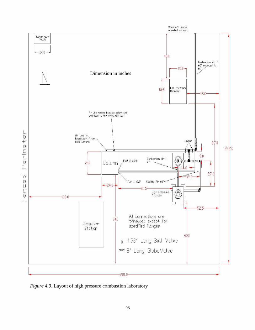
93
Figure 4.3. Layout of high pressure combustion laboratory
Dimension in inches

94
Figure 4.4. Layout of high pressure combustion laboratory
Dimension in inches

95
Figure 4.5. (a) Photographic image of combustion air pre-heater (b) Schematic diagram of
combustion air pre-heater
(a)
(b)
Flow
Dimensions in inches [mm]

96
Figure 4.6. Heater stand
Holes for securing heater to stand
Holes for securing stand to floor

97
Figure 4.7 Fuel station
Fuel tanks (10)
Portable fuel tanks
Compressor

98
Figure 4.8. Layout of fuel flow control system
Dimensions in inches
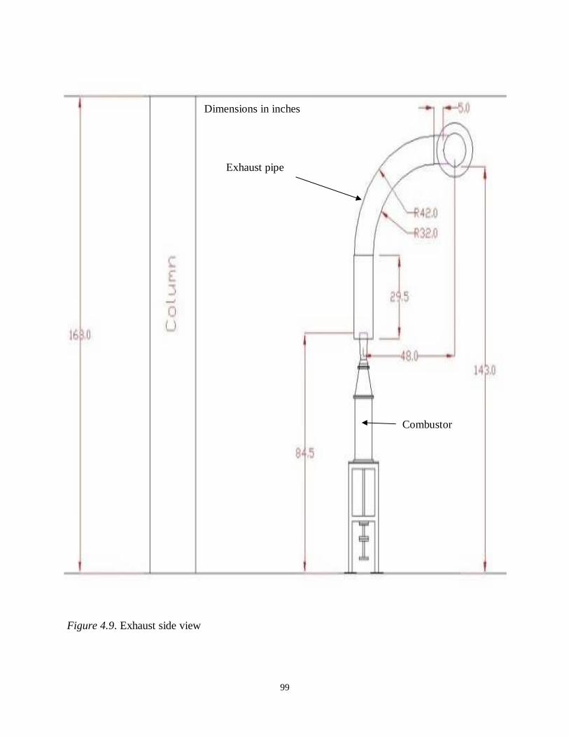
99
Figure 4.9. Exhaust side view
Dimensions in inches
Exhaust pipe
Combustor

100
Figure 4.10. Exhaust overhead view
Dimensions in inches
Low pressure combustor
High pressure combustor
Exhaust pipe
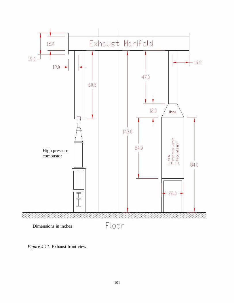
101
Figure 4.11. Exhaust front view
Dimensions in inches
High pressure combustor
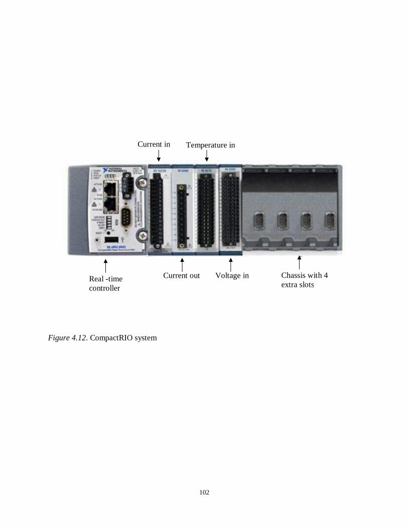
102
Figure 4.12. CompactRIO system
Real -time controller
Current in
Current out
Temperature in
Voltage in Chassis with 4 extra slots

103
Air/Fuel
Mix
Cooling
Air
Compressed
Air In
Electronic
Flow Control
Valve
Mass-flow
Controller
Manual
Control ValvesAbs. Pressure
Transducer
Diff. Pressure
Transducers
Type K
Thermocouples
Current
Out
Temp.
In
Current
In
Natural
Gas In
RS232Serial
Electric Heater
Digital Heater Control
Ethernet
To PC
CompactRIO DAQ System
Figure 4.13. Sensor/controller and CompactRIO Layout
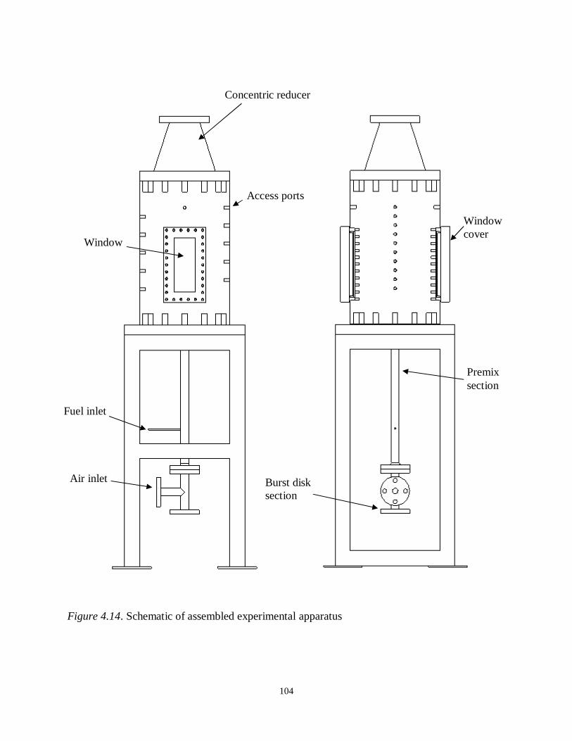
104
Figure 4.14. Schematic of assembled experimental apparatus
Concentric reducer
Window cover
Window
Access ports
Premix section
Fuel inlet
Air inlet Burst disk section

105
Figure 4.15. Exploded view of experimental apparatus
Window cover
Combustion chamber
Dump plane
Plenum base
Premix section
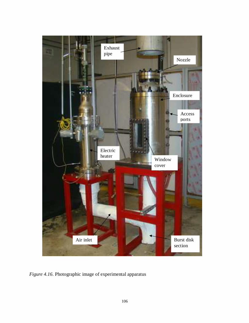
106
Figure 4.16. Photographic image of experimental apparatus
Enclosure
Window cover
Access ports
Exhaust pipe
Electric heater
Nozzle
Air inlet Burst disk section

107
Figure 4.17. Photographic image of experimental apparatus
Electric heater
Solenoid valve
Fuel line
Fuel inlet
Concentric reducer
Nozzle
Combustion chamber
Window
Dump plane

108
Figure 4.18. Photographic image of experimental apparatus
Fuel inlet
Cooling air hoses
Premix section
Window cover
Enclosure

109
Figure 4.19. Details of assembled plenum base
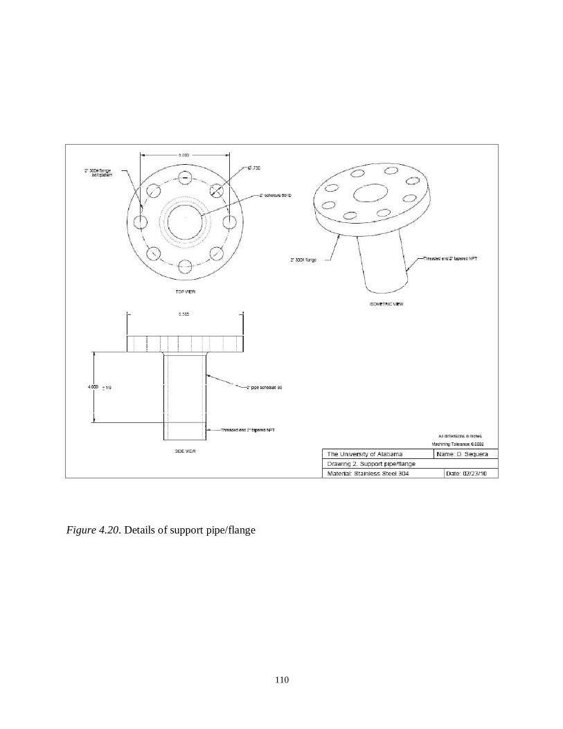
110
Figure 4.20. Details of support pipe/flange

111
Figure 4.21. Details of plenum base

112
Figure 4.22. Details of enclosure

113
Figure 4.23. Details of faces of enclosure
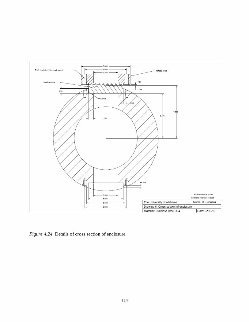
114
Figure 4.24. Details of cross section of enclosure

115
Figure 4.25. Details of windows on enclosure
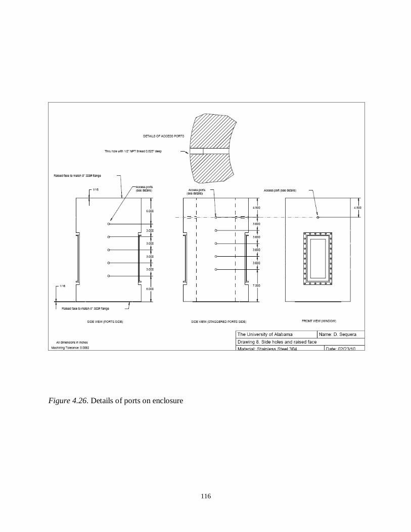
116
Figure 4.26. Details of ports on enclosure
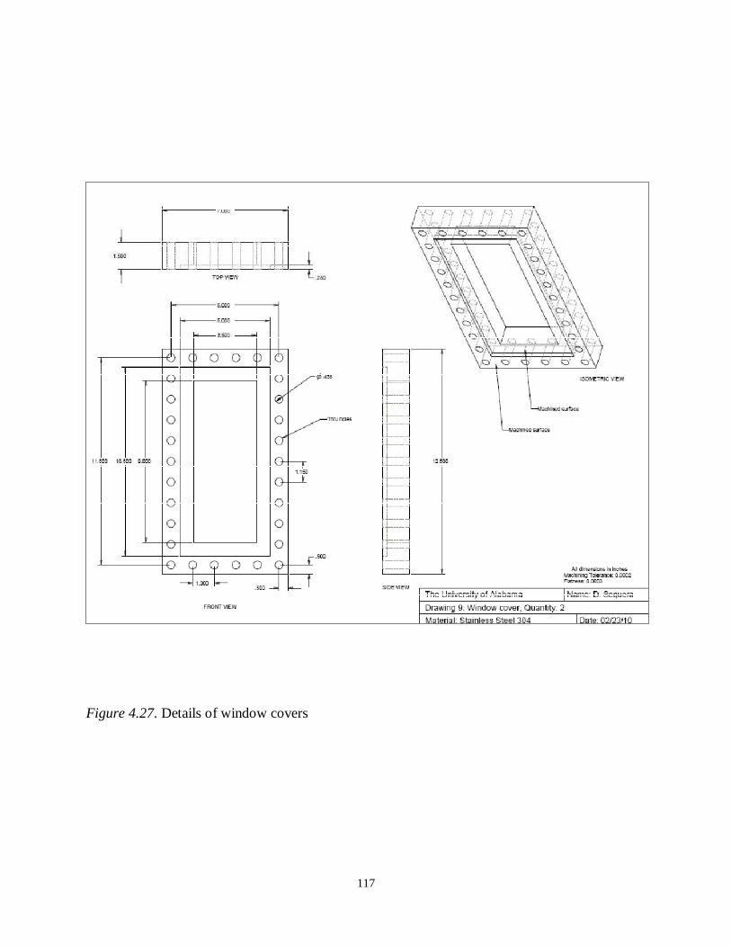
117
Figure 4.27. Details of window covers
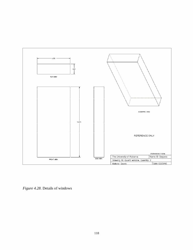
118
Figure 4.28. Details of windows

119
Figure 4.29 Schematic diagram and photograph of sampling probe
Stainless steel section Quartz section
Union
To gas analyzer
Fittings
To gas analyzer
Fitting (connects to wall of enclosure) Union
Gas sample

120
CHAPTER 5
REDUCTION OF COMBUSTION NOISE AND INSTABILITIES WITH THE USE OF POROUS INERT MATERIAL
Background
The stabilization mechanism of a swirl-stabilized combustor consists of inducing a
tangential or swirl velocity prior to reactants entering the combustion chamber. A sudden
expansion of the cross sectional area in the direction of the flow takes place as reactants enter the
combustion chamber. This sudden expansion of the swirling flow creates corner and central
recirculation zones, which in turn allow heat transfer from products to reactants, providing
ignition energy to incoming reactants. Corner recirculation zone is presumably the main source
of noise in swirl-stabilized flame, due to high turbulent fluctuations dominant in this region. A
numerical study presented in Chapter 2 revealed that use of porous insert in the corner
recirculation region redistributes the flow, mitigating highly turbulent structures that generate
noise.
Combustion instability is the result of the coupling of pressure waves generated by
unsteady heat release rate with those generated by oscillating pressure excitation of air
surrounding reaction zone. Typically active methods involving costly equipment that are difficult
to operate are used to control noise and instabilities. This investigation presents a passive
technique, requiring no control during operation, to reduce combustion noise. Furthermore,
combustion noise and combustion instabilities are different outcomes of the same fundamental

121
problem. Thus, reduction in combustion noise is a step forward to mitigate combustion
instabilities. The combustion process in gas turbines for power generation occurs at an elevated
pressure to improve thermal efficiency of the system. Previous experiments presented in Chapter
3 were conducted at atmospheric pressure, low reactant flow rates, and low air inlet
temperatures. Although these conditions are not typical of gas turbine combustors, the use of
PIM as a passive technique indicated significant reduction in combustion noise, and
consequently in combustion instabilities. In this chapter, experiments are conducted at conditions
replicating gas turbine combustor operation, with reactant inlet temperature of up to 260 °C, and
average reactant inlet velocity of up to 76 m/s, at fuel lean conditions with equivalence ratio
varying from 0.65 to 0.75. Corresponding, the reactant inlet Reynolds numbers vary from 2x10⁴
to 11x104(see Appendix E for details).
The present approach is similar to that presented in Chapter 3, i.e., a passive technique
that combines the features of a swirl stabilized flame with those of introducing a PIM in the
combustor to reduce combustion noise and instability. An experimental investigation simulating
conditions of a gas turbine engine, combining use of swirl flow and PIM to reduce combustion
noise and instabilities is lacking in the literature. Mechanical damage in gas turbine engines
caused by pressure fluctuations, driven by combustion instabilities, has been a recurring
problem. Down time and repairs associated with these problems are costly, and damages can be
catastrophic. This study finds relevance since the technique presented can significantly mitigate
combustion noise and instabilities at source. Specifically, PIM changes the velocity profiles and
turbulent structures inside the combustion chamber favorably, in such a way that turbulent
fluctuations are mitigated to eliminate dominant frequencies that produce noise and instabilities.

122
5.2 Experimental Setup
The experimental apparatus described in chapter 4 is shown schematically in Figure 5.1.
A compressor and dryer assembly supplied dry air at 200 psi. A ball valve and pressure regulator
were used to reduce pressure down to 60 psi. A control valve (Kammer model 0350E3-P) was
used to regulate the total air flow rate. Air supply was split into two lines: combustion air and
cooling air lines. Combustion air is mixed with fuel and participates in the combustion reaction.
Cooling air maintains the apparatus at a safe temperature and it does not participate in
combustion. Downstream of the split, globe valves on each air line were used to control the flow
rate in each line. Downstream of each valve, combustion and cooling air flows were measured
independently with identical LFE calibrated for 0 to 1400 lpm. Pressure drop across the LFE was
measured by a differential pressure transducer. An absolute pressure transducer was used to
measure the absolute pressure of air passing through the LFE. A k-type thermocouple was used
to measure the temperature of the air passing through the LFE. The flow rate measured by the
LFE is corrected for temperature and pressure as specified by the manufacturer (see Appendix C
for details).
Next, cooling air was routed directly to combustion apparatus. Flow of cooling air
surrounds the combustion chamber, inside an enclosure. Combustion air was routed through an
electrical heater (Osram Sylvania 72 KW model number 073377) used for preheating prior to the
air entering combustion apparatus. Downstream of the electric heater, pipes were insulated to
reduce heat loss. Combustion air then entered the premix section, where fuel is injected. The
premix section is a 60 cm (24 inches) long, 2.5 cm (1 inch) stainless steel schedule 80 pipe with
ID = 2.44 cm (0.96 inches) and OD = 3.35 cm (1.32 inches). Fuel and air mixed prior to entering
the combustion chamber.
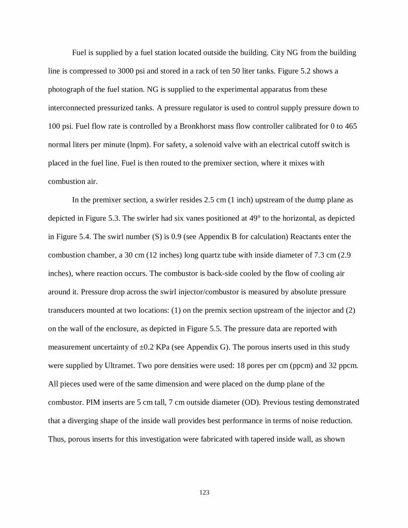
123
Fuel is supplied by a fuel station located outside the building. City NG from the building
line is compressed to 3000 psi and stored in a rack of ten 50 liter tanks. Figure 5.2 shows a
photograph of the fuel station. NG is supplied to the experimental apparatus from these
interconnected pressurized tanks. A pressure regulator is used to control supply pressure down to
100 psi. Fuel flow rate is controlled by a Bronkhorst mass flow controller calibrated for 0 to 465
normal liters per minute (lnpm). For safety, a solenoid valve with an electrical cutoff switch is
placed in the fuel line. Fuel is then routed to the premixer section, where it mixes with
combustion air.
In the premixer section, a swirler resides 2.5 cm (1 inch) upstream of the dump plane as
depicted in Figure 5.3. The swirler had six vanes positioned at 49° to the horizontal, as depicted
in Figure 5.4. The swirl number (S) is 0.9 (see Appendix B for calculation) Reactants enter the
combustion chamber, a 30 cm (12 inches) long quartz tube with inside diameter of 7.3 cm (2.9
inches), where reaction occurs. The combustor is back-side cooled by the flow of cooling air
around it. Pressure drop across the swirl injector/combustor is measured by absolute pressure
transducers mounted at two locations: (1) on the premix section upstream of the injector and (2)
on the wall of the enclosure, as depicted in Figure 5.5. The pressure data are reported with
measurement uncertainty of ±0.2 KPa (see Appendix G). The porous inserts used in this study
were supplied by Ultramet. Two pore densities were used: 18 pores per cm (ppcm) and 32 ppcm.
All pieces used were of the same dimension and were placed on the dump plane of the
combustor. PIM inserts are 5 cm tall, 7 cm outside diameter (OD). Previous testing demonstrated
that a diverging shape of the inside wall provides best performance in terms of noise reduction.
Thus, porous inserts for this investigation were fabricated with tapered inside wall, as shown

124
schematically in Figure 5.6. Porous insert was kept in place by press fitting the PIM into the
quartz chamber using a temperature resistant carbon foil, provided by Ultramet.
The product gas was sampled continuously by a quartz probe (OD = 5.0 mm) mounted on
the enclosure and traversed in the radial direction across the combustor. The probe was mounted
in two steps: (1) straight stainless steel section of the probe was connected to a fitting on wall of
enclosure on designated location (see Figure 5.5); (2) L-shape quartz section was connected to
straight stainless steel section using a union and fitting. The upstream tip of the probe was
tapered to 1 mm ID to quench reactions inside the probe. Figure 5.7 shows a diagram and
photograph of the sampling probe. The gas sample passed through an ice bath and water traps to
remove moisture prior to entering the gas analyzers. The dry sample was routed through
electrochemical analyzers to measure concentrations of CO and NOx in ppm. The analyzer also
measured oxygen and carbon dioxide concentrations used to cross-check the equivalence ratio
obtained from the measured fuel and air flow rates. The gas analyzer manufacturer reports a
measurement uncertainty of ±2 ppm on dry basis. Flame was ignited with the use of a high-
voltage spark generator. Poles of the generator were exposed to reactant flow and then generator
was activated to create a strong spark between the poles to ignite reactants. A low reactant flow
rate was used during ignition to avoid sudden pressure increase that could damage the sampling
probe.
For open top experiments, sound pressure data were measured outside the enclosure,
aligned with the exit plane at different locations. For restricted top experiments, sound pressure
data were measured at two different locations simultaneously, targeting two different sources of
noise: (1) within the enclosure, hereon referred to as combustion noise, (2) outside the enclosure,
hereon referred to as jet noise. Combustion noise data were acquired using a Kistler water-cooled

125
pressure sensor (model 601B1) with sensitivity of 1.132 pC/psi. A signal conditioner (model
Kistler 5051) converts the sensor output to voltage signal, digitized by the LabVIEW data
acquisition system. Pressure sensor is mounted on the wall of the enclosure, as illustrated in
Figure 5.5. Sensor probe for combustion noise measurements is exposed to pressure oscillations
resulting from coupling (or cancelling) of acoustic waves with waves driven by unsteady heat
release rate. Combustion noise sensor is also exposed to cooling air flow, thus to the turbulent
fluctuations associated with it. Jet noise is measured outside of the enclosure, thus, the probe is
exposed to pressure fluctuations induced by the high velocity jet at the nozzle exit. Jet noise
pressure data were collected using a Brüel & Kjær condenser microphone probe (Model 4189-A-
021) located at different positions outside the enclosure (sound pressure data for open top
experiments were acquired with the same instrument). The measured voltage signal is converted
to pressure fluctuation data using the calibrated probe sensitivity of 45.8 mV/Pa. Measurements
were acquired at sampling rates of 2000 and 4000 Hz. Signals from both instruments are
processed using FFT analysis to obtain the sound power spectra. A Matlab script (see Appendix
F for details) was written to compute the total sound pressure level (SPL) in decibels (dB), given
by (Bussman, 2001):
��� = 10 ∗ log�� ����������� �
Where Pref = 20 µPa. Total SPL was calculated by:
�������� = 10 ∗ log���∑ 10�.�∗����� �
(5.1)
(5.2)
126
Where SPLi is the SPL at each frequency band, and n is the number of frequency bands. One-
third octave frequency bands were used, from bands 13 to 29 for sampling rate of 2000 Hz and
from 13 to 32 for sampling rate of 4000 Hz.
5.3 Results and Discussion
Previously conducted experiments (Chapter 4) indicated a reduction of combustion noise
with the use of porous inserts in the reaction zone of a swirl stabilized flame. Reduction in noise
was achieved by re-distributing the flow of reactants and products within the combustion
chamber. Presence of porous material offers resistance to the incoming flow of reactants, thus, a
limited amount of flow penetrates the porous insert to eliminate the corner recirculation zone.
Combustion noise can be generated by the turbulent fluctuations dominant in the corner
recirculation zone. Thus, it follows that elimination of the corner recirculation zone would result
in reduced sound pressure levels. The flame is sustained and confined within the core region of
the porous insert. Products of this gas flame penetrate the porous insert through the inside wall
and mix with the reactants flowing through the PIM. The mixture of reactants and products exits
the porous insert, and ignites to sustain flamelets at the downstream surface of PIM, as illustrated
in Figure 5.8. Noise reduction can be expected to depend upon PIM pore density, and location
and geometry of the porous insert. PIM must target highly turbulent regions within the
combustor to be effective. Preliminary experiments indicated two types of free flame: (1)
anchored within the premixer tube downstream of the swirler, (2) stabilized within the quartz
combustor. Flame anchoring within the premixer tube was undesired because flame propagation
in turbulent recirculation zone downstream of swirler resulted in very high SPL. Increased
reactant flow rate resulted in flame stabilized within the combustor, which reduced the SPL.
127
Previous experiments (Chapter 3) were conducted at relatively low reactant inlet velocities (10
m/s). In this section, experiments were conducted at high reactant inlet velocities, closely
simulating inlet conditions of gas turbine engines. Experiments were conducted with combustion
air flow rates (Q) of 1020, 1400 and 2040 standard liters per minute (slpm), which yield bulk
inlet axial velocities of 30 to 76 m/s at atmospheric pressure (see Appendix E). Experiments
were conducted with no porous insert as the baseline case and then with tapered inserts of pore
density of 18 and 32 ppcm. Tests were conducted with open top (i.e., without the nozzle section
downstream of the combustion chamber) and with restricted top, whereby a nozzle section was
placed downstream of the enclosure.
Sound pressure measurements were taken to examine noise trends at different operating
conditions. First, with open top, five sets of data were taken to demonstrate repeatability of
measurements for Q = 1020 slpm, Ф = 0.7 and Tinlet = 20 °C and no supply of cooling air (Qc).
Microphone probe was aligned with the exit plane of the enclosure, as shown schematically in
Figure 5.9. Data were taken at distance (d) of 25 cm from axis of combustor. Figure 5.10 shows
that one third octave band SPL overlap one another, indicating measurements are repeatable.
Next, SPL was measured at 5 radial locations (d). The combustor was operated at Ф = 0.7 with
no supply of cooling air and no porous insert, Q = 1020 slpm and Tinlet = 20 °C. Table 5.1
provides a summary of the total SPL measured for each case. Figure 5.11 shows the measured
SPL spectra in one-third octave band. SPL spectra show similar trends for each case, while total
SPL decreases with increase in distance (d) of the measurement point. This result is expected due
to atmospheric attenuation of sound. Next, with restricted top, SPL was measured at 16 different
points surrounding the jet as shown schematically in Figure 5.12. Experiments were conducted
for Q = 1020 slpm, Ф = 0.7 with a porous insert of 18 ppcm and Tinlet = 20 °C. Cooling air flow
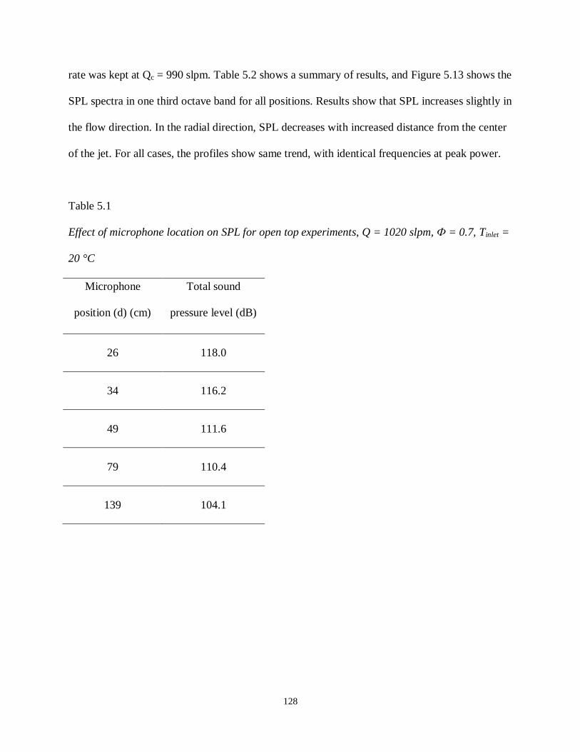
128
rate was kept at Qc = 990 slpm. Table 5.2 shows a summary of results, and Figure 5.13 shows the
SPL spectra in one third octave band for all positions. Results show that SPL increases slightly in
the flow direction. In the radial direction, SPL decreases with increased distance from the center
of the jet. For all cases, the profiles show same trend, with identical frequencies at peak power.
Table 5.1
Effect of microphone location on SPL for open top experiments, Q = 1020 slpm, Ф = 0.7, Tinlet =
20 °C
Microphone
position (d) (cm)
Total sound
pressure level (dB)
26 118.0
34 116.2
49 111.6
79 110.4
139 104.1

129
Table 5.2
Effect of microphone location on SPL for restricted top experiments, Q = 1020 slpm, Ф = 0.7,
Tinlet = 20 °C, Qc = 990 slpm
Microphone position #
(see Figure 5.12)
Total sound pressure
level (dB)
11 103.1
21 103.8
31 104.6
41 105.3
12 101.6
22 102.2
32 103.0
42 103.8
13 100.9
23 101.4
33 102.3
43 102.9
14 99.7
24 100.2
34 100.6
44 101.0
130
5.3.1 Open Top Experiments
(a) Effect of Pore Density
Experiments were conducted with open top enclosure for two combustion air flow rates
Q =1020 and 1400 slpm, pertaining to mass flow rates of 1.30 and 1.80 Kg/min, respectively.
Tests were conducted at three equivalence ratios (Ф): 0.65, 0.70 and 0.75 and three combustion
air inlet temperatures of Tinlet = 20, 130 and 260 °C. Experiments were conducted without porous
insert as the baseline case and with 18 ppcm and 32 ppcm porous inserts to investigate the effect
of pore size. Sound pressure measurements were taken at the exit plane of enclosure at d = 25
cm, as depicted in Figure 5.9. Figure 5.14 presents the power spectra without porous insert for Q
= 1020 slpm, Ф = 0.65, and different air inlet temperatures. Power spectra are presented in this
study to recognize dominant frequencies, if any. Thus, data are presented in linear scale, as
opposed to log scale involving dB. For Tinlet = 20 and 130 °C, power spectra appears broadband,
yet, at Tinlet = 130 °C, an instability is observed at 525 Hz. For Tinlet = 260 °C, there is dominant
frequency at 750 Hz signifying combustion instability, i.e., heat release oscillations are coupled
with acoustic oscillations. Observation during experiments also indicated instability: combustion
roar was noticeably louder with high pitch. Figure 5.15 shows the power spectra at Ф = 0.7 for
all air inlet temperatures. Results for Tinlet = 20 °C show broadband power spectra with a minor
peak centered around 400 Hz. However, for Tinlet = 130 °C the instability is dominant at 525 Hz.
At Tinlet = 260 °C, power spectra is broadband and no instability is present. Figure 5.16 shows
power spectra for Ф = 0.75. Instability is present for Tinlet = 130 °C only, but no distinct peak is
observed at other inlet air temperatures. These results show that changes in the equivalence ratio
and/or inlet air temperatures can manifest instabilities in the combustor.
131
Figure 5.17 shows power spectra for experiments conducted with porous insert of 18
ppcm, Q = 1020 slpm and all inlet air temperatures. Results show significant reduction in SPL
for all inlet air temperatures and, most importantly, instabilities present without porous insert
were completely mitigated. Flame under these conditions was confined within the inside walls of
the porous insert, with combustion also occurring on the downstream surface of the porous
insert. Thus, No combustion within the PIM (interior combustion) was present. Figures 5.18 and
5.19 show results with porous insert for Ф = 0.70 and 0.75 respectively. Results are similar to
those for Ф = 0.65, i.e., the dominant peak frequency indicative of combustion instability, was
eliminated by the use of porous insert. Total SPL was also reduced with use of PIM, and
reduction was particularly large for cases with instability in the baseline case as summarized in
Table 5.3. Results indicate SPL reduction of 4 to 9 dB. Figure 5.20 to 5.22 show power spectra
for cases studied with 32 ppcm porous insert. Again, porous insert eliminates combustion
instabilities and reduces total SPL, also summarized in Table 5.3. Use of 32 ppcm porous insert
also reduces SPL by up to 9 dB, principally for cases when combustion instability is present with
no porous insert. SPL obtained with 18 ppcm and 32 ppcm are comparable, thus, the effect of
pore size is not significant. Porous inserts of both pore densities are effective in reducing SPL.
Figure 5.23 shows SPL in dB versus one third octave bands for cases with Ф = 0.65 and Tinlet =
20, 130 and 260 °C. Porous insert mitigates fluctuations at higher frequencies: 400 Hz and
above. Both 18 and 32 ppcm porous inserts resulted in SPL reduction; however, difference
between them is not significant as discussed above. Figures 5.24 and 5.25 depict similar results
for Ф = 0.70 and 0.75, respectively. Clearly, porous insert reduces SPL by mitigating combustion
instabilities.
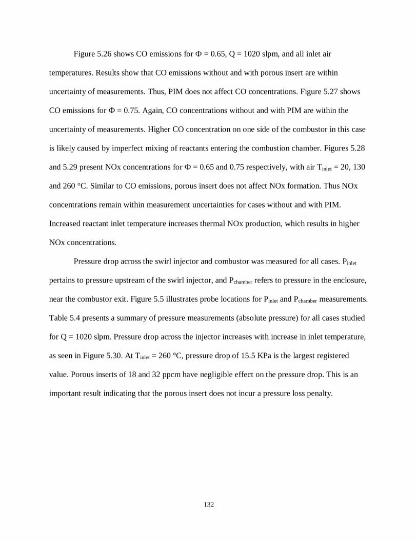
132
Figure 5.26 shows CO emissions for Ф = 0.65, Q = 1020 slpm, and all inlet air
temperatures. Results show that CO emissions without and with porous insert are within
uncertainty of measurements. Thus, PIM does not affect CO concentrations. Figure 5.27 shows
CO emissions for Ф = 0.75. Again, CO concentrations without and with PIM are within the
uncertainty of measurements. Higher CO concentration on one side of the combustor in this case
is likely caused by imperfect mixing of reactants entering the combustion chamber. Figures 5.28
and 5.29 present NOx concentrations for Ф = 0.65 and 0.75 respectively, with air Tinlet = 20, 130
and 260 °C. Similar to CO emissions, porous insert does not affect NOx formation. Thus NOx
concentrations remain within measurement uncertainties for cases without and with PIM.
Increased reactant inlet temperature increases thermal NOx production, which results in higher
NOx concentrations.
Pressure drop across the swirl injector and combustor was measured for all cases. Pinlet
pertains to pressure upstream of the swirl injector, and Pchamber refers to pressure in the enclosure,
near the combustor exit. Figure 5.5 illustrates probe locations for Pinlet and Pchamber measurements.
Table 5.4 presents a summary of pressure measurements (absolute pressure) for all cases studied
for Q = 1020 slpm. Pressure drop across the injector increases with increase in inlet temperature,
as seen in Figure 5.30. At Tinlet = 260 °C, pressure drop of 15.5 KPa is the largest registered
value. Porous inserts of 18 and 32 ppcm have negligible effect on the pressure drop. This is an
important result indicating that the porous insert does not incur a pressure loss penalty.

133
Table 5.3
Summary of sound pressure levels for Q=1020 slpm
Tinlet (°C) Ф Qc (slpm)
Total sound pressure level (dB)
No PIM 18 ppcm PIM 32 ppcm PIM
20
0.65 990 117.0 110.2 111.4
0.70 990 120.0 111.7 111.0
0.75 990 120.6 114.9 113.2
130
0.65 1160 120.5 113.9 114.7
0.70 1160 125.8 116.4 116.4
0.75 1160 124.3 118.3 116.2
260
0.65 1350 122.1 117.4 118.2
0.70 1350 119.0 119.0 118.2
0.75 1350 118.8 119.8 118.8
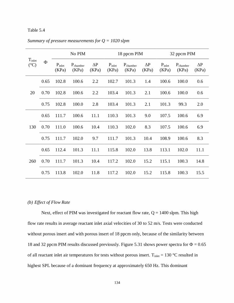
134
Table 5.4
Summary of pressure measurements for Q = 1020 slpm
Tinlet (°C)
Ф
No PIM 18 ppcm PIM 32 ppcm PIM
Pinlet (KPa)
Pchamber (KPa)
∆P (KPa)
Pinlet (KPa)
Pchamber (KPa)
∆P (KPa)
Pinlet (KPa)
Pchamber (KPa)
∆P (KPa)
20
0.65 102.8 100.6 2.2 102.7 101.3 1.4 100.6 100.0 0.6
0.70 102.8 100.6 2.2 103.4 101.3 2.1 100.6 100.0 0.6
0.75 102.8 100.0 2.8 103.4 101.3 2.1 101.3 99.3 2.0
130
0.65 111.7 100.6 11.1 110.3 101.3 9.0 107.5 100.6 6.9
0.70 111.0 100.6 10.4 110.3 102.0 8.3 107.5 100.6 6.9
0.75 111.7 102.0 9.7 111.7 101.3 10.4 108.9 100.6 8.3
260
0.65 112.4 101.3 11.1 115.8 102.0 13.8 113.1 102.0 11.1
0.70 111.7 101.3 10.4 117.2 102.0 15.2 115.1 100.3 14.8
0.75 113.8 102.0 11.8 117.2 102.0 15.2 115.8 100.3 15.5
(b) Effect of Flow Rate
Next, effect of PIM was investigated for reactant flow rate, Q = 1400 slpm. This high
flow rate results in average reactant inlet axial velocities of 30 to 52 m/s. Tests were conducted
without porous insert and with porous insert of 18 ppcm only, because of the similarity between
18 and 32 ppcm PIM results discussed previously. Figure 5.31 shows power spectra for Ф = 0.65
of all reactant inlet air temperatures for tests without porous insert. Tinlet = 130 °C resulted in
highest SPL because of a dominant frequency at approximately 650 Hz. This dominant

135
frequency was also present for cases with Ф = 0.70 and 0.75, as seen in Figures 5.32 and 5.33
respectively. For cases with Tinlet = 20 and 260 °C, power spectra was broadband with no distinct
peaks. Thus, the total SPL for Tinlet = 130 °C was highest for all Ф. Similar to cases with lower
reactant flow rates, porous inserts resulted in significant reduction of SPL and combustion
instability. Figure 5.34 shows power spectra with 18 ppcm PIM. Results show that for all Tinlet,
power spectra were broadband. Most importantly, dominant frequency present at Tinlet = 130 °C
indicative of combustion instability was completely mitigated. Similarly, Figure 5.35 shows that
dominant frequency of combustion instability at Ф = 0.7 was mitigated by porous insert. Figure
5.36 (c) shows a peak at 400 Hz with the porous insert. In this case, localized interior combustion
was present at the downstream surface of the porous insert. This finding is consistent with
previous results in Chapter 3 indicating that PIM interior combustion is not desirable. Despite an
increase in reactant velocity by 40%, PIM remains effective in reducing SPL and mitigating
combustion instability.
Length of the porous insert is an important geometric parameter. Preliminary
experiments, not shown here, demonstrated that PIM with shorter length (2.5 cm) had small
effect in reducing SPL. With a longer porous insert, a larger percentage of products of the
confined free flame penetrate the PIM through the inner wall. Thus, heat is transferred and
distributed more effectively by PIM. Table 5.5 presents a summary of total SPL obtained for all
cases with Q = 1400 slpm. Results indicate that, similar to Q = 1020 slpm, PIM reduces the total
SPL and mitigates combustion instability. However, case with PIM and Tinlet = 260 ° C resulted
in higher SPL than that without PIM because of localized interior combustion. Figures 5.37 to
5.39 compare SPL without and with PIM. Results indicate a favorable trend with the use of PIM,
particularly at frequencies higher than 400 Hz. Figures 5.40 to 5.43 show CO and NOx emissions
136
for Q = 1400 slpm. Similar to Q = 1020 slpm, CO emissions were not affected by the PIM.
Further, CO emissions were nearly independent of the reactant inlet temperature. NOx emissions
presented in Figure 5.43 show an increase with inlet air temperature as expected. However, NOx
formation was not affected by the PIM.
Table 5.6 presents a summary of pressure drop data measured across the swirl injector
and combustor for Q = 1400 slpm. Similar to cases with Q = 1020 slpm, pressure drop increased
with inlet air temperature and it was highest for Tinlet = 260 °C, as seen in Figure 5.44. Flow
resistance by the porous insert is minor compared to the overall pressure drop in the swirler and
combustor.
Table 5.5
Summary of sound pressure levels for Q=1400 slpm
Tinlet (°C) Ф Qc (slpm) Total sound pressure level (dB)
No PIM PIM (18 ppcm)
20
0.65 1300 118.0 113.6
0.70 1300 120.4 115.6
0.75 1300 120.8 116.6
130
0.65 1550 124.3 117.8
0.70 1550 125.6 119.0
0.75 1550 125.4 120.5
260
0.65 1750 119.6 119.7
0.70 1750 119.1 121.3
0.75 1750 119.2 122.8

137
Table 5.6
Summary of pressure measurements for Q = 1400 slpm
Tinlet (°C)
Ф No PIM 18 ppcm PIM
Pinlet (KPa)
Pchamber (KPa)
∆P (KPa)
Pinlet (KPa)
Pchamber (KPa)
∆P (KPa)
20
0.65 105.5 102.0 3.5 105.5 101.3 4.2
0.70 106.1 101.3 4.8 105.5 100.6 4.9
0.75 105.5 102.0 3.5 105.5 100.6 4.9
130
0.65 113.0 102.0 11.0 111.7 101.3 10.4
0.70 113.7 101.3 12.4 113.1 101.3 11.8
0.75 113.0 102.0 11.0 112.4 102.0 10.4
260
0.65 118.6 102.0 16.6 117.2 101.3 15.9
0.70 118.6 101.3 17.3 119.3 102.0 17.3
0.75 117.9 102.0 15.9 119.3 102.0 17.3
5.3.2 Restricted Top Experiments
(a) Effect of PIM on Noise at P = 1 atm
Experiments were conducted with the reducer and exit nozzle installed to independently
investigate effect of porous insert on combustion noise and jet noise. Tests were conducted with
a 7.6 cm by 3.8 cm tapered exit nozzle. Figure 5.45 shows a schematic diagram of the nozzle
used for these experiments. This size nozzle did not build pressure inside the enclosure during
testing, thus tests pertain nearly to atmospheric pressure. Sound pressure data were measured
138
simultaneously at two locations: (1) outside the enclosure to obtain SPL of the high velocity jet,
or jet noise; and (2) on the wall of the enclosure, to obtain SPL in the reaction zone, or
combustion noise. First, sound pressure data were collected at two different sampling rates to
identify possible frequency aliasing. Figure 5.46 shows the power spectra of jet noise at 2000
and 4000 Hz sampling rates for the baseline case of Ф = 0.70 and Tinlet = 130 °C. Figures 5.46 (a)
and (b) both show a frequency peak at 600 Hz, indicating lack of frequency aliasing by sampling
rate. Figure 5.47 shows the power spectra for combustion noise data at 2000 and 4000 Hz
collected by the pressure sensor. Figure 5.47 (a) shows a peak frequency at 725 Hz, and 5.47 (b)
shows a peak at 1250 Hz, suggesting signal aliasing. Thus, subsequent measurements for both jet
noise and combustion noise were taken at 4000 Hz. Sound pressure data at jet exit were collected
at three different locations along the axis of the jet, as depicted in Figure 5.48. Figure 5.49
presents SPL versus one-third octave bands for Ф = 0.70 and Tinlet = 20, 130 and 260 °C. For
Tinlet = 20 °C, SPL is broadband for all microphone locations. Case with Tinlet = 130 °C shows a
dominant peak at 600 Hz. Case with Tinlet = 260 °C shows peaks at 800 Hz and 1600 Hz. In
general, microphone at location 3, farthest from the nozzle exit, registers highest total SPL for all
cases. Nonetheless, power spectra shows similar trends at each probe location. Thus, subsequent
results are presented only for data collected at location 1, i.e., for probe aligned with the jet exit
plane.
Figures 5.50 and 5.51 present power spectra at jet exit without porous insert and with 18
ppcm insert, respectively, for Ф = 0.65 and Tinlet = 20, 130 and 260 °C. As observed with
experiments in the previous section, PIM insert resulted in reduction of noise and mitigation of
combustion instability (notice change in vertical scale). Use of porous insert affects sound
pressure in the reaction zone, which in turn affects noise generated at the nozzle exit. This is the
139
result of the acoustic attenuation of pressure waves generated at the reaction zone by the
presence of PIM. Figure 5.52 compares SPL without and with porous insert for Ф = 0.65. Results
show that PIM is effective in reducing SPL, particularly at frequencies higher than 500 Hz.
Figures 5.53 and 5.54 present the combustion noise power spectra without and with PIM
respectively. As observed before, instability present without PIM, observed in Figure 5.53 (c) at
1250 Hz, was mitigated with use of PIM. Power spectra shown in Figure 5.54 have low power
for all cases. Next, Figure 5.55 presents combustion noise without and with porous insert for Ф =
0.65 and Tinlet = 20, 130 and 260 °C. Similar to jet noise results, use of PIM reduces combustion
noise and mitigates combustion instabilities in the reaction zone.
Next, jet noise and combustion noise data are presented for Ф = 0.70, without and with
porous insert in Figures 5.56 and 5.57, respectively. Figure 5.56 (b) shows a dominant peak at
550 Hz without porous insert, which is mitigated with use of PIM, as shown in Figure 5.57 (b).
Figure 5.58 compares SPL without and with PIM for Ф = 0.70. Case without PIM results in high
SPL at high frequencies. These high peaks are suppressed with the use of PIM. Next, similar to
jet noise, combustion noise power spectra are presented in Figures 5.59 and 5.60. For these
cases, noise is mainly broadband, except a peak present at 1250 Hz for Tinlet = 130 °C for no PIM
case. As observed before, this peak is eliminated by use of PIM. Figure 5.61 compares SPL for
Ф = 0.7 without and with PIM. As before, PIM reduces SPL by eliminating combustion
instability and attenuating broadband noise. Figures 5.62 to 5.67 present results for Ф = 0.75 for
jet noise and combustion noise. Again, results are consistent with previous observations at lower
equivalence ratios. A summary of test results is presented in Table 5.7 for jet noise, and Table
5.8 for combustion noise.
140
Similar to previous experiments, pressure drop across swirler and combustor was also
measured. Table 5.9 presents a summary of pressure drop data without and with porous insert.
Increase in inlet air temperature increases the pressure drop, which is highest at 12.4 KPa for
Tinlet = 260 °C, as seen in Figure 5.68. As observed for previous cases, PIM has negligible effect
on pressure drop across the injector/combustor.
Porous insert in the combustor reduces SPL and eliminates dominant frequencies of
fluctuation, caused by combustion instability. This result was consistently observed for all cases
operated at atmospheric pressure. Results show that porous insert reduces total SPL by
approximately 1-2 dB for cases with broadband noise. Most importantly, combustion instability
is also mitigated by PIM with SPL reduction of nearly 10 dB. In summary, when combustion
instability is present, PIM eliminates it or mitigates it, and when the combustion instability is not
present, PIM reduces broadband combustion noise.

141
Table 5.7
Summary of jet noise total SPL, Q = 1020 slpm, P = 1 atm
Total sound pressure level (dB)
Tinlet (°C) Ф Qc (slpm) Position No PIM 18 ppcm PIM
20
0.65 990
1 104.5 102.8
2 106.0 104.4
3 106.7 105.1
0.70 990
1 106.6 104.1
2 108.3 105.5
3 109.0 106.0
0.75 990
1 108.2 105.9
2 109.8 107.7
3 110.4 108.5
130
0.65 1160
1 111.6 105.1
2 113.3 106.6
3 113.5 107.5
0.70 1160
1 118.7 106.7
2 121.0 108.7
3 122.7 109.1
0.75 1160
1 125.0 109.1
2 125.2 111.2
3 124.1 112.3
260
0.65 1350
1 116.6 108.2
2 117.0 110.1
3 117.2 111.1
0.70 1350
1 112.6 110.4
2 115.1 112.3
3 115.4 113.3
0.75 1350
1 114.4 111.6
2 117.4 113.6
3 117.5 114.3
142
Table 5.8
Summary of combustion noise total SPL, Q = 1020 slpm, P = 1 atm
Total sound pressure level (dB)
Tinlet (°C) Ф Qc (slpm) No PIM 18 ppcm PIM
20
0.65 990 145.6 145.0
0.70 990 145.7 144.8
0.75 990 146.0 144.9
130
0.65 1160 146.7 145.0
0.70 1160 148.0 145.1
0.75 1160 157.5 145.5
260
0.65 1350 149.3 145.4
0.70 1350 147.4 145.9
0.75 1350 147.6 146.3

143
Table 5.9
Summary of pressure measurements for restricted top experiments, Q = 1020 slpm, P = 1 atm
Tinlet (°C)
Ф No PIM 18 ppcm PIM
Pinlet (KPa)
Pchamber (KPa)
∆P (KPa)
Pinlet (KPa)
Pchamber (KPa)
∆P (KPa)
20
0.65 104.1 102.7 1.4 104.8 103.4 1.4
0.70 104.8 103.4 1.4 104.8 104.1 0.7
0.75 104.1 103.4 0.7 104.8 104.1 0.7
130
0.65 109.6 104.8 4.8 114.4 104.8 9.6
0.70 111.0 103.4 7.6 113.1 105.5 7.6
0.75 111.7 104.1 7.6 113.7 105.5 8.2
260
0.65 116.5 104.8 11.7 116.5 106.2 10.3
0.70 117.2 105.5 11.7 117.9 106.8 11.1
0.75 118.6 106.2 12.4 117.2 106.2 11.0
(b) Effect of PIM on Noise at Elevated Pressure
In this section, experiments were conducted with a tapered nozzle of 3.8 cm by 1.9 cm,
illustrated in Figure 5.69. Previous experiments conducted with cold flow through this nozzle
resulted in high pressure inside the enclosure. Tests were conducted with Q = 2040 slpm, Ф =
0.65, 0.70 and 0.75 and enclosure pressure of approximately 2 atm. Figures 5.70 to 5.72 show
the SPL in one third octave bands for combustion noise. Cases without porous insert have
dominant frequencies above 500 Hz. Similar to previous results, PIM effectively reduces these
high frequency fluctuations. Table 5.10 shows a summary of obtained results for elevated
pressure tests. Results indicate that PIM is also beneficial at elevated pressures, however, total
SPL reduction is limited to 1-2 dB, thus, decrease in total SPL is not as dramatic. Based on
144
previous observations, flame is presumably partly submerged within the PIM, however, direct
flame observation was not feasible in the present setup. Table 5.11 shows a summary of pressure
measurements, which are also illustrated in Figure 5.73. Highest pressure drop of 9.0 KPa,
pertains to Tinlet = 130 °C. At Tinlet = 260 °C, pressure sensor exceeded operating temperature and
failed to generate signal.
Table 5.10
Summary of combustion noise total SPL, Q = 2040 slpm, P = 2 atm
Total sound pressure level (dB)
Tinlet (°C) Ф Qc (slpm) No PIM 18 ppcm PIM
20
0.65 1230 148.9 146.6
0.70 1230 148.8 148.1
0.75 1230 149.4 152.5
130
0.65 1700 148.8 147.7
0.70 1700 148.5 147.0
0.75 1700 148.2 146.2
260
0.65 1900 148.3 146.8
0.70 1900 149.8 146.7
0.75 1900 150.3 146.6

145
Table 5.11
Summary of pressure measurements for restricted top experiments, Q = 2040 slpm, P = 2 atm
Tinlet (°C)
Ф No PIM 18 ppcm PIM
Pinlet (KPa)
Pchamber (KPa)
∆P (KPa) Pinlet
(KPa) Pchamber (KPa)
∆P (KPa)
20
0.65 236.5 234.4 2.1 209.6 208.2 1.4
0.70 238.6 237.2 1.4 212.4 210.3 2.1
0.75 243.4 241.3 2.1 212.4 210.5 1.9
130
0.65 249.6 243.4 6.2 228.9 221.3 7.6
0.70 252.4 245.5 6.9 233.1 224.1 9.0
0.75 258.6 250.3 8.3 234.4 225.5 8.9
260
0.65 249.6 - - 242.0 233.7 8.3
0.70 254.4 - - 243.4 235.1 8.3
0.75 257.2 - - 246.8 - -
5.4 Conclusions
Experiments were conducted at high inlet air flow rates, and high air inlet temperature to
more closely simulate operating conditions of a gas turbine engine. Average axial velocity at
combustor inlet for conditions ranged from 30 to 76 m/s. Inlet air temperatures were 20, 130 and
260 °C and equivalence ratios were 0.65, 0.70 and 0.75. Effect of pore density was investigated,
using 18 and 32 ppcm porous inserts. Jet noise and combustion noise were measured
independently. Tests were conducted at chamber pressure P = 1 and 2 atm. Pressure drop across
swirl injector and combustor was also measured. Product gas was sampled to measure CO and
NOx concentrations. Results demonstrated that porous insert reduce total SPL for all cases.

146
Furthermore, combustion instability present without porous insert was mitigated by use of PIM
in the reaction zone. Porous media redistributes incoming flow and attenuates turbulent flow
fluctuations, eliminates corner recirculation zone, and effectively attenuates sound pressure
levels. Porous media attenuates heat release fluctuations associated with turbulent nature of
flame. This result was obtained only with combustion occurring on the surface of the porous
insert. PIM interior combustion tends to increase SPL, and thus, it is undesirable. For flow
conditions investigated, flame stabilized within core region and on surface of PIM for both pore
densities. Difference between PIM of 18 and 32 ppcm is not significant. Highest pressure drop
registered pertained highest inlet temperature. PIM did not affect CO or NOx emissions for cases
studied.
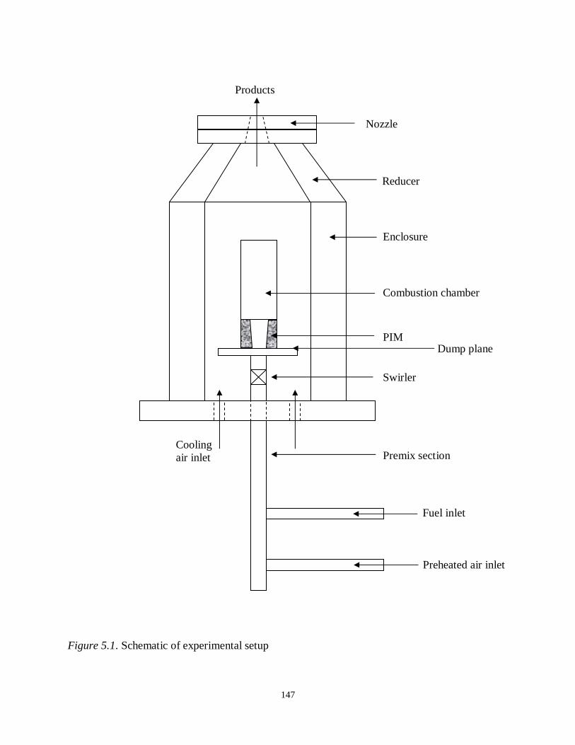
147
Figure 5.1. Schematic of experimental setup
Cooling air inlet
Reducer
Nozzle
Enclosure
Combustion chamber
PIM
Swirler
Premix section
Fuel inlet
Preheated air inlet
Products
Dump plane

148
Figure 5.2. Photograph of fuel station
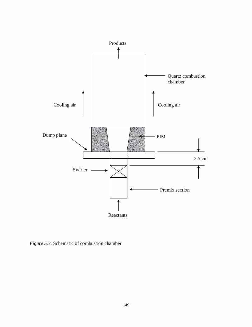
149
Figure 5.3. Schematic of combustion chamber
Quartz combustion chamber
PIM
Swirler
Premix section
2.5 cm
Reactants
Cooling air Cooling air
Products
Dump plane

150
Figure 5.4. Swirler
Flow
Flow
1.18
48.9°
R.02
R.26 R.30
0.50 .25 0.40
0.04
0.04
0.21 Ø0.96
Ø0.54

151
Figure 5.5. Schematic of experimental setup
Cooling air inlet
Reducer
Nozzle
Enclosure
Swirler
Fuel inlet
Preheated air inlet
Products
Port for Pinlet measurement
Port for Tinlet measurement
Port for Pchamber measurement
Port for emissions measurement
27 cm

152
Figure 5.6. Schematic diagram of PIM
5
3.75
2.5
7
Direction of the flow
Dimensions in cm

153
Figure 5.7. Schematic diagram and photograph of sampling probe
Stainless steel section Quartz section
Union
To gas analyzer
Fittings
To gas analyzer
Fitting (connects to wall of enclosure) Union
Gas sample

154
Figure 5.8. Schematic of PIM stabilization mechanism
Surface flame
Reactants
Products
PIM
Swirler
Reactants
Core region flame

155
Figure 5.9. Microphone locations for open top experiments
d=80
d=25
d=35
d=50
d=140
Dimensions in cm
Cooling air inlet
Enclosure
Fuel inlet
Preheated air inlet

156
Figure 5.10. One third octave band SPL for repeatability test
Frequency (Hz)
SP
L(d
B)
0 200 400 600 800 100060
70
80
90
100
110
120
130

157
Figure 5.11. Effect of probe position on SPL for open top experiments, Q = 1020 slpm, Ф = 0.7,
Tinlet = 20 °C
Frequency (Hz)
SP
L(d
B)
0 200 400 600 800 100050
60
70
80
90
100
110
120
130
d = 25 cmd = 35 cmd = 50 cmd = 80 cmd = 140 cm

158
Figure 5.12. Microphone locations for restricted top experiments
11
2.5
2.5
2.5
21
31
12
2.5
41
2.5 2.5
22
32
42
13
23
33
43
14
24
34
44
Dimensions in cm
25
Cooling air inlet
Reducer
Nozzle
Enclosure
Fuel inlet
Preheated air inlet

159
Figure 5.13. Effect of microphone location on SPL for restricted top experiments, Q = 1020
slpm, Ф = 0.7, Tinlet = 20 °C, Qc = 990 slpm
X
XXXX
XXX
XX
XX
X
X X
X
X
Frequency (Hz)
SP
L(d
B)
0 200 400 600 800 100065
70
75
80
85
90
95
100
105
Position 11Position 21Position 31Position 41
XX
XXX
X
XXXXX
X
X
X
X X
X
X
Frequency (Hz)S
PL
(dB
)0 200 400 600 800 100065
70
75
80
85
90
95
100
105
Position 12Position 22Position 32Position 42
X
XXXXX
XXXX
X X
X
XX X
X
X
Frequency (Hz)
SP
L(d
B)
0 200 400 600 800 100065
70
75
80
85
90
95
100
105
Position 13Position 23Position 33Position 43
XXXXXX
XXXX
X X
X
X
X X
X
X
Frequency (Hz)
SP
L(d
B)
0 200 400 600 800 100065
70
75
80
85
90
95
100
105
Position 14Position 24Position 34Position 44
X

160
Figure 5.14. Power spectra for Q = 1020 slpm, Ф = 0.65, no PIM (a) Tinlet = 20 °C, (b) Tinlet =
130 °C, (c) Tinlet = 260 °C
(a)
(b)
(c)
Frequency (Hz)
Po
we
r(A
.U.)
0 200 400 600 800 10000
5
10
15
Frequency (Hz)
Po
wer
(A.U
.)
0 200 400 600 800 10000
5
10
15
Frequency (Hz)
Po
we
r(A
.U.)
0 200 400 600 800 10000
5
10
15

161
Figure 5.15. Power spectra for Q = 1020 slpm, Ф = 0.70, no PIM (a) Tinlet = 20 °C, (b) Tinlet =
130 °C, (c) Tinlet = 260°C
(b)
(c)
(a)
Frequency (Hz)
Po
we
r(A
.U.)
0 200 400 600 800 10000
5
10
15
Frequency (Hz)
Po
we
r(A
.U.)
0 200 400 600 800 10000
5
10
15
Frequency (Hz)
Po
we
r(A
.U.)
0 200 400 600 800 10000
5
10
15
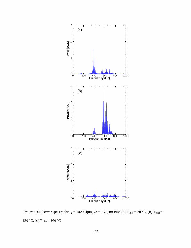
162
Figure 5.16. Power spectra for Q = 1020 slpm, Ф = 0.75, no PIM (a) Tinlet = 20 °C, (b) Tinlet =
130 °C, (c) Tinlet = 260 °C
(b)
(c)
(a)
Frequency (Hz)
Po
we
r(A
.U.)
0 200 400 600 800 10000
5
10
15
Frequency (Hz)
Po
wer
(A.U
.)
0 200 400 600 800 10000
5
10
15
Frequency (Hz)
Po
we
r(A
.U.)
0 200 400 600 800 10000
5
10
15

163
Figure 5.17. Power spectra for Q = 1020 slpm, Ф = 0.65, 18ppcm PIM (a) Tinlet = 20 °C, (b) Tinlet
= 130 °C, (c) Tinlet = 260 °C
(b)
(c)
(a)
Frequency (Hz)
Po
we
r(A
.U.)
0 200 400 600 800 10000
5
10
15
Frequency (Hz)
Po
we
r(A
.U.)
0 200 400 600 800 10000
5
10
15
Frequency (Hz)
Po
we
r(A
.U.)
0 200 400 600 800 10000
5
10
15

164
Figure 5.18. Power spectra for Q = 1020 slpm, Ф = 0.70, 18 ppcm PIM (a) Tinlet = 20 °C, (b)
Tinlet = 130 °C, (c) Tinlet = 260 °C
(b)
(c)
(a)
Frequency (Hz)
Po
we
r(A
.U.)
0 200 400 600 800 10000
5
10
15
Frequency (Hz)
Po
we
r(A
.U.)
0 200 400 600 800 10000
5
10
15
Frequency (Hz)
Po
we
r(A
.U.)
0 200 400 600 800 10000
5
10
15
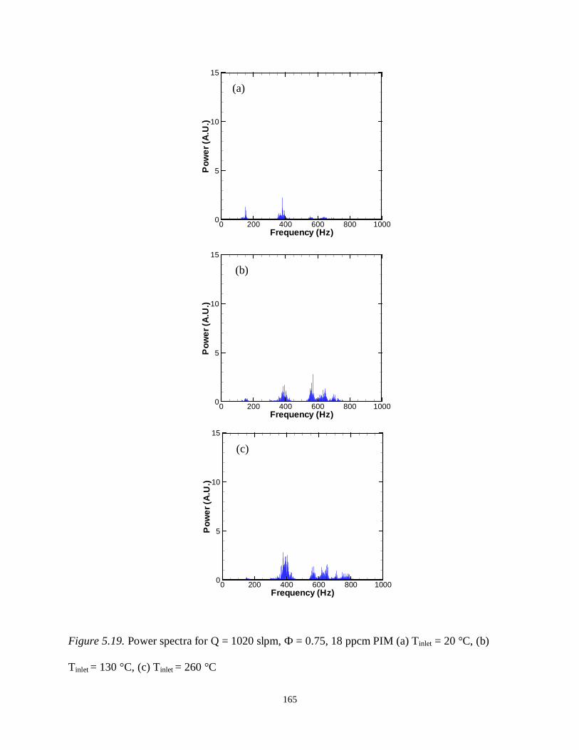
165
Figure 5.19. Power spectra for Q = 1020 slpm, Ф = 0.75, 18 ppcm PIM (a) Tinlet = 20 °C, (b)
Tinlet = 130 °C, (c) Tinlet = 260 °C
(b)
(c)
(a)
Frequency (Hz)
Po
we
r(A
.U.)
0 200 400 600 800 10000
5
10
15
Frequency (Hz)
Po
we
r(A
.U.)
0 200 400 600 800 10000
5
10
15
Frequency (Hz)
Po
we
r(A
.U.)
0 200 400 600 800 10000
5
10
15

166
Figure 5.20. Power spectra for Q = 1020 slpm, Ф = 0.65, 32 ppcm PIM (a) Tinlet = 20 °C, (b)
Tinlet = 130 °C, (c) Tinlet = 260 °C
(b)
(c)
(a)
Frequency (Hz)
Po
wer
(A.U
.)0 200 400 600 800 1000
0
5
10
15
Frequency (Hz)
Po
we
r(A
.U.)
0 200 400 600 800 10000
5
10
15
Frequency (Hz)
Po
wer
(A.U
.)
0 200 400 600 800 10000
5
10
15

167
Figure 5.21. Power spectra for Q = 1020 slpm, Ф = 0.70, 32 ppcm PIM (a) Tinlet = 20 °C, (b)
Tinlet = 130 °C, (c) Tinlet = 260 °C
(b)
(c)
(a)
Frequency (Hz)
Po
wer
(A.U
.)0 200 400 600 800 1000
0
5
10
15
Frequency (Hz)
Po
wer
(A.U
.)
0 200 400 600 800 10000
5
10
15
Frequency (Hz)
Po
wer
(A.U
.)
0 200 400 600 800 10000
5
10
15
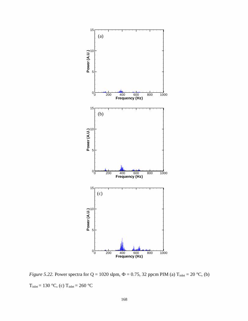
168
Figure 5.22. Power spectra for Q = 1020 slpm, Ф = 0.75, 32 ppcm PIM (a) Tinlet = 20 °C, (b)
Tinlet = 130 °C, (c) Tinlet = 260 °C
(b)
(c)
(a)
Frequency (Hz)
Po
wer
(A.U
.)
0 200 400 600 800 10000
5
10
15
Frequency (Hz)
Po
we
r(A
.U.)
0 200 400 600 800 10000
5
10
15
Frequency (Hz)
Po
we
r(A
.U.)
0 200 400 600 800 10000
5
10
15
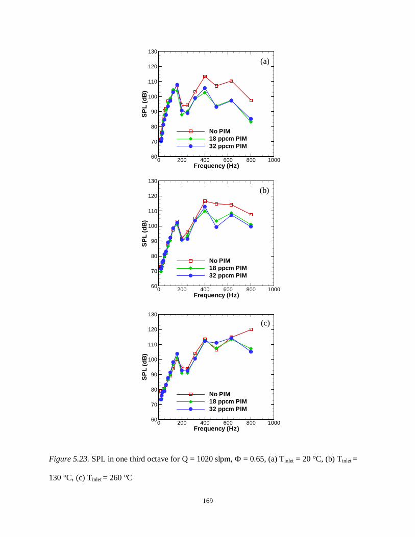
169
Figure 5.23. SPL in one third octave for Q = 1020 slpm, Ф = 0.65, (a) Tinlet = 20 °C, (b) Tinlet =
130 °C, (c) Tinlet = 260 °C
Frequency (Hz)
SP
L(d
B)
0 200 400 600 800 100060
70
80
90
100
110
120
130
No PIM18 ppcm PIM32 ppcm PIM
Frequency (Hz)
SP
L(d
B)
0 200 400 600 800 100060
70
80
90
100
110
120
130
No PIM18 ppcm PIM32 ppcm PIM
Frequency (Hz)
SP
L(d
B)
0 200 400 600 800 100060
70
80
90
100
110
120
130
No PIM18 ppcm PIM32 ppcm PIM
(b)
(c)
(a)
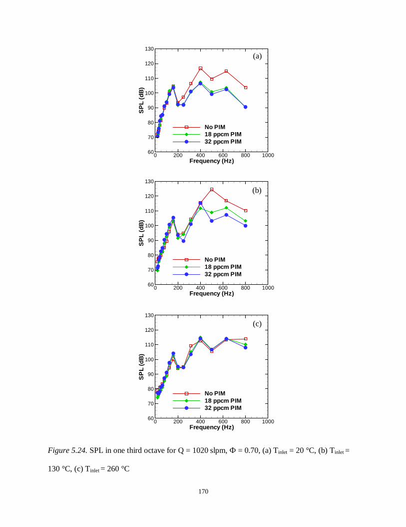
170
Figure 5.24. SPL in one third octave for Q = 1020 slpm, Ф = 0.70, (a) Tinlet = 20 °C, (b) Tinlet =
130 °C, (c) Tinlet = 260 °C
Frequency (Hz)
SP
L(d
B)
0 200 400 600 800 100060
70
80
90
100
110
120
130
No PIM18 ppcm PIM32 ppcm PIM
Frequency (Hz)
SP
L(d
B)
0 200 400 600 800 100060
70
80
90
100
110
120
130
No PIM18 ppcm PIM32 ppcm PIM
Frequency (Hz)
SP
L(d
B)
0 200 400 600 800 100060
70
80
90
100
110
120
130
No PIM18 ppcm PIM32 ppcm PIM
(b)
(c)
(a)

171
Figure 5.25. SPL in one third octave for Q = 1020 slpm, Ф = 0.75, (a) Tinlet = 20 °C, (b) Tinlet =
130 °C, (c) Tinlet = 260 °C
(b)
(c)
(a)
Frequency (Hz)
SP
L(d
B)
0 200 400 600 800 100060
70
80
90
100
110
120
130
No PIM18 ppcm PIM32 ppcm PIM
Frequency (Hz)
SP
L(d
B)
0 200 400 600 800 100060
70
80
90
100
110
120
130
No PIM18 ppcm PIM32 ppcm PIM
Frequency (Hz)
SP
L(d
B)
0 200 400 600 800 100060
70
80
90
100
110
120
130
No PIM18 ppcm PIM32 ppcm PIM
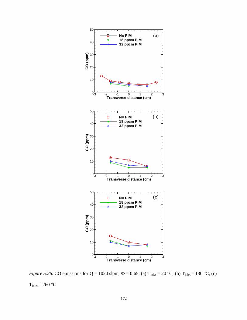
172
Figure 5.26. CO emissions for Q = 1020 slpm, Ф = 0.65, (a) Tinlet = 20 °C, (b) Tinlet = 130 °C, (c)
Tinlet = 260 °C
Transverse distance (cm)
CO
(pp
m)
-3 -2 -1 0 1 2 30
10
20
30
40
50
No PIM18 ppcm PIM32 ppcm PIM
Transverse distance (cm)
CO
(pp
m)
-3 -2 -1 0 1 2 30
10
20
30
40
50
No PIM18 ppcm PIM32 ppcm PIM
Transverse distance (cm)
CO
(pp
m)
-3 -2 -1 0 1 2 30
10
20
30
40
50
No PIM18 ppcm PIM32 ppcm PIM
(b)
(c)
(a)
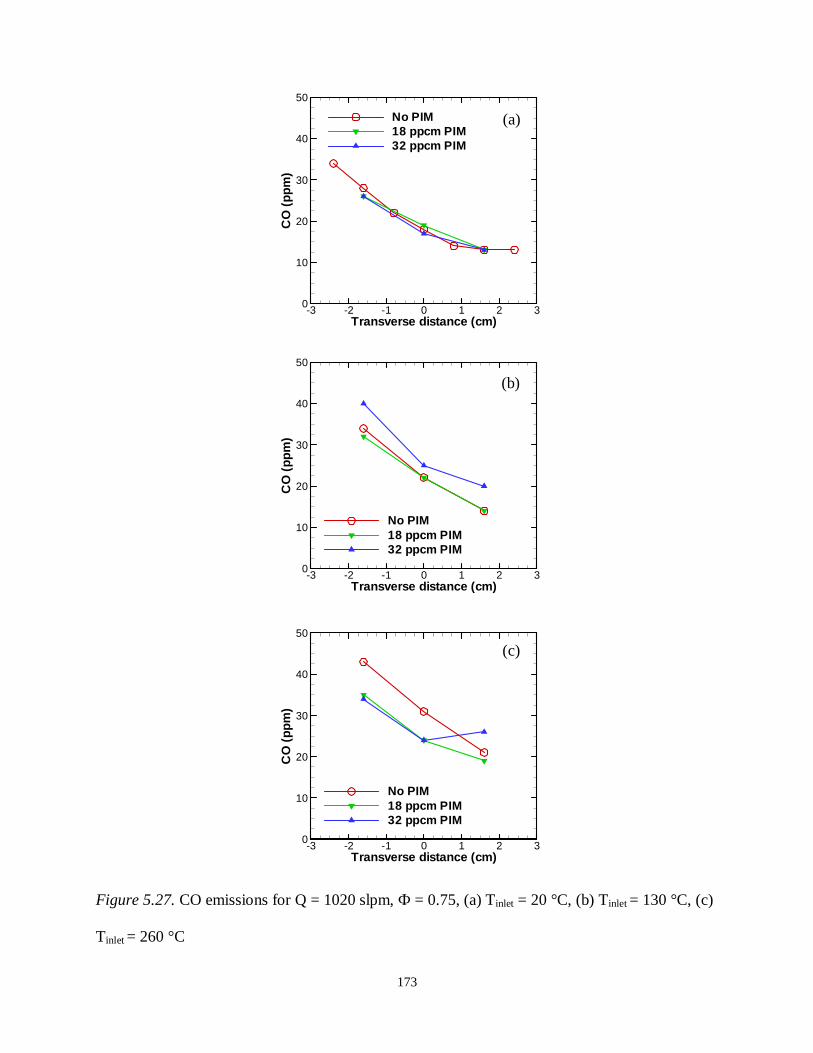
173
Figure 5.27. CO emissions for Q = 1020 slpm, Ф = 0.75, (a) Tinlet = 20 °C, (b) Tinlet = 130 °C, (c)
Tinlet = 260 °C
Transverse distance (cm)
CO
(pp
m)
-3 -2 -1 0 1 2 30
10
20
30
40
50
No PIM18 ppcm PIM32 ppcm PIM
Transverse distance (cm)
CO
(pp
m)
-3 -2 -1 0 1 2 30
10
20
30
40
50
No PIM18 ppcm PIM32 ppcm PIM
Transverse distance (cm)
CO
(pp
m)
-3 -2 -1 0 1 2 30
10
20
30
40
50
No PIM18 ppcm PIM32 ppcm PIM
(b)
(c)
(a)
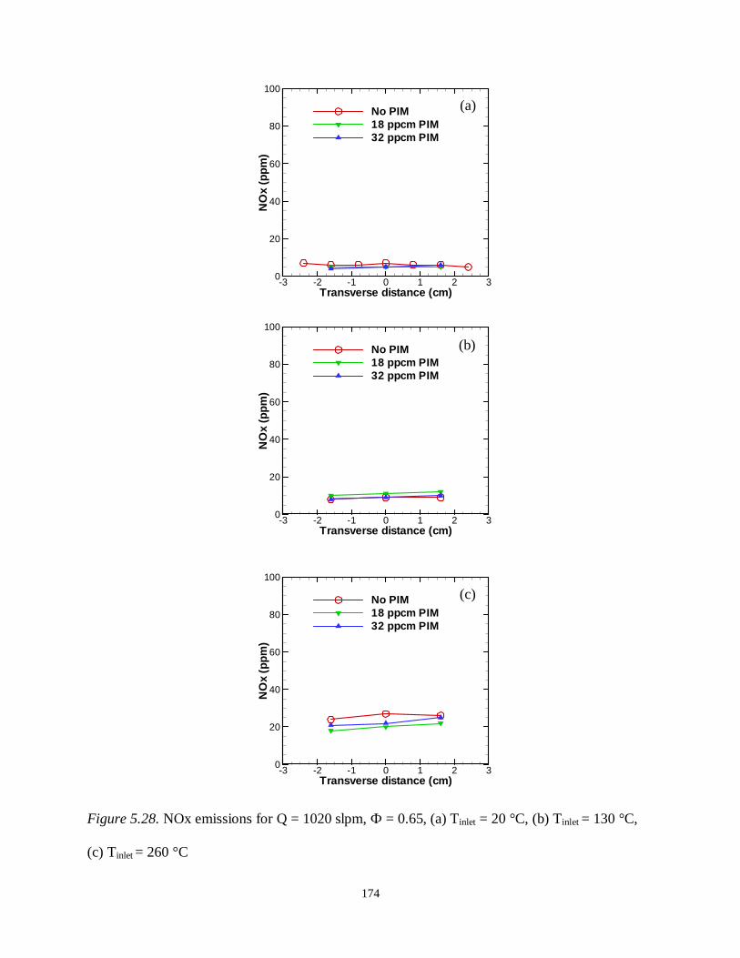
174
Figure 5.28. NOx emissions for Q = 1020 slpm, Ф = 0.65, (a) Tinlet = 20 °C, (b) Tinlet = 130 °C,
(c) Tinlet = 260 °C
Transverse distance (cm)
NO
x(p
pm
)
-3 -2 -1 0 1 2 30
20
40
60
80
100
No PIM18 ppcm PIM32 ppcm PIM
Transverse distance (cm)
NO
x(p
pm
)
-3 -2 -1 0 1 2 30
20
40
60
80
100
No PIM18 ppcm PIM32 ppcm PIM
Transverse distance (cm)
NO
x(p
pm
)
-3 -2 -1 0 1 2 30
20
40
60
80
100
No PIM18 ppcm PIM32 ppcm PIM
(b)
(c)
(a)

175
Figure 5.29. NOx emissions for Q = 1020 slpm, Ф = 0.75, (a) Tinlet = 20 °C, (b) Tinlet = 130 °C,
(c) Tinlet = 260 °C
Transverse distance (cm)
NO
x(p
pm
)-3 -2 -1 0 1 2 3
0
20
40
60
80
100
No PIM18 ppcm PIM32 ppcm PIM
Transverse distance (cm)
NO
x(p
pm
)
-3 -2 -1 0 1 2 30
20
40
60
80
100
No PIM18 ppcm PIM32 ppcm PIM
Transverse distance (cm)
NO
x(p
pm
)
-3 -2 -1 0 1 2 30
20
40
60
80
100
No PIM18 ppcm PIM32 ppcm PIM
(b)
(c)
(a)

176
Figure 5.30. Pressure drop measurements for open top experiments Q = 1020 slpm (a) no PIM
(b) 18 ppcm PIM (c) 32 ppcm PIM
(b)
(c)
(a)
Φ
∆P
(KP
a)
0.65 0.7 0.750
5
10
15
20
25
Tinlet = 20 oCTinlet = 130 oCTinlet = 260 oC
Φ
∆P
(KP
a)
0.65 0.7 0.750
5
10
15
20
25
Tinlet = 20 oCTinlet = 130 oCTinlet = 260 oC
Φ
∆P
(KP
a)
0.65 0.7 0.750
5
10
15
20
25
Tinlet = 20 oCTinlet = 130 oCTinlet = 260 oC

177
Figure 5.31. Power spectra for Q = 1400 slpm, Ф = 0.65, no PIM, (a) Tinlet = 20 °C, (b) Tinlet =
130 °C, (c) Tinlet = 260 °C
(b)
(c)
(a)
Frequency (Hz)
Po
we
r(A
.U.)
0 200 400 600 800 10000
5
10
15
Frequency (Hz)
Po
we
r(A
.U.)
0 200 400 600 800 10000
5
10
15
Frequency (Hz)
Po
we
r(A
.U.)
0 200 400 600 800 10000
5
10
15

178
Figure 5.32. Power spectra for Q = 1400 slpm, Ф = 0.70, no PIM, (a) Tinlet = 20 °C, (b) Tinlet =
130 °C, (c) Tinlet = 260°C
(b)
(c)
(a)
Frequency (Hz)
Po
we
r(A
.U.)
0 200 400 600 800 10000
5
10
15
Frequency (Hz)
Po
we
r(A
.U.)
0 200 400 600 800 10000
5
10
15
Frequency (Hz)
Po
we
r(A
.U.)
0 200 400 600 800 10000
5
10
15

179
Figure 5.33. Power spectra for Q = 1400 slpm, Ф = 0.75, no PIM, (a) Tinlet = 20 °C, (b) Tinlet =
130 °C, (c) Tinlet = 260 °C
(b)
(c)
(a)
Frequency (Hz)
Po
wer
(A.U
.)
0 200 400 600 800 10000
5
10
15
Frequency (Hz)
Po
wer
(A.U
.)
0 200 400 600 800 10000
5
10
15
Frequency (Hz)
Po
we
r(A
.U.)
0 200 400 600 800 10000
5
10
15

180
Figure 5.34. Power spectra for Q = 1400 slpm, Ф = 0.65, 18 ppcm PIM, (a) Tinlet = 20 °C, (b)
Tinlet = 130 °C, (c) Tinlet = 260 °C
(b)
(c)
(a)
Frequency (Hz)
Po
wer
(A.U
.)
0 200 400 600 800 10000
5
10
15
Frequency (Hz)
Po
wer
(A.U
.)
0 200 400 600 800 10000
5
10
15
Frequency (Hz)
Po
we
r(A
.U.)
0 200 400 600 800 10000
5
10
15

181
Figure 5.35. Power spectra for Q = 1400 slpm, Ф = 0.70, 18 ppcm PIM, (a) Tinlet = 20 °C, (b)
Tinlet = 130 °C, (c) Tinlet = 260°C
(b)
(c)
(a)
Frequency (Hz)
Po
wer
(A.U
.)
0 200 400 600 800 10000
5
10
15
Frequency (Hz)
Po
wer
(A.U
.)
0 200 400 600 800 10000
5
10
15
Frequency (Hz)
Po
we
r(A
.U.)
0 200 400 600 800 10000
5
10
15
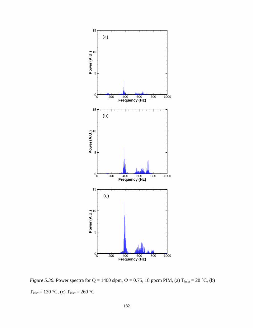
182
Figure 5.36. Power spectra for Q = 1400 slpm, Ф = 0.75, 18 ppcm PIM, (a) Tinlet = 20 °C, (b)
Tinlet = 130 °C, (c) Tinlet = 260 °C
(b)
(c)
(a)
Frequency (Hz)
Po
wer
(A.U
.)
0 200 400 600 800 10000
5
10
15
Frequency (Hz)
Po
we
r(A
.U.)
0 200 400 600 800 10000
5
10
15
Frequency (Hz)
Po
we
r(A
.U.)
0 200 400 600 800 10000
5
10
15

183
Figure 5.37. SPL in one third octave for Q = 1400 slpm, Ф = 0.65, (a) Tinlet = 20 °C, (b) Tinlet =
130 °C, (c) Tinlet = 260 °C
(b)
(c)
(a)
Frequency (Hz)
SP
L(d
B)
0 200 400 600 800 100060
70
80
90
100
110
120
130
No PIM18 ppcm PIM
Frequency (Hz)
SP
L(d
B)
0 200 400 600 800 100060
70
80
90
100
110
120
130
No PIM18 ppcm PIM
Frequency (Hz)
SP
L(d
B)
0 200 400 600 800 100060
70
80
90
100
110
120
130
No PIM18 ppcm PIM

184
Figure 5.38. SPL in one third octave for Q = 1400 slpm, Ф = 0.70, (a) Tinlet = 20 °C, (b) Tinlet =
130 °C, (c) Tinlet = 260 °C
(b)
(c)
(a)
Frequency (Hz)
SP
L(d
B)
0 200 400 600 800 100060
70
80
90
100
110
120
130
No PIM18 ppcm PIM
Frequency (Hz)
SP
L(d
B)
0 200 400 600 800 100060
70
80
90
100
110
120
130
No PIM18 ppcm PIM
Frequency (Hz)
SP
L(d
B)
0 200 400 600 800 100060
70
80
90
100
110
120
130
No PIM18 ppcm PIM

185
Figure 5.39. SPL in one third octave for Q = 1400 slpm, Ф = 0.75, (a) Tinlet = 20 °C, (b) Tinlet =
130 °C, (c) Tinlet = 260 °C
(b)
(c)
(a)
Frequency (Hz)
SP
L(d
B)
0 200 400 600 800 100060
70
80
90
100
110
120
130
No PIM18 ppcm PIM
Frequency (Hz)
SP
L(d
B)
0 200 400 600 800 100060
70
80
90
100
110
120
130
No PIM18 ppcm PIM
Frequency (Hz)
SP
L(d
B)
0 200 400 600 800 100060
70
80
90
100
110
120
130
No PIM18 ppcm PIM

186
Figure 5.40. CO emissions for Q = 1400 slpm, Ф = 0.65, (a) Tinlet = 20 °C, (b) Tinlet = 130 °C, (c)
Tinlet = 250 °C
Transverse distance (cm)
CO
(pp
m)
-3 -2 -1 0 1 2 30
10
20
30
40
50
60
70
No PIM18 ppcm PIM
Transverse distance (cm)
CO
(pp
m)
-3 -2 -1 0 1 2 30
10
20
30
40
50
60
70
No PIM18 ppcm PIM
Transverse distance (cm)
CO
(pp
m)
-3 -2 -1 0 1 2 30
10
20
30
40
50
60
70
No PIM18 ppcm PIM
(b)
(c)
(a)

187
Figure 5.41. CO emissions for Q = 1400 slpm, Ф = 0.75, (a) Tinlet = 20 °C, (b) Tinlet = 130 °C, (c)
Tinlet = 250 °C
Transverse distance (cm)
CO
(pp
m)
-3 -2 -1 0 1 2 30
10
20
30
40
50
60
70
No PIM18 ppcm PIM
Transverse distance (cm)
CO
(pp
m)
-3 -2 -1 0 1 2 30
10
20
30
40
50
60
70
No PIM18 ppcm PIM
Transverse distance (cm)
CO
(pp
m)
-3 -2 -1 0 1 2 30
10
20
30
40
50
60
70
No PIM18 ppcm PIM
(b)
(c)
(a)

188
Figure 5.42. NOx emissions for Q = 1400 slpm, Ф = 0.65, (a) Tinlet = 20 °C, (b) Tinlet = 130 °C,
(c) Tinlet = 260 °C
(b)
(c)
(a)
Transverse distance (cm)
NO
x(p
pm
)
-3 -2 -1 0 1 2 30
20
40
60
80
100
No PIM18 ppcm PIM
Transverse distance (cm)
NO
x(p
pm
)
-3 -2 -1 0 1 2 30
20
40
60
80
100
No PIM18 ppcm PIM
Transverse distance (cm)
NO
x(p
pm
)
-3 -2 -1 0 1 2 30
20
40
60
80
100
No PIM18 ppcm PIM

189
Figure 5.43. NOx emissions for Q = 1400 slpm, Ф = 0.75, (a) Tinlet = 20 °C, (b) Tinlet = 130 °C,
(c) Tinlet = 260 °C
(b)
(c)
(a)
Transverse distance (cm)
NO
x(p
pm
)
-3 -2 -1 0 1 2 30
20
40
60
80
100
120
No PIM18 ppcm PIM
Transverse distance (cm)
NO
x(p
pm
)
-3 -2 -1 0 1 2 30
20
40
60
80
100
120
No PIM18 ppcm PIM
Transverse distance (cm)
NO
x(p
pm
)
-3 -2 -1 0 1 2 30
20
40
60
80
100
120
No PIM18 ppcm PIM

190
Figure 5.44. Pressure drop measurements for open top experiments Q = 1400 slpm (a) no PIM
(b) 18 ppcm PIM
(b)
(a)
Φ
∆P
(KP
a)
0.65 0.7 0.750
5
10
15
20
25
Tinlet = 20 oCTinlet = 130 oCTinlet = 260 oC
Φ
∆P
(KP
a)
0.65 0.7 0.750
5
10
15
20
25
Tinlet = 20 oCTinlet = 130 oCTinlet = 260 oC
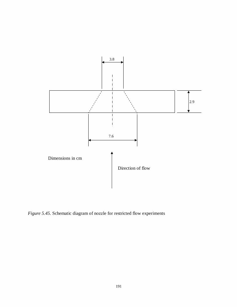
191
Figure 5.45. Schematic diagram of nozzle for restricted flow experiments
Dimensions in cm
Direction of flow
7.6
3.8
2.9

192
Figure 5.46. Jet noise power spectra, no PIM, P = 1 atm, Ф = 0.75, Tinlet = 130 °C (a) sampling
rate of 2000 Hz, (b) sampling rate of 4000 Hz
(b)
(a)
Frequency (Hz)
Po
wer
(A.U
.)
0 500 1000 1500 20000
20
40
60
80
100
120
Frequency (Hz)
Po
wer
(A.U
.)
0 500 1000 1500 20000
20
40
60
80
100
120
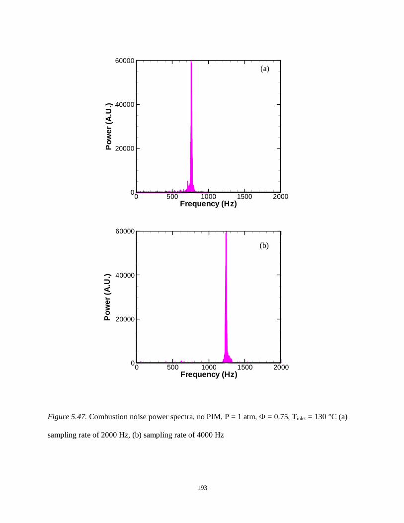
193
Figure 5.47. Combustion noise power spectra, no PIM, P = 1 atm, Ф = 0.75, Tinlet = 130 °C (a)
sampling rate of 2000 Hz, (b) sampling rate of 4000 Hz
(b)
(a)
Frequency (Hz)
Po
wer
(A.U
.)
0 500 1000 1500 20000
20000
40000
60000
Frequency (Hz)
Pow
er(A
.U.)
0 500 1000 1500 20000
20000
40000
60000
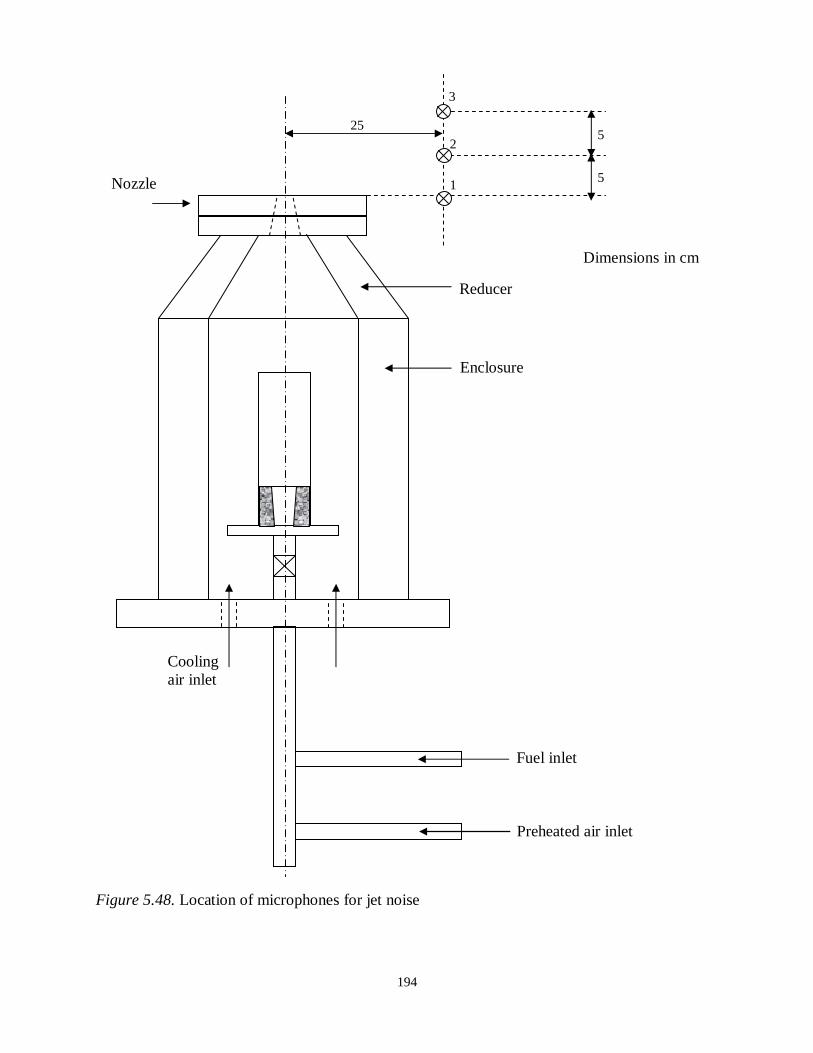
194
Figure 5.48. Location of microphones for jet noise
Dimensions in cm
25
Cooling air inlet
Reducer
Nozzle
Enclosure
Fuel inlet
Preheated air inlet
5
5 2
1
3
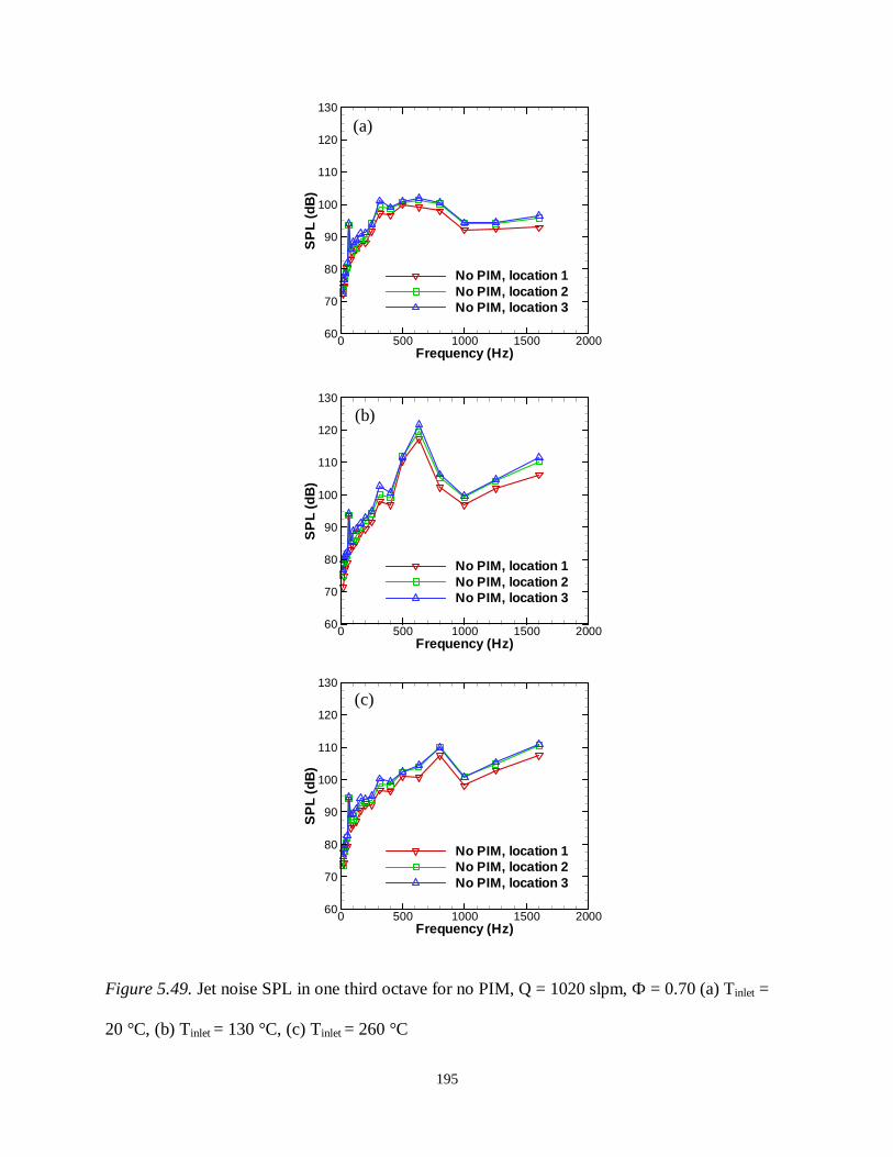
195
Figure 5.49. Jet noise SPL in one third octave for no PIM, Q = 1020 slpm, Ф = 0.70 (a) Tinlet =
20 °C, (b) Tinlet = 130 °C, (c) Tinlet = 260 °C
(b)
(c)
(a)
Frequency (Hz)
SP
L(d
B)
0 500 1000 1500 200060
70
80
90
100
110
120
130
No PIM, location 1No PIM, location 2No PIM, location 3
Frequency (Hz)
SP
L(d
B)
0 500 1000 1500 200060
70
80
90
100
110
120
130
No PIM, location 1No PIM, location 2No PIM, location 3
Frequency (Hz)
SP
L(d
B)
0 500 1000 1500 200060
70
80
90
100
110
120
130
No PIM, location 1No PIM, location 2No PIM, location 3
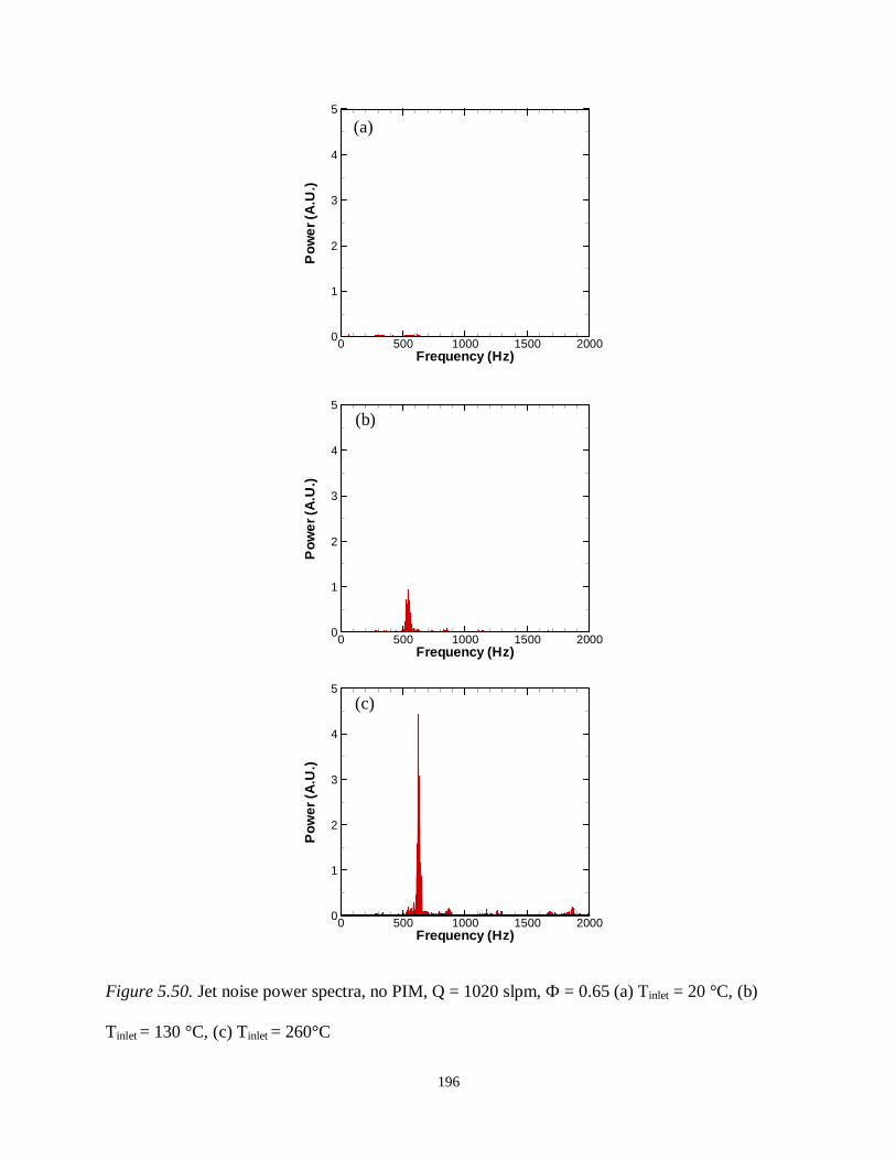
196
Figure 5.50. Jet noise power spectra, no PIM, Q = 1020 slpm, Ф = 0.65 (a) Tinlet = 20 °C, (b)
Tinlet = 130 °C, (c) Tinlet = 260°C
(b)
(c)
(a)
Frequency (Hz)
Po
we
r(A
.U.)
0 500 1000 1500 20000
1
2
3
4
5
Frequency (Hz)
Po
we
r(A
.U.)
0 500 1000 1500 20000
1
2
3
4
5
Frequency (Hz)
Po
wer
(A.U
.)
0 500 1000 1500 20000
1
2
3
4
5
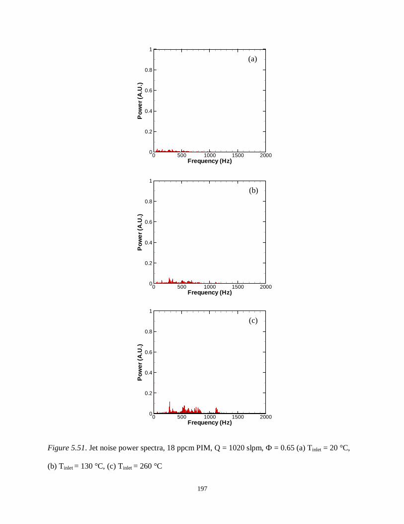
197
Figure 5.51. Jet noise power spectra, 18 ppcm PIM, Q = 1020 slpm, Ф = 0.65 (a) Tinlet = 20 °C,
(b) Tinlet = 130 °C, (c) Tinlet = 260 °C
Frequency (Hz)
Po
we
r(A
.U.)
0 500 1000 1500 20000
0.2
0.4
0.6
0.8
1
Frequency (Hz)
Po
wer
(A.U
.)
0 500 1000 1500 20000
0.2
0.4
0.6
0.8
1
(b)
(c)
(a)
Frequency (Hz)
Po
we
r(A
.U.)
0 500 1000 1500 20000
0.2
0.4
0.6
0.8
1

198
Figure 5.52. Jet noise SPL in one third octave, Q = 1020 slpm, Ф = 0.65, P = 1 atm, (a) Tinlet =
20 °C, (b) Tinlet = 130 °C, (c) Tinlet = 260 °C
(b)
(c)
(a)
Frequency (Hz)
SP
L(d
B)
0 500 1000 1500 200060
70
80
90
100
110
120
130
No PIM18 ppcm PIM
Frequency (Hz)
SP
L(d
B)
0 500 1000 1500 200060
70
80
90
100
110
120
130
No PIM18 ppcm PIM
Frequency (Hz)
SP
L(d
B)
0 500 1000 1500 200060
70
80
90
100
110
120
130
No PIM18 ppcm PIM
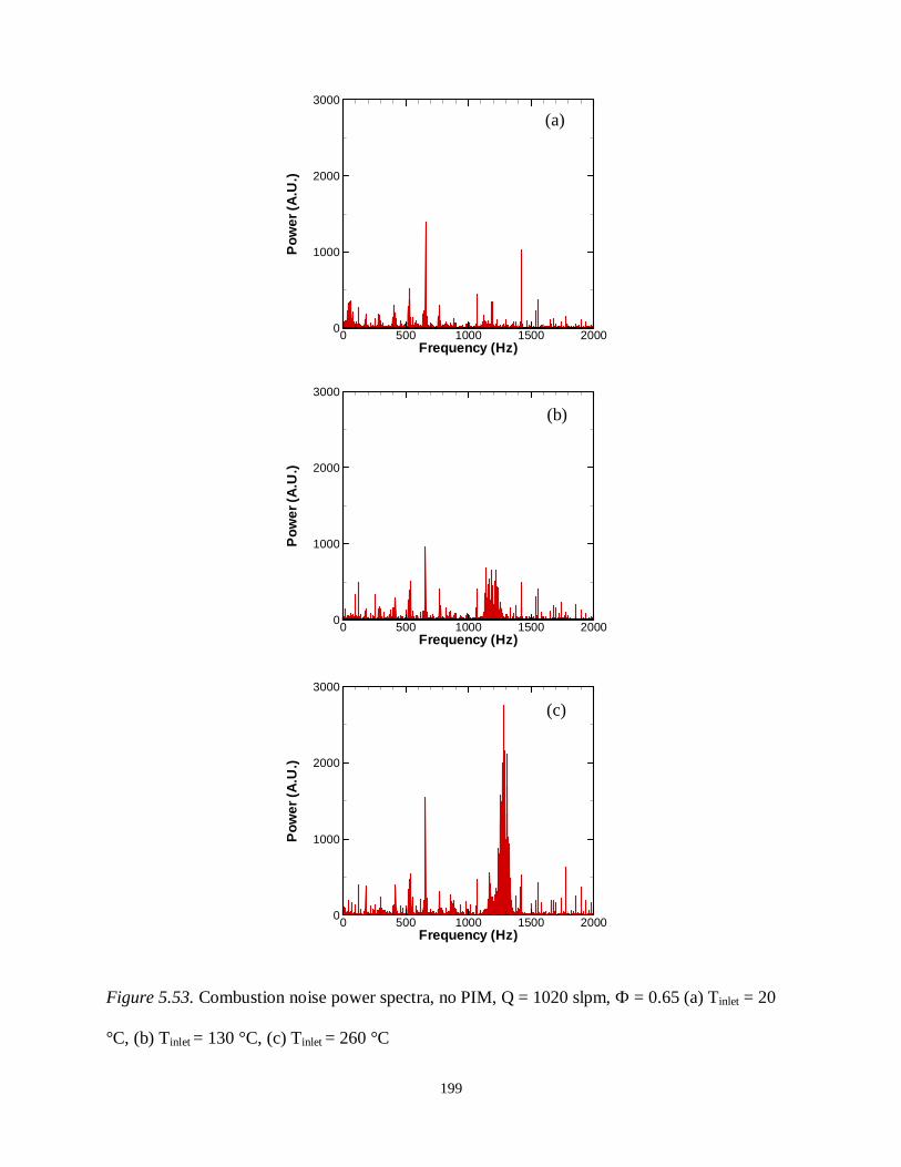
199
Figure 5.53. Combustion noise power spectra, no PIM, Q = 1020 slpm, Ф = 0.65 (a) Tinlet = 20
°C, (b) Tinlet = 130 °C, (c) Tinlet = 260 °C
(b)
(c)
(a)
Frequency (Hz)
Po
wer
(A.U
.)
0 500 1000 1500 20000
1000
2000
3000
Frequency (Hz)
Po
wer
(A.U
.)
0 500 1000 1500 20000
1000
2000
3000
Frequency (Hz)
Po
wer
(A.U
.)
0 500 1000 1500 20000
1000
2000
3000
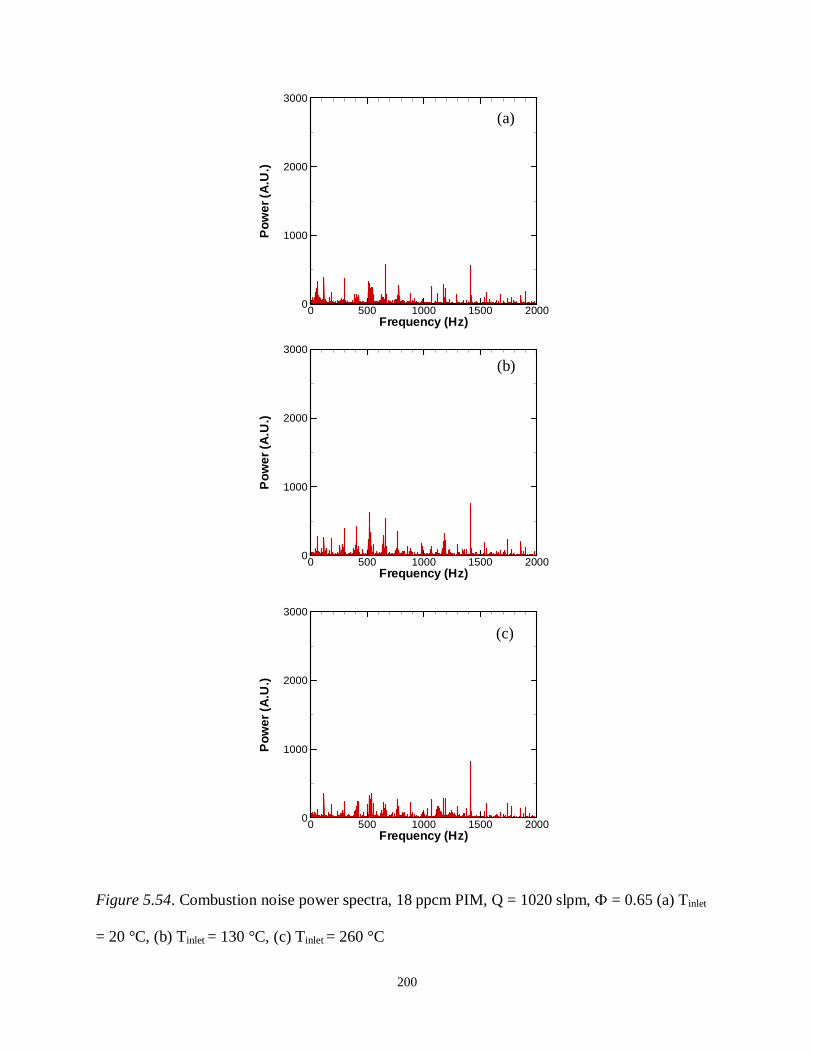
200
Figure 5.54. Combustion noise power spectra, 18 ppcm PIM, Q = 1020 slpm, Ф = 0.65 (a) Tinlet
= 20 °C, (b) Tinlet = 130 °C, (c) Tinlet = 260 °C
(b)
(c)
(a)
Frequency (Hz)
Po
wer
(A.U
.)
0 500 1000 1500 20000
1000
2000
3000
Frequency (Hz)
Po
wer
(A.U
.)
0 500 1000 1500 20000
1000
2000
3000
Frequency (Hz)
Po
wer
(A.U
.)
0 500 1000 1500 20000
1000
2000
3000
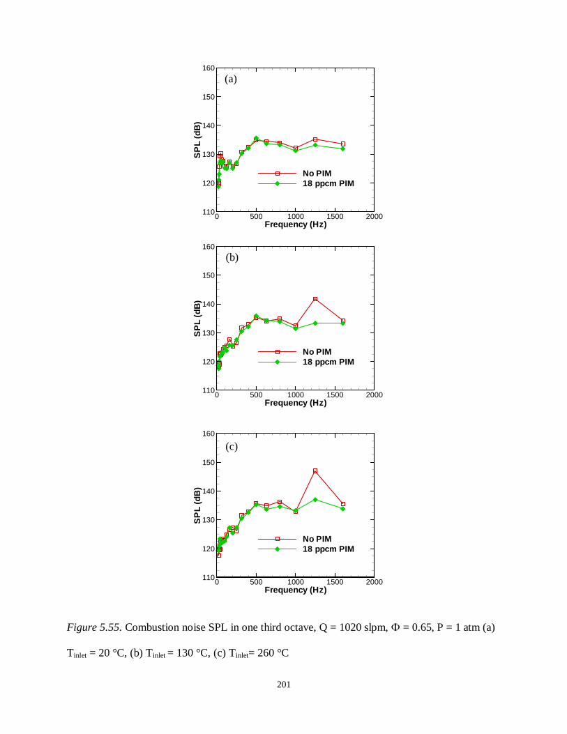
201
Figure 5.55. Combustion noise SPL in one third octave, Q = 1020 slpm, Ф = 0.65, P = 1 atm (a)
Tinlet = 20 °C, (b) Tinlet = 130 °C, (c) Tinlet= 260 °C
(b)
(c)
(a)
Frequency (Hz)
SP
L(d
B)
0 500 1000 1500 2000110
120
130
140
150
160
No PIM18 ppcm PIM
Frequency (Hz)
SP
L(d
B)
0 500 1000 1500 2000110
120
130
140
150
160
No PIM18 ppcm PIM
Frequency (Hz)
SP
L(d
B)
0 500 1000 1500 2000110
120
130
140
150
160
No PIM18 ppcm PIM
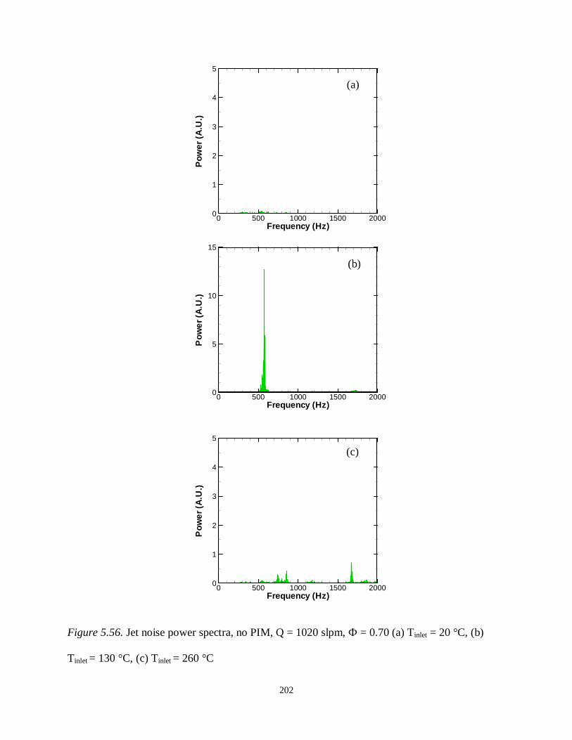
202
Figure 5.56. Jet noise power spectra, no PIM, Q = 1020 slpm, Ф = 0.70 (a) Tinlet = 20 °C, (b)
Tinlet = 130 °C, (c) Tinlet = 260 °C
(b)
(c)
(a)
Frequency (Hz)
Po
wer
(A.U
.)
0 500 1000 1500 20000
1
2
3
4
5
Frequency (Hz)
Po
we
r(A
.U.)
0 500 1000 1500 20000
1
2
3
4
5
Frequency (Hz)
Po
we
r(A
.U.)
0 500 1000 1500 20000
5
10
15

203
Figure 5.57. Jet noise power spectra, 18 ppcm PIM, Q = 1020 slpm, Ф = 0.70 (a) Tinlet = 20 °C,
(b) Tinlet = 130 °C, (c) Tinlet = 260 °C
(b)
(c)
(a)
Frequency (Hz)
Po
wer
(A.U
.)
0 500 1000 1500 20000
0.2
0.4
0.6
0.8
1
Frequency (Hz)
Po
we
r(A
.U.)
0 500 1000 1500 20000
0.2
0.4
0.6
0.8
1
Frequency (Hz)
Po
we
r(A
.U.)
0 500 1000 1500 20000
0.2
0.4
0.6
0.8
1

204
Figure 5.58. Jet noise SPL in one third octave, Q = 1020 slpm, Ф = 0.70, P = 1 atm (a) Tinlet = 20
°C, (b) Tinlet = 130 °C, (c) Tinlet = 260 °C
(b)
(c)
(a)
Frequency (Hz)
SP
L(d
B)
0 500 1000 1500 200060
70
80
90
100
110
120
130
No PIM18 ppcm PIM
Frequency (Hz)
SP
L(d
B)
0 500 1000 1500 200060
70
80
90
100
110
120
130
No PIM, location 118 ppcm PIM
Frequency (Hz)
SP
L(d
B)
0 500 1000 1500 200060
70
80
90
100
110
120
130
No PIM18 ppcm PIM
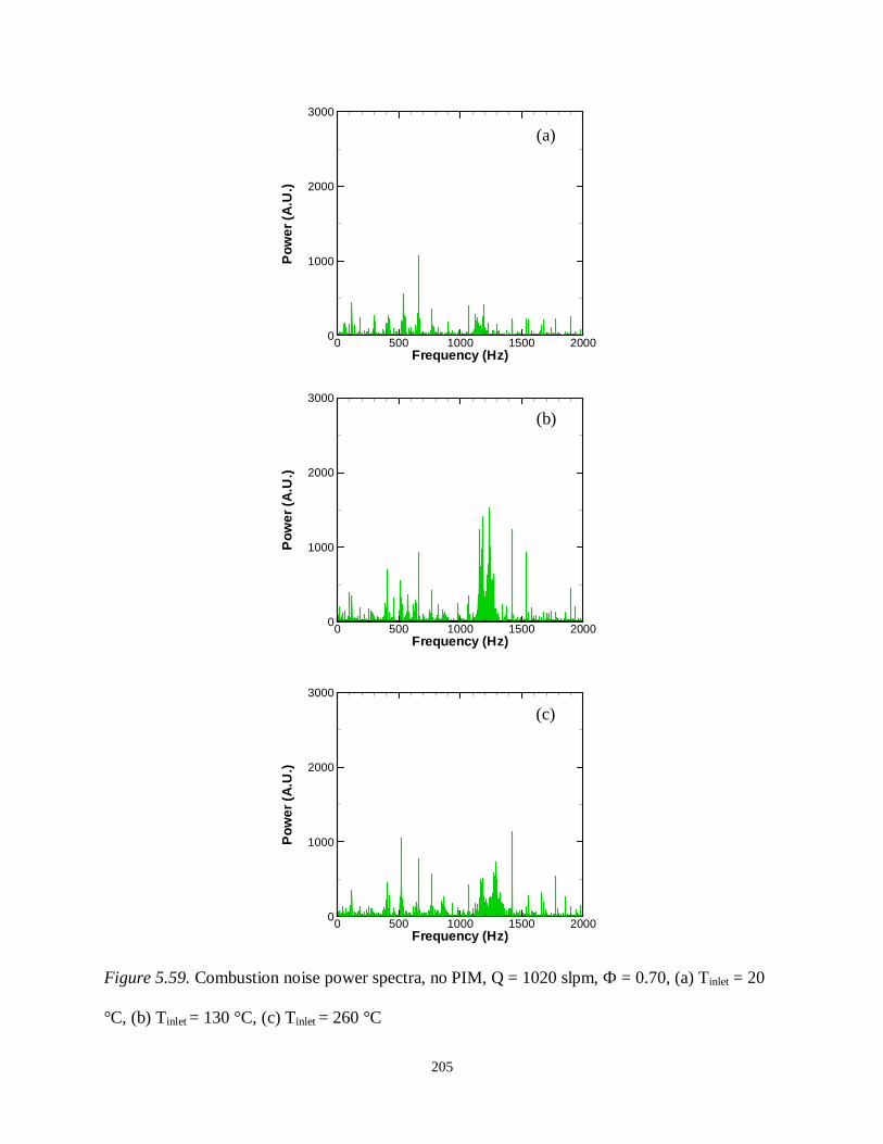
205
Figure 5.59. Combustion noise power spectra, no PIM, Q = 1020 slpm, Ф = 0.70, (a) Tinlet = 20
°C, (b) Tinlet = 130 °C, (c) Tinlet = 260 °C
(b)
(c)
(a)
Frequency (Hz)
Po
wer
(A.U
.)
0 500 1000 1500 20000
1000
2000
3000
Frequency (Hz)
Po
wer
(A.U
.)
0 500 1000 1500 20000
1000
2000
3000
Frequency (Hz)
Po
wer
(A.U
.)
0 500 1000 1500 20000
1000
2000
3000

206
Figure 5.60. Combustion noise power spectra, 18 ppcm PIM, Q = 1020 slpm, Ф = 0.70 (a) Tinlet
= 20 °C, (b) Tinlet = 130 °C, (c) Tinlet = 260 °C
(b)
(c)
(a)
Frequency (Hz)
Po
wer
(A.U
.)
0 500 1000 1500 20000
1000
2000
3000
Frequency (Hz)
Po
wer
(A.U
.)
0 500 1000 1500 20000
1000
2000
3000
Frequency (Hz)
Po
wer
(A.U
.)
0 500 1000 1500 20000
1000
2000
3000
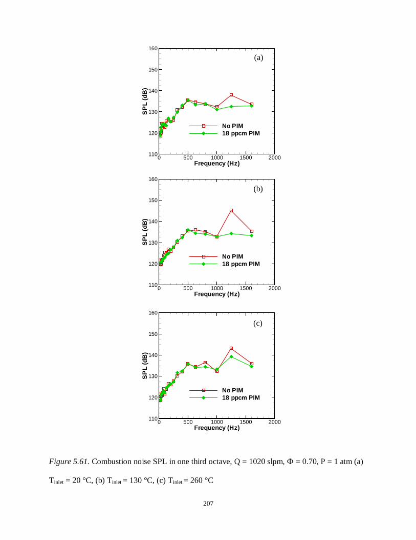
207
Figure 5.61. Combustion noise SPL in one third octave, Q = 1020 slpm, Ф = 0.70, P = 1 atm (a)
Tinlet = 20 °C, (b) Tinlet = 130 °C, (c) Tinlet = 260 °C
(b)
(c)
(a)
Frequency (Hz)
SP
L(d
B)
0 500 1000 1500 2000110
120
130
140
150
160
No PIM18 ppcm PIM
Frequency (Hz)
SP
L(d
B)
0 500 1000 1500 2000110
120
130
140
150
160
No PIM18 ppcm PIM
Frequency (Hz)
SP
L(d
B)
0 500 1000 1500 2000110
120
130
140
150
160
No PIM18 ppcm PIM
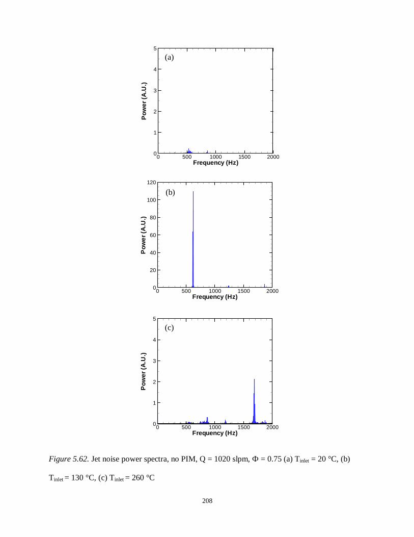
208
Figure 5.62. Jet noise power spectra, no PIM, Q = 1020 slpm, Ф = 0.75 (a) Tinlet = 20 °C, (b)
Tinlet = 130 °C, (c) Tinlet = 260 °C
Frequency (Hz)
Po
wer
(A.U
.)
0 500 1000 1500 20000
1
2
3
4
5
Frequency (Hz)
Po
we
r(A
.U.)
0 500 1000 1500 20000
20
40
60
80
100
120
(b)
(c)
(a)
Frequency (Hz)
Po
wer
(A.U
.)
0 500 1000 1500 20000
1
2
3
4
5

209
Figure 5.63. Jet noise power spectra, 18 ppcm PIM, Q = 1020 slpm, Ф = 0.75 (a) Tinlet = 20 °C,
(b) Tinlet = 130 °C, (c) Tinlet = 260 °C
(b)
(c)
(a)
Frequency (Hz)
Po
wer
(A.U
.)
0 500 1000 1500 20000
0.2
0.4
0.6
0.8
1
Frequency (Hz)
Po
we
r(A
.U.)
0 500 1000 1500 20000
0.2
0.4
0.6
0.8
1
Frequency (Hz)
Po
we
r(A
.U.)
0 500 1000 1500 20000
0.2
0.4
0.6
0.8
1

210
Figure 5.64. Jet noise SPL in one third octave, Q = 1020 slpm, Ф = 0.75, P = 1 atm (a) Tinlet = 20
°C, (b) Tinlet=130 °C, (c) Tinlet=260 °C
(b)
(c)
(a)
Frequency (Hz)
SP
L(d
B)
0 500 1000 1500 200060
70
80
90
100
110
120
130
No PIM18 ppcm PIM
Frequency (Hz)
SP
L(d
B)
0 500 1000 1500 200060
70
80
90
100
110
120
130
No PIM18 ppcm PIM
Frequency (Hz)
SP
L(d
B)
0 500 1000 1500 200060
70
80
90
100
110
120
130
No PIM18 ppcm PIM

211
Figure 5.65. Combustion noise power spectra, no PIM, Q = 1020 slpm, Ф = 0.75 (a) Tinlet = 20
°C, (b) Tinlet = 130 °C, (c) Tinlet = 260 °C
(b)
(c)
(a)
Frequency (Hz)
Po
wer
(A.U
.)
0 500 1000 1500 20000
80000
160000
240000
Frequency (Hz)
Po
wer
(A.U
.)
0 500 1000 1500 20000
1000
2000
3000
Frequency (Hz)
Po
wer
(A.U
.)
0 500 1000 1500 20000
1000
2000
3000

212
Figure 5.66. Combustion noise power spectra, 18 ppcm PIM, Q = 1020 slpm, Ф = 0.75 (a) Tinlet
= 20 °C, (b) Tinlet = 130 °C, (c) Tinlet = 260 °C
(b)
(c)
(a)
Frequency (Hz)
Po
wer
(A.U
.)
0 500 1000 1500 20000
1000
2000
3000
Frequency (Hz)
Po
wer
(A.U
.)
0 500 1000 1500 20000
1000
2000
3000
Frequency (Hz)
Po
wer
(A.U
.)
0 500 1000 1500 20000
1000
2000
3000
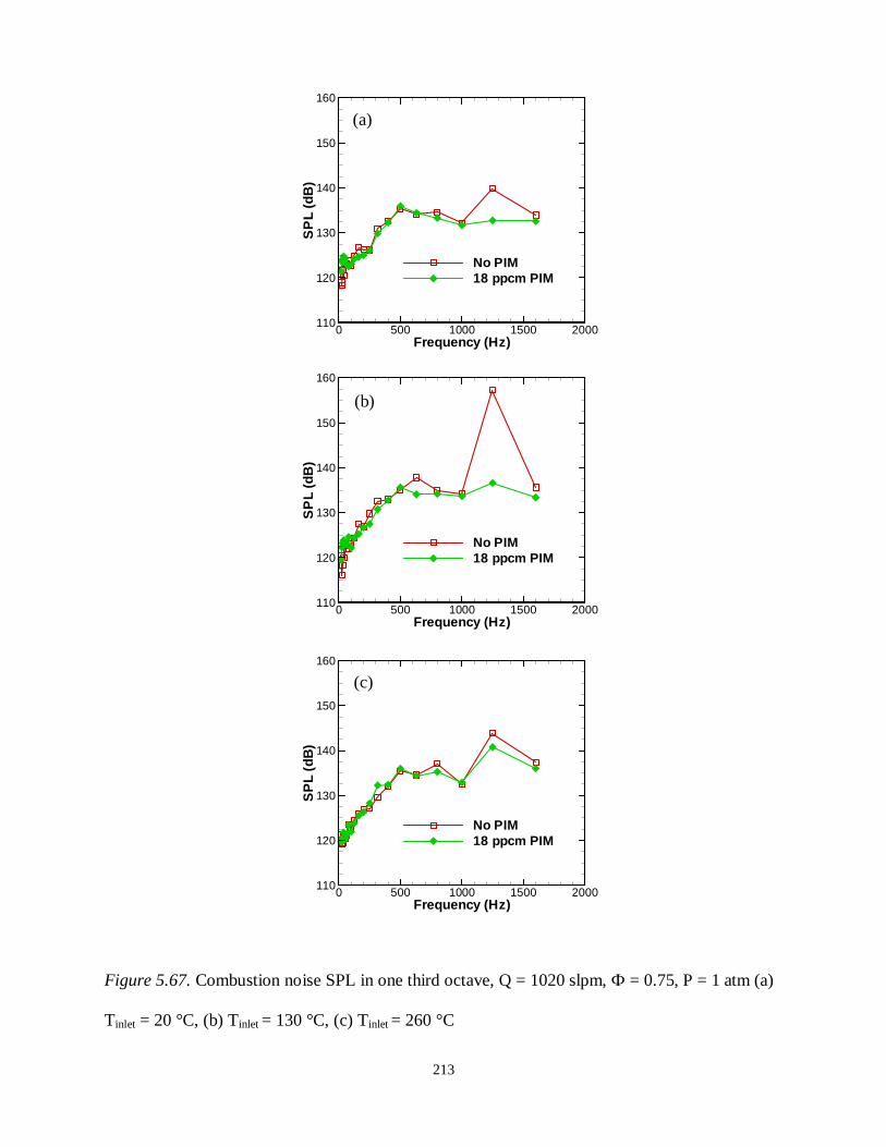
213
Figure 5.67. Combustion noise SPL in one third octave, Q = 1020 slpm, Ф = 0.75, P = 1 atm (a)
Tinlet = 20 °C, (b) Tinlet = 130 °C, (c) Tinlet = 260 °C
(b)
(c)
(a)
Frequency (Hz)
SP
L(d
B)
0 500 1000 1500 2000110
120
130
140
150
160
No PIM18 ppcm PIM
Frequency (Hz)
SP
L(d
B)
0 500 1000 1500 2000110
120
130
140
150
160
No PIM18 ppcm PIM
Frequency (Hz)
SP
L(d
B)
0 500 1000 1500 2000110
120
130
140
150
160
No PIM18 ppcm PIM

214
Figure 5.68. Pressure drop measurements for restricted top experiments, P = 1 atm (a) no PIM
(b) 18 ppcm PIM
Φ
∆P
(KP
a)
0.65 0.7 0.750
5
10
15
20
25
Tinlet = 20 oCTinlet = 130 oCTinlet = 260 oC
Φ
∆P
(KP
a)
0.65 0.7 0.750
5
10
15
20
25
Tinlet = 20 oCTinlet = 130 oCTinlet = 260 oC
(b)
(a)

215
Figure 5.69. Schematic diagram of nozzle for restricted flow experiments
Dimensions in cm
Direction of flow
3.8
1.9
2.9
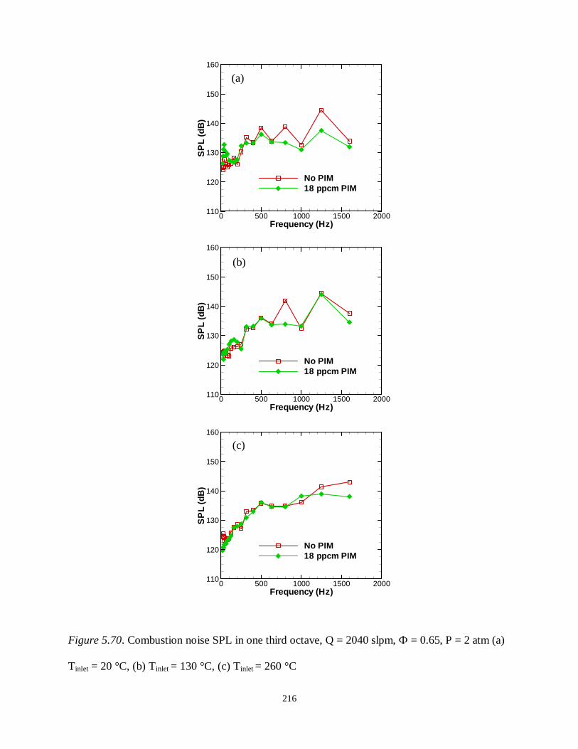
216
Figure 5.70. Combustion noise SPL in one third octave, Q = 2040 slpm, Ф = 0.65, P = 2 atm (a)
Tinlet = 20 °C, (b) Tinlet = 130 °C, (c) Tinlet = 260 °C
(b)
(c)
(a)
Frequency (Hz)
SP
L(d
B)
0 500 1000 1500 2000110
120
130
140
150
160
No PIM18 ppcm PIM
Frequency (Hz)
SP
L(d
B)
0 500 1000 1500 2000110
120
130
140
150
160
No PIM18 ppcm PIM
Frequency (Hz)
SP
L(d
B)
0 500 1000 1500 2000110
120
130
140
150
160
No PIM18 ppcm PIM

217
Figure 5.71. Combustion noise SPL in one third octave, Q = 2040 slpm, Ф = 0.70, P = 2 atm (a)
Tinlet = 20 °C, (b) Tinlet = 130 °C, (c) Tinlet = 260 °C
(b)
(c)
(a)
Frequency (Hz)
SP
L(d
B)
0 500 1000 1500 2000110
120
130
140
150
160
No PIM18 ppcm PIM
Frequency (Hz)
SP
L(d
B)
0 500 1000 1500 2000110
120
130
140
150
160
No PIM18 ppcm PIM
Frequency (Hz)
SP
L(d
B)
0 500 1000 1500 2000110
120
130
140
150
160
No PIM18 ppcm PIM
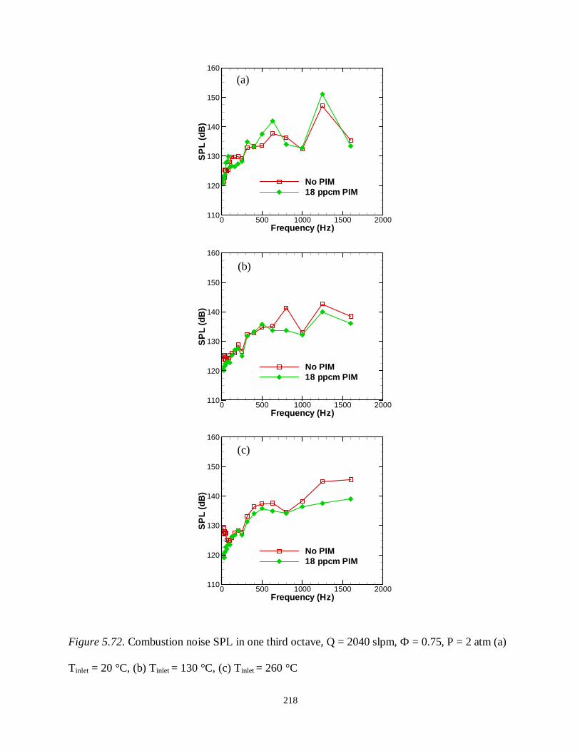
218
Figure 5.72. Combustion noise SPL in one third octave, Q = 2040 slpm, Ф = 0.75, P = 2 atm (a)
Tinlet = 20 °C, (b) Tinlet = 130 °C, (c) Tinlet = 260 °C
(b)
(c)
(a)
Frequency (Hz)
SP
L(d
B)
0 500 1000 1500 2000110
120
130
140
150
160
No PIM18 ppcm PIM
Frequency (Hz)
SP
L(d
B)
0 500 1000 1500 2000110
120
130
140
150
160
No PIM18 ppcm PIM
Frequency (Hz)
SP
L(d
B)
0 500 1000 1500 2000110
120
130
140
150
160
No PIM18 ppcm PIM

219
Figure 5.73. Pressure drop measurements for restricted top experiments, P = 2 atm (a) no PIM
(b) 18 ppcm PIM
Φ
∆P
(KP
a)
0.65 0.7 0.750
5
10
15
20
25
Tinlet = 20 oCTinlet = 130 oC
Φ
∆P
(KP
a)
0.65 0.7 0.750
5
10
15
20
25
Tinlet = 20 oCTinlet = 130 oCTinlet = 260 oC
(b)
(a)
220
CHAPTER 6
CONCLUSIONS AND RECOMMENDATIONS
6.1 Conclusions
In the present study, swirl stabilization mechanism is combined with porous inert media
for lean premixed combustion with the goal to reduce combustion generated noise without
affecting CO and NOx emissions. Gaseous fuel is used as a first step to eventually implement the
concept in a liquid fuel combustor. The approach involves passive control of the flow structures
that generate noise in combustion chamber. This approach can also mitigate combustion
instabilities that self-excite within the combustor. First, time-averaged numerical simulation of
non-reacting and reacting flows is performed to gain insight into the flow structure without and
with the porous insert. Next, an experimental investigation was conducted to determine impact of
PIM geometric parameters (such as ID, pore size) on sound pressure levels. Initially, experiments
were conducted at atmospheric pressure, and relatively low reactant flow rates and low inlet air
temperatures. Results were used to identify combustion modes and PIM configurations that are
most beneficial for noise reduction. Next, a laboratory facility was designed and developed to
conduct combustion experiments at high reactant flow rate, high inlet air temperature, and high
operating pressures. Details of the design, installation and operation of this laboratory facility are
presented. The facility was utilized for the next series of experiments to more closely simulate
typical gas turbines operating conditions, i.e., high reactant flow rate, high inlet air temperature

221
and high pressure. PIM configurations optimized in previous study were utilized. Following are
the main conclusions:
• Numerical model shows qualitative agreement with experimentally obtained data for
reacting and non-reacting flows. The study shows that flow inside combustion chamber is
redistributed: porous insert eliminates the corner recirculation zone, vertically orients the
gaseous flame zone, intensifies the central recirculation zone, maintains the swirling
effect imparted by the swirl injector, and creates a more uniform flow distribution at
downstream locations. These features can be expected to improve the noise and
instability performance of combustor.
• Experimental study identified interior and surface modes of swirl-stabilized combustion
with porous insert. Equivalence ratio, reactant flow rate, and PIM geometric parameters
such as ID and pore size determine the combustion mode. Surface combustion mode is
desirable, while interior combustion must be avoided to achieve low SPLs. Lower pore
density (<18 ppcm) resulted in undesired interior combustion mode and increased SPL. A
divergent porous insert with pore density of 18 ppcm was found to reduce the total SPL
by up to 14 dB. NOx and CO emissions were not adversely affected by the porous insert.
• A new laboratory facility for combustion experiments at high reactant flow rate, high
inlet air temperature, and high operating pressure was developed. A combustor
experimental apparatus was designed and fabricated to operate at pressure up to 10 atm.
The combustor designed consisted of different size nozzle to choke the flow downstream
of the combustion chamber. The experimental apparatus was demonstrated to operate
with air flow rate up to 3 kg/min, Tinlet = 260 °C and pressure of up to 4 atm.

222
• Experiments were conducted in the new facility at a higher operating pressure, high
reactant flow rate, and high inlet air temperature, to more closely simulate gas turbine
engine operating condition. Porous inserts of 18 and 32 ppcm were used. Jet noise and
combustion noise were measured independently. Pressure drop across swirl injector and
combustor was also measured. Results show that porous insert reduces both jet noise and
combustion noise. Furthermore, combustion instability present without porous insert was
mitigated by use of PIM. Porous insert effectively attenuated heat release fluctuations
associated with turbulent nature of flame. This result was obtained only with combustion
occurring on the surface of the porous insert. Difference between PIM of 18 and 32 ppcm
is not significant. Cases with no instabilities also showed a reduction in the total SPL
with use of porous insert. Highest pressure drop registered pertained highest inlet
temperature, and PIM did not affect CO or NOx emissions or pressure drop across the
combustor.
6.2 Recommendations
Recommendations for future scope and improvements of current work are listed below:
• A time dependent numerical model is recommended. Flow field, pressure field and heat
release fluctuations are of particular interest. A numerical study with porous insert of
diffuser shaped inside wall is recommended. Model can be extended to predict acoustic
behavior of the combustor.
• A study of swirl number effect on SPL. Swirl number can affect turbulence intensity in
corner recirculation zone, which in turn affects pressure fluctuations. Also, location of
swirler with respect to dump plane impacts total SPL by creating recirculation zones
223
within the premixer tube. Thus, an investigation of swirler parameters, such as swirl
number and location within the premixer, is recommended.
• Experiments with longer porous inserts (in the axial direction) at elevated flow rate. It
was observed that high reactant velocities tend to stretch reaction zone in the axial
direction of the combustor. Thus a longer porous insert could enhance heat transfer and
acoustic dissipation inside combustion chamber for these cases.
• An experimental investigation that combines PIM with liquid fuel combustion under
optimum atomization operating conditions is recommended.
• A more durable and flexible traversing system/emission probe to facilitate mounting and
emission measurements. Quartz holding mechanism that is more durable and reliable, and
a safe means to easily remove/mount combustor reducer apparatus.
• For safety, automation of an ignition system that can be remotely activated is
recommended.
• An automated control of combustion/cooling air split by merging air and fuel control
software interfaces is recommended.
• Redirect cooling air jets inside enclosure to improve cooling of windows.

224
REFERENCES
Agrawal, A.K., S. Vijaykant, (2010). Passive Noise Attenuation System. U.S. Patent Application 20100059311, The University of Alabama.
B. F. Magnussen and B. H. Hjertager, (1976). On mathematical models of turbulent combustion
with special emphasis on soot formation and combustion. Proceedings of the Combustion Institute, vol. 16, pp. 719-729.
Bussman, W., and Jayakaran, J., (2001). Noise. The John Zink Combustion Handbook, CRC
Press, New York. Bertoli, C., D’Alessio, J., Del Giacomo, N., Lazzaro, M., Massoli, P., and Moccia, V., (2000).
Running Light-Duty DI Diesel Engines with Wood Pyrolysis Oil. SAE Paper 200-01-2975.
Broda, J. C., Seo, S., Santoro, R. J., Shirhattikar, G., and Yang, V., (1998). An Experimental
Study of Combustion Dynamics of a Premixed Swirl Injector. Proceedings of the Combustion Institute, Pittsburgh, PA, vol. 27, pp. 1849-1856.
Cheng, R.K., Yegian, D.T., Miyasato, M.M., Samuelsen, G.S., Pellizzari, R., and Benson, C.,
(2000). Scaling and Development of Low-Swirl Burners for Low-Emission Furnaces and Boilers. Proceedings of the Combustion Institute, vol. 28, pp. 1305-1313.
Chiaramonti, D., Oasmaa, A., and Solantausta, Y., (2006), Fast Pyrolysis Oil for Power
Generation. ASME Paper GT2006-90245.Chigier, N.A., and Beer, J.M., (1964). Velocity and static pressure distributions in swirling air jets issuing from annular and divergent nozzles. Journal of Basic Engineering, vol. 86, n. 4, pp. 788-796.
Choi, G., Tanahashi, M., Miyauchi, T., (2005). Control of Oscillating Combustion and Noise
Based on Local Flame Structure. Proceedings of the Combustion Institute, vol. 30, pp. 1807-1814.
Czernik, S., and Bridgewater, A.V., (2004). Overview of Applications of Biomass Fast Pyrolysis
Oil. Energy and Fuels, vol. 18, pp. 590-598.
225
Damstedt, B., Pederson, J.M., Hansen, D., Knighton, T., Jones, J., Christensen, C., Baxter, L., and Tree, D., (2007). Biomass Cofiring Impacts on Flame Structure and Emissions. Proceedings of the Combustion Institute, doi:10.1016/j.proci.2006.07.155.
De La Torre Ugarte, D.G., (2003). The Economic Impact of Bioenergy Crop Production on U.S.
Agriculture. US Department of Agriculture and Department of Energy. Agricultural Economic Report No. 816 (www.usda.gov/oce/reports/energy/AER816Bi.pdf).
Demirbas, A., (2004). Combustion Characteristics of Different Biomass Fuels. Progress in
Energy and Combustion Science, vol. 30, pp. 219-230. Duchaine, P., Zimmer, L., Schuller, T., (2009). Experimental Investigation of Mechanisms of
Sound Production by Partially Premixed Flames. Proceedings of the Combustion Institute, vol. 32, pp. 1027-1034.
Fernandez-Pello, A.C., (2002). Micropower Generation Using Combustion: Issues and
Approaches. Proceedings of the Combustion Institute, vol. 29, pp. 883 – 899. Flemming, F., Olbrit, C., Wegner, B., Sadiki, A., Janicka, J., Bake, F., Michael, U., Lehmann,
B., Rohle, I., (2005). Analysis of Unsteady Motion with Respect to Noise Sources in a Gas Turbine Combustor: Isothermal Flow Case. Flow, Turbulence and Combustion, vol. 75, pp. 3-27.
Grinstein, F. F., and Fureby, C., (2005). LES Studies of the Flow in a Swirl Combustor.
Proceedings of the Combustion Institute, Pittburgh, PA, vol. 30, pp. 1791-1798. Gupta, A.K., Lilley, D.G., and Syred N., (1984). Swirl Flows. Abacus Press, Tunbridge Wells,
England. Hirsch, C., Wasle, J., Winkler, A., Sattelmayer, T., (2007). A Spectral Model for the Sound
Pressure from Turbulent Premixed Combustion. Proceedings of the Combustion Institute, vol. 31, pp. 1435-1441.
Howell, J.R., Hall, M.J., and Ellzey, J.L., (1996). Combustion of Hydrocarbon Fuels within
Porous Inert Media. Progress in Energy and Combustion Science, vol. 22, n. 2, pp. 121-145.
Huang, Y., Sung, H. G., Hsieh, S. Y. and Yang, V., (2003). Large Eddy Simulation of Combustion Dynamics of Lean-Premixed Swirl-Stabilized Combustor. Journal of Propulsion and Power, vol. 19, pp. 782-794.
Ikura, M., Stanciulescu, M., and Hogan, E., (2003). Emulsification of Pyrolysis Oil Derived
Biooil in Diesel Fuel. Biomass and BioEnergy, vol. 24, pp. 221-232. Jayasuria, J., Manrique, A., Fakhrai, R., Fredriksson, J., and Fransson, T., (2006). Gasified
Biomass Fuelled Gas Turbine: Combustion Stability and Selective Catalytic Oxidation of Fuel-Bound Nitrogen. ASME Paper GT2006-90988.

226
Kee. R.J., Rupley, F.M., Miller, J.A. Chemkin II: A FORTRAN Chemical Kinetics Package for the Analysis of Gas Phase Chemical Kinetics” Sandia Report SAND89-809B-UC-706.
Lieuwen, T., McDonnell, V., Petersen, E., and Santavicca, D., (2006). Fuel Flexibility Influences
on Premixed Combustor Blowout, Flashback, Autoignition, and Stability. ASME Paper GT2006-90770.
Lieuwen, T., Yang, V., (2005). Combustion Instabilities in Gas Turbine Engines. Progress in
Astronautics and Aeronautics, vol. 210, Arlington, Texas. Littlejohn, D., Cheng, R.K., (2007). Laboratory Study of Premixed H2-Air & H 2-N2-Air flames
in a Low-Swirl Injector for Ultra-Low Emissions Gas Turbines. ASME Paper GT2007-27512.
Littlejohn, D., Majeski, M.J., Tonse, S., Castaldini, C., and Cheng, R.K., (2002). Laboratory
Investigation of an Ultralow NOx Premixed Combustion Concept for Industrial Boilers. Proceedings of the Combustion Institute, vol. 29, pp. 1115-1121.
Lee, J.G., Santavicca, D.A., (2003). Experimental Diagnostics for the Study of Combustion
Instabilities in Lean Premixed Combustors. Journal of Propulsion and Power, vol. 19, n. 5, pp. 735-750.
Lupandin, V., Thamburaj, R., and Nikolayev, A., (2005). Test Results of the OGT2500 Gas
Turbine Engine Running on Alternative Fuels: Biooil, Ethanol, Biodiesel, and Crude Oil. ASME Paper GT2005-68488.
Marbach, T.L., and Agrawal, A.K., (2006). Computational Study of a Mesoscale Combustor
Using Porous Inert Media for Heat Recirculation. AIAA Paper 2006-1443. Marbach, T.L., and Agrawal, A.K., (2005). Experimental Study of Surface and Interior
Combustion Using Composite Porous Inert Media. Journal of Engineering for Gas Turbines and Power, vol. 127, n. 2, p 307 – 313.
Marbach, T.L., Sadasivuni, V., and Agrawal, A.K., (2007). Investigation of a Miniature
Combustor Using Porous Media Surface Stabilized Flame. Combustion Science and Technology, vol. 179, issue 9, pp. 1901-1922.
Mohan, D., Pittman, C.U., Steele, P.H., (2006). Pyrolysis of Wood/Biomass for Biooil: A Critical Review. Energy and Fuels, vol. 20, pp. 848-889.
Moriconi, A., Quirini, C., Moriconi, D., and Moriconi, E., (2005). Gas Turbine Fed by Gas
Produced from Biomass Pyrolysis. ASME Paper GT2005-69032. Nazeer, W.A., Smith, K.O., Sheppard, P., Cheng, R.K., and Littlejohn, D., (2006). Full Scale
Testing of a Low Swirl Fuel Injector Concept for Ultra-Low NOx Gas Turbine Combustion Systems. ASME Paper GT2006-90150.

227
Noiray, N., Durox, D., Schuller, T., Candel, S., (2009). Dynamic Phase Converter for Passive Control of Combustion Instabilities. Proceedings of the Combustion Institute, vol. 32, pp. 3163-3170.
Oasmaa, A., and Czernik, S., (1999). Fuel Oil Quality of Biomass Pyrolysis Oils – State of the
Art for the End Users. Energy and Fuels, vol. 13, pp. 914-921. Putnam, A.A., (1978). Combustion Noise in Industrial Burners. Noise Control Engineering,
vol.7, issue 1, pp. 24-34. Rayleigh, J.S.W., (1945). The Theory of Sound, vol. 2, Dover, New York. R. Rajaram, J. Gray, T. Lieuwen, (2006). Premixed Combustion Noise Scaling: Total Power and
Spectra. AIAA paper 2006-2612. Richards, G.A., McMillian, M.M., Gemmen, R.S., Rogers, W.A., and Cully, S.R., (2001). Issues
for Low-Emission, Fuel-Flexible Power Systems. Progress in Energy and Combustion Science, vol. 27, pp. 141-169.
Richards, G.A., Straub, D.L., (2003). Passive Control of Combustion Dynamics in Stationary
Gas Turbines. Journal of Propulsion and Power, vol. 19, n. 5, pp. 795-810. Sequera, D., and Agrawal, A.K., (2007). Emissions and Acoustics Measurements in a Low-Swirl
Burner. AIAA Paper 2007-1347. Smagorinsky, J., (1963). General Circulation Experiments with the Primitive Equations I. The
Basic Experiment. Month. Wea. Rev., 91:99-164. Stone, C., and Menon, S., (2002). Swirl Control of Combustion Instabilities in a Gas Turbine
Combustor. Proceedings of the Combustion Institute, Pittsburgh, PA, vol. 29, pp. 155-160.
Strahle, W.C., (1978). Combustion Noise. Progress in Energy and Combustion Science, vol. 4,
issue 3, pp. 157–176.
Strenziok, R., Hansen, U., and Knunster, H., (2001). Combustion of Biooil in a Gas Turbine. Progress in Thermochemical Biomass Conversion, Bridgwater, A.V., (Ed.), Blackwell Science, Oxford, pp. 1452-1458.
Schwarz, A., Janicka, J., (2009). Combustion Noise, Springer-Verlag Berlin Heidelgerg,
Germany. Tiribuzi, S., (2008). CFD Simulation of Noise in Gas Turbine Combustors by Means of
Turbulence Refluctuation Method. Proceedings of the ASME Turbo Expo, vol. 3, pp. 113-124.

228
Trimis, D., and Durst, F., (1996). Combustion in a Porous Medium – Advances and Applications. Combustion Science and Technology, vol. 121, pp. 153-168.
Turns, Stephen, (2000). An Introduction to Combustion: Concepts and Applications. McGraw-
Hill 2nd Edition. V. Zimont, (2000). Gas Premixed Combustion at High Turbulence. Turbulent Flame Closure
Model Combustion Model. Experimental Thermal and Fluid Science, vol. 21, pp. 179-186.
V. L. Zimont and A. N. Lipatnikov, (1995). A Numerical Model of Premixed Turbulent
Combustion of Gases. Chem. Phys. Report, vol. 14, n. 7, pp. 993-1025. V. Zimont, W. Polifke, M. Bettelini, and W. Weisenstein, (1998). An Efficient Computational
Model for Premixed Turbulent Combustion at High Reynolds Numbers Based on a Turbulent Flame Speed Closure. Journal of Gas Turbines Power, vol. 120, pp. 526-532.
Vijaykant, S., Agrawal, A.K., and Stewart, Timothy, (2008). Combustion Noise Reduction Using
Porous Inert Medium. AIAA Paper 2008-1057.
Waitz, I.A., Gauba, G., and Tzeng, Y.S., (1998). Combustors for Micro-gas Turbine Engines. Journal of Fluids Engineering, vol. 120, pp. 109 – 117.
Wicksall, D.M., and Agrawal, A.K., (2005). Influence of Hydrogen Addition on Flow Structure
in Confined Swirling Methane Flame. AIAA Journal of Propulsion and Power, vol. 21, n. 1, pp. 16-24.
William E. Harrison, Clean Fuel Initiative,
www.cffs.uky.edu/C1/2002meeting/WPAFBharrison.pdf Wong, T. and Agrawal, A., (2006). Quantitative Measurement in an Unsteady Flame Using
High-Speed Rainbow Schlieren Deflectometry. Measurement Science and Technology, vol. 17, pp. 1503-1510.
Yegian, D.T., and Cheng, R.K., (1998). Development of a Lean Premixed Low-Swirl Burner for
Low NOx Practical Applications. Combustion Science and Technology, vol. 139, pp. 207-227.

229
APPENDIX A
COMBUSTION PERFORMANCE OF LIQUID BIO-FUELS IN A SWIRL-STABILIZED BURNER
Background
Unlike non-renewable fossil fuels, the CO2 emitted from the combustion of biofuels is
recycled in the environment through future plant growth. A recent study projects that with
relatively modest changes in land use and agricultural and forestry practices, an annual supply of
1.36 billion dry tons of biomass could be available for large-scale biofuel production in the
United States by the mid-21st century, while still meeting demands for forestry products, food
and fiber (De La Torre, 2003)
Biomass can be converted into solid, gaseous or liquid fuel depending upon the
conversion processes and economic factors. Several current biomass technologies are reviewed
in (Demirbas, 2004). Co-firing of biomass with coal is among the most cost effective
approaches (Damstedt, 2007). Since combustion of solid fuels results in higher emissions (e.g.,
soot and nitric oxides or NOx), liquid and/or gaseous fuels produced from biomass are likely to
become increasingly prevalent in the near term. Biomass can be gasified in air-blown or oxygen-
blown gasifier, followed by the cleanup of the product gas (known as synthetic gas or syngas)
containing carbon monoxide (CO) and hydrogen (H2) as the primary reactants. The biomass
syngas can serve as the fuel to generate power in a high-efficiency combined cycle power plant.
The combined cycle power plant integrated with the gasification system can operate
230
synergistically with biomass and/or coal as feedstock, since the syngas produced from
gasification of either of these sources (biomass or coal) contains the same reactive ingredients.
In contrast to biomass syngas requiring large-scale stationary operation, liquid biofuels
offer greater flexibility since the fuel can be transported easily. Liquid biofuels offer the
prospects of distributed generation, whereby the power is produced closer to the source without
hauling the bulky biomass to a distant central location. At present, ethanol and biodiesel are the
two commonly used liquid biofuels. However, the feedstocks for these fuels compete with the
food-chain crops. For example, virtually all of the ethanol produced in the US comes from corn
and biodiesel is produced by the transesterification of vegetable oils such as soybean oil. Thus, a
long-term strategy will require liquid fuels from biomass feedstocks such as wood and energy
crops that do not interfere with the food chain.
The biomass must undergo gasification or pyrolysis to produce the liquid fuel. Starting
with the biomass syngas, the well-known Fischer-Tropsch (FT) process can be used to produce
liquid biofuels of desired composition and physical characteristics. Although the FT process is
attractive to produce liquid biofuels for vehicular transportation (William, 2002), the fuels
produced by pyrolysis of biomass can be economic alternatives for power generation
applications. Pyrolysis is the thermal destruction of organic material in the absence of or limited
supply of oxygen (Damstedt, 2007). In fast pyrolysis, the thermal decomposition occurs at
moderate temperatures with a high heat transfer rate to the biomass particles and a short hot
vapor residence time in the reaction zone (Oasma, 1999; Czernik, 2004; Mohan, 2006). The
main product is the pyrolysis oil, also known as biooil, which is usually a dark-brown free-
flowing liquid with a distinctive smoky odor. Biooils have been successfully tested in diesel
engines and gas turbines (Strenziok, 2001; Bertoli, 2000; Lupandin, 2006), although

231
modifications to the fuel handling system can incur unacceptable financial cost. Thus, a near-
term strategy would be to emulsify biooil using fuels compatible with the fuel handling
equipment. Ikura et al. (2003) produced biooil emulsified with the diesel fuel. The cost for
producing emulsions with zero stratification increased with increasing amounts of biooil in the
diesel fuel.
The literature review shows few studies on combustion performance of liquid bio-fuels
for gas turbine applications. Thus, the primary objective of this study is to isolate the effects of
fuel composition and fluid dynamics on emissions from different liquid fuels in an atmospheric
pressure burner replicating typical features of a gas turbine combustor. The burner utilized a
commercial twin-fluid injector with primary air swirling around the injector. The fuels include
diesel, biodiesel, emulsified biooil, and diesel-biodiesel blends. Biooil emulsions were produced
using blends of biodiesel and diesel to increase the amount of biomass derived fuel in the final
product. The emulsified biooil produced in this manner is expected to require minimal
modifications to the fuel handling system. For fixed volume flow rates of fuel and air,
experiments were conducted by varying the airflow split between the injector and co-flow
swirler. Results include visual flame images, and axial and radial profiles of NOx and CO
concentrations at different operating conditions. In the following sections, the fuel preparation
steps and experimental setup details are outlined followed by results and discussions.
A.2 Fuel Preparation
As mentioned above, the fuels in this study included diesel, biodiesel, emulsified biooil,
and diesel-biodiesel blends. The diesel fuel used was of a commercial grade (No. 2 diesel fuel)
purchased from a local filling station. The biodiesel was supplied by Alabama Biodiesel

232
Corporation (Moundville, AL) and it was a soybean oil methyl ester (SME). Pyrolysis oil, also
known as, biooil (from hardwood) was provided by the National Renewable Energy Labortory
(NREL; Boulder, CO). It was a hot-vapor filtered biooil with very low ash content. The biooil
was approximately one-year old, and was not phase separated or treated with any viscosity
reducing agents. The NREL biooil composition is summarized below in Table A.1.
The emulsified biooil was formulated by mixing diesel, biooil and ‘surfactants’. The
‘surfactants’ used in this study was a blend of biodiesel, 2-ethyl-1-hexanol (an alcohol), and n-
octylamine. The latter two chemicals were purchased from Aldrich (Milwaukee, WI). The
emulsified fuel was produced by mixing diesel, biodiesel, biooil, alcohol, and amine using a high
shear (10,000 rpm) Oster blender (Boca Raton, FL). Mixing was done at room temperature and
pressure until an emulsified liquid was obtained in about 2 minutes. In this study, two types of
biodiesel (SME and 90% ethyl oleate hereafter referred to as SEE) were mixed with diesel by
gentle stirring to form diesel-biodiesel fuel blends. These blends are completely miscible over
all concentration ranges. Table A.2 summarizes the fuels used in this study.
The water content of each fuel was determined by a volumetric Aquastar Karl-Fischer
titrator (EM Science, Gibbstown, NJ) with Composite 5 solution as the titrant and anhydrous
methanol as the solvent. All measurements were made in triplicate and at 25oC. The water
content in the fuel blends is summarized below in Table A.3.

233
Table A.1
NREL Biooil Characteristics
Biooil Diesel* Biodiesel†
Moisture content (wt. %) 20.0
Ash (wt. %) 0.018
Elemental composition (wt. %)
Carbon 45.6 86.7 78.61
Hydrogen 7.6 13.5 11.99
Nitrogen 0.05 0.04 2.1‡
Sulfur 0.02 0.03 <0.004
Oxygen 46.8 9.38
* From Chiaramonti et al, 2006 † From Ikura et al, 2003. ‡ ppm.
Table A.2
Experimental Fuel Blends (Vol%)
Fuel Diesel Biodiesel
(SME+SEE)
Biooil Alcohol/
Amine
Diesel 100
Biodiesel (100 + 0)
Biooil 45 (30 + 0) 15 8/2
SOME 80 (20 + 0)
SOEE 80 (0 + 20)

234
Table A.3
Water Contents in the Fuel Blend
Fuel % w/w ± 3σ**
Diesel 0.021 ± .006
Biodiesel 0.10 ± .01
Biooil 0.27 ± .04
SOME 0.03 ± .01
SOEE 0.017 ± .004
BioOil (as received)† 22.9 ± 1.4
†Water content most likely increased during storage.
A.3 Experimental Setup
The test apparatus shown schematically in Figure A.1 consists of the combustor assembly
and the injector assembly. The primary air enters the system through a plenum filled with
marbles to breakdown the large vortical structures. The air passes through a swirler into the
mixing section, where the gaseous fuel is supplied during the startup. The reactant(s) enter the
combustor through a swirler used to improve the fuel-air mixing. Figure A.2 shows a schematic
diagram and a photograph of the combustor inlet section with the swirler.
The swirler had six vanes positioned at 28o to the horizontal. The theoretical swirl
number was 1.5, assuming that the flow exited tangentially from the swirler vanes. The bulk
axial inlet velocity of the primary air was 1.9 to 2.1 m/s, which resulted in Reynolds number
varying from 5960 to 6750. The liquid fuel is supplied from an injector with separate concentric
inlets for fuel and atomization air. The injector system runs through the plenum and the mixing

235
chamber. An O-ring within a sleeve is provided at the bottom of plenum to prevent any leakage.
The injector is a commercial air-blast atomizer (Delavan Siphon type SNA nozzle) and it creates
a swirling flow of atomizing air to breakdown the fuel jet. The injector details are shown in
Figure A.3. The combustor itself is a 8.0 cm ID and 46 cm long quartz tube. The combustor is
back-side cooled by natural convection.
The liquid fuel is supplied by a peristaltic pump with the range of flows rates from 2
ml/min to 130 ml/min in steps of 2 ml/min. The reported calibration error of the pump is +/-
0.25% of the flow rate reading. Viton tubes were used prevent any degradation of the fuel lines.
A 25 micron filter was used to prevent dirt and other foreign particles from clogging the injector.
The primary and atomizing air is supplied by an air compressor. The air passes through a
pressure regulator and a water trap to remove the moisture. Then, the air is split into primary air
supply and atomizing air supply lines. The primary air flow rate is measured by a laminar flow
element calibrated for 0 to 1000 liters per minute (lpm) of air. The pressure drop across the LFE
is measured by a differential pressure transducer. An absolute pressure transducer is used to
measure the pressure of air passing through the LFE. The flow rate measured by the LFE is
corrected for temperature and pressure as specified by the manufacturer. The atomizing air is
measured by calibrated mass flow meter.
The product gas was sampled continuously by a quartz probe (OD = 7.0 mm) attached to
a three-way manual traversing system. The upstream tip of the probe was tapered to 1 mm ID to
quench reactions inside the probe. The sample passed through an ice bath and water traps to
remove moisture upstream of the gas analyzers. The dry sample passed through electrochemical
analyzers to measure the concentrations of CO and NOx in ppm. The analyzer also measured
oxygen and carbon dioxide concentrations, which were used to cross-check the equivalence ratio

236
obtained from the measured fuel and air flow rates. The uncorrected emissions data on dry basis
are reported with measurement uncertainty of +/- 2 ppm.
The experiment was started by supplying the gaseous methane and then, igniting the
methane-air reactant mixtures in the combustor. Next, the liquid fuel flow rate was gradually
increased to attain the desired value, while the methane flow rate was slowly decreased to zero.
In this study, the volume flow rates of total air (primary + atomizing) and fuel were kept
constant, respectively, at 150 standard lpm and 12 ml/min. It could result in small variations in
the amount of heat-released since the heating value of fuels is different. The combustion
performance is strongly dependent upon the spray characteristics determined by the atomizing air
flow rate. Initial experiments indicated yellow, sooty flames dominated by the diffusion mode of
combustion for atomizing air flow rates below 10% of the total air. Thus, experiments focused
on the premixed combustion mode with strong fuel-air premixing prompted by fine droplets
formed with large atomizing air flow rates. Accordingly, the experiments were conducted by
varying the percentage of the atomizing air (AA) from 15% to 25% of the total air. Since the
overall air-fuel ratio is constant, the effects of atomizing air on combustion emissions can be
ascertained from these measurements.
A.4 Results and Discussion
A.4.1 Visual Flame Images
Direct photographs of flame were taken by a digital camera to obtain qualitative
understanding of the flame characteristics. These photographs are reproduced in Figure A.4 for
diesel, biodiesel, and biooil flames. For each case, the flame images are shown for atomizing air
(AA) of 15%, 20%, and 25% of the total air. All flames in Fig. A.4 show a distinctive blue color

237
typical of the premixed combustion. In contrast, combustion in the diffusion mode produces
yellow, sooty flames, because the fuel droplets do not vaporize and premix with air before
reactions take place. Results in Figure A.4 suggest that the injector is producing spray with fine
droplets that pre-vaporize and premix with air to form the reactant mixture prior to the
combustion. This is also true for the emulsified biooil, since it contained a relatively small
amount of biooil (15% by volume) that is otherwise difficult to pre-vaporize. Excellent
atomization is attributed to the large atomizing air used in this study. Note that the pressure drop
associated with atomizing air flow in the injector could increase the operating cost. However,
the operating conditions in this study provide a consistent basis to compare different fuels and
they also point towards the need to optimize the injector design to cost-effectively reduce
emissions of soot, NOx, CO, and unburned hydrocarbons.
Figure A.4(a) shows that the width and height of the diesel flame increases with increase
in the atomizing air. For example, the flame is short and intense for 15% AA compared to that
for 25% AA. In case of 15% AA, the fuel droplets pre-vaporize to form reactant mixture of
higher equivalence ratio, which would burn at an elevated flame temperature. With increase in
the atomizing air, the local equivalence ratio of the reactant mixture decreases and hence, the
reactions occur at a lower temperature. Note that the temperature of the homogenized products
would be the same for both cases since the overall air-fuel ratio is constant. Thus, the observed
differences occur because of the local inhomogeneities in the flow field. Clearly, the flow
structure has profound impact on flame characteristics as indicated by Figure A.4(a). Figures
A.4(b)-(c) show that the effects of atomizing air on biodiesel and biooil flames is similar to that
for diesel flames. The images of biooil flames in Figure A.4(c) reveal green tint in the post-
combustion zone, whose origin is unknown at present.

238
A.4.2 Effect of Atomizing Air on NOx and CO Emissions
Figures A.5 to A.7 present NOx and CO emissions profiles along the axis of the
combustor for different fuels used. The axial distance (z) in these profiles is measured from the
combustor inlet plane; thus z = 45 cm refers to the combustor exit plane. For diesel flames,
Figure A.5 (a) shows that the NOx concentration is nearly constant in the axial direction.
Evidently, all of the NOx is formed in a short reaction zone within z = 12 cm. Figure A.5 shows
a significant decrease in the NOx concentrations as the atomizing air is increased from 15% to
20% of the total air. Further increase in atomizing air (to 25%) results in only a modest decrease
in the NOx concentrations. This effect is related to the equivalence ratio (and hence, the reaction
zone temperature) of the reactant mixture produced for different atomizing air flow rates, as
discussed above. Higher atomizing air produces a leaner reactant mixture that burns at a lower
flame temperature to produce lower NOx concentrations.
For diesel flames, Figure A.5(b) shows that the CO concentrations increase and then
decreases in the axial direction. Initially, the CO is produced during the fuel breakdown and it is
subsequently oxidized in the reaction zone. The increase in the atomizing air tends to decrease
the CO emissions since the reactions occur at a lower flame temperature as explained previously.
The axial profiles of NOx and CO concentrations in biodiesel and biooil flames in Figures A.6
and A.7 reveal the same general trends: (i) the NOx emissions are formed within z = 12 cm and
NOx concentration is independent of the axial distance for z > 12 cm, (ii) the NOx concentration
decreases significantly with increase in atomizing air from 15% to 20% of the total air, but
marginally for increase in atomizing air from 20% to 25% of the total air, (iii) the CO
concentrations initially increase and then decrease in the axial direction, and (iv) the CO
concentrations decrease with increase in the atomizing air.
239
Emissions measurements were also taken at the combustor exit plane to identify
unmixedness in the radial direction. For diesel flames, Figure A.8 shows that the NOx and CO
concentrations are nearly constant at the combustor exit plane. These results indicate that
sufficient flow mixing has taken place within the combustor to form a homogeneous product gas
mixture at the exit plane. Figure A.8 shows that NOx and CO concentrations at the combustor
exit plane decrease with increase in the atomizing air. The radial profiles of NOx and CO
concentrations at combustor exit plane for biodiesel and biooil flames in Figures A.9 and A.10
show the same general trends: (i) the NOx emissions are constant in the radial direction, (ii) the
NOx concentrations decrease with increase in the atomizing air, (iii) The CO concentrations are
independent of the radial coordinate except for 15% atomizing air in the biooil flame, where a
parabolic profile is observed, and (iv) the CO emissions decrease with increase in atomizing air.
Overall, results show that the fluid mechanics associated with the atomization process has
significant effect on the flame structure and emissions, and that different fuels respond similarly
to the flow-induced effects of the injector. Clearly, emissions are dependent not only on the fuel
properties but also upon the flame characteristics determined by the flow processes. Next, the
fuel effects are isolated by comparing the NOx and CO emissions for different fuels using the
same volume flow rates of fuel, atomizing air, and total air.
A.4.3 Fuel Effects on NOx and CO Emissions
Figures A.11to A.13 show axial profiles of NOx and CO emissions for different fuels.
Profiles in Figure A.13 (a) show that with 25% atomizing air the NOx emissions are highest for
the biooil and lowest for the biodiesel. Among the three remaining fuels (diesel, SOME, and
SOEE), the NOx emissions are highest for the diesel fuel. The high NOx emissions with
emulsified biooil are likely caused by the nitrogen present in the n-octylamine used as

240
“surfactants.” Thus, alternate surfactants must be considered in the future to reduce NOx
emission from the fuel-bound nitrogen. Figure A.13 (b) shows that the CO emissions are
generally higher for diesel, lowest for biodiesel, and similar for the remaining fuels (biooil,
SOME, and SOEE).
Results show that both NOx and CO emissions are lowest for biodiesel with 25%
atomizing air. The biooil CO emissions are low, and by choosing an alternative to the nitrogen-
containing surfactant to eliminate the fuel-bound nitrogen, the biooil NOx emissions could be
reduced further. The CO and NOx emissions for diesel-biodiesel fuel blends (SOME and SOEE)
are generally lower than those for the diesel fuel. Thus, biodiesel, emulsified biooil, and bio-
diesel blends could provide emissions performance superior to the diesel fuel. Results for 20%
and 15% atomizing air show the same general trends in Figures A.11 and A.12. The only
exception is that the NOx emissions for biodiesel with 15% atomizing air are higher than those
for the diesel fuel. This result suggests that the emissions performance must be optimized by
tailoring the injector design for a given fuel. The emissions measurements at the combustor exit
plane are shown in Figures A.14 to A.16 for different fuels. Results are consistent with the
previous observations, i.e., the biodiesel produced lowest CO and NOx emissions, biooil NOx
emissions are the highest, and the CO emissions are highest for the diesel fuel.
A.5 Conclusions
In this study, NOx and CO emissions from diesel, biodiesel, emulsified biooil, and diesel-
biodiesel fuel blends were measured in an atmospheric pressure burner simulating typical
features of a gas turbine. The emulsified biooil was made by blending biooil with surfactants
containing biodiesel, alcohol, and amine. In general, the biodiesel flames produced the least

241
amounts of NOx and CO concentrations. Diesel flames produced higher CO emissions
compared to the other fuels. The high NOx emissions from biooil flames were attributed to the
nitrogen-containing surfactant. Both NOx and CO emissions were affected significantly by the
fraction of the total air used for atomization; emissions decreased with increase in the atomizing
air. Results show that even though the fuel properties are important, the flow effects can
dominate the NOx and CO emissions. For a given fuel, the emissions can be minimized by
properly tailoring the injector design and the associated combustion processes.

242
Figure A.1. Schematic diagram of the experimental setup
All dimensions in cm
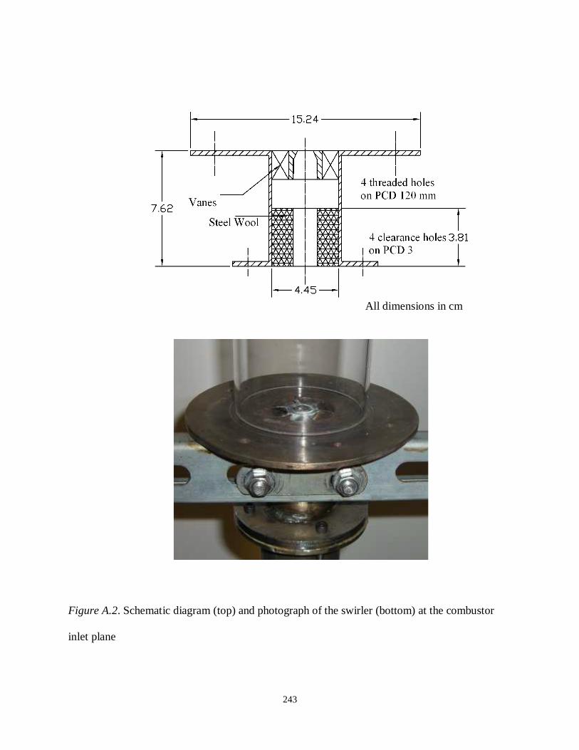
243
Figure A.2. Schematic diagram (top) and photograph of the swirler (bottom) at the combustor
inlet plane
All dimensions in cm

244
Figure A.3. Injector details

245
Figure A.4. Effect of atomizing air on flame images
-4 -2 0 2 4-4 -2 0 2 4-4 -2 0 2 40
5
10
15
20
25
-4 -2 0 2 40
5
10
15
20
25
-4 -2 0 2 4 -4 -2 0 2 4
-4 -2 0 2 4-4 -2 0 2 4-4 -2 0 2 40
5
10
15
20
25
b. Biodiesel
a. Diesel
c. Biooil
15% AA 20% AA 25% AA

246
Figure A.5. Axial profiles of emissions for diesel, (a) NOx, (b) CO
Axial Distance (cm)
CO
conc
entr
atio
n(p
pm)
0
0
10
10
20
20
30
30
40
40
50
50
0 0
50 50
100 100
150 150
200 200
250 250
300 300
350 350
400 400
15% AA20% AA25% AA
(b)
Axial Distance (cm)
NO
xco
nce
ntr
atio
n(p
pm)
0
0
10
10
20
20
30
30
40
40
50
50
0 0
20 20
40 40
60 60
80 80
15% AA20% AA25% AA
(a)
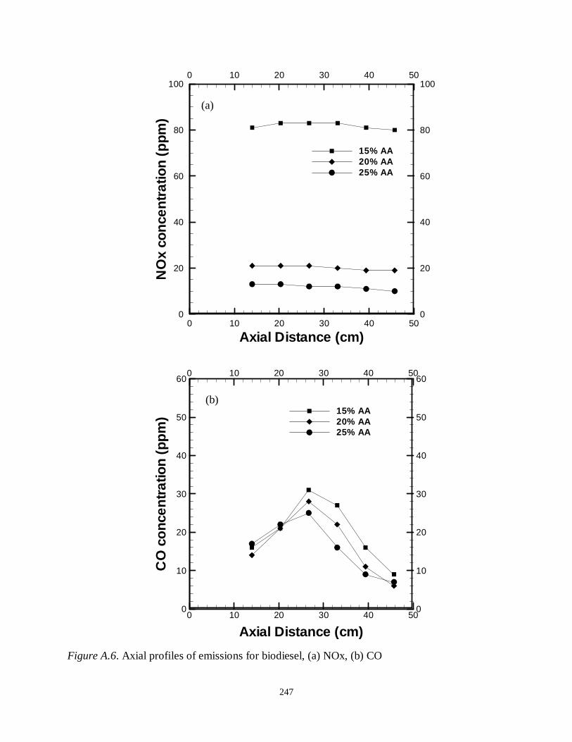
247
Figure A.6. Axial profiles of emissions for biodiesel, (a) NOx, (b) CO
Axial Distance (cm)
CO
conc
entr
atio
n(p
pm
)
0
0
10
10
20
20
30
30
40
40
50
50
0 0
10 10
20 20
30 30
40 40
50 50
60 60
15% AA20% AA25% AA
(b)
Axial Distance (cm)
NO
xco
nce
ntr
atio
n(p
pm)
0
0
10
10
20
20
30
30
40
40
50
50
0 0
20 20
40 40
60 60
80 80
100 100
15% AA20% AA25% AA
(a)

248
Figure A.7. Axial profiles of emissions for biooil, (a) NOx, (b) CO
Axial Distance (cm)
NO
xco
nce
ntr
atio
n(p
pm)
0
0
10
10
20
20
30
30
40
40
50
50
0 0
40 40
80 80
120 120
160 160
200 200
15% AA20% AA25% AA
(a)
Axial Distance (cm)
CO
conc
entr
atio
n(p
pm)
0
0
10
10
20
20
30
30
40
40
50
50
0 0
30 30
60 60
90 90
120 120
150 150
15% AA20% AA25% AA
(b)

249
Figure A.8. Radial profiles of emissions for diesel, (a) NOx, (b) CO
Radial Distance (cm)
NO
xco
ncen
trat
ion
(ppm
)
-4
-4
-2
-2
0
0
2
2
4
4
0 0
20 20
40 40
60 60
80 80
15% AA20% AA25% AA
(a)
Radial Distance (cm)
CO
conc
entr
atio
n(p
pm)
-4
-4
-2
-2
0
0
2
2
4
4
0 0
5 5
10 10
15 15
20 20
25 25
30 30
15% AA20% AA25% AA
(b)

250
Figure A.9. Radial profiles of emissions for biodiesel, (a) NOx, (b) CO
Radial Distance (cm)
CO
conc
entr
atio
n(p
pm)
-4
-4
-2
-2
0
0
2
2
4
4
0 0
30 30
60 60
90 90
120 120
150 150
15% AA20% AA25% AA
(b)
Radial Distance (cm)
NO
xco
ncen
trat
ion
(ppm
)
-4
-4
-2
-2
0
0
2
2
4
4
0 0
20 20
40 40
60 60
80 80
100 100
15% AA20% AA25% AA
(a)

251
Figure A.10. Radial profiles of emissions for biooil, (a) NOx, (b) CO
Radial Distance (cm)
NO
xco
ncen
trat
ion
(ppm
)
-4
-4
-2
-2
0
0
2
2
4
4
0 0
40 40
80 80
120 120
160 160
200 200
15% AA20% AA25% AA
(a)
Radial Distance (cm)
CO
conc
entr
atio
n(p
pm)
-4
-4
-2
-2
0
0
2
2
4
4
0 0
10 10
20 20
30 30
40 40
50 50
15% AA20% AA25% AA
(b)

252
Figure A.11. Axial profiles of emissions for 15% AA, (a) NOx, (b) CO
∗∗∗∗∗
∗
Axial Distance (cm)
NO
xco
ncen
trat
ion
(ppm
)
0
0
10
10
20
20
30
30
40
40
50
50
0 0
30 30
60 60
90 90
120 120
150 150
180 180
DieselBiodieselBiooilSOMESOEE
∗
(a)
∗∗
∗∗∗
∗
Axial Distance (cm)
CO
conc
entr
atio
n(p
pm)
0
0
10
10
20
20
30
30
40
40
50
50
0 0
50 50
100 100
150 150
200 200
250 250
300 300
DieselBiodieselBiooilSOMESOEE
∗
(b)

253
Figure A.12. Axial profiles of emissions for 20% AA, (a) NOx, (b) CO
∗∗∗∗∗∗
Axial Distance (cm)
CO
conc
entr
atio
n(p
pm)
0
0
10
10
20
20
30
30
40
40
50
50
0 0
50 50
100 100
150 150
200 200
250 250
300 300
350 350
400 400
DieselBiodieselBiooilSOMESOEE
∗
(b)
∗∗∗∗∗∗
Axial Distance (cm)
NO
xco
ncen
trat
ion
(ppm
)
0
0
10
10
20
20
30
30
40
40
50
50
0 0
30 30
60 60
90 90
120 120
150 150
180 180
DieselBiodieselBiooilSOMESOEE
∗(a)
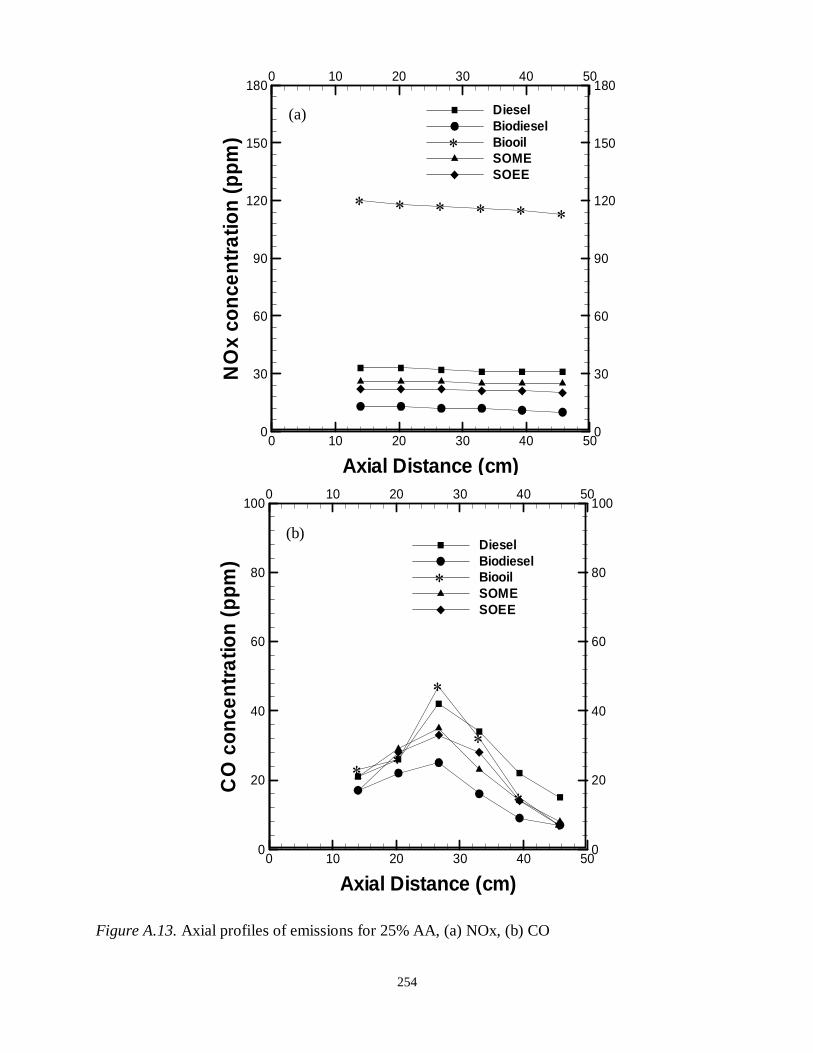
254
Figure A.13. Axial profiles of emissions for 25% AA, (a) NOx, (b) CO
∗∗∗∗∗∗
Axial Distance (cm)
NO
xco
nce
ntr
atio
n(p
pm)
0
0
10
10
20
20
30
30
40
40
50
50
0 0
30 30
60 60
90 90
120 120
150 150
180 180
DieselBiodieselBiooilSOMESOEE
∗(a)
∗∗
∗
∗
∗∗
Axial Distance (cm)
CO
con
cen
trat
ion
(ppm
)
0
0
10
10
20
20
30
30
40
40
50
50
0 0
20 20
40 40
60 60
80 80
100 100
DieselBiodieselBiooilSOMESOEE
∗
(b)
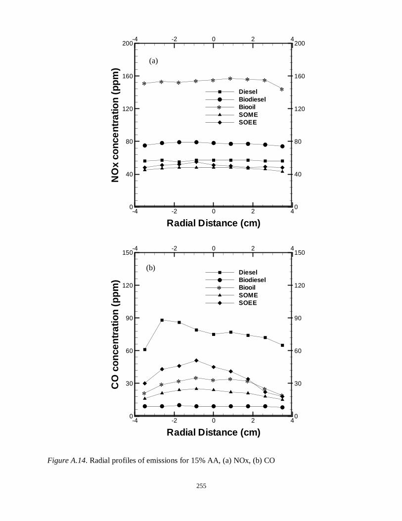
255
Figure A.14. Radial profiles of emissions for 15% AA, (a) NOx, (b) CO
∗∗∗∗∗∗∗∗∗
Radial Distance (cm)
NO
xco
ncen
trat
ion
(pp
m)
-4
-4
-2
-2
0
0
2
2
4
4
0 0
40 40
80 80
120 120
160 160
200 200
DieselBiodieselBiooilSOMESOEE
∗
(a)
∗∗
∗∗∗∗∗∗∗
Radial Distance (cm)
CO
con
cen
trat
ion
(pp
m)
-4
-4
-2
-2
0
0
2
2
4
4
0 0
30 30
60 60
90 90
120 120
150 150
DieselBiodieselBiooilSOMESOEE
∗
(b)

256
Figure A.15. Radial profiles of emissions for 20% AA, (a) NOx, (b) CO
∗∗∗∗∗∗∗∗∗
Radial Distance (cm)
NO
xco
nce
ntr
atio
n(p
pm)
-4
-4
-2
-2
0
0
2
2
4
4
0 0
40 40
80 80
120 120
160 160
200 200
DieselBiodieselBiooilSOMESOEE
∗
(a)
∗∗∗∗∗∗∗∗∗
Radial Distance (cm)
CO
con
cen
trat
ion
(ppm
)
-4
-4
-2
-2
0
0
2
2
4
4
0 0
20 20
40 40
60 60
80 80
DieselBiodieselBiooilSOMESOEE
∗
(b)
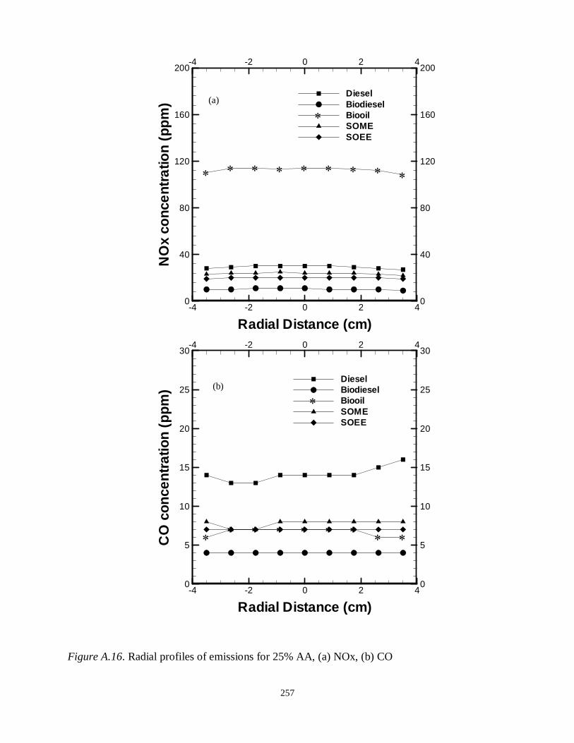
257
Figure A.16. Radial profiles of emissions for 25% AA, (a) NOx, (b) CO
∗∗∗∗∗∗∗∗∗
Radial Distance (cm)
CO
con
cen
trat
ion
(pp
m)
-4
-4
-2
-2
0
0
2
2
4
4
0 0
5 5
10 10
15 15
20 20
25 25
30 30
DieselBiodieselBiooilSOMESOEE
∗(b)
∗∗∗∗∗∗∗∗∗
Radial Distance (cm)
NO
xco
ncen
trat
ion
(pp
m)
-4
-4
-2
-2
0
0
2
2
4
4
0 0
40 40
80 80
120 120
160 160
200 200
DieselBiodieselBiooilSOMESOEE
∗(a)
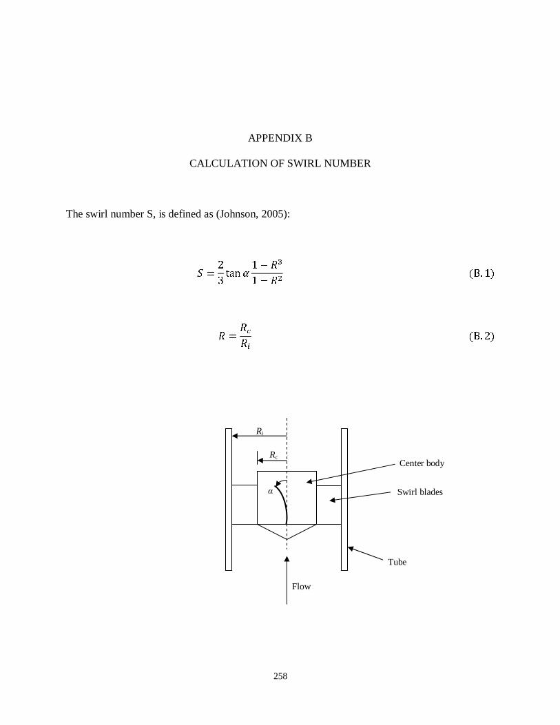
258
APPENDIX B
CALCULATION OF SWIRL NUMBER
The swirl number S, is defined as (Johnson, 2005):
� = 23 tan � 1− ��1− �� (B.1) � = ���� (B.2)
Rc
Ri
Swirl blades
Center body
Tube
α
Flow

259
Thus, for swirler in Chapter 3,
Ri = 2.0 cm
Rc = 1.0 cm
α = 62°
S = 1.5
And for swirler in Chapter 5,
Ri = 1.3 cm
Rc = 0.7 cm
α = 48.9°
S = 0.9

260
APPENDIX C
CALCULATION OF AIR FLOW RATE IN LFE
To determine the air flow rate using the LFE, differential pressure, absolute pressure and
temperature must be measured, as specified by the manufacturer. The equation is of the form:
� = �� ∗ ∆� + � ∗ ∆�� ∗ ���� (C. 1) Where:
Q = actual volumetric flow rate, CFM
B, C = flow coefficients derived from calibration
∆P = differential pressure, inH2O
µstd = viscosity of flowing gas at 20 °C, micropoise
µf = viscosity of flowing gas at flowing temperature, micropoise
The actual volumetric flow rate in liters per minute, LPM, is given by: �� = � ∗ 28.317 (C. 2) (1ft3 = 28.317 L)
Calibration coefficients are presented in Table C.1 for LFE used for air flow rate measurements
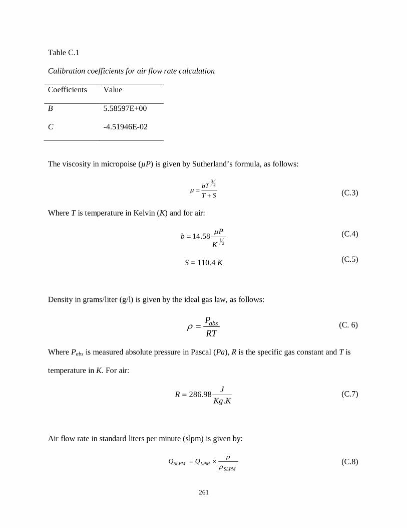
261
Table C.1
Calibration coefficients for air flow rate calculation
Coefficients Value
B 5.58597E+00
C -4.51946E-02
The viscosity in micropoise (µP) is given by Sutherland’s formula, as follows:
ST
bT
+=
23
µ
Where T is temperature in Kelvin (K) and for air:
21
58.14K
Pb
µ=
S = 110.4 K
Density in grams/liter (g/l) is given by the ideal gas law, as follows:
RT
Pabs=ρ
Where Pabs is measured absolute pressure in Pascal (Pa), R is the specific gas constant and T is
temperature in K. For air:
KKg
JR
.98.286=
Air flow rate in standard liters per minute (slpm) is given by:
SLPMLPMSLPM QQ
ρρ
×=
(C.3)
(C.4)
(C.5)
(C. 6)
(C.7)
(C.8)
262
QLPM = volumetric flow rate, LPM
=ρ air density, g/l
Where SLPMρ represents density of air at Standard Temperature and Pressure (STP). STP is
defined as 0 ºC and 1 atm. For air:
SLPMρ =1.276 g/l
Equivalence ratio (Ф) for 100% CH4 combustion is calculated as follows:
AF
AFst=φ
Where AFst is the mass-based stoichiometric Air-Fuel rate. For combustion of CH4 with air:
AFst = 17.11
AF is the actual mass-based Air-Fuel ratio and is given by:
( )( )
44 CH
air
CH
air
Q
Q
m
mAF
⋅
⋅==
ρρ
&
&
(C.9)
(C.10)

263
APPENDIX D
SAMPLE CALCULATIONS OF O2 AND CO2 CONCENTRATIONS
Oxygen (O2) and carbon dioxide (CO2) concentrations are determined from the
equilibrium reaction of each test condition. This result is used to cross-check the equivalence
ratio obtained from the measured fuel and air fuel flow rates. In this section, a sample calculation
of O2 and CO2 concentrations is presented. The procedure is to mass-balance the equilibrium
chemical equation of the case in question, assuming complete combustion, (or no dissociation),
thus, no CO, NOx or other minor species are considered in products containing only CO2, H2O,
N2 and O2. After balancing the equation, the concentration of O2 or CO2 is equal to the number
of moles of O2 or CO2 divided by the total number of moles in the dry product gas. The moles of
H2O must be subtracted from the total moles in the product gas because the sample is dried prior
to entering the gas analyzers. Next, a sample calculation is shown.
The CH4 – air stoichiometric reaction is represented by:
222224 52.72)76.3(2 NCOOHNOCH ++→++
Thus, for a given equivalence ratio Ф < 1, the lean chemical reaction is represented by:
(D.1)

264
2222224 2252.7
2)76.3(2
ONCOOHNOCH
−+++→++
φφφ
For example, for Ф = 0.8, the equation representing the chemical reaction is given by:
2222224 28.0
2
8.0
52.72)76.3(
8.0
2ONCOOHNOCH
−+++→++
Accordingly, the concentrations of O2 and CO2 in the products are given by:
222
22%
nOnNnCO
nOO
++=
222
22%
nOnNnCO
nCOCO
++=
where n is the number of moles of each species.
Substituting:
%6.41002
8.0
2
8.0
52.71
28.0
2
% 2 =×
−++
−=O
%2.91002
8.0
2
8.0
52.71
1% 2 =×
−++=CO
(D.2)
(D.3)
(D.4)
(D.5)
(D.6)
(D.7)

265
The O2 and CO2 concentrations were calculated using measured air and fuel flow rates
for each test case. These calculated values were compared with the O2 and CO2 concentrations
measured experimentally by the gas analyzer at the center of the combustor. Table D.1 shows a
summary of the results.
Table D.1
Summary of O2 and CO2 calculated and experimental results
Q (slpm) Ф
Calculated
Based on air and fuel
flow rates
Experimental
Measured by gas
analyzer
%O2 %CO2 %O2 %CO2
1020 0.65 7.9 7.3 7.0 8.0
0.75 5.7 8.6 4.6 9.5
1400 0.65 7.9 7.3 7.3 7.8
0.75 5.7 8.6 5.0 9.2
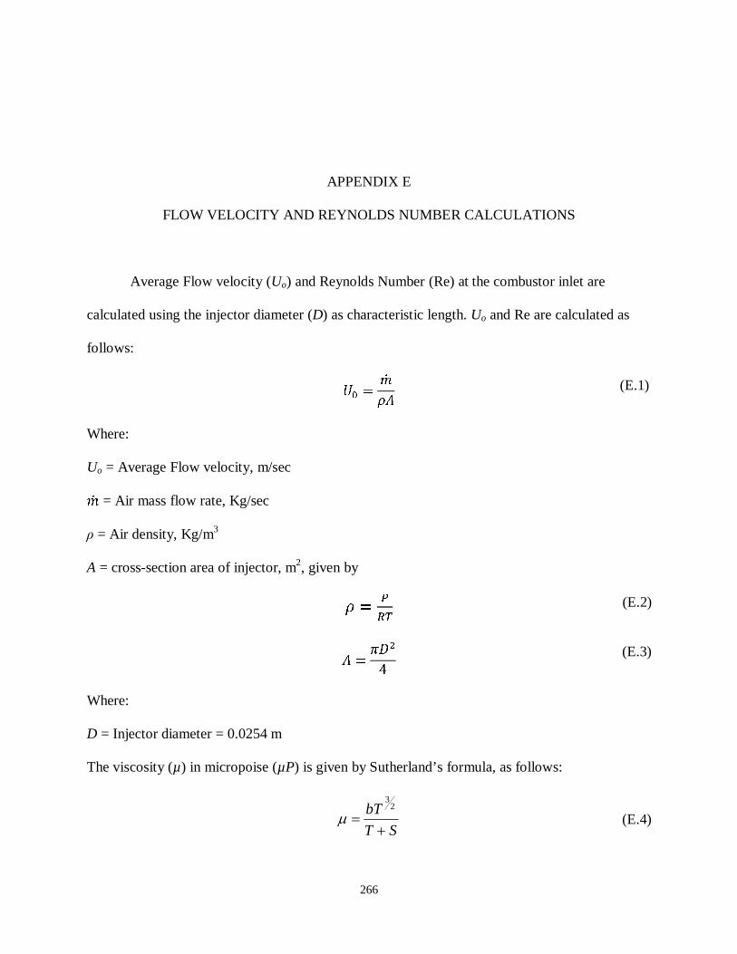
266
APPENDIX E
FLOW VELOCITY AND REYNOLDS NUMBER CALCULATIONS
Average Flow velocity (Uo) and Reynolds Number (Re) at the combustor inlet are
calculated using the injector diameter (D) as characteristic length. Uo and Re are calculated as
follows: �� = ����
Where:
Uo = Average Flow velocity, m/sec �� = Air mass flow rate, Kg/sec
ρ = Air density, Kg/m3
A = cross-section area of injector, m2, given by � = ��� � = ���4
Where:
D = Injector diameter = 0.0254 m
The viscosity (µ) in micropoise (µP) is given by Sutherland’s formula, as follows:
ST
bT
+=
23
µ
(E.2)
(E.1)
(E.3)
(E.4)

267
Where T is temperature in Kelvin (K) and for air:
21
58.14K
Pb
µ=
S = 110.4 K
µρ DU o=Re
For test conditions of this study, Uo and Re results are summarized in Table E.1.
Table E.1
Summary of flow velocity and Reynolds number calculations �� (Kg/min)
Q (slpm)
Tinlet (°C)
Pinlet (psi)
ρ (Kg/m3) µ (Pa.s) Uo (m/s) Re
1.3 1020
20 14.8 1.21 1.81x10⁻⁵ 35.3 50876
130 15.9 0.95 2.30 x10⁻⁵ 45.1 31353
260 17.0 0.77 2.79 x10⁻⁵ 55.8 18588
1.8 1400
20 15.3 1.25 1.81 x10⁻⁵ 47.2 62998
130 16.4 0.98 2.30 x10⁻⁵ 60.6 36248
260 17.2 0.77 2.79 x10⁻⁵ 76.4 22638
2.6 2040
20 34.2 2.81 1.81 x10⁻⁵ 30.4 116613
130 36.2 2.16 2.30 x10⁻⁵ 39.6 60635
260 36.2 1.63 2.79 x10⁻⁵ 52.4 42026
(E.5)
(E.6)
(E.7)

268
APPENDIX F
SOUND PRESSURE LEVEL CALCULATION SCRIPT
This Matlab script is used to calculate total sound pressure level (dB) and A-scale (dBA)
the one-third octave sound pressure signal. An FFT of the time domain pressure signal is done in
LabVIEW. Then the total SPL is calculated using the script presented next. The total SPL is
based on a reference pressure of 20 µPa.
%Determine power per one-third octave frequency band
j=1;
for i=91:113
band1(i)=Prms(i); %generating array
end
P(j)=sum(band1); %total power in frequency band and generating SPL array
j=j+1;
for i=113:141
band2(i)=Prms(i); %generating array
end
P(j)=sum(band2); %total power in frequency band
j=j+1;
for i=141:178

269
band3(i)=Prms(i); %generating array
end
P(j)=sum(band3); %total power in frequency band and generating SPL array
j=j+1;
for i=178:226
band4(i)=Prms(i); %generating array
end
P(j)=sum(band4); %total power in frequency band and generating SPL array
j=j+1;
for i=226:281
band5(i)=Prms(i); %generating array
end
P(j)=sum(band5); %total power in frequency band and generating SPL array
j=j+1;
for i=281:356
band6(i)=Prms(i); %generating array
end
P(j)=sum(band6); %total power in frequency band and generating SPL array
j=j+1;
for i=356:451
band7(i)=Prms(i); %generating array
end
P(j)=sum(band7); %total power in frequency band and generating SPL array

270
j=j+1;
for i=451:561
band8(i)=Prms(i); %generating array
end
P(j)=sum(band8); %total power in frequency band and generating SPL array
j=j+1;
for i=561:701
band9(i)=Prms(i); %generating array
end
P(j)=sum(band9); %total power in frequency band and generating SPL array
j=j+1;
for i=701:901
band10(i)=Prms(i); %generating array
end
P(j)=sum(band10); %total power in frequency band and generating SPL array
j=j+1;
for i=901:1121
band11(i)=Prms(i); %generating array
end
P(j)=sum(band11); %total power in frequency band and generating SPL array
j=j+1;
for i=1121:1401
band12(i)=Prms(i); %generating array

271
end
P(j)=sum(band12); %total power in frequency band and generating SPL array
j=j+1;
for i=1401:1776
band13(i)=Prms(i); %generating array
end
P(j)=sum(band13); %total power in frequency band and generating SPL array
j=j+1;
for i=1776:2251
band14(i)=Prms(i); %generating array
end
P(j)=sum(band14); %total power in frequency band and generating SPL array
j=j+1;
for i=2251:2801
band15(i)=Prms(i); %generating array
end
P(j)=sum(band15); %total power in frequency band and generating SPL array
j=j+1;
for i=2801:3551
band16(i)=Prms(i); %generating array
end
P(j)=sum(band16); %total power in frequency band and generating SPL array
j=j+1;

272
for i=3551:4501
band17(i)=Prms(i); %generating array
end
P(j)=sum(band17); %total power in frequency band and generating SPL array
j=j+1;
for i=4501:5616
band18(i)=Prms(i); %generating array
end
P(j)=sum(band18); %total power in frequency band and generating SPL array
j=j+1;
for i=5616:7066
band19(i)=Prms(i); %generating array
end
P(j)=sum(band19); %total power in frequency band and generating SPL array
j=j+1;
for i=7066:8896
band20(i)=Prms(i); %generating array
end
P(j)=sum(band20); %total power in frequency band and generating SPL array
%CALCULATION OF SOUND PRESSURE LEVEL PER ONE-THIRD OCTAVE BAND
Freq_band=[20 25 31.5 40 50 63 80 100 125 160 200 250 315 400 500 630 800 1000 1250
1600]; %Centers of frequency bands

273
SPL=10*log10(P/(4E-10)); %SPL per 1/3 octave band
%CALCULATION OF SOUND PRESSURE LEVEL PER FREQUENCY
Freq=0:0.2:1999.8; %Frequency range, by frequency resolution
dB_per_freq=10*log10(Prms/4E-10); %SPL at each frequency
%CALCULATION OF TOTAL dB
Rel_power=10.^(SPL./10); %Converting dB to relative power to sum dB levels
Sum_Rel_power=sum(Rel_power);
Total_dB=10*log10(Sum_Rel_power);
%CALCULATION OF dBA AND TOTAL dBA
%A-weighting correction factors:
A_factor=[50.50 44.70 39.40 34.60 30.20 26.20 22.50 19.10 16.10 13.40 10.90 8.60 6.60 4.80
3.20 1.90 0.80 0.0 -0.60 -1.00];
SPL_dBA=SPL-A_factor; %Sound pressure level in dBA
Rel_power_dBA=10.^(SPL_dBA./10); %Converting dB to relative power to sum dB levels
Sum_Rel_power_dBA=sum(Rel_power_dBA);
Total_dBA=10*log10(Sum_Rel_power_dBA);

274
APPENDIX G
UNCERTAINTY ANALYSIS
The uncertainty analysis calculation detailed in this section is consistent with the
procedure outlined by Coleman and Steele (1999). The systematic and random errors are
considered for each measured variable and the total uncertainty is given by both errors
propagated in the experimental result. The general data reduction equation is given by:
...),( 3,21 XXXrr = (G.1)
where r is the experimental result determined by Xi measured variables with 95% confidence.
The overall uncertainty of the result Ur is based on the systematic error Br and respective,
random error Pr of the result.
222rrr PBU += (G.2)
The expressions for Br and Pr are given by the systematic and random uncertainty of the
variables Xi, respectively, assuming no correlated precision uncertainties.
∑
∂∂
= 2
2
2
iXi
r BX
rB (G.3)

275
∑
∂∂
= 2
2
2
iXi
r PX
rP (G.4)
The systematic or bias uncertainty BXi is given by each instrument calibration error. The
random uncertainty or precision limit PXi is given by multiple readings of variable Xi and is
calculated as:
N
tStSP X
XX i== (G.5)
where t is the tabulated distribution with 95 % confidence for N-1 degrees of freedom, N is the
number of measurements (readings) and SX is the standard deviation of the sample set. The
standard deviation of the sample population is defined by:
2/12)(
1
1
−−
= ∑ XXN
S ix (G.6)
where the mean of the sample of the N readings is:
∑= iXN
X1
(G.7)
Overall uncertainty Ur is calculated for measured air and fuel flow rates with LFE,
followed by propagated uncertainty in equivalence ratio for experiments presented in Chapter 3.
Next, overall uncertainty is calculated for air and fuel flow measurements, and propagated

276
uncertainty in equivalence ratio for experiments in Chapter 5. Next, overall uncertainties for jet
noise and combustion noise SPL are calculated.
G.1 Flow Measurements, Low Pressure Facility
The uncertainty analysis in this section pertains to flow measurements of air and fuel
presented in Chapter 3. The uncertainty analysis is performed for an air flow rate of 150 slpm
and a fuel flow rate of 10.9 slpm. From Equation G.2, the total uncertainties in air and fuel flow
measurements are:
222AAA PBU += (G.8)
222FFF PBU += (G.9)
Both air and fuel flow rates are measured with a LFE. The bias errors for air BA and fuel
BF are given by manufacturer as 0.5 % of the measured values, thus BA = 0.75 slpm and BF =
0.05 slpm. Table G.1 shows the set of data collected to determine the random uncertainty PA in
the air flow rate and PF in the fuel flow rate, along with the mean values and standard deviations
according to equations G.6 and G.7.

277
Table G.1
Readings for air and fuel random uncertainty calculation, low pressure facility
N Air measurement (slpm) Fuel Measurement (slpm)
1 149.86 10.81
2 149.63 10.84
3 149.93 10.81
4 149.68 10.82
5 149.83 10.83
6 149.42 10.83
Mean Value 149.73 10.82
Standard Deviation 0.19 0.01
Replacing t = 2.571 for five degrees of freedom, the air flow rate random uncertainty is
PA = 0.48 slpm and the fuel flow rate random uncertainty is PF = 0.03. Substituting into
Equations G.8 and G.9 gives: UA = 0.89 slpm and UF = 0.06 slpm.
The uncertainties in measurements of air in LFE, and CH4 in LFE are propagated to
obtain the overall uncertainty in equivalence ratio. The general data reduction equation for
combustion of CH4 is:
A
F52.9=φ
From Equations G.2, G. 3 and G.4, the total uncertainty in equivalence ratio is:
( ) ( )22
22
2FA U
FU
AU
∂
∂+
∂
∂=
φφφ (G.12)
Where 0046.052.9
2−=−=
∂∂
A
F
A
φ and 0635.0
52.9==
∂∂
AF
φ
(G.11)

278
The uncertainties in air and CH4 measurements are respectively UA = ±0.89 and UF =
±0.06. Substituting in Equation G.12 allows:
0056.0±=φU
G.2 Flow Measurements, High Pressure Facility
The uncertainty analysis in this section pertains to flow measurements of air with LFE,
and fuel with mass flow controller, presented in Chapter 5. The uncertainty analysis is performed
for an air flow rate of 1020 slpm and a fuel flow rate of 69.6 slpm. The bias error for air BA is
given by manufacturer as 0.72% of measured value, thus BA = 7.3 slpm. Bias error for fuel BF is
given by manufacturer as 0.5 % of measured value plus 0.1% of full scale, BF = 0.8 slpm. Table
G.2 lists values for random uncertainty calculation.
Table G.2
Readings for air and fuel random uncertainty calculation, high pressure facility
N Air measurement (slpm) Fuel Measurement (slpm)
1 1020 69.5
2 1012 69.3
3 1025 69.7
4 1030 69.6
5 1041 69.6
6 1033 69.5
Mean Value 1027 68.8
Standard Deviation 10.2 0.14
Next, similar to calculations above, it follows that PA = 10.7 slpm, PF = 0.14 slpm. Thus,
UA = ±12.9 and UF = ±0.8, which allows:

279
UØ = ±0.01.
G.3 Pressure Measurements
The uncertainty analysis in this section pertains to pressure measurements across
injector/combustor presented in Chapter 5. The uncertainty analysis is performed for a pressure
of 101.3 KPa. The bias error BP is given by manufacturer as 0.2% of measured value, thus BP =
0.2 KPa. Table G.3 lists values for random uncertainty calculation.
Table G.3
Readings for pressure random uncertainty calculation, high pressure facility
N Air measurement (slpm)
1 100.6
2 100.6
3 101.3
4 102.0
5 101.3
6 101.3
Mean Value 101.2
Standard Deviation 0.53
Similar to calculations above, it follows that PP = 0.6 KPa. Thus,
UP = ±0.2 KPa