Department of Quantitative Social Science

Reducing bias due to missing values of theresponse variable by joint modeling withan auxiliary variable

Alfonso MirandaSophia Rabe-HeskethJohn W. McDonald

DoQSS Working Paper No. 12-05June 2012

DISCLAIMER

Any opinions expressed here are those of the author(s) and notthose of the Institute of Education. Research published in thisseries may include views on policy, but the institute itself takes noinstitutional policy positions.

DoQSS Workings Papers often represent preliminary work andare circulated to encourage discussion. Citation of such a papershould account for its provisional character. A revised version maybe available directly from the author.

Department of Quantitative Social Science. Institute ofEducation, University of London. 20 Bedford way, LondonWC1H 0AL, UK.

Reducing bias due to missing values of the re-sponse variable by joint modeling with an aux-iliary variableAlfonso Miranda∗, Sophia Rabe-Hesketh†, John W. McDonald‡§

Abstract. In this paper, we consider the problem of missing values of a con-tinuous response variable that cannot be assumed to be missing at random.The example considered here is an analysis of pupil’s subjective engagementat school using longitudinal survey data, where the engagement score fromwave 3 of the survey is missing due to a combination of attrition and itemnon-response. If less engaged students are more likely to drop out and lesslikely to respond to questions regarding their engagement, then missingnessis not ignorable and can lead to inconsistent estimates. We suggest alleviat-ing this problem by modelling the response variable jointly with an auxiliaryvariable that is correlated with the response variable and not subject to non-response. Such auxiliary variables can be found in administrative data, in ourexample, the National Pupil Database containing test scores from nationalachievement tests. We estimate a joint model for engagement and achieve-ment to reduce the bias due to missing values of engagement. A Monte Carlostudy is performed to compare our proposed multivariate response approachwith alternative approaches such as the Heckman selection model and inverseprobability of selection weighting.

JEL classification: C13, C33, I21.

Keywords: Auxiliary variable, joint model, multivariate regression, notmissing at random, sample selection bias, seemingly-unrelatedregressions, selection model, SUR.

∗Department of Quantitative Social Science, Institute of Education, University of London.E-mail: A.Miranda@ioe.ac.uk.†Department of Quantitative Social Science, Institute of Education, University of Lon-don; and Graduate School of Education, University of California, Berkeley. E-mail:sophiarh@berkeley.edu.‡Department of Quantitative Social Science, Institute of Education, University of London.E-mail: John.McDonald@ioe.ac.uk.§This research was supported by ESRC grant RES-576-25-0014 by the ESRC NationalCentre for Research Methods ADMIN node at the Institute of Education.

1. Introduction

Olsen (2006) pointed out that “Perhaps the greatest unexploited opportunity for survey

projects lies in administrative data.” In this paper, we analyse an incomplete continuous

survey response when the survey data are linked to complete administrative data. Linkage

between survey and administrative data opens possibilities for new strategies to handle

missing survey data. When missingness cannot be assumed to be ignorable, one strategy

follows the recommendations by Little and Rubin (1999, p. 1130) who stated that

“Given the problems inherent in nonignorable modeling, we have generally

advocated trying to make the ignorability assumption as plausible as possible

by collecting as much information about incomplete cases as possible, and

then including this information for inferences via model-based approaches

such as multiple imputation.”

This strategy is usually interpreted as including the auxiliary information as extra control

or explanatory variables to make a missing at random (MAR) assumption more realis-

tic. Instead, we exploit the linked data by choosing a continuous variable recorded in

the administrative data that is strongly correlated with the continuous survey response.

We propose using this auxiliary administrative variable as an additional response and

modelling it jointly with the survey response. The model is a multivariate regression

or seemingly unrelated regresion (SUR) model in which the error terms of the response

and auxiliary variable are allowed to be correlated. The parameters are estimated by

maximum likelihood, exploiting all the data available.

To the best of our knowledge, our proposed strategy for handling missing survey data

has not been discussed before. This approach is attractive when, besides the survey,

researchers have access to high quality supplementary information such as administrative

data. Administrative data are usually well maintained and often complete, i.e., do not

suffer from item non-response and/or attrition. Our proposed joint modelling strategy

may be used with either cross-sectional or longitudinal surveys with missing data. The

approach is particularly attractive given the recent increasing availability of linked survey

5

and administrative data for scientific research. For example, in the USA the Current

Population Survey and the Survey of Income and Program Participation are linked to

administrative records on social security earnings and benefits generated by the Social

Security Administration.

We use our proposed strategy for handling missing data on pupil’s subjective en-

gagement at school at age 16 in the Longitudinal Survey of Young People in England

(LSYPE), which have been linked to school administrative records from the National

Pupil Database (NPD). Engagement at age 16, which corresponds to the third wave of

the survey, is missing for nearly 30% of the sample due to a combination of attrition and

item non-response. We expect youngsters to be more likely to drop out and less likely

to answer questions regarding their engagement at school when they feel less engaged.

As a consequence, there are potential problems of sample selection bias if only available

sample data are analysed. We use NPD data on achievement, measured by test scores, as

auxiliary information. Achievement is correlated with engagement and is never missing

because it comes from the NPD. We investigate the role of income, English language

and ethnicity on pupil’s subjective engagement at school at age 16. We do not want to

control for achievement. Instead we use a joint modeling approach to make the MAR

assumption more plausible.

The paper is organised as follows. Section 2 introduces notation, describes our pro-

posed modelling approach and two alternative methods for handling missing data, namely

the Heckman selection model and inverse probability of selection weighting. It also

presents the main contribution of this paper, which is establishing conditions under which

the proposed approach will reduce sample selection bias compared with ordinary least

squares. In Section 3, we use our method to model pupil’s subjective engagement at

school. Next, Section 4 compares our approach with the two alternatives using a Monte

Carlo study. Finally, a discussion is given in Section 5.

6

2. Proposed seemingly-unrelated regressions (SUR) strategy

2.1. General idea

The main objective is to estimate a linear regression model with response variable yi for

individual i (i = 1, . . . , N) and with K covariates xi (including the constant). Variable yi

is observed only if a selection condition (si = 1) is met and is missing otherwise (si = 0).

The condition for the survey response to be missing at random (MAR) can then be

written as P(si | yi,xi) = P(si | xi).

When MAR is violated, ignoring the missingness process can lead to inconsistent

estimators. In this paper, we suggest making the MAR assumption more plausible by

modelling yi jointly with an auxiliary variable ai, that is correlated with yi given xi and

never (or rarely) missing. The MAR condition then becomes P(si | yi,xi, ai) = P (si |

xi, ai). Let s∗i be a latent continuous variable such that si = 1 if s∗i > 0 and si = 0

otherwise. Under multivariate normality of (yi, s∗i , ai)

′ given xi, the conditions for MAR

with and without auxiliary information become

Cor(yi, s∗i | xi, ai) = 0 (1)

and

Cor(yi, s∗i | xi) = 0, (2)

respectively.

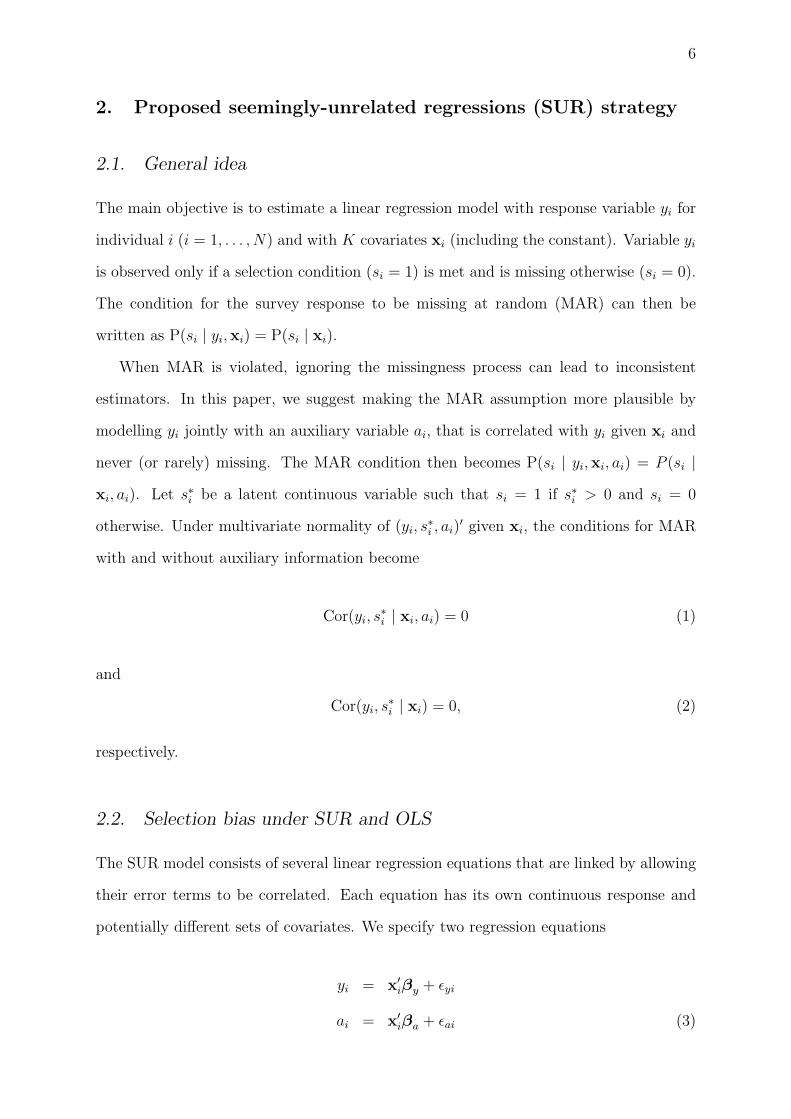
2.2. Selection bias under SUR and OLS

The SUR model consists of several linear regression equations that are linked by allowing

their error terms to be correlated. Each equation has its own continuous response and

potentially different sets of covariates. We specify two regression equations

yi = x′iβy + εyi

ai = x′iβa + εai (3)

7

where βy and βa are regression coefficients and the error terms εyi and εai are assumed

to have a bivariate normal distribution with zero means, standard deviations σy and σa,

and correlation ρ. We let both regression equations contain the same set of covariates.

We now consider different models for the probability that the response variable yi is

observed. A probit model for si can be written as a linear model for the corresponding

latent continuous response s∗i ,

s∗i = x′iβs + θyi + αai + εsi, (4)

where βs, θ, and α are regression coefficients, the error term εsi ∼ N(0, 1) is independent

of the error terms in (3), and the selection indicator takes the value 1 if s∗i > 0 and the

value 0 otherwise.

The model allows selection to depend on the covariates in the model for yi, on the

response variable itself, and on the auxiliary variable ai. When the regression model for

yi is estimated by ordinary least squares (OLS), data are MAR if θ = 0 and α = 0. For

the SUR model, MAR requires only that θ = 0.

A necessary condition for the SUR strategy to deliver (sample selection) bias reduction

compared with OLS is that the auxiliary response ai should carry information about the

missing response yi over and above what is already explained by the covariates. In other

words, we require

Cor(ai, yi | xi) = Cor(εai, εyi | xi) ≡ ρ 6= 0. (C1)

Condition (C1), however, does not guarantee bias reduction. Bias results from violation

of the mean-independence of the error term εyi for yi in the selected sample, E(εyi|xi, si =

1) 6= 0. It can be shown that this expectation, referred to here as ‘bias’, for OLS and

SUR is given by

biasOLS(θ, α, ρ) =

[θσ2

y + αρσyσa√θ2σ2

y + α2σ2a + 2θαρσyσa + 1

]λOLS

i (θ, α, ρ) (5)

biasSUR(θ, α, ρ) =

θσ2

y(1− ρ2)√θ2σ2

y(1− ρ2) + 1

λSUR

i (θ, α, ρ) (6)

8

with

λOLSi (θ, α, ρ) = λi

(x′iβ

∗s√

θ2σ2y + α2σ2

a + 2θαρσyσa + 1

)(7)

λSURi (θ, α, ρ) = λi

x′iβ

∗s√

θ2σ2y(1− ρ2) + 1

(8)

where β∗s = (βs +θβy +αβa) and λ(·) = φ(·)/Φ(·) represents the inverse Mill’s ratio with

φ(·) and Φ(·) denoting the standard normal density and cumulative density functions,

respectively.

As expected, the bias for the two approaches is zero when the respective MAR con-

ditions hold, i.e., biasOLS(θ = 0, α = 0, ρ) = 0 and biasSUR(θ = 0, α, ρ) = 0. Also note

that when θ 6= 0 and α = 0, the bias of OLS is not a function of ρ, whereas the bias of

SUR is a function of ρ that attains a maximum when ρ = 0, with biasSUR(θ, α = 0, ρ =

0) = biasOLS(θ, α = 0, ρ = 0). In other words, biasSUR(θ, α = 0, ρ) ≤ biasOLS(θ, α = 0, ρ).

If the data are not MAR for either approach, i.e., θ 6= 0, a sufficient (but not necessary)

condition for SUR to be less biased than OLS (which we will refer to as bias reduction)

is therefore that α = 0. This implies,

P (si | xi, yi, ai) = P (si | xi, yi). (C2)

The condition is that selection does not depend on ai once yi and xi are conditioned on.

In the setting of equation (4), this holds if α = 0. Notice that (C2) is an untestable

assumption because, by definition, yi is missing when si = 0.

According to Wooldridge (2002b, p. 64) (C1) and (C2) together make ai an imperfect

proxy for yi in the selection equation si. A proxy satisfies the additional requirement that

E(yi | ai,xi) = E(yi | ai). Figure 1 (a) shows a path diagram for the SUR model when

conditions (C1) and (C2) are met and ai is an imperfect proxy for yi, whereas Figure 1 (b)

shows the case where ai is a proxy for yi. In these diagrams, squares represent observed

variables and circles unobserved variables (yi is in a circle because it is sometimes missing),

long arrows represent regressions (linear or probit) and short arrows represent error terms

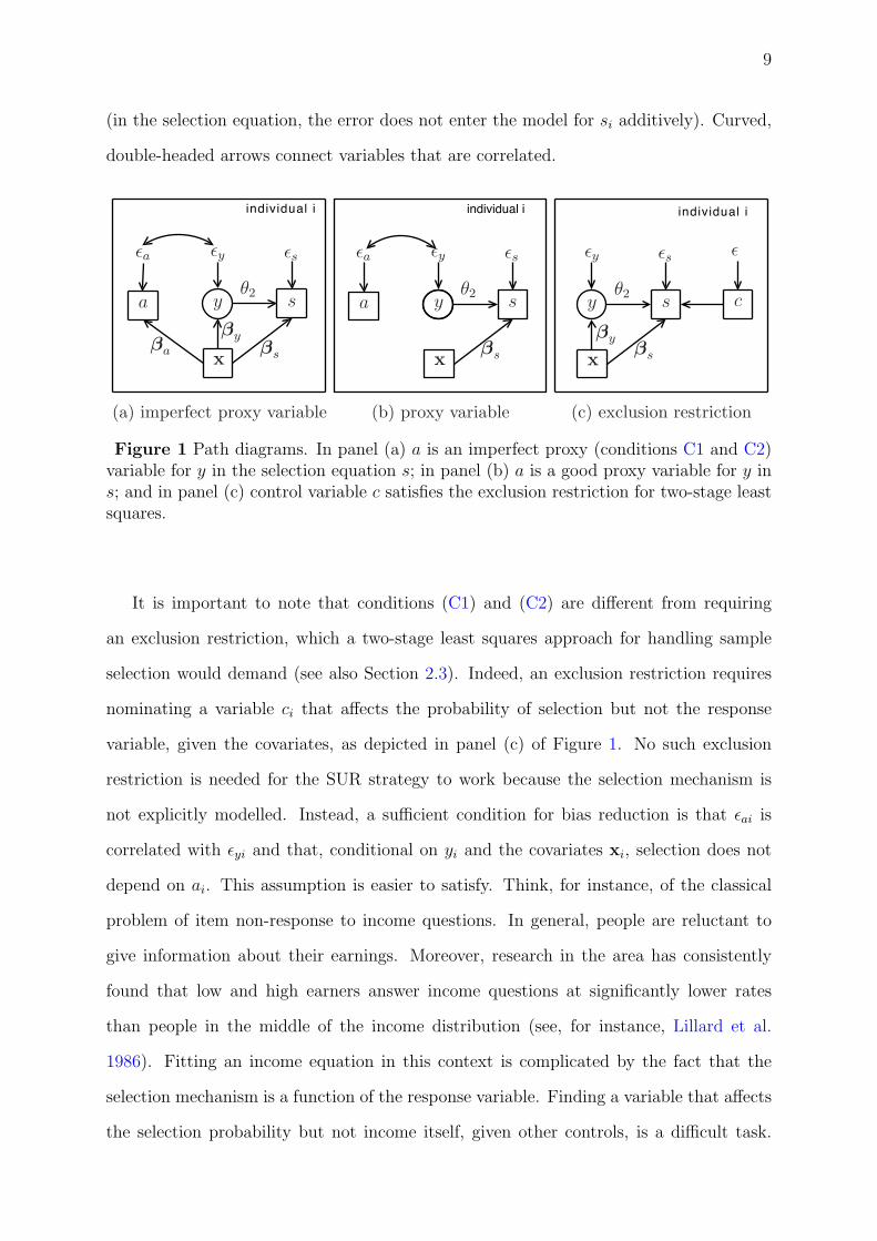
9

(in the selection equation, the error does not enter the model for si additively). Curved,

double-headed arrows connect variables that are correlated.

individual i

y sa!2

"a "y "s

x!a

!y!s

(a) imperfect proxy variable

individual i

y sa!2

"a "y "s

x!s

(b) proxy variable

individual i

y s!2

"y "s

x

!y!s

#c

"c

(c) exclusion restriction

Figure 1 DAG diagram — Main response is denoted by y and selection dummy by S.The potentially missing ordinal covariate is denoted by xi. Circles represent unobserved,or latent, variables whereas rectangles represent observed variables. Arrows connectinglatent and/or observed variables represent linear and non-linear relationships. Vectors r,w and z represent control variables. Coe!cients are written alongside the relevant arrow.Subfigure (a) depicts the model when the ordinal covariate xi is missing, while subfigure(b) depicts the model when the ordinal covariate xi is observed.

Missing ordinal covariates with informative

selection

Alfonso Miranda!, Sophia Rabe-Hesketh†

Abstract. This paper considers the problem of parameter estimation in a model fora continuous response variable Y when an important ordinal explanatory variable X ismissing for a large proportion of the sample and the selection rule (non-deletion fromthe sample) S is function of unobservables after conditioning on all observed controls —i.e. there is selection in unobservables. We suggest addressing this endogenous selectionproblem by joint modeling of the selection mechanism, the ordinal explanatory variableX, and the response variable Y . The method is illustrated by re-examining the problemof ethnic gaps in educational achievement at age 16 in England.

JEL classification: C13, C35, I21.

Keywords: Missing covariate, sample selection, latent class models, ordinal variables,NMAR.

!Corresponding author. Department of Quantitative Social Science, Institute of Education, Universityof London. 20 Bedford Way, London WC1H 0AL, UK. E-mail: A.Miranda@ioe.ac.uk

†Graduate School of Education and Graduate Group in Biostatistics, University of California, Berkeley,USA. Institute of Education, University of London, London, UK. E-mail: sophiarh@berkeley.edu

Figure 1 Path diagrams. In panel (a) a is an imperfect proxy (conditions C1 and C2)variable for y in the selection equation s; in panel (b) a is a good proxy variable for y ins; and in panel (c) control variable c satisfies the exclusion restriction for two-stage leastsquares.

It is important to note that conditions (C1) and (C2) are different from requiring

an exclusion restriction, which a two-stage least squares approach for handling sample

selection would demand (see also Section 2.3). Indeed, an exclusion restriction requires

nominating a variable ci that affects the probability of selection but not the response

variable, given the covariates, as depicted in panel (c) of Figure 1. No such exclusion

restriction is needed for the SUR strategy to work because the selection mechanism is

not explicitly modelled. Instead, a sufficient condition for bias reduction is that εai is

correlated with εyi and that, conditional on yi and the covariates xi, selection does not

depend on ai. This assumption is easier to satisfy. Think, for instance, of the classical

problem of item non-response to income questions. In general, people are reluctant to

give information about their earnings. Moreover, research in the area has consistently

found that low and high earners answer income questions at significantly lower rates

than people in the middle of the income distribution (see, for instance, Lillard et al.

1986). Fitting an income equation in this context is complicated by the fact that the

selection mechanism is a function of the response variable. Finding a variable that affects

the selection probability but not income itself, given other controls, is a difficult task.

10

It is easier, however, to think of an additional response variable that is: (1) correlated

with income, (2) unlikely to suffer from item non-response, (3) does not belong to the

main equation, and (4) is unlikely to affect selection given income. Say, expenditure on

clothing. Hence, this will be a good candidate for an auxiliary variable for implementing

the SUR strategy. Notice this auxiliary variable does not comply with the requirements

for imposing a valid exclusion restriction because: (1) it is an endogenous variable in the

s∗i equation (because it is correlated with the response and yi is not observed), and (2) it

does not belong in the s∗i equation.

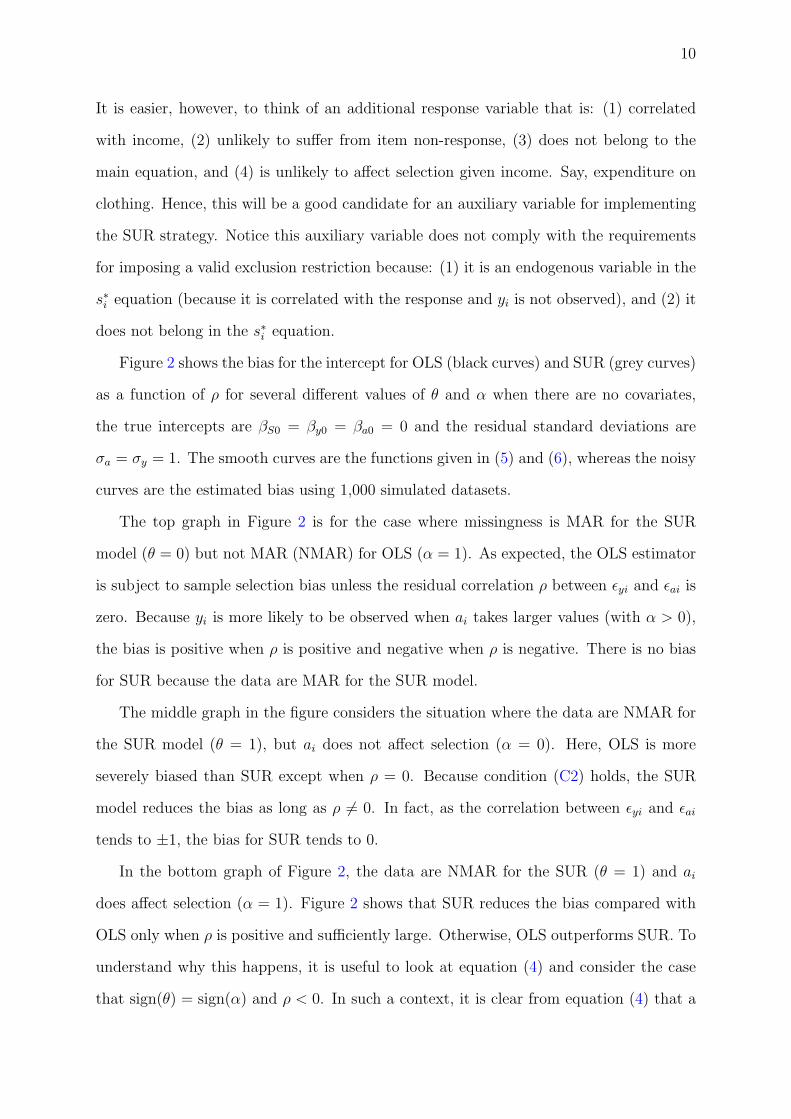
Figure 2 shows the bias for the intercept for OLS (black curves) and SUR (grey curves)

as a function of ρ for several different values of θ and α when there are no covariates,

the true intercepts are βS0 = βy0 = βa0 = 0 and the residual standard deviations are

σa = σy = 1. The smooth curves are the functions given in (5) and (6), whereas the noisy

curves are the estimated bias using 1,000 simulated datasets.

The top graph in Figure 2 is for the case where missingness is MAR for the SUR

model (θ = 0) but not MAR (NMAR) for OLS (α = 1). As expected, the OLS estimator

is subject to sample selection bias unless the residual correlation ρ between εyi and εai is

zero. Because yi is more likely to be observed when ai takes larger values (with α > 0),

the bias is positive when ρ is positive and negative when ρ is negative. There is no bias

for SUR because the data are MAR for the SUR model.

The middle graph in the figure considers the situation where the data are NMAR for

the SUR model (θ = 1), but ai does not affect selection (α = 0). Here, OLS is more

severely biased than SUR except when ρ = 0. Because condition (C2) holds, the SUR

model reduces the bias as long as ρ 6= 0. In fact, as the correlation between εyi and εai

tends to ±1, the bias for SUR tends to 0.

In the bottom graph of Figure 2, the data are NMAR for the SUR (θ = 1) and ai

does affect selection (α = 1). Figure 2 shows that SUR reduces the bias compared with

OLS only when ρ is positive and sufficiently large. Otherwise, OLS outperforms SUR. To

understand why this happens, it is useful to look at equation (4) and consider the case

that sign(θ) = sign(α) and ρ < 0. In such a context, it is clear from equation (4) that a

11

MAR (θ = 0;α = 1)

-.8

-.6

-.4

-.2

0.2

.4.6

.8

-1 -.5 0 .5 1

!

OLS with S=1 SUR

NMAR (θ = 1;α = 0)

-.8

-.6

-.4

-.2

0.2

.4.6

.8

-1 -.5 0 .5 1

!

OLS with S=1 SUR

NMAR (θ = 1;α = 1)

-.8

-.6

-.4

-.2

0.2

.4.6

.8

-1 -.5 0 .5 1

!

OLS with S=1 SUR

Figure 2 Sample selection bias. Black curves represent OLS bias, grey curves representSUR bias. Smooth curves represent the theoretical bias and noisy curves represent biasestimates using simulations.

12

positive (negative) increment of yi will be partially compensated by a negative (positive)

increment of ai because the two variables are negatively correlated and θ and α have the

same sign. This cancelling out makes the MAR assumption more valid. The performance

of OLS improves as more of the effect of yi on si is wiped out.1 Now, because the SUR

model has the effect of stripping out the effect of εai from yi and si, the partial effect of

yi on si cannot be counteracted by the partial effect of ai on si. For these reasons, given

the right conditions, OLS can outperform SUR when α 6= 0.

2.3. Alternative methods for handling missing data

We consider two alternative approaches for handling missing data when auxiliary in-

formation ai is available: inverse probability of selection weighting and the Heckman

selection model. Inverse probability of selection weighting involves fitting the probit

selection model in (4), with θ = 0, to the whole sample to obtain predicted selection

probabilities given covariates and auxiliary information pi = P (Si | xi, ai). Then, in a

second stage, the equation for yi in (9) is estimated for the selected sample (with si = 1)

by weighted least squares (WLS) with weights given by 1/pi. This will deliver consistent

estimators for βy (Horvitz and Thompson 1952)(Little and Robin 1987, p. 57) (Robins

and Rotnitzky 1995, p. 123) (Wooldridge 2002a, p. 122). However, because information

has been discarded in the second stage, WLS estimators are inefficient. Small pi and

hence large weights can lead to large standard errors (Basu 1971).

The Heckman selection model (Heckman 1979) is a joint model for yi and s∗i . If θ 6= 0

and α 6= 0, the data are not missing at random, i.e. selection is informative. In the

equations for yi and s∗i ,

yi = x′iβy + εyi (9)

s∗i = x′iβ∗s + ξsi (10)

1A similar argument shows that if sign(θ) 6= sign(α) and ρ > 0 the OLS estimator will benefit fromthe cancelling out of the effect of yi on si.

13

the errors εyi and ξsi are correlated because

ξsi = θεyi + αεai + εsi. (11)

Because of the correlation between the error terms, equations (9) and (10) should be

fitted as a system in order to obtain a consistent estimator of βy. One straightforward

option will be estimating the parameters by maximum likelihood (ML).

Notice that when fitting the Heckman model one cannot condition selection on ai

because this variable is correlated with yi and, as a consequence, is correlated with the

composite error (θyi + εsi) in the model for s∗i . In other words, ai is endogenous in the

selection equation and including it as part of the control variables will cause the probit

estimator for βs to be inconsistent.

The ML estimator is based on a joint normality assumption for the error terms εyi

and ξsi and is efficient. Instead of using ML, it is possible to fit the model by limited

information maximum likelihood (LIML), which is a two-step estimation method. In the

first step, a probit model is fitted on the whole sample (because si and xi are always

observed) to obtain an estimate for the parameters in the selection equation β∗s. In the

second step, a least squares estimator is used to fit

yi = x′iβy + δλi + ui (12)

using the selected (si = 1) sample. This regression includes the inverse Mill’s ratio,

λi =φ(x′iβs)

Φ(x′iβs),

as an additional explanatory variable, or ‘control function’. Here, δλi is a correction term

that ensures E(ui | xi, λi) = 0. As a consequence, once this term is plugged-in, the OLS

estimator for βy is consistent. LIML has the advantage of removing the assumption of

joint normality for εyi and ξsi. It is enough to suppose that ξsi is normally distributed,

and no restrictive distributional assumptions for εyi are needed (Wooldridge 2002b, p.

14

562) (Vella 1998). Hence, LIML delivers a consistent estimator for βy under weaker

conditions than ML. In exchange for the weaker conditions, LIML has the disadvantage

of delivering an estimator that is no longer efficient (Vella 1998, Puhani 2000).

Because of the non-linearity of the inverse Mills ratio function, the Heckman model

is identified by functional form even if the same set of explanatory variables enter both

equations. However, if x′iβ∗s does not vary sufficiently, λi will be well-approximated by a

linear function. This can cause severe multicollinearity in (9) and large standard errors for

the parameters of interest βy (Wooldridge 2002b, p. 564). As a consequence, the model is

likely to give rather unrobust results (Vella 1998, p. 135) (Little 1985, p. 1470) (Puhani

2000, p. 57).2 In particular, and more substantially, the researcher cannot be confident

that evidence for bias, i.e. δ 6= 0, is caused by true sample selection bias rather than

model misspecification (Little 1985, p. 1470) (Wooldridge 2002b, p. 564). Specifying at

least one exclusion restriction is therefore the ideal approach. This is equivalent to finding

an instrument ci for si in the yi equation, as is graphically depicted in panel (c) of Figure

1. Obviously, finding a valid candidate for imposing the needed exclusion restriction is

difficult in most cases.

Even if a valid instrument is available, the ML estimator of (9) and (10) will be very

sensitive to misspecification of the distribution of εyi (Little 1985, p. 1473) (Vella 1998, p.

135). Moreover, even though it is more robust, the LIML can also be affected by serious

departures from joint normality because the model still assumes that E(εyi | εsi) is linear

in εsi (see, for instance, Wooldridge 2002b, p. 562). If this condition does not hold,

LIML will not be consistent. To address this problem, various approaches that relax the

linearity of E(εyi | εsi) have been suggested. One approach is the semi-parametric two-

step selection model discussed by Vella (1998). In the first step, a semi-nonparametric

model is fitted using the methods of Gallant and Nychka (1987) to obtain a consistent

estimator of the linear index x′iβ∗s in the binary variable model. Then, as suggested by

Newey (2009), the second step fits an OLS regression for yi in the selected sample, adding

powers of x′iβ∗s to control for selection. This is a control function approach.

2Vella (1998) (p. 135) says that in such a case “. . . the degree of identification is “weak” . . . ”

15

3. Application: missing data on pupil’s subjective engagement

at school

Here we investigate the role of income, English as a second language and ethnicity on

pupil’s subjective engagement at school at age 16. We use the Longitudinal Survey of

Young People in England (LSYPE) linked to the National Pupil Database (NPD). The

pupils were aged 16 in the third wave of the LSYPE. A major challenge is that engagement

at age 16 is missing for nearly 30% of the sample, due to a combination of dropout and

item non-response.

We expect pupils to be more likely to continue participating in the survey and to

answer questions regarding their engagement at school when they feel more engaged (or

unlikely to respond if they are extremely disengaged). Therefore θ may be positive,

leading to sample selection bias. To address the issue, we use achievement scores from

administrative data as auxiliary variables. Achievement and engagement are expected to

be positively correlated (ρ > 0). After controlling for engagement, achievement may not

substantially affect the probability of selection, but if it does, we expect the effect to be

positive (α > 0), so that it is likely that SUR will lead to a bias reduction compared with

OLS. We will use achievement scores at ages 14 and 16, denoted a1i and a2i, as auxiliary

variables. As another auxiliary variable zi, we will use engagement at age 14, although

this response was missing for 16.4% of the sample. The SUR model for the application is

yi = x′iβy + εyi

a1i = x′iβa1 + εa1i

a2i = x′iβa2 + εa2i

zi = x′iβz + εzi (13)

Where βy, βa1, βa2 and βz are regression coefficients and the error terms εyi, εa1i, εa2i

and εzi are assumed to have a multivariate normal distribution with zero means and an

unstructured covariance matrix.

16

We use the SUR strategy described in Section 2, but with three auxiliary variables:

achievement a1i and a2i at ages 14 and 16 and engagement zi at age 14. Results are then

compared with those obtained by alternative estimation methods, including OLS, WLS,

the selection model suggested by Heckman (1979), and the semi-parametric two-step

selection model of Vella (1998).

3.1. Longitudinal Survey of Young People in England and National Pupil

Database

We use data from the LSYPE linked to the NPD. The NPD is the set of administrative

records for the whole population of pupils in state maintained schools in England and

contains information on a limited number of key variables. The NPD was used as a

sampling frame for the LSYPE and the two data sets can be linked at the pupil level.

The target population of the LSYPE is year 9 secondary school students, aged between

13 and 14 in 2004, in state maintained, pupil referral units, and independent schools in

England. The LSYPE is a two-stage survey. In the first stage, schools were sampled from

strata of deprived / non deprived schools, with deprived schools being over-sampled by a

factor of 1.5. In the second stage, pupils from minority ethnic groups (Indian, Pakistani,

Bangladeshi, Black African, Black Caribbean, and Mixed) were over-sampled with the

objective to achieve 1,000 issued students in each group. The total issued sample had

21,000 students. The design ensures that within stratum and within ethnic group all

students have the same probability of selection.

We use data from the LSYPE wave 1 (W1) and wave 3 (W3), i.e. students aged 14 nd

16. Students with serious learning disabilities with a full statement of special education

needs (FSEN) are excluded from the analytical sample, but we include pupils with partial

special education needs (SEN). A total of 838 schools were sampled to the LSYPE and 647

schools (73%) participated. School non-response was a problem particularly in London

where only 57% of the selected schools participated. Out of the 21,000 issued interviews,

a total of 15,770 students / households co-operated with the study (74% response rate),

yielding 13,914 (66%) full interviews and 1,856 partial interviews (9%). After excluding

17

1,108 students from private schools and 498 FSEN students we are left with 14,164

observations. This is our analytical sample.

3.2. Variables

Engagement at age 16 is our response variable of interest. Engagement scores, both at

age 14 and 16, are constructed from pupil’s responses to 8 subjective questions in the

LSYPE:

• I am happy when I am at school;

• School is a waste of time;

• School work is worth doing;

• Most of the time I don’t want to go to school;

• On the whole I like being at school;

• I work as hard as I can in school;

• In a lesson, I often count the minutes till it ends;

• The work I do in lessons is a waste of time.

Each question has 4 response categories, from 1 (strongly agree) to 4 (strongly disagree).

Negative questions were code-reversed. Next, we calculated the (raw) sum of the 8 items.

Preliminary inspection showed that the distribution of the raw sum is seriously negatively

0.5

11

.5

0 1 2 3 4 0 1 2 3 4

Wave 1 Wave 3

De

nsity

EngagementGraphs by LSYPE wave

Figure 3. Engagement histogram by LSYPE wave.

18

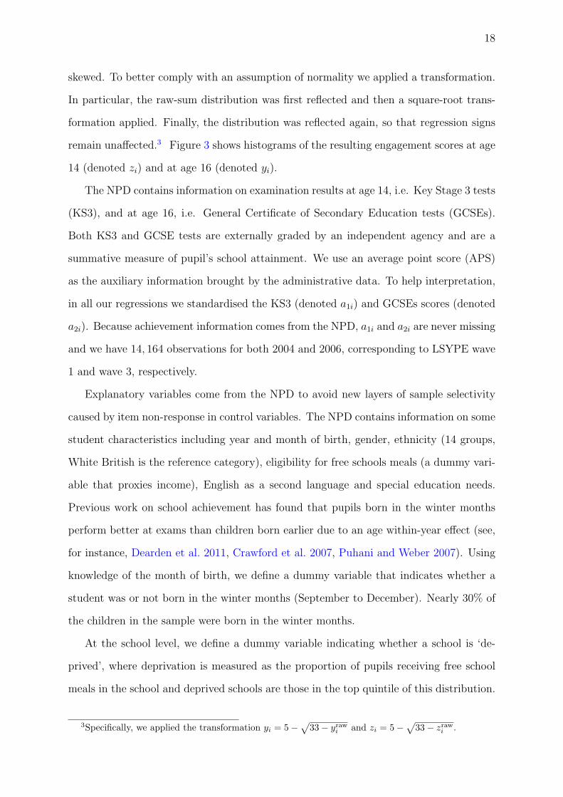
skewed. To better comply with an assumption of normality we applied a transformation.

In particular, the raw-sum distribution was first reflected and then a square-root trans-

formation applied. Finally, the distribution was reflected again, so that regression signs

remain unaffected.3 Figure 3 shows histograms of the resulting engagement scores at age

14 (denoted zi) and at age 16 (denoted yi).

The NPD contains information on examination results at age 14, i.e. Key Stage 3 tests

(KS3), and at age 16, i.e. General Certificate of Secondary Education tests (GCSEs).

Both KS3 and GCSE tests are externally graded by an independent agency and are a

summative measure of pupil’s school attainment. We use an average point score (APS)

as the auxiliary information brought by the administrative data. To help interpretation,

in all our regressions we standardised the KS3 (denoted a1i) and GCSEs scores (denoted

a2i). Because achievement information comes from the NPD, a1i and a2i are never missing

and we have 14, 164 observations for both 2004 and 2006, corresponding to LSYPE wave

1 and wave 3, respectively.

Explanatory variables come from the NPD to avoid new layers of sample selectivity

caused by item non-response in control variables. The NPD contains information on some

student characteristics including year and month of birth, gender, ethnicity (14 groups,

White British is the reference category), eligibility for free schools meals (a dummy vari-

able that proxies income), English as a second language and special education needs.

Previous work on school achievement has found that pupils born in the winter months

perform better at exams than children born earlier due to an age within-year effect (see,

for instance, Dearden et al. 2011, Crawford et al. 2007, Puhani and Weber 2007). Using

knowledge of the month of birth, we define a dummy variable that indicates whether a

student was or not born in the winter months (September to December). Nearly 30% of

the children in the sample were born in the winter months.

At the school level, we define a dummy variable indicating whether a school is ‘de-

prived’, where deprivation is measured as the proportion of pupils receiving free school

meals in the school and deprived schools are those in the top quintile of this distribution.

3Specifically, we applied the transformation yi = 5−√

33− yrawi and zi = 5−

√33− zraw

i .

19

Finally, we know the geographic area where the school is located (9 regions, London is

the reference category). Again, these variables are never missing and, as a consequence,

there are 14, 164 observations for both 2004 and 2006.

The British Market Research Bureau (BMRB) was the main contractor for LSYPE

wave 1. BMRB subcontracted part of the interview work to other two companies, NOP

and IPSOS-MORI. All three companies worked across all geographic areas covered by

the LSYPE and in some cases worked together in the field. We have information, for all

individuals, on which company approached them for interview. Because contractors have

different field experience and incentives to perform, the company that did the interview

is likely to be a predictor of item non-response at wave 1. Further, a bad / poor interview

experience at wave 1 is probably a factor that determines attrition and item non-response

at wave 3. We cannot think why this variable should be associated with a pupil’s school

engagement or attainment after controlling for the covariates and, as a consequence, it is

a good candidate for imposing exclusion restrictions in the Heckman selection model.

3.3. Descriptive results

The response variable yi, engagement at age 16, is missing for 4, 232 (30%) cases, 2, 738

(64.70%) due to survey attrition and 1, 494 (35.3%) due to survey item non-response.

Engagement at age 14, which we use as an auxiliary variable zi, is missing for 2, 021

cases, 15.6% of the sample. Interestingly, the missingness patterns are not monotone.

For some pupils zi is missing, but yi is not missing (1, 261 individuals or 8.9% of the

sample). In total, there are 8, 671 students for whom we observe engagement at both

times.

Table 1 shows the pairwise correlations between engagement and achievement. As

expected, achievement at ages 14 and 16 is highly positively correlated, with a correlation

coefficient of 0.75. Engagement scores at age 14 and 16 are also positively correlated,

though the correlation coefficient is just 0.53. The cross-correlations are all positive as

well, ranging between 0.18 and 0.37. Interestingly, the correlation between achievement

and engagement is higher at age 16 than at age 14 (0.37 versus 0.18). The reason for this

20

may be that the GCSE exams represent higher stakes than the KS3 exams.

Table 1 Pairwise correlation coefficients. Number of observations used in the calculationof each correlation coefficient is written in brackets.

z y a1 a2

z 1 (11,953)y 0.53 (8,671) 1 (9,932)a1 0.18 (11,953) 0.20 (9,932) 1 (14,164)a2 0.27 (11,953) 0.37 (9,932) 0.75 (14,164) 1 (14,164)

Table 2 Mean engagement z in W1 and mean (standardised) achievement a1 and a2

in W1 and W3 by yi missingness condition. Standard deviations written in parentheses,number of observations written in square brackets, and standard errors written in curlybrackets. ‡denotes that the difference in the first two rows is statistically different fromzero at the 1% level using a t-test and allowing for unequal variances in the yi missingand yi not missing sub-samples.

z a1 a2

yi missing 2.23 (0.69)[3,282] -0.18 (1.00)[4,232] -0.24 (1.05)[4,232]yi not missing 2.34 (0.65)[8,671] 0.15 (0.92)[9,932 ] 0.19 (0.87)[9,932 ]Difference -0.11‡ {0.01} -0.33‡ {0.02} -0.43‡ {0.02}N. obs 11,953 14,164 14,164

Table 2 presents summary statistics by missingness status of engagement at age 16,

yi. Not missing yi is associated with better mean achievement at both age 14 and 16

and with a marginally higher mean engagement score at age 14. A t-test at the 1%

level rejects the null hypothesis that the difference in means for zi across the si = 0 (yi

missing) and si = 1 (yi not missing) sub-samples is zero. Similar conclusions are drawn

for the achievement variables, a1i and a2i. Descriptive statistics of all variable used in the

regressions are given in Table 3.

3.4. Results from regressions

Table 4 reports results from a probit regression for the selection indicator si, where yi is

observed only when si = 1. Among other explanatory variables, we control for previous

(age 14) engagement, zi, previous and current achievement, a1i, a2i, and the company

that carried out the LSYPE interview. Previous engagement is significant at the 1%

level. As expected, a child who is highly engaged at age 14 has better odds of being

21

Table 3 Descriptive statistics. Reference category for categorical variables is indicatedin brackets

Variable Obs Mean Std.Dev. Min Max

Student characteristicsz 11953 2.31 0.67 0.0 4.0y 9932 2.22 0.70 0.0 4.0a1 14164 0.05 0.96 -4.0 1.7a2 14164 0.06 0.95 -2.8 2.0s 14164 0.70 0.5 0 1female 14164 0.50 0.5 0 1Special Educational Needs 14164 0.11 0.3 0 1Winter born 14164 0.32 0.5 0 1Mover year 10 14164 0.02 0.1 0 1English Additional Language 14164 0.22 0.4 0 1Free School Meals 14164 0.17 0.4 0 1White British (reference) 14164 0.62 0.5 0 1White other 14164 0.02 0.1 0 1Mixed 14164 0.06 0.2 0 1Indian 14164 0.07 0.2 0 1Pakistani 14164 0.07 0.3 0 1Bangladeshi 14164 0.05 0.2 0 1Other Asian 14164 0.01 0.1 0 1Black Caribbean 14164 0.04 0.2 0 1Black African 14164 0.04 0.2 0 1Black other 14164 0.00 0.1 0 1Chinese 14164 0.00 0.0 0 1Other 14164 0.01 0.1 0 1Refused 14164 0.01 0.1 0 1No data 14164 0.01 0.1 0 1

School and geographic characteristicsDeprived school 12800 0.09 0.3 0 1London (reference) 14164 0.18 0.4 0 1East Midlands 14164 0.09 0.3 0 1East of England 14164 0.10 0.3 0 1North East 14164 0.05 0.2 0 1North West 14164 0.14 0.3 0 1South East 14164 0.13 0.3 0 1South West 14164 0.08 0.3 0 1West Midlands 14164 0.12 0.3 0 1York 14164 0.11 0.3 0 1

Company which did the LSYPE interviewBMRB 14164 0.44 0.5 0 1NOP 14164 0.44 0.5 0 1MORI 14164 0.11 0.3 0 1Other 14164 0.01 0.1 0 1

highly engaged at age 16 and, at the same time, she is less likely to drop out of the

LSYPE or not to answer the school engagement questions. Achievement at age 16 is also

22

a good predictor of the probability of selection. Interestingly, conditional on achievement

at age 16, selection does not appear to depend upon achievement at age 14. We find also

that children who move schools in year 10, i.e. a year before taking GCSEs, are less likely

to be observed. This is intuitive as moving schools may indicate a major disruption for

the child as well as the family, leading to an increased likelihood of dropout and item

non-response. Among all ethnic groups, only pupils from Black Caribbean and Black

African background are significantly less likely to be observed at the 1% level. Students

who were interviewed by IPSOS-MORI are more likely to be selected into the sample at

a 5% level of significance. All other LSYPE-company dummy variables are statistically

insignificant. Importantly, a Wald test for the exclusion of all the LSYPE-company

dummy variables gives χ2(3) = 6.5 (p-value = 0.09). So, these dummy variables are only

marginally significant in the probit model.

Because, by definition, we do not observe yi when si = 0, it is impossible to know

whether selection depends on engagement at age 16 after controlling for engagement at

age 14 and achievement at ages 14 and 16. Hence, there is no way of testing for a MAR

versus NMAR missing data mechanism (or non-informative versus informative selection).

We can, for instance, suppose that the data are NMAR and fit a Heckman sample

selection model. Table 5 reports results from such regressions. We do not condition on

zi, a1i and a2i because these variables are endogenous in the model for s∗i and including

them will cause the Heckman model to deliver an inconsistent estimator. The LSYPE-

company dummy variables are excluded from the yi equation and, therefore, are used

to identify the model beyond functional form. A Wald test for the exclusion of these

dummy variables in the selection equation gives χ2(3) = 9.7 (p-value = 0.02). This

suggests that the exclusion restriction may be valid, though the chi-square is relatively

low. Keeping these qualifying facts in mind, we conclude from Table 5 that the Heckman

selection model gives evidence that there are important sample selection problems caused

by attrition and item non-response in these data, with Cor(εyi, ξsi) estimated as 0.685.

Table 5 also reports estimates from the semi-parametric two-step regression suggested by

23

Table 4 Probit estimates for probability of non-missing en-gagement variable in LSYPE W3. ‡(†) Significant at 1% (5%).Engagement in W1 is denoted z, achievement in W1 is denoteda1, and achievement in W3 is denoted a2.

Coeff. SE

Student characteristicsz 0.078‡ 0.008a1 -0.035 0.021a2 0.291‡ 0.021Female 0.001 0.025Special Educational Needs 0.083 0.043Winter born -0.004 0.027Mover year 10 -0.304‡ 0.095English Additional Language -0.088 0.059Free SchoolMeals -0.044 0.036White other 0.052 0.110Mixed -0.071 0.056Indian 0.005 0.071Pakistani -0.131 0.074Bangladeshi 0.084 0.083Other Asian -0.052 0.166Black Caribbean -0.236‡ 0.066Black African -0.302‡ 0.074Black other -0.325 0.203Chinese -0.524† 0.238Other -0.252 0.154Refused -0.192 0.138No data -0.023 0.116

School and Geographic characteristicsDeprived school -0.014 0.038Geographic dummy variables Yes

Company which did the LSYPE interviewNOP 0.039 0.027MORI 0.099† 0.045Other -0.141 0.179

N 11,953

Vella (1998).4 In line with the Heckman model, the semi-parametric estimator suggests

that there is some degree of sample selectivity.

Table 6 reports regression results for OLS regression, WLS regression and SUR. The

WLS strategy makes the assumption that the data are MAR once zi, a1i and a2i have been

4Preliminary regressions were fitted using quadratic, cubic, and square power functions of the indexfunction from the first step and the results indicated that the quartic and cubic terms were insignificant.To save space, we report only the regression with a square power function of the first step index.

24

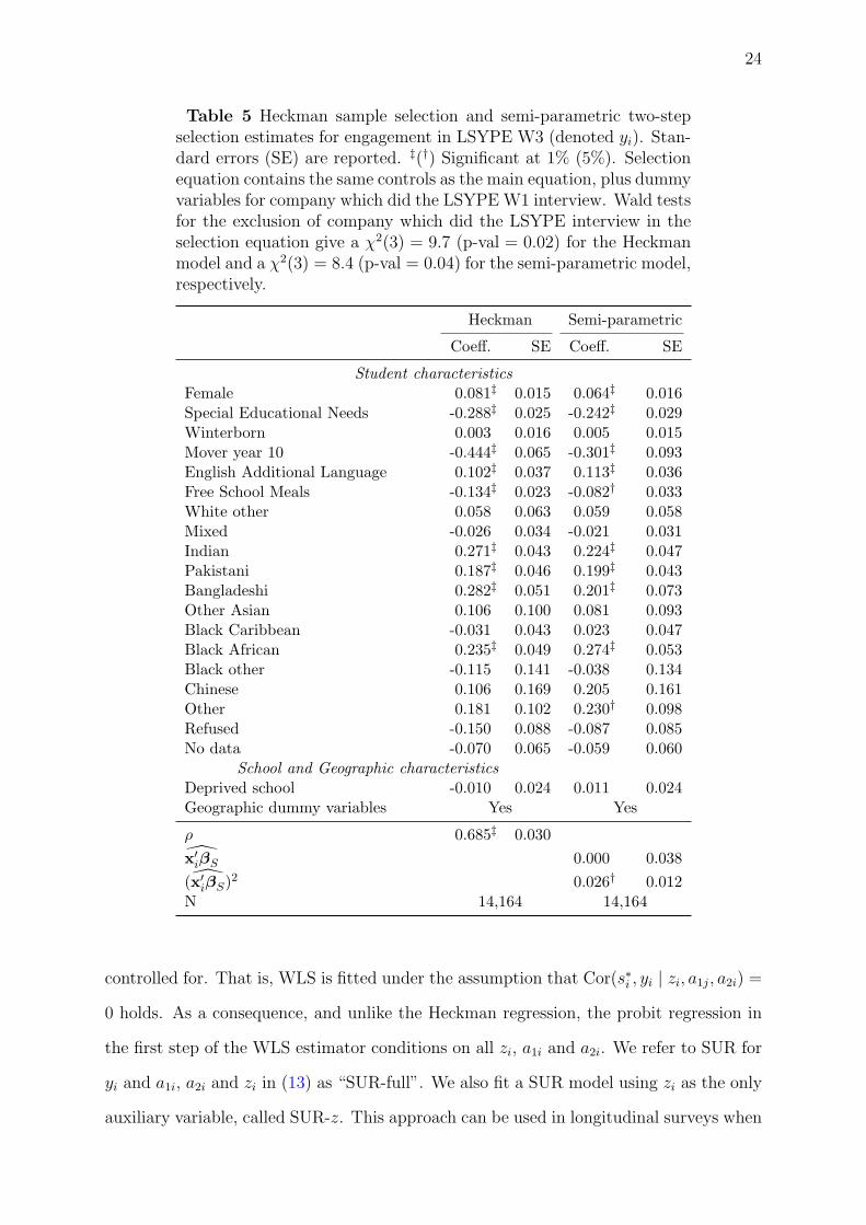
Table 5 Heckman sample selection and semi-parametric two-stepselection estimates for engagement in LSYPE W3 (denoted yi). Stan-dard errors (SE) are reported. ‡(†) Significant at 1% (5%). Selectionequation contains the same controls as the main equation, plus dummyvariables for company which did the LSYPE W1 interview. Wald testsfor the exclusion of company which did the LSYPE interview in theselection equation give a χ2(3) = 9.7 (p-val = 0.02) for the Heckmanmodel and a χ2(3) = 8.4 (p-val = 0.04) for the semi-parametric model,respectively.

Heckman Semi-parametric

Coeff. SE Coeff. SE

Student characteristicsFemale 0.081‡ 0.015 0.064‡ 0.016Special Educational Needs -0.288‡ 0.025 -0.242‡ 0.029Winterborn 0.003 0.016 0.005 0.015Mover year 10 -0.444‡ 0.065 -0.301‡ 0.093English Additional Language 0.102‡ 0.037 0.113‡ 0.036Free School Meals -0.134‡ 0.023 -0.082† 0.033White other 0.058 0.063 0.059 0.058Mixed -0.026 0.034 -0.021 0.031Indian 0.271‡ 0.043 0.224‡ 0.047Pakistani 0.187‡ 0.046 0.199‡ 0.043Bangladeshi 0.282‡ 0.051 0.201‡ 0.073Other Asian 0.106 0.100 0.081 0.093Black Caribbean -0.031 0.043 0.023 0.047Black African 0.235‡ 0.049 0.274‡ 0.053Black other -0.115 0.141 -0.038 0.134Chinese 0.106 0.169 0.205 0.161Other 0.181 0.102 0.230† 0.098Refused -0.150 0.088 -0.087 0.085No data -0.070 0.065 -0.059 0.060

School and Geographic characteristicsDeprived school -0.010 0.024 0.011 0.024Geographic dummy variables Yes Yes

ρ 0.685‡ 0.030x′iβS 0.000 0.038(x′iβS)2 0.026† 0.012N 14,164 14,164

controlled for. That is, WLS is fitted under the assumption that Cor(s∗i , yi | zi, a1j, a2i) =

0 holds. As a consequence, and unlike the Heckman regression, the probit regression in

the first step of the WLS estimator conditions on all zi, a1i and a2i. We refer to SUR for

yi and a1i, a2i and zi in (13) as “SUR-full”. We also fit a SUR model using zi as the only

auxiliary variable, called SUR-z. This approach can be used in longitudinal surveys when

25

administrative data are not available. SUR-z and SUR-full should work well under both

MAR and NMAR if the auxiliary information does not affect the selection mechanism

given yi.

Table 6 Estimates for engagement (y) in LSYPE W3. ‡(†) Significant at 1% (5%).Engagement in W1 is denoted z, achievement in W1 is denoted a1, and achievement inW3 is denoted a2. Control variables from NPD only.

Linear models SUR linear models

OLS WLS SUR-z SUR-full

Coeff. SE Coeff. SE Coeff. SE Coeff. SE

Student characteristicsFemale 0.070‡ 0.014 0.069‡ 0.015 0.072‡ 0.013 0.071‡ 0.013Special Ed. Needs -0.245‡ 0.023 -0.236‡ 0.028 -0.239‡ 0.023 -0.241‡ 0.022Winter born 0.005 0.015 0.002 0.016 0.002 0.014 -0.002 0.014Mover year 10 -0.272‡ 0.061 -0.293‡ 0.076 -0.257‡ 0.058 -0.259‡ 0.057English Add Language 0.114‡ 0.034 0.156‡ 0.038 0.119‡ 0.033 0.124‡ 0.033Free School Meals -0.087‡ 0.021 -0.106‡ 0.024 -0.082‡ 0.020 -0.089‡ 0.020White other 0.059 0.058 0.061 0.064 0.045 0.057 0.040 0.056Mixed -0.021 0.031 -0.009 0.034 -0.020 0.030 -0.018 0.030Indian 0.242‡ 0.039 0.218‡ 0.042 0.254‡ 0.038 0.262‡ 0.038Pakistani 0.196‡ 0.043 0.161‡ 0.047 0.195‡ 0.041 0.206‡ 0.041Bangladeshi 0.238‡ 0.047 0.210‡ 0.053 0.225‡ 0.046 0.246‡ 0.045Other Asian 0.085 0.092 0.047 0.081 0.091 0.090 0.115 0.089Black Caribbean 0.030 0.040 0.039 0.041 0.046 0.038 0.040 0.038Black African 0.294‡ 0.045 0.273‡ 0.050 0.292‡ 0.043 0.317‡ 0.043Black other -0.030 0.132 -0.099 0.212 -0.031 0.126 0.010 0.125Chinese 0.208 0.159 0.141 0.155 0.190 0.151 0.161 0.149Other 0.244† 0.095 0.177 0.119 0.244‡ 0.091 0.249‡ 0.090Refused -0.097 0.082 -0.192† 0.092 -0.068 0.079 -0.078 0.078Nodata -0.063 0.060 -0.054 0.071 -0.052 0.058 -0.062 0.058

School and Geographic characteristicsDeprived school 0.008 0.022 0.005 0.026 0.006 0.021 0.000 0.021Geographic dummies Yes Yes Yes Yes

σz 0.652‡ 0.004 0.652‡ 0.004σy 0.683‡ 0.005 0.691‡ 0.005σa1 0.872‡ 0.005σa2 0.854‡ 0.005ρz,y 0.512‡ 0.008 0.513‡ 0.008ρz,a1 0.189‡ 0.009ρz,a2 0.253‡ 0.009ρy,a1 0.215‡ 0.009ρy,a2 0.385‡ 0.009ρa1,a2 0.714‡ 0.004

N 9,932 8,671 13,214 14,164N×T×J 21,885 50,213

26

Comparing Tables 5 and 6 we draw the following conclusions. The most affected co-

efficients are those for special education needs (SEN), mover year 10, free school meals

(FSM), and Black African. The correction for sample selection suggested by WLS, SUR,

or indeed the semi-parametric two-step selection model for these variables is relatively

small and substantially less than that suggested by the Heckman selection model. Con-

sider, for instance, the mover year 10 variable in Table 6. In this case, WLS suggests a

negative correction of the OLS estimate of around 0.34 times the standard error (se, here-

after), SUR-z gives a positive correction of 0.25se and SUR-full gives a positive correction

of 0.21se. Finally, the semi-parametric two-step selection model suggest a negative cor-

rection of 0.47se. The Heckman selection model suggests a negative correction of 2.82se.

This is probably the most extreme example across all model specifications. The cases of

SEN and FSM are less dramatic. For SEN, WLS suggests a correction of 0.39se whereas

SUR-z and SUR-full suggest 0.26se and 0.17se, respectively. The Heckman selection

model, in contrast, suggests a correction of −1.87se. For FSM and Black African, we

arrive at similar conclusions.

This pattern is repeated across most control variables. Overall, the SUR-full strategy

seems to suggest corrections that are of a similar magnitude as WLS and the semi-

parametric two-step model. Often, the correction is in the same direction.

4. Monte Carlo simulation study

Here we report a Monte Carlo simulation study that investigates how the SUR strategy

performs compared with OLS, WLS, and the Heckman selection model when the missing-

ness process is MAR and NMAR, respectively for the full SUR model. The objective is to

learn whether the full SUR model offers a good alternative to the other methods consid-

ered in terms of bias, root mean squared error, and coverage of confidence intervals. We

also investigate the performance of these estimators under violations of the multivariate

normality assumption.

27

0.1

.2.3

.4Density

-2 0 2 4e1

Figure 4 Marginal (zero centred) gamma distribution obtained from a multivariateFrank copula with parameter 1, gamma margins, unit variances, and correlations equalto 0.5. The parameters of the gamma margins are: shape = 9 and rate = 2.

4.1. Approaches compared

We compare the following estimators: (1) ordinary least squares (OLS); (2) weighted

least squares with known true weights (WLS-true); (3) weighted least squares (WLS);

(4) Heckman sample selection model (Heckman); (5) SUR for zi and yi only (SUR-z); (6)

SUR for zi, yi, a1i and a2i (SUR-full).

4.2. Setup of experiments

Data are simulated from the model specified in (13) under two different assumptions for

the error terms εzi, εyi, εa1i, εa2i: (i) multivariate normal distribution, and (ii) multivariate

non-normal distribution. In both cases the error terms are generated with zero means,

unit variances, and correlations equal to 0.5. To draw from a non-normal multivariate

distribution with the required covariance matrix, we follow Mair et al. (2011) and use a

Frank copula with parameter 1 and gamma margins. We wish to have clear departures

from multivariate normality. As a consequence, the gamma margins are set with shape

parameter 9 and rate parameter 2 so that the distribution is positively skewed and has

a long right tail. Figure 4 gives a histogram of 1, 000 draws from this distribution, with

mean set to 0.

The following aspects of the simulation study remain unchanged regardless of the

28

distribution of the error terms. Replications are indexed with superscript r, with r =

1, . . . , R, where R = 1, 000. In each replication four independent standard normal covari-

ates xri1, . . . , x

ri4 and three independent Bernoulli(0.5) dummy variables dr

i1, . . . , dri3 are

simulated, with i = 1, . . . , N and N = 1, 000. Next, four multivariate error terms εrzi, εryi,

εra1i, εra2i are generated as described in the previous paragraph. Response and auxiliary

variables zri , y

ri , a

r1i, a

r2i are then obtained using equation (13). Finally, the selection vari-

able sri = 1(s∗ri > 0) is generated on the basis of the simulated responses, an independent

standard normal residual εrs, and the following equation:

s∗ri = xr′βs + θ1zri + θ2y

ri + α1a

r1i + α2a

r2i + εrsi. (14)

The selection rule is then used to make yri missing when sr

i = 0.

We vary θ1, θ2, α1 and α2 to change whether the missingness process is MAR for SUR-

full (depending on whether or not θ2 = 0) and to vary the amount of information that

zi, a1i and a2i provide about selection (reflected by the difference between Cov(s∗i , yi | xi)

and Cov(s∗i , yi | xi, zi, a1i, a2i)). With the residual correlations held constant at 0.5, this

depends only on the values of θ1, α1 and α2. Table 7 presents the values of θ1, θ2, α1 and

α2 for each experiment. Whereas experiment 1 and experiment 2 are MAR for SUR-full

(θ2 = 0), experiment 3 to experiment 5 are NMAR for SUR-full and in experiment 3 the

auxiliary variables carry the most information about selection. Table 8 reports the values

of β in each equation and experiment.

Table 7 Parameters θ1, θ2, α1 and α2 for the Monte Carlo simulations. Experiments 1and 2 are MAR for the SUR-full (θ2 = 0), experiments 3 to 5 are NMAR for SUR-fulland in experiment 3 the auxiliary variables carry the most information about selection.

Correlation

Exp. θ1 θ2 α1 α2 (s∗i , yi | xi) (s∗i , yi | xi, zi) (s∗i , yi | xi, zi, a1i, a2i)

1 0.2 0 0.2 0 0.19 0.06 02 0.2 0 0.2 0.2 0.27 0.11 03 0.2 0.2 0 0 0.28 0.17 0.164 0.2 0.2 0.2 0.2 0.42 0.27 0.165 0 0.5 0 0.5 0.57 0.47 0.37

Identical covariates xri are used in all equations. The parameters of substantive in-

29

terest are βy and these are set to 0.34 across all experiments. The regression coefficients

for xri are positive in all equations and are chosen such that the proportion of variance

explained by xri (coefficient of determination) is on average about 0.41 for zr

i and yri and

about 0.38 for the auxiliary variables a1i and a2i. In the selection equation, βs is set so

that the proportion of variance explained by xri , a1i, a2i, z

ri and yr

i is about 0.33 and the

standard deviation of s∗ri is less than or equal to 1.5, on average.5 This ensures that an

extremely large inverse probability of the selection weight occur rarely so that WLS per-

forms reasonably well (more than 95% of the time P(si = 1|xi)−1 ≤ 100 and more than

99% of the time P(si = 1|xi)−1 ≤ 5003.2)). The probability of selection is on average 0.7

across all experiments.

Table 8. Values for βz,βa1,βa2 and βs in each Monte Carlo experiment.

βs

Variable βz βa1βa2

exp 1 exp 2 exp 3 exp 4 exp 5

constant 0.4 0.31 0.25 0.15 0.20 0.15 -0.05 -0.1x1 0.4 0.31 0.25 0.10 0.10 0.10 0.10 0x2 0.4 0.31 0.25 0.20 0.25 0.20 0.20 0x3 0.4 0.31 0.25 0.30 0.30 0.30 0.25 0x4 0.4 0.31 0.25 0.40 0.40 0.40 0.35 0d1 0.1 0.10 0.47 0.10 0.10 0.10 0.10 0d2 0.1 0.31 0.47 0.20 0.20 0.20 0.20 0d3 0.1 0.31 0.47 0.30 0.30 0.30 0.30 0

4.3. Results

Figure 5 presents results for one continuous and one dummy variable, i.e. x1 and d1,

and under the multivariate normality assumption of the error terms. Results for other

variables are similar and not presented.6 We compare estimators in terms of percentage

bias, root mean squared error (RMSE) and coverage of the 95% confidence intervals.

Note that coverage differs significantly from 95% at the 5% level if it is less than 93.6%

or greater than 96.3%.

5Notice that {θ1, θ2, α1, α2} are fixed by the experiment, so β is adjusted to obtain the requiredvariance.

6Additional simulation results are available from the authors upon request.

30

-15

-10

-50

1 2 3 4 5experiment

Percentage bias x1

-25

-20

-15

-10

-50

1 2 3 4 5experiment

Percentage bias d14

56

7

1 2 3 4 5experiment

Mean squared error x1

78

91

011

12

1 2 3 4 5experiment

Mean squared error d1

60

70

80

90

10

0

1 2 3 4 5experiment

Coverage of the 95% confidence interval x1

80

85

90

95

1 2 3 4 5experiment

OLS WLS-TRUE

WLS HECKMAN

SUR-z SUR-full

Coverage of the 95% confidence interval d1

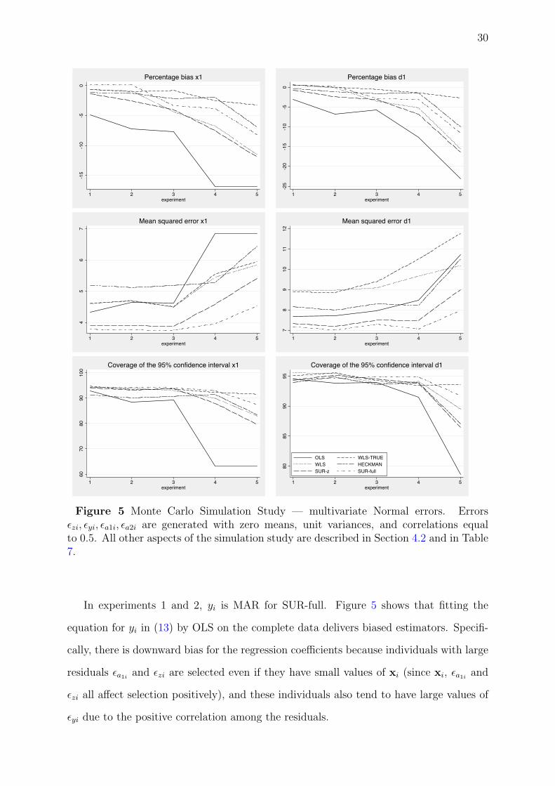
Figure 5 Monte Carlo Simulation Study — multivariate Normal errors. Errorsεzi, εyi, εa1i, εa2i are generated with zero means, unit variances, and correlations equalto 0.5. All other aspects of the simulation study are described in Section 4.2 and in Table7.

In experiments 1 and 2, yi is MAR for SUR-full. Figure 5 shows that fitting the

equation for yi in (13) by OLS on the complete data delivers biased estimators. Specifi-

cally, there is downward bias for the regression coefficients because individuals with large

residuals εa1iand εzi are selected even if they have small values of xi (since xi, εa1i

and

εzi all affect selection positively), and these individuals also tend to have large values of

εyi due to the positive correlation among the residuals.

31

Unsurprisingly, both WLS with known true weights and WLS deliver approximately

unbiased estimators that are well behaved. For the Heckman sample selection model

we obtain some bias that, however small (no more than 3%), is still significant at the

5% level. Coverage for the Heckman model is also below the advertised 95% level in

experiments 1 and 2. SUR-z behaves similarly to the Heckman estimator in terms of

bias, but has smaller RMSE and better coverage. Finally, SUR-full produces the smallest

bias, which is insignificant at the 5% level for all parameters. The RMSE is also the

lowest among all estimators considered and coverage is good for all parameters. These

results are as expected since the missingness process is MAR for SUR-full.

When the data are NMAR for SUR-full in experiments 3 to 5, the picture is less clear-

cut. Certainly, OLS delivers biased estimators with percentage biases between 13% and

23%. The Heckman model gives a less biased estimator, although bias is significant at the

5% level for all parameters and coverage is below 95% for three parameters in experiment

3, two parameters in experiment 4 and all parameters in experiment 5. SUR-full delivers

larger biases than the Heckman estimator and the bias is also significant at the 5% level.

However, the RMSEs are smaller than for the Heckman model. In conclusion, SUR- full

achieves relatively good bias reduction compared with OLS and fares relatively well when

compared to the Heckman sample selection model.

In experiment 3, the data are NMAR for SUR-full and the selection rule does not

depend on the auxiliary information. In this case, our theoretical results suggest that

SUR-full should be less biased than OLS. Figure 5 supports our predictions. Although

the Heckman estimator dominates the SUR-full marginally in terms of bias, SUR-full

gives small biases that fluctuate around 5% which seems acceptable. As before, SUR-full

dominates the Heckman estimator in terms of RMSE and has marginally better coverage.

In experiments 4 and 5, WLS with known true weights also seems to be a good

alternative in terms of bias reduction and coverage. If the true weights are unknown,

however, WLS is clearly dominated by both Heckman model and SUR-full. Finally,

SUR-z achieves some bias reduction compared with OLS, but SUR-full performs much

better.

32

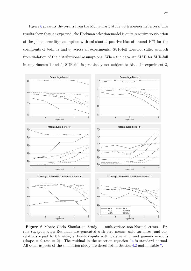
Figure 6 presents the results from the Monte Carlo study with non-normal errors. The

results show that, as expected, the Heckman selection model is quite sensitive to violation

of the joint normality assumption with substantial positive bias of around 10% for the

coefficients of both x1 and d1 across all experiments. SUR-full does not suffer as much

from violation of the distributional assumptions. When the data are MAR for SUR-full

in experiments 1 and 2, SUR-full is practically not subject to bias. In experiment 3,

-20

-10

01

0

1 2 3 4 5experiment

Percentage bias x1

-30

-20

-10

01

0

1 2 3 4 5experiment

Percentage bias d1

.04

.05

.06

.07

.08

1 2 3 4 5experiment

Mean squared error x1

.07

.08

.09

.1.1

1.1

2

1 2 3 4 5experiment

Mean squared error d1

.6.7

.8.9

1

1 2 3 4 5experiment

Coverage of the 95% confidence interval x1

.8.8

5.9

.95

1

1 2 3 4 5experiment

OLS WLSt

WLS Heckman

SUR-z SUR-full

Coverage of the 95% confidence interval d1

Figure 6 Monte Carlo Simulation Study — multivariate non-Normal errors. Er-rors εzi, εyi, εa1i, εa2i Residuals are generated with zero means, unit variances, and cor-relations equal to 0.5 using a Frank copula with parameter 1 and gamma margins(shape = 9, rate = 2). The residual in the selection equation 14 is standard normal.All other aspects of the simulation study are described in Section 4.2 and in Table 7.

33

when the data are NMAR for SUR-full, we still find a moderate bias of −3.53% for the

coefficient of x1 and −2.23% for the coefficient of d1. It is only in the extreme case of

experiment 5 that the SUR-full model has a substantial bias of around 10%. As before,

SUR-full is the least biased estimator with the exception of WLS with known weights.

Even under violations of the multivariate normality assumption, SUR-full dominates all

other estimators as far as the RMSE is concerned and achieves good coverage in all

experiments except experiment 5. In contrast, the Heckman model becomes the worst in

terms of RMSE and has disappointing coverage. As alternatives to SUR-full, SUR-z and

WLS seem to be good options in terms of bias and RMSE.

5. Discussion

The common approaches for dealing with missing data assume that the data are MAR.

The MAR assumption is violated if the selection mechanism depends on the response vari-

able after controlling for the covariates. If the data are NMAR, but complete auxiliary

information from administrative data linked to the survey data are available, new strate-

gies for handling missing survey data are possible. This present paper proposes fitting a

multivariate regression or SUR model for a continuous survey response and continuous

auxiliary responses. For the case of one auxiliary variable, we discussed the conditions

for this approach to achieve bias reduction compared with OLS.

We used our suggested strategy to deal with problems of attrition and item non-

response in the LSYPE, linked to the NPD. In particular, we analysed engagement at age

16 from wave 3 of the LSYPE, using engagement at age 14 from wave 1 of the LSYPE and

test scores for ages 14 and 16 from the NPD as auxiliary variables. The bias corrections

suggested by our SUR strategy and by inverse probability of selection weighting are

relatively small. The SUR bias correction is broadly in line with that suggested by a

semi-parametric two-step sample selection model that is robust to deviations from joint

normality. In contrast, the Heckman selection model suggests a larger bias correction.

We performed Monte Carlo experiments to compare our approach with the Heckman

selection model and with inverse probability of selection weighting. The results sug-

34

gest that SUR performs well compared with the alternatives considered even when the

multivariate normality assumption is violated.

References

Basu, D., 1971. An essay on the logical foundations of survey sampling, part one, in:

Godambe, V., Sprott, D. (Eds.), Foundations of Statistical Inference. Toronto, Holt,

Rinehart and Winston of Canada, pp. 203–242.

Crawford, C., Dearden, L., Meghir, C., 2007. When you are born matters: the impact

of date of birth on child cognitive outcomes in England. Center for the Economics of

Education Discussion paper No. 93.

Dearden, L., Miranda, A., Rabe-Hesketh, S., 2011. Measuring school value added with

administrative data: the problem of missing variables. Fiscal Studies 32, 263–278.

Gallant, A.R., Nychka, D.W., 1987. Semi-nonparametric maximum likelihood estimation.

Econometrica 55, pp. 363–390.

Heckman, J.J., 1979. Sample selection bias as a specification error. Econometrica 47,

153–161.

Horvitz, D.G., Thompson, D.J., 1952. A generalization of sampling without replacement

from a finite universe. Journal of the American Statistical Association 47, pp. 663–685.

Lillard, L., Smith, J., Welch, F., 1986. What do we really know about wages? The

importance of nonreporting and census imputation. Journal of Political Economy 94,

489–506.

Little, R., Robin, D., 1987. Statistical Analysis with Missing Data. Wiley Series in

Probability and Mathematical Statistics, Wiley.

Little, R., Rubin, D., 1999. Adjusting for nonignorable drop-out using semiparametric

nonresponse models: Comment. Journal of the American Statistical Association 94,

1130–1132.

35

Little, R.J.A., 1985. A note about models for selectivity bias. Econometrica 53, 1469–74.

Mair, P., Satorra, A., Bentler, P., 2011. A copula approach to generate non-normal

multivariate data for SEM. Research Report Series / Department of Statistics and

Mathematics, 108. WU Vienna University of Economics and Business, Vienna. http:

//epub.wu.ac.at/3122/.

Newey, W., 2009. Two-step series estimation of sample selection models. Econometrics

Journal 12, S217–S229.

Olsen, R., 2006. Perspectives on longitudinal surveys. Conference on Longitudinal Social

and Health Surveys in an International Perspective, Montreal, January 25-27. http:

//www.ciqss.umontreal.ca/longit/Doc/Randall_Olsen.pdf.

Puhani, P., 2000. The Heckman correction for sample selection and its critique. Journal

of Economic Surveys 14, 53–68.

Puhani, P., Weber, A., 2007. Does the early bird catch the worm? Instrumental variable

estimates of educational effects of age of school entry in Germany. Empirical Economics

32, 359–386.

Robins, J.M., Rotnitzky, A., 1995. Semiparametric efficiency in multivariate regression

models with missing data. Journal of the American Statistical Association 90, 122–129.

Vella, F., 1998. Estimating models with sample selection bias: A survey. The Journal of

Human Resources 33, pp. 127–169.

Wooldridge, J., 2002a. Inverse probability weighted M-estimators for sample selection,

attrition, and stratification. Portuguese Economic Journal 1, 117–139.

Wooldridge, J.M., 2002b. Econometric Analysis of Cross Section and Panel Data. MIT

Press, Cambridge, MA.