Using DIC to compare selection models with non-ignorable missing responses

Abstract

Data with missing responses generated by a non-ignorable missingness mechanism can be anal-ysed by jointly modelling the response and a binary variable indicating whether the response isobserved or missing. Using a selection model factorisation, the resulting joint model consists ofa model of interest and a model of missingness. In the case of non-ignorable missingness, modelchoice is difficult because the assumptions about the missingness model are never verifiable fromthe data at hand. For complete data, the Deviance Information Criterion (DIC) is routinely usedfor Bayesian model comparison. However, when an analysis includes missing data, DIC can beconstructed in different ways and its use and interpretation are not straightforward. In this paper,we present a strategy for comparing selection models by combining information from two measurestaken from different constructions of the DIC. A DIC based on the observed data likelihood is usedto compare joint models with different models of interest but the same model of missingness, and acomparison of models with the same model of interest but different models of missingness is carriedout using the model of missingness part of a conditional DIC. This strategy is intended for usewithin a sensitivity analysis that explores the impact of different assumptions about the two partsof the model, and is illustrated by examples with simulated missingness and an application whichcompares three treatments for depression using data from a clinical trial. We also examine issuesrelating to the calculation of the DIC based on the observed data likelihood.

1 Introduction

Missing data is pervasive in many areas of scientific research, and can lead to biased or inefficient infer-

ence if ignored or handled inappropriately. A variety of approaches have been proposed for analysing

such data, and their appropriateness depends on the type of missing data and the mechanism that

led to the missing values. Here, we are concerned with analysing data with missing responses thought

to be generated by a non-ignorable missingness mechanism. In these circumstances, a recommended

approach is to jointly model the response and a binary variable indicating whether the response is

observed or missing. Several factorisations of the joint model are available, including the selection

model factorisation and the pattern-mixture factorisation, and their pros and cons have been widely

discussed (Kenward and Molenberghs, 1999; Michiels et al., 2002; Fitzmaurice, 2003). In this paper,

attention is restricted to selection models with a Bayesian formulation.

Spiegelhalter et al. (2002) proposed a Deviance Information Criterion, DIC, as a Bayesian measure of

model fit that is penalised for complexity. This can be used to compare models in a similar way to the

Akaike Information Criterion (for non-hierarchical models with vague priors on all parameters, DIC ≈AIC), with the model taking the smallest value of DIC being preferred. However, for complex models,

the likelihood, which underpins DIC, is not uniquely defined, but depends on what is considered as

forming the likelihood and what as forming the prior. With missing data, there is also the question of

what is to be included in the likelihood term, just the observed data or the missing data as well. For

models allowing non-ignorable missing data, we must take account of the missing data mechanism in

addition to dealing with the complication of not observing the full data.

Celeux et al. (2006) (henceforth CRFT) assess different DIC constructions for missing data models, in

the context of mixtures of distributions and random effects models. Daniels and Hogan (2008), Chapter

8, discuss two different constructions for selection models, one based on the observed data likelihood,

DICO, and the other based on the full data likelihood, DICF . However, DICF has proved difficult

1

to implement in practice. The purpose of this paper is to first examine issues of implementation and

usability of DICO and to clarify possible misuse. We then build on this to show how insights from DICO

can be complemented by information from part of an alternative, ‘conditional’, DIC construction, thus

providing the key elements of a strategy for comparing selection models.

In Section 2, we introduce selection models and review the general definition of DIC, before discussing

how DICO and a DIC based on a likelihood that is conditional on the missing data, DICC , can

provide complementary information about the comparative fit of a set of models. Issues concerning

the calculation of DICO are discussed in Section 3, including choice of algorithm, plug-ins and sample

size. In Sections 4 and 5 we describe the use of a combination of DICO and DICC to compare models

for simulated and real data missingness respectively, emphasising that this should be carried out within

the context of a sensitivity analysis rather than to select a single ‘best’ model. We conclude with a

discussion in Section 6.

2 DIC for selection models

We start this section by introducing the selection model factorisation, then discuss the general formula

for DIC, and finally look at different constructions of DIC for selection models.

2.1 Introduction to selection models

Suppose our data consists of a univariate response with missing values, y = (yi), and a vector of fully

observed covariates, x = (x1i, . . . , xpi), for i = 1, . . . , n individuals, and let λ denote the unknown

parameters of our model of interest. y can be partitioned into observed, yobs, and missing, ymis,

values, i.e. y = (yobs,ymis). Now define m = (mi) to be a binary indicator variable such that

mi =

{1: yi observed

0: yi missing

and let θ denote the unknown parameters of the missingness function. The joint distribution of the

full data, (yobs,ymis,m|λ,θ), can be factorised as

f(yobs,ymis,m|λ,θ) = f(m|yobs,ymis,θ)f(yobs,ymis|λ) (1)

suppressing the dependence on the covariates, and assuming that m|y,θ is conditionally independent

of λ, and y|λ is conditionally independent of θ, which is usually reasonable in practice. This factori-

sation of the joint distribution is known as a selection model (Schafer and Graham, 2002). Both parts

of the model involve ymis, so they must be fitted jointly. Consequently assumptions concerning the

model of interest will influence the model of missingness parameters through ymis, and vice versa.

2.2 Introduction to DIC

Deviance is a measure of overall fit of a model, defined as -2 times the log likelihood, D(ϕ) =

−2logL(ϕ|y), with larger values indicating poorer fit. In Bayesian statistics deviance can be sum-

marised in different ways, with the posterior mean of the deviance, D(ϕ) = E{D(ϕ)|y}, suggested as

2

a sensible Bayesian measure of fit (Dempster, 1973) (reprinted as Dempster (1997)), though this is not

penalised for model complexity. Alternatively, the deviance can be calculated using a point estimate

such as the posterior means for ϕ, D(ϕ̄) = D{E(ϕ|y)}. In general we use the notation E(h(ϕ)|y) todenote the expectation of h(ϕ) with respect to the posterior distribution of ϕ|y. However, in more

complex formula, we will occasionally use the alternative notation, Eϕ|y(h(ϕ)).

Spiegelhalter et al. (2002) proposed that the difference between these two measures, pD = D(ϕ)−D(ϕ̄),

is an estimate of the ‘effective number of parameters’ in the model. The DIC proposed by Spiegelhalter

et al. (2002) adds pD to the posterior mean deviance, giving a measure of fit that is penalised for

complexity,

DIC = D(ϕ) + pD. (2)

DIC can also be written as a function of the log likelihood, i.e.

DIC = 2logL{E(ϕ|y)|y} − 4Eϕ|y{logL(ϕ|y)}. (3)

More generally, if D̄ denotes the posterior mean of the deviance and D̂ denotes the deviance calculated

using some point estimate, then DIC = 2D̄ − D̂. We will refer to D̂ as a plug-in deviance, and the

point estimates of the parameters used in its estimation as plug-ins. The value of DIC is dependent

on the choice of plug-in estimator. The posterior mean, which is a common choice, leads to a lack of

invariance to transformations of the parameters (Spiegelhalter et al., 2002), and the reasonableness of

the choice of the posterior mean depends on the approximate normality of the parameter’s posterior

distribution. Alternatives to the posterior mean include the posterior median, which was investigated

at some length by Spiegelhalter et al. (2002), and the posterior mode, which was considered as an

alternative by CRFT.

Further, in hierarchical models we can define the prior and likelihood in different ways depending

on the quantities of interest, which will affect the calculation of both D̄ and D̂ and hence DIC. The

chosen separation of the joint density into prior and likelihood determines what Spiegelhalter et al.

(2002) refer to as the focus of the model.

For complete data, DIC is routinely used by Bayesian statisticians to compare models, a practice

facilitated by its automatic calculation by the WinBUGS software, which allows Bayesian analysis

of complex statistical models using Markov chain Monte Carlo (MCMC) techniques (Spiegelhalter

et al., 2003). WinBUGS calculates DIC, taking D(ϕ) to be the posterior mean of −2logL(ϕ|y), andevaluating D(ϕ̄) as -2 times the log likelihood at the posterior mean of the stochastic nodes. However,

other values of DIC can be obtained by using different plug-ins or a different model focus.

When data include missing values, the possible variations in defining DIC are further increased.

Different treatments of the missing data lead to different specifications, and there is also the question

of what is to be included in the likelihood, just the observed data or the missing data as well.

2.3 DIC based on the observed data likelihood

One construction is based on the observed data likelihood, L(λ,θ|yobs,m),

DICO = 2logL{E(λ,θ|yobs,m)|yobs,m} − 4Eλ,θ|yobs,m{logL(λ,θ|yobs,m)}

3

where

L(λ,θ|yobs,m) ∝∫

f(yobs,ymis,m|λ,θ)dymis.

For a selection model, recalling Equation 1:

L(λ,θ|yobs,m) ∝∫

f(m|yobs,ymis,θ)f(yobs,ymis|λ) dymis

= f(yobs|λ)Eymis|yobs,λ{f(m|yobs,ymis,θ)}.(4)

So the first term in the likelihood is the yobs part of the model of interest, f(yobs|λ), and the second

term evaluates the model of missingness by integrating over ymis. The calculation of the expectation

in Equation 4 creates complexity in the DICO computation.

The fit of the model of interest to yobs is optimised if this part of the model is estimated in isolation,

i.e. we assume ignorable missingness. As soon as we allow for informative missingness by estimating

the model of interest jointly with the model of missingness, the fit of the model of interest part to yobs

necessarily deteriorates. This is because, in a selection model, the same model of interest is applied

to both the observed and the missing data, and so the λ estimates will depend on both yobs and

the imputed ymis. Since the latter are systematically different from the former under an informative

missingness model, the fit of the model of interest to the observed data will necessarily be worse than

if λ had just been estimated using yobs. Consequently, the value of the part of the DICO attributable

to the fit of the model of interest will increase when the model of missingness departs from MAR. This

may partially or completely offset any reduction in the part of DICO attributable to improvements in

fit of the model of missingness (as happens in our simulated example in Section 4.2 and application in

Section 5). Thus, while DICO will indicate which selection model best fits the observed data (yobs and

m), it can be misleading when our true purpose is to compare the fit of selection models to both the

observed and missing data (yobs, m and ymis). Neither DICO nor any other model selection criterion

can answer this question directly as they can never provide information about the fit to the missing

data. However, DICO can provide useful insight into the comparative fit of certain aspects of these

types of models. As we will show, reasonable comparisons can be made using DICO by fixing the

model of missingness part and using it to compare selection models with different models of interest

(conditional on the appropriateness of the missingness model). Even so, we must still be careful how

we use DICO, remembering that it only tells us about the fit of a selection model to the observed data

and nothing about its fit to the missing data.

Because of the fact that the imputed ymis will depend on the model of missingness, and DICO does

not account for the fit to the missing data, we do not recommend using DICO to compare selection

models with different models of missingness. Hence, it would be useful to have an additional model

comparison measure that focusses on the missing data. Clearly we cannot examine the fit of the

missing data as we can for the observed data, but we do have information brought by the missingness

indicator. We would therefore like a DIC construction that allows us to use this additional information

and consider the fit of the model of missingness separately.

4

2.4 Conditional DIC

An alternative option is a conditional DIC, which treats the missing data as additional parameters

(CRFT). This can be written as:

DICC = 2logL{E(λ,θ,ymis|yobs,m)|yobs,m} − 4Eλ,θ,ymis|yobs,m{logL(λ,θ,ymis|yobs,m)}.

For selection models the likelihood on which this is based is

L(λ,θ,ymis|yobs,m) ∝ f(yobs,m|λ,θ,ymis)

= f(yobs|ymis,λ)f(m|yobs,ymis,θ).(5)

For many examples, including all those discussed in this paper, f(yobs|ymis,λ) can be simplified to

f(yobs|λ). In this case DICC only differs from DICO in the second term, f(m|yobs,ymis,θ), which

is evaluated by conditioning on ymis rather than by integrating over it. The plug-ins for DICC

include the missing data, ymis, and are evaluated as E(λ,θ,ymis|yobs,m). However, as pointed out

by CRFT, conditional DICs have asymptotic difficulties, since the number of missing values and hence

the dimension of the parameter space increase with sample size.

The DIC automatically generated by WinBUGS in the presence of missing data is a conditional DIC,

and WinBUGS produces DIC values for the model of interest and model of missingness separately.

ymis are treated as extra parameters in the model of missingness, with the model of interest acting

as their prior distribution. This is a natural construction for considering the fit of the model of

missingness separately, where the focus is on predicting the missingness. Thus, we propose that the

part of DICC relating to the model of missingness, f(m|yobs,ymis,θ), can be used for comparing the

fit of the model of missingness for selection models with the same model of interest. While there

is no sense in considering this measure in isolation, we will see that it can provide useful additional

information when used in conjunction with DICO in the context of a sensitivity analysis.

CRFT suggest a different formulation for a conditional DIC, which they call DIC8, whereby the

missing data are dealt with as missing variables rather than additional parameters. The idea of DIC8

is to first condition on the imputed ymis, calculating the parameters of the model of interest and

the model of missingness for each completed dataset, denoted λ̂(yobs,m,ymis) and θ̂(yobs,m,ymis).

Then integrate over ymis conditional on the observed data (yobs,m) by averaging the resulting log

likelihoods for these datasets. It can be written as:

DIC8 = 2Eymis|yobs,m{logL(λ̂(yobs,m,ymis), θ̂(yobs,m,ymis),ymis|yobs,m)}

− 4Eλ,θ,ymis|yobs,m{logL(λ,θ,ymis|yobs,m)}.

DIC8 differs from DICC in the plug-in part of the formula (first term), and cannot be computed using

only WinBUGS. We describe its calculation and compare it to DICC in the first simulated example

in Section 4.1.

2.5 Plug-ins for calculating DIC

In general, the required plug-in likelihood can be calculated by using plug-ins on different scales. In

a regression framework these can be the stochastic parameters used to calculate the linear predictor

5

or the linear predictor itself. This choice affects both parts of the model, but to illustrate we consider

the model of missingness. Let the model of missingness be defined as

mi ∼ Bernoulli(pi),

link(pi) = f(yi,θ),

θ ∼ prior distribution.

(6)

where ‘link’ would typically be taken to be the logit or probit function. Then, we could use the

posterior means of θ as our plug-in values (θ plug-ins) or alternatively we might use the posterior

mean of link(pi) as plug-ins (linkp plug-ins). WinBUGS uses the former, taking the posterior means

θ̂k = E(θk) for all θk in the set of model of missingness parameters as the plug-ins. If we use the linkp

plug-ins to calculate DICC instead, then our plug-ins are evaluated as E(λ, linkp|yobs,m) rather than

E(λ,θ,ymis|yobs,m). These plug-ins lead to a different plug-in deviance, and hence a different DIC

which may affect our model comparison.

For DICO we must choose plug-ins that ensure consistency in the calculation of the posterior mean

deviance and the plug-in deviance, so that missing values are integrated out in both parts of the DIC.

The θ plug-ins allow us to evaluate D̂ by integrating over ymis as required. By contrast, the linkp

plug-ins are not appropriate as they do not allow averaging over a sample of ymis values, and in fact

would lead to the same plug-in deviance as the one used for calculating DICC . Hence for DICO, we

only use θ plug-ins, evaluated as E(λ,θ|yobs,m).

2.6 Strategy for using DIC to compare selection models

Suppose that we have a number of models of interest that are plausible for the question under in-

vestigation, and a number of models of missingness that are plausible for describing the missingness

mechanism that generated the missing outcomes. Then our proposed strategy is to fit a set of joint

models, that combine each model of interest with each model of missingness. DICO can then be used

to compare models with the same model of missingness, and the model of missingness part of DICC

can be used to compare models with the same model of interest. Hence, by combining complementary

information provided by the two DIC measures we contend that we can usefully assess the comparative

fit of a set of models, whereas this is not possible with a single DIC measure.

DICO cannot be computed using WinBUGS alone, because in general the required expectations cannot

be evaluated directly from the output of a standard MCMC run. For these, either “nested” MCMC

is required, or some other simulation method. In the next section, we discuss the steps involved in

calculating DICO for a selection model where f(y|β, σ) is the model of interest, typically a linear

regression model assuming Normal or t errors in our applications, and f(m|y,θ) is a commonly used

Bernoulli model of non-ignorable missingness.

3 Implementation of DICO

Daniels and Hogan (2008) (henceforth DH) provide a broad outline of an algorithm for calculat-

ing DICO, which we use as a starting point for our implementation which uses the R software with

6

calls to WinBUGS to carry out MCMC runs where necessary (the code will be made available on

http://www.bias-project.org.uk/). We start by describing our preferred algorithm and then ex-

plain how and why it differs from the suggestions of DH. We then discuss issues connected with the

choice of plug-ins, and the checks that we consider necessary to ensure that the samples generated for

its calculation are of sufficient length.

3.1 Algorithm

Our preferred algorithm, used to calculate the DICO for selection models implemented in the exam-

ples in Sections 4 and 5, can be summarised by the following steps (fuller detail is provided in the

Appendix):

1 Call WinBUGS to carry out a standard MCMC run on the selection model, and save samples of

length K of the model of interest and model of missingness parameters, denoted β(k), σ(k) and

θ(k), k = 1, . . . ,K, (Ksample).

2 Evaluate the Ksample posterior means of the model parameters, β̂, σ̂ and θ̂.

3 For each member, k, of the Ksample, generate a sample of length Q of missing responses from

the appropriate likelihood evaluated at β(k) and σ(k) using f(yobs,ymis|β(k), σ(k)) (the sample

associated with member k of the Ksample is the Qsample(k)).

4 Next, for each member, k, of the Ksample, evaluate the expectation term from Equation 4,

Eymis|yobs,β(k),σ(k){f(m|yobs,ymis,θ(k))}, by averaging over its associated Qsample. Using these

expectations, calculate the posterior mean of the deviance, D̄, by averaging over the Ksample.

(See step 4 in the Appendix for the required equations.)

5 Generate a new Qsample of missing responses from the appropriate likelihood evaluated at the

posterior means of the model of interest parameters using f(yobs,ymis|β̂, σ̂). Evaluate the expec-

tation term of the plug-in deviance by averaging over this new Qsample, and calculate the plug-in

deviance, D̂, using the posterior means from the Ksample. (See step 5 in the Appendix for the

required equations.)

6 Finally, calculate DICO = 2D̄ − D̂.

The main differences between this algorithm and the DH proposal is in steps 3 and 4. DH propose using

reweighting to avoid repeatedly generating samples for the evaluation of the expectations required in

step 4. An implementation using reweighting involves generating a single Qsample of missing responses

from the appropriate likelihood evaluated at the posterior means of the model of interest parameters

(as in step 5) instead of the multiple Qsamples at step 3. Step 4 then involves calculating a set of

weights for each member of the Ksample, and using these in the evaluation of the expectation term.

Fuller detail of the changes to these steps is provided in the Appendix.

The reweighting is a form of importance sampling, used when we wish to make inference about a

distribution f∗(·) using Monte Carlo integration, but instead have available a sample, z(1), . . . , z(Q),

from a different distribution f(·). The available sample can be reweighted to make some inference

7

based on f∗(·), using weights of the form

wq =f∗(z(q))

f(z(q)).

Details of the equations for the weights required for calculating DICO using the reweighting method

are given in the Appendix. The success of importance sampling is known to be critically dependent

on the variability of the sampling weights (Peruggia, 1997), with greater variability leading to poorer

estimates. For the method to be successful, we require that the two distributions f(·) and f∗(·) are

reasonably close, and in particular that f(·) has a heavier tail than f∗(·) (Liu, 2001; Gelman et al.,

2004).

We have run both versions of the algorithm (with and without weighting) on some examples and rec-

ommend the version without weighting because it (1) avoids effective sample size problems associated

with reweighting, (2) reduces instability and (3) has no computational disadvantage. We now discuss

each of these issues in more detail.

Effective sample size

In the calculation of DICO using reweighting, a set of sampling weights, w(k)q , is produced for each

member of the Ksample. We would like the effective sample size (ESS) of each of these sets of weights

to be close to the actual sample size, Q. Following Liu (2001), Chapter 2, we define ESS as

ESS =Q

1 + var(w)(7)

where Q is the number of samples generated from a distribution, f(·), and var(w) is the variance of

normalised importance weights. A small variance is good as ESS approaches the actual sample size,

Q, when var(w) gets smaller. This variance can be estimated by

Q∑q=1

(wq − w̄)2

(Q− 1)w̄2(8)

where w̄ is the mean of the sample of wqs. Using these formulae, a set of ESS values can be calculated,

one corresponding to each Ksample member. We found that the ESS is highly variable in examples

based on simulated data, including a sizeable proportion which are sufficiently low to be of concern.

By using an algorithm without reweighting, we avoid potential problems associated with low ESS.

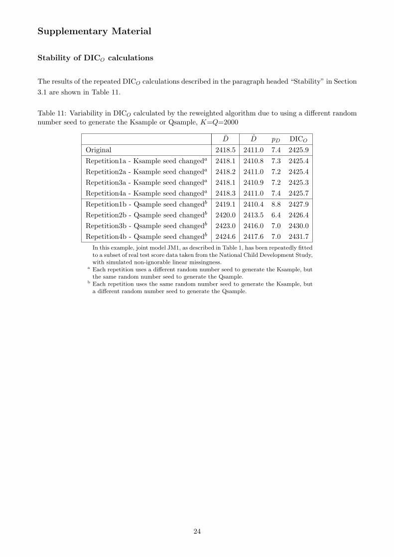
Stability

We would like the calculated value of DICO to be stable, and not depend on the random number

seed used to generate either the Ksample or Qsample. For an example based on data with simulated

missingness, we calculated DICO using the reweighted algorithm with K = 2, 000 and Q = 2, 000.

Firstly, we repeated the calculation four times, using different random number seeds for generating

the Ksample, but the same random number seed to generate the Qsample. The variation between the

DICO from the five calculations (original and four repetitions) was small (less that 1). Note that in

this case although the Qsample is generated from the same random number seed, it will also differ

between runs due to the Ksample differences. Secondly, we repeated the calculation another four

times, but using the same random number seed to generate the Ksample and four different random

number seeds for generating the Qsample. As the Ksample is generated from the same random number

8

seed, any differences are attributable to variation in the Qsample. Both D̄ and D̂ now exhibit much

larger variation, resulting in a difference between the highest and lowest DICO of about 6 which is

sufficiently large to be a concern, given that rules of thumb suggest that differences of 3-7 in DIC

should be regarded as important (Spiegelhalter et al., 2002). (These results are shown in Table 11 of

the Supplementary Material.) Repeating the exercise with Q increased to 10,000 lowered the variation

only slightly.

Using the algorithm without reweighting resulted in much greater stability of D̄, but D̂, and hence

DICO, remained variable. A method for assessing this instability is discussed in Section 3.3.

Computational time

One of the original reasons for using reweighting was to speed up the computation of DICO, since our

preferred method involves generating K + (K × Q) + Q samples, whereas the importance sampling

method just generates K + Q samples, and then reweights the single Q sample for every replicate

in the K sample. However, for equivalent sample sizes we found that our implementation of both

algorithms ran in about the same time, so there appears to be no computational advantage to using

reweighting in practice. This is because the computational time saved in the reweighting algorithm by

not generating the extra samples, is offset by evaluating the weights which also requires the calculation

of K ×Q model of interest likelihoods.

3.2 Choice of plug-in

As with calculating any DIC using posterior mean plug-ins, checks that these posterior means come

from approximately symmetric unimodal distributions are essential. One possibility is a visual inspec-

tion of the posterior distributions of the proposed plug-ins and a check that the coefficient of skewness,

where

coefficient of skewness =

1n

n∑i=1

(xi − x̄)3

sd(x)3, (9)

which is a measure of the asymmetry of a distribution, is close to 0.

3.3 Adequacy of the size of the Qsample

As discussed above (see paragraph headed “Stability” in Section 3.1), we would like to be sure that Q

is large enough to ensure that the DICO resulting from our calculations is stable. We have developed a

method for checking the stability of our results using subsets of the Qsample. These subsets are created

by splitting the complete Qsample in half, and then successively splitting the resulting subsets. D̄ and

D̂ for each subset and the full sample are then plotted against the size of the Qsample. (DICO could

also be plotted against Qsample size, but as it is a function of D̄ and D̂, it provides no additional

information.) The required extra calculations can be carried out with negligible additional cost in

running time.

Figure 1 provides examples of such plots, where Q = 40, 000 and the sample is repeatedly split

until a sample size of 2,500 is reached. This gives 2 non-overlapping Qsamples of length 20,000, 4

9

non-overlapping Qsamples of length 10,000, 8 non-overlapping Qsamples of length 5,000 and 16 non-

overlapping Qsamples of length 2,500. These plots show little variation in D̄ at each Q (all the crosses

are on top of each other), but a clear downwards trend as Q increases, which converges towards a limit.

However, D̂ exhibits instability for the plots labelled JM1 and especially for JM3, that decreases as

Q increases. (We will explain the stability in the JM2 plot in Section 4.) A similar downwards trend

to D̄, converging to a limit is indicated by the mean values of D̂.

We consider the Qsample size to be sufficient if our proposed deviance plot suggests both D̄ and D̂

have converged to a limit and D̂ has stabilised. On this basis 40,000 appears an adequate sample size

for calculating DICO for JM1, but a higher Q might produce a more accurate DICO for JM2 and JM3.

The plots for this and other synthetic examples suggest that higher variability and slower convergence

to a limit are associated with poorer fitting models.

4 Illustration of strategy on simulated data

In this section we illustrate our proposed strategy using simulated bivariate Normal data, and demon-

strate the inadequacies of using only DICO for comparing selection models with simulated time series

data.

4.1 Bivariate Normal data

We now assess how DICO and the missingness part of DICC can be used to help compare models,

using simulated data with simulated missingness so that the correct model is known. For this purpose,

we generate a dataset of bivariate Normal data with 1000 records comprising a response, y, and a

single covariate, x, s.t. (x

y

)∼ N

((0

1

),

(1 0.5

0.5 1

)). (10)

For this dataset the correct model of interest is

yi ∼ N(µi, σ2) (11)

µi = β0 + β1xi

and the true values of the parameters are β0 = 1 and β1 = 0.5.

We then delete some of the responses according to the equation pi = ϕ0 + ϕ1yi. The values of ϕ0 and

ϕ1 are chosen to impose linear non-ignorable missingness with a steep positive gradient, such that the

probability of being missing for the lowest value of y is 0 and the probability of being missing for the

highest value of y is 1. The chosen values also ensure that 0 ≤ pi ≤ 1 for all yi. Although the true

model of missingness is the linear equation pi = ϕ0 + ϕ1yi, this can be adequately modelled by the

linear logistic equation logit(pi) = θ0 + θ1yi, which ensures that the estimated probabilities always lie

in the range [0,1].

Our investigation is based on fitting four joint models (JM1-JM4), as specified in Table 1, to this

simulated dataset with simulated missingness. For JM1, we know that the specified model of interest

10

is correct and that the specified linear logit is a good approximation for the true model of missingness.

However, JM2 has an inadequate model of interest, JM3 has an incorrect error distribution and JM4

has too complex a model of missingness. So for the simulated data, we consider three different models

of interest and two different models of missingness. A full implementation of our proposed strategy

would involve fitting a set of joint models which pairs each model of interest with each model of

missingness (six joint models), and we do this in our real data application in Section 5.

Table 1: Specification of joint models for the bivariate Normal simulated data

Model Name Model of Interest Model of Missingness

JM1 yi ∼ N(µi, σ2); µi = β0 + β1xi logit(pi) = θ0 + θ1yi

JM2 yi ∼ N(µi, σ2); µi = β0 logit(pi) = θ0 + θ1yi

JM3 yi ∼ t4(µi, σ2); µi = β0 + β1xi logit(pi) = θ0 + θ1yi

JM4 yi ∼ N(µi, σ2); µi = β0 + β1xi logit(pi) = θ0 + θ1yi + θ2y

2i

Vague priors are specified for the unknown parameters of the model of interest: the β parameters are

assigned N(0,100002) priors and the precision, τ = 1σ2 , a Gamma(0.001,0.001) prior. Following Wake-

field (2004) and Jackson et al. (2006), we specify a logistic(0,1) prior for θ0 and a weakly informative

N(0,0.68) prior for θ1 and θ2, which corresponds to an approximately flat prior on the scale of pi.

We calculate the DICO for the three models with the same model of missingness (JM1, JM2 and JM3)

using the algorithm described in Section 3, with K = 2, 000 and Q = 40, 000. The likelihood for the

model of interest is calculated using

f(y|β) =(2πσ2

)−n2 exp

(− 1

2σ2

n∑i=1

(yi − µi)2

)for JM1&JM2

and f(y|β) =n∏

i=1

Γ(52

)2σ

√π

[1 +

(yi − µi

2σ

)2]− 5

2

for JM3.

In the t4 distribution σ is a scale parameter, s.t. σ =√

var2 , where var is the variance of the distribution.

For all three models, the likelihood for the model of missingness is calculated using

f(m|y,θ) =n∏

i=1

pmii (1− pi)

1−mi

where pi =eθ0+θ1yi

1 + eθ0+θ1yi.

The samples produced by the WinBUGS runs are from 2 chains of 15,000 iterations, with 10,000 burn-

in and the thinning parameter set to 5. Based on the Gelman-Rubin convergence statistic (Brooks

and Gelman, 1998) and a visual inspection of the chains, the WinBUGS runs required for calculating

DICO for the three models all converged.

As recommended in Section 3, we start by checking that the posterior means used as plug-ins come

from approximately symmetric unimodal distributions. From their coefficients of skewness (Equation

9) we find that the θ are skewed to some extent in all the models, and that the ymis are badly skewed

for JM3 (see Table 12 in the Supplementary Material for figures). However, as this simple example is

for illustration, we continue with these plug-ins, interpreting the DICO with caution.

11

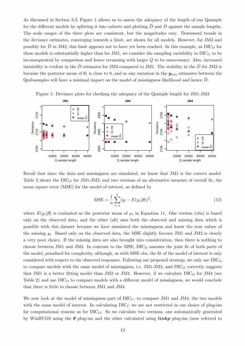
As discussed in Section 3.3, Figure 1 allows us to assess the adequacy of the length of our Qsample

for the different models by splitting it into subsets and plotting D̄ and D̂ against the sample lengths.

The scale ranges of the three plots are consistent, but the magnitudes vary. Downward trends in

the deviance estimates, converging towards a limit, are shown for all models. However, for JM3 and

possibly for D̄ in JM2, this limit appears not to have yet been reached. In this example, as DICO for

these models is substantially higher than for JM1, we consider the sampling variability in DICO to be

inconsequential by comparison and hence rerunning with larger Q to be unnecessary. Also, increased

instability is evident in the D̂ estimates for JM3 compared to JM1. The stability in the D̂ for JM2 is

because the posterior mean of θ1 is close to 0, and so any variation in the ymis estimates between the

Qsubsamples will have a minimal impact on the model of missingness likelihood and hence D̂.

Figure 1: Deviance plots for checking the adequacy of the Qsample length for JM1-JM3

10000 20000 30000 40000

2705

2715

2725

JM1

Q sample length

Dev

ianc

e

D

D̂mean D̂

10000 20000 30000 40000

2885

2895

2905

JM2

Q sample length

Dev

ianc

e

D

D̂mean D̂

10000 20000 30000 40000

2735

2745

2755

JM3

Q sample lengthD

evia

nce

D

D̂mean D̂

Recall that since the data and missingness are simulated, we know that JM1 is the correct model.

Table 2 shows the DICO for JM1-JM3, and two versions of an alternative measure of overall fit, the

mean square error (MSE) for the model of interest, as defined by

MSE =1

n

n∑i=1

(yi − E(yi|β))2, (12)

where E(yi|β) is evaluated as the posterior mean of µi in Equation 11. One version (obs) is based

only on the observed data, and the other (all) uses both the observed and missing data which is

possible with this dataset because we have simulated the missingness and know the true values of

the missing yi. Based only on the observed data, the MSE slightly favours JM1 and JM2 is clearly

a very poor choice. If the missing data are also brought into consideration, then there is nothing to

choose between JM1 and JM3. In contrast to the MSE, DICO assesses the joint fit of both parts of

the model, penalised for complexity, although, as with MSE obs, the fit of the model of interest is only

considered with respect to the observed responses. Following our proposed strategy, we only use DICO

to compare models with the same model of missingness, i.e. JM1-JM3, and DICO correctly suggests

that JM1 is a better fitting model than JM2 or JM3. However, if we calculate DICO for JM4 (see

Table 2) and use DICO to compare models with a different model of missingness, we would conclude

that there is little to choose between JM1 and JM4.

We now look at the model of missingness part of DICC , to compare JM1 and JM4, the two models

with the same model of interest. In calculating DICC we are not restricted in our choice of plug-ins

for computational reasons as for DICO. So we calculate two versions, one automatically generated

by WinBUGS using the θ plug-ins and the other calculated using linkp plug-ins (now referred to

12

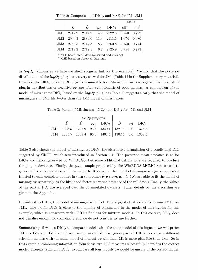
Table 2: Comparison of DICO and MSE for JM1-JM4

MSE

D̄ D̂ pD DICO alla obsb

JM1 2717.9 2712.9 4.9 2722.8 0.750 0.762

JM2 2900.3 2889.0 11.3 2911.6 1.074 0.980

JM3 2752.5 2744.3 8.2 2760.8 0.750 0.774

JM4 2719.2 2712.5 6.7 2725.9 0.754 0.773a MSE based on all data (observed and missing)b MSE based on observed data only

as logitp plug-ins as we have specified a logistic link for this example). We find that the posterior

distributions of the logitp plug-ins are very skewed for JM4 (Table 12 in the Supplementary material).

However, the DICC based on θ plug-ins is unusable for JM4 as it returns a negative pD. Very skew

plug-in distributions or negative pD are often symptomatic of poor models. A comparison of the

model of missingness DICC based on the logitp plug-ins (Table 3) suggests clearly that the model of

missingness in JM1 fits better than the JM4 model of missingness.

Table 3: Model of Missingness DICC and DIC8 for JM1 and JM4

logitp plug-ins

D̄ D̂ pD DICC D̂ pD DIC8

JM1 1323.5 1297.9 25.6 1349.1 1321.5 2.0 1325.5

JM4 1305.5 1209.4 96.0 1401.5 1302.5 3.0 1308.5

Table 3 also shows the model of missingness DIC8, the alternative formulation of a conditional DIC

suggested by CRFT, which was introduced in Section 2.4. The posterior mean deviance is as for

DICC and hence generated by WinBUGS, but some additional calculations are required to produce

the plug-in deviance. Firstly, the ymis sample produced by the WinBUGS MCMC run is used to

generate K complete datasets. Then using the R software, the model of missingness logistic regression

is fitted to each complete dataset in turn to produce θ̂(yobs,m,ymis). (We are able to fit the model of

missingness separately as the likelihood factorises in the presence of the full data.) Finally, the values

of the partial DIC are averaged over the K simulated datasets. Fuller details of this algorithm are

given in the Appendix.

In contrast to DICC , the model of missingness part of DIC8 suggests that we should favour JM4 over

JM1. The pD for DIC8 is close to the number of parameters in the model of missingness for this

example, which is consistent with CFRT’s findings for mixture models. In this context, DIC8 does

not penalise enough for complexity and we do not consider its use further.

Summarising, if we use DICO to compare models with the same model of missingness, we will prefer

JM1 to JM2 and JM3, and if we use the model of missingness part of DICC to compare different

selection models with the same model of interest we will find JM1 is more plausible than JM4. So in

this example, combining information from these two DIC measures successfully identifies the correct

model, whereas using only DICO to compare all four models we would be unsure of the correct model.

13

Before proceeding to our application, we consider some simulated longitudinal data which mimics the

basic structure of the clinical trial data that we will analyse in Section 5.

4.2 Time series data

For our second simulation we generate response data, yit, for i = 1, . . . , 1000 individuals at two time

points, t = 1, 2, using the random effects model:

yit ∼ N(µit, σ2)

µit = βi + ηt

βi ∼ N(γ, ρ2)

(13)

with σ = 1, η = −1, γ = 0 and ρ = 1. We then impose non-ignorable missingness on yi2 according

to the linear logistic equation, logit(pi) = yi2 − yi1, where pi is the probability that yi2 is missing. So

in this example, the missingness is dependent on the change in yi between time points. Three joint

models are fitted to this data, all with a correctly specified model of interest, as given by Equation 13,

but different models of missingness as specified in Table 4. The priors are similar to those specified for

the models in Section 4.1, and all the models exhibit satisfactory convergence. The model of interest

parameter estimates show that mnar2 is closest to fitting the true data generating model (see Table

13 in the Supplementary Material).

Table 4: Specification of the models of missingness for the simulated time series data

Model Name Model of Missingness equation

mar logit(piw) = θ0 + θ1yi1

mnar logit(piw) = θ0 + θ2yi2

mnar2 logit(piw) = θ0 + θ3yi1 + θ4(yi2 − yi1)

We calculate DICO for the three models as described in the previous section. Our recommended checks

show that the skewness in the posterior distributions of the plug-ins is acceptable and a Qsample length

of 40,000 is adequate (see Table 14 and Figure 4 in the Supplementary Material). In Section 2.3 we

discussed the limitations of DICO for comparing selection models with different models of missingness

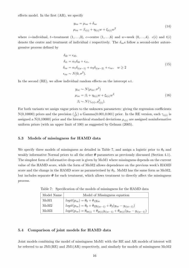
and recommended that DICO is not used for this purpose. Table 5 provides empirical support for this

recommendation, as the correct model (mnar2) clearly has the highest DICO. However, if instead we

use the model of missingness part of DICC , in line with our proposed strategy, we will conclude that

the mnar2 model best explains the missingness pattern regardless of the plug-ins chosen (Table 6).

Table 5: DICO for the simulated time series data

Model Name D̄ D̂ pD DICO

mar 5515.38 4788.26 727.12 6242.49

mnar 5462.65 4721.19 741.46 6204.12

mnar2 6003.97 5382.73 621.24 6625.21

These findings were replicated with two further datasets, randomly generated using the same equations,

14

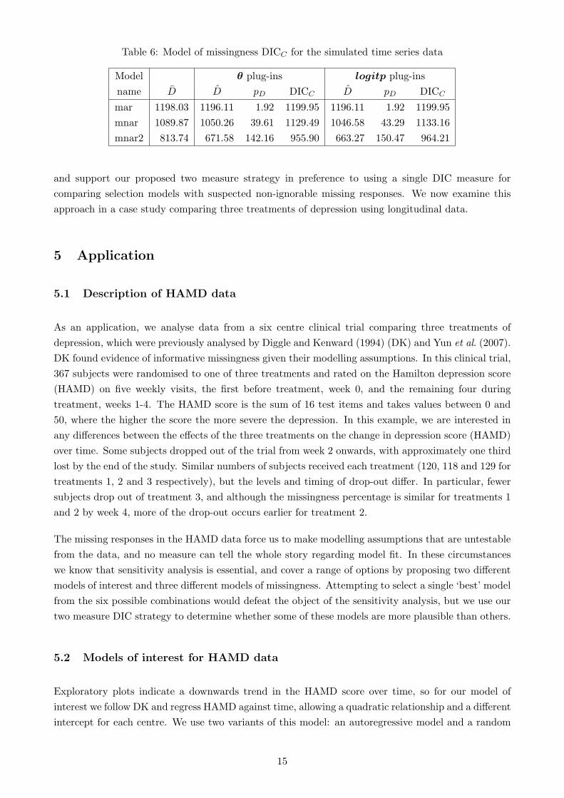
Table 6: Model of missingness DICC for the simulated time series data

Model θ plug-ins logitp plug-ins

name D̄ D̂ pD DICC D̂ pD DICC

mar 1198.03 1196.11 1.92 1199.95 1196.11 1.92 1199.95

mnar 1089.87 1050.26 39.61 1129.49 1046.58 43.29 1133.16

mnar2 813.74 671.58 142.16 955.90 663.27 150.47 964.21

and support our proposed two measure strategy in preference to using a single DIC measure for

comparing selection models with suspected non-ignorable missing responses. We now examine this

approach in a case study comparing three treatments of depression using longitudinal data.

5 Application

5.1 Description of HAMD data

As an application, we analyse data from a six centre clinical trial comparing three treatments of

depression, which were previously analysed by Diggle and Kenward (1994) (DK) and Yun et al. (2007).

DK found evidence of informative missingness given their modelling assumptions. In this clinical trial,

367 subjects were randomised to one of three treatments and rated on the Hamilton depression score

(HAMD) on five weekly visits, the first before treatment, week 0, and the remaining four during

treatment, weeks 1-4. The HAMD score is the sum of 16 test items and takes values between 0 and

50, where the higher the score the more severe the depression. In this example, we are interested in

any differences between the effects of the three treatments on the change in depression score (HAMD)

over time. Some subjects dropped out of the trial from week 2 onwards, with approximately one third

lost by the end of the study. Similar numbers of subjects received each treatment (120, 118 and 129 for

treatments 1, 2 and 3 respectively), but the levels and timing of drop-out differ. In particular, fewer

subjects drop out of treatment 3, and although the missingness percentage is similar for treatments 1

and 2 by week 4, more of the drop-out occurs earlier for treatment 2.

The missing responses in the HAMD data force us to make modelling assumptions that are untestable

from the data, and no measure can tell the whole story regarding model fit. In these circumstances

we know that sensitivity analysis is essential, and cover a range of options by proposing two different

models of interest and three different models of missingness. Attempting to select a single ‘best’ model

from the six possible combinations would defeat the object of the sensitivity analysis, but we use our

two measure DIC strategy to determine whether some of these models are more plausible than others.

5.2 Models of interest for HAMD data

Exploratory plots indicate a downwards trend in the HAMD score over time, so for our model of

interest we follow DK and regress HAMD against time, allowing a quadratic relationship and a different

intercept for each centre. We use two variants of this model: an autoregressive model and a random

15

effects model. In the first (AR), we specify

yiw = µiw + δiw

µiw = βc(i) + ηt(i)w + ξt(i)w2

(14)

where i=individual, t=treatment (1,. . . ,3), c=centre (1,. . . ,6) and w=week (0,. . . ,4). c(i) and t(i)

denote the centre and treatment of individual i respectively. The δiws follow a second-order autore-

gressive process defined by

δi0 = ϵi0,

δi1 = α1δi0 + ϵi1,

δiw = α1δi(w−1) + α2δi(w−2) + ϵiw, w ≥ 2

ϵiw ∼ N(0, σ2).

(15)

In the second (RE), we allow individual random effects on the intercept s.t.

yiw ∼ N(µiw, σ2)

µiw = βi + ηt(i)w + ξt(i)w2

βi ∼ N(γc(i), ρ2c(i)).

(16)

For both variants we assign vague priors to the unknown parameters: giving the regression coefficients

N(0,10000) priors and the precision ( 1σ2 ) a Gamma(0.001,0.001) prior. In the RE version, each γc(i) is

assigned a N(0,10000) prior and the hierarchical standard deviations ρc(i) are assigned noninformative

uniform priors (with an upper limit of 100) as suggested by Gelman (2005).

5.3 Models of missingness for HAMD data

We specify three models of missingness as detailed in Table 7, and assign a logistic prior to θ0 and

weakly informative Normal priors to all the other θ parameters as previously discussed (Section 4.1).

The simplest form of informative drop-out is given by MoM1 where missingness depends on the current

value of the HAMD score, while the form of MoM2 allows dependence on the previous week’s HAMD

score and the change in the HAMD score as parameterised by θ3. MoM3 has the same form as MoM2,

but includes separate θ for each treatment, which allows treatment to directly affect the missingness

process.

Table 7: Specification of the models of missingness for the HAMD data

Model Name Model of Missingness equation

MoM1 logit(piw) = θ0 + θ1yiw

MoM2 logit(piw) = θ0 + θ2yi(w−1) + θ3(yiw − yi(w−1))

MoM3 logit(piw) = θ0t(i) + θ2t(i)yi(w−1) + θ3t(i)(yiw − yi(w−1))

5.4 Comparison of joint models for HAMD data

Joint models combining the model of missingness MoM1 with the RE and AR models of interest will

be referred to as JM1(RE) and JM1(AR) respectively, and similarly for models of missingness MoM2

16

and MoM3. Runs of these six joint models and the models of interest estimated on complete cases

only, CC(RE) and CC(AR), converged based on the Gelman-Rubin convergence statistic and a visual

inspection of the chains. Adding a missingness model makes little difference to the β or γ estimates,

but there are substantial changes in some of the η and ξ parameters associated with the effect of

treatment over time. The impact of these changes will be assessed shortly using plots of the mean

response profiles for each treatment.

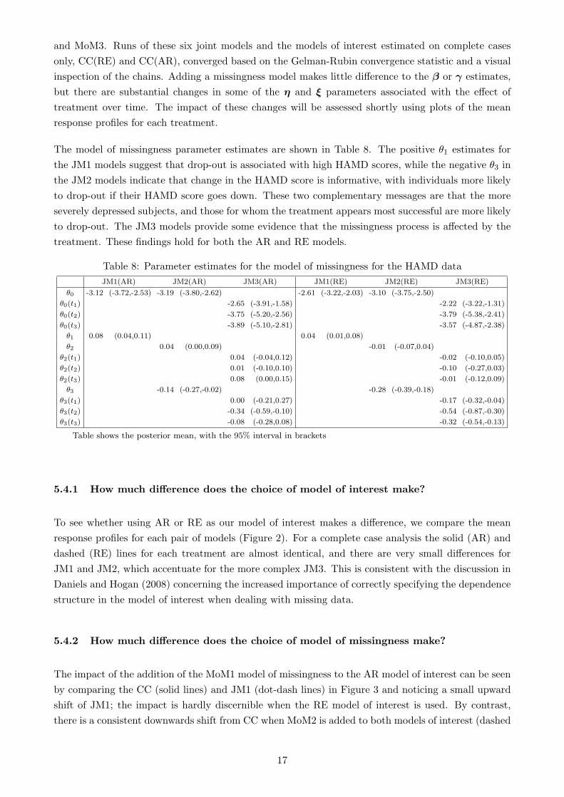
The model of missingness parameter estimates are shown in Table 8. The positive θ1 estimates for

the JM1 models suggest that drop-out is associated with high HAMD scores, while the negative θ3 in

the JM2 models indicate that change in the HAMD score is informative, with individuals more likely

to drop-out if their HAMD score goes down. These two complementary messages are that the more

severely depressed subjects, and those for whom the treatment appears most successful are more likely

to drop-out. The JM3 models provide some evidence that the missingness process is affected by the

treatment. These findings hold for both the AR and RE models.

Table 8: Parameter estimates for the model of missingness for the HAMD data

JM1(AR) JM2(AR) JM3(AR) JM1(RE) JM2(RE) JM3(RE)

θ0 -3.12 (-3.72,-2.53) -3.19 (-3.80,-2.62) -2.61 (-3.22,-2.03) -3.10 (-3.75,-2.50)

θ0(t1) -2.65 (-3.91,-1.58) -2.22 (-3.22,-1.31)

θ0(t2) -3.75 (-5.20,-2.56) -3.79 (-5.38,-2.41)

θ0(t3) -3.89 (-5.10,-2.81) -3.57 (-4.87,-2.38)

θ1 0.08 (0.04,0.11) 0.04 (0.01,0.08)

θ2 0.04 (0.00,0.09) -0.01 (-0.07,0.04)

θ2(t1) 0.04 (-0.04,0.12) -0.02 (-0.10,0.05)

θ2(t2) 0.01 (-0.10,0.10) -0.10 (-0.27,0.03)

θ2(t3) 0.08 (0.00,0.15) -0.01 (-0.12,0.09)

θ3 -0.14 (-0.27,-0.02) -0.28 (-0.39,-0.18)

θ3(t1) 0.00 (-0.21,0.27) -0.17 (-0.32,-0.04)

θ3(t2) -0.34 (-0.59,-0.10) -0.54 (-0.87,-0.30)

θ3(t3) -0.08 (-0.28,0.08) -0.32 (-0.54,-0.13)

Table shows the posterior mean, with the 95% interval in brackets

5.4.1 How much difference does the choice of model of interest make?

To see whether using AR or RE as our model of interest makes a difference, we compare the mean

response profiles for each pair of models (Figure 2). For a complete case analysis the solid (AR) and

dashed (RE) lines for each treatment are almost identical, and there are very small differences for

JM1 and JM2, which accentuate for the more complex JM3. This is consistent with the discussion in

Daniels and Hogan (2008) concerning the increased importance of correctly specifying the dependence

structure in the model of interest when dealing with missing data.

5.4.2 How much difference does the choice of model of missingness make?

The impact of the addition of the MoM1 model of missingness to the AR model of interest can be seen

by comparing the CC (solid lines) and JM1 (dot-dash lines) in Figure 3 and noticing a small upward

shift of JM1; the impact is hardly discernible when the RE model of interest is used. By contrast,

there is a consistent downwards shift from CC when MoM2 is added to both models of interest (dashed

17

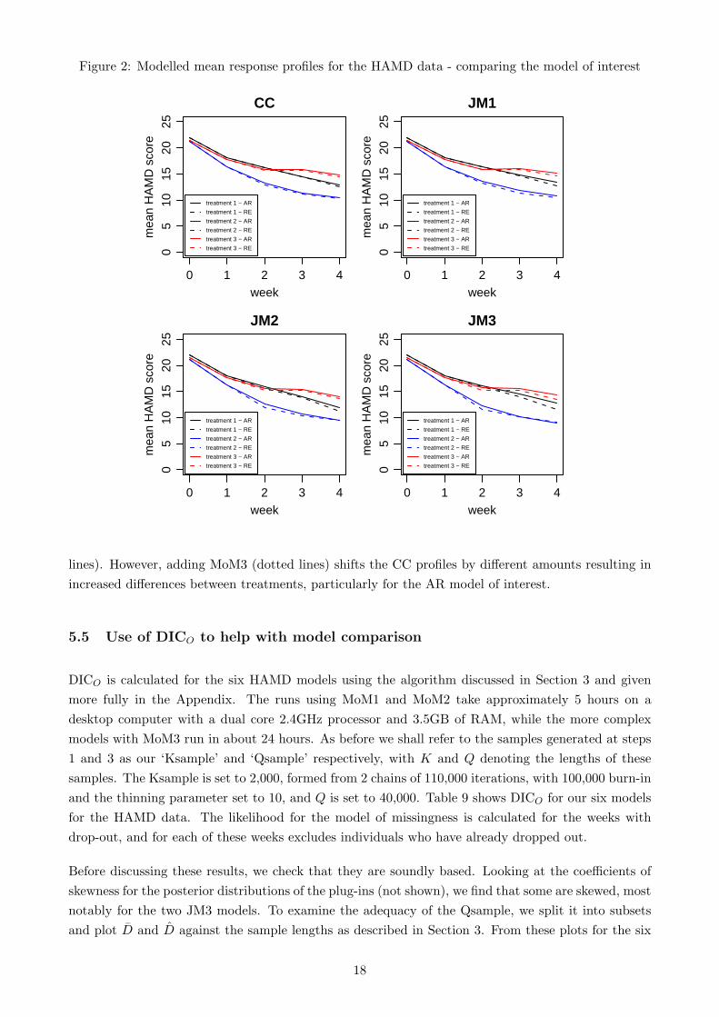
Figure 2: Modelled mean response profiles for the HAMD data - comparing the model of interest

0 1 2 3 4

05

1015

2025

CC

week

mea

n H

AM

D s

core

treatment 1 − AR

treatment 1 − RE

treatment 2 − AR

treatment 2 − RE

treatment 3 − AR

treatment 3 − RE

0 1 2 3 4

05

1015

2025

JM1

week

mea

n H

AM

D s

core

treatment 1 − AR

treatment 1 − RE

treatment 2 − AR

treatment 2 − RE

treatment 3 − AR

treatment 3 − RE

0 1 2 3 4

05

1015

2025

JM2

week

mea

n H

AM

D s

core

treatment 1 − AR

treatment 1 − RE

treatment 2 − AR

treatment 2 − RE

treatment 3 − AR

treatment 3 − RE

0 1 2 3 4

05

1015

2025

JM3

week

mea

n H

AM

D s

core

treatment 1 − AR

treatment 1 − RE

treatment 2 − AR

treatment 2 − RE

treatment 3 − AR

treatment 3 − RE

lines). However, adding MoM3 (dotted lines) shifts the CC profiles by different amounts resulting in

increased differences between treatments, particularly for the AR model of interest.

5.5 Use of DICO to help with model comparison

DICO is calculated for the six HAMD models using the algorithm discussed in Section 3 and given

more fully in the Appendix. The runs using MoM1 and MoM2 take approximately 5 hours on a

desktop computer with a dual core 2.4GHz processor and 3.5GB of RAM, while the more complex

models with MoM3 run in about 24 hours. As before we shall refer to the samples generated at steps

1 and 3 as our ‘Ksample’ and ‘Qsample’ respectively, with K and Q denoting the lengths of these

samples. The Ksample is set to 2,000, formed from 2 chains of 110,000 iterations, with 100,000 burn-in

and the thinning parameter set to 10, and Q is set to 40,000. Table 9 shows DICO for our six models

for the HAMD data. The likelihood for the model of missingness is calculated for the weeks with

drop-out, and for each of these weeks excludes individuals who have already dropped out.

Before discussing these results, we check that they are soundly based. Looking at the coefficients of

skewness for the posterior distributions of the plug-ins (not shown), we find that some are skewed, most

notably for the two JM3 models. To examine the adequacy of the Qsample, we split it into subsets

and plot D̄ and D̂ against the sample lengths as described in Section 3. From these plots for the six

18

Figure 3: Modelled mean response profiles for the HAMD data - comparing the model of missingness

0 1 2 3 4

05

1015

2025

AR

week

mea

n H

AM

D s

core

treat 1 − CC

treat 1 − JM1

treat 1 − JM2

treat 1 − JM3

treat 2 − CC

treat 2 − JM1

treat 2 − JM2

treat 2 − JM3

treat 3 − CC

treat 3 − JM1

treat 3 − JM2

treat 3 − JM3

0 1 2 3 4

05

1015

2025

RE

weekm

ean

HA

MD

sco

re

treat 1 − CC

treat 1 − JM1

treat 1 − JM2

treat 1 − JM3

treat 2 − CC

treat 2 − JM1

treat 2 − JM2

treat 2 − JM3

treat 3 − CC

treat 3 − JM1

treat 3 − JM2

treat 3 − JM3

In the AR plot, the CC and JM3 lines for treatment 1 are almost coincident. In the RE plot, the CC and JM1 lines arealmost coincident for all treatments, and the JM2 and JM3 lines for treatment 3 are almost coincident.

Table 9: DICO for the HAMD data

θ plug-ins

D̄ D̂ pD DICO

JM1(AR) 9995.8 9978.6 17.2 10013.0

JM1(RE) 9663.2 9359.6 303.7 9966.9

JM2(AR) 9991.0 9965.5 25.5 10016.5

JM2(RE) 9680.6 9372.6 308.0 9988.5

JM3(AR) 9995.1 9965.0 30.1 10025.2

JM3(RE) 9698.1 9392.1 306.0 10004.2

models (shown as Figure 5 in the Supplementary Material), we see that both D̄ and D̂ are stable and

show little variation even for small Q for both JM1 models. For the other models, trends similar to

those exhibited by our synthetic data (see Figure 1) are evident, but again there is convergence to a

limit suggesting the adequacy of Q=40,000. As before, we also see that the instability associated with

small Q decreases with increased sample size. The trends and variation are more pronounced for the

RE models than the AR models.

Our investigation with simulated data suggests that DICO can give useful information about the

relative merits of the model of interest. For the HAMD example, DICO provides consistent evidence

that the random effects model of interest is preferable to the autoregressive model of interest when

combined with each model of missingness, as can be seen by DICO always being smaller for RE than

AR for each of the three models of missingness.

19

5.6 Use of the model of missingness DICC to help with model comparison

We now turn to the model of missingness part of DICC , to see what additional information it provides.

Table 10 shows two versions, one based on the θ plug-ins and one on the logitp plug-ins. As with

the θ plug-ins, the posterior distributions of the logitp plug-ins become increasingly skewed as the

model of missingness becomes more complex. We have reservations about both sets of plug-ins, but

find that they provide a consistent message from the model of missingness DICC . MoM2 and MoM3,

used in the JM2 and JM3 models, provide clearly a better fit to this part of the model than JM1,

with an edge towards JM3 rather than JM2, i.e. a missingness model that allows treatment specific

parameters.

Table 10: Model of missingness DICC for the HAMD data

θ plug-ins logitp plug-ins

D̄ D̂ pD DICC D̂ pD DICC

JM1(AR) 698.6 695.5 3.1 701.8 694.3 4.3 703.0

JM2(AR) 653.4 649.5 3.9 657.3 636.5 16.9 670.2

JM3(AR) 626.0 621.8 4.2 630.2 583.1 42.9 668.9

JM1(RE) 719.6 717.8 1.9 721.5 716.3 3.3 723.0

JM2(RE) 547.5 517.7 29.8 577.3 511.2 36.3 583.8

JM3(RE) 521.6 480.4 41.2 562.8 464.6 57.0 578.6

5.7 Combined use of DICO and the model of missingness DICC

To conclude, within this sensitivity analysis, DICO suggests that the RE model of interest is more

plausible than the AR. For RE models, there are substantial improvements in the model of missingness

DICC for JM2 and JM3 over JM1, i.e. JM2 and JM3 better explain the missingness pattern than JM1.

Overall, of the joint models explored, those with a RE model of interest and a model of missingness

that depends on the change in HAMD (either treatment specific or not) seem most appropriate for

the HAMD data.

If we based our analysis of this clinical trial data on a complete case analysis, we would conclude that

treatment 2 lowers the HAMD score more than treatments 1 and 3 throughout the trial, and treatment

1 is more successful than treatment 3 in lowering HAMD in the later weeks. The same conclusions are

reached using our preferred joint models, i.e. JM2(RE) and JM3(RE), but all the treatments appear

a little more effective in lowering HAMD (compare the dotted and dashed lines with the solid lines in

the RE plot of Figure 3).

6 Discussion

For complete data, DIC is routinely used by Bayesian statisticians to compare models, a practice

facilitated by its automatic generation in WinBUGS. However, using DIC in the presence of missing

20

data is far from straightforward. The usual issues surrounding the choice of plug-ins are heightened,

and in addition we must ensure that its construction is sensible. No single measure of DIC, or indeed

combination of measures, can provide a full picture of model fit since we can never evaluate fit to the

missing data. However, the use of two complementary measures can provide more information than

one DIC measure used in isolation. The model comparison strategy that we have developed relies on

using both DICO and the model of missingness part of DICC . A DIC based on the observed data

likelihood, DICO, can help with the choice of the model of interest, and should be used to compare

joint models built with the same model of missingness but different models of interest. The model

of missingness part of DICC , which uses information provided by the missingness indicators, allows

comparison of the fit of different models of missingness for selection models with the same model of

interest.

DICO cannot be generated by WinBUGS, but can be calculated from WinBUGS output using other

software. DH provide an algorithm for its calculation, which we have adapted and implemented for

both simulated and real data examples. We recommend performing two sets of checks: (1) that the

plug-ins are reasonable (i.e. if posterior means are used, they should come from symmetric, unimodal

posterior distributions, and they must ensure consistency in the calculation of the posterior mean

deviance and the plug-in deviance, so that missing values are integrated out in both parts of the DIC)

and (2) that the size of the samples generated from the likelihoods (Qsamples) is sufficiently large to

avoid overestimating DICO and problems with instability in the plug-in deviance (we suggest plotting

deviance against sample length and checking for stability, as in Figure 1). Based on limited exploration

of synthetic and real data, we tentatively propose working with a Qsample of at least 40,000. Again

based on our experience, we tentatively suggest that even with a well chosen Qsample size, a DIC

difference of at least 5 is required to provide some evidence of a genuine difference in the fit of two

models, as opposed to reflecting sampling variability.

A model’s fit to the observed data can be assessed, but its fit to the unobserved data given the

observed data cannot be assessed. So, in using DICO we must remember that it will only tell us about

the fit of our model to the observed data and nothing about the fit to the missing data. However,

it does seem reasonable to use it to compare joint models with different models of interest but the

same models of missingness. DH discussed an alternative construction (DICF ) for selection models

based on the posterior predictive expectation of the full data likelihood, L(β,θ|yobs,ymis,m), and

provided a broad outline for its implementation. DICF may provide additional information for model

comparison, but its calculation is complicated as the expectation for the plug-ins is conditional on

ymis. We have found it to be computationally very unstable in preliminary investigations (DH also

noted similar computational problems; personal communication).

An alternative to using DIC to compare models, is to assess model fit using a set of data not used in

the model estimation, if available. In surveys, sometimes data is collected from individuals who are

originally non-contacts or refusals, and using this for comparing model fit is particularly attractive

as such individuals are likely to be similar to those who have missing data. By contrast, alternatives

such as K-fold validation will only tell us about the fit to the observed data and as such provide an

alternative to the DICO part of the strategy. The link between cross-validation and DIC is discussed

by Plummer (2008).

Although the DICO and model of missingness DICC can provide complementary, useful insights into

21

the comparative fit of various selection models, it would be a mistake to use them to select a single

model. Rather our strategy should be viewed as a screening method that can help us to identify

plausible models. Even with straightforward data, such as our first simulated example, the usual

plug-ins are affected by skewness. This skewness makes the interpretation of DIC more complicated,

as we have to allow for some additional variability that can obscure the message from the proposed

strategy. Given this and the lack of knowledge regarding the fit of the missing data, we emphasise that

DIC should never be used in isolation. Our DIC strategy should be used in the context of a sensitivity

analysis, designed to check that conclusions are robust to a range of assumptions about the missing

data. In summary, our investigations have shown that these two DIC measures have the potential to

assist in the selection of a range of plausible models which have a reasonable fit to quantities that can

be checked and allow the uncertainty introduced by non-ignorable missing data to be propagated into

conclusions about a question of interest.

Appendix

Algorithm for calculating DICO

Our preferred algorithm for calculating DICO proceeds as follows: (f(y|β, σ) is the model of interest,

typically Normal or t in our applications, and f(m|y,θ) is a Bernoulli model of missingness in a

selection model)

1 Carry out a standard MCMC run on the joint model f(y,m|β, σ,θ). Save samples of β, σ and θ,

denoted by β(k), σ(k) and θ(k), k = 1, . . . ,K, which we shall call the Ksample.

2 Evaluate the posterior means of β, σ and θ, denoted by β̂, σ̂ and θ̂. (Evaluate σ̂ on the log

scale and then back transform, see discussion headed “Skewness in the plug-ins for the simulated

example” in the Supplementary Material for rationale.)

3 For each member of the Ksample, generate a sample y(kq)mis , q = 1, . . . , Q, from the appropriate

likelihood evaluated at β(k) and σ(k), e.g. ykmis ∼ N(Xβ(k), σ(k)2). We denote the sample associated

with member k of the Ksample as Qsample(k).

4 Then evaluate

h(k) = Eymis|yobs,β(k),σ(k){f(m|yobs,ymis,θ(k))} ≈ 1

Q

Q∑q=1

f(m|yobs,y(kq)mis ,θ

(k)).

Calculate the posterior expectation of the observed data log likelihood as

logL(β, σ,θ|yobs,m) ≈ 1

K

K∑k=1

[logL(β(k), σ(k)|yobs) + log h(k)

].

Multiply this by -2 to get the posterior mean of the deviance, denoted D̄.

5 Generate a new Qsample, y(q)mis, q = 1, . . . , Q, using β̂ and σ̂. Evaluate the plug-in observed data

log likelihood using the posterior means from the Ksample as

logL(β, σ,θ|yobs,m) ≈ logL(β̂, σ̂|yobs) + log(Eymis|yobs,β̂,σ̂

{f(m|yobs,ymis, θ̂)})

22

where

Eymis|yobs,β̂,σ̂{f(m|yobs,ymis, θ̂)} ≈ 1

Q

Q∑q=1

f(m|yobs,y(q)mis, θ̂).

Multiply this plug-in log likelihood by -2 to get the plug-in deviance, denoted D̂.

6 Finally, calculate DICO = 2D̄ − D̂.

To implement an algorithm using reweighting as proposed by DH, alter steps 3-5 as follows:

3 Generate a Qsample y(q)mis, q = 1, . . . , Q, from the appropriate likelihood evaluated at the posterior

means, e.g. ymis ∼ N(Xβ̂, σ̂2) (as in step 5 of our preferred algorithm).

4 For each value of (β(k), σ(k)) in the Ksample, and each value of y(q)mis from the Qsample, calculate

the weight

w(k)q =

f(y(q)mis|yobs,β

(k), σ(k))

f(y(q)mis|yobs, β̂, σ̂)

.

and evaluate

h(k) = Eymis|yobs,β(k),σ(k){f(m|yobs,ymis,θ(k))} ≈

Q∑q=1

w(k)q f(m|yobs,y

(q)mis,θ

(k))

Q∑q=1

w(k)q

.

Calculate the posterior expectation of the observed data log likelihood and D̄ as before.

5 There is no need to generate a further Qsample, simply use the Qsample generated at the replace-

ment step 3 to evaluate the plug-in observed data log likelihood and D̂ as before.

Algorithm for calculating the plug-in deviance for the model of missingness part

of DIC8

1 Carry out a standard MCMC run on the joint model f(y,m|β, σ,θ). Save samples of ymis, denoted

by y(k)mis, k = 1, . . . ,K, and use these to form K complete datasets.

2 Fit the model of missingness part of the joint model, f(m|y,θ), to each complete dataset to

calculate θ̂(yobs,m,ymis).

3 Then average results from the K datasets to get the plug-in log likelihood:

Eymis|yobs,m{logf(m|yobs,ymis, θ̂(yobs,m,ymis))} ≈ 1

K

K∑k=1

[logf(m|yobs,y

(k)mis, θ̂(yobs,m,y

(k)mis))

].

Multiply this plug-in log likelihood by -2 to get the plug-in deviance.

Acknowledgements

Financial support: this work was supported by an ESRC PhD studentship (Alexina Mason). Sylvia

Richardson and Nicky Best would like to acknowledge support from ESRC: RES-576-25-5003 and

RES-576-25-0015. The authors are grateful to Mike Kenward for useful discussions and providing the

clinical trial data analysed in this paper. Alexina Mason thanks Ian Plewis for his encouragement

during her research on non-ignorable missing data.

23

Supplementary Material

Stability of DICO calculations

The results of the repeated DICO calculations described in the paragraph headed “Stability” in Section

3.1 are shown in Table 11.

Table 11: Variability in DICO calculated by the reweighted algorithm due to using a different randomnumber seed to generate the Ksample or Qsample, K=Q=2000

D̄ D̂ pD DICO

Original 2418.5 2411.0 7.4 2425.9

Repetition1a - Ksample seed changeda 2418.1 2410.8 7.3 2425.4

Repetition2a - Ksample seed changeda 2418.2 2411.0 7.2 2425.4

Repetition3a - Ksample seed changeda 2418.1 2410.9 7.2 2425.3

Repetition4a - Ksample seed changeda 2418.3 2411.0 7.4 2425.7

Repetition1b - Qsample seed changedb 2419.1 2410.4 8.8 2427.9

Repetition2b - Qsample seed changedb 2420.0 2413.5 6.4 2426.4

Repetition3b - Qsample seed changedb 2423.0 2416.0 7.0 2430.0

Repetition4b - Qsample seed changedb 2424.6 2417.6 7.0 2431.7

In this example, joint model JM1, as described in Table 1, has been repeatedly fittedto a subset of real test score data taken from the National Child Development Study,with simulated non-ignorable linear missingness.

a Each repetition uses a different random number seed to generate the Ksample, butthe same random number seed to generate the Qsample.

b Each repetition uses the same random number seed to generate the Ksample, buta different random number seed to generate the Qsample.

24

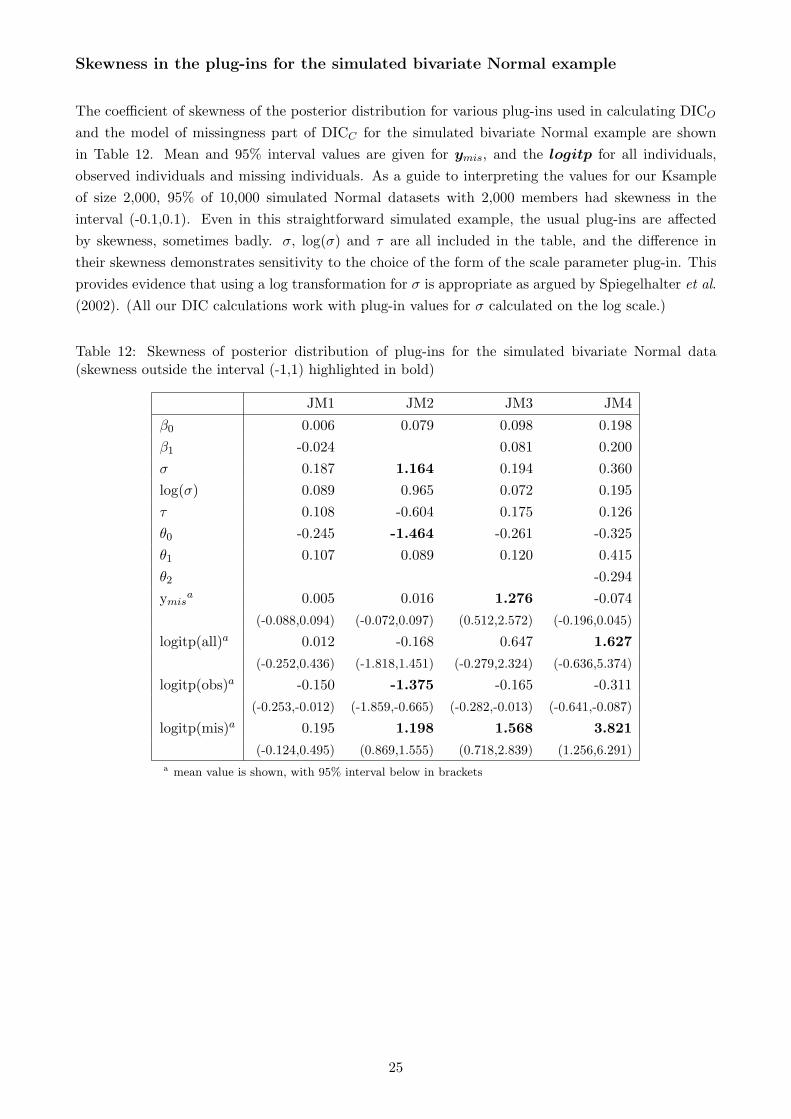
Skewness in the plug-ins for the simulated bivariate Normal example

The coefficient of skewness of the posterior distribution for various plug-ins used in calculating DICO

and the model of missingness part of DICC for the simulated bivariate Normal example are shown

in Table 12. Mean and 95% interval values are given for ymis, and the logitp for all individuals,

observed individuals and missing individuals. As a guide to interpreting the values for our Ksample

of size 2,000, 95% of 10,000 simulated Normal datasets with 2,000 members had skewness in the

interval (-0.1,0.1). Even in this straightforward simulated example, the usual plug-ins are affected

by skewness, sometimes badly. σ, log(σ) and τ are all included in the table, and the difference in

their skewness demonstrates sensitivity to the choice of the form of the scale parameter plug-in. This

provides evidence that using a log transformation for σ is appropriate as argued by Spiegelhalter et al.

(2002). (All our DIC calculations work with plug-in values for σ calculated on the log scale.)

Table 12: Skewness of posterior distribution of plug-ins for the simulated bivariate Normal data(skewness outside the interval (-1,1) highlighted in bold)

JM1 JM2 JM3 JM4

β0 0.006 0.079 0.098 0.198

β1 -0.024 0.081 0.200

σ 0.187 1.164 0.194 0.360

log(σ) 0.089 0.965 0.072 0.195

τ 0.108 -0.604 0.175 0.126

θ0 -0.245 -1.464 -0.261 -0.325

θ1 0.107 0.089 0.120 0.415

θ2 -0.294

ymisa 0.005 0.016 1.276 -0.074

(-0.088,0.094) (-0.072,0.097) (0.512,2.572) (-0.196,0.045)

logitp(all)a 0.012 -0.168 0.647 1.627

(-0.252,0.436) (-1.818,1.451) (-0.279,2.324) (-0.636,5.374)

logitp(obs)a -0.150 -1.375 -0.165 -0.311

(-0.253,-0.012) (-1.859,-0.665) (-0.282,-0.013) (-0.641,-0.087)

logitp(mis)a 0.195 1.198 1.568 3.821

(-0.124,0.495) (0.869,1.555) (0.718,2.839) (1.256,6.291)a mean value is shown, with 95% interval below in brackets

25

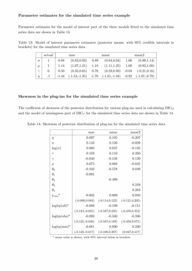
Parameter estimates for the simulated time series example

Parameter estimates for the model of interest part of the three models fitted to the simulated time

series data are shown in Table 13.

Table 13: Model of interest parameter estimates (posterior means, with 95% credible intervals inbrackets) for the simulated time series data

actual mar mnar mnar2

σ 1 0.88 (0.83,0.93) 0.89 (0.84,0.94) 1.06 (0.99,1.14)

ρ 1 1.14 (1.07,1.21) 1.18 (1.11,1.25) 1.00 (0.92,1.08)

γ 0 0.50 (0.35,0.65) 0.76 (0.59,0.93) -0.03 (-0.21,0.16)

η -1 -1.44 (-1.53,-1.35) -1.70 (-1.81,-1.58) -0.92 (-1.07,-0.78)

Skewness in the plug-ins for the simulated time series example

The coefficient of skewness of the posterior distribution for various plug-ins used in calculating DICO

and the model of missingness part of DICC for the simulated time series data are shown in Table 14.

Table 14: Skewness of posterior distribution of plug-ins for the simulated time series data

mar mnar mnar2

η 0.097 0.105 -0.207

σ 0.143 0.126 -0.029

log(σ) 0.060 0.047 -0.135

τ 0.103 0.110 0.350

γ -0.040 -0.138 0.129

ρ 0.075 0.068 -0.045

θ0 -0.103 -0.578 0.049

θ1 -0.091

θ2 -0.499

θ3 0.249

θ4 0.283

ymisa -0.002 0.009 0.050

(-0.090,0.083) (-0.114,0.122) (-0.121,0.205)

logitp(all)a -0.089 -0.199 -0.151

(-0.124,-0.031) (-0.587,0.235) (-0.450,0.352)

logitp(obs)a -0.093 -0.340 -0.336

(-0.125,-0.040) (-0.587,0.189) (-0.458,0.071)

logitp(mis)a -0.081 0.090 0.230

(-0.122,-0.017) (-0.100,0.287) (0.047,0.417)a mean value is shown, with 95% interval below in brackets

26

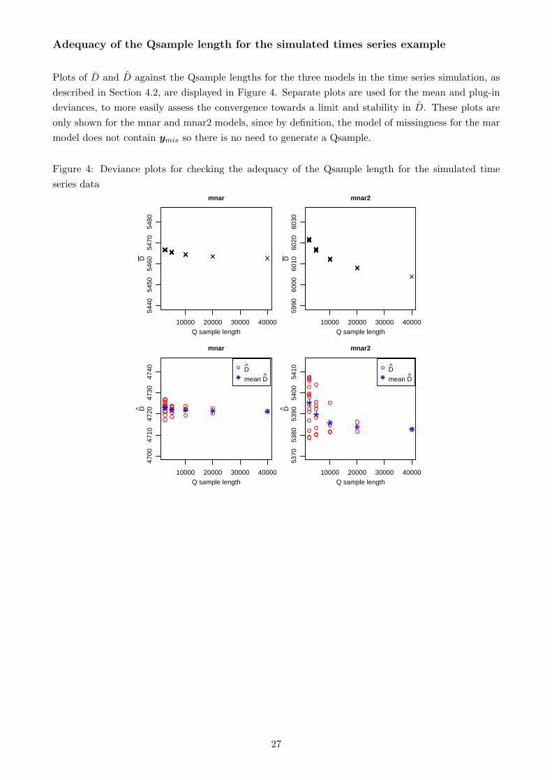
Adequacy of the Qsample length for the simulated times series example

Plots of D̄ and D̂ against the Qsample lengths for the three models in the time series simulation, as

described in Section 4.2, are displayed in Figure 4. Separate plots are used for the mean and plug-in

deviances, to more easily assess the convergence towards a limit and stability in D̂. These plots are

only shown for the mnar and mnar2 models, since by definition, the model of missingness for the mar

model does not contain ymis so there is no need to generate a Qsample.

Figure 4: Deviance plots for checking the adequacy of the Qsample length for the simulated time

series data

10000 20000 30000 40000

5440

5450

5460

5470

5480

mnar

Q sample length

D

10000 20000 30000 40000

5990

6000

6010

6020

6030

mnar2

Q sample length

D

10000 20000 30000 40000

4700

4710

4720

4730

4740

mnar

Q sample length

D̂

D̂

mean D̂

10000 20000 30000 40000

5370

5380

5390

5400

5410

mnar2

Q sample length

D̂

D̂

mean D̂

27

Adequacy of the Qsample length for the HAMD example

Plots of D̄ and D̂ against the Qsample lengths for the six models in the HAMD example, as described

in Section 5.5, are displayed in Figure 5. The mean and plug-in deviances are shown on the same plot

for the AR models, but separate plots are used for the RE models, where the difference between the

two deviances is much larger, to maintain consistent scales.

Figure 5: Deviance plots for checking the adequacy of the Qsample length for the HAMD data

10000 20000 30000 40000

9950

9970

9990

JM1(AR2)

Q sample length

Dev

ianc

e

D

D̂mean D̂

10000 20000 30000 40000

9950

9970

9990

JM2(AR2)

Q sample length

Dev

ianc

e

D

D̂mean D̂

10000 20000 30000 40000

9950

9970

9990

JM3(AR2)

Q sample length

Dev

ianc

e

D

D̂mean D̂

10000 20000 30000 40000

9660

9680

9700

JM1(RE)

Q sample length

D

10000 20000 30000 40000

9660

9680

9700

JM2(RE)

Q sample length

D

10000 20000 30000 40000

9660

9680

9700

JM3(RE)

Q sample length

D

10000 20000 30000 40000

9350

9370

9390

JM1(RE)

Q sample length

D̂

D̂

mean D̂

10000 20000 30000 40000

9350

9370

9390

JM2(RE)

Q sample length

D̂

D̂

mean D̂

10000 20000 30000 40000

9370

9390

9410

JM3(RE)

Q sample length

D̂

D̂

mean D̂

28

References

Brooks, S. and Gelman, A. (1998). General Methods for Monitoring Convergence of Iterative Simula-

tions. Journal of Computational and Graphical Statistics, 7, 434–55.

Celeux, G., Forbes, F., Robert, C. P., and Titterington, D. M. (2006). Deviance Information Criteria

for Missing Data Models. Bayesian Analysis, 1, (4), 651–74.

Daniels, M. J. and Hogan, J. W. (2008). Missing Data In Longitudinal Studies Strategies for Bayesian

Modeling and Sensitivity Analysis. Chapman & Hall.

Dempster, A. P. (1973). The direct use of likelihood for significance testing. In Proceedings of Con-

ference on Foundational Questions in Statistical Inference, (ed. O. Barndorff-Nielsen, P. Blaesild,

and G. Schou), pp. 335–54. University of Aarhus.

Dempster, A. P. (1997). The direct use of likelihood for significance testing. Statistics and Computing,

7, 247–52.

Diggle, P. and Kenward, M. G. (1994). Informative Drop-out in Longitudinal Data Analysis (with

discussion). Journal of the Royal Statistical Society, Series C (Applied Statistics), 43, (1), 49–93.

Fitzmaurice, G. M. (2003). Methods for Handling Dropouts in Longitudinal Clinical Trials. Statistica

Neerlandica, 57, (1), 75–99.

Gelman, A. (2005). Prior distributions for variance parameters in hierarchical models. Bayesian

Analysis, 1, (2), 1–19.

Gelman, A., Carlin, J. B., Stern, H. S., and Rubin, D. B. (2004). Bayesian Data Analysis, (2nd edn).

Chapman & Hall.

Jackson, C., Best, N., and Richardson, S. (2006). Improving ecological inference using individual-level

data. Statistics in Medicine, 25, 2136–59.

Kenward, M. G. and Molenberghs, G. (1999). Parametric models for incomplete continuous and

categorical longitudinal data. Statistical Methods in Medical Research, 8, (1), 51–83.

Liu, J. S. (2001). Monte Carlo Strategies in Scientific Computing, (1st edn). Springer-Verlag.

Michiels, B., Molenberghs, G., Bijnens, L., Vangeneugden, T., and Thijs, H. (2002). Selection mod-

els and pattern-mixture models to analyse longitudinal quality of life data subject to drop-out.

Statistics in Medicine, 21, 1023–41.

Peruggia, M. (1997). On the Variability of Case-Deletion Importance Sampling Weights in the

Bayesian Linear Model. Journal of the American Statistical Association, 437, (92), 199–207.

Plummer, M. (2008). Penalized loss functions for Bayesian model comparison. Biostatistics, 9, (3),

523–39.

Schafer, J. L. and Graham, J. W. (2002). Missing Data: Our View of the State of the Art. Psychological

Methods, 7, (2), 147–77.

Spiegelhalter, D. J., Best, N. G., Carlin, B. P., and van der Linde, A. (2002). Bayesian measures

of model complexity and fit (with discussion). Journal of the Royal Statistical Society, Series B

(Statistical Methodology), 64, (4), 583–639.

Spiegelhalter, D. J., Thomas, A., Best, N. G., and Lunn, D. (2003). WinBUGS Version 1.4 User

Manual. MRC Biostatistics Unit, Cambridge, Available from www.mrc-bsu.cam.ac.uk/bugs.

Wakefield, J. (2004). Ecological inference for 2 x 2 tables. Journal of the Royal Statistical Society,

Series A (Statistics in Society), 167, (3), 385–445.

Yun, S.-C., Lee, Y., and Kenward, M. G. (2007). Using hierarchical likelihood for missing data

problems. Biometrika, 94, (4), 905–19.

29