Assessing the Assumption of Strongly Ignorable Treatment

Assignment Under Assumed Causal Models

Takeshi Emura, Jingfang Wang and Hitomi Katsuyama∗

April 23, 2008

Abstract

The assumption of strong ignorability is imposed by most inference methods for

estimating the treatment effect in observational studies. We propose a likelihood ratio

test for checking this important assumption. Simulations are conducted to investigate

the performance of the proposed method. We demonstrate the proposed method using

data from an observational study for measuring English educational effect on Japanese

elementary school students.

KEY WORDS: Counterfactual model of causality; Independence test; Likelihood ratio

test; Missing data; Model checking; Propensity score

∗Takeshi Emura is Assistant Professor, Division of Biostatistics, School of Pharmaceutical Sciences,

Kitasato University, 5-9-1, Sirokane, Minato-ku, Japan, Jingfang Wang is Associate Professor, Faculty of

Sciences, Chiba University, 1-33, Yayoi-cho, Inageku, Chiba-shi, Japan, and Hitomi Katsuyama is Lecturer,

Department of English, Kawamura Gakuen Women’s University, 1133 Sageto Abiko-shi, Chiba, Japan

1

1 INTRODUCTION

Observational studies are often used to study the effect of a treatment when it is not fea-

sible to use controlled experiment. Since the original work of Cochran (1965), substantial

research efforts have been devoted to developing methodologies suited for observational

studies. Rosenbaum (2002) summarizes the concepts of observational studies with a for-

mal mathematical framework, illustrated with plenty of real examples. Applications of

observational studies arise in biology, econometrics, education and sociology to name but

a few. Dehejia and Wahba (1999) studied the effect of a labor training program in the

United States. They compared the after-intervention income of the program participants

with that of non-participants using a database. In a series of papers of Coleman, Hoffer

and Kilgore (1982), Goldberger and Cain (1982) and Morgan (2001), the effect of at-

tending Catholic schools, compared to private and public schools, has been studied under

non-experimental setting. In Japan, the efficacy of early introduction of English training

program is of substantial interest to both the general public and the government (Kat-

suyama, Nishigaki and Wang 2006). In Section 5.2, we consider a study on the effect

of English educational program in School A in Chiba prefecture, Japan, based on data

collected by the authors. In most observational studies, the typical focus of interest is the

effect of treatment, such as the efficacies of training programs or medical treatments.

A modern approach to investigating the treatment effect in observational studies is

based on the counterfactual models of causality. Although some model assumptions are

necessary, the counterfactual models do provide a systematic way to define the treat-

ment effect. Specifically, the successful development in both theory and application on

propensity score (Rosenbaum and Rubin 1983) increased the value of the counterfactual

modeling. Rosenbaum and Rubin (1983) reviews how the point estimates for the treat-

ment effect can be constructed based on stratification and matching on propensity scores.

In recent years, the counterfactual models have been adopted by many researchers who

aim to analyze problems in various fields; see Heckman, Ichimura, Smith and Todd (1998)

for econometric applications, Winship and Morgan (1999) for sociological applications

2

and Pearl (2001) for applications to the health sciences. All these methods based on the

counterfactual models heavily depend on an identifiability assumption called the strongly

ignorable treatment assignment.

It is a common statistical practice to check the model assumptions on which estimates

are calculated. Most model checking procedures can be roughly classified either by signifi-

cance test or graphical diagnosis. The former approach is useful for quantifying the model

discrepancy. Since a hypothesis test can potentially reject a model assumption for a large

sample size even when the data structure only slighty differs from the model. For this

reason, many applied researchers prefer graphical diagnostic approach to see the adequecy

of model assumptions. It is not unusual that such model checking procedures require more

elaborate techniques than the estimation for the treatment effect itself. Similar problems

arise in survival analysis where survival time is subject to censoring by another random

variable (Klein and Moeschberger 2003). Most techniques on survival analysis rely on the

independence assumption between the survival and censoring times. However, it is well

known that the independence assumption is not testable by data nonparametrically. This

is known as the identifiability dilemma, and we will discuss this non-identifiability issue

under the counterfactual models of causality in Section 2.2.

The paper is organized as follows. Section 2 introduces the counterfactual models of

causality and states the assumption of strong ignorability. Section 3 reviews existing meth-

ods for assessing the assumption of strong ignorability. Section 4 proposes a method for

testing the assumption of strong ignorability. Section 5 presents Monte Carlo simulation

studies and data analysis results on the effect of English educational program carried out

by the authors. Section 6 concludes the paper.

2 COUNTERFACTUAL MODELING

2.1 The Counterfactual Models of Causality

The counterfactual models of causality assume that each unit has two potential outcomes.

Let Yi(0) denote the response for unit i when he/she were assigned to a control group,

3

and Yi(1) denote the response for unit i when he/she were assigned to a treatment group.

The difference ∆i = Yi(1) − Yi(0) indicates that unit i gains the increase/decrease in the

response variable by ∆i due to the treatment. The average treatment effect describes the

expected gain due to the treatment and it is defined as τ = E{Yi(1)} − E{Yi(0)}, where

E(·) denotes expectation in the population. We call the pair, (Yi(0), Yi(1)), potential out-

comes since only one of them is observed and the other is a hypothetical latent variable for

each i. A component Yi(t) (t = 0 or 1) of the potential outcome (Yi(0), Yi(1)) is observed

if and only if the unit is assigned to the treatment Ti = t. Thus, the observed response

variable can be expressed as Yi = Yi(1)Ti + Yi(0)(1 − Ti). Suppose that, for each unit,

a p dimensional covariate vector Xi is measured prior to the treatment assignment. All

information available to us is the set of observations (Yi, Ti,Xi); i = 1, . . . n. Through-

out the paper, we assume that the set of n observations are independent and identical

replica of (Y, T, X) whose distribution is determined by the probability distribution on

(Y (0), Y (1), T, X), where the subscript i is omitted. A covariate vector X is a potential

confounder that may relate to the distributions of both (Y (0), Y (1)) and T . To construct

an unbiased estimator for the average treatment effect, Rosenbaum and Rubin (1983)

imposed the following assumption:

Definition I Treatment assignment is strongly ignorable given the observed covariate vec-

tor X if

(Y (0), Y (1)) ⊥ T | X = x for all x

and 0 < Pr(T = 1|X = x) < 1 for all x.

Here, the notation A ⊥ B | C represents independence between variables A and B given an

event C (Dawid 1979). This condition states that, for those having X = x, the assignment

rule is determined by an independent Bernoulli random variable having a probability of

success Pr(T = 1|X = x), as in a randomized experiment applied to the stratum X = x.

If the strong ignorability holds, the following identity can be used to construct an unbiased

4

estimator of the average treatment effect:

τ = E[E{Y (1)|X} − E{Y (0)|X}]

= E[E{Y |T = 1, X} − E{Y |T = 0, X}].

If the covariate vector X is discrete, the method of moment leads to the following non-

parametric estimator

τ̂ =∑

x

nx

n

{∑i YiTiI(Xi = x)∑i TiI(Xi = x)

−∑

i Yi(1 − Ti)I(Xi = x)∑i(1 − Ti)I(Xi = x)

}, (1)

where nx is the number of units in the stratum {j : Xj = x} and I(·) is the indicator

function. If X is of high dimension or contains continuous measurements, each of the n

units may have a different value of X, so no stratum can contain a treated and control unit

with the same X = x. The application of the propensity score method is the standard way

of overcoming this difficulty. Rosenbaum and Rubin (1983) showed that if the assignment

is strongly ignorable given X, it is also strongly ignorable given the propensity score P (X)

defined by P (x) = Pr(T = 1|X = x). Stratification method can then be implimented on

P (X) rather than on X. Dehejia and Wahba (1999) gives case studies for implementing

propensity score method. An application for studying more elaborated causal mechanisms

based on propensity score is proposed by Hong and Raudenbush (2006). All methodologies

using propensity score, as well as the above two papers, rely entirely upon the assumption

of strong ignorability. Although testing the assumption of strong ignorability is a statistical

problem of considerable importance, there are few literature on the formal assessment of

the assumption.

2.2 The Non-Identifiability Dilemma

One important issue in applying the estimator (1) and the propensity score method to a

given data set is how to check the assumption of strong ignorability. We extract the core

statement from Definition I:

H0 : (Y (0), Y (1)) ⊥ T | X (2)

5

Unfortunately, it turns out that H0 is not identifiable nonparametrically. To illustrate

the non-identifiability, we consider two different probability models on (Y (0), Y (1), T, X).

In the following two models, let Y (0) be an arbitrary random variable having a density

function f(y(0)|X) with respect to some dominating measure, given the covariate vector

X.

Model A Given the covariate vector X,

T =

1 with probability 1/2

0 with probability 1/2, Y (1) =

Y (0) + ∆ if T = 1

Y (0) if T = 0.

Model B Given the covariate vector X,

Y (1) = Y (0) + ∆, T =

1 with probability 1/2

0 with probability 1/2, Y (0) ⊥ T.

Here, in Model A and B, ∆ is an arbitrary, but fixed value.

In Model A, unit requires to enjoy the causal treatment effect ∆ if actually assigned

to the treatment group while those who are assigned to the control group have no causal

treatment effect. Thus, the assignment process depends on the efficacy of the causal quan-

tity. In Model B, on the other hand, the assignment T is determined by an independent

flip of coin, irrespective of the respense value (Y (0), Y (1)), and the model is strongly ig-

norable given X. It is easy to see that the two different models on (Y (0), Y (1), T, X)

yield the same density function for (Y, T |X):

12f(Y − ∆T |X). (3)

Thus, one can not distinguish the strongly ignorable treatment assignment model, Model

B, from Model A, based on the observed data (Yi, Ti, Xi); i = 1, . . . , n.

The identifiability dilemma stated above explains why it is difficult to assess the as-

sumption of strong ignorability based on observed data. This problem occurs since the

family of distributions on (Y (0), Y (1), T, X) is too large. More specifically, the dimen-

sion of the model on (Y (0), Y (1), T, X) is higher than that of the observed model on

6

(Y, T, X). Some restricting assumptions may help reduce the dimension of the family of

distributions on (Y (0), Y (1), T, X). For example, the additive treatment effecct assump-

tion Y (1) = Y (0)+∆ for some unknown parameter ∆ (see, e.g., Lehmann 1975 and Rosen-

baum 2002) reduces a bivariate model on (Y (0), Y (1)) to one-dimensional distribution. If

the additive treatment effect model is assumed, one can exclude Model A as a candidate

model and identify Model B. The idea of demension reduction plays a foundamental role in

the likelihood construction in Section 4. We suspect that the lack of literature on testing

the assumption of strong ignorability may be related to the non-identifiability aspect of

the counterfactual models.

3 EXISTING STRATEGIES FOR ASSESSING H0

Before presenting our proposed testing method, we review some existing methodologies to

assess the assumption of strong ignorability.

3.1 A Sensitivity Analysis

The robustness of the quantitative conclusions against the violation of the strongly ignor-

able assumption may be assessed by a sensitivity analysis (Rosenbaum 2002, chapter 4).

This is a clever technique for bounding the range of estimated treatment effect when there

exists an unobserved covariate. The sensitivity analysis requires to set a logit model for

an unobserved covariate u:

logit{Pr(T = 1|X, U = u)} = λ(X) + γu, 0 ≤ u ≤ 1. (4)

Here, λ(·) is a function of X, and γ is an unknown parameter. If γ = 0 and 0 < λ(x) < 1

for all x, the assumption of strong ignorability is satisfied since the potential confounder u

has no distributional effect on T given X. For γ 6= 0, u is unobserved confounding variable

that might affect (Y (0), Y (1)) and do affect T . For a given data set, a sensitivity analysis

provides a bound for the estimates for the treatment effect when u moves over the interval

[0, 1] for each subject. Here, it is convenient to define the discrepancy measure from the

7

strong ignorability by Γ = eγ that has an interpretation as the odds ratio (Rosenbaum

2002, pp. 108-109). Algorithms for sensitivity analysis for a given Γ depend on the type

of estimators and methods of bounding used (Rosenbaum 2002, chapter 4). Note that the

sensitivity analysis does not test H0 itself.

3.2 Nonparametric Test for H0

Rosenbaum (1984) provides an idea of testing H0 in a nonparametric fashion. Now we

briefly discuss a part of his idea. To make H0 testable, he consider imposing the inequality

constraint Y (0) ≤ Y (1). This assumption may be reasonable under many situations where

there is a uniformly positive or negative treatment effect. Following the law of basic

probability calculus, one can obtain the following stochastic order relation under H0:

Pr(Y ≤ t|T = 0,X = x) ≥ Pr(Y ≤ t|T = 1, X = x), (5)

for all x and t. The inequality may not be true if H0 does not hold. Rosenbaum proposes

to check the inequality (5) for the purpose of testing H0. If the covariate vector X is of

low dimension and there are sufficiently many samples at each observed X, one may check

the following inequality:∑i I(Yi ≤ t, Ti = 0, Xi = x)∑

i I(Ti = 0, Xi = x)≥

∑i I(Yi ≤ t, Ti = 1,Xi = x)∑

i I(Ti = 1, Xi = x). (6)

Although this idea is useful in some cases, there are also difficulties that may prevent us

from using the criterion (6). First, in some observational studies, the covariate vector X

may be of high dimension or continuous so that comparison based on (6) may be imprac-

tical. Secondary, this method implicitly assumes that, under the alternative hypothesis,

say H1, there exist some x and t such that

Pr(Y ≤ t|T = 0,X = x) < Pr(Y ≤ t|T = 1, X = x). (7)

Unfortunately, it seems to be difficult to interpret the inequality (7) as the departure from

H0. In other words, the test based on (6) may not have reasonable power under H1.

8

In this paper, we will not use comparisons based on equation (5). Instead, we will

propose a test for H0 based on an appropriate likelihood function, which allows a flexible

form of X and is equiped with a natural alternative.

4 LIKELIHOOD RATIO TEST

The non-identifiability dilemma elaborated in Section 2.2 explains a technical difficulty

of testing H0. Nevertheless, by imposing appropriate assumptions on the counterfacual

models, we show that H0 will become testable. In this section, we present a procedure to

test H0, which employs the popular likelihood ratio test.

4.1 A Likelihood Ratio Test for H0

The test proposed in this paper requires a parametric specification on the counterfactual

repsponse (Y (0), Y (1)). Notice that the average treatment effect τ = E{Y (1)}−E{Y (0)}

is the focus of many evaluation studies, where the effect is quantified as the difference

between the mean responses. The non-identifiability dilemma discussed in Section 2.2

undermines any attempt to test H0 nonparametrically; observed data cannot tell whether

the model satisfies H0 or not without any model assumption. To impose conditions that

can make H0 identifiable, we will employ the generalized linear model (GLM) framework.

Assumption I Additive treatment effect model on (Y (0), Y (1)):

Y (1) = Y (0) + ∆.

Assumption II Linear additive model on the mean response:

g{E[Y (0)|X]} = α0 + α′X,

where, g(·) is a given link function and (α0, α′) are unknown parameters

Assumption III Exponential-family model for Y (0) given X:

f(y|X) = exp{(yθ − b(θ))/φ + c(y; φ)}

9

for some specified functions b(·) and c(·), where θ is a canonical parameter and φ is a

nuisance parameter.

Assumption I states that the treatment uniformly changes the response Y (0) by a

magnitude ∆. The assumption of uniform treatment effect is common in nonparametric

settings (Lehmann 1975). This assumption is used, for instance, to compute the well-

known Hodges-Lehmann estimator (Hodges and Lehmann 1963). Assumptions II and III

are the usual specifications in the GLM framework. A simple normal model satisfying

Assumptions I-III will be studied in Section 4.2.

Conditional on the covariate vector (X1, . . . , Xn), we define the full-data likelihood

function ∏i

L(Yi(0), Yi(1), Ti|Xi) (8)

Under Assumptions I-III, the full-data likelihood in (8) can be simplified as

∏i

f(Yi(0)|Xi) Pr(Ti = 1|Xi, Yi(0))Ti Pr(Ti = 0|Xi, Yi(0))1−Ti (9)

The demension reduction due to Assumption I is very important here since the joint like-

lihood on (Y (0), Y (1), T |X) reduces to the joint likelihood on (Y (0), T |X). This model

structure also allows us to work on a simpler conditional likelihood on the binary out-

come T , conditional only on Y (0), rather than on (Y (0), Y (1)). The assumption of strong

ignorability implies Pr(Ti = 1|Xi, Yi(0)) = Pr(Ti = 1|Xi), that is, the assignment proba-

bility for any unit i is independent of the response Yi(0). The likelihood function (9) can

be explicitely written under appropriate parametrization of Pr(Ti = 1|Xi, Yi(0)). For its

popularity in applications and mathematical tractability, we recommend the logit model

on T :

logit{Pr(Ti = 1|Xi, Yi(0))} = β0 + β′Xi + γYi(0). (10)

Under the logit model (10), the null hypothesis of strong ignorability can be written as

H0 : γ = 0. Unfortunately, Yi(0) in the likelihood (9) is not directly observable for every

i. We replace Yi(0) by Y ∗i (0) = Yi − τTi, where the parameter τ is to be estimated. This

imputed outcome would be equivalent to the true Yi(0) if τ were the true treatment effect.

10

The resulting likelihood is given by

L(τ, α0,α′, σ2, β0, β

′, γ)

=∏

i

f(Y ∗i (0) | Xi) Pr(Ti = 1|Xi, Y

∗i (0))Ti Pr(Ti = 0|Xi, Y

∗i (0))1−Ti .

(11)

This likelihood function is to be maximized over (τ, α0, α′, φ, β0, β

′, γ) under H0 : γ = 0,

and under H0 ∪ H1, where H1 : γ 6= 0. Let l̂0 and l̂1 be the maximized log-likelihood of

(11) under H0 : γ = 0 and H0 ∪ H1 respectively. The likelihood ratio statistic

2(l̂1 − l̂0) (12)

can be used as the test statistic, which have an approximate chi-squared distribution with

one degree of freedom.

4.2 An Example for Normal Distribution Model

If the response Y (0) follows a normal distribution, Assumption III can be specified as θ =

µ, c(y; φ) = −y2/(2φ) − (1/2) log(2πφ), and b(θ) = θ2/2 as in the usual GLM framework.

Under Assumptions I-III, the log-likelihood can be written as

l(τ, α0,α′, σ2, β0, β

′, γ) = −n

2log(σ2) − 1

2σ2

∑i

(Y ∗i (0) − α0 − α′Xi)2

+∑

i

[Ti{β0 + β′Xi + γY ∗

i (0)} − log{1 + exp(β0 + β′Xi + γY ∗i (0))}

],

(13)

where Y ∗i (0) = Yi−τTi is the imputed outcome for Yi(0). The maximization for (13) under

H0 : γ = 0 can be obtained by separately applying the maximization over (τ, α0, α′, σ2)

and (β0,β′) with the usual likelihood procedures. Maximization under H0 ∪ H1 is not

available in closed form, but the numerical maximization is still easy to conduct using

available software, such as R. Specifically, for a fixed value of τ , we use Y ∗i (0) = Yi − τTi

in (13) as imputed observed values. Then in equation (13), parameters (α0, α′, σ2) are

maximized as the least square estimates for (Y ∗1 (0), . . . , Y ∗

n (0)) and parameters (β0, β′, γ)

are maximized as the logistic regression estimates on (T1, . . . , Tn). With the maximized

likelihood for a given τ , we obtain the profile likelihood l̂(τ). The global maximum is

11

attained by the maximum point of l̂(τ) over all possible value of τ . These processes may

be done using the combination of glm and optimize commands in R.

If the assumed normal model is incorrect, the likelihood ratio test may not have a

valid type I error rate. We propose to perform model checking for Assumptions I-III.

Fortunately, for normal distribution models, it is easy to assess the Assumptions I-III by

standard regression procedures. Such methods are illustrated in Section 5.4 through real

data analysis.

4.3 Properties of the Proposed Test

Properties for the proposed test directly follow from the general theory of the likelihood

ratio test. The likelihood ratio test is asymptotically optimal for testing H0 when the one-

sided alternative hypothesis H1 : γ > 0 or H1 : γ < 0 is specified under Assumptions I-III

(Van Der Vaart 1999). On the other hand, the test may have incorrect type I error rate

when some of Assumptions I-III fail to hold. A detailed treatment of the behavior of the

proposed test under model misspecification is beyond the scope of this paper. However,

in Section 5.2, we do examine the behevior of the proposed test for a selected misspecified

model by a series of simulations.

Given the data, the likelihood ratio statistic quantifies the increase of the fit due the

inclusion of the parameter γ. Specifically, if the model

logit{Pr(Ti = 1|Xi, Yi(0))} = β0 + β′Xi + γYi(0) (14)

is more suitable in describing the data structure than the null model

logit{Pr(Ti = 1|Xi, Yi(0))} = β0 + β′Xi, (15)

then the data will tend to reject H0. In general the rejection of H0 is due to the large value

of the true γ, but it is still subject to the combined effect among parameters α0,α′, β0, β

′,

and γ. To see this feature, we suppose that γ 6= 0 and that the normal distribution model

is true as assumed in Section 4.2 with specific constraints,

α0 + γβ0 = 0,

α + γβ = 0.(16)

12

It follows that Pr(Ti = 1|Xi, Yi(0)) = 1/2 no matter how large γ is, since the effect of Xi is

offset by the effect of Yi(0). In such situation the two models (14) and (15) have almost the

same ability to fit the data and decrease the difference between two competing likelihoods

substantially. Although this kind of pathological parameter configurations occur rarely in

practice, we will consider similar cases in simulation studies in Section 5.1.

A test based on a confidence interval for γ is asymptotically equivalent to the likelihood

ratio test. Varieties of methods for estimating standard errors are available, such as

methods based on the expected or observed information matrix or a bootstrap resampling

method. However, it is often desirable to consider a test based on the likelihood ratio

rather than the confidence interval for γ for accuracy in small sample sizes (McCullagh

and Nelder 1989, p.471). Alternatively, one can obtain approximate confidence sets for γ∗’s

so that the test H0 : γ = γ∗ is accepted by the likelihood ratio test at certain significance

level. On occasion, it may be helpful to refer the value of γ̂ to see the direction of H1 for

further investigation.

4.4 Extension to Multivariate Responses

The present approach can be extended to consider multivariate counterfactual responses.

A multivariate formulation of counterfactual models can be used when unit has k dif-

ferent responses. Assume that random vectors Y (0) = (Y1(0), . . . , Yk(0))′ and Y (1) =

(Y1(1), . . . , Yk(1))′ be counterfactual outcomes for k different measurements of unit. The

response Y (t) is observed if and only if T = t for t = 0 or 1. Also, assume that p×k covari-

ate matrix X = (X1, . . . , Xk) are obtained for each unit. Based on the similar argument

with Section 2.2, the model (Y (0), Y (1), T, X) is not identifiable from the observable data

on (Y , T, X), where Y = Y (1)T +Y (0)(1−T ). We wish to draw the inference on the mul-

tivariate treatment effects τ = E{Y (1)} − {Y (0)}, based on the observation (Yi, Ti, Xi)

for i = 1, . . . n, n random replications of (Y , T , X). The version of strong ignorability for

estimating the multivariate treatment effects τ can be stated as follows:

13

Definition II Treatment assignments are strongly ignorable given the observed covariate

matrix X if, for each component l,

(Yl(0), Yl(1)) ⊥ T | Xl = xl for all xl

and 0 < Pr(Tl = 1|Xl = xl) < 1 for all xl.

Techniques of multivariate analysis may allow one to model the conditional likelihood

for Y (0) given X and conditional likelihood for T given (X, Y (0)) under the assumption of

the additive effect: Y (1)−Y (0) = τ . A similar likelihood ratio test could be constructed to

assess the assumption of strong ignorability. Alternatively, we can use a simpler approach

that requires only the marginal parametric specification. The hypothesis of interest can

be stated as follows:

H̄0 : H0l for all l = 1, . . . , k, (17)

where H0l : (Yl(0), Yl(1)) ⊥ T | Xl for l = 1, . . . , k. Note that H0l can be checked by

the likelihood ratio test using data only from the component l and the method based on

Section 4.1. Specifically, the hypothesis H̄0 is rejected at level α if at least one of the

observed p-values from the marginal tests is below α/k. The test based on the Bonferroni

inequality becomes conservative due to the lack of capturing the joint distribution of the

observed k p-values. However, the test is robust against misspecified modeling of the joint

structure on the multivariate distributions of Y (0) given X and distribution for T given

(X, Y (0)). Perhaps the k p-values from the marginal likelihood ratio tests are themselves

more informative than the test result for H̄0.

5 NUMERICAL ANALYSYS

5.1 Simulation Studies

We conducted simulation studies to examine the performance of the proposed test. The

covariate X1 is a Bernoulli random variable with Pr(X1 = 1) = Pr(X1 = 0) = 1/2,

and X2 is uniformly distributed on (0,1). These variables consist of independent covariate

vectors X ′ = (X1, X2). The counterfactual response Y (0) were generated from the normal

14

distribution with mean α0+α′X and variance σ2 = 1. Four configurations were considered

to set up the symmetry in the effect of X1 and X2 on Y (0) with α0 = 1; α′ = (1, 1),

α′ = (1,−1), α′ = (−1, 1) and α′ = (−1,−1). The assignment probability is modeled

through the logistic model

logit{Pr(T = 1|X1, X2, Y (0))} = −1 + X1 + X2 + γY (0), (18)

Letting Yi(1) = Yi(0) + τ and Yi = Yi(1)Ti + Yi(0)(1 − Ti), we generated (Yi, Ti, Xi) for

i = 1, . . . , n and computed the likelihood ratio statistic (12) under the normal distribution

model. H0 : γ = 0 is rejected if the likelihood ratio exceed the upper 5% limit of the

chi-squared distribution with one degree of freedom.

We compared the power of the test on γ ∈ (−3.5, 3.5) based 5% level from 1000

replications, for a chosen value of τ = 1.5. Figure 1 shows the power curves with sample

sizes 200, 400 and 600 under the four configurations. The powers at γ = 0 are very close

to 5%, indicating that the test has accurate type I error rates. Thus the large sample

approximation of the critical point is quite satisfactory for all the sample sizes considered

here. The power trajectories in all configurations are what is expected. The power that

reject H0 : γ = 0 increases as γ deviates from zero. The power curves for larger sample

sizes uniformly dominate those for smaller sample sizes. The cases for the other values of τ

exhibits virtually the same tendency as Figure 1, and we do not report these results here.

For α′ = (−1,−1), the statistical power to detect H1 : γ = 1 are very small since the test

fail to capture the likelihood difference; The parameter configuration in this special case

satisfies the constraint (16) and decrease the power as explained in Section 4.3. Excluding

such pathological situation, the test seems to have proper power properties under the

normal distribution model.

5.2 Robustness Considerations

To investigate the robustness for the proposed test under model misspecification, we fit

the normal distribution model under t-distribution. In robust statistics, the use of t-

distributions is one of the popular ways for describing the departure from normal dis-

15

tributions (Lange, Little and Taylor 1989). Variables for Y (0) were generated from the

t-distributions with mean α0 + α′X, scale parameter 1 and degree of freedom ν (ν > 2).

The assignment probability follows a Bernoulli distribution fitted by the logistic model

logit(p) = −1+X1 +X2, where X ′ = (X1, X2) and X1 and X2 are generated as in Section

5.1.

Figure 2 shows the type I error rates under H0 : γ = 0 but under misspecified t-

distribution with the kurtosis κ ∈ [0, 1.5], whose degrees of freedom ranging on ν ∈ [8,∞].

As expected, the type I error rates deviate from 5 % when the kurtosis gets larger. Clearly,

larger sample sizes give more serious inflation in type I error. The simulation studies

suggest that the rejection of H0 based on the likelihood ratio test may possibly due to a

wrong model in Assumption III even when H0 actually holds.

5.3 Test Score Data from Japanese Elementary School

There has been substantial interest in quantifying the efficacy of English education at the

elementary school levels in Japan. A major challenge in program evaluation is that it is

typically impossible to study the effect of English education using controlled randomized

experimentation.

In this section, we introduce the survey data in Katsuyama et al. (2006), and in the

next section, we demonstrate the proposed test using the data. Their primary interest is

to measure the effect of an English educational program applied to a Japanese elemen-

tary school, School A in Chiba prefecture. As the control group, they choose School B

located in the same school district but did not introduce any English educational program.

Katsuyama et al. (2006) provides descriptive summaries of their data set.

English test scores and some background information for students were collected at

School A from Decenber 15th to 17th, 2003 and at School B from February 24th and 27th,

2004, respectively. Both data sets were in the same school year of 2003. The partici-

pants include 369 students from School A and 146 students from School B. The observed

pretreatment covariates are the scholastic years and the English study experiences at

kindergarten, which are obtained from questionnaires. Specifically, we define an observed

16

pretreatment covariates vector X ′ = (X1, X2) as follows:

• X1: A categorical variable representing student’s scholastic year (from 2 to 6 years)

• X2: An indicator variable for learning English at kindergarten

Let T be the indicator variable such that T = 1 if student was educated in School A and

T = 0 if the student was educated in School B. Also let Y (0) denote the potential score

for students in School B and Y (1) denote the potential score for students in School A.

5.4 Data Analysis Using Test Score Data

A primary concern in the study of English educational effect based on Schools A and B is

the possibility that, even after adjustment for the observed covariate X, we still cannot

compare the two schools. In other words, more background information may be necessary

for adjustments. The assumption of strong ignorability states that the adjustment by X

is sufficient for comparing these two schools.

Before applying the proposed likelihood analysis for testing the strong ignorability,

one needs to impose Assumptions I-III. Since it is a common practice to approximate test

scores by normal distribution, we fit the normal distribution model discussed in Section 4.2

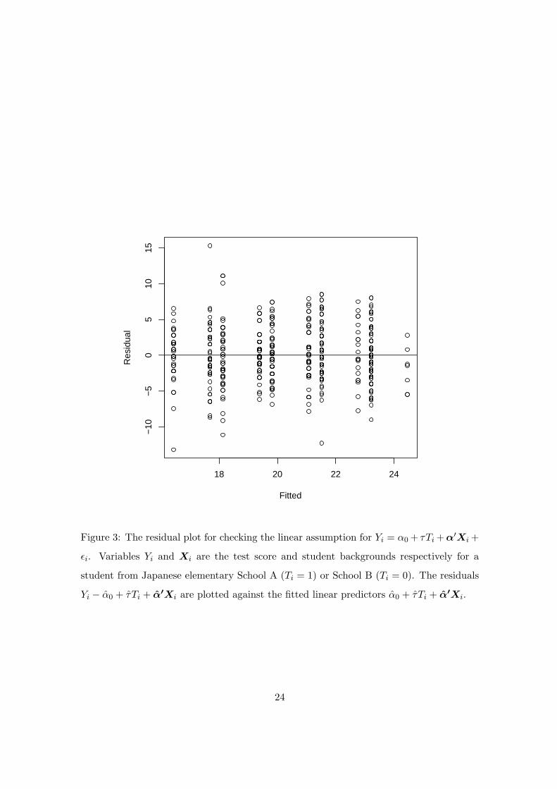
to the test scores from the students. First, we check Assumptions I and II simultaneously.

Assumptions I and II imply the relations

Yi = Yi(0) + τTi,

Yi(0) = α0 + α′Xi + εi,

for all i. Here the error term εi has zero mean. Combining the preceding pair of displayed

equations, we have

Yi = α0 + τTi + α′Xi + εi. (19)

The linearity assumption in (19) can be checked by the residual plot, a popular tool for

regression analyses. The residual plot displayed in Figure 3 shows no systematic departure

from the linear assumption. Next, we check Assumption III. Note that Assumption III is

equivalent to the normality assumption for εi under the linear model. We display the Q-Q

17

plot in Figure 4 to check the normality of the residuals. The plot forms a approximately

straight line except a few outlying observations in the tails. In general, we find no evidence

for rejecting Assumptions I-III.

Now we test the assumption H0 using the likelihood ratio test based on Assumptions

I-III. The likelihood ratio statistic for this data set is 2(l̂1 − l̂0) = 0.00094 and the cor-

responding p-value is 0.976. We do not find a statistical evidence for the departure from

H0. Assuming the strong ignorability, the X-adjusted nonparametric estimator in (1) pro-

vides a valid point estimates for the program effect τ̂ = 1.525 with 95% confidence interval

(0.713,2.597). The interval is away from zero, and it provide the significant evidence for

the positive educational effect for School A. Alternatively, it is possible to estimate the

treatment effect using the maximized likelihood methods. We obtain estimates τ̂0 = 1.760

under H0 : γ = 0 and τ̂1 = 1.895 under H0 ∪ H1 respectively. Note that the distance

between τ̂ and τ̂0 are close to each other. The difference between the nonparametric and

model-based estimates is expected to be small when the model is valid (White 1981).

In addition to the p-value from the likelihood ratio statistics, the small difference sug-

gests that the assumed normal disbribution model with the strong ignorability is a good

approximation for the data set

6 CONCLUSION

In this paper, we have proposed a hypothesis test for assessing the assumption of strong

ignorability. The logic of non-identifiability dilemma revealed that the assumption of

strong ignorability is not testable without appropriate distributional assumptions. By

imposing appropriate parametric assumptions (Assumptions I-III and logistic model) on

the counterfactual models, we have shown that the strong ignorability can be empirically

checked by the likelihood ratio test. Permitting flexible parametric families based on the

GLM, we have emphasized that the likelihood ratio test is very general and applicable to

many different types of data. We have derived a simple algorithm when the counterfac-

tual models follows a normal distribution. Also, extension for multivariate counterfactual

18

models is briefly discussed. Simulation studies indicate that the proposed test has regular

power properties if the Assumptons I-III are true. On the other hand, if the parametric

assumption is wrong, the test can fail to provide correct type I error rates.

To identify the assumption of strong ignorability, Assumption I (additive treatment

effect model) plays a key role in the likelihood construction. However, it is not clear that

Assumption I is valid in many application studies, though it is easy to generate such types

of data in simulations. Although some empirical procedures for checking Assumption I

and II simultaneously is provided in Section 5, we do not develop a saisfactory method

for checking Assumption I. There is a need for further research on the applicability of

Assumption I in real data.

We showed how the assumption of strong ignorability can be empirically assessed under

the GLM type framework with a simple example for the normal distribution case. The

development of algorithms for the other types of models, such as exponential, gamma

and Poisson-type distribution is mandated before the proposed method can be used more

generally. We leave this as a topic for further investigation.

Researchers may perform the likelihood ratio test to check H0 before making a statis-

tical inference on the treatment effect. If the test reject H0, the data may indicate either

the violation of the strong ignorability, or perhaps wrong distributional assumptions in

Assumptions I-III. The small p-value of the test results may give us insight on the mecha-

nism of the treatment assignment that may deserve further investigation. Specifically, the

existence of unobserved confounding variables may be suspected for such a case.

Finally, we note that the proposed method and sensitivity analysis play different roles

in the assessment for the assumption of strong ignorability. The porposed test checks the

validity of the assumption of strong ignorability while the sensitivity analysis investigates

the robustness of the treatment effect under the violation from the strong ignorability.

Combined use of these techniquues may enhance the integrity of a statistical inference for

the average treatment effect from observational data.

19

References

[1] Cochran, W. G. (1965), “The Planning of Observational Studies of Human Population

(with discussion),” Journal of the Royal Statistical Society, Series B, 128, 234-235.

[2] Coleman, J. S., Hoffer, T., Kilgore, S. (1982), High School Achievement, New York:

Basic.

[3] Dawid, A. P. (1979), “Conditional Independence in Statistical Theory,” Journal of

the Royal Statistical Society, Series B, 41, 1-31.

[4] Dehejia, R. H., and Wahba, S. (1998), “Causal Effects in Nonexperimental Stud-

ies: Reevaluating the Evaluation of Training Programs,” Journal of the American

Statistical Association, 94, 1053-1062.

[5] Goldberger, A. S. and Cain, G. G. (1982), “The Causal Analysis of Cognitive Out-

comes in the Coleman, Hoffer and Kilgore Report,” Sociology of Education, 55, 103-

122.

[6] Heckman, J., Ichimura, H., Smith, J. and Todd, P. (1998), “Characterizing Selection

Bias Using Experimental Data,” Econometrica, 66, 1017-1098.

[7] Hodges, J. and Lehmann, E. (1963), “Estimates of Location Based on Rank Tests,”

Annals of Mathematical Statistics, 34, 598-611.

[8] Hong, G. and Raudenbush, S. W. (2006), “Evaluating Kindergarten Retention Policy:

A Case Study of Causal Inference for Multilevel Observational Data,” Journal of the

American Statistical Association, 101, 901-910.

[9] Katsuyama, H., Nishigaki, C. and Wang, J. (2006), “A Study on the Effect of English

Teaching in Public Elementary Schools,” KATE Bulletin, 20, 113-124.

[10] Klein, J. P. and Moeschberger, M. L. (2003), Survival Analysis: Techniques for Cen-

sored and Truncated Data, New York: Springer.

20

[11] Lange K. L., Little, R. J. A. and Taylor, J. M. G (1989), “Robust Statistical Modeling

Using the t-Distribution,” Journal of the American Statistical Association, 84, 881-

896.

[12] Lehmann, E. L. (1975), Nonparametrics: Statistical Methods Based on Ranks, San

Francisco: Holden-Day.

[13] McCullagh, N. T. and Nelder, J. A. (1991), Generalized Linear Models, 2nd ed.,

London: Chapman & Hall/CRC.

[14] Morgan, S. L. (2001), “Counterfactuals, Causal Effect Heterogeneity, and the Catholic

School Effect on Learning,” Sociology of Education, 74, 341-374.

[15] Pearl, J. (2001), “Causal Inference in the Health Sciences: A Conceptual Introduc-

tion,” Health Services and Outcomes Research Methodology, 2, 189-220.

[16] Rosenbaum, P. (1984), “From Association to Causation in Observational Studies:

The Role of Strongly Ignorable Treatment Assignment,” Journal of the American

Statistical Association, 79, 41-48.

[17] Rosenbaum, P. (2002), Observational Studies, New York: Springer-Verlag.

[18] Rosenbaum, P. and Rubin, D. (1983), “The Central Role of the Propensity Score in

Observational Studies for Causal Effects,” Biometrika, 70, 41-55.

[19] Van Der Vaart, A. W. (1998), Asymptotic Statistics, Cambridge: Cambridge Univer-

sity Press.

[20] White, H. (1981), “Consequences and Detection of Misspecified Nonlinear Regression

Models,” Journal of the American Statistical Association, 76, 1065-1073.

[21] Winship, C. and Morgan, S. L. (1999), “The Estimation of Causal Effects from Ob-

servational Data,” Annual Review of Sociology, 25, 659-706.

21

−3 −2 −1 0 1 2 3

020

4060

8010

0

α = (1, 1)

γ

Pow

er(%

)

n=200

n=400

n=600

5%line

−3 −2 −1 0 1 2 3

020

4060

8010

0

α = (1, − 1)

γ

Pow

er(%

) n=200

n=400n=600

5%line

−3 −2 −1 0 1 2 3

020

4060

8010

0

α = (− 1, 1)

γ

Pow

er(%

)

n=200

n=400n=600

5%line

−3 −2 −1 0 1 2 3

020

4060

8010

0

α = (− 1, − 1)

γ

Pow

er(%

) n=200

n=400n=600

5%line

Figure 1: Power curves for sample sizes n = 200 (Solid Line), n = 400 (Dashed Line) and

n = 600 (Dashed and Dotted Line) based on 1000 replicates. Potential outcomes Y (0)

are generated from the normal distributions with mean 1 + α′X and variance 1. The

assignment variable T follows a Bernoulli random variable with the probability p modeled

by the logit model logit(p) = −1 + X1 + X2.

22

0.0 0.5 1.0 1.5

010

2030

4050

60

α = (1, 1)

Kurtosis

Typ

e I e

rror

(%)

n=200

n=400

n=600

5%line

0.0 0.5 1.0 1.5

010

2030

4050

60

α = (1, − 1)

Kurtosis

Typ

e I e

rror

(%)

n=200

n=400

n=600

5%line

0.0 0.5 1.0 1.5

010

2030

4050

60

α = (− 1, 1)

Kurtosis

Typ

e I e

rror

(%)

n=200

n=400

n=600

5%line

0.0 0.5 1.0 1.5

010

2030

4050

60

α = (− 1, 1)

Kurtosis

Typ

e I e

rror

(%)

n=200

n=400

n=600

5%line

Figure 2: Type I error rates for sample sizes n = 200 (Solid Line), n = 400 (Dashed Line)

and n = 600 (Dashed and Dotted Line) based on 1000 replicates. Potential outcomes Y (0)

are generated from the misspecified t-distributions with mean 1 + α′X, scale parameter

1 and the kurtosis ν ∈ [0, 1.5]. The assignment variable T follows a Bernoulli distribution

with the probability p modeled by the logit model logit(p) = −1 + X1 + X2.

23

18 20 22 24

−10

−5

05

1015

Fitted

Res

idua

l

Figure 3: The residual plot for checking the linear assumption for Yi = α0 + τTi +α′Xi +

εi. Variables Yi and Xi are the test score and student backgrounds respectively for a

student from Japanese elementary School A (Ti = 1) or School B (Ti = 0). The residuals

Yi − α̂0 + τ̂Ti + α̂0Xi are plotted against the fitted linear predictors α̂0 + τ̂Ti + α̂0Xi.

24

−3 −2 −1 0 1 2 3

−10

−5

05

1015

Theoretical Quantiles

Sam

ple

Qua

ntile

s

Figure 4: Q-Q plot for checking the normality assumption for the error distribution in

Yi = α0 +τTi +α′Xi + εi. Variables Yi and Xi are the test score and student backgrounds

respectively for a student from Japanese elementary School A (Ti = 1) or School B (Ti =

0). The straight line passes through the first and third quartiles.

25