Section 4 Matching Estimator

Matching Estimators

• Key Idea: The matching method compares the outcomes of program participants with those of matchednonparticipants, where matches are chosen on the basis of similarity in observed characteristics.

• Main advantage of matching estimators: they typically do not require specifying a functional form of the outcome equation and are therefore not susceptible to misspecification bias along that dimension.

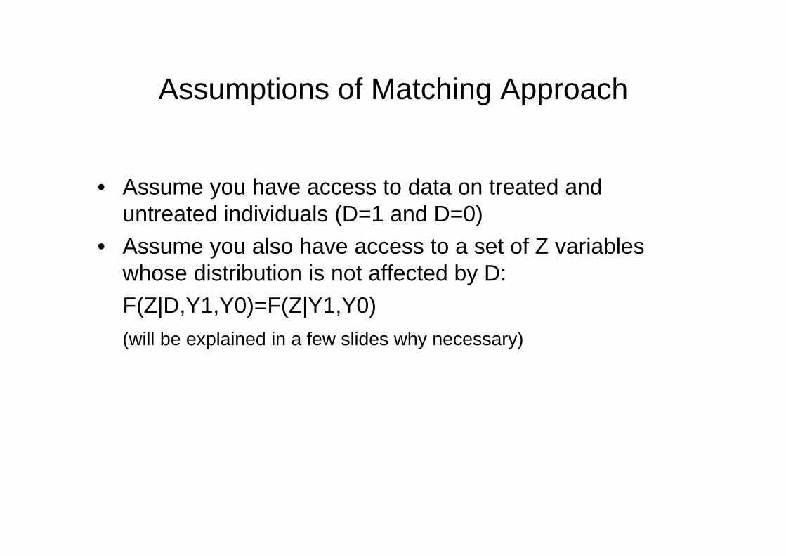
Assumptions of Matching Approach

• Assume you have access to data on treated and untreated individuals (D=1 and D=0)

• Assume you also have access to a set of Z variables whose distribution is not affected by D:F(Z|D,Y1,Y0)=F(Z|Y1,Y0) (will be explained in a few slides why necessary)

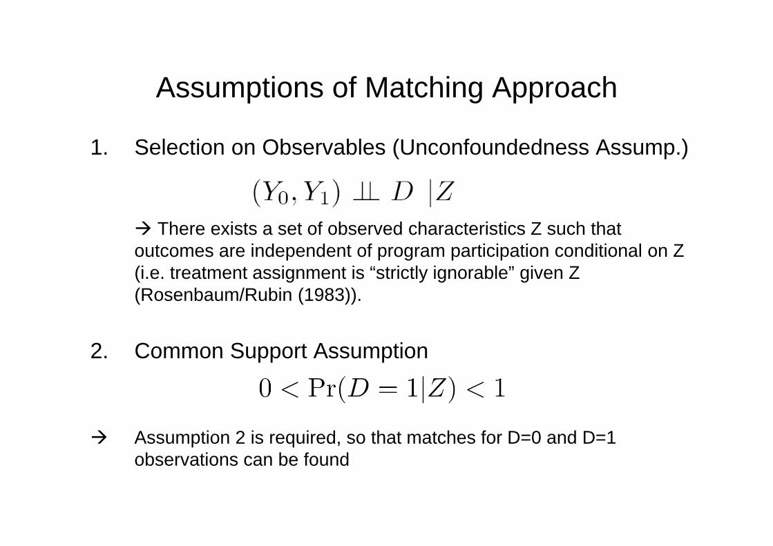
Assumptions of Matching Approach

1. Selection on Observables (Unconfoundedness Assump.)

There exists a set of observed characteristics Z such that outcomes are independent of program participation conditional on Z (i.e. treatment assignment is “strictly ignorable” given Z (Rosenbaum/Rubin (1983)).

2. Common Support Assumption

Assumption 2 is required, so that matches for D=0 and D=1 observations can be found

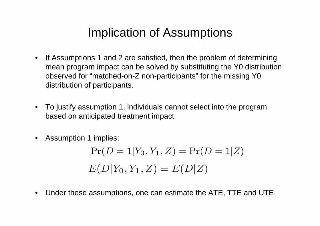
Implication of Assumptions

• If Assumptions 1 and 2 are satisfied, then the problem of determining mean program impact can be solved by substituting the Y0 distribution observed for “matched-on-Z non-participants” for the missing Y0 distribution of participants.

• To justify assumption 1, individuals cannot select into the program based on anticipated treatment impact

• Assumption 1 implies:

• Under these assumptions, one can estimate the ATE, TTE and UTE

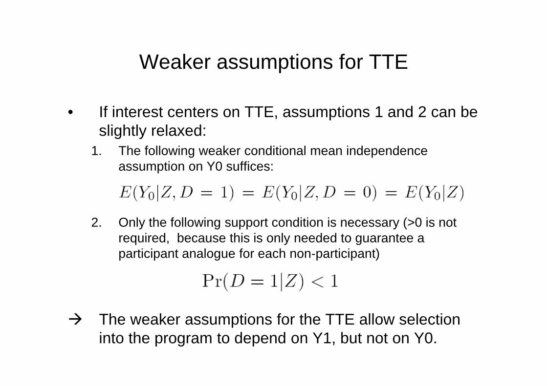
Weaker assumptions for TTE

• If interest centers on TTE, assumptions 1 and 2 can be slightly relaxed:

1. The following weaker conditional mean independence assumption on Y0 suffices:

2. Only the following support condition is necessary (>0 is not required, because this is only needed to guarantee a participant analogue for each non-participant)

The weaker assumptions for the TTE allow selection into the program to depend on Y1, but not on Y0.

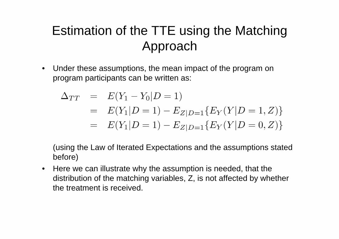
Estimation of the TTE using the Matching Approach

• Under these assumptions, the mean impact of the program on program participants can be written as:

(using the Law of Iterated Expectations and the assumptions stated before)

• Here we can illustrate why the assumption is needed, that the distribution of the matching variables, Z, is not affected by whether the treatment is received.

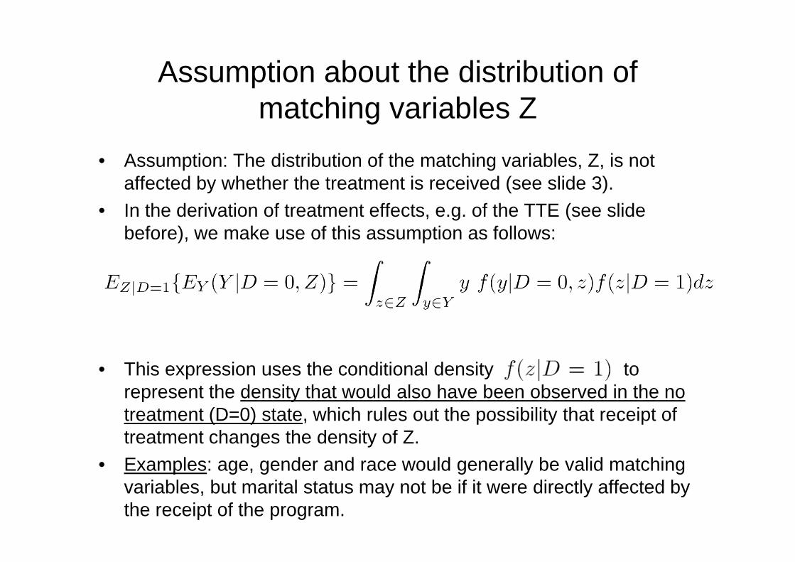
Assumption about the distribution of matching variables Z

• Assumption: The distribution of the matching variables, Z, is not affected by whether the treatment is received (see slide 3).

• In the derivation of treatment effects, e.g. of the TTE (see slide before), we make use of this assumption as follows:

• This expression uses the conditional density to represent the density that would also have been observed in the no treatment (D=0) state, which rules out the possibility that receipt of treatment changes the density of Z.

• Examples: age, gender and race would generally be valid matching variables, but marital status may not be if it were directly affected by the receipt of the program.

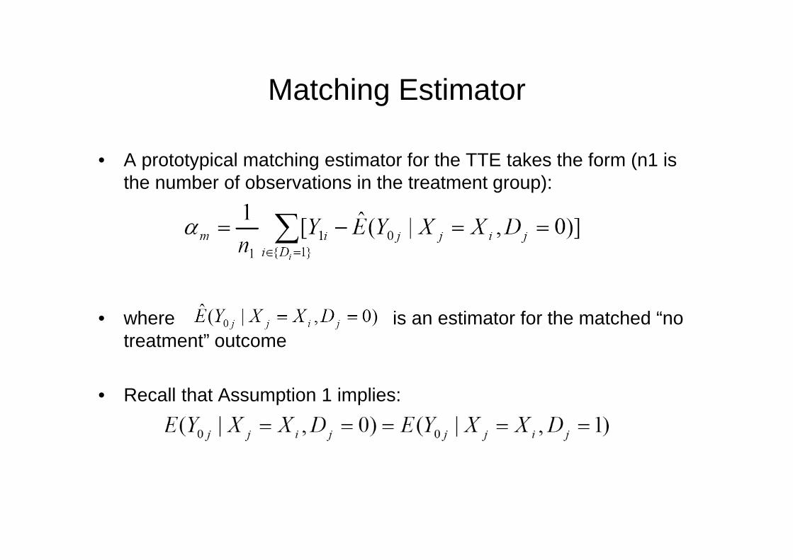
Matching Estimator

• A prototypical matching estimator for the TTE takes the form (n1 is the number of observations in the treatment group):

• where is an estimator for the matched “no treatment” outcome

• Recall that Assumption 1 implies:

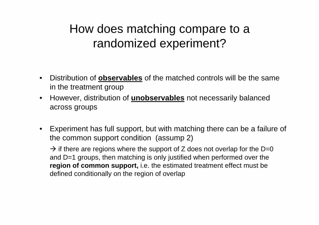
How does matching compare to a randomized experiment?

• Distribution of observables of the matched controls will be the same in the treatment group

• However, distribution of unobservables not necessarily balanced across groups

• Experiment has full support, but with matching there can be a failure of the common support condition (assump 2) if there are regions where the support of Z does not overlap for the D=0 and D=1 groups, then matching is only justified when performed over the region of common support, i.e. the estimated treatment effect must be defined conditionally on the region of overlap

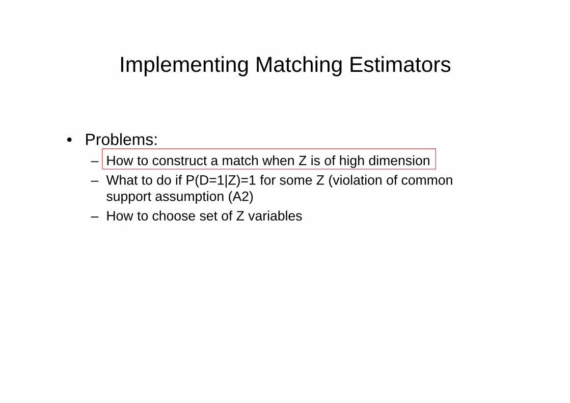
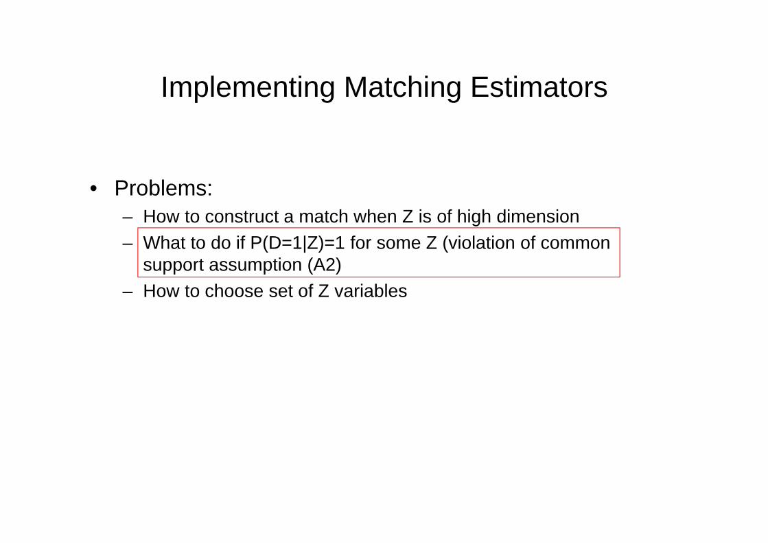
Implementing Matching Estimators

• Problems:– How to construct a match when Z is of high dimension– What to do if P(D=1|Z)=1 for some Z (violation of common

support assumption (A2)– How to choose set of Z variables

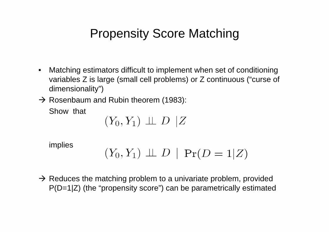
Propensity Score Matching

• Matching estimators difficult to implement when set of conditioning variables Z is large (small cell problems) or Z continuous (“curse of dimensionality”)

Rosenbaum and Rubin theorem (1983):Show that

implies

Reduces the matching problem to a univariate problem, provided P(D=1|Z) (the “propensity score”) can be parametrically estimated

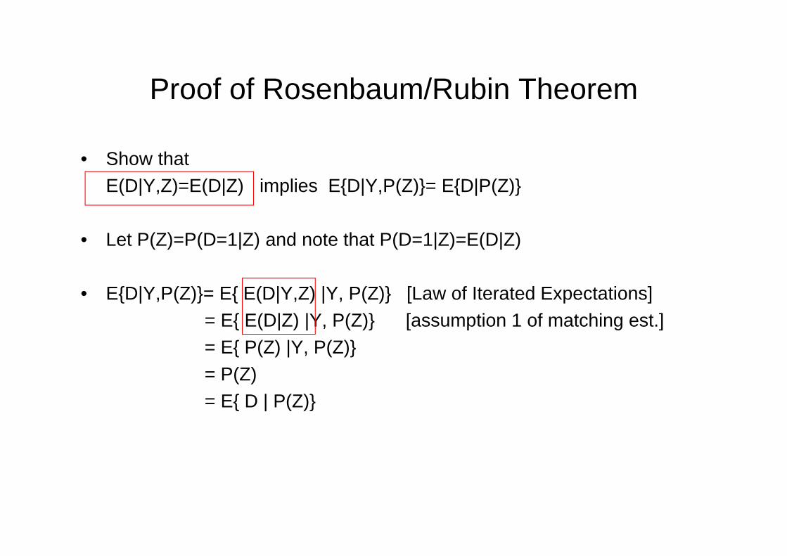
Proof of Rosenbaum/Rubin Theorem

• Show thatE(D|Y,Z)=E(D|Z) implies E{D|Y,P(Z)}= E{D|P(Z)}

• Let P(Z)=P(D=1|Z) and note that P(D=1|Z)=E(D|Z)

• E{D|Y,P(Z)}= E{ E(D|Y,Z) |Y, P(Z)} [Law of Iterated Expectations]= E{ E(D|Z) |Y, P(Z)} [assumption 1 of matching est.]= E{ P(Z) |Y, P(Z)}= P(Z)= E{ D | P(Z)}

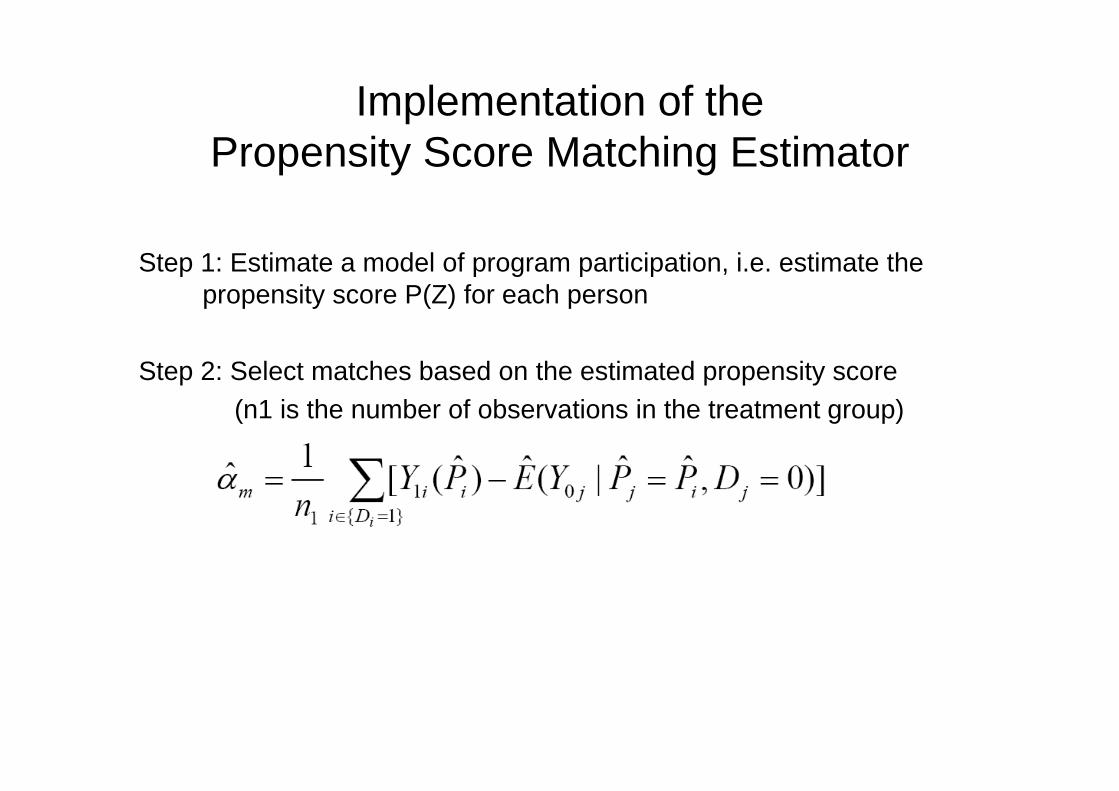
Implementation of the Propensity Score Matching Estimator

Step 1: Estimate a model of program participation, i.e. estimate the propensity score P(Z) for each person

Step 2: Select matches based on the estimated propensity score (n1 is the number of observations in the treatment group)

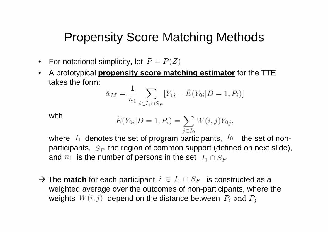
Propensity Score Matching Methods

• For notational simplicity, let P=P(Z)• A prototypical propensity score matching estimator for the TTE

takes the form:

with

where denotes the set of program participants, the set of non-participants, the region of common support (defined on next slide), and is the number of persons in the set

The match for each participant is constructed as a weighted average over the outcomes of non-participants, where the weights depend on the distance between

Implementing Matching Estimators

• Problems:– How to construct a match when Z is of high dimension– What to do if P(D=1|Z)=1 for some Z (violation of common

support assumption (A2)– How to choose set of Z variables

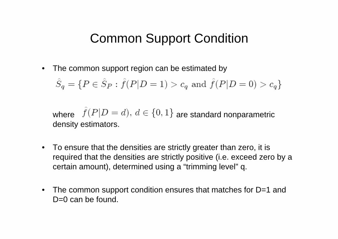
Common Support Condition

• The common support region can be estimated by

where are standard nonparametric density estimators.

• To ensure that the densities are strictly greater than zero, it is required that the densities are strictly positive (i.e. exceed zero by a certain amount), determined using a “trimming level” q.

• The common support condition ensures that matches for D=1 and D=0 can be found.

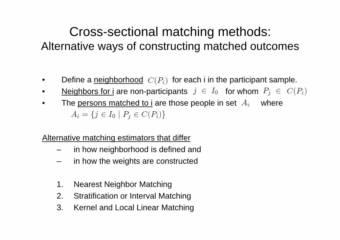
Cross-sectional matching methods: Alternative ways of constructing matched outcomes

• Define a neighborhood for each i in the participant sample.• Neighbors for i are non-participants for whom• The persons matched to i are those people in set where

Alternative matching estimators that differ – in how neighborhood is defined and – in how the weights are constructed

1. Nearest Neighbor Matching2. Stratification or Interval Matching3. Kernel and Local Linear Matching

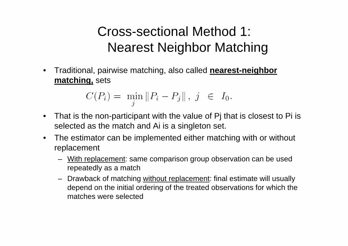
Cross-sectional Method 1:Nearest Neighbor Matching

• Traditional, pairwise matching, also called nearest-neighbor matching, sets

• That is the non-participant with the value of Pj that is closest to Pi is selected as the match and Ai is a singleton set.

• The estimator can be implemented either matching with or without replacement– With replacement: same comparison group observation can be used

repeatedly as a match– Drawback of matching without replacement: final estimate will usually

depend on the initial ordering of the treated observations for which the matches were selected

Cross-sectional Method 1:Nearest Neighbor Matching

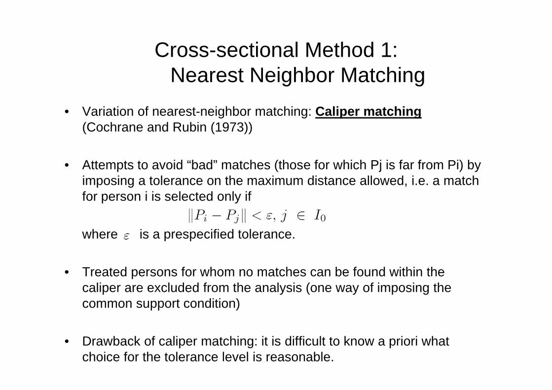
• Variation of nearest-neighbor matching: Caliper matching(Cochrane and Rubin (1973))

• Attempts to avoid “bad” matches (those for which Pj is far from Pi) by imposing a tolerance on the maximum distance allowed, i.e. a match for person i is selected only if

where is a prespecified tolerance.

• Treated persons for whom no matches can be found within the caliper are excluded from the analysis (one way of imposing the common support condition)

• Drawback of caliper matching: it is difficult to know a priori what choice for the tolerance level is reasonable.

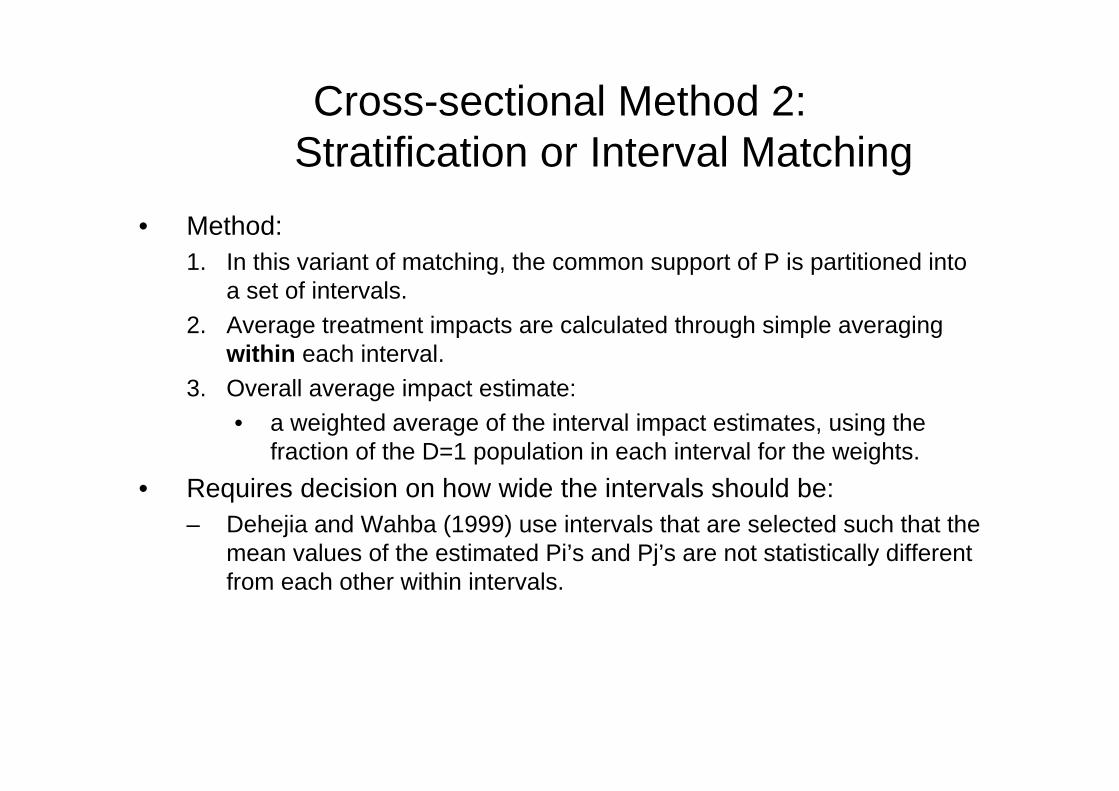
Cross-sectional Method 2:Stratification or Interval Matching

• Method:1. In this variant of matching, the common support of P is partitioned into

a set of intervals.2. Average treatment impacts are calculated through simple averaging

within each interval.3. Overall average impact estimate:

• a weighted average of the interval impact estimates, using the fraction of the D=1 population in each interval for the weights.

• Requires decision on how wide the intervals should be:– Dehejia and Wahba (1999) use intervals that are selected such that the

mean values of the estimated Pi’s and Pj’s are not statistically different from each other within intervals.

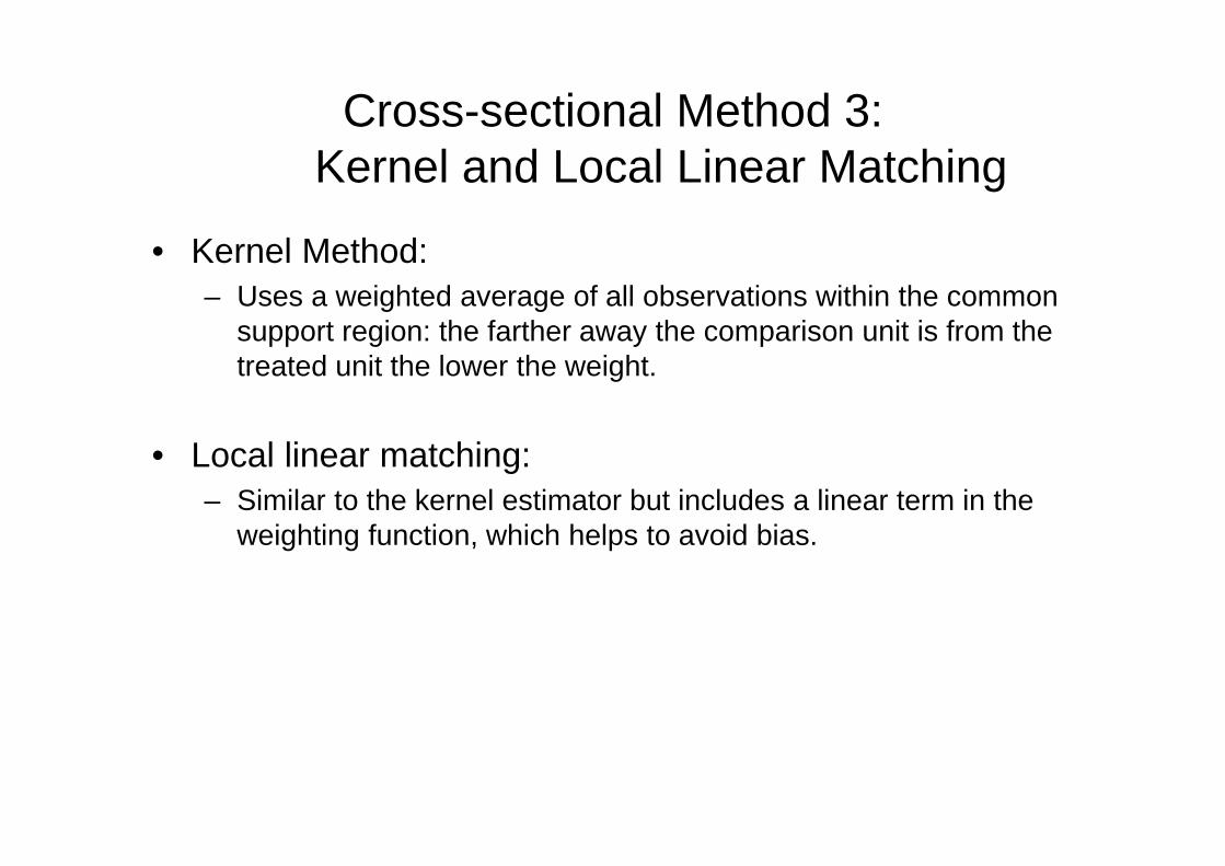
Cross-sectional Method 3:Kernel and Local Linear Matching

• Kernel Method:– Uses a weighted average of all observations within the common

support region: the farther away the comparison unit is from the treated unit the lower the weight.

• Local linear matching:– Similar to the kernel estimator but includes a linear term in the

weighting function, which helps to avoid bias.

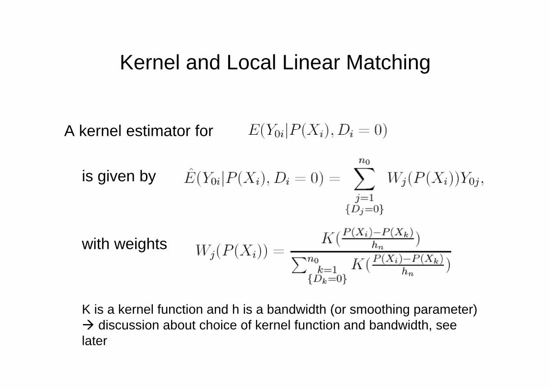
Kernel and Local Linear Matching

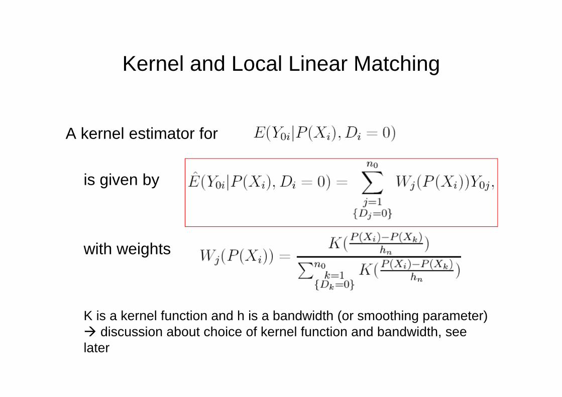
A kernel estimator for

is given by

with weights

K is a kernel function and h is a bandwidth (or smoothing parameter) discussion about choice of kernel function and bandwidth, see later

Intro to Nonparametric Estimation

• Reference: Angus Deaton “The Analysis of Household Surveys” TO READ– ch. 3.2 Nonparametric methods for estimating density functions

(p. 169-175), Nonparametric regression analysis (p. 191-199)

• Kernel density estimation• Kernel regression• Choice of kernel and choice of bandwidth (trade-off

between bias and variance)• Local linear estimation: when and why better?

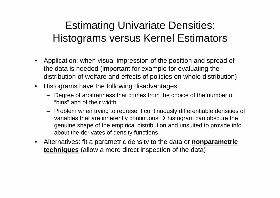
Estimating Univariate Densities: Histograms versus Kernel Estimators

• Application: when visual impression of the position and spread of the data is needed (important for example for evaluating the distribution of welfare and effects of policies on whole distribution)

• Histograms have the following disadvantages: – Degree of arbitrariness that comes from the choice of the number of

“bins” and of their width– Problem when trying to represent continuously differentiable densities of

variables that are inherently continuous histogram can obscure the genuine shape of the empirical distribution and unsuited to provide info about the derivates of density functions

• Alternatives: fit a parametric density to the data or nonparametric techniques (allow a more direct inspection of the data)

Nonparametric density estimation

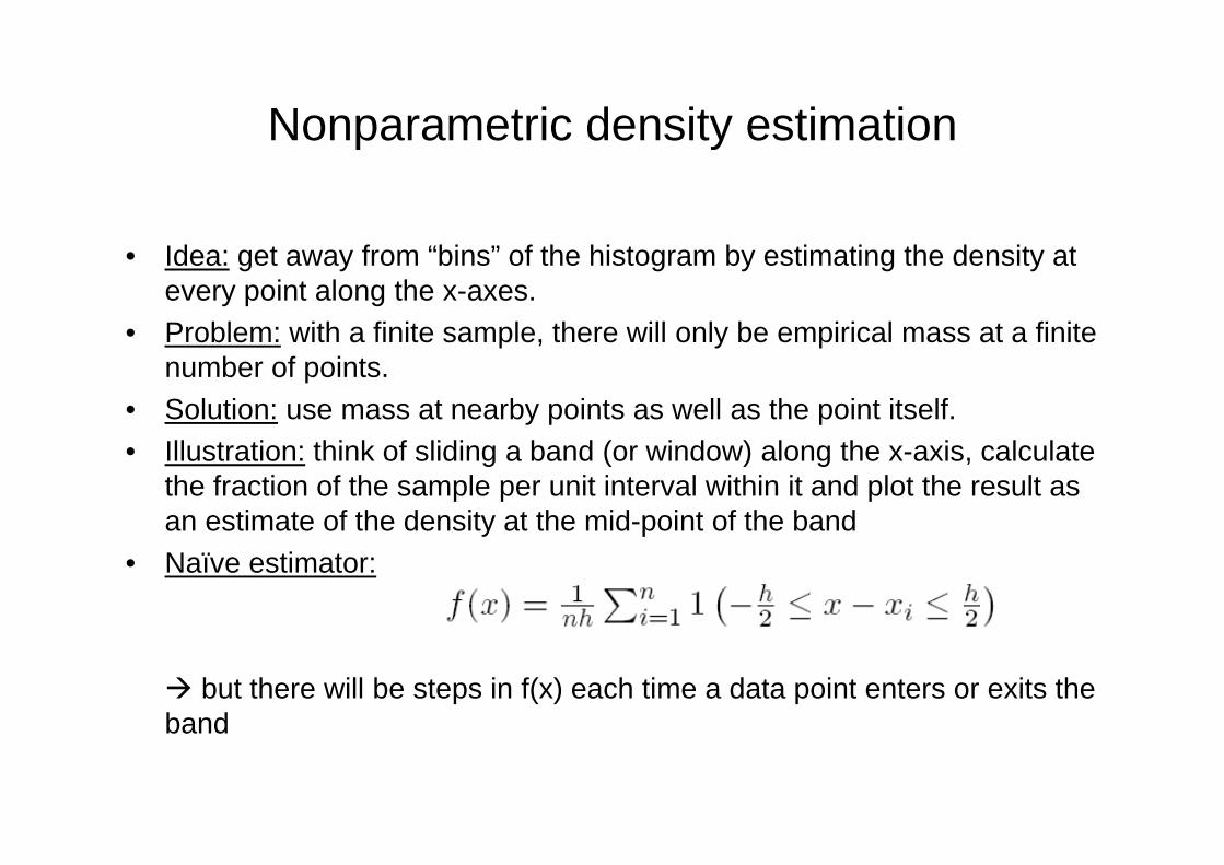
• Idea: get away from “bins” of the histogram by estimating the density at every point along the x-axes.

• Problem: with a finite sample, there will only be empirical mass at a finite number of points.

• Solution: use mass at nearby points as well as the point itself.• Illustration: think of sliding a band (or window) along the x-axis, calculate

the fraction of the sample per unit interval within it and plot the result as an estimate of the density at the mid-point of the band

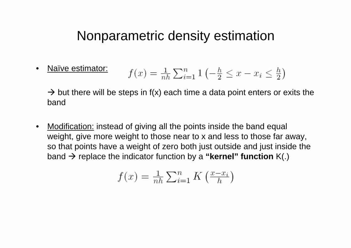
• Naïve estimator:

but there will be steps in f(x) each time a data point enters or exits the band

Nonparametric density estimation

• Naïve estimator:

but there will be steps in f(x) each time a data point enters or exits the band

• Modification: instead of giving all the points inside the band equal weight, give more weight to those near to x and less to those far away, so that points have a weight of zero both just outside and just inside the band replace the indicator function by a “kernel” function K(.)

Choice of Kernel and Bandwidth

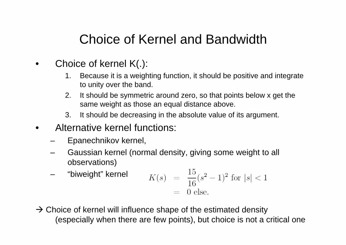
• Choice of kernel K(.): 1. Because it is a weighting function, it should be positive and integrate

to unity over the band.2. It should be symmetric around zero, so that points below x get the

same weight as those an equal distance above.3. It should be decreasing in the absolute value of its argument.

• Alternative kernel functions:– Epanechnikov kernel, – Gaussian kernel (normal density, giving some weight to all

observations) – “biweight” kernel

Choice of kernel will influence shape of the estimated density (especially when there are few points), but choice is not a critical one

Choice of Kernel and Bandwidth

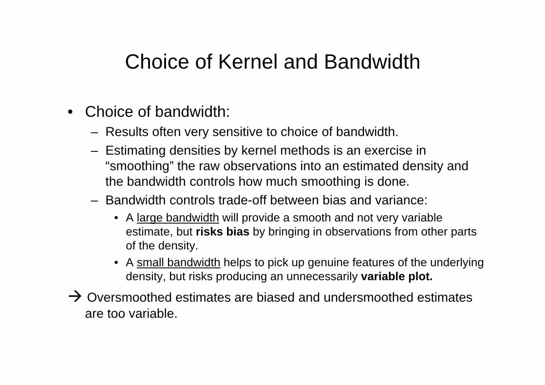
• Choice of bandwidth:– Results often very sensitive to choice of bandwidth.– Estimating densities by kernel methods is an exercise in

“smoothing” the raw observations into an estimated density and the bandwidth controls how much smoothing is done.

– Bandwidth controls trade-off between bias and variance:• A large bandwidth will provide a smooth and not very variable

estimate, but risks bias by bringing in observations from other parts of the density.

• A small bandwidth helps to pick up genuine features of the underlying density, but risks producing an unnecessarily variable plot.

Oversmoothed estimates are biased and undersmoothed estimates are too variable.

Choice of Kernel and Bandwidth

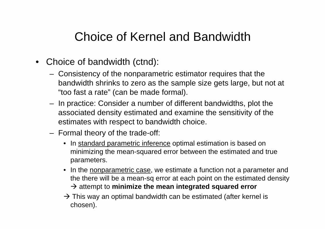
• Choice of bandwidth (ctnd):– Consistency of the nonparametric estimator requires that the

bandwidth shrinks to zero as the sample size gets large, but not at “too fast a rate” (can be made formal).

– In practice: Consider a number of different bandwidths, plot the associated density estimated and examine the sensitivity of the estimates with respect to bandwidth choice.

– Formal theory of the trade-off:• In standard parametric inference optimal estimation is based on

minimizing the mean-squared error between the estimated and true parameters.

• In the nonparametric case, we estimate a function not a parameter and the there will be a mean-sq error at each point on the estimated density attempt to minimize the mean integrated squared error

This way an optimal bandwidth can be estimated (after kernel is chosen).

Nonparametric Regression Analysis

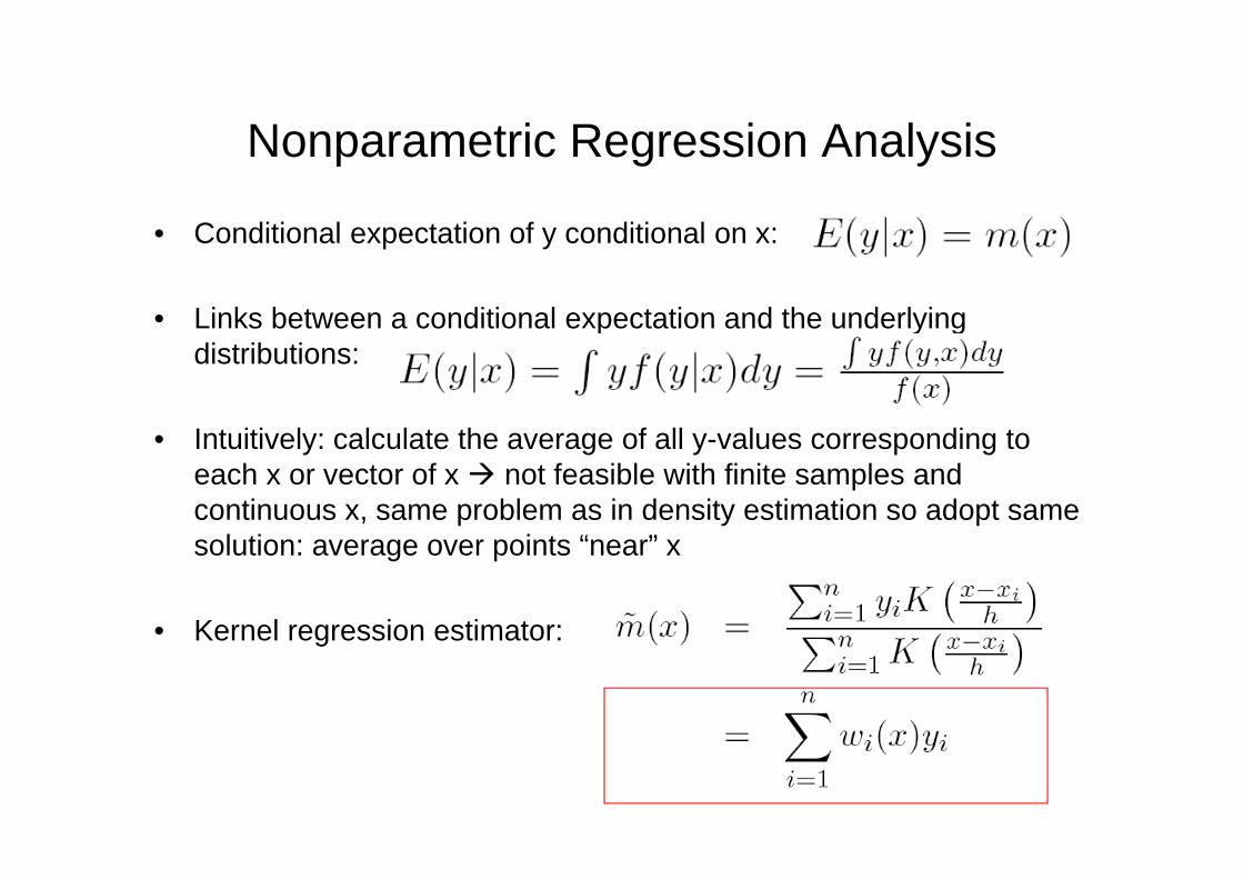
• Conditional expectation of y conditional on x:

• Links between a conditional expectation and the underlying distributions:

• Intuitively: calculate the average of all y-values corresponding to each x or vector of x not feasible with finite samples and continuous x, same problem as in density estimation so adopt same solution: average over points “near” x

• Kernel regression estimator:

Kernel and Local Linear Matching

A kernel estimator for

is given by

with weights

K is a kernel function and h is a bandwidth (or smoothing parameter) discussion about choice of kernel function and bandwidth, see later

Nonparametric Regression Analysis

• Important: it is not possible to calculate a conditional expectation for values of x where the density is zero in practice, problems whenever the estimated density is small or zero (will make the regression function imprecise)

• Main strength of nonparametric over parametric regression: assumes no functional form for the relationship, allowing the data to choose, not only parameter estimates, but the shape of the curve itself

• Weaknesses:– price of the flexibility is the much greater data requirements to

implementing nonparametric methods and the difficulties of handling high-dimensional problems (alternatives: polynomial regressions and semiparametric estimation)

– Nonparametric methods lack the menu of options that is available for parametric methods when dealing with simultaneity, measurement error, selectivity and so forth

Locally Linear Regression

• Read Angus Deaton “The Analysis of Household Surveys” (p. 197-199)

important: will be used again later on

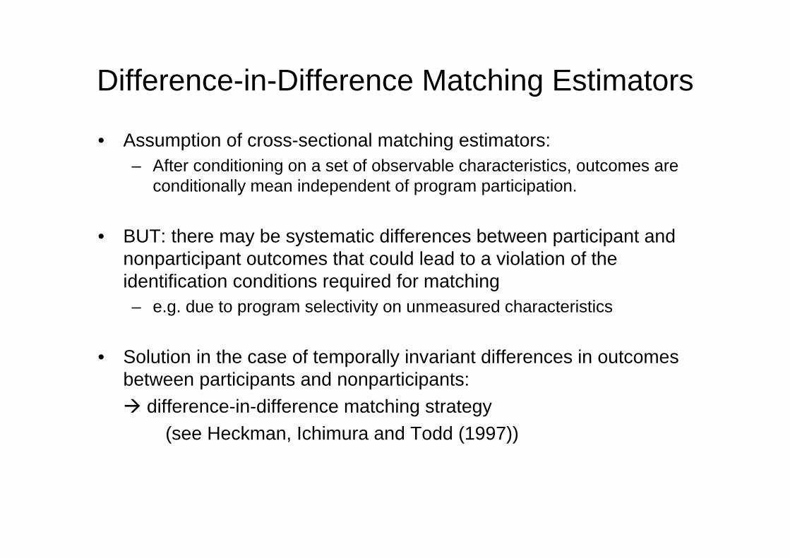
Difference-in-Difference Matching Estimators

• Assumption of cross-sectional matching estimators:– After conditioning on a set of observable characteristics, outcomes are

conditionally mean independent of program participation.

• BUT: there may be systematic differences between participant and nonparticipant outcomes that could lead to a violation of the identification conditions required for matching– e.g. due to program selectivity on unmeasured characteristics

• Solution in the case of temporally invariant differences in outcomes between participants and nonparticipants: difference-in-difference matching strategy

(see Heckman, Ichimura and Todd (1997))

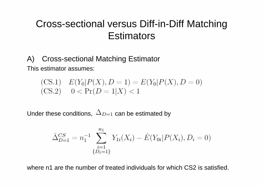
Cross-sectional versus Diff-in-Diff Matching Estimators

A) Cross-sectional Matching EstimatorThis estimator assumes:

Under these conditions, can be estimated by

where n1 are the number of treated individuals for which CS2 is satisfied.

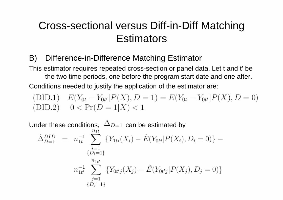
Cross-sectional versus Diff-in-Diff Matching Estimators

B) Difference-in-Difference Matching EstimatorThis estimator requires repeated cross-section or panel data. Let t and t’ be

the two time periods, one before the program start date and one after.Conditions needed to justify the application of the estimator are:

Under these conditions, can be estimated by

Assessing the Variability of Matching Estimators

• Distribution theory for cross-sectional and DID kernel and local linear matching estimators: see Heckman, Ichimura and Todd (1998)

• But implementing the asymptotic standard error formulae can be cumbersome, so standard errors for matching estimators are often generated using bootstrap resampling methods

• This is valid for kernel or local linear matching estimators, but not for nearest neighbor matching estimators (see Abadie and Imbens (2004), also for alternatives in that case)