put–call parity and market frictions -...
TRANSCRIPT

Available online at www.sciencedirect.com
ScienceDirect
Journal of Economic Theory 157 (2015) 730–762
www.elsevier.com/locate/jet
Put–Call Parity and market frictions ✩
S. Cerreia-Vioglio, F. Maccheroni, M. Marinacci ∗
Università Bocconi and IGIER, Italy
Received 6 November 2013; final version received 5 September 2014; accepted 16 December 2014
Available online 6 January 2015
Abstract
We extend the Fundamental Theorem of Finance and the Pricing Rule Representation Theorem to the case in which market frictions are taken into account but the Put–Call Parity is still assumed to hold. In turn, we obtain a representation of the pricing rule as a discounted expectation with respect to a nonadditive risk neutral probability.© 2014 Elsevier Inc. All rights reserved.
JEL classification: G12; G13; D81
Keywords: Put–Call Parity; Market frictions; Fundamental Theorem of Finance; No arbitrage; Choquet pricing
1. Introduction
We extend the Fundamental Theorem of Finance and the Pricing Rule Representation The-orem to markets with frictions.1 We assume the Put–Call Parity and the absence of arbitrage opportunities and, under these hypotheses, we obtain a representation of the pricing rule as a discounted expectation with respect to a nonadditive risk neutral probability. In other words,
✩ We thank Alain Chateauneuf and Paolo Guasoni for very useful discussions and comments. Simone Cerreia-Vioglio and Fabio Maccheroni gratefully acknowledge the financial support of MIUR (PRIN grant 20103S5RN3_005) and of the AXA Research Fund. Massimo Marinacci gratefully acknowledges the financial support of the European Research Council (advanced grant BRSCDP-TEA) and of the AXA Research Fund.
* Corresponding author at: U. Bocconi, via Sarfatti 25, 20136, Milano, Italy.E-mail address: [email protected] (M. Marinacci).
1 The combination of these two results is also known in the literature as the Fundamental Theorem of Asset Pricing (see, e.g., [16,12]).
http://dx.doi.org/10.1016/j.jet.2014.12.0110022-0531/© 2014 Elsevier Inc. All rights reserved.

S. Cerreia-Vioglio et al. / Journal of Economic Theory 157 (2015) 730–762 731
the market prices contingent claims as an ambiguity sensitive, but risk neutral, decision maker. As a further contribution, we remove the state space structure and the contingent claim repre-sentation that are usually assumed exogenously to model assets and markets. In particular, this allows us to provide a unique mathematical framework where we can both discuss the Funda-mental Theorem of Finance and the Pricing Rule Representation Theorem.
Most of the fundamental theory of asset pricing relies on two main hypotheses: frictionless markets and absence of arbitrage.2 On the other hand, frictions and transaction costs are present in financial markets and play an important role. Important evidence of these facts is the existence of bid–ask spreads (see, e.g., Amihud and Mendelson [3,4]). As a consequence, the Finance literature developed models that incorporate transaction costs and taxes (see, e.g., Garman and Ohlson [17], Prisman [35], Ross [39], Jouini and Kallal [26], and Luttmer [32]). In particular, [35,26,32] observe how taxes/transaction costs generate pricing rules that are not linear but still can be compatible with the no arbitrage assumption. Inter alia, Prisman [35] shows that convex transaction costs or taxes generate convex pricing rules. Furthermore, if transaction costs are different among securities but proportional to the volumes dealt, then the respective pricing rules are sublinear, as in [26,32].
Our approach is different. In a standard framework, the no friction assumption paired with the Law of One Price yields the fundamental Put–Call Parity, first discovered by Stoll [44] (see also Kruizenga [30]). Moreover, the no friction assumption also implies that when a risk-free position is added to an existing portfolio the price of the resulting portfolio is equal to the price of the original portfolio plus the price of the position on the risk-free asset. This last implication is basi-cally equivalent to say that the price on the market of the risk-free asset is linear and in particular the bid–ask spread is zero on this market. From an applied point of view, the absence of frictions on the market of the risk-free asset and the Put–Call Parity are two important assumptions since they can be empirically tested.3 These two joint properties are at the center of our study.
We study price functionals and pricing rules that satisfy a version of the Put–Call Parity and exhibit no frictions in the market of the risk-free asset. These two no frictions assumptions are conceptually much weaker than the standard one and much easier to test empirically. As in the standard case, we further retain a no arbitrage postulate. We show (Theorems 1 and 3) that these pricing rules can be characterized as discounted expectations with respect to a nonadditive prob-ability, that is, by using Choquet expectations. One important feature of our result is that Choquet pricing rules are characterized by preserving the aforementioned financial identities but, a pri-ori, they are not the direct result of assuming transaction costs, bid–ask spreads, or short-sales constraints. Instead, making these assumptions would naturally lead to sublinear pricing rules which have been studied exactly to account for transaction costs (as in Jouini and Kallal [26] and Luttmer [32]; see also Kabanov and Safarian [27]). It is then natural to ask what is the overlap between Choquet and sublinear pricing rules. Corollaries 1 and 2 show that a pricing rule is sub-linear and Choquet if and only if the nonadditive probability that represents it is concave. In this case, the set of consistent price systems coincides with the core of this nonadditive probability. Thus, among the others, we provide testable conditions under which transaction costs generate a sublinear pricing rule which is also a nonadditive expectation.
2 See, e.g., Ross [36,38], Cox and Ross [9], and, in a dynamic setting, Harrison and Kreps [23], Harrison and Pliska [24], and Delbaen and Schachermayer [11]. For an introduction to the topic, see Dybvig and Ross [14], Ross [40], Follmer and Schied [16], and Delbaen and Schachermayer [12].
3 The empirical validity of the Put–Call Parity condition should be tested by using European options data, like in Kamara and Miller [28], in order to avoid issues of early exercise.

732 S. Cerreia-Vioglio et al. / Journal of Economic Theory 157 (2015) 730–762
Subadditive Choquet pricing rules were first studied and characterized by Chateauneuf, Kast, and Lapied [8]. Theorem 1.1 of [8] offers a generalized version of the Representation Theorem for Choquet pricing rules. The main assumption in [8] is comonotonic additivity which is paired with an assumption of no arbitrage that we also use. Comonotonic additivity is, however, a diffi-cult property to test since it requires a contingent claim representation for the assets considered and it requires to verify the absence of frictions on a large class of assets’ pairs. On the other hand, our characterization of Choquet pricing relies on the Put–Call Parity (henceforth, also PCP) which is easier to test. In fact, in the literature there are several studies testing the validity of the PCP (see Stoll [44,45], Gould and Galai [20], Klemkosky and Resnick [29], and Kamara and Miller [28]).
Choquet Expected Utility (henceforth, CEU) was introduced in Economics to account for de-viations from the standard model of Subjective Expected Utility (henceforth, SEU) as formulated by Savage [41] and Anscombe and Aumann [5]. Schmeidler [43] (see also Gilboa [18]) shows instead how the CEU model can accommodate patterns of choice not consistent with the SEU model, like the ones contained in Ellsberg [15], while still being able to account for Ambigu-ity and Ambiguity Aversion.4 Despite sharing some of the mathematical tools coming from the literature of choice under Ambiguity, conceptually, the current paper is very different.
The rest of the paper is organized as follows. Section 2 contains our generalization of the Representation Theorem in the finite dimensional setting. We start in Section 2.1 with some mathematical preliminaries. In Section 2.2, we briefly review the famous Fundamental Theorem of Finance and the Pricing Rule Representation Theorem. Section 2.3 contains our main result: Theorem 1. In Section 2.4, we discuss some of its extensions. Appendix A provides the repre-sentation theorem on which our results hinge. Appendix B contains our main result in its most general form: Theorem 3. This result is stated and proved in a very general setting where we dispense with the assumptions of finite dimensionality and of existence of an underlying state space.
2. The finite dimensional case
2.1. Mathematical preliminaries
Consider a finite state space Ω = {ω1, . . . , ωm}.5 We endow Ω with the σ -algebra coinciding with the power set P(Ω). A nonadditive probability is a set function ν : P(Ω) → [0, 1] such that ν(∅) = 0, ν(Ω) = 1, and ν(A) ≤ ν(B) whenever A ⊆ B ⊆ Ω . We say that ν is a concave nonadditive probability if and only if for each A and B
ν(A ∩ B) + ν(A ∪ B) ≤ ν(A) + ν(B).
A probability μ is instead an additive set function such that μ(∅) = 0 and μ(Ω) = 1. Clearly, an additive probability can also be identified with a vector in Rm. A nonadditive probability ν is balanced if and only if there exists a probability μ such that μ ≤ ν. If a nonadditive probability is concave, then it is balanced, but the vice versa does not hold in general. Finally, we denote by core(ν) the set of all probabilities μ such that μ ≤ ν.
4 For a comprehensive recent survey on the literature of choice under Ambiguity, see Gilboa and Marinacci [19].5 In this section, we provide the mathematical preliminaries that are necessary for Section 2 and all the examples in the
paper which refer to this section. We refer the reader to Appendix A for all the other relevant mathematical notions.

S. Cerreia-Vioglio et al. / Journal of Economic Theory 157 (2015) 730–762 733
Unless otherwise specified, Rm is endowed with the usual pointwise order. Given x ∈ Rm, x+ = max{x, 0} denotes the positive part of x. With a small abuse of notation, we sometimes denote by k both the real number k and the constant vector that takes value k. With such a notation, x ∧ k and x ∨ k denote the minimum and the maximum between vector x and the constant vector k.
We say that a function π :Rm →R is
– positive if and only if x ≥ 0 implies π(x) ≥ 0;– monotone if and only if x ≥ y implies π(x) ≥ π (y);– linear if and only if for each x, y ∈Rm and λ, γ ∈ R
π (λx + γ y) = λπ(x) + γ π(y);– translation invariant if and only if for each x ∈ Rm and k ∈R
π (x + k) = π(x) + kπ(1);– constant modular if and only if for each x ∈Rm and k ∈ R
π (x ∨ k) + π(x ∧ k) = π(x) + kπ(1);– subadditive if and only if for each x, y ∈ Rm
π(x + y) ≤ π (x) + π(y);– positively homogeneous if and only if for each x ∈ Rm and λ ≥ 0
π (λx) = λπ(x);– sublinear if and only if π is subadditive and positively homogeneous.
2.2. The classical framework
We consider a two periods market where all tradings happen at time 0. Let n be the number of primary assets. We denote by Ω = {ω1, . . . , ωm} the state space that we eventually use to represent the uncertainty behind any asset evaluation at time 1. In this case, an asset or a portfolio of assets can also be represented as a vector x ∈Rm. We denote by G the Arrow–Debreu tableau of securities’ payoffs which is a matrix with m rows and n columns. Each row i denotes the payoff/evaluation of each primary asset in state ωi , while each column j is the primary asset jin its contingent claim form. In other words, the entry gij of G represents the payoff/evaluation of primary asset j in state ωi . We also assume that the rows of G are different from each other, that is, that there are not redundant states of the world in Ω . The market of all tradable portfolios can thus be represented by the vector space P = Rn, where a vector η represents the portfolio consisting of ηi units of each primary asset i. Each portfolio η ∈ P has also a representation as a contingent claim Gη ∈ Rm, and the space of portfolios has a contingent claim representation as C = {Gη : η ∈Rn}.
Assumption. C ∩Rm++ = ∅.
Thus, a two periods market can be modeled in two ways: a) the space of all portfolios P , b) the space of all tradable contingent claims C. The two spaces are connected via the linear function T :

734 S. Cerreia-Vioglio et al. / Journal of Economic Theory 157 (2015) 730–762
Rn → C ⊆ Rm that associates to each portfolio η the contingent claim T (η) = Gη. Given these two representations, prices can then be modeled in two ways: a) as a function p : P →R, b) as a function π : C → R. In the main text, functions of the first kind are termed price functionals, while functions of the second kind are called pricing rules.
In the classical framework, a further datum are the prices of the n primary assets: p1, . . . , pn. The hypothesis of no frictions in the market (NF) amounts to assume that the price functional p : P → R is linear, that is,
p(η) =n∑
i=1
piηi ∀η ∈Rn. (NF)
The value p(η) is the market value of η. Another fundamental assumption in Asset Pricing is the no arbitrage assumption (NA)6:
p(η) < 0 ⇒ Gη � 0. (NA)
It amounts to impose that there do not exist portfolios that have negative price and yield a non-negative payment in each contingency. It is immediate to see that under NF the no arbitrage assumption yields the weaker Law of One Price, that is, if two portfolios η1 and η2 induce the same contingent claim (Gη1 = Gη2), then p(η1) = p(η2).
Under the Law of One Price, any price functional p induces a well defined pricing rule πp :C →R over contingent claims. In fact, the price of a contingent claim x ∈ C is defined by
πp(x) = p(η)
where η ∈ Rn is such that x = Gη. Note that the Law of One Price yields that if η1 and η2 in P are such that Gη1 = x = Gη2, then p(η1) = p(η2), showing that πp is well defined. We thus have:
Fundamental Theorem of Finance. Let p : P → R be a nonzero price functional and let πp :C →R be the associated pricing rule. The following statements are equivalent:
(i) there are no frictions in the market (NF) and no arbitrage opportunities (NA);(ii) πp is a well defined positive linear pricing rule.
At the same time, also positive linear pricing rules can be characterized:
Representation Theorem. Let π : C → R be a nonzero pricing rule. The following statements are equivalent:
(i) π is a positive linear pricing rule;(ii) there exist a risk neutral probability μ and a riskless rate r > −1 such that
π(x) = 1
1 + rEμx = 1
1 + r
m∑i=1
xiμi ∀x ∈ C. (1)
6 A stronger version of the NA assumption (see also [31,40]) is p(η) ≤ 0 implies Gη ≯ 0. This is a condition of strict positivity, while NA is a condition of positivity.

S. Cerreia-Vioglio et al. / Journal of Economic Theory 157 (2015) 730–762 735
From a mathematical point of view, the NF assumption is an assumption of linearity of both: the price functional p and the pricing rule πp . The NA assumption is an assumption of positivity of the pricing rule πp . At first sight, the NA condition does not seem to have a clear mathematical counterpart for p since it is based on the contingent claim representation of portfolios. Neverthe-less, the NA assumption is a positivity condition of the price functional p whenever the space of portfolios P is endowed with the preorder induced by G, that is,
η1 ≥G η2 ⇐⇒ Gη1 ≥ Gη2.
In other words, a portfolio η1 is declared at least as good as a portfolio η2 if and only if each possible evaluation at time 1 of η1 is greater than the one of portfolio η2. The preorder ≥G is typically very different from the pointwise order with which Rn is naturally endowed. In light of this observation, p satisfies the NA condition if and only if
η ≥G 0 ⇒ p(η) ≥ 0,
which is a condition of positivity for p.In both cases, given the linearity of p and πp , the positivity assumption contained in the NA
condition is equivalent to monotonicity of both p and πp .
2.3. Our main result
In this section, we focus on pricing rules π : C → R and present a generalization of the Representation Theorem (for a generalization of the Fundamental Theorem of Finance, see Ap-pendix B). We start by observing that, in the Representation Theorem, the probability measure μtakes the name of risk neutral probability. It is unique when the market is complete, that is, when all contingent claims are available and C =Rm. In the rest of the section, we assume that
Assumption. C =Rm and the columns of G are linearly independent.
Since the goal of our paper is to characterize pricing rules which satisfy, among the others, the Put–Call Parity, it is natural to consider all possible calls and puts with nonnegative strike price. In light of this fact, the assumption of market completeness is almost a necessary assumption. Indeed, it is well known that completeness of markets can be achieved by assuming closure with the respect to option contracts (see Ross [37] and Green and Jarrow [22]). Finally, for simplicity, we further assume that the columns of G are linearly independent. This amounts to impose that in the market of primary assets there are not redundant securities (see also LeRoy and Werner [31], Follmer and Schied [16], and Appendix B.1). Mathematically, this translates into T being injective.
One important consequence of the market being complete is that the risk-free asset is avail-able, that is, the constant unit vector belongs to C. We denote it by xrf . Given a contingent claim x in C, we denote by cx,k the call option (resp., px,k the put option) on x with strike price k ≥ 0. Recall that cx,k is the contingent claim (x − kxrf )+ and px,k is the contingent claim (kxrf − x)+. We have the following well known equality
cx,k − px,k = x − kxrf . (2)
If π were linear, this equality would deliver a version of the famous PCP, that is,
π (cx,k) + π (−px,k) = π(x) − kπ(xrf ). (PCP)

736 S. Cerreia-Vioglio et al. / Journal of Economic Theory 157 (2015) 730–762
At time 0, PCP alone requires that the difference between the ask price for the call option cx,k
and the bid price for the put option px,k coincides with the difference between the ask price of the underlying asset x and the price of k units of the risk-free asset. In other words, the two payoff equivalent strategies in (2) must have the same cost. If there are frictions, a violation of the PCP might not lead to an immediately available arbitrage opportunity. Nevertheless, if one of the two strategies was costing more than the other, in an economy with rational agents, then its demand would be zero and no agent would buy the more expensive portfolio, thus yielding an (equivalent) equilibrium price where the PCP is satisfied.
In this paper, in terms of pricing rules π , we assume:
PCP The PCP holds for all x ∈ C and all k ≥ 0.Cash Invariance For each x ∈ C and each k ∈ R
π(x + kxrf ) = π(x) + kπ(xrf ).
Monotonicity If x ≥ y, then π(x) ≥ π (y).
We already discussed the PCP condition. On the other hand, Cash Invariance mathematically coincides with translation invariance and it is a linearity assumption when the risk-free asset is involved. In fact, it implies that π(kxrf ) = kπ(xrf ) for all k ∈ R. It is a well known postulate in Mathematical Finance (see Follmer and Schied [16]) that models the absence of frictions on the market of the risk-free asset. The motivation behind this assumption is that the risk-free asset is a very liquid asset and frictions are inversely proportional to liquidity (see Amihud and Mendelson [4]).
Monotonicity states that if a contingent claim yields a better payoff than another in each state of the world, then the former should have a higher price. If there are frictions, a violation of Monotonicity might not lead to an immediately available arbitrage opportunity. Nevertheless, Monotonicity is a rationality assumption. If x ≥ y and π(x) < π(y), in an economy with rational agents, then the demand of y would be zero, thus yielding an (equivalent) equilibrium price where Monotonicity is satisfied.
Those above are the three assumptions we need to state our nonlinear version of the Rep-resentation Theorem which characterizes Choquet pricing rules. As mentioned in the introduc-tion, subadditive Choquet pricing rules have also been characterized by Chateauneuf, Kast, and Lapied [8].7 The assumptions characterizing π in [8] are Comonotonic Additivity, Subadditivity, and Monotonicity. Recall that two assets are comonotonic if and only if the associated contingent claims x and y satisfy
(xi − xj )(yi − yj ) ≥ 0 ∀i, j ∈ {1, . . . ,m}.
Comonotonic Additivity If x and y are comonotonic, then π(x + y) = π(x) + π (y). Subad-ditivity models the presence of transaction costs (see also Section 2.4).Subadditivity If x, y ∈ C, then π(x + y) ≤ π(x) + π(y).
Theorem. (Chateauneuf, Kast, and Lapied [8].) Let C = Rm and let π : C → R be a nonzero pricing rule. The following statements are equivalent:
7 Chateauneuf, Kast, and Lapied [8] proved their representation result also in an infinite-dimensional setting.

S. Cerreia-Vioglio et al. / Journal of Economic Theory 157 (2015) 730–762 737
(i) π satisfies Comonotonic Additivity, Subadditivity, and Monotonicity;(ii) there exist a concave nonadditive risk neutral probability ν and a riskless rate r > −1 such
that
π(x) = 1
1 + r
∫Ω
xdν = 1
1 + rmax
μ∈core(ν)Eμx for all x ∈ C (3)
where the integral in (3) is a Choquet integral.
Comonotonic Additivity is a difficult property to test since it requires a contingent claim representation for the asset considered and, more importantly, it requires to verify additivity of the pricing rule over a large class of assets’ pairs. At the same time, despite being difficult to test, Comonotonic Additivity is a property that characterizes Choquet integrals (see Schmeidler [42]) and that we also exploit in our proofs. From a mathematical point of view, the result of [8] rests on Schmeidler [42] representation result for monotone and comonotonic additive functionals. On the other hand, our result hinges on a different representation result (Greco [21] and Theorem 2).
Theorem 1. Let C = Rm and let π : C → R be a pricing rule such that π = 0. The following statements are equivalent:
(i) π satisfies PCP, Cash Invariance, and Monotonicity;(ii) π is monotone, translation invariant, and constant modular;
(iii) there exist a nonadditive risk neutral probability ν and a riskless rate r > −1 such that
π (x) = 1
1 + r
∫Ω
xdν for all x ∈ C (4)
where the integral in (4) is a Choquet integral.
Moreover,
1. r and ν are unique.2. If ν is balanced, then π(x) ≥ −π (−x) for all x ∈ C, that is, there are positive bid–ask
spreads.3. ν is a (additive) risk neutral probability if and only if π is linear (no frictions).
Proof. (i) implies (ii). Since Cash Invariance coincides with π being translation invariant, we only need to show that π is constant modular. Consider x ∈ C and k ≥ 0. First note that
cx,k + kxrf = (x − kxrf )+ + kxrf = x ∨ k
and
−px,k + kxrf = −(kxrf − x)+ + kxrf = x ∧ k.
Since π satisfies PCP and Cash Invariance, this implies that
π (x ∨ k) + π(x ∧ k) = π(cx,k + kxrf ) + π(−px,k + kxrf )
= π(cx,k) + π(−px,k) + 2kπ(xrf )
= π(x) − kπ(xrf ) + 2kπ(xrf ) = π(x) + kπ(xrf ).

738 S. Cerreia-Vioglio et al. / Journal of Economic Theory 157 (2015) 730–762
Since x and k were arbitrarily chosen, π(x ∨ k) + π(x ∧ k) = π (x) + kπ(xrf ) for all x ∈ C
and all k ≥ 0. Since π satisfies Cash Invariance, the previous equality holds for all x ∈ C and all k ∈R, proving constant modularity.
(ii) implies (iii). It follows from the representation result of Greco [21] (see Theorem 2).
(iii) implies (i). By Schmeidler [42], Choquet integrals computed with a nonadditive proba-bility are monotone and comonotonic additive functionals. Since π is a positive multiple of a Choquet integral, it is monotone, comonotonic additive, and such that
π(kxrf ) = kπ(xrf ) ∀k ∈ R. (5)
It is also immediate to see that x and kxrf are comonotonic for all x ∈ C and k ∈R. At the same time, by Marinacci and Montrucchio [33, Lemma 4.6], cx,k and −px,k are comonotonic for all x ∈ C and k ≥ 0. By (2) and since π is comonotonic additive, it follows that for each x ∈ C
and k ∈R
π(x + kxrf ) = π(x) + π(kxrf ) = π(x) + kπ(xrf ),
and for each x ∈ C and k ≥ 0
π(cx,k) + π (−px,k) = π(cx,k − px,k) = π (x − kxrf ) = π (x) − kπ(xrf ),
proving the implication.
Assume equivalently one among (i), (ii), and (iii).
1. Consider r1, r2 > −1 and two nonadditive probabilities ν1, ν2 : P(Ω) → [0, 1] such that (r1, ν1) and (r2, ν2) represent π as in (4). It follows that 1
1+r1= π(xrf ) = 1
1+r2, proving that
r1 = r2 = r . At the same time, for each E ⊆ {1, . . . , m}, define by 1E the Arrow–Debreu security corresponding to the event E. We can conclude that 1
1+rν1(E) = π(1E) = 1
1+rν2(E), proving
that ν1 = ν2.
2. Define ν : P(Ω) → [0, 1] by ν(E) = 1 − ν(Ec) for all E ⊆ Ω . By (iii) and [33, Proposi-tion 4.12], −π(−x) = 1
1+r
∫Ω
xdν for all x ∈ C. Since ν is balanced, it is immediate to verify that ν ≥ μ ≥ ν for some probability μ. By definition of Choquet integral, this implies that
π(x) = 1
1 + r
∫Ω
xdν ≥ 1
1 + r
∫Ω
xdμ ≥ 1
1 + r
∫Ω
xdν = −π(−x) ∀x ∈ C.
3. It is a consequence of the Representation Theorem of Section 2.2. �Given Theorem 1, a natural question regards the kind of violations of linearity (frictions) that
are allowed by Choquet pricing rules. As mentioned above, Choquet pricing rules are additive on comonotonic assets, that is,
π(x + y) = π(x) + π(y)
whenever x and y are comonotonic. In order to interpret this mathematical condition, it is useful to recall two things: the definition of derivative security and an equivalent characterization of comonotonicity. Given an asset x, a derivative on x is a contingent claim whose payoff is a function of x (see, e.g., Follmer and Schied [16, p. 18]). At the same time, two vectors x and y are comonotonic if and only if there exist two increasing functions ϕ1, ϕ2 : R → R and a vector z ∈ Rm such that xi = ϕ1(zi) and yi = ϕ2(zi) for all i ∈ {1, . . . , m} (see, e.g., Denneberg

S. Cerreia-Vioglio et al. / Journal of Economic Theory 157 (2015) 730–762 739
[13, Proposition 4.5]). In other words, whenever x and y are two derivatives written on the same underlying asset z and their payoffs are an increasing function of the underlying asset, then a Choquet pricing rule is additive and frictions are not allowed. For example, this is the case of a long position on a call cz,k and a short position on the put pz,k , like in the PCP. Similarly, a call cz,k and a discount certificate dz,k with cap k are two derivatives on z whose payoffs are increasing with the payoff of z (see also Section 2.4.2). On the other hand, if x and y are two derivatives on the same underlying asset z but their payoffs are not an increasing function of the underlying asset, then a Choquet pricing rule is typically not additive, thus allowing for frictions. For example, this is the case of a call cx,k and a butterfly spread on x. Finally, if ν is balanced the ask price π(x) is (typically, strictly) greater than the bid price −π(−x).
A surprising aspect of our result is that it is enough to verify the absence of frictions on a subset of strategies involving a particular and simple class of derivatives (options) to characterize Choquet pricing rules. We conclude with a remark.
Remark 1. Chateauneuf, Kast, and Lapied [8] argue that Choquet pricing can account for viola-tions of the PCP. The PCP version they consider is the following one:
π (px,k) = π (cx,k) + π(−x) + kπ(xrf ).
This condition is different from ours since, under transaction costs, we have that, typically, −π(px,k) = π(−px,k) and −π(x) = π(−x). Incidentally, note also that cx,k and −x are in general not comonotonic, thus, as argued in [8], Choquet pricing does not imply this version of the PCP.
2.4. Some extensions
2.4.1. The subadditive caseOne contribution of our paper is to characterize among sublinear pricing rules the ones that
are Choquet pricing rules.One way in which nonlinear price functionals and pricing rules can arise, even in complete
markets and without short-sale constraints, is through the existence of different prices for selling and buying primary assets (see [26,31,27]). In other words, if there exist positive bid–ask spreads in the market of primary assets, then the NF assumption fails to hold. In fact, if for each primary asset i ∈ {1, . . . , n} there exists a (ask) price, pa
i , for immediately buying asset i, which is greater than the (bid) price, pb
i , for immediately selling asset i, it follows that p : P → R is such that
p(η) =n∑
i=1
η+i pa
i −n∑
i=1
η−i pb
i ∀η ∈Rn. (6)
It is then immediate to see that p is a genuine sublinear price functional, that is, p(λη) = λp(η)
for all η ∈ P and all λ ≥ 0 and p(η1 + η2) ≤ p(η1) +p(η2) for all η1, η2 ∈ P . At the same time, under the Law of One Price, the associated pricing rule satisfies the same properties, that is, πp
is well defined, positively homogeneous, and subadditive.Starting from the paper of Jouini and Kallal [26], transaction costs and frictions have been
modeled by imposing sublinearity of the pricing rule. Positive homogeneity is a property shared also by Choquet integrals, while subadditivity is not automatically satisfied. Under Monotonicity, a sublinear pricing rule takes the following characterization:

740 S. Cerreia-Vioglio et al. / Journal of Economic Theory 157 (2015) 730–762
π(x) = 1
1 + rmaxμ∈R
Eμx ∀x ∈ C
where R is a closed and convex set of risk neutral probabilities. An important example of sublin-ear pricing rules are Choquet pricing rules generated by a concave nonadditive probability ν. In that case, we have that R coincides with the core of ν. Our paper shows that these latter rules are characterized, among the pricing rules considered by Jouini and Kallal [26] and Luttmer [32], as the ones that further satisfy the PCP. In the case of sublinear pricing, we can also weaken the Cash Invariance and Monotonicity assumptions, thus improving on [8, Theorem 1.1]. In fact, we can consider these weaker assumptions:
No Frictions on the Risk-Free Asset For each k ∈R, π(kxrf ) = kπ(xrf ).Negativity If x ≤ 0, then π(x) ≤ 0.
Corollary 1. Let C = Rm and let π : C → R be such that π = 0. The following statements are equivalent:
(i) π satisfies PCP, No Frictions on the Risk-Free Asset, Negativity, and Subadditivity;(ii) π satisfies PCP, Cash Invariance, Monotonicity, and Subadditivity;
(iii) π is monotone, translation invariant, constant modular, and subadditive;(iv) there exist a concave nonadditive risk neutral probability ν and a riskless rate r > −1 such
that
π(x) = 1
1 + r
∫Ω
xdν = 1
1 + rmax
μ∈core(ν)Eμx for all x ∈ C.
Moreover, r and ν are unique.
Proof. (i) implies (ii). We only need to show that π also satisfies Monotonicity and Cash In-variance. If x, y ∈ C are such that y ≥ x, then 0 ≥ x − y. Since π satisfies Subadditivity and Negativity, it follows that
π(x) = π(y + (x − y)
) ≤ π(y) + π(x − y) ≤ π(y),
proving that π satisfies Monotonicity. Similarly, by Subadditivity and No Frictions on the Risk-Free Asset, we have that
π(x + kxrf ) ≤ π(x) + π(kxrf ) = π (x) + kπ(xrf ) ∀x ∈ C, ∀k ∈R. (7)
By (7), we also have that
π(x) = π((x + kxrf ) − kxrf
) ≤ π(x + kxrf ) − kπ(xrf ) ∀x ∈ C, ∀k ∈R. (8)
The inequalities in (7) and (8) imply Cash Invariance.
(ii) implies (iii), (iii) implies (iv), (iv) implies (i), and uniqueness of the representation. These implications follow from Theorem 1 with the only caveat that a Choquet integral is subadditive if and only if ν is concave (see Schmeidler [42, Proposition 3] and Marinacci and Montrucchio [33, Proposition 4.12]). �

S. Cerreia-Vioglio et al. / Journal of Economic Theory 157 (2015) 730–762 741
2.4.2. Discount certificates and call optionsAn important class of derivatives are discount certificates (see [16]). A discount certificate on
a claim x with cap k ≥ 0 is a contingent claim that in state ωi pays xi if xi ≤ k and k if xi > k. We will denote this derivative security by dx,k . It is immediate to see that for each x ∈ C and k ≥ 0
cx,k + dx,k = x. (9)
When π is linear, this latter equality delivers the following relation:
π (cx,k) + π (dx,k) = π(x). (10)
We term this condition DCP (Discount Certificate–Call Parity).
DCP π satisfies (10) for all x ∈ C and all k ≥ 0.
Proposition 1. Let C = Rm and let π : C → R be a pricing rule. The following statements are equivalent:
(i) π satisfies PCP, Cash Invariance, and Monotonicity;(ii) π satisfies DCP, Cash Invariance, and Monotonicity.
Proof. We just need to show that PCP is equivalent to DCP for a pricing rule π that satisfies Cash Invariance and Monotonicity. Before starting, note that dx,k = kxrf − px,k for all x ∈ C
and k ≥ 0.(i) implies (ii). Consider x ∈ C and k ≥ 0. Since π satisfies PCP and Cash Invariance, it
follows that
π (x) = π(cx,k) + π (−px,k) + kπ(xrf ) = π (cx,k) + π(kxrf − px,k)
= π(cx,k) + π (dx,k),
proving the statement.(ii) implies (i). Consider x ∈ C and k ≥ 0. Since π satisfies DCP and Cash Invariance, it
follows that
π (x) = π(cx,k) + π (dx,k) = π (cx,k) + π(kxrf − px,k)
= π(cx,k) + π (−px,k) + kπ(xrf ),
proving the statement. �In light of Theorem 1 and Proposition 1, in order to characterize a pricing rule π as a Choquet
pricing rule, we can drop PCP and replace it with DCP. Also in this case we provide conditions for Choquet pricing that can be empirically tested (see Jarrow and O’Hara [25]). We conclude with two remarks:
Remark 2. Chateauneuf, Kast, and Lapied [8] argue that Choquet pricing can account for viola-tions of the DCP when dividends are taken into account. Nevertheless, if π can be represented as a discounted Choquet integral and dividends are not taken into account, it is immediate to see that (10) must hold since cx,k and dx,k are comonotonic for all x ∈ C and all k ≥ 0.

742 S. Cerreia-Vioglio et al. / Journal of Economic Theory 157 (2015) 730–762
Remark 3. In the literature, in order to consider transaction costs, often the space of marketed portfolios has been considered to be just a convex cone (see, e.g., Luttmer [32]). For example, this is the case if short-sale constraints are assumed. In such a case, we would have that P =Rn+and, given the Arrow–Debreu tableau G, the space of marketed contingent claims would be the convex cone C+ = {Gη : η ∈ Rn+}. In this case, we could still provide the equivalence between points (i) and (iii) of Theorem 1 given three caveats: (a) xrf ∈ C+ ⊆ Rm+, (b) for each x ∈ C+and k ≥ 0 we must have that cx,k, dx,k ∈ C+, and (c) the PCP condition is replaced with the DCP condition.
Appendix A. Nonlinear integration
A.1. Choquet integral
In this paper, Choquet integrals play a fundamental role. Consider a measurable space (S, Σ). Subsets of S are understood to be in Σ even where not stated explicitly. Given a set function ν : Σ → R, we will say that ν is:
(i) a nonadditive probability if ν(∅) = 0, ν(S) = 1, and ν(A) ≤ ν(B) provided A ⊆ B;(ii) concave if ν(A ∪ B) + ν(A ∩ B) ≤ ν(A) + ν(B) for all A and B;
(iii) continuous if limn→∞ ν(An) = ν(A) whenever either An ↓ A or An ↑ A;(iv) a probability if it is a nonadditive probability such that ν(A ∪ B) = ν(A) + ν(B) for all A
and B which are pairwise disjoint;(v) a probability measure if it is a probability such that limn ν(An) = 0 whenever An ↓ ∅;
(vi) balanced if ν is a nonadditive probability and there exists a probability μ such that
μ(B) ≤ ν(B) ∀B ∈ Σ.
We denote by �(S) the set of all probabilities on Σ . Given a nonadditive probability ν, we define
core(ν) = {μ ∈ �(S) : μ ≤ ν
}.
It is well known that a concave nonadditive probability is such that
ν(B) = maxμ∈core(ν)
μ(B) ∀B ∈ Σ
and a nonadditive probability ν is balanced if and only if core(ν) = ∅. Given a bounded and Σ -measurable function f : S → R, the Choquet integral of f with respect to a nonadditive probability ν is defined as the quantity
∫S
f dν =∫S
f (s)dν(s) =∞∫
0
ν(f > t)dt +0∫
−∞
[ν(f > t) − ν(S)
]dt
where the integrals on the right hand side are Riemann integrals and (f > t) = {s ∈ S : f (s) > t}for all t ∈ R. If ν is additive, the Choquet integral reduces to the standard additive integral. The Choquet integral defines a functional on the space of bounded, real valued, and Σ -measurable functions: B(S, Σ). It is well known that when ν is concave∫
S
f (s)dν(s) = maxμ∈core(ν)
∫S
f (s)dμ(s).

S. Cerreia-Vioglio et al. / Journal of Economic Theory 157 (2015) 730–762 743
A.2. A representation result
Consider a nonempty set S. We define by B(S) the set of all bounded and real valued functions on S. By L we denote a Stone vector lattice contained in B(S), that is, L is a Riesz subspace of B(S) which further contains all constant functions. L is endowed with the pointwise order. Object of our study is a functional I : L → R. We say that:
(i) I is monotone if and only if I (f ) ≥ I (g) provided f ≥ g;(ii) I is translation invariant if and only if I (f + k1S) = I (f ) + kI (1S) for all f ∈ L and all
k ∈ R;(iii) I is constant modular if and only if I (f ∨k1S) + I (f ∧k1S) = I (f ) +kI (1S) for all f ∈ L
and all k ∈ R;(iv) I is subadditive if and only if I (f + g) ≤ I (f ) + I (g) for all f, g ∈ L;(v) I is (bounded) pointwise continuous at 0 if and only if limn I (fn) = 0 whenever
{fn}n∈N ⊆ L is uniformly bounded and fn −→ 0 pointwise;(vi) I is comonotonic additive if and only if I (f + g) = I (f ) + I (g) whenever f, g ∈ L are
such that[f (s) − f
(s′)][g(s) − g
(s′)] ≥ 0 ∀s, s′ ∈ S.
We denote by σ(L) the smallest σ -algebra on S which makes measurable all the functions contained in L. Given a monotone I : L → R such that I (1) = I (1S) > 0, we define ν∗, ν∗ :σ(L) → [0, 1] by
ν∗(A) = sup{I (f ) : L � f ≤ 1A}I (1)
and ν∗(A) = inf{I (f ) : L � f ≥ 1A}I (1)
∀A ∈ σ(L).
The following representation result is essentially due to Greco [21].8 Given our domain of integration L, the original paper of Greco only requires I to be monotone, to satisfy (13), and to be such that
I (0) = 0 and I (f ) = limn
I
(f ∨ 1
n− 1
n
)∀f ∈ L. (11)
Basically, we replace (13) with constant modularity and (11) with translation invariance. Trans-lation invariance allows us to consider as domain of integration the entire space L, since Greco’s representation result was only proved for positive (but potentially unbounded) functions f ≥ 0. The proofs of (i) implies (ii) and of point 2 come from the techniques of [21]. The proof of (ii) implies (i) is different and relies on Schmeidler’s representation result.
Theorem 2. Let L be a Stone vector lattice and I : L → R such that I = 0. The following statements are equivalent:
(i) I is monotone, translation invariant, and constant modular;(ii) there exist a nonadditive probability ν : σ(L) → [0, 1] and a number δ ∈ (0, ∞) such that
I (f ) = δ
∫S
f dν ∀f ∈ L. (12)
8 As suggested by the associate editor, we provide a proof for completeness.

744 S. Cerreia-Vioglio et al. / Journal of Economic Theory 157 (2015) 730–762
Moreover,
1. δ is unique.2. Each nonadditive probability ν : σ(L) → [0, 1] that satisfies ν∗ ≤ ν ≤ ν∗ represents I as
in (12).3. I is subadditive if and only if ν∗ is concave.4. I is subadditive and pointwise continuous at 0 if and only if there exists a concave and
continuous nonadditive probability ν satisfying (12).5. If ν is continuous and concave, then ν is unique among the nonadditive probabilities satis-
fying (12) and with such properties.
Proof. Assume (i). Define I : L → R by I (f ) = I (f )/I (1) for all f ∈ L. Since I (1) > 0, it is immediate to see that I is monotone, translation invariant, and constant modular. Since I is translation invariant and monotone, I is supnorm continuous. For brevity, we denote by k both the real number and k1S , that is, the constant function taking value k on S. Fix f ∈ L and k ∈R. Since f + k = (f ∨ k) + (f ∧ k), we have that f − (f ∧ k) = (f ∨ k) − k. Since I is translation invariant and constant modular, this implies that
I (f ∧ k) + I(f − (f ∧ k)
) = I (f ∧ k) + I((f ∨ k) − k
)= I (f ∧ k) + I (f ∨ k) − kI (1)
= I (f ) + kI (1) − kI (1) = I (f ).
Since f ∈ L and k ∈R were arbitrarily chosen, we can conclude that
I (f ) = I (f ∧ k) + I(f − (f ∧ k)
) ∀f ∈ L, ∀k ∈R. (13)
(i) implies (ii) and 2. Since [(f ∧ a) − (f ∧ c)] ∧ (b − c) = (f ∧ b) − (f ∧ c) if a > b > c in R, if we replace f with (f ∧ a) − (f ∧ c) and k with (b − c) in (13), we obtain
I((f ∧ a) − (f ∧ c)
) = I((f ∧ b) − (f ∧ c)
) + I((f ∧ a) − (f ∧ b)
). (14)
By definition of ν∗ and ν∗ and since pointwise comparison yields
(a − b)1(f >a) ≤ (f ∧ a) − (f ∧ b) ≤ (a − b)1(f >b), (15)
we have that
ν∗(f > a) ≤ I
((f ∧ a) − (f ∧ b)
a − b
)≤ ν∗(f > b). (16)
While, if a − b = b − c, then (15) implies
(f ∧ a) − (f ∧ b) ≤ (a − b)1(f >b) = (b − c)1(f >b) ≤ (f ∧ b) − (f ∧ c). (17)
Let ε > 0. For each f ≥ 0 in L, since f is bounded, there exists M ∈N such that Mε ≥ f . Since f ≥ 0 and f = f ∧ nε for all n ≥ M , we have that
f = (f ∧ ε) + [−(f ∧ ε) + (f ∧ 2ε)] + [−(f ∧ 2ε) + (f ∧ 3ε)
]+ . . . + [−(
f ∧ (M − 1)ε) + (f ∧ Mε)
]
= (f ∧ ε) +∞∑[(
f ∧ (n + 1)ε) − (f ∧ nε)
] =∞∑[
(f ∧ nε) − (f ∧ (n − 1)ε
)].
n=1 n=1

S. Cerreia-Vioglio et al. / Journal of Economic Theory 157 (2015) 730–762 745
By (15), this implies that
f − (f ∧ ε) =∞∑
n=1
[(f ∧ (n + 1)ε
) − (f ∧ nε)] ≤
∞∑n=1
ε1(f >nε)
≤∞∑
n=1
[(f ∧ nε) − (
f ∧ (n − 1)ε)] = f. (18)
In terms of the functional I , we have that
∞∑n=1
I((f ∧ nε) − (
f ∧ (n − 1)ε)) =
M∑n=1
I((f ∧ nε) − (
f ∧ (n − 1)ε))
and, by (14),
I (f ) = I([f ∧ Mε] − [f ∧ 0ε])
= I([f ∧ Mε] − [
f ∧ (M − 1)ε]) + I
([f ∧ (M − 1)ε
] − [f ∧ 0ε]) = . . .
For all n ∈N, we set f εn = (f ∧ nε) − (f ∧ (n − 1)ε). By (18) and (14), we obtain that
I (f ) =∞∑
n=1
I(f ε
n
) = I (f ∧ ε) +∞∑
n=1
I(f ε
n+1
)and
I(f − (f ∧ ε)
) = I (f ) − I (f ∧ ε) =∞∑
n=1
I(f ε
n+1
). (19)
Before proceeding, we prove an ancillary claim.
Claim. If L � g ≥ 0, then I (2g) = 2I (g).
Proof of the Claim. Consider g ≥ 0 in L and m, n ∈N. Note that (17) implies that
(2g)21−m
n+1 =[
2g ∧ n + 1
2m−1
]−
[2g ∧ n
2m−1
]= 2
(g ∧ n + 1
2m− g ∧ n
2m
)
≤(
g ∧ n + 1
2m− g ∧ n
2m
)+
(g ∧ n
2m− g ∧ n − 1
2m
)
=(
g ∧ n + 1
2m
)−
(g ∧ n − 1
2m
). (20)
Now, by (14), (19), and (20) and since I is monotone, we have that
I
(2g − 2g ∧ 1
2m−1
)=
∞∑n=1
I((2g)21−m
n+1
) ≤∞∑
n=1
I
(g ∧ n + 1
2m− g ∧ n − 1
2m
)
=∞∑
n=1
[I
(g ∧ n + 1
2m− g ∧ n
2m
)+ I
(g ∧ n
2m− g ∧ n − 1
2m
)]
=∞∑
I(g2−m
n+1
) +∞∑
I(g2−m
n
) = I
(g −
(g ∧ 1
2m
))+ I (g).
n=1 n=1

746 S. Cerreia-Vioglio et al. / Journal of Economic Theory 157 (2015) 730–762
By passing to the limit, we obtain I (2g) ≤ 2I (g). Finally,9 I (2g) ≥ 2I (g) follows from
I (2g) =∞∑
n=1
I((2g)21−m
n
) =∞∑
n=1
I
([2g ∧ 2n
2m
]−
[2g ∧ 2n − 2
2m
])
=∞∑
n=1
[I
([2g ∧ 2n
2m
]−
[2g ∧ 2n − 1
2m
])
+ I
([2g ∧ 2n − 1
2m
]−
[2g ∧ 2n − 2
2m
])]
≥∞∑
n=1
[I
((g ∧ n + 1
2m
)−
(g ∧ n
2m
))+ I
((g ∧ n + 1
2m
)−
(g ∧ n
2m
))]
= 2I
(g −
(g ∧ 1
2m
)),
and by passing to the limit, proving the claim. �By the Claim and induction, I (2mg) = 2mI (g) for all m ∈ N. Now choose any f ≥ 0 in L
and use both (18), with δ = 2−m instead of ε, and (16) to show that∞∑
n=1
f δn+1
δ≤
∞∑n=1
1(f >nδ) ≤∞∑
n=1
f δn
δand
∞∑n=1
I
(f δ
n+1
δ
)≤
∞∑n=1
ν∗(f > nδ) ≤∞∑
n=1
ν∗(f > nδ) ≤∞∑
n=1
I
(f δ
n
δ
)
but now (19) and δ−1-homogeneity imply
1
δI(f − (f ∧ δ)
) = 1
δ
∞∑n=1
I(f δ
n+1
) ≤∞∑
n=1
ν∗(f > nδ) ≤∞∑
n=1
ν∗(f > nδ) ≤ 1
δ
∞∑n=1
I(f δ
n
)
= 1
δI (f ),
that is, I (f − (f ∧ 2−m)) ≤ 2−m∑∞
n=1 ν∗(f > n2−m) ≤ 2−m∑∞
n=1 ν∗(f > n2−m) ≤ I (f ). Since t �→ ν∗(f > t) and t �→ ν∗(f > t) are decreasing and eventually null on [0, ∞), then they are Riemann integrable. By passing to the limit, we can conclude that
I (f ) =∞∫
0
ν(f > t)dt
for all nonadditive probabilities ν such that ν∗ ≤ ν ≤ ν∗. It follows that for each f ∈ L such that f ≥ 0, I (f ) = ∫
Sf dν. Since both I and the Choquet integral are translation invariant,
I (f ) = ∫Sf dν for all f ∈ L. If we now define δ = I (1), then we have that I = δI , proving the
implication and point 2.
9 Replacing (20) with the analogous [2g ∧ 2n−12m ] − [2g ∧ 2n−2
2m ] ≥ [2g ∧ 2n2m ] − [2g ∧ 2n−1
2m ] ≥ [2g ∧ 2n+12m ] −
[2g ∧ 2nm ] = 2(g ∧ ( n
m + 1m+1 ) −g ∧ n
m ) ≥ (g ∧ n+1m −g ∧ ( n
m + 1m+1 )) + (g ∧ ( n
m + 1m+1 ) −g ∧ n
m ) = g2−m.
2 2 2 2 2 2 2 2 2 2 n+1
S. Cerreia-Vioglio et al. / Journal of Economic Theory 157 (2015) 730–762 747
(ii) implies (i). Define I : L → R by
I (f ) =∫S
f dν ∀f ∈ L.
By [42] and [33, Proposition 4.8] and since I = δI , it is immediate to see that I is monotone and comonotonic additive. By [33, Proposition 4.11], it follows that I is translation invariant. Consider f ∈ L and k ∈ R. By [33, Lemma 4.6], f ∧ k1S and f ∨ k1S are comonotonic. Since I is comonotonic additive and translation invariant, it follows that I is constant modular.
1. By (12), we have that I (1S) = δ yielding the uniqueness of δ.
3. Assume that I is further subadditive. Define I ∗ : B(σ(L)) → R by I ∗(f ) = inf{I (g) : L �g ≥ f } for all f ∈ B(σ(L)). Define J : B(σ(L)) → R by J (f ) = δ
∫Sf dν∗ for all f ∈ B(σ(L)).
It is routine to prove that I ∗ and J are monotone, translation invariant, constant modular, and such that I ∗(f ) = I (f ) = J (f ) for all f ∈ L. By the main statement, it follows that there existη : σ(L) → [0, 1] and δ′ > 0 such that
I ∗(f ) = δ′∫S
f dη ∀f ∈ B(σ(L)
).
By [33, Theorem 4.6] and since I is subadditive, I∗ is subadditive implying that η is concave. It is immediate to see that δ = δ′. By construction, we have that I ∗ ≥ J . These latter two facts prove that η ≥ ν∗. On the other hand, by point 2, we have that η ≤ ν∗. We can conclude that ν∗ = η. The opposite implication follows from [33, Theorem 4.6].
4 and 5. Both points follow from [7, Theorem 22]. �Appendix B. The general case
B.1. A generalized market model
We consider a market and we model it as a vector space M . Each element x in M is interpreted as a financial asset or a portfolio. Given a set of weights {λi}li=1 ⊆ R and a set {xi}li=1 ⊆ M , we interpret
l∑i=1
λixi
as the portfolio constructed by buying/selling xi using the quantities |λi |, with an interpretation of buying if λi is positive and of selling if λi is negative. The goal of this section is to study a real valued price functional π defined over the market M when all tradings take place at time 0and then the value of each asset is revealed at time 1. We remove the hypothesis that there exists an agreed state space Ω or, in other words, we do not necessarily represent the market as a space of random variables/contingent claims. Instead, we consider a set of evaluations maps V . That is, the value of each asset x at time 1 is determined by an evaluation map v ∈ V . We make three assumptions on V :
1. Each v ∈ V is a linear mapping from M to R.2. For each x ∈ M the interval [infv∈V v(x), supv∈V v(x)] is bounded.3. If x, y ∈ M , then v(x) = v(y) for all v ∈ V implies that x = y.
748 S. Cerreia-Vioglio et al. / Journal of Economic Theory 157 (2015) 730–762
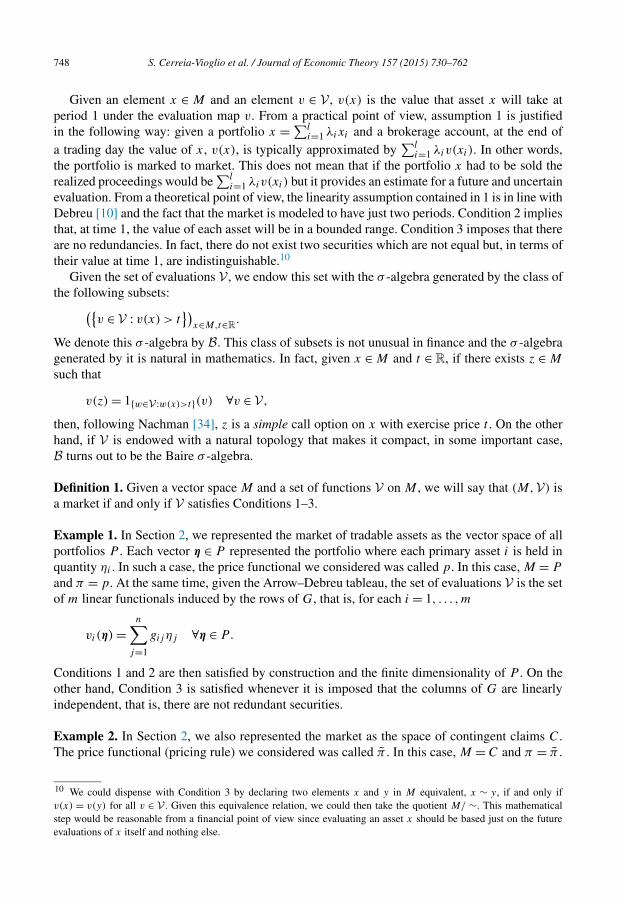
Given an element x ∈ M and an element v ∈ V , v(x) is the value that asset x will take at period 1 under the evaluation map v. From a practical point of view, assumption 1 is justified in the following way: given a portfolio x = ∑l
i=1 λixi and a brokerage account, at the end of a trading day the value of x, v(x), is typically approximated by
∑li=1 λiv(xi). In other words,
the portfolio is marked to market. This does not mean that if the portfolio x had to be sold the realized proceedings would be
∑li=1 λiv(xi) but it provides an estimate for a future and uncertain
evaluation. From a theoretical point of view, the linearity assumption contained in 1 is in line with Debreu [10] and the fact that the market is modeled to have just two periods. Condition 2 implies that, at time 1, the value of each asset will be in a bounded range. Condition 3 imposes that there are no redundancies. In fact, there do not exist two securities which are not equal but, in terms of their value at time 1, are indistinguishable.10
Given the set of evaluations V , we endow this set with the σ -algebra generated by the class of the following subsets:({
v ∈ V : v(x) > t})
x∈M,t∈R.
We denote this σ -algebra by B. This class of subsets is not unusual in finance and the σ -algebra generated by it is natural in mathematics. In fact, given x ∈ M and t ∈ R, if there exists z ∈ M
such that
v(z) = 1{w∈V :w(x)>t}(v) ∀v ∈ V,
then, following Nachman [34], z is a simple call option on x with exercise price t . On the other hand, if V is endowed with a natural topology that makes it compact, in some important case, B turns out to be the Baire σ -algebra.
Definition 1. Given a vector space M and a set of functions V on M , we will say that (M, V) is a market if and only if V satisfies Conditions 1–3.
Example 1. In Section 2, we represented the market of tradable assets as the vector space of all portfolios P . Each vector η ∈ P represented the portfolio where each primary asset i is held in quantity ηi . In such a case, the price functional we considered was called p. In this case, M = P
and π = p. At the same time, given the Arrow–Debreu tableau, the set of evaluations V is the set of m linear functionals induced by the rows of G, that is, for each i = 1, . . . , m
vi(η) =n∑
j=1
gij ηj ∀η ∈ P.
Conditions 1 and 2 are then satisfied by construction and the finite dimensionality of P . On the other hand, Condition 3 is satisfied whenever it is imposed that the columns of G are linearly independent, that is, there are not redundant securities.
Example 2. In Section 2, we also represented the market as the space of contingent claims C. The price functional (pricing rule) we considered was called π . In this case, M = C and π = π .
10 We could dispense with Condition 3 by declaring two elements x and y in M equivalent, x ∼ y, if and only if v(x) = v(y) for all v ∈ V . Given this equivalence relation, we could then take the quotient M/ ∼. This mathematical step would be reasonable from a financial point of view since evaluating an asset x should be based just on the future evaluations of x itself and nothing else.

S. Cerreia-Vioglio et al. / Journal of Economic Theory 157 (2015) 730–762 749
At the same time, given the state space Ω , the set of evaluations V is identified with the set of Dirac measures {δωi
}mi=1 and the linear functionals induced by each of these measures, that is, for each i = 1, . . . , m
vi(x) = xi ∀x ∈ C.
Conditions 1, 2, and 3 are then satisfied by construction.
B.2. Put–Call Parity and nonlinear pricing
Given a market (M, V) and an asset/portfolio x ∈ M , notice that x defines a function over V , that is,
v �→ v(x) v ∈ V .
One way in which the market could form a price for x, π(x), could be by discounting and averaging the possible evaluations of x at time 1 under a measure of likelihood ν : B → [0, 1]and a risk-free rate r ∈ (−1, ∞). This is what happens in a market with no frictions and no arbitrages. In such a case, ν is additive. This reasoning could be extended to the nonadditive case where the integrals are going to be defined using the concept of Choquet integration. In particular, we could have that
π(x) = 1
1 + r
∫V
v(x)dν(v) ∀x ∈ M. (21)
Our purpose is to characterize a price functional π : M → R like the one in (21) when minimal assumptions of no arbitrage are made and market frictions are also taken into account.
When modeling a market, the existence of a risk-free asset is often assumed. Such an asset has the fundamental feature of having a constant value at time 1. In particular, this value is independent of what might happen between time 0 and time 1. Therefore, in our context, we will define the risk-free asset in the following way:
Definition 2. An asset xrf in M is risk free if and only if
v(xrf ) = 1 ∀v ∈ V .
Another important type of financial assets are options: call and put. Those are derivative con-tracts since their value at time 1 is strictly related to the value of the underlying asset x. Those are securities that give the right to trade an asset x at time 1 at a fixed strike price k. The call option gives the right to buy while the put option the right to sell. The value at time 1 of a call option cx,k on x with strike price k depends on the value of x at time 1. For each valuation v ∈ V , it is v(x) − k if v(x) ≥ k and 0 otherwise. The value at time 1 of a put option px,k on x with strike price k depends on the value of x at time 1. For each valuation v ∈ V , it is k − v(x) if v(x) ≤ k
and 0 otherwise. Formally, we have that:
Definition 3. Let x be an asset in M . Then,
(i) cx,k is a call option on x with strike price k if and only if
v(cx,k) = (v(x) − k
)+ ∀v ∈ V .
750 S. Cerreia-Vioglio et al. / Journal of Economic Theory 157 (2015) 730–762
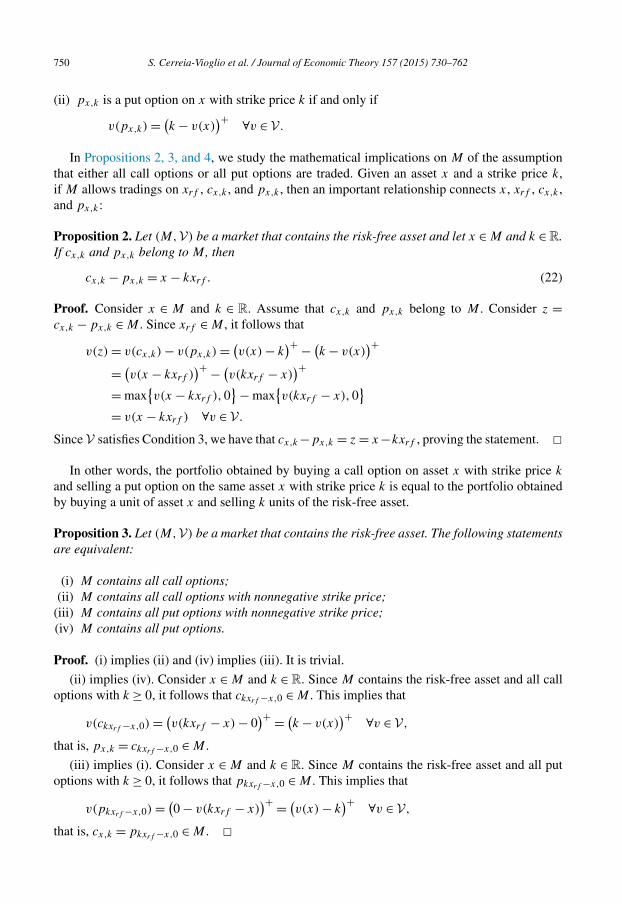
(ii) px,k is a put option on x with strike price k if and only if
v(px,k) = (k − v(x)
)+ ∀v ∈ V .
In Propositions 2, 3, and 4, we study the mathematical implications on M of the assumption that either all call options or all put options are traded. Given an asset x and a strike price k, if M allows tradings on xrf , cx,k , and px,k , then an important relationship connects x, xrf , cx,k , and px,k :
Proposition 2. Let (M, V) be a market that contains the risk-free asset and let x ∈ M and k ∈R. If cx,k and px,k belong to M , then
cx,k − px,k = x − kxrf . (22)
Proof. Consider x ∈ M and k ∈ R. Assume that cx,k and px,k belong to M . Consider z =cx,k − px,k ∈ M . Since xrf ∈ M , it follows that
v(z) = v(cx,k) − v(px,k) = (v(x) − k
)+ − (k − v(x)
)+
= (v(x − kxrf )
)+ − (v(kxrf − x)
)+
= max{v(x − kxrf ),0
} − max{v(kxrf − x),0
}= v(x − kxrf ) ∀v ∈ V .
Since V satisfies Condition 3, we have that cx,k −px,k = z = x−kxrf , proving the statement. �In other words, the portfolio obtained by buying a call option on asset x with strike price k
and selling a put option on the same asset x with strike price k is equal to the portfolio obtained by buying a unit of asset x and selling k units of the risk-free asset.
Proposition 3. Let (M, V) be a market that contains the risk-free asset. The following statements are equivalent:
(i) M contains all call options;(ii) M contains all call options with nonnegative strike price;
(iii) M contains all put options with nonnegative strike price;(iv) M contains all put options.
Proof. (i) implies (ii) and (iv) implies (iii). It is trivial.
(ii) implies (iv). Consider x ∈ M and k ∈ R. Since M contains the risk-free asset and all call options with k ≥ 0, it follows that ckxrf −x,0 ∈ M . This implies that
v(ckxrf −x,0) = (v(kxrf − x) − 0
)+ = (k − v(x)
)+ ∀v ∈ V,
that is, px,k = ckxrf −x,0 ∈ M .
(iii) implies (i). Consider x ∈ M and k ∈ R. Since M contains the risk-free asset and all put options with k ≥ 0, it follows that pkxrf −x,0 ∈ M . This implies that
v(pkxrf −x,0) = (0 − v(kxrf − x)
)+ = (v(x) − k
)+ ∀v ∈ V,
that is, cx,k = pkx −x,0 ∈ M . �
rf
S. Cerreia-Vioglio et al. / Journal of Economic Theory 157 (2015) 730–762 751
It is immediate to see that the set of evaluations V induces a partial order on M . In fact, it is reasonable to declare x at least as good as y if and only if the value of x at time 1 is greater than the value of y at time 1, irrespective of the evaluation function v chosen in V .
Definition 4. Let (M, V) be a market. We say that x is at least as good as y if and only if
v(x) ≥ v(y) ∀v ∈ V .
In this case, we write x ≥V y.
Given a market (M, V), differently from Brown and Ross [6], we do not assume that M is a vector lattice. On the contrary, by defining the primitive notions of call and put options, in the following proposition, we prove that a market (M, V), which contains the risk-free asset and all call options with nonnegative strike price, is a vector lattice with respect to ≥V . Given x ∈ M , we define x : V → R as x(v) = v(x) for all v ∈ V .
Proposition 4. Let (M, V) be a market. The following statements are true:
1. If M contains the risk-free asset xrf , then xrf is an order unit for (M, ≥V).2. If M contains the risk-free asset xrf and all call options with k ≥ 0, then (M, ≥V ) is a Riesz
space with unit. In particular, this implies that
cx,k + kxrf = x ∨ kxrf and cx,k = (x − kxrf ) ∨ 0 ∀x ∈ M, ∀k ∈ R
and
kxrf − px,k = x ∧ kxrf and px,k = (kxrf − x) ∨ 0 ∀x ∈ M, ∀k ∈R.
3. If M contains the risk-free asset xrf and all put options with k ≥ 0, then (M, ≥V ) is a Riesz space with unit.
4. If M contains the risk-free asset xrf and all call (resp., put) options with k ≥ 0, then
L = {f ∈RV : f = x for some x ∈ M
}is a Stone vector lattice.
5. If M contains the risk-free asset xrf and all call (resp., put) options with k ≥ 0, then the map T : M → L, defined by
x �→ x,
is a lattice isomorphism.
Proof. We define 〈·, ·〉 : V × M → R by 〈v, x〉 = v(x) for all v ∈ V and for all x ∈ M . Given an element x ∈ M , observe that x(v) = 〈v, x〉 for all v ∈ V . Since V satisfies Condition 2, we have that L ⊆ B(V). Given a market (M, V), we study the ordered space (M, ≥V). In such a context, given two elements x and y in M , we define, if they exist, the elements
x ∧ y = inf{x, y} and x ∨ y = sup{x, y}.
Step 1. ≥V is a partial order relation.
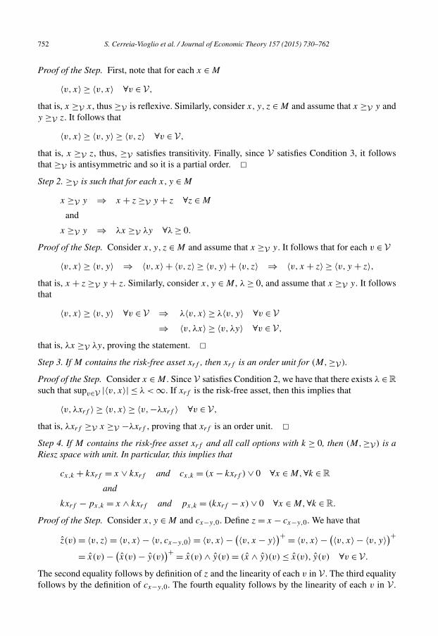
752 S. Cerreia-Vioglio et al. / Journal of Economic Theory 157 (2015) 730–762
Proof of the Step. First, note that for each x ∈ M
〈v, x〉 ≥ 〈v, x〉 ∀v ∈ V,
that is, x ≥V x, thus ≥V is reflexive. Similarly, consider x, y, z ∈ M and assume that x ≥V y and y ≥V z. It follows that
〈v, x〉 ≥ 〈v, y〉 ≥ 〈v, z〉 ∀v ∈ V,
that is, x ≥V z, thus, ≥V satisfies transitivity. Finally, since V satisfies Condition 3, it follows that ≥V is antisymmetric and so it is a partial order. �Step 2. ≥V is such that for each x, y ∈ M
x ≥V y ⇒ x + z ≥V y + z ∀z ∈ M
and
x ≥V y ⇒ λx ≥V λy ∀λ ≥ 0.
Proof of the Step. Consider x, y, z ∈ M and assume that x ≥V y. It follows that for each v ∈ V
〈v, x〉 ≥ 〈v, y〉 ⇒ 〈v, x〉 + 〈v, z〉 ≥ 〈v, y〉 + 〈v, z〉 ⇒ 〈v, x + z〉 ≥ 〈v, y + z〉,that is, x + z ≥V y + z. Similarly, consider x, y ∈ M , λ ≥ 0, and assume that x ≥V y. It follows that
〈v, x〉 ≥ 〈v, y〉 ∀v ∈ V ⇒ λ〈v, x〉 ≥ λ〈v, y〉 ∀v ∈ V⇒ 〈v,λx〉 ≥ 〈v,λy〉 ∀v ∈ V,
that is, λx ≥V λy, proving the statement. �Step 3. If M contains the risk-free asset xrf , then xrf is an order unit for (M, ≥V).
Proof of the Step. Consider x ∈ M . Since V satisfies Condition 2, we have that there exists λ ∈Rsuch that supv∈V |〈v, x〉| ≤ λ < ∞. If xrf is the risk-free asset, then this implies that
〈v,λxrf 〉 ≥ 〈v, x〉 ≥ 〈v,−λxrf 〉 ∀v ∈ V,
that is, λxrf ≥V x ≥V −λxrf , proving that xrf is an order unit. �Step 4. If M contains the risk-free asset xrf and all call options with k ≥ 0, then (M, ≥V ) is a Riesz space with unit. In particular, this implies that
cx,k + kxrf = x ∨ kxrf and cx,k = (x − kxrf ) ∨ 0 ∀x ∈ M,∀k ∈ R
and
kxrf − px,k = x ∧ kxrf and px,k = (kxrf − x) ∨ 0 ∀x ∈ M,∀k ∈ R.
Proof of the Step. Consider x, y ∈ M and cx−y,0. Define z = x − cx−y,0. We have that
z(v) = 〈v, z〉 = 〈v, x〉 − 〈v, cx−y,0〉 = 〈v, x〉 − (〈v, x − y〉)+ = 〈v, x〉 − (〈v, x〉 − 〈v, y〉)+
= x(v) − (x(v) − y(v)
)+ = x(v) ∧ y(v) = (x ∧ y)(v) ≤ x(v), y(v) ∀v ∈ V .
The second equality follows by definition of z and the linearity of each v in V . The third equality follows by the definition of cx−y,0. The fourth equality follows by the linearity of each v in V .

S. Cerreia-Vioglio et al. / Journal of Economic Theory 157 (2015) 730–762 753
The fifth equality follows by definition of x and y. The sixth equality follows from a well known lattice equality (see [2, Theorem 1.7]).
We can conclude that x, y ≥V z. Next, assume that w ∈ M is such that x, y ≥V w. By defini-tion of ≥V and the previous part, it follows that
x(v), y(v) ≥ w(v) ∀v ∈ V ⇒ 〈v, z〉 = (x ∧ y)(v) ≥ w(v) = 〈v,w〉 ∀v ∈ V .
This implies that z ≥V w, that is, z is the greatest lower bound for x and y and z = x ∧ y. By Steps 1, 2, and 3, (M, ≥V ) is an ordered vector space with unit. This fact matched with the previous one implies that (M, ≥V) is a Riesz space with unit. Next, consider x ∈ M and k ∈ R. It is immediate to check that cx,k = cx−kxrf ,0. It follows that
cx,k + kxrf = cx−kxrf ,0 + kxrf = (x − x ∧ kxrf ) + kxrf
= x + kxrf − x ∧ kxrf = x ∨ kxrf ,
where the first equality is trivial, the second one follows from the previous part of the proof, that is, cx−y,0 = x − x ∧ y, the third follows from a simple rearrangement, and the fourth one is a well known lattice equality (see [1, Theorem 8.6]). On the other hand, from above we have that cx,k = x ∨ kxrf − kxrf = (x − kxrf ) ∨ 0. A similar argument delivers the equalities
kxrf − px,k = x ∧ kxrf and px,k = (kxrf − x) ∨ 0 ∀x ∈ M, ∀k ∈R. �Step 5. If M contains the risk-free asset xrf and all put options with k ≥ 0, then (M, ≥V ) is a Riesz space with unit.
Proof of the Step. By Proposition 3, M contains all call options with k ≥ 0. By Step 4, the statement follows. �Step 6. The map T : M → L, defined by
x �→ x,
is a bijective linear operator. In particular, L is a vector space and if M contains the risk-free asset xrf , then L contains the constant functions.
Proof of the Step. By construction, the map T is surjective. On the other hand, if we have that T (x1) = T (x2), then it follows that
〈v, x1〉 = x1(v) = x2(v) = 〈v, x2〉 ∀v ∈ V . (23)
Since V satisfies Condition 3, (23) implies that x1 = x2, proving that T is injective. Next, given x, y ∈ M and λ, μ ∈R, we have that
T (λx + μy)(v) = 〈v,λx + μy〉 = λ〈v, x〉 + μ〈v, y〉 = λT (x)(v) + μT (y)(v) ∀v ∈ V,
that is, T (λx + μy) = λT (x) + μT (y), proving that T is linear. Since M is a vector space and T is linear and bijective, L is a vector space. At the same time, if xrf is the risk-free asset and xrf ∈ M , then 1V = T (xrf ) ∈ L. Since L is a vector space, it follows that L contains all constant functions. �Step 7. If M contains the risk-free asset xrf and all call (resp., put) options with k ≥ 0, then L is a Stone vector lattice.
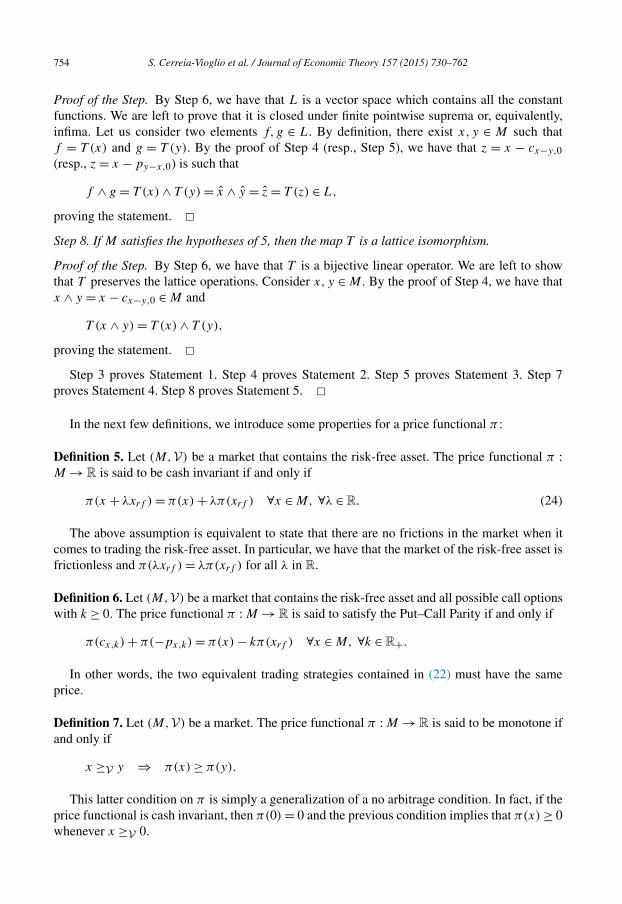
754 S. Cerreia-Vioglio et al. / Journal of Economic Theory 157 (2015) 730–762
Proof of the Step. By Step 6, we have that L is a vector space which contains all the constant functions. We are left to prove that it is closed under finite pointwise suprema or, equivalently, infima. Let us consider two elements f, g ∈ L. By definition, there exist x, y ∈ M such that f = T (x) and g = T (y). By the proof of Step 4 (resp., Step 5), we have that z = x − cx−y,0(resp., z = x − py−x,0) is such that
f ∧ g = T (x) ∧ T (y) = x ∧ y = z = T (z) ∈ L,
proving the statement. �Step 8. If M satisfies the hypotheses of 5, then the map T is a lattice isomorphism.
Proof of the Step. By Step 6, we have that T is a bijective linear operator. We are left to show that T preserves the lattice operations. Consider x, y ∈ M . By the proof of Step 4, we have that x ∧ y = x − cx−y,0 ∈ M and
T (x ∧ y) = T (x) ∧ T (y),
proving the statement. �Step 3 proves Statement 1. Step 4 proves Statement 2. Step 5 proves Statement 3. Step 7
proves Statement 4. Step 8 proves Statement 5. �In the next few definitions, we introduce some properties for a price functional π :
Definition 5. Let (M, V) be a market that contains the risk-free asset. The price functional π :M →R is said to be cash invariant if and only if
π(x + λxrf ) = π(x) + λπ(xrf ) ∀x ∈ M, ∀λ ∈ R. (24)
The above assumption is equivalent to state that there are no frictions in the market when it comes to trading the risk-free asset. In particular, we have that the market of the risk-free asset is frictionless and π(λxrf ) = λπ(xrf ) for all λ in R.
Definition 6. Let (M, V) be a market that contains the risk-free asset and all possible call options with k ≥ 0. The price functional π : M → R is said to satisfy the Put–Call Parity if and only if
π(cx,k) + π(−px,k) = π(x) − kπ(xrf ) ∀x ∈ M, ∀k ∈ R+.
In other words, the two equivalent trading strategies contained in (22) must have the same price.
Definition 7. Let (M, V) be a market. The price functional π : M → R is said to be monotone if and only if
x ≥V y ⇒ π(x) ≥ π(y).
This latter condition on π is simply a generalization of a no arbitrage condition. In fact, if the price functional is cash invariant, then π(0) = 0 and the previous condition implies that π(x) ≥ 0whenever x ≥V 0.

S. Cerreia-Vioglio et al. / Journal of Economic Theory 157 (2015) 730–762 755
Example 3. In Section 2, we represented the market of tradable assets as the vector space of all portfolios P and also as the vector space of all tradable contingent claims C. In the first case, Example 1, we have that V is the set of linear evaluations induced by the rows of the Arrow–Debreu tableau G. It follows that a portfolio ηrf corresponds to the risk-free asset if and only if Gηrf is the constant vector with each component equal to 1. Similarly, given a portfolio η, a call (resp., a put) option on η with strike price k is the portfolio cη,k (resp., pη,k) such that
Gcη,k = (Gη − kGηrf )+ = max{Gη − kGηrf ,0}(resp., Gpη,k = (kGηrf − Gη)+ = max{kGηrf − Gη,0}).
Finally, a discount certificate on a portfolio η with cap k ≥ 0 is the portfolio dη,k such that
Gdη,k = min{Gη, kGηrf }.Moreover, we have that ≥V is equal to ≥G. Along the same lines, we have that cη,k (resp., pη,k) is the positive part, with respect to ≥G, of the vector η − kηrf (resp., kηrf − η). On the other hand, dη,k is the minimum, with respect to ≥G, between η and kηrf . The price functional psatisfies PCP if and only if
p(cη,k) + p(−pη,k) = p(η) − kp(ηrf ) ∀η ∈ P, ∀k ≥ 0. (25)
Similarly, p is cash invariant if and only if
p(η + kηrf ) = p(η) + kp(ηrf ) ∀η ∈ P, ∀k ∈ R. (26)
Finally, p satisfies DCP if and only if
p(cη,k) + p(dη,k) = p(η) ∀η ∈ P, ∀k ≥ 0. (27)
In the second case, Example 2, we have that V is the set of linear functionals induced by the Dirac measures on Ω . In this case, we have that a contingent claim xrf corresponds to the risk-free asset if and only if it is the constant vector with each component equal to 1. Similarly, given a contingent claim x, a call (resp., a put) on x with strike price k is the portfolio cx,k (resp., px,k) such that
cx,k = (x − kxrf )+(resp., px,k = (kxrf − x)+
).
Moreover, we have that ≥V coincides with the usual pointwise order.
Proposition 5. Let (M, V) be a market that contains the risk-free asset and all call options with k ≥ 0 and let π : M → R be a cash invariant price functional. The following conditions are equivalent:
(i) π(cx,k) + π(−px,k) = π(x) − kπ(xrf ) for all x ∈ M and all k ∈ R+;(ii) π(x ∨ kxrf ) + π(x ∧ kxrf ) = π(x) + kπ(xrf ) for all x ∈ M and all k ∈ R+;
(iii) π(x ∨ kxrf ) + π(x ∧ kxrf ) = π(x) + kπ(xrf ) for all x ∈ M and all k ∈ R.
Proof. (i) implies (iii). Consider x ∈ M and k ∈ R. By Proposition 4 point 2, we have that
cx,k + kxrf = x ∨ kxrf and kxrf − px,k = x ∧ kxrf .
Since π is cash invariant, cx,k = cx−kxrf ,0, and px,k = px−kxrf ,0, we have the following chain of implications

756 S. Cerreia-Vioglio et al. / Journal of Economic Theory 157 (2015) 730–762
π(cx−kxrf ,0) + π(−px−kxrf ,0) = π(x − kxrf )
�⇒π(cx,k) + π(−px,k) = π(x) − kπ(xrf )
�⇒π(cx,k) + kπ(xrf ) + π(−px,k) + kπ(xrf ) = π(x) + kπ(xrf )
�⇒π(cx,k + kxrf ) + π(kxrf − px,k) = π(x) + kπ(xrf )
�⇒π(x ∨ kxrf ) + π(x ∧ kxrf ) = π(x) + kπ(xrf ),
proving the statement.
(iii) implies (ii). It is trivial.
(ii) implies (i). Consider x ∈ M and k ∈ R+. By Proposition 4 point 2, M is a Riesz space with unit. This implies that
x ∨ kxrf − kxrf = (x − kxrf ) ∨ 0 = cx,k and
x ∧ kxrf − kxrf = (x − kxrf ) ∧ 0 = −px,k.
Since π is cash invariant, we have the following chain of implications
π(x ∨ kxrf ) + π(x ∧ kxrf ) = π(x) + kπ(xrf )
�⇒π(x ∨ kxrf ) − kπ(xrf ) + π(x ∧ kxrf ) − kπ(xrf ) = π(x) − kπ(xrf )
�⇒π(x ∨ kxrf − kxrf ) + π(x ∧ kxrf − kxrf ) = π(x) − kπ(xrf )
�⇒π(cx,k) + π(−px,k) = π(x) − kπ(xrf ),
proving the statement. �Before stating the main result, we need to introduce two new objects: ν�, ν� : B → [0, 1],
defined by
ν�(A) = sup{π(x) : x ≤V 1A}π(xrf )
and ν�(A) = inf{π(x) : x ≥V 1A}π(xrf )
,
where π(xrf ) is assumed to be different from zero.
Theorem 3. Let (M, V) be a market that contains the risk-free asset and all call options with k ≥ 0 and let π : M →R be a nonzero price functional. The following statements are equivalent:
(i) π is monotone, cash invariant, and satisfies the Put–Call Parity;

S. Cerreia-Vioglio et al. / Journal of Economic Theory 157 (2015) 730–762 757
(ii) there exist a nonadditive probability ν : B → [0, 1] and a risk-free rate r > −1 such that
π(x) = 1
1 + r
∫V
v(x)dν(v) ∀x ∈ M. (28)
Moreover,
1. r is unique.2. Each nonadditive probability ν : B → [0, 1] that satisfies ν� ≤ ν ≤ ν� represents π as in (28).3. If B(V, B) = {x : x ∈ M}, then ν is unique.4. If ν is balanced, then π(x) ≥ −π(−x) for all x ∈ M , that is, there are positive bid–ask
spreads.
Proof. Before starting, observe that σ(L) = B.(i) implies (ii). Define I : L → R by I = π ◦ T −1. Since T is a lattice isomorphism such that
T (xrf ) = 1V and π = 0, it follows that I is well defined, monotone, translation invariant, and such that I = 0. Since π satisfies the Put–Call Parity and by Proposition 5, we have that
π(x ∧ kxrf ) + π(x ∨ kxrf ) = π(x) + kπ(xrf ) ∀x ∈ M, ∀k ∈R. (29)
Since T is a lattice isomorphism and T (xrf ) = 1V , this implies that I is constant modular. By Theorem 2 and since L is a Stone vector lattice, we have that there exist δ > 0 and a nonad-ditive probability ν : B → [0, 1] such that
I (f ) = δ
∫V
f (v)dν(v) ∀f ∈ L.
Define r = 1/δ − 1 > −1. Since π = I ◦ T , we have that
π(x) = I(T (x)
) = 1
1 + r
∫V
〈v, x〉dν(v) = 1
1 + r
∫V
v(x)dν(v) ∀x ∈ M,
proving the statement.
(ii) implies (i). Consider r > −1 and a nonadditive probability ν : B → [0, 1] such that
π(x) = 1
1 + r
∫V
v(x)dν(v) ∀x ∈ M.
Define I : L →R by
I (f ) = δ
∫V
f (v)dν(v) ∀f ∈ L (30)
where δ = 1/(1 + r). By Theorem 2, we have that I is monotone, translation invariant, and constant modular. It is immediate to see that π = I ◦ T . Since T is a lattice isomorphism and T (xrf ) = 1V , it follows that π is monotone, cash invariant, and it satisfies (29). By Proposition 5, it follows that π also satisfies the Put–Call Parity.

758 S. Cerreia-Vioglio et al. / Journal of Economic Theory 157 (2015) 730–762
1. Consider r1, r2 > −1 and ν1, ν2 : B → [0, 1] such that
π(x) = 1
1 + ri
∫V
v(x)dνi(v) ∀x ∈ M, ∀ i ∈ {1,2}.
It follows that 11+r1
= π(xrf ) = 11+r2
, proving that r1 = r2 and so the statement.
2. Consider a nonadditive probability ν : B → [0, 1] such that ν� ≤ ν ≤ ν�. Define I = π ◦ T −1. It follows that ν� = ν∗ and ν� = ν∗. This implies that ν∗ ≤ ν ≤ ν∗. By Theorem 2, we have that I (f ) = I (1V )
∫V f dν for all f ∈ L. Since π = I ◦ T , the statement follows.
3. Assume that B(V, B) = {x : x ∈ M}. It follows that for each A ∈ B there exists xA ∈ M
such that v(x) = 1A(v) for all v ∈ V . Consider (r1, ν1) and (r2, ν2) representing π as in (28). By point 1, we have that r1 = r2 and
1
1 + r1ν1(A) = π(xA) = 1
1 + r2ν2(A) ∀A ∈ B.
This implies that ν1 = ν2, proving the statement.
4. Consider (r, ν) representing π as in (28). Define ν : B → [0, 1] by
ν(A) = ν(V) − ν(Ac
) ∀A ∈ B.
Assume that ν is balanced. It follows that there exists μ ∈ �(V) such that μ(A) ≤ ν(A) for all A ∈ B. This implies that ν(A) ≤ μ(A) for all A ∈ B. By [33, Proposition 4.12], if we define I as in (30), then
−I (−f ) = 1
1 + r
∫V
f (v)dν(v) ∀f ∈ L.
By the definition of Choquet integral and since ν ≤ μ ≤ ν, it follows that −I (−f ) ≤1
1+r
∫V f (v)dμ(v) ≤ I (f ) for all f ∈ L. Since π = I ◦ T and T is linear, we have that
−π(−x) = −I(−T (x)
) ≤ I(T (x)
) = π(x) ∀x ∈ M,
proving the statement. �When (M, V) is as in Example 2, Theorem 3 naturally yields the equivalence of points (i) and
(iii) in Theorem 1. On the other hand, when (M, V) is as in Example 1, Theorem 3 yields the generalization of the Fundamental Theorem of Finance once it is applied to the price functional p and three facts are noticed:
(a) p has a representation as in (28) where V is the set of rows of the Arrow–Debreu tableau G;(b) thus, p satisfies monotonicity, translation invariance, and constant modularity with respect
to ≥G;(c) by monotonicity with respect to ≥G, the Law of One Price holds. Since T , defined as in
Section 2, is a lattice isomorphism, it follows that πp = p ◦ T −1. It also follows that πp
satisfies monotonicity, translation invariance, and constant modularity with respect to the usual order ≥.

S. Cerreia-Vioglio et al. / Journal of Economic Theory 157 (2015) 730–762 759
B.3. The subadditive case
One way in which the literature introduced transaction costs in pricing has been by considering subadditive price functionals and pricing rules (see Jouini and Kallal [26] and Luttmer [32]).
Definition 8. Let (M, V) be a market. The price functional π : M → R is said to be subadditive if and only if
π(x + y) ≤ π(x) + π(y) ∀x, y ∈ M.
If π is cash invariant, this assumption is particularly important since it implies the existence of positive bid–ask spreads. In fact, we have that π(x) + π(−x) ≥ π(0) = 0 for all x ∈ M . In this context, the assumptions of cash invariance and monotonicity, contained in Definition 5 and Definition 7, can be weakened to be the following notion of linearity and positivity:
Definition 9. Let (M, V) be a market. The price functional π : M → R is said to be normalized if and only if
π(kxrf ) = kπ(xrf ) ∀k ∈ R.
Definition 10. Let (M, V) be a market. The price functional π : M → R is said to be negative if and only if
0 ≥V x ⇒ 0 ≥ π(x).
Corollary 2. Let (M, V) be a market that contains the risk-free asset and all call options with k ≥ 0 and let π : M → R be a nonzero price functional. The following statements are equivalent:
(i) π is negative, normalized, subadditive, and satisfies the Put–Call Parity;(ii) π is monotone, cash invariant, subadditive, and satisfies the Put–Call Parity;
(iii) there exist a concave nonadditive probability ν : B → [0, 1] and a risk-free rate r > −1such that
π(x) = 1
1 + r
∫V
v(x)dν(v) ∀x ∈ M.
Moreover, r is unique and ν can be chosen to be ν�.
Proof. (i) implies (ii). We only need to show that π is monotone and cash invariant. If x, y ∈ M
are such that y ≥V x, then 0 ≥V x − y. Since π is subadditive and negative, it follows that
π(x) = π(y + (x − y)
) ≤ π(y) + π(x − y) ≤ π(y),
proving that π is monotone. Similarly, since π is subadditive and normalized, we have that
π(x + kxrf ) ≤ π(x) + π(kxrf ) = π(x) + kπ(xrf ) ∀x ∈ M, ∀k ∈ R. (31)
By (31), we also have that
π(x) = π((x + kxrf ) − kxrf
) ≤ π(x + kxrf ) − kπ(xrf ) ∀x ∈ M, ∀k ∈ R. (32)
The inequalities in (31) and (32) imply that π is cash invariant.

760 S. Cerreia-Vioglio et al. / Journal of Economic Theory 157 (2015) 730–762
(ii) implies (iii). Define I : L → R by I = π ◦ T −1. By the same argument contained in the proof of Theorem 3, we have that I is well defined, monotone, translation invariant, constant modular, and such that I = 0. Since π is subadditive and T is a lattice isomorphism, we have that I is also subadditive. By Theorem 2 and since L is a Stone vector lattice, we have that there exists δ > 0 such that
I (f ) = δ
∫V
f (v)dν∗(v) ∀f ∈ L.
By Theorem 2 and since I is subadditive, we have that ν∗ = ν� is concave. Define r = 1/δ − 1. Since π = I ◦ T , we have that
π(x) = 1
1 + r
∫V
〈v, x〉dν∗(v) = 1
1 + r
∫V
v(x)dν�(v) ∀x ∈ M,
proving the statement.
(iii) implies (i). Consider r > −1 and a concave nonadditive probability ν : B → [0, 1] such that
π(x) = 1
1 + r
∫V
v(x)dν(v) ∀x ∈ M.
Define I : L → R as in (30) where δ = 1/(1 + r). By Theorem 2, we have that I is monotone, translation invariant, and constant modular. Since ν is concave and by [33, Theorem 4.6], I is also subadditive. It is immediate to see that π = I ◦ T . Since T is a lattice isomorphism and T (xrf ) = 1V , it follows that π is monotone, cash invariant, subadditive, and it satisfies (29). By Proposition 5, it follows that π also satisfies the Put–Call Parity. Since π(0) = 0 and π is monotone, it follows that π is negative. Since π is cash invariant, it follows that π is normalized.
Uniqueness of r > −1 follows from Theorem 3 and the fact that ν can be chosen to be ν�
follows from the previous part of the proof. �Our last result allows us to discuss uniqueness of the nonadditive probability ν also when the
market does not span the entire space of all contingent claims, that is, {x : x ∈ M} = B(V, B). In order to do so, we need to introduce a notion of continuity for the price functional π .11
Definition 11. Let (M, V) be a market. The price functional π : M → R is said to be continuous if and only if for each sequence {xn}n∈N ⊆ M we have that
limn
v(xn) = 0 ∀v ∈ V ⇒ limn
π(xn) = 0,
provided there exists l ∈ R such that |v(xn)| ≤ l for all v ∈ V and for all n ∈N.
Corollary 3. Let (M, V) be a market that contains the risk-free asset and all call options with k ≥ 0 and let π : M →R be a nonzero price functional. The following statements are equivalent:
(i) π is negative, normalized, subadditive, continuous, and satisfies the Put–Call Parity;
11 In reading Definition 11, notice that continuity is required with respect to the bounded weak convergence induced by V .

S. Cerreia-Vioglio et al. / Journal of Economic Theory 157 (2015) 730–762 761
(ii) there exist a continuous and concave nonadditive probability ν : B → [0, 1] and a risk-free rate r > −1 such that
π(x) = 1
1 + r
∫V
v(x)dν(v) ∀x ∈ M.
Moreover, r and ν are unique.
Proof. Before starting the proof, we introduce a third point:(iii) π is monotone, cash invariant, subadditive, continuous, and satisfies the Put–Call Parity.
(i) implies (iii). The statement follows by the same arguments used in the proof of Corollary 2.
(iii) implies (ii). Define I : L → R by I = π ◦ T −1. By the same argument contained in the proof of Corollary 2, we have that I is well defined, monotone, translation invariant, constant modular, subadditive, and such that I = 0. Since π is continuous and T is a lattice isomorphism, we have that I is also pointwise continuous at 0. By Theorem 2 and since L is a Stone vector lattice, we have that there exist a continuous and concave nonadditive probability ν : B → [0, 1]and δ > 0 such that
I (f ) = δ
∫V
f (v)dν(v) ∀f ∈ L.
Define r = 1/δ − 1. Since π = I ◦ T , we have that
π(x) = 1
1 + r
∫V
〈v, x〉dν(v) = 1
1 + r
∫V
v(x)dν(v) ∀x ∈ M,
proving the statement.
(ii) implies (i). Consider r > −1 and a continuous and concave nonadditive probability ν :B → [0, 1] such that
π(x) = 1
1 + r
∫V
v(x)dν(v) ∀x ∈ M.
Define I : L →R as in (30) where δ = 1/(1 + r). By Theorem 2 and [33, Theorem 4.6], we have that I is monotone, translation invariant, constant modular, subadditive, and pointwise continu-ous at 0. It is immediate to see that π = I ◦T . Since T is a lattice isomorphism and T (xrf ) = 1V , it follows that π is monotone, cash invariant, subadditive, continuous, and it satisfies (29). By Proposition 5, it follows that π also satisfies the PCP. Since π(0) = 0 and π is monotone, it fol-lows that π is negative. Since π is cash invariant, it follows that π is normalized.
Uniqueness of r > −1 and ν follows from Theorem 2. �References
[1] C.D. Aliprantis, K.C. Border, Infinite Dimensional Analysis, 3rd ed., Springer Verlag, Berlin, 2006.[2] C.D. Aliprantis, O. Burkinshaw, Positive Operators, 2nd ed., Springer, Dordrecht, 2006.[3] Y. Amihud, H. Mendelson, Asset pricing and the bid–ask spread, J. Finan. Econ. 17 (1986) 223–249.[4] Y. Amihud, H. Mendelson, Liquidity, maturity, and the yields on U.S. Treasury securities, J. Finance 56 (1991)
1411–1425.

762 S. Cerreia-Vioglio et al. / Journal of Economic Theory 157 (2015) 730–762
[5] F.J. Anscombe, R.J. Aumann, A definition of subjective probability, Ann. Math. Stat. 34 (1963) 199–205.[6] D.J. Brown, S.A. Ross, Spanning, valuation and options, Econ. Theory 1 (1991) 3–12.[7] S. Cerreia-Vioglio, F. Maccheroni, M. Marinacci, L. Montrucchio, Signed integral representations of comonotonic
additive functionals, J. Math. Anal. Appl. 385 (2012) 895–912.[8] A. Chateauneuf, R. Kast, A. Lapied, Choquet pricing for financial markets with frictions, Math. Finance 6 (1996)
323–330.[9] J.C. Cox, S.A. Ross, A survey of some new results in financial option pricing theory, J. Finance 31 (1976) 383–402.
[10] G. Debreu, Valuation equilibrium and Pareto optimum, Proc. Natl. Acad. Sci. 40 (1954) 588–592.[11] F. Delbaen, W. Schachermayer, A general version of the fundamental theorem of asset pricing, Math. Ann. 300
(1994) 463–520.[12] F. Delbaen, W. Schachermayer, The Mathematics of Arbitrage, Springer, Berlin, 2006.[13] D. Denneberg, Non-Additive Measure and Integral, Kluwer, Dordrecht, 1994.[14] P.H. Dybvig, S.A. Ross, Arbitrage, in: New Palgrave: A Dictionary of Economics, MacMillan, London, 1987.[15] D. Ellsberg, Risk, ambiguity, and the savage axioms, Quart. J. Econ. 75 (1961) 643–669.[16] H. Follmer, A. Schied, Stochastic Finance: An Introduction in Discrete Time, 2nd ed., De Gruyter, Berlin, 2004.[17] M.B. Garman, J.A. Ohlson, Valuation of risky assets in arbitrage-free economies with transaction costs, J. Finan.
Econ. 9 (1981) 271–280.[18] I. Gilboa, Expected utility with purely subjective non-additive probabilities, J. Math. Econ. 16 (1987) 65–88.[19] I. Gilboa, M. Marinacci, Ambiguity and the Bayesian paradigm, in: D. Acemoglu, M. Arellano, E. Dekel (Eds.),
Advances in Economics and Econometrics, vol. 1, Cambridge University Press, Cambridge, 2013, pp. 179–242.[20] J.P. Gould, D. Galai, Transactions costs and the relationship between put and call prices, J. Finan. Econ. 1 (1974)
105–129.[21] G.H. Greco, Sulla rappresentazione di funzionali mediante integrali, in: Rendiconti Seminario Matematico Univer-
sità di Padova, vol. 66, 1982, pp. 21–42.[22] R.C. Green, R.A. Jarrow, Spanning and completeness in markets with contingent claims, J. Econ. Theory 41 (1987)
202–210.[23] J.M. Harrison, D.M. Kreps, Martingales and arbitrage in multiperiod securities markets, J. Econ. Theory 20 (1979)
381–408.[24] J.M. Harrison, S.R. Pliska, Martingales and stochastic integrals in the theory of continuous trading, Stoch. Process.
Appl. 11 (1981) 215–260.[25] R.A. Jarrow, M. O’Hara, Primes and scores: an essay on market imperfection, J. Finance 44 (1989) 1263–1287.[26] E. Jouini, H. Kallal, Martingales and arbitrage in securities markets with transaction costs, J. Econ. Theory 66
(1995) 178–197.[27] Y. Kabanov, M. Safarian, Markets with Transaction Costs, Springer Verlag, Berlin, 2009.[28] A. Kamara, T.W. Miller, Daily and intradaily tests of European Put–Call Parity, J. Finan. Quant. Anal. 30 (1995)
519–539.[29] R.C. Klemkosky, B.G. Resnick, An ex ante analysis of Put–Call Parity, J. Finan. Econ. 8 (1980) 363–378.[30] R.J. Kruizenga, Put and call options: a theoretical and market analysis, PhD thesis, MIT, Cambridge, 1956.[31] S.F. LeRoy, J. Werner, Principles of Financial Economics, Cambridge University Press, Cambridge, 2001.[32] E.G.J. Luttmer, Asset pricing in economies with frictions, Econometrica 64 (1996) 363–378.[33] M. Marinacci, L. Montrucchio, Introduction to the mathematics of ambiguity, in: I. Gilboa (Ed.), Uncertainty in
Economic Theory, Routledge, New York, 2004.[34] D.C. Nachman, Spanning and completeness with options, Rev. Finan. Stud. 1 (1989) 311–328.[35] E.Z. Prisman, Valuation of risky assets in arbitrage free economies with frictions, J. Finance 56 (1986) 545–557.[36] S. Ross, Return, risk and arbitrage, Wharton discussion paper, Working paper number 17–73b, 1973.[37] S. Ross, Options and efficiency, Quart. J. Econ. 90 (1976) 75–89.[38] S. Ross, A simple approach to the valuation of risky streams, J. Bus. 51 (1978) 453–475.[39] S. Ross, Arbitrage and martingales with taxation, J. Polit. Econ. 95 (1987) 371–393.[40] S. Ross, Neoclassical Finance, Princeton University Press, Princeton, 2005.[41] L.J. Savage, The Foundations of Statistics, Wiley, New York, 1954.[42] D. Schmeidler, Integral representation without additivity, Proc. Amer. Math. Soc. 97 (1986) 255–261.[43] D. Schmeidler, Subjective probability and expected utility without additivity, Econometrica 57 (1989) 571–587.[44] H.R. Stoll, The relationship between put and call option prices, J. Finance 24 (1969) 801–824.[45] H.R. Stoll, The relationship between put and call option prices: reply, J. Finance 28 (1973) 185–187.