real-time model predictive control based on dual...

INTERNATIONAL JOURNAL OF ROBUST AND NONLINEAR CONTROLInt. J. Robust Nonlinear Control 2016; 26:3292–3310Published online 12 January 2016 in Wiley Online Library (wileyonlinelibrary.com). DOI: 10.1002/rnc.3507

Real-time model predictive control based on dual gradientprojection: Theory and fixed-point FPGA implementation

Matteo Rubagotti1,*,† , Panagiotis Patrinos2, Alberto Guiggiani3 and Alberto Bemporad3

1Department of Engineering, University of Leicester, University Rd, Leicester, UK2Department of Electrical Engineering (ESAT), STADIUS Center for Dynamical Systems, Signal Processing and Data

Analytics, Katholieke Universiteit Leuven, Leuven 3001, Belgium3IMT Institute for Advanced Studies, Lucca 55100, Italy

SUMMARY

This paper proposes a method to design robust model predictive control (MPC) laws for discrete-time linearsystems with hard mixed constraints on states and inputs, in case of only an inexact solution of the associ-ated quadratic program is available, because of real-time requirements. By using a recently proposed dualgradient-projection algorithm, it is proved that the discrepancy of the optimal control law as compared withthe obtained one is bounded even if the solver is implemented in fixed-point arithmetic. By defining an alter-native MPC problem with tightened constraints, a feasible solution is obtained for the original MPC problem,which guarantees recursive feasibility and asymptotic stability of the closed-loop system with respect to aset including the origin, also considering the presence of external disturbances. The proposed MPC law isimplemented on a field-programmable gate array in order to show the practical applicability of the method.Copyright © 2016 John Wiley & Sons, Ltd.

Received 12 June 2014; Revised 23 August 2015; Accepted 30 November 2015

KEY WORDS: model predictive control; uncertain systems; optimization methods

1. INTRODUCTION

Model predictive control (MPC) allows the design of optimal feedback control laws for dynamicalsystems that take into account constraints on inputs and states [1]. Thanks to the accomplish-ments of the last years in increasing both the computation capabilities of microcontrollers and theefficiency of fast algorithms for online optimization, the use of MPC is being extended from the tra-ditional process control applications to fields like automotive, aerospace, and mechatronics, whererelatively fast sampling times are required. In order to implement embedded MPC controllers forthis kind of systems, the worst-case execution time at each sampling time must be known, that is,real-time guarantees are needed. To this aim, real-time MPC laws have been recently proposed,studying optimization algorithms that generate an acceptable solution in an a priori bounded numberof iterations.

When a linear model of the system is employed, together with a quadratic cost function and linearconstraints, the optimization problem to be solved online can be formulated as a quadratic program(QP). In order to provide a solution of the QP in a prescribed time, two different strategies havebeen considered. The first consists of using the so-called explicit MPC approach introduced in [2],in which the optimal control law is explicitly obtained during the design phase as a piecewise affinefunction of the state vector by means of parametric optimization. For small-size problems, such

*Correspondence to: Matteo Rubagotti, Department of Engineering, University of Leicester, University Rd, LeicesterLE1 7RH, UK.

†E-mail: [email protected]

Copyright © 2016 John Wiley & Sons, Ltd.

REAL-TIME MPC BASED ON GPD: THEORY AND FIXED-POINT FPGA IMPLEMENTATION 3293

a function can be easily implemented in embedded control systems, giving a precise estimate ofthe worst-case execution time. Conversely, if the problem is of medium or large size, then onlineoptimization has to be employed. Using standard solvers, based on interior-point or active-set meth-ods, the estimate of the worst-case execution time is usually extremely loose (see, for instance, thediscussion in [3, Section IA]). For this reason, algorithms based on variants of the fast gradientmethods [4, 5] have been recently applied to MPC in [3, 6–8], providing tighter bounds. In [9], adual gradient-projection method based on [4] was proposed both in its basic (GPD) and accelerated(GPAD) forms (see also [10]). Despite introducing a dual method, [9] provides bounds on the maxi-mum number of iterations in order to achieve given levels of primal suboptimality and infeasibility.In [11], the use of GPD was analyzed for embedded MPC in hardware platforms with fixed-pointarithmetic.

In case a primal method is used, the obtained suboptimal solution does not violate the inequalityconstraints of the finite-horizon optimal control problem, and closed-loop stability can be provedusing, for instance, the method described in [12]. However, the use of primal methods is lim-ited to problems with simple input constraints, such as box constraints and no state constraints(e.g., [3]). Dual methods (e.g., [9, 13–16]) have been successfully applied to more general problemformulations (with polytopic mixed constraints on input and state variables), but they present thedrawback of providing inexact solutions for the associated primal problem because the inequalityconstraints can be violated. Possible solutions to this drawback were recently proposed in [17–19].The approaches of [14, 17] do not provide a priori bounds on the maximum number of iterationsvalid for the entire region of attraction, which are instead provided in [19]. In particular, in [19],starting from the MPC problem to be solved online, and given the maximum constraint violationand suboptimality of the solution provided by the solver (e.g., GPAD), an alternative problem isformulated with tightened constraints. By showing that the obtained inexact solution is feasible forthe actual MPC problem, asymptotic stability is guaranteed for the closed-loop system. The maindrawback of [19] is that the tightening of the constraints increases of a constant amount at each stepalong the prediction horizon, which can lead to infeasibility of the alternative MPC problem for longprediction horizons.

The paper is structured as follows. After introducing the main notation in Section 2, it is assumedthat there exists a bound on the discrepancy w between the control variable originated from theexact optimal solution of the MPC problem and the one originated from the inexact solution. Byextending the approach of [20] to systems with mixed control and state constraints, a robust MPCproblem is defined in Section 3, based on tightened constraints, by treating w as a disturbance term.The amount of tightening of the constraints does not increase linearly along the prediction horizon,instead it is shown to converge to a constant value. The scheme is also proved to be robust withrespect to bounded external disturbances showing that recursive feasibility is guaranteed in a givendomain of attraction, and that the closed-loop system is asymptotically stable with respect to a setincluding the origin, the size of such set depending on the external disturbance term. In Section 4, weshow how to obtain the bounds onw by using the GPD algorithm [9], also analyzing the effect of thenumber of bits used to represent numbers in embedded fixed-point implementations of the solver. InSection 5, a comparison with [19] is carried out, showing that, as the prediction horizon increases,the proposed method can be preferable to [19]. The last contribution of the paper is described inSection 6, where the implementation of the proposed MPC law on a field-programmable gate array(FPGA) is detailed, and the related results on hardware-in-the-loop experiments are discussed. InSection 7, conclusions are drawn and the contributions of the paper are discussed in detail.

2. BASIC NOTATION

Let R>0, R>0, N>0 and N>0 denote the sets of positive reals, non-negative reals, positive integers,and non-negative integers, respectively. Given two integers a 6 b, let NŒa;b� , ¹a; a C 1; :::; bº,while Nb , ¹0; 1; :::; bº. Given a vector v 2 Rn, let kvk denote its Euclidean norm, while B� ,¹a 2 Rn W kak 6 �º, for any � 2 R>0. Given two vectors u; v 2 Rn, the notation u 6 v refers tocomponent-wise inequalities. Given a matrix M 2 Rn�n, M 0 is its transpose, �.M/ is its spectral

Copyright © 2016 John Wiley & Sons, Ltd. Int. J. Robust Nonlinear Control 2016; 26:3292–3310DOI: 10.1002/rnc

3294 M. RUBAGOTTI ET AL.

radius, and its positive definiteness and semi-definiteness are indicated as M � 0 and M � 0,respectively. Given a set X � Rn, its interior is denoted by int.X /. The Hausdorff distance of pointp 2 Rn from the set X is ıh.p;X /. Given a 2 R>0, we define aX , ¹y 2 Rn W y D ax; x 2 X º.Given two sets A1;A2 2 Rn, their Minkowski sum is A1 ˚A2 , ¹x C y W x 2 A1; y 2 A2º, andtheir Pontryagin difference is A1�A2 , ¹x 2 Rn W xC y 2 A1; 8y 2 A2º. We define a polytopeas a bounded and closed polyhedron obtainable as the convex hull of its vertices.

3. FORMULATION OF THE ROBUST MODEL PREDICTIVE CONTROL CONTROL LAW

3.1. Overview of the model predictive control problem with mixed constraints

Consider the uncertain discrete-time linear time-invariant (LTI) system

x.t C 1/ D Ax.t/C Bu.t/C d.t/; (1)

where t 2 N>0, x 2 Rnx is the state vector (which is available for feedback for all t 2 N>0),u 2 Rnu is a controlled input, and d 2 Rnx is a disturbance input. It is assumed that the pair .A;B/is stabilizable, and that the disturbance term is bounded as

d.t/ 2 D;8t 2 N>0; (2)

where D is a non-empty polytope in Rnx with 0 2 D. The state and input vectors are representedusing a single vector

´ ,�x

u

�2 Rn´ ; n´ , nx C nu: (3)

The considered problem consists of regulating x.t/ to a set including the origin, while satisfying

´.t/ 2 Z;8t 2 N>0; (4)

where Z is a polytope with 0 2 Z . First of all, the auxiliary control law �.x/ , Kx is defined,where K 2 Rnu�nx is a gain matrix defined such that the resulting nominal closed-loop system

x.t C 1/ D A�x.t/; (5)

where A� , A C BK is asymptotically stable. Because the pair .A;B/ is stabilizable, then it isalways possible to synthesize K to obtain asymptotic stability, that is, �.A�/ < 1.

Let the MPC control law be

u.x/ , Kx C c.x/; (6)

which has the same structure of the MPC law proposed in [20], with the difference that [20] didnot consider the presence of mixed constraints. These require considering the dynamics of ´.t/ asa whole, which leads to a more complex formulation with respect to [20]. Also, the application ofan inexact control law will be considered in the following as a further disturbance term added tod.t/, which was not considered in [20]. The cost function that will be minimized over a predictionhorizon N 2 N>0 is given by

VN .c/ ,N�1XkD0

c0k‰ck; (7)

where ‰ 2 Rnu�nu , ‰ D ‰0 � 0. Also, c in (7) is defined as

c ,�c00 : : : c

0N�1

�02 Rn; n , Nnu; (8)

together with

z ,�´00 � � � ´

0N�1 x

0N

�0; ´k ,

�xk

Kxk C ck

�:



In order to compute the evolution of the system dynamics along the prediction horizon, and thereforedefine the vectors c and z, the nominal closed-loop dynamics is used by applying the control law (6)to system (1), assuming d.t/ D 0 for all t 2 N>0. Therefore, we will require that z 2 A.x/, with

A.x/ , ¹z W x0 D x; xkC1 D A�xk C Bck; k 2 NN�1º: (9)

Because the disturbance term is neglected, a particular set of tightened constraints will be definedin the following, so as to satisfy constraint (4) in the presence of disturbances. After the givenoptimization problem is solved, and a suitable (not necessarily optimal) solution is determined,according to the receding horizon principle, only the first control move u.x/ D �.x/ C c0.x/ isapplied to the system at time t , while the optimization process with the same prediction horizon Nis repeated at time t C 1.

Remark 1Consider the case whenK is defined using infinite-horizon linear quadratic regulation theory, giventhe weight matrices Q 2 Rnx�nx and R 2 Rnu�nu , with Q D Q0 � 0, R D R0 � 0,and .A;Q

12 / detectable. In this case, we can define the stage cost `.x; u/ , 1

2.x0Qx C u0Ru/

and the terminal cost `N .x/ , 12x0Px, where P D P 0 � 0 is the solution of the associ-

ated algebraic Riccati equation. Then, if ‰ D R C B 0PB , the optimal control sequence obtainedby minimizing (7) subjected to a given set of constraints can be also obtained by minimizingOVN .z/ ,

PN�1kD0 `.xk; uk/C `N .xN /, for the same set of constraints. For a detailed discussion on

this equivalence result, the reader is referred to [20] and the references therein.

3.2. Definition of the tightened constraints

In addition to the uncertainty given by the external disturbance d , it is necessary to take into accountthe fact that the optimal value of c is not achieved. The sequence of values of the control variablec.x/, generated by the given numerical solver along the prediction horizon, is referred to as

Nc.x/ ,�Nc0.x/ : : : NcN�1.x/

�; (10)

while the optimal control sequence of the same problem is referred to as

c?.x/ ,�c?0 .x/ : : : c

?N�1.x/

�: (11)

Assumption 1For all x for which c?.x/ is defined, 9 � 2 R>0 s.t. Nci .x/ 2 c?i .x/˚B� 8 i D 1; : : : ; N � 1.

The information given by Assumption 1 is of paramount importance for proving the stabilityresults in this paper, and it will be shown that such an assumption will be automatically satisfied bythe use of the specific solver. The meaning of parameter � is related to the number of iterations of thesolver, and on the numerical precision of the actual implementation (e.g., the effect of fixed-pointarithmetic can be taken into account) as will be clarified in Section 4. By means of Assumption 1,each term of the control sequence applied to system (1) can be expressed as c?i .x/C ei .x/, whereei .x/ 2 B�, i D 1; : : : ; N �1. In order to deal with the new artificial disturbance term, recalling theexpression of c.x/ in (6), the expression of control law (6) is made explicit in system (1), as follows

x.t C 1/ D A�x.t/C Bc.t/C Be.t/C d.t/; (12)

where c.t/ , c?0 .x.t//, and e.t/ , e0.x.t//. Because no information is available on the controllaw Nc0.x/ apart from that given by Assumption 1, we study the effect of applying Nc0.x/ as if weapplied the optimal control law c?0 .x/, plus the uncertain term e.t/. For the sake of compactness,we use a single variable to refer to all uncertain inputs, as w.t/ , Be.t/C d.t/.

Given the assumptions on e.t/ and d.t/, w.t/ belongs to the set BB� ˚ D � Rnx . For compu-tational reasons, it is preferable to consider an over-approximation of this set as a polytope. To thisaim, a polytope E0 � Rnu is defined s.t. E0 B1, and E , �E0 B�. At this point, it is possibleto state that w.t/ 2W , BE˚D � Rnx , t 2 N>0, where W is a polytope that includes the origin.



Applying the auxiliary control law �.x/ to system (12) (i.e., setting c.t/ D 0), one obtains theclosed-loop system

x.t C 1/ D A�x.t/C w.t/ (13)

for which the set of states x reachable from the origin in j steps for any admissible disturbancesequence wj 2 W : : : W is given by Rj ,

Lj�1iD0

�Ai�W

�, which implies that the minimal

robust positively invariant (RPI) ([21, Definition 1]) set for the same system is R1 , limj!1Rj

(e.g., [20]). Even if, for the sake of simplicity, we will assume to be able to obtain R1 exactly, inpractice, an over-approximation OR1 R1 can be employed. For the description of an efficientiterative method to obtain OR1, the reader is referred to [21]. The dynamics of ´ in (3) for system(13) are

´.t C 1/ D QA�´.t/C QB�w.t/; (14)

where

QA� ,�A� 0

KA� 0

�; QB� ,

�I

K

�:

The set of extended states ´ reachable from the origin in j steps for any admissible disturbancesequence wj 2 W : : : W is QRj ,

Lj�1iD0

�QAi�QB�W

�, implying that the minimal RPI set for

system (14) is given by QR1 , limj!1QRj .

Remark 2By definition of dynamics (13) and (14), x 2 Rj if and only if ´ 2 QRj , for all j 2 N>0.

Assumption 2The matrices A, B , and K and the sets E and D are defined such that QR1 � Z .

Remark 3In Assumption 2, two different kinds of parameters are considered. On the one hand,A,B , and D aregiven as characteristics of the system. On the other hand, K and E can be modified by the designer.Given the presence of both input and state constraints, the influence of K on QR1 is strongly case-dependent. Instead, E is shrinked as more iterations of the numerical solver are run: in the ideal caseof infinite numerical precision, the obtained control law approaches the optimal one as the numberof iterations tends to infinity. In this limit case, as �! 0, we would obtain R1 equal to

RD , limj!1

1MiD0

�Ai�D

�; (15)

which is included in R1 for all � 2 R>0. Also, as � ! 0, the set QR1 would become equal toQRD , limj!1

Lj�1iD0

�QAi�QB�D

�. In case the optimal solution is achieved, a necessary condition

needed for the satisfaction of Assumption 2 is QRD � Z . Assuming a finite value � > 0, then thesame necessary condition will require that the polytope QRD be included in the relative interior of Z .Smaller sets QRD would lead to the possibility of using larger values of � and still satisfy Assumption2. Instead, if Z � QRD is very small, only a very small value of � can be acceptable.

By definition of Rj and QRj , it is immediate to see that, given j 2 Z>0, Rj D Rj�1 ˚Aj�1� W ,

QRj D QRj�1 ˚ QAj�1�QB�W . Also, for j 2 R>0, we define the tightened sets

Zj D Z � QRj : (16)

The terminal set Xf is defined as the maximal RPI set in

XK ,²x 2 Rnx W

�x

Kx

�2 Z

³; (17)



for the closed-loop system (13), that is,

x 2 Xf ) ´ D

�x

Kx

�2 Z; A�x C Bw 2 Xf ;8w 2W: (18)

Recalling Remark 2, x 2 R1 implies ´ 2 QR1 � Z , and then, by definition of Xf , R1 � Xf .Therefore, Assumption 2 also implies the existence of Xf .

Assumption 3A condition slightly stronger than R1 � Xf (implied by Assumption 2) is assumed to be satisfied,that is R1 � int.Xf /:

3.3. Definition of the finite-horizon optimal control problem

The finite-horizon optimal control problem leading to the definition of Nc0.x/ is defined as

V ?N .x/ , min¹VN .c/ W z 2 SN .x/º; (19)

where

SN .x/ ,²

z 2 A.x/ W�

xkKxk C ck

�2 Zk; k 2 NN�1; xN 2 Xf �RN

³;

where VN .c/ and A.x/ are defined in (7) and (9), respectively. The set DN is defined as the setof states x for which there exists a feasible solution for (19), given the prediction horizon N . Forevery x 2 DN , the unique optimal solution of (19) is denoted by z? ,

�´?00 � � � ´

?0N�1 x

?0N

�0, where

´?k,�x?0k.Kx?

k/0 C c?0

k

�0. Also, we recall that the associated optimal control sequence is denoted

by c?.x/ [11]. Even though the optimal solution Nz?.x/ will not be achieved, for every state vectorx 2 DN , we assume that a vector Nz.x/ D

�N 00 � � � N

0N�1 Nx

0N

�02 RNn´Cnx can be computed for

which, in addition to Assumption 1, the following holds:

Assumption 4For all x 2 DN , vector Nz.x/ (which is not necessarily a feasible solution of problem [19]) satisfies

Nz.x/ 2 A.x/; (20)

x 2 Xf ) Nz.x/ D z?.x/: (21)

Assumption 4 implies that Nc.x/ D c?.x/ D�0 : : : 0

�for all x 2 Xf , Because this choice leads

to a feasible solution of problem (19) with VN .z/ D 0. For each x 2 DN , let Z.x/ denote the set ofall vectors Nz.x/ 2 RNn´Cnx , which can be associated to a feasible solution z.x/ of (19), satisfyingAssumption 1. Also, let C.x/ be the set of all Nc0.x/ corresponding to vectors Nz.x/ 2 Z.x/. Noticethat Z.x/ (and consequently C.x/) is non-empty for all x 2 DN , because it contains z?.x/.

Theorem 1Let Assumptions 1–4 be satisfied and consider the closed-loop system

x.t C 1/ D '.x.t// , Ax.t/C Bu.t/C d.t/; (22)

where u.t/ D Kx.t/C �.x.t//, �.x.t// 2 C.x.t//. Then,

(i) Recursive feasibility for (19) is ensured, that is, DN is an RPI set for the closed-loop system;(ii) .x.t/; �.x.t/// 2 Z , t 2 N>0;

(iii) The set RD in (15) is asymptotically stable for system (22), according to Definition 3 in theAppendix, with domain of attraction DN .



ProofTo improve readability, the proof is reported in the Appendix. �

4. ANALYSIS OF THE OPTIMIZATION ALGORITHM

The whole theoretical development so far has been based on the assumption that a solver is availablefor problem (19), such that Assumptions 1 and 4 are satisfied. In this section, we briefly summarizeGPD [11], a gradient projection algorithm applied to a modified version of the dual problem of (19),specifically tailored for implementation in fixed point hardware. We prove that the required assump-tions are satisfied, and that the value of � defined in Assumption 1 will depend on the number ofiterations of GPD, and on the numerical precision of the fixed-point arithmetic with which GPD isrunning. By eliminating the equality constraints corresponding to the state equations, problem (19)can be expressed as the following strongly convex QP

V ?N .x/ D minc2Rn¹.1=2/c0Mc C q.x/0c j F c 6 s.x/º; (23)

where q W Rnx ! RNnu , s W Rnx ! Rm are affine mappings (m being the number of inequalityconstraints and c being defined in (8)). This leads to the satisfaction of (20) in Assumption 4. Thedual function is

ˆ.x; y/ , minc.1=2/c0M cC q.x/0cC y0.F c � s.x//; (24)

and the dual problem is

ˆ?.x/ D maxy>0

ˆ.x; y/: (25)

Let Y?.x/ denote the set of dual optimal solutions for given state x 2 Rnx and

�y , max

²maxx2DN

miny?.x/2Y?.x/

ky?.x/k1; 1

³; (26)

and consider the problem

ˆ?.x/ D max06y6�y

ˆ.x; y/: (27)

It is easy to see that problems (25) and (27) are completely equivalent, cf. [11]. However, theboundedness of the feasible set for (27) greatly facilitates the round-off error analysis because offixed-point arithmetic. For a given y 2 Rm, the value of the dual cost can be calculated by computingthe argument that achieves the minimum in (24). This is given by

c?y D Ey C e.x/; (28)

where E D �M�1F 0, e.x/ D �M�1q.x/. The gradient of the dual function is simply

ryˆ.x; y/ D F c?y � s.x/:

Therefore, the gradient projection algorithm applied to the dual problem (27) is

c.�/ D Ey.�/ C e.x/ (29a)

g.�/ D F c.�/ � s.x/ (29b)

y.�C1/ D min®max

®y.�/ C

1Lg.�/; 0

¯; 2�y1

¯(29c)

where L D kF k2=� and � D �min.M/. For simplicity, we assume that y.0/ D 0, which in turnimplies (21). Assumption 4 is therefore entirely satisfied.



Theorem 2Let x 2 DN and

Nc.�/ ,1

� C 1

�XiD0

c.i/; (30)

where ¹c.�/º is the sequence generated by iteration (29) running on a fixed-point architecture withp fractional bits. Then, we have

Nci .x/ 2 c?i .x/˚B� (31)

after at most

�?� D

�D2

�2 � ı

� 1 (32)

iterations, where

D ,kF k2�2y.4�y C 1/

�; ı , 2

�.1C�y/

kF k2

�2´ C 4

pm�y�

�;

´ , 2�.pC1/mpn; � , 2�.pC1/n

pm:

ProofLet L.c; y/ D .1=2/c0M cCq.x/0cCy0.F c�s.x// denote the Lagrangian of (23) (we have omittedthe dependence on x for sake of clarity). By the assumptions of the statement, c? and y? satisfy(see, e.g., [22])

rcL.c?; y?/ D 0: (33a)

The function L.�; y?/ W Rn ! R is strongly convex on Z , with convexity parameter � as thepositive weighted sum of the strongly convex function V with the convex functions c 7! y0.F c�s/,i 2 NŒ1;m� [5, Lemma 2.1.4]. This leads to

L.Nc.�/; y?/ > L.c?; y?/C 12�kNc.�/ � c?k2: (34)

Therefore,

kNc.�/ � c?k2 6 2

�.L.Nc.�/; y?/ � L.c?; y?// 6 2

�.V.Nc.�// � V

? C y?0.F Nc.�/ � s.x///; (35)

where the second inequality follows from complementarity, that is, .F Nc? � c/0y? D 0. From[11, Theorems 2, 3, Section VI], we have

��ŒF Nc.�/ � s.x/C��1 6 2L�2y�C1

C ı; (36a)

V.Nc.�// � V? 6 L�2y

2.�C1/C ı; (36b)

where ı , L2´ C 2�y� , and for ´ 2 Rm, .´C/i D max¹´i ; 0º. Plugging (36a), (36b) in (35), wearrive at

kNc.�/ � c?k 6

sD2

� C 1C ı: (37)

Therefore, if D2

�C1C ı 6 �2, then (31) holds. Rearranging the last inequality, we arrive at (32). �



Figure 1. Theoretical bound �?�

on the maximum number of iterations to achieve a target solution accuracy�, according to (32), for three sample problems of increasing size.

Theorem 2 has shown that Assumption 1 is satisfied as well by the GPD algorithm, and how thevalues of �, �?

�and p are related.

Remark 4The estimate on the number of iterations (32) depends on �y given by (26). This entails computingan upper bound on the norm of a dual optimal solution, which is valid for any x 2 DN . Tight uniformbounds (valid for every x 2 DN ) can be computed using techniques described in [9]. Specifically,this requires the solution of a linear program with complementarity constraints [9, Theorem 21].Although linear program with complementarity constraint problems are non-convex, tailored algo-rithms exist for solving them to global optimality. In embedded MPC, �y can be computed offline,therefore computational time is not a major issue.

Remark 5So far, we have assumed that (19) is given, which means that the desired value for � is fixed a priori.Then, by using Theorem 2, the smallest number of iterations �?

�is found so that � is smaller or equal

than its desired value, for a fixed p which depends on the available hardware. However, in manycases, both p and �?

�could be fixed a priori, and one might want to find the smallest achievable � in

order to define a control action as close as possible to the optimal one. In this case, one would needto run an iterative procedure as follows. Problem (19) is formulated with � D �0 D 0. Then, byTheorem 2, the corresponding value of � D �1 is found. It is obvious that �1 > �0, which meansthat the constraints imposed in (19) would be violated. Therefore, problem (19) is formulated with� D �1, and the whole procedure is repeated iteratively. If �iC1 6 �i , then � D �i is the requiredvalue. We would like to remark that extensive simulations have shown that the algorithm terminatesat the second iterate (i.e., �2 6 �1) for most problems.

Figure 1 depicts the computed theoretical bound �?�

, given by (32), on the maximum number ofiterations required such that a convergence to a varying desired solution accuracy � (consideredbetween values of 0.3 and 1) is guaranteed. The plots refer to the solutions of three sample prob-lems of increasing size, with 20, 50, and 80 primal variables and 40, 100, and 160 dual variables,respectively. The fixed-point parameter p is set to 16.

5. COMPARISON WITH A PREVIOUS APPROACH

As already mentioned in the introduction, the approach proposed in this paper can give advantageswith respect to that proposed in [19] as the prediction horizon N increases. This is because theshrinked constraint set Zk D Z � QRk , as k increases, tends to Z � QR1, which is non-empty ifAssumption 2 is satisfied. In [19], instead, the shrinking of the constraint set Z at the k-th prediction



step is defined as

Zk , .1 � k/Z D®´ 2 Rn´ jF´´ 6 .1 � k/ 1s´

¯� Z; (38)

where is the maximal constraint violation, given the obtained MPC control law. By using the tight-ened constraints (38), the actual constraints given by Z are never violated, and theoretical propertiesanalogous to those proved in this paper (i.e., recursive feasibility and stability) hold for [19]. Notice,however, that the size of set Z

kdecreases linearly as k increases. Therefore, even if the quality of

the solution is rather high (e.g., because the numerical solver can run a large number of iterations),there exists a finite value of the prediction horizonN for which ZNC1 D ;, and this is the maximumprediction horizon that can be employed. Even if the approach of [19] can be less conservative thanthe proposed one for relatively small values of N , we can intuitively see that the approach proposedin this paper can be less conservative for relatively high values of N .

Even though the comparison of the performance of the two methods strongly depends on theconsidered process model, in the remainder of this section, we show numerical results in support ofour considerations based on the same system employed in [19], that is,

x.t C 1/ D

�1:09 0:22

0:49 0:02

�x.t/C

�1:22 0:88

�0:78 �0:34

�u.t/;

and the constraint set Z is given by the following sets of inequalities

26664�0:1969 0:3132

0:1531 �0:3209�0:1006 �0:10080:2089 �0:33520:1032 0:0345

37775 x 6

266641

1

1

1

1

37775 ;

266666664

0:2068 �0:1087�0:2054 0:1128

0:0329 �0:1573�0:2014 0:0739

0:2553 �0:22430:0145 0:1016

0:1569 �0:0195

377777775u 6

266666664

1

1

1

1

1

1

1

377777775

Given the state weights, input weights, and terminal weights matrices equal to

QD

�5:44 5:80

5:80 7:01

�; RD

�1:14 0:68

0:68 0:62

�; P D

�9:46 6:38

6:38 7:10

�;

respectively, the resulting linear quadratic (LQR) control action becomes

�.x/ D

�1:50 0:17

�3:39 �0:48

�x:

The GPD algorithm runs for �?�D 100 iterations, assuming infinite numerical precision (p !

C1/. The latter condition is needed for the comparison, because the approach in [19] did nottake into account the effect of finite numerical precision. According to these parameters, we buildthe tightened constraint sets that guarantee recursive feasibility and closed-loop stability, accordingto (38) (old approach, for which we obtain D 2:5 � 10�3) and to (16) (new approach, where� D 2:78 � 10�2 is obtained as described in Remark 5).

Figure 2(a) shows the evolution of the state constraint set for k D 10; 20; 30; 40; 50 predictionsteps. It is clear how, with the old approach, the set shrinks linearly with k. On the other hand, withthe new approach, we observe a rapid convergence to a fixed shrinking (in fact, the sets are almostindistinguishable from one another). In this particular case, with a fairly good QP solution qualitygiven by the 100 iterations, the ‘old’ sets are entirely contained in the ‘new’ ones only for N > 40.For smaller values of N , it can therefore be more convenient to use the approach of [19].

Figure 2(b) shows what happens when the quality of the QP solution is lowered (performing only�?�D 30 iterations). In this case, we obtain � D 8:71�10�2 for the new approach, and D 1:56�10�2

for the old approach: the benefits of switching to the new approach become more evident, becausethe ‘old’ sets are entirely contained in the ‘new’ ones already for N > 18. Moreover, using the



Figure 2. Shrinking of the state constraint set over k D 10; 20; 30; 40; 50 prediction steps for (a) goodsolution quality (100 algorithm iterations) and (b) bad solution quality (30 iterations).

old approach, N > 62 makes the feasible set vanish entirely, which makes problem (19) infeasibleby definition.

Remark 6The new approach bases the constraint set reduction on the set B�, which in turn is proportionalto the component-wise maximal QP solution error (cf. [31]). One might argue that this reductioncan become more and more conservative as the prediction horizon increases, therefore making theapproach unfit for long prediction horizons. It has been observed that this is not the case, becausethe solution components with larger errors are generally located in the first prediction steps, whereinput and state constraints are more likely to be active.

6. FIELD-PROGRAMMABLE GATE ARRAY IMPLEMENTATION

As a last contribution of this work, we detail an implementation of the fixed-point GPD algorithmdescribed in [11] on a FPGA device. The theoretical results of the paper at hand are used to guaranteerobustness with respect to finite-precision computations. The possible refinement of the employedarchitectures to achieve higher performance in terms of sampling rates is out of the scope of thispaper. However, the reader should be aware that several research groups are currently focused onthese implementation aspects. For instance, in [8, 23], high-performance FPGA implementations areproposed for MPC controllers, based on the fast gradient method (for input-constrained problems)and on the alternating direction method of multipliers (for problems with constraints on both inputsand states). Employing a set of design rules leading to efficient implementation of the mentionedalgorithms, in [8, 23], sampling rates higher than 1 MHz have been achieved, which allows the useof MPC for processes with very fast dynamics.

6.1. Introduction to field-programmable gate array-based model predictive control

Field-programmable gate arrays are integrated circuits programmable up to the single interconnec-tions between the logic blocks, and are very popular for embedded digital signal processing (DSP)applications because of their speed, scalability, and power efficiency. As previously mentioned,much interest has recently arisen for MPC-on-a-chip architectures based on FPGAs. In addition tothe previously mentioned solvers based on gradient projection or alternating direction method ofmultipliers [8, 23], other algorithms have been proposed based on interior points solvers [24] andactive-set solvers [25]. The proposed implementation is supported by the GPD solver running infixed-point arithmetic. This number representation approach guarantees fast computation times, lowdelays, and limited chip occupancy as demonstrated in detail in [26]. However, one has to pay theprice of reduced numerical precision with the occurrence of round-off errors.



The main contribution of the proposed implementation is the guarantee of recursive feasibilityand closed-loop stability despite numerical errors due to fixed-point number representation. This isachieved as follows: (i) the numbers are represented with a 32-bit fixed-point arithmetic with 16 bitsfor the fractional part; (ii) for a given number of iterations �?

�, the results of Theorem 2 are used to

define the corresponding MPC problem (19), such that the QP solution is guaranteed to fall withinthe corresponding target solution accuracy; and (iii) the QP problem is implemented in the FPGA,as described in Section 3, obtaining the aforementioned theoretical results thanks to the results ofTheorem 1.

6.2. GPD algorithm implementation

The FPGA circuit design was performed according to the graphical approach proposed by XilinxSystem Generator for DSP, part of the Xilinx ISE Design Suite v14.7. With these tools, the single-circuit blocks as multipliers, accumulators, and memories can be placed and connected to eachother in the Simulink environment. The compiler will then automatically generate the correspondingVHDL or Verilog code for the FPGA platform of choice. In the proposed implementation, the testswere performed targeting a Xilinx Kintex 7-xc7k480t. This is part of the latest 28-nm Kintex gener-ation, and comes with 478K logic cells and 1920 DSP slices. We choose to target this device for itsfair balance between low cost, low power consumption, and appropriate performance.

Figure 3 shows the top-level view of the QP solver for a sample problem with 2 primal variablesand 4 dual variables. The two subsystems are the Matrix-Vector Multiplication (MVM) units per-forming algorithm steps (29a)–(29b). The output of the first MVM are the primal variables. Theaccumulator units (blue) multiply the gradient obtained as output of the second MVM by the inverseof the Lipschitz constant and accumulates the result, obtaining the dual variables vector prior tothe projection step. Finally, the green units composed by the array of project. functions on theleft performs the projection, completing step (29c) of the algorithm. Clock signals are pictured indashed lines, and their behavior will be detailed shortly.

Figure 4 shows the inside of one of the MVM units in Figure 3 (the same structure is used for allMVM blocks). To maximize device compatibility, this block is designed up to the single multipli-ers/adders/accumulators units, instead of using higher level DSP blocks. This approach requires toindividually place blocks for each variable; to automate this process, we developed scripts to buildMVM units with arbitrarily large number of variables. For the sake of clarity, Figure 4 shows a smallMVM unit that computes c D Ey C e, where E 2 R2�4, y 2 R4, and e, c 2 R2. Computationsare performed in row-wise parallel fashion.

The path of the computed variables is depicted in green and develops as follows: (i) the leftswitch selects consecutively the input vector y values; (ii) the current y is split into multiple parallelpaths, and each of them is multiplied by the corresponding value of the E matrix rows, stored in the

Figure 3. Top-level overview. MVM, Matrix-Vector Multiplication.



Figure 4. Detail of the Matrix-Vector Multiplication unit.

memory blocks (blue); and (iii) the result is then accumulated obtaining the inner products betweenthe input vector and the matrix rows and added to the corresponding entry of the e vector. Therows of the E matrix are stored in distributed RAM blocks, meaning that they can be placed by thecompiler anywhere on the chipset. This is a trade-off that minimizes latency at the cost of increasedchip occupancy.

The control logic is depicted in gray. The key element is a counter that directly pilots the inputselection of the input switch. Whenever the counter reaches the input size, another switch is trig-gered, and the multiplier units start to receive the 0 signal, thus stopping the accumulation on theoutput. Moreover, the output of the nand block becomes FALSE, disabling the counter itself.

The MVM clock signal is depicted in black dashed lines and its negate in red dashed lines. WhileTRUE, it keeps the adders working. Then, as soon as it turns FALSE: (i) the counter resets to 0 andis disabled; (ii) the done switch is set to feed 0 to the downstream units; and (iii) the accumulatorsreset. As a result, the MVM blackbox behavior works as follows. While the MVM clock is FALSE,the unit outputs 0. As soon as a FALSE!TRUE event is detected, the unit starts reading inputvariables and computing partial results on the output signals. AftermC 5 master FPGA clock ticks,where m is the length of the input vector y, the matrix–vector products are ready, and the outputsare kept stable with the final result as long as the MVM clock remains TRUE.

Figure 5 shows the evolution of the two MVM clock signals and the accumulator unit clock signal.A single-algorithm iteration is completed in a period T of length equal to .n C m C 11/ masterFPGA clock cycles (where n and m are the number of primal and dual variables, respectively) andevolves as follows: (i) a FALSE!TRUE event is triggered on the first MVM unit, which starts itcomputations starting from the y signals of the previous iteration; (ii) after .m C 5/ master clockcycles (green area), the computation is ready, and a FALSE!TRUE event is triggered on the secondMVM unit (in the meanwhile, the first MVM is kept enabled to feed the correct solution to thedownstream units); and (iii) after .m C 5/ master clock cycles (blue area), all the matrix–vectorcomputations are executed, and a single TRUE clock tick is fed to the accumulator unit completingthe algorithm iteration.

Remark 7A key issue when implementing iterative algorithms on a fixed-point architecture is dealing with theoccurrence of overflow errors, which happens when a variable becomes larger than the maximumrepresentable value. This value is determined by the number of bits for the integer part.



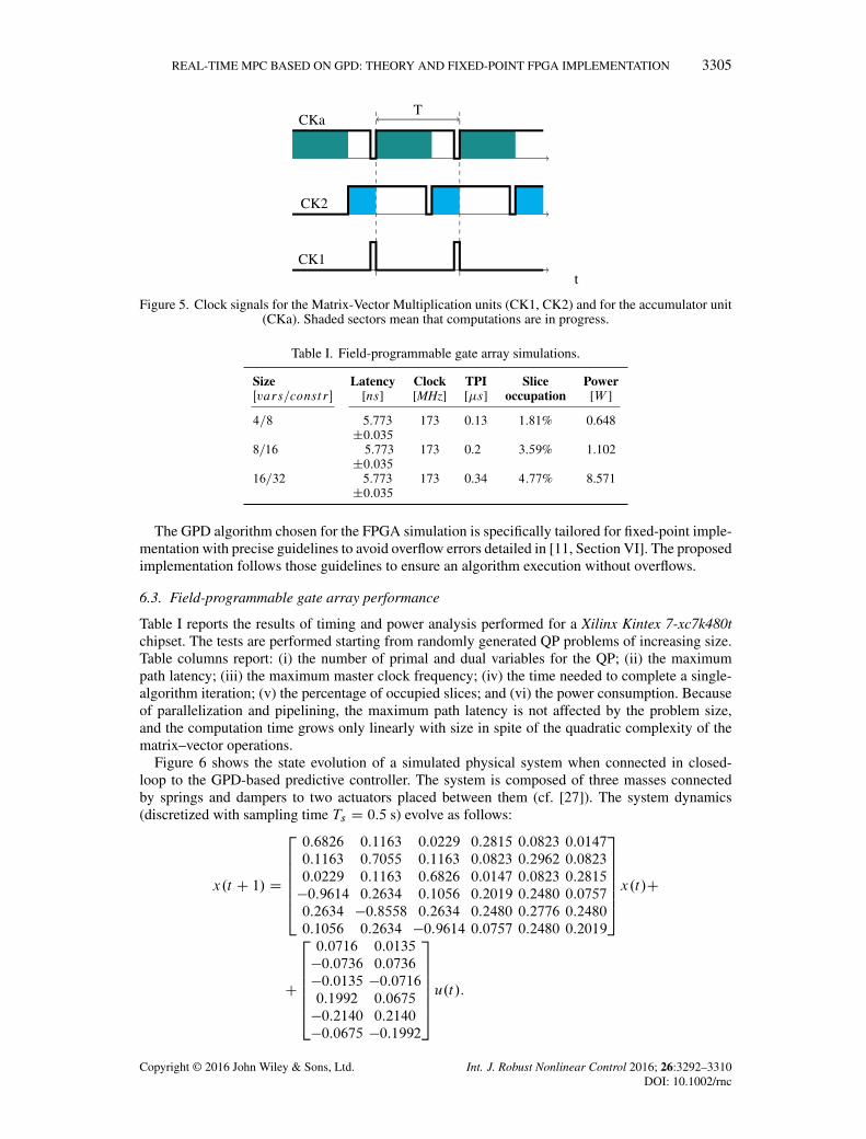
Figure 5. Clock signals for the Matrix-Vector Multiplication units (CK1, CK2) and for the accumulator unit(CKa). Shaded sectors mean that computations are in progress.

Table I. Field-programmable gate array simulations.

Size Latency Clock TPI Slice PowerŒvars=const r [ns] [MHz] [�s] occupation [W ]

4=8 5.773 173 0.13 1:81% 0.648˙0:035

8=16 5.773 173 0.2 3:59% 1.102˙0:035

16=32 5.773 173 0.34 4:77% 8.571˙0:035

The GPD algorithm chosen for the FPGA simulation is specifically tailored for fixed-point imple-mentation with precise guidelines to avoid overflow errors detailed in [11, Section VI]. The proposedimplementation follows those guidelines to ensure an algorithm execution without overflows.

6.3. Field-programmable gate array performance

Table I reports the results of timing and power analysis performed for a Xilinx Kintex 7-xc7k480tchipset. The tests are performed starting from randomly generated QP problems of increasing size.Table columns report: (i) the number of primal and dual variables for the QP; (ii) the maximumpath latency; (iii) the maximum master clock frequency; (iv) the time needed to complete a single-algorithm iteration; (v) the percentage of occupied slices; and (vi) the power consumption. Becauseof parallelization and pipelining, the maximum path latency is not affected by the problem size,and the computation time grows only linearly with size in spite of the quadratic complexity of thematrix–vector operations.

Figure 6 shows the state evolution of a simulated physical system when connected in closed-loop to the GPD-based predictive controller. The system is composed of three masses connectedby springs and dampers to two actuators placed between them (cf. [27]). The system dynamics(discretized with sampling time Ts D 0:5 s) evolve as follows:

x.t C 1/ D

2666664

0:6826 0:1163 0:0229 0:2815 0:0823 0:0147

0:1163 0:7055 0:1163 0:0823 0:2962 0:0823

0:0229 0:1163 0:6826 0:0147 0:0823 0:2815

�0:9614 0:2634 0:1056 0:2019 0:2480 0:0757

0:2634 �0:8558 0:2634 0:2480 0:2776 0:2480

0:1056 0:2634 �0:9614 0:0757 0:2480 0:2019

3777775 x.t/C

C

2666664

0:0716 0:0135

�0:0736 0:0736

�0:0135 �0:07160:1992 0:0675

�0:2140 0:2140

�0:0675 �0:1992

3777775u.t/:



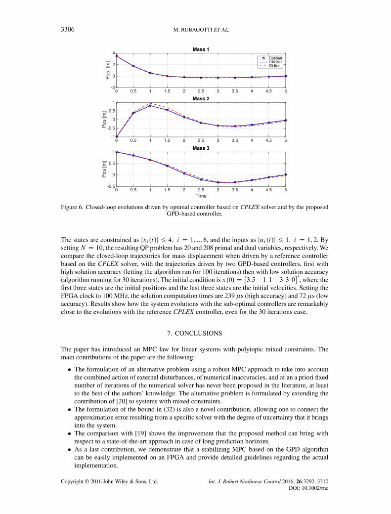
Figure 6. Closed-loop evolutions driven by optimal controller based on CPLEX solver and by the proposedGPD-based controller.

The states are constrained as jxi .t/j 6 4; i D 1; ::; 6, and the inputs as jui .t/j 6 1; i D 1; 2. BysettingN D 10, the resulting QP problem has 20 and 208 primal and dual variables, respectively. Wecompare the closed-loop trajectories for mass displacement when driven by a reference controllerbased on the CPLEX solver, with the trajectories driven by two GPD-based controllers, first withhigh solution accuracy (letting the algorithm run for 100 iterations) then with low solution accuracy(algorithm running for 30 iterations). The initial condition is x.0/ D

�3:5 �1 1 �3 3 0

�0, where the

first three states are the initial positions and the last three states are the initial velocities. Setting theFPGA clock to 100 MHz, the solution computation times are 239 �s (high accuracy) and 72 �s (lowaccuracy). Results show how the system evolutions with the sub-optimal controllers are remarkablyclose to the evolutions with the reference CPLEX controller, even for the 30 iterations case.

7. CONCLUSIONS

The paper has introduced an MPC law for linear systems with polytopic mixed constraints. Themain contributions of the paper are the following:

� The formulation of an alternative problem using a robust MPC approach to take into accountthe combined action of external disturbances, of numerical inaccuracies, and of an a priori fixednumber of iterations of the numerical solver has never been proposed in the literature, at leastto the best of the authors’ knowledge. The alternative problem is formulated by extending thecontribution of [20] to systems with mixed constraints.� The formulation of the bound in (32) is also a novel contribution, allowing one to connect the

approximation error resulting from a specific solver with the degree of uncertainty that it bringsinto the system.� The comparison with [19] shows the improvement that the proposed method can bring with

respect to a state-of-the-art approach in case of long prediction horizons.� As a last contribution, we demonstrate that a stabilizing MPC based on the GPD algorithm

can be easily implemented on an FPGA and provide detailed guidelines regarding the actualimplementation.



APPENDIX

A.1. Definitions regarding the asymptotic stability of a set

The following definitions are introduced in order to precisely describe the properties of the closed-loop system that are proved in Theorem 1. Consider a discrete-time autonomous nonlinear system

x.t C 1/ D '.x.t/; w.t//; (39)

where x 2 Rnx is the state vector, w 2 Rnw is the input vector, defined such that w.t/ 2 W (Wbeing a compact set including the origin), and '.�/ is a nonlinear function. The following definitions,adapted from [28], are recalled for the reader’s convenience. Consider two closed RPI sets OX andX , X � OX � Rnx . Then,

Definition 1 (attractivity)The set X is attractive for system (39), with domain of attraction OX , if, for all x.0/ 2 OX ,limt!1 ıh.x.t/;X / D 0.

Definition 2 (local stability)The set X is locally stable for system (39) if, for all 2 R>0, there exists ı 2 R>0 such that, foreach x.0/ satisfying x.0/ 2 X ˚Bı , one has x.t/ 2 X ˚B , for all t 2 N>0.

Definition 3 (asymptotic stability)The set X is asymptotically stable for system (39), with domain of attraction OX , if it is locally stableand attractive with domain of attraction OX .

A.2. Proof of Theorem 1

Part (1): We will first prove positive invariance of DN for (22), that is, if x 2 DN , then '.x/ 2 DN ,or, equivalently, SN .'.x// ¤ ; for every x 2 DN and every �.x/ 2 C.x/. Therefore, it is enoughto find a vector Qz 2 SN .'.x// for any x 2 DN , with Nz.x/ 2 Z.x/. Because x 2 DN , then theoptimal solution z? is such that

´?k D

�x?k

Kx?kC c?

k

�2 Zk; k 2 NN�1 (40)

and x?N 2 Xf �RN . Instead, for x 2 DN , we will be able to apply Nu0.x/ D Kx C �.x/ 2 C.x/,which will move the state to '.x/ D A�xCB�.x/ D A�xCBc?0 .x/Cw0, with w0 2W . In orderto determine a feasible solution Qz 2 SN .'.x//, we define the ‘shifted’ control vector

Qc.x/ D�Qc0.x/ : : : QcN�2.x/ QcN�1.x/

�D�c?1 .x/ : : : c

?N�1.x/ 0

�which defines Qz D

�Q 00 � � � Q

0N�1 Qx

0N

�0, with Qk D

�Qx0kK 0 Qx0

kC Qc0

k

�0, k 2 NŒ0;N�1�. We prove now

that Qz is a feasible solution for an initial state equal to '.x/. Applying the shifted control vectorQc.x/, we obtain

Qk D

�Qxk

K Qxk C Qck

�D ´?kC1 C

�I

K

�Ak�w0 (41)

From (40) and (41), one has, for k D 0; : : : ; N � 2,

Qk 2 ZkC1 ˚�I

K

�Ak�W D

�Z � QRkC1

�˚

�I

K

�Ak�W

D

��Z � QRk

��

�I

K

�Ak�W

�˚

�I

K

�Ak�W D

Zk �

�I

K

�Ak�W

�˚

�I

K

�Ak�W � Zk :



Again, by definition of Qc.x/, we have that QN�1 D�Qx0N�1 .K QxN�1/

0�0

, and by feasibil-ity of z?.x/ we know that x?N 2 Xf � AN� W � XN . By recalling Remark 2, we obtain´?N ,

�x?0N

�Kx?N

�0�02 ZN . Then, we can proceed as in (42), obtaining

QN�1 2 ZN ˚�I

K

�AN�1� W � ZN�1:

Finally, to prove that QxN 2 Xf �RN , we start investigating the properties of QxN�1:

QxN�1 2�Xf �RN

�˚ Ak�W D

h�Xf �RN�1

�� Ak�W

i˚ Ak�W � Xf �RN�1: (42)

Being Xf an RPI set with respect to dynamics (13), we know that, given x 2 Xf , Aj�x˚Rj � Xf ,or, equivalently, Aj�x 2 Xf � Rj , for all j 2 N>0 (remember that Xf � Rj ¤ ;, becauseR1 � Xf ). Therefore, given x 2 Xf � Rj�1, then A�x 2 Xf � Rj , for all j 2 N>1. Inconclusion, QxN�1 2 Xf � RN�1 implies QxN D A� QxN�1 2 Xf � RN . Recursive feasibility istherefore proved.

Part (ii): From the positive invariance of DN , being �.x.t// 2 C.x.t/// ¤ ;, one has.x.t/; �.x.t// 2 Z , for all t 2 N>0.

Part (iii): As a first step, we prove that for any initial condition x.0/ 2 DN , x.t/ converges toXf in a finite time. In order to do that, we consider the optimal value of the cost function VN .c/,evaluated at x.t/ and referred to as V ?N .t/ for the sake of readability. At time tC1, the existence of anew optimal value V ?N .t C 1/ for any realization of w.t/ 2W is guaranteed by recursive feasibility,but its explicit expression is not available. However, using the standard procedure used also in [20],we consider the suboptimal value of the cost function, corresponding to the shifted control sequenceQc.x.t//, that is,

QVN .t C 1/ D

N�1XkD0

Qc0k‰ Qck D

N�1XkD1

c?0k ‰c?k D V

?N .t/ � �

0t‰�t

where �t D c?0 .x.t//. We know that the optimal cost function at any x.tC1/ 2 A�x.t/CB�tCw.t/will be such that V ?N .tC1/ 6 QVN .tC1/, which implies V ?N .t/�V

?N .tC1/ > � 0t‰�t > 0. Therefore,®

V ?N .t/¯

is a non-negative non-increasing sequence, which converges to a finite value V ?N .1/ ast !1. If we consider the sum of the terms V ?N .t/ � V

?N .t C 1/, for t D 0; : : : ;1, we obtain

1 > V ?N .0/ � V?N .1/ >

1XtD0

� 0t‰�t > 0

which implies limt!1 �0t‰�t D 0, and, by positive definiteness of ‰, limt!1 �t D 0. Consider

now that, at any t 2 N>0, the uncertain term w.t/ is also applied to the system. Recalling that�.A�/ < 1,

limt!1

x.t/ D limt!1

"At�x.0/C

tXkD1

Ak�1� .B�t�k C w.t� k//

#D limt!1

"tX

kD1

Ak�1� w.t� k/

#2 R1:

Recalling Assumption 3, the asymptotic convergence of x.t/ to R1 implies that there exists Nt 2R>0 such that x.Nt / 2 Xf . Because Xf is a RPI set, by (21), the applied control law coincides with�.x/ (which in turn, coincides with the optimal control law) and then e.t/ D 0 for all t > Nt . From Nton, the system dynamics are therefore

x.t C 1/ D A�x.t/C d.t/ 2 Xf : (43)

As a consequence, the state converges asymptotically to the minimal RPI set for system (43), thatis RD in (15). Together with the finite-time convergence to Xf , this implies that the set RD isattractive for system (22) with domain of attraction DN , according to Definition 1.



In order to prove local stability, we consider the closed-loop dynamics (43) in Xf and take anyinitial condition x.0/ 2 RD ˚Bı . Being RD an RPI set for (43), we have that A�RD ˚D � RD ,and therefore, iterating the system dynamics

x.t/ 2 RD ˚ At�Bı : (44)

Being �.A�/ < 1, Definition 2 holds for the nominal system (5), the set X being the origin. Asa consequence, for all > 0, there exists ı > 0, such that At�Bı � B . By substituting thisinside (44), we conclude that x.t/ 2 RD ˚B , meaning that RD is locally stable for system (43),according to Definition 2, for any such that RD ˚B � Xf

In conclusion, Definition 3 holds for system (22), which proves that RD is asymptotically stablewith domain of attraction DN .

REFERENCES

1. Rawlings JB, Mayne DQ. Model Predictive Control: Theory and Design. Nob Hill Publishing: Madison, WI, 2009.2. Bemporad A, Morari M, Dua V, Pistikopoulos EN. The explicit linear quadratic regulator for constrained systems.

Automatica 2002; 38(1):3–20.3. Richter S, Jones CN, Morari M. Computational complexity certification for real-time MPC with input constraints

based on the fast gradient method. IEEE Transactions on Automatic Control 2012; 57(6):1391–1403.4. Nesterov Y. A method of solving a convex programming problem with convergence rate O.1=k2/. Soviet

Mathematics Doklady, Vol. 27, 1983; 372–376.5. Nesterov Y. Introductory Lectures on Convex Optimization: A Basic Course. Springer: New York City, NY, 2004.6. Necoara I, Suykens J. Application of a smoothing technique to decomposition in convex optimization. IEEE

Transactions on Automatic Control 2008; 53(11):2674–2679.7. Richter S, Morari M, Jones CN. Towards computational complexity certification for constrained MPC based on

Lagrange relaxation and the fast gradient method. Proceedings of the IEEE Conference on Decision and Control,Orlando, USA, 2011; 5223–5229.

8. Jerez JL, Goulart PJ, Richter S, Constantinides GA, Kerrigan EC, Morari M. Embedded predictive control on anFPGA using the fast gradient method. Proceedings of the European Control Conference, Zurich, Switzerland, 2013;3614–3620.

9. Patrinos P, Bemporad A. An accelerated dual gradient-projection algorithm for embedded linear model predictivecontrol. IEEE Transactions on Automatic Control 2014; 59(1):18–33.

10. Bemporad A, Patrinos P. Simple and certifiable quadratic programming algorithms for embedded linear model pre-dictive control. IFAC Conference on Nonlinear Model Predictive Control, Noordwijkerhout, Netherlands, 2012;14–20.

11. Patrinos P, Guiggiani A, Bemporad A. Fixed-point dual gradient projection for embedded model predictive control.Proceedings of the European Control Conference, Zurich, Switzerland, 2013; 3602–3607.

12. McGovern LK, Feron E. Closed-loop stability of systems driven by real-time, dynamic optimization algorithms.Proceedings of the IEEE Conference on Decision and Control, Phoenix, AZ, 1999; 3690–3696.

13. Giselsson P. Execution time certification for gradient-based optimization in model predictive control. IEEEConference on Decision and Control, Maui, HI, 2012; 3165–3170.

14. Necoara I, Ferranti L, Keviczky T. An adaptive constraint tightening approach to linear model predictive con-trol based on approximation algorithms for optimization. Optimal Control Applications and Methods 2015; 36(5):648–666.

15. Necoara I. Computational complexity certification for dual gradient method: application to embedded MPC. Systems& Control Letters 2015; 81:49–56.

16. Giselsson P, Boyd S. Preconditioning in fast dual gradient methods. IEEE Conference on Decision and Control, LosAngeles, CA, 2014; 5040–5045.

17. Doan MD, Keviczky T, De Schutter B. A distributed optimization-based approach for hierarchical MPC of large-scale systems with coupled dynamics and constraint. IEEE Conference on Decision and Control, Orlando, FL, 2011;5236–5241.

18. Necoara I, Nedelcu V. Rate analysis of inexact dual first-order methods: application to dual decomposition. IEEETransactions on Automatic Control 2014; 59(5):1232–1243.

19. Rubagotti M, Patrinos P, Bemporad A. Stabilizing linear model predictive control under inexact numericaloptimization. IEEE Transactions on Automatic Control 2014; 59(6):1660–1666.

20. Chisci L, Rossiter JA, Zappa G. Systems with persistent disturbances: predictive control with restricted constraints.Automatica 2001; 37(7):1019–1028.

21. Rakovic SV, Kerrigan EC, Kouramas KI, Mayne DQ. Invariant approximations of the minimal robust positivelyinvariant set. IEEE Transactions on Automatic Control 2005; 50(3):406–410.

22. Bertsekas DP, Nedic A, Ozdaglar AE. Convex analysis and optimization. Athena Scientific: Nashua, NH, 2003.23. Jerez JL, Goulart PJ, Richter S, Constantinides GA, Kerrigan EC, Morari M. Embedded online optimization for

model predictive control at megahertz rates. IEEE Transactions on Automatic Control 2014; 59(12):3238–3251.



24. Jerez JL, Constantinides GA, Kerrigan EC. An FPGA implementation of a sparse quadratic programming solver forconstrained predictive control. Proceedings of the ACM/SIGDA International Symposium on Field ProgrammableGate Arrays, Monterey, CA, 2011; 209–218.

25. Wills AG, Knagge G, Ninness B. Fast linear model predictive control via custom integrated circuit architecture. IEEETransactions on Control Systems Technology 2012; 20(1):59–71.

26. Kerrigan EC, Jerez JL, Longo S, Constantinides GA. Number representation in predictive control. Proceedings of theIFAC Conference on Nonlinear Model Predictive Control, Noordwijkerhout, Netherlands, 2012; 60–67.

27. Wang Y, Boyd S. Fast model predictive control using online optimization. IEEE Transactions on Control SystemsTechnology 2010; 18(2):267–278.

28. Rawlings JB, Mayne DQ. Postface to Model Predictive Control: Theory and Design, 2011. (Available from: http://jbrwww.che.wisc.edu/home/jbraw/mpc/postface.pdf) [accessed on 19 August 2012].


http://jbrwww.che.wisc.edu/home/jbraw/mpc/postface.pdf

http://jbrwww.che.wisc.edu/home/jbraw/mpc/postface.pdf

real-time model predictive control based on dual...

Documents