P a g e | 1

Genetic Phase Angle Distance (GPAD)

Daniel K. Pratt

B.S. Biotechnology, Utah Valley University, Orem, UT

April 2013

Abstract

It is hypothesized that a mapping of the biochemical properties of genetic nucleotides

into the three dimensional ℝ3 Clifford algebra will yield a novel and meaningful evolutionary

distance measure. The nucleotides A,T,C,G are mapped according to three biochemical

properties (amino/keto, purine/pyrimidine, weak/strong), resulting in four base-vectors. A

weighted linear combination of the base-vectors as codon triplets results in a "Tetrahedral

Genetic Code" (TGC), where all 64 codons map to 64 unique codon-vectors in the space. Phase

distance θ is measured as the angle between sequentially neighboring codon-vectors, and a

sequence of codons is measured as the total path length in radians of the vector as it traverses the

TGC. Angular difference Δθ is computed as the absolute value of the difference in phase θ

between sequences, at homologous loci. The Genetic Phase Angle Distance (GPAD) is computed

as the Δθ mean. GPAD is computed on a sample sequence matrix for 11 different species and

compared side by side to the Equal-input distance and phylogenetic tree computed on that same

species matrix.

Table of Contents

I. Introduction ……………………………………………………….2 II. An Imaginary Science ………………………………………..3 III. The Mathematics of Complex Signals .……………………….5 IV. Computational Framework ………………………………………..6 V. Experimental Setup and Results ………………………………..10 VI. Discussion/Conclusion .……………………………………….13

References ..………………………………………………………16 Appendix A – Additional Figures ..………………………………18 Appendix B – Explicit Mathematica computational code ...……...19

P a g e | 2

I. Introduction

There has been a growing discontent in the fringes of the Biosciences concerning the

erroneous emphasis of its methodologies upon the discrete information contained within the

genome. There is call for a more explicit study of the different kinds of representations that can

exist in biology vis-a-vis complex dynamical systems. Beyond the observables known from

physics, there is a need for new observables in biology that will increase its intelligibility and

facilitate the quantification of collective biological organization. (Bailly & Longo, 2009; Longo,

Miquel, Sonnenschein, & Soto, 2012; Rocha & Hordijk; Simeonov, 2010) In this paper I will

present a novel method of deriving molecular evolutionary distances via a three dimensional

representation of the genetic code, and argue the validity of a unique subjective ontology which

might be observed at the level of molecular biology.

Over the past decade, a number of new methods of genomic analysis have been introduced. The

fractal properties of DNA (Cattani, 2010), the ability to generate linguistic statements from its

codons (Lee et al., 2011), and the application of quantum algorithms to the genetic code

(Patel, 2001; Rieper, Anders, & Vedral, 2010) emphasize the interactions between molecules,

rather than treating a single base as an individual unit of information. Current evidence

indicates that genomes are complex landscapes defined by physical structures and forces of

extremely long range which can appropriately be considered another level of genetic coding.

(Mauger, Siegfried, & Weeks, 2013; Melkikh, 2013) In particular, genomic signal processing

(Chheda, 2012) involves a reconceptualization of biological information, as much as it offers

new and interesting methods of accessing its content. The signal analytic genomic model and

measure presented in this work are called the Tetrahedral Genetic Code (TGC) and Genetic

Phase Angle Distance (GPAD), respectively.

P a g e | 3

II. An Imaginary Science

To begin, it must be acknowledged that the established methods of molecular biology,

and specifically the genetic code, are practically irrefutable. Nevertheless, while the triplet

genetic code is the most common lookup table used to decode genomic information, the elegance

of the three letter genetic code has often focused analysis of the human genome on the sequence

of nucleotides, neglecting the possibility of additional codes in the genome both within and

outside the coding regions. (Parker & Tullius, 2011; Robins, Krasnitz, & Levine, 2008) This can

be compared to the dangerously misleading ball-and-stick models of chemistry, with which we

tend to assume that the actual bonding phenomenon is concentrated along those very lines. A

molecule is not a hard and rigid object, but rather, a dense bundle of energy characterized by

smoothness and dynamics. (Hyde, 1997) Similarly, the cell is not a computer, indifferent to the

sequence data it processes. The genome is fundamentally different: its states depend upon its

knowledge content. (Stern, 2000)

A simple and effective way to gain insight into the collective nature of biological

information is to extend it metaphorically into more recent models of physics and the

mathematics of complexity. Whereas in physics we may wonder, “can one hear the shape of a

drum?” (Kac, 1966), in biology we might ask if the cell can “hear” the shape of a protein. In

(Brown, 1972), we are reminded that a mathematical description of cellular activity might be

compared with a practical art form like cookery, in which the taste of a cake (protein shape),

although literally indescribable, can be conveyed to a reader in the form of a set of injunctions

called a recipe (an amino acid sequence). In both cases, we arrive at a qualitative, rather than

quantitative, description which is characteristic of systems thinking – from objects to

relationships. (Capra, 1996)

P a g e | 4

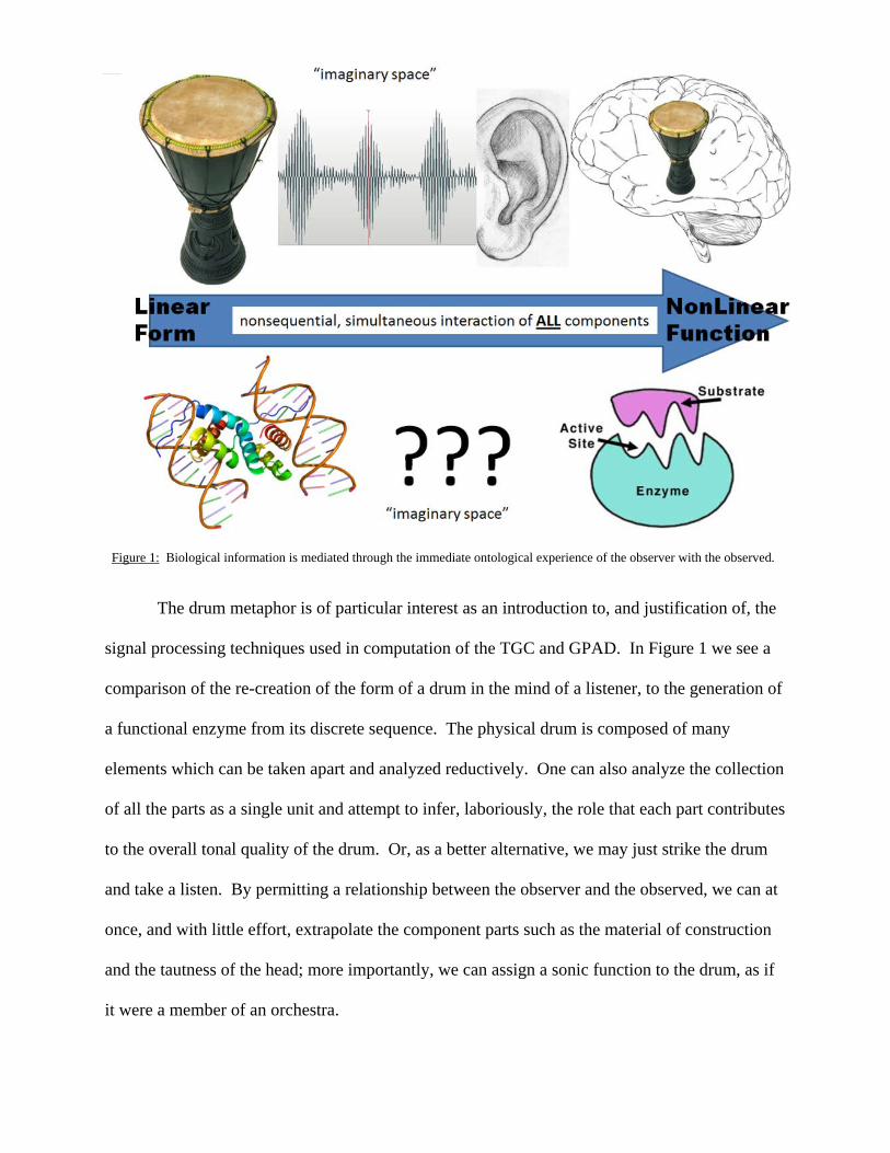
The drum metaphor is of particular interest as an introduction to, and justification of, the

signal processing techniques used in computation of the TGC and GPAD. In Figure 1 we see a

comparison of the re-creation of the form of a drum in the mind of a listener, to the generation of

a functional enzyme from its discrete sequence. The physical drum is composed of many

elements which can be taken apart and analyzed reductively. One can also analyze the collection

of all the parts as a single unit and attempt to infer, laboriously, the role that each part contributes

to the overall tonal quality of the drum. Or, as a better alternative, we may just strike the drum

and take a listen. By permitting a relationship between the observer and the observed, we can at

once, and with little effort, extrapolate the component parts such as the material of construction

and the tautness of the head; more importantly, we can assign a sonic function to the drum, as if

it were a member of an orchestra.

Figure 1: Biological information is mediated through the immediate ontological experience of the observer with the observed.

P a g e | 5

Considering these two methods of drum analysis, we can see immediately that an attempt

to understand the function of the drum from a reductionist point of view is futile. Even if we

manage, by some major effort, to model the drum as a collection (of parts), we will gain very

little knowledge of its timbre. Likewise, it is common knowledge that the derivation of protein

shape via amino acid sequence is nearly intractable. It is tempting to consider that there might

exist some mediator of protein from form to function as a direct, subjective, sensational

experience. That the cellular environment and molecular structures are capable of supporting

this type of behavior through a quantum interpretation of biology is becoming increasingly

supported in the literature. (Plankar, Brežan, & Jerman, 2013; Rieper et al., 2010; Rowlands,

2007) How to mold the measure of a molecular “experience” into the form of a science is the

central question in the transition from bioinformatics to biosemiotics.

III. The Mathematics of Complex Signals

The mathematics of complexity is one of relationships and patterns. Complexity in the

natural world is manifested through implicit and explicit order. The implicit order can be

encoded in ‘hidden variables’ that enable semantic enfolding and unfolding in the formal world.

(Bohm, 1952) Looking again at Figure 1, the physical drum is explicit, its mental recreation is

implicit, and the “encoded hidden variables” are represented by the complex waveform that lies

between them.

In terms of genomics, the distinguishing biochemical properties of DNA nucleotides can

encode three overlapping modes of discrete computation simultaneously: each nucleotide can be

described as a purine or pyrimidine, as containing an amino or keto group, and by having either

two or three hydrogen bond pairings with its complimentary base. Thus the explicit order, a

single structural change within a DNA strand, can be described by three different characteristics

P a g e | 6

at once. It is through the formal superposition of these variables in an abstract mathematical

space called a "phase space", that we hope to find, in the experiment to follow, an implicit order

of the genetic sequences. The three nucleotide characteristics are represented by independent

coordinates in three dimensions of the phase space. Thus, a single point in the space describes

the simultaneous state (“taste”) of the entire system. (Capra, 1996) In this way, we transform the

genetic sequence into a signal like unto the complex sonic waveform of the drum. From there,

we may treat the waveform via a plethora of computational techniques which have already been

used extensively and with significant success in bioinformatics, including such tools as hidden

Markov models and neural networks, the discrete Fourier transform (DFT), FIR digital filtering,

wavelets, and spectrograms. (Anastassiou, 2001) The techniques used in the computation of the

TGC and GPAD are founded upon the work of (Cristea, 2005). Similar analytical methods can

be found in (Brodzik & Peters, 2005), the dyadic and Hadamard genomatrices of (Petoukhov,

2010), and in (Rowlands, 2007) genetic formulation of the Dirac nilpotent algebra.

IV. Computational Framework

The tetrahedral genetic code (TGC) was computed and rendered using the Mathematica

package 'clifford.m' which implements general operations of a Clifford algebra on the language

of the computer algebra program Mathematica, and has been enriched with functions to draw

multivectors in ℝ3. (Aragon-Camarasa, Aragon-Gonzalez, Aragon, & Rodriguez-Andrade, 2008)

The package 'clifford.m', a user guide, a palette with the most common predefined functions, the

notebook with the calculations by (Zhang, Zhu, Peng, & Chen, 2006), as well as the explicit

Mathematica code for all calculations in this experiment are available for download (see

Appendix B).

P a g e | 7

A vector has a length (scalar value) and direction, which we can represent as a directed

line segment in 3D; it can stem from the origin of a Euclidean coordinates system and move to a

point in three dimensions. Geometric algebra has four basic computing elements in 3D physical

space: scalar, vector, bivector, and trivector. Linear compositions of geometric algebra’s basic

computing elements are called multivectors, and are denoted by uppercase Latin letters, such as

A, B, and C. We use the term k-vector to denote a k-dimensional subspace, which is formed

from the outer product of vectors. For any k-vector Ak, when k = 0, 1, 2, or 3, Ak represents a

scalar, vector, bivector, or trivector, respectively. (Zhang et al., 2006)

Nucleotide and Codon Mappings

All elements of the TGC will be represented by 1-vectors: A1 , T1 , G1 , C1; where each

symbol is the first letter of the respective genetic nucleotide Adenine, Thymine, Guanine, or

Cytosine. In Mathematica code, we denote the j-th basis vector as ej. Accordingly, the ℝ3

geometric algebra basis vectors are e1, e2, and e3. The four nucleotides are mapped as:

A1 = e1 +e2 +e3 T1 = e1 −e2 −e3 G1 = −e1 −e2 +e3 C1 = −e1 +e2−e3

Figure 2: Nucleotides are mapped into a complex vector space, as represented in Mathematica using ‘clifford.m’ (Aragon, 2008).

P a g e | 8

The sign values play the important role of distinguishing the three specific biochemical

characteristics (one on each axis) associated with each nucleotide. For e1, a positive sign

indicates that the base has a ‘weak’ 2-hydrogen bond pairing with its compliment in the opposite

strand; a negative sign indicates a ‘strong’ 3-hydrogen bond pairing. Similarly along e2, positive

values indicate a nucleotide with an amino group and negative values give a nucleotide with a

keto group. Finally, in e3 the positive and negative signs represent the purines and pyrimidines,

respectively. The nucleotide 3-D mappings are visualized in Figure 2.

The mapping of a codon from the standard genetic code into the vector space is

accomplished as a weighted, linear combination of its three vector nucleotide components,

resulting in a composite vector. Given a protein-coding sequence, each codon is decomposed

into its first, second and third elements; the first nucleotide is denoted by α, the second by β, and

the third by γ. Following, each vector is given a multiplicative weighting factor according to its

relative importance (due to degeneracy) in determining the codon’s resultant amino acid. Given

a sequence containing N number of codon triplets, the codon-vector sequence is defined as

δn({{αn,βn,γn},{…},{αN,βN,γN}}) {{4αn + 2βn + γn},{…},{4αN + 2βN + γN}},

(n = 1, 2, …., N; α, β, γ ∈ {A1 ,T1 ,G1 ,C1})

An ordered mapping of all 64 genetic codons into the vector space yields 64 unique

vectors, and is visualized as tetrahedral in shape. Taken all at once, the genetic code, mapped as

the TGC, is shown in Figure 3. The tetrahedral representation expresses the symmetry and

degeneration of the genetic code; generates mappings of nucleotide, codon and amino acid

sequences into genomic signals; and translates multiple modes of biochemical properties into a

single, simultaneous, signal property. Codons corresponding to the same amino acid are mapped

to neighboring points within the tetrahedron, i.e., related codons are clustered. The complex

P a g e | 9

mappings cluster the multiple

representations of the same amino acid in

contiguous regions of the space. (Cristea,

2003)

Genetic Phase Angle Distance

For any two consecutive codon-

vectors, δi ({αi, βi, γi}) and δj ({αj, βj, γj}),

let θ(𝑖 ,𝑗) be the angle between them. For

N=64 unique elements of the TGC, there

exist 642

2 possible θ(𝑖 ,𝑗). The two-

dimensional matrix of all ordered

combinations between pairs of codon-vectors is

a finite field of θ(NxN). If each position of the

resulting matrix is assigned a color and intensity

requisite to the value of its measured angle, a

fractal-like pattern with interesting symmetries

emerges (Figure 4).

Any given protein-coding sequence can

be plotted linearly as a path within the finite

θ(NxN) matrix; or more simply, a genetic

sequence mapped into the TGC is the smooth

path on the surface of a sphere which is drawn

Figure 3: 64 codons map to 64 unique vector positions resulting in a tetrahedral genetic code.

Figure 4: A matrix of all possible values of θ (small θlight, large θdark).

P a g e | 10

as a result of a vector traversing the sequential codon-vector positions. This sequential path of

angles is then transferred to a Cartesian plot with phase angle (in radians) on the y-axis and time

(in arbitrary units) on the x-axis. The θ sequence paths of the first exon of the β-globin gene for

the two species Human and Gallus is shown in Figure 5. Also shown in the figure is the

immediate precursor of the Genetic

Phase Angle Distance (GPAD)

measure, Δθ, defined as the absolute

value of the difference between the

two sequence paths. This measure

will be used in the following section

in an attempt to derive evolutionary

distances between a number of

distantly related species.

V. Experimental Setup and Results

An initial test of the validity of the GPAD was conducted by taking the measure over a

sample set of genetic sequences, and making a direct comparison to an established distance

measure over that same sample set. The sequences for the β-subunit of hemoglobin for eleven

different species were located using (Jafarzadeh & Iranmanesh, 2013), and confirmed by BLAST

(Altschul, 1997). The curated sequences were then imported into the MEGA5 software (Tamura

et al., 2011) and an alignment was performed using the MUSCLE algorithm (Edgar, 2004). It

should be noted that a major drawback of the current GPAD computational framework is the

inability to properly handle indel mutations. Because the framework is set up as a direct

mapping from pairs of codon-vectors to their corresponding angle measure, any gap-containing

Figure 5: θ and Δθ sequence plots of the first exon of the β-globin gene for Human and Gallus.

P a g e | 11

alignment (example: {A,-,G}) will not receive coordinates in the vector space. Rather, gap-

containing triplets are mapped to the origin (zero). For this reason, the sequence and alignment

parameters were selected with the primary goal of limiting the effect of indel mutations. Table 1

(Appendix A) gives the eleven aligned β-globin sequences under examination.

The procedure for transformation of the eleven genetic sequences into TGC θ and Δθ

sequence paths was performed as outlined in the previous section, resulting in an (ixjxk) matrix

where i and j represent the ordered combinations of all species in the sample set, and k is the Δθ

sequence between the ith and jth species. The (ixjxk) matrix is then reduced to (ixj) by taking the

mean angular distance within each Δθ path, resulting in a single value at every position of the

square matrix. This final procedure is formalized, and an example given, in Figure 6.

The GPAD matrix was compared to a set of sixteen standardized distance measures by

taking the difference of matrices 𝟐𝑵𝟐

∑∑ �𝒂(𝒊,𝒋)−𝒃(𝒊,𝒋)�, resulting in a measure of variance between

them. Table 2 gives the results of this similarity test, revealing a significant match between

GPAD and the ‘Equal-input’ model (Tamura et al., 2011). The GPAD matrix for all eleven

species, along with a representation of

its values according to relative color

and intensity, is shown in the upper

section of Figure 7. For direct

comparison, a second matrix was

constructed with the same aligned

sequences using the Equal input model,

shown in the lower half of the figure.

Figure 6: GPAD is calculated as the normalized mean Δθ between two homologous protein-coding sequences.

P a g e | 12

A second experiment was conducted in order to

further explore the similarity between the GPAD and

Equal-input models. The mean θ sequence path between

all eleven species, and the Δθ and GPAD of each species

sequence against that mean were computed. A

phylogenetic tree, rooted to Gallus, was computed on the

species matrix using the following settings: UPGMA,

Equal-input model, neighbor-joining, bootstrap

replications: 500, uniform rates among sites. These

additional GPAD-distance-from-mean values and

phylogenetic analysis are shown in Figure 8.

Figure 7: Side by side comparison of sequences from Table XX using distance measures: GPAD (upper) and Equal input model (lower).

Table 2: difference of matrices between GPAD and sixteen standardized distance measures.

P a g e | 13

VI. Discussion/Conclusion

The Tetrahedral Genetic Code is a projection of multiple modes of nucleotide

biochemical information into a complex phase space, represented by the ℝ3 Clifford geometric

algebra. A genetic sequence of triplet codons mapped into this space can be thought of as the

path on the surface of a sphere correlating to the motion of angular transitions between

consecutive codon-vectors. Any two homologous coding sequences can plotted as a function of

angular distance (radians) in time, and the positive difference between their paths is interpreted

as a distance of molecular evolution. The GPAD is the mean score of this difference.

It is difficult to quantify the accuracy and utility of the GPAD due to the small size of the

experimental sample set and sequence length. Nevertheless, even a quick subjective assessment

of the results leaves little doubt that GPAD is at least as effective a measure of evolutionary

distance as many of the distance measures currently in regular use. The figure with the colored

matrices shows quite plainly that the two data sets follow the same overall trend; and closer

inspection of the numerical values reveals that in many cases, those values are in the same

neighborhood. As noted in Table 2, the average variance between the two matrices in the figure

is 0.1, meaning that the two measures are indeed quite similar. Also of note in that table is the

segregation of amino-acid and nucleotide substitution models, with amino-acid substitution

faring better in all cases. It is supposed that this is due to the fact that GPAD is also based to

some degree on amino-acid substitution.

The phylogenetic analysis in Figure 8 shows the peculiar correspondence of the Equal-

input lineage to the increasing order of species GPAD-distance-from-mean scores. As shown in

better detail in Figure 9 (Appendix A), the mean θ path most closely resembles the most recent

sequence, human, while the most distant sequence, opossum, has the widest variation from the

P a g e | 14

mean. Other than the interchange of the goat/bovine and mouse/rat branches, the two lists fall

into an identical ordering. This additional information lends support to the similarity of GPAD

to the Equal-input model. However, because the distance-from-mean approach is an atypical

assessment of inheritance, it is unclear if the similarity in ordering is coincidental, if it is also

observed in the standard models, or if it is detecting some central tendency or attraction via the

mechanisms of evolution toward some ‘optimal’ amino-acid sequence, represented by the mean

θ path. It will be interesting to see, in future study, if the GPAD-distance-from-mean continues

to exhibit this unexpected property.

Figure 8: A table of GPAD-distance-from-mean scores, compared to phylogenetic analysis (boostrap consensus values at branch points).

P a g e | 15

What is particularly interesting about the mean θ path is that it does not represent some

explicit genetic sequence, but rather, it represents a relative configuration of the relationships

between codons. In other words, for any given path, there exist many codon sequences that will

satisfy its angular distance relationships. There is no stipulation in the GPAD for origination or

direction of travel through the three dimensional vector space: its only measure is angle. It is

noted, however, that the vector magnitude and direction of travel are possible avenues for further

study. It may also be interesting to assess the θ and Δθ paths in comparison to protein domains,

to perhaps uncover new clues about the nature of protein folding.

Because of the ambiguous, non-directional, property of the θ path, a useful metaphor is

that the path is like unto a musical melody, wherein the relative frequencies between neighboring

notes is important, but not the absolute values of the frequencies of individual notes: the melody

is recognized irrespective of the key in which it is reproduced. (Petoukhov, 2010) The process of

“recognition” of an in-tune or out-of-tune molecular sequence or conformation is a good

candidate for the emergence of the “self” in self-replication, via the coarse-graining of phase

space. (England, 2012) Indeed, the Tetrahedral Genetic Code and Genetic Phase Angle Distance

could be an important step in the development of a statistical method reminiscent of quantum

mechanics, helping to uncover why nonsynonymous sequences can assume very similar

functional shapes and domains (Parker, 2011), and why changing the nucleotides in the third

position of codons in regulatory elements increases the rate of transcription of these elements

many fold (Robins et al., 2008; Subramaniam, Pan, & Cluzel, 2013), among the many

outstanding problems of molecular biology.

P a g e | 16

References Altschul, S. (1997). Gapped BLAST and PSI-BLAST: a new generation of protein database

search programs. Nucleic Acids Research, 25(17), 3389–3402. doi:10.1093/nar/25.17.3389 Anastassiou, D. (2001). Genomic signal processing. IEEE Signal Processing Magazine, 18(4),

8–20. doi:10.1109/79.939833 Aragon-Camarasa, G., Aragon-Gonzalez, G., Aragon, J. L., & Rodriguez-Andrade, M. A.

(2008). Clifford Algebra with Mathematica. Retrieved from http://arxiv.org/pdf/0810.2412 Bailly, F., & Longo, G. (2009). Biological Organization and Anti-entropy. Journal of Biological

Systems, 17(01), 63–96. doi:10.1142/S0218339009002715 Bohm, D. (1952). A Suggested Interpretation of the Quantum Theory in Terms of "Hidden"

Variables. I. Physical Review, 85(2), 166–179. doi:10.1103/PhysRev.85.166 Brodzik, A., & Peters, O. (2005). Symbol-balanced quaternionic periodicity transform for latent

pattern detection in DNA sequences. Acoustics, Speech, and Signal Processing, 2005. Proceedings. (ICASSP '05). IEEE International Conference on, 373–376. doi:10.1109/ICASSP.2005.1416318

Brown, G. S. (1972). Laws of form (Limited ed.). New York: Julian Press. Capra, F. (1996). The web of life: A new scientific understanding of living systems. United States:

DOUBLEDAY (NY/MD). Cattani, C. (2010). Fractals and Hidden Symmetries in DNA. Mathematical Problems in

Engineering, 2010(12), 1–32. doi:10.1155/2010/507056 Chheda, N., Turakhia, N., Gupta, M. K., Shah, R., & Raisinghani, J. (2012). Biospectrogram: a

tool for spectral analysis of biological sequences. arXiv:1210.1472v1 [q-bio.QM] Cristea, P. D. (2003). Large scale features in DNA genomic signals. Signal Processing, 83(4),

871–888. doi:10.1016/S0165-1684(02)00477-2 Cristea, P. D. (2005). Representation and analysis of DNA sequences. In E. R. Dougherty (Ed.),

EURASIP book series on signal processing and communications v. 2. Genomic signal processing and statistics. New York, N.Y: Hindawi Pub. Corp.

Edgar, R. C. (2004). MUSCLE: multiple sequence alignment with high accuracy and high throughput. Nucleic acids research, 32(5), 1792–1797. doi:10.1093/nar/gkh340

England, J. L. (2012). Statistical Physics of Self-Replication. arXiv:1209.1179v1 [physics.bio-ph]

Hyde, S. (1997). The language of shape: The role of curvature in condensed matter: physics, chemistry and biology. Amsterdam ; Oxford: Elsevier.

Jafarzadeh, N., & Iranmanesh, A. (2013). C-curve: A novel 3D graphical representation of DNA sequence based on codons. Mathematical Biosciences, 241(2), 217–224. doi:10.1016/j.mbs.2012.11.009

Kac, M. (1966). Can One Hear the Shape of a Drum? The American Mathematical Monthly, 73(4), 1. doi:10.2307/2313748

Lee, J.-H., Lee, S. H., Chung, W.-H., Lee, E. S., Park, T. H., Deaton, R., & Zhang, B.-T. (2011). A DNA assembly model of sentence generation. Biosystems, 106(1), 51–56. doi:10.1016/j.biosystems.2011.06.007

P a g e | 17

Longo, G., Miquel, P.-A., Sonnenschein, C., & Soto, A. (2012). Is information a proper observable for biological organization? Progress in Biophysics and Molecular Biology, 109(3), 108–114. doi:10.1016/j.pbiomolbio.2012.06.004

Mauger, D. M., Siegfried, N. A., & Weeks, K. M. (2013). The genetic code as expressed through relationships between mRNA structure and protein function. FEBS Letters, 587(8), 1180–1188. doi:10.1016/j.febslet.2013.03.002

Melkikh, A. V. (2013). Biological complexity, quantum coherent states and the problem of efficient transmission of information inside a cell. Biosystems, 111(3), 190–198. doi:10.1016/j.biosystems.2013.02.005

Parker, S. C. J., & Tullius, T. D. (2011). DNA shape, genetic codes, and evolution. Current Opinion in Structural Biology, 21(3), 342–347. doi:10.1016/j.sbi.2011.03.002

Patel, A. (2001). Quantum Algorithms and the Genetic Code. arXiv:quant-ph/0002037v3 Petoukhov, S. V. (2010). Matrix genetics, part 5: genetic projection operators and direct sums.

Retrieved from http://arxiv.org/pdf/1005.5101 Plankar, M., Brežan, S., & Jerman, I. (2013). The principle of coherence in multi-level brain

information processing. Progress in Biophysics and Molecular Biology, 111(1), 8–29. doi:10.1016/j.pbiomolbio.2012.08.006

Rieper, E., Anders, J., & Vedral, V. (2010). Quantum entanglement between the electron clouds of nucleic acids in DNA. Retrieved from http://arxiv.org/pdf/1006.4053

Robins, H., Krasnitz, M., & Levine, A. J. (2008). The Computational Detection of Functional Nucleotide Sequence Motifs in the Coding Regions of Organisms. Experimental Biology and Medicine, 233(6), 665–673. doi:10.3181/0704-MR-97

Rocha, L. M., & Hordijk, W. From the Genetic Code to the Evolution of Cellular Automata. Artificial Life XI: Eleventh International Conference on the Simulation and Synthesis of Living Systems, 11(1-2), 189–214.

Rowlands, P. (2007). Zero to infinity: The foundations of physics (Vol. 41). New Jersey: World Scientific.

Simeonov, P. L. (2010). Integral biomathics: A post-Newtonian view into the logos of bios. Progress in Biophysics and Molecular Biology, 102(2-3), 85–121. doi:10.1016/j.pbiomolbio.2010.01.005

Stern, A. (2000). Quantum Theoretic Machines: What is thought from the point of view of physics. Amsterdam: North-Holland; Elsevier Science.

Subramaniam, A. R., Pan, T., & Cluzel, P. (2013). Environmental perturbations lift the degeneracy of the genetic code to regulate protein levels in bacteria. Proceedings of the National Academy of Sciences, 110(6), 2419–2424. doi:10.1073/pnas.1211077110

Tamura, K., Peterson, D., Peterson, N., Stecher, G., Nei, M., & Kumar, S. (2011). MEGA5: molecular evolutionary genetics analysis using maximum likelihood, evolutionary distance, and maximum parsimony methods. Molecular biology and evolution, 28(10), 2731–2739. doi:10.1093/molbev/msr121

Zhang, H., Zhu, C., Peng, Q., & Chen, J. (2006). Using geometric algebra for 3D linear transformations. Computing in Science & Engineering, 8(3), 68–75. doi:10.1109/MCSE.2006.54

P a g e | 18

Appendix A – Additional Figures

Tabl

e 1:

The

cod

ing

sequ

ence

s of t

he fi

rst e

xon

of B

-glo

bin

gene

in 1

1 di

ffer

ent s

peci

es, a

ligne

d by

cod

on h

omol

ogy

usin

g M

USC

LE {

Edga

r 200

4 #1

33}.

Figu

re 9

: th

e θ

path

s of m

axim

um a

nd m

inim

um v

aria

nce

from

the

mea

n θ

path

.

P a g e | 19

Appendix B – Explicit Mathematica computational code

This code is also available as a Mathematica notebook file in the supplemental materials located at: https://docs.google.com/file/d/0Bzgyyvz44CkRUkx1aVRqNTZxVTA/edit?usp=sharing

(* !!! push 'shift-enter' to execute the notebook !!! *) (*import the clifford algebra package clifford.m; available for download http://www.fata.unam.mx/aragon/software*) <<clifford.m (*computation: map nucleotides into 3D vector space*) {a=Distribute[e[1]+e[2]+e[3]],c=Distribute[-e[1]+e[2]-e[3]],g=Distribute[-e[1]-e[2]+e[3]],t=Distribute[e[1]-e[2]-e[3]]}; (*graphic: vector-codons*) {"A",GADraw[a],"T",GADraw[t],"G",GADraw[g],"C",GADraw[c]} (*graphic: 3D plot of Tetrahedral Genetic Code*) {{AAA=Distribute[Simplify[4a+2a+a]],AAT=AAT=Distribute[Simplify[4a+2a]]+t,AAC=Distribute[Simplify[4a+2a+c]],AAG=Distribute[Simplify[4a+2a+g]]},{ATA=Distribute[Simplify[4a+a]]+Distribute[2t],ATT=Distribute[Simplify[4a+2t+t]],ATC=Distribute[Simplify[4a+2t+c]],ATG=Distribute[Simplify[4a+2t+g]]},{ACA=Distribute[Simplify[4a+2c+a]],ACT=Distribute[Simplify[4a+2c+t]],ACC=Distribute[Simplify[4a+2c+c]],ACG=Distribute[Simplify[4a+2c+g]]},{AGA=Distribute[Simplify[4a+2g+a]],AGT=Distribute[Simplify[4a+2g+t]],AGC=Distribute[Simplify[4a+2g+c]],AGG=Distribute[Simplify[4a+2g+g]]},{TAA=Distribute[Simplify[4t+2a+a]],TAT=Distribute[4t]+Distribute[2a]+Distribute[t],TAC=Distribute[Simplify[4t+2a+c]],TAG=Distribute[Simplify[4t+2a+g]]},{TTA=Distribute[4t]+Distribute[2t]+Distribute[a],TTT=Distribute[Simplify[4t+2t+t]],TTC=Distribute[Simplify[4t+2t+c]],TTG=Distribute[Simplify[4t+2t+g]]},{TCA=Distribute[Simplify[4t+2c+a]],TCT=Distribute[Simplify[4t+2c+t]],TCC=Distribute[Simplify[4t+2c+c]],TCG=Distribute[Simplify[4t+2c+g]]},{TGA=Distribute[Simplify[4t+2g+a]],TGT=Distribute[Simplify[4t+2g+t]],TGC=Distribute[Simplify[4t+2g+c]],TGG=Distribute[Simplify[4t+2g+g]]},{CAA=Distribute[Simplify[4c+2a+a]],CAT=Distribute[Simplify[4c+2a+t]],CAC=Distribute[Simplify[4c+2a+c]],CAG=Distribute[Simplify[4c+2a+g]]},{CTA=Distribute[Simplify[4c+2t+a]],CTT=Distribute[Simplify[4c+2t+t]],CTC=Distribute[Simplify[4c+2t+c]],CTG=Distribute[Simplify[4c+2t+g]]}, {CCA=Distribute[Simplify[4c+2c+a]],CCT=Distribute[Simplify[4c+2c+t]],CCC=Distribute[Simplify[4c+2c+c]],CCG=Distribute[Simplify[4c+2c+g]]}, {CGA=Distribute[Simplify[4c+2g+a]],CGT=Distribute[Simplify[4c+2g+t]],CGC=Distribute[Simplify[4c+2g+c]],CGG=Distribute[Simplify[4c+2g+g]]}, {GAA=Distribute[Simplify[4g+2a+a]],GAT=Distribute[Simplify[4g+2a+t]],GAC=Distribute[Simplify[4g+2a+c]],GAG=Distribute[Simplify[4g+2a+g]]}, {GTA=Distribute[Simplify[4g+2t+a]],GTT=Distribute[Simplify[4g+2t+t]],GTC=Distribute[Simplify[4g+2t+c]],GTG=Distribute[Simplify[4g+2t+g]]}, {GCA=Distribute[Simplify[4g+2c+a]],GCT=Distribute[Simplify[4g+2c+t]],GCC=Distribute[Simplify[4g+2c+c]],GCG=Distribute[Simplify[4g+2c+g]]}, {GGA=Distribute[Simplify[4g+2g+a]],GGT=Distribute[Simplify[4g+2g+t]],GGC=Distribute[Simplify[4g+2g+c]],GGG=Distribute[Simplify[4g+2g+g]]},drawcode={drawcodeA={AAAd=GADraw[AAA],AATd=GADraw[AAT],AACd=GADraw[AAC],AAGd=GADraw[AAG],ATAd=GADraw[ATA],ATTd=GADraw[ATT],ATCd=GADraw[ATC],ATGd=GADraw[ATG],ACAd=GADraw[ACA],ACTd=GADraw[ACT],ACCd=GADraw[ACC],ACGd=GADraw[ACG],AGAd=GADraw[AGA],AGTd=GADraw[AGT],AGCd=GADraw[AGC],AGGd=GADraw[AGG]},drawcodeT={TAAd=GADraw[TAA],TATd=GADraw[TAT],TACd=GADraw[TAC],TAGd=GADraw[TAG],TTAd=GADraw[TTA],TTTd=GADraw[TTT],TTCd=GADraw[TTC],TTGd=GADraw[TTG],TCAd=GADraw[TCA],TCTd=GADraw[TCT],TCCd=GADraw[TCC],TCGd=GADraw[TCG],TGAd=GADraw[TGA],TGTd=GADraw[TGT],TGCd=GADraw[TGC],TGGd=GADraw[TGG]},drawcodeC={CAAd=GADraw[CAA],CATd=GADraw[CAT],CACd=GADraw[CAC],CAGd=GADraw[CAG],CTAd=GADraw[CTA],CTTd=GADraw[CTT],CTCd=GADraw[CTC],CTGd=GADraw[CTG],CCAd=GADraw[CCA],CCTd=GADraw[CCT],CCCd=GADraw[CCC],CCGd=GADraw[CCG],CGAd=GADraw[CGA],CGTd=GADraw[CGT],CGCd=GADraw[CGC],CGGd=GADraw[CGG]},drawcodeG={GAAd=GADraw[GAA],GATd=GADraw[GAT],GACd=GADraw[GAC],GAGd=GADraw[GAG],GTAd=GADraw[GTA],GTTd=GADraw[GTT],GTCd=GADraw[GTC],GTGd=GADraw[GTG],GCAd=GADraw[GCA],GCTd=GADraw[GCT],GCCd=GADraw[GCC],GCGd=GADraw[GCG],GGAd=GADraw[GGA],GGTd=GADraw[GGT],GGCd=GADraw[GGC],GGGd=GADraw[GGG]}}}; Show[drawcode] (*computation: map codons into Tetrahedral Genetic Code*) {AAA=ToVector[Distribute[Simplify[Simplify[4a+2a+a]]]],AAT=ToVector[Distribute[Simplify[4a+2a+t]]],AAC=ToVector[Distribute[Simplify[4a+2a+c]]],AAG=ToVector[Distribute[Simplify[4a+2a+g]]],ATA=ToVector[Distribute[Simplify[Simplify[4a+2t+a]]]],ATT=ToVector[Distribute[Simplify[4a+2t+t]]],ATC=ToVector[Distribute[Simplify[4a+2t+c]]],ATG=ToVector[Distribute[Simplify[4a+2t+g]]],ACA=ToVector[Distribute[Simplify[Simplify[4a+2c+a]]]],ACT=ToVector[Distribute[Simplify[4a+2c+t]]],ACC=ToVector[Distribute[Simplify[4a+2c+c]]],ACG=ToVector[Distribute[Simplify[4a+2c+g]]],AGA=ToVector[Distribute[Simplify[Simplify[4a+2g+a]]]],AGT=ToVector[Distribute[Simplify[4a+2g+t]]],AGC=ToVector[Distribute[Simplify[4a+2g+c]]],AGG=ToVector[Distribute[Simplify[4a+2g+g]]],TAA=ToVector[Distribute[Simplify[Simplify[4t+2a+a]]]],TAT=ToVector[Distribute[Simplify[4t+2a+t]]],TAC=ToVector[Distribute[Simpli

P a g e | 20 fy[4t+2a+c]]],TAG=ToVector[Distribute[Simplify[4t+2a+g]]],TTA=ToVector[Distribute[Simplify[Simplify[4t+2t+a]]]],TTT=ToVector[Distribute[Simplify[4t+2t+t]]],TTC=ToVector[Distribute[Simplify[4t+2t+c]]],TTG=ToVector[Distribute[Simplify[4t+2t+g]]],TCA=ToVector[Distribute[Simplify[Simplify[4t+2c+a]]]],TCT=ToVector[Distribute[Simplify[4t+2c+t]]],TCC=ToVector[Distribute[Simplify[4t+2c+c]]],TCG=ToVector[Distribute[Simplify[4t+2c+g]]],TGA=ToVector[Distribute[Simplify[Simplify[4t+2g+a]]]],TGT=ToVector[Distribute[Simplify[4t+2g+t]]],TGC=ToVector[Distribute[Simplify[4t+2g+c]]],TGG=ToVector[Distribute[Simplify[4t+2g+g]]],CAA=ToVector[Distribute[Simplify[Simplify[4c+2a+a]]]],CAT=ToVector[Distribute[Simplify[4c+2a+t]]],CAC=ToVector[Distribute[Simplify[4c+2a+c]]],CAG=ToVector[Distribute[Simplify[4c+2a+g]]],CTA=ToVector[Distribute[Simplify[Simplify[4c+2t+a]]]],CTT=ToVector[Distribute[Simplify[4c+2t+t]]],CTC=ToVector[Distribute[Simplify[4c+2t+c]]],CTG=ToVector[Distribute[Simplify[4c+2t+g]]],CCA=ToVector[Distribute[Simplify[Simplify[4c+2c+a]]]],CCT=ToVector[Distribute[Simplify[4c+2c+t]]],CCC=ToVector[Distribute[Simplify[4c+2c+c]]],CCG=ToVector[Distribute[Simplify[4c+2c+g]]],CGA=ToVector[Distribute[Simplify[Simplify[4c+2g+a]]]],CGT=ToVector[Distribute[Simplify[4c+2g+t]]],CGC=ToVector[Distribute[Simplify[4c+2g+c]]],CGG=ToVector[Distribute[Simplify[4c+2g+g]]],GAA=ToVector[Distribute[Simplify[Simplify[4g+2a+a]]]],GAT=ToVector[Distribute[Simplify[4g+2a+t]]],GAC=ToVector[Distribute[Simplify[4g+2a+c]]],GAG=ToVector[Distribute[Simplify[4g+2a+g]]],GTA=ToVector[Distribute[Simplify[Simplify[4g+2t+a]]]],GTT=ToVector[Distribute[Simplify[4g+2t+t]]],GTC=ToVector[Distribute[Simplify[4g+2t+c]]],GTG=ToVector[Distribute[Simplify[4g+2t+g]]],GCA=ToVector[Distribute[Simplify[Simplify[4g+2c+a]]]],GCT=ToVector[Distribute[Simplify[4g+2c+t]]],GCC=ToVector[Distribute[Simplify[4g+2c+c]]],GCG=ToVector[Distribute[Simplify[4g+2c+g]]],GGA=ToVector[Distribute[Simplify[Simplify[4g+2g+a]]]],GGT=ToVector[Distribute[Simplify[4g+2g+t]]],GGC=ToVector[Distribute[Simplify[4g+2g+c]]],GGG=ToVector[Distribute[Simplify[4g+2g+g]]]}; (*graphic: colored matrix of full set of \[Theta] between neighboring vector-codons*) {codons={AAA,AAT,AAC,AAG,ATA,ATT,ATC,ATG,ACA,ACT,ACC,ACG,AGA,AGT,AGC,AGG,TAA,TAT,TAC,TAG,TTA,TTT,TTC,TTG,TCA,TCT,TCC,TCG,TGA,TGT,TGC,TGG,CAA,CAT,CAC,CAG,CTA,CTT,CTC,CTG,CCA,CCT,CCC,CCG,CGA,CGT,CGC,CGG,GAA,GAT,GAC,GAG,GTA,GTT,GTC,GTG,GCA,GCT,GCC,GCG,GGA,GGT,GGC,GGG}, {c1,c2,c3,c4,c5,c6,c7,c8,c9,c10,c11,c12,c13,c14,c15,c16,c17,c18,c19,c20,c21,c22,c23,c24,c25,c26,c27,c28,c29,c30,c31,c32,c33,c34,c35,c36,c37,c38,c39,c40,c41,c42,c43,c44,c45,c46,c47,c48,c49,c50,c51,c52,c53,c54,c55,c56,c57,c58,c59,c60,c61,c62,c63,c64}=Thread[ConstantArray[codons,64]], {r1=N[MapThread[VectorAngle,{codons,c1}]],r2=N[MapThread[VectorAngle,{codons,c2}]],r3=N[MapThread[VectorAngle,{codons,c3}]],r4=N[MapThread[VectorAngle,{codons,c4}]],r5=N[MapThread[VectorAngle,{codons,c5}]],r6=N[MapThread[VectorAngle,{codons,c6}]],r7=N[MapThread[VectorAngle,{codons,c7}]],r8=N[MapThread[VectorAngle,{codons,c8}]],r9=N[MapThread[VectorAngle,{codons,c9}]],r10=N[MapThread[VectorAngle,{codons,c10}]],r11=N[MapThread[VectorAngle,{codons,c11}]],r12=N[MapThread[VectorAngle,{codons,c12}]],r13=N[MapThread[VectorAngle,{codons,c13}]],r14=N[MapThread[VectorAngle,{codons,c14}]],r15=N[MapThread[VectorAngle,{codons,c15}]],r16=N[MapThread[VectorAngle,{codons,c16}]],r17=N[MapThread[VectorAngle,{codons,c17}]],r18=N[MapThread[VectorAngle,{codons,c18}]],r19=N[MapThread[VectorAngle,{codons,c19}]],r20=N[MapThread[VectorAngle,{codons,c20}]],r21=N[MapThread[VectorAngle,{codons,c21}]],r22=N[MapThread[VectorAngle,{codons,c22}]],r23=N[MapThread[VectorAngle,{codons,c23}]],r24=N[MapThread[VectorAngle,{codons,c24}]],r25=N[MapThread[VectorAngle,{codons,c25}]],r26=N[MapThread[VectorAngle,{codons,c26}]],r27=N[MapThread[VectorAngle,{codons,c27}]],r28=N[MapThread[VectorAngle,{codons,c28}]],r29=N[MapThread[VectorAngle,{codons,c29}]],r30=N[MapThread[VectorAngle,{codons,c30}]],r31=N[MapThread[VectorAngle,{codons,c31}]],r32=N[MapThread[VectorAngle,{codons,c32}]],r33=N[MapThread[VectorAngle,{codons,c33}]],r34=N[MapThread[VectorAngle,{codons,c34}]],r35=N[MapThread[VectorAngle,{codons,c35}]],r36=N[MapThread[VectorAngle,{codons,c36}]],r37=N[MapThread[VectorAngle,{codons,c37}]],r38=N[MapThread[VectorAngle,{codons,c38}]],r39=N[MapThread[VectorAngle,{codons,c39}]],r40=N[MapThread[VectorAngle,{codons,c40}]],r41=N[MapThread[VectorAngle,{codons,c41}]],r42=N[MapThread[VectorAngle,{codons,c42}]],r43=N[MapThread[VectorAngle,{codons,c43}]],r44=N[MapThread[VectorAngle,{codons,c44}]],r45=N[MapThread[VectorAngle,{codons,c45}]],r46=N[MapThread[VectorAngle,{codons,c46}]],r47=N[MapThread[VectorAngle,{codons,c47}]],r48=N[MapThread[VectorAngle,{codons,c48}]],r49=N[MapThread[VectorAngle,{codons,c49}]],r50=N[MapThread[VectorAngle,{codons,c50}]],r51=N[MapThread[VectorAngle,{codons,c51}]],r52=N[MapThread[VectorAngle,{codons,c52}]],r53=N[MapThread[VectorAngle,{codons,c53}]],r54=N[MapThread[VectorAngle,{codons,c54}]],r55=N[MapThread[VectorAngle,{codons,c55}]],r56=N[MapThread[VectorAngle,{codons,c56}]],r57=N[MapThread[VectorAngle,{codons,c57}]],r58=N[MapThread[VectorAngle,{codons,c58}]],r59=N[MapThread[VectorAngle,{codons,c59}]],r60=N[MapThread[VectorAngle,{codons,c60}]],r61=N[MapThread[VectorAngle,{codons,c61}]],r62=N[MapThread[VectorAngle,{codons,c62}]],r63=N[MapThread[VectorAngle,{codons,c63}]],r64=N[MapThread[VectorAngle,{codons,c64}]]},codonmatrix={r1,r2,r3,r4,r5,r6,r7,r8,r9,r10,r11,r12,r13,r14,r15,r16,r17,r18,r19,r20,r21,r22,r23,r24,r25,r26,r27,r28,r29,r30,r31,r32,r33,r34,r35,r36,r37,r38,r39,r40,r41,r42,r43,r44,r45,r46,r47,r48,r49,r50,r51,r52,r53,r54,r55,r56,r57,r58,r59,r60,r61,r62,r63,r64}}; MatrixPlot[codonmatrix,ColorFunction->"GreenPinkTones",ColorFunctionScaling->True] (*computation: the following function will be used to import and format genetic sequences *) dnamap[x_List]:=Module[{x1=x,x2,x3,x4,bb,cc},bb=Append[Drop[x,1],A];cc=Append[Drop[bb,1],A];x2=Partition[x,3]/.{A,A,A}->AAA/.{A,A,T}->AAT/.{A,A,C}->AAC/.{A,A,G}->AAG/.{A,T,A}->ATA/.{A,T,T}->ATT/.{A,T,C}->ATC/.{A,T,G}->ATG/.{A,C,A}->ACA/.{A,C,T}->ACT/.{A,C,C}->ACC/.{A,C,G}->ACG/.{A,G,A}->AGA/.{A,G,T}->AGT/.{A,G,C}->AGC/.{A,G,G}->AGG/.{T,A,A}->TAA/.{T,A,T}->TAT/.{T,A,C}->TAC/.{T,A,G}->TAG/.{T,T,A}->TTA/.{T,T,T}->TTT/.{T,T,C}->TTC/.{T,T,G}->TTG/.{T,C,A}->TCA/.{T,C,T}->TCT/.{T,C,C}->TCC/.{T,C,G}->TCG/.{T,G,A}->TGA/.{T,G,T}->TGT/.{T,G,C}->TGC/.{T,G,G}->TGG/.{C,A,A}->CAA/.{C,A,T}->CAT/.{C,A,C}->CAC/.{C,A,G}-

P a g e | 21 >CAG/.{C,T,A}->CTA/.{C,T,T}->CTT/.{C,T,C}->CTC/.{C,T,G}->CTG/.{C,C,A}->CCA/.{C,C,T}->CCT/.{C,C,C}->CCC/.{C,C,G}->CCG/.{C,G,A}->CGA/.{C,G,T}->CGT/.{C,G,C}->CGC/.{C,G,G}->CGG/.{G,A,A}->GAA/.{G,A,T}->GAT/.{G,A,C}->GAC/.{G,A,G}->GAG/.{G,T,A}->GTA/.{G,T,T}->GTT/.{G,T,C}->GTC/.{G,T,G}->GTG/.{G,C,A}->GCA/.{G,C,T}->GCT/.{G,C,C}->GCC/.{G,C,G}->GCG/.{G,G,A}->GGA/.{G,G,T}->GGT/.{G,G,C}->GGC/.{G,G,G}->GGG/.A->0/.T->0/.G->0/.C->0;Return[x2]]; (*computation: enter aligned protein-coding sequences here; sequences must be of the form: {A,T,G,G,T,0,0,0,....}; note that indel gaps must be indicated by '0' *) a1=Human={A,T,G,G,T,G,C,A,C,C,T,G,A,C,T,C,C,T,G,A,G,G,A,G,A,A,G,T,C,T,G,C,C,G,T,T,A,C,T,G,C,C,C,T,G,T,G,G,G,G,C,A,A,G,G,T,G,A,A,C,G,T,G,G,A,T,G,A,A,G,T,T,G,G,T,G,G,T,G,A,G,G,C,C,C,T,G,G,G,C,A,G}; b1=Chimpanzee={A,T,G,G,T,G,C,A,C,C,T,G,A,C,T,C,C,T,G,A,G,G,A,G,A,A,G,T,C,T,G,C,C,G,T,T,A,C,T,G,C,C,C,T,G,T,G,G,G,G,C,A,A,G,G,T,G,A,A,C,G,T,G,G,A,T,G,A,A,G,T,T,G,G,T,G,G,T,G,A,G,G,G,C,C,C,T,G,G,G,C,A}; c1=Goat={A,T,G,0,0,0,0,0,0,C,T,G,A,C,T,G,C,T,G,A,G,G,A,G,A,A,G,G,C,T,G,C,C,G,T,G,A,C,C,G,G,C,T,T,C,T,G,G,G,G,C,A,A,G,G,T,G,A,A,A,G,T,G,G,A,T,G,A,A,G,T,T,G,G,T,G,C,T,G,A,G,G,C,C,C,T,G,G,G,C,A,G}; d1=Bovine={A,T,G,0,0,0,0,0,0,C,T,G,A,C,T,G,C,T,G,A,G,G,A,G,A,A,G,G,C,T,G,C,C,G,T,C,A,C,C,G,C,C,T,T,T,T,G,G,G,G,C,A,A,G,G,T,G,A,A,A,G,T,G,G,A,T,G,A,A,G,T,T,G,G,T,G,G,T,G,A,G,G,C,C,C,T,G,G,G,C,A,G}; e1=Gallus={A,T,G,G,T,G,C,A,C,T,G,G,A,C,T,G,C,T,G,A,G,G,A,G,A,A,G,C,A,G,C,T,C,A,T,C,A,C,C,G,G,C,C,T,C,T,G,G,G,G,C,A,A,G,G,T,C,A,A,T,G,T,G,G,C,C,G,A,A,T,G,T,G,G,G,G,C,C,G,A,A,G,C,C,C,T,G,G,C,C,0,0}; f1=Mouse={A,T,G,G,T,G,C,A,C,C,T,G,A,C,T,G,A,T,G,C,T,G,A,G,A,A,G,G,C,T,G,C,T,G,T,C,T,C,T,T,G,C,C,T,G,T,G,G,G,G,A,A,A,G,G,T,G,A,A,C,T,C,C,G,A,T,G,A,A,G,T,T,G,G,T,G,G,T,G,A,G,G,C,C,C,T,G,G,G,C,A,G}; g1=Rat={A,T,G,G,T,G,C,A,C,C,T,A,A,C,T,G,A,T,G,C,T,G,A,G,A,A,G,G,C,T,A,C,T,G,T,T,A,G,T,G,G,C,C,T,G,T,G,G,G,G,A,A,A,G,G,T,G,A,A,C,C,C,T,G,A,T,A,A,T,G,T,T,G,G,C,G,C,T,G,A,G,G,C,C,C,T,G,G,G,C,0,0}; h1= Gorilla={A,T,G,G,T,G,C,A,C,C,T,G,A,C,T,C,C,T,G,A,G,G,A,G,A,A,G,T,C,T,G,C,C,G,T,T,A,C,T,G,C,C,C,T,G,T,G,G,G,G,C,A,A,G,G,T,G,A,A,C,G,T,G,G,A,T,G,A,A,G,T,T,G,G,T,G,G,T,G,A,G,G,C,C,C,T,G,G,G,C,A,G}; i1= Rabbit={A,T,G,G,T,G,C,A,T,C,T,G,T,C,C,A,G,T,G,A,G,G,A,G,A,A,G,T,C,T,G,C,G,G,T,C,A,C,T,G,C,C,C,T,G,T,G,G,G,G,C,A,A,G,G,T,G,A,A,T,G,T,G,G,A,A,G,A,A,G,T,T,G,G,T,G,G,T,G,A,G,G,C,C,C,T,G,G,G,C,0,0}; j1= Opossum={A,T,G,G,T,G,C,A,C,T,T,G,A,C,T,T,C,T,G,A,G,G,A,G,A,A,G,A,A,C,T,G,C,A,T,C,A,C,T,A,C,C,A,T,C,T,G,G,T,C,T,A,A,G,G,T,G,C,A,G,G,T,T,G,A,C,C,A,G,A,C,T,G,G,T,G,G,T,G,A,G,G,C,C,C,T,T,G,G,C,A,G}; k1= Lemur={A,T,G,A,C,T,T,T,G,C,T,G,A,G,T,G,C,T,G,A,G,G,A,G,A,A,T,G,C,T,C,A,T,G,T,C,A,C,C,T,C,T,C,T,G,T,G,G,G,G,C,A,A,G,G,T,G,G,A,T,G,T,A,G,A,G,A,A,A,G,T,T,G,G,T,G,G,C,G,A,G,G,C,C,T,T,G,G,G,C,A,G}; (*computation: this section generates the \[Theta] path, vector angles between neighboring sets of codon-vectors, for each of the sequences above*) {aa1=dnamap[a1],aa2=Append[Drop[aa1,1],{0,0,0}],aa3=N[Thread[VectorAngle[aa1,aa2]]]/.Indeterminate->0}; {bb1=dnamap[b1],bb2=Append[Drop[bb1,1],{0,0,0}],bb3=N[Thread[VectorAngle[bb1,bb2]]]/.Indeterminate->0}; {cc1=dnamap[c1],cc2=Append[Drop[cc1,1],{0,0,0}],cc3=N[Thread[VectorAngle[cc1,cc2]]]/.Indeterminate->0}; {dd1=dnamap[d1],dd2=Append[Drop[dd1,1],{0,0,0}],dd3=N[Thread[VectorAngle[dd1,dd2]]]/.Indeterminate->0}; {ee1=dnamap[e1],ee2=Append[Drop[ee1,1],{0,0,0}],ee3=N[Thread[VectorAngle[ee1,ee2]]]/.Indeterminate->0}; {ff1=dnamap[f1],ff2=Append[Drop[ff1,1],{0,0,0}],ff3=N[Thread[VectorAngle[ff1,ff2]]]/.Indeterminate->0}; {gg1=dnamap[g1],gg2=Append[Drop[gg1,1],{0,0,0}],gg3=N[Thread[VectorAngle[gg1,gg2]]]/.Indeterminate->0}; {hh1=dnamap[h1],hh2=Append[Drop[hh1,1],{0,0,0}],hh3=N[Thread[VectorAngle[hh1,hh2]]]/.Indeterminate->0}; {ii1=dnamap[i1],ii2=Append[Drop[ii1,1],{0,0,0}],ii3=N[Thread[VectorAngle[ii1,ii2]]]/.Indeterminate->0}; {jj1=dnamap[j1],jj2=Append[Drop[jj1,1],{0,0,0}],jj3=N[Thread[VectorAngle[jj1,jj2]]]/.Indeterminate->0}; {kk1=dnamap[k1],kk2=Append[Drop[kk1,1],{0,0,0}],kk3=N[Thread[VectorAngle[kk1,kk2]]]/.Indeterminate->0}; (*computation: build the \[Theta] paths as rows and columns in the species NxN matrix; please note that this process is HARD CODED for 11 species: additional species must be added manually according the form given*) {row={aa3,bb3,cc3,dd3,ee3,ff3,gg3,hh3,ii3,jj3,kk3}}; {column1=ConstantArray[aa3,11],column2=ConstantArray[bb3,11],column3=ConstantArray[cc3,11],column4=ConstantArray[dd3,11],column5=ConstantArray[ee3,11],column6=ConstantArray[ff3,11],column7=Const

P a g e | 22 antArray[gg3,11],column8=ConstantArray[hh3,11],column9=ConstantArray[ii3,11],column10=ConstantArray[jj3,11],column11=ConstantArray[kk3,11]}; (*computation: number of codons in sequence -> n *) {n=Length[aa3]}; (*computation: compute the \[CapitalDelta]\[Theta] from \[Theta] paths *) {\[CapitalDelta]\[Theta]1=Abs[row-column1],\[CapitalDelta]\[Theta]2=Abs[row-column2],\[CapitalDelta]\[Theta]3=Abs[row-column3],\[CapitalDelta]\[Theta]4=Abs[row-column4],\[CapitalDelta]\[Theta]5=Abs[row-column5],\[CapitalDelta]\[Theta]6=Abs[row-column6],\[CapitalDelta]\[Theta]7=Abs[row-column7],\[CapitalDelta]\[Theta]8=Abs[row-column8],\[CapitalDelta]\[Theta]9=Abs[row-column9],\[CapitalDelta]\[Theta]10=Abs[row-column10],\[CapitalDelta]\[Theta]11=Abs[row-column11]}; (*computation: compute the mean score of \[CapitalDelta]\[Theta], the GPAD distance, for each position in the matrix*) GPAD1={Total[Part[\[CapitalDelta]\[Theta]1,1]]/n,Total[Part[\[CapitalDelta]\[Theta]1,2]]/n,Total[Part[\[CapitalDelta]\[Theta]1,3]]/n,Total[Part[\[CapitalDelta]\[Theta]1,4]]/n,Total[Part[\[CapitalDelta]\[Theta]1,5]]/n,Total[Part[\[CapitalDelta]\[Theta]1,6]]/n,Total[Part[\[CapitalDelta]\[Theta]1,7]]/n,Total[Part[\[CapitalDelta]\[Theta]1,8]]/n,Total[Part[\[CapitalDelta]\[Theta]1,9]]/n,Total[Part[\[CapitalDelta]\[Theta]1,10]]/n,Total[Part[\[CapitalDelta]\[Theta]1,11]]/n}; GPAD2={Total[Part[\[CapitalDelta]\[Theta]2,1]]/n,Total[Part[\[CapitalDelta]\[Theta]2,2]]/n,Total[Part[\[CapitalDelta]\[Theta]2,3]]/n,Total[Part[\[CapitalDelta]\[Theta]2,4]]/n,Total[Part[\[CapitalDelta]\[Theta]2,5]]/n,Total[Part[\[CapitalDelta]\[Theta]2,6]]/n,Total[Part[\[CapitalDelta]\[Theta]2,7]]/n,Total[Part[\[CapitalDelta]\[Theta]2,8]]/n,Total[Part[\[CapitalDelta]\[Theta]2,9]]/n,Total[Part[\[CapitalDelta]\[Theta]2,10]]/n,Total[Part[\[CapitalDelta]\[Theta]2,11]]/n}; GPAD3={Total[Part[\[CapitalDelta]\[Theta]3,1]]/n,Total[Part[\[CapitalDelta]\[Theta]3,2]]/n,Total[Part[\[CapitalDelta]\[Theta]3,3]]/n,Total[Part[\[CapitalDelta]\[Theta]3,4]]/n,Total[Part[\[CapitalDelta]\[Theta]3,5]]/n,Total[Part[\[CapitalDelta]\[Theta]3,6]]/n,Total[Part[\[CapitalDelta]\[Theta]3,7]]/n,Total[Part[\[CapitalDelta]\[Theta]3,8]]/n,Total[Part[\[CapitalDelta]\[Theta]3,9]]/n,Total[Part[\[CapitalDelta]\[Theta]3,10]]/n,Total[Part[\[CapitalDelta]\[Theta]3,11]]/n}; GPAD4={Total[Part[\[CapitalDelta]\[Theta]4,1]]/n,Total[Part[\[CapitalDelta]\[Theta]4,2]]/n,Total[Part[\[CapitalDelta]\[Theta]4,3]]/n,Total[Part[\[CapitalDelta]\[Theta]4,4]]/n,Total[Part[\[CapitalDelta]\[Theta]4,5]]/n,Total[Part[\[CapitalDelta]\[Theta]4,6]]/n,Total[Part[\[CapitalDelta]\[Theta]4,7]]/n,Total[Part[\[CapitalDelta]\[Theta]4,8]]/n,Total[Part[\[CapitalDelta]\[Theta]4,9]]/n,Total[Part[\[CapitalDelta]\[Theta]4,10]]/n,Total[Part[\[CapitalDelta]\[Theta]4,11]]/n}; GPAD5={Total[Part[\[CapitalDelta]\[Theta]5,1]]/n,Total[Part[\[CapitalDelta]\[Theta]5,2]]/n,Total[Part[\[CapitalDelta]\[Theta]5,3]]/n,Total[Part[\[CapitalDelta]\[Theta]5,4]]/n,Total[Part[\[CapitalDelta]\[Theta]5,5]]/n,Total[Part[\[CapitalDelta]\[Theta]5,6]]/n,Total[Part[\[CapitalDelta]\[Theta]5,7]]/n,Total[Part[\[CapitalDelta]\[Theta]5,8]]/n,Total[Part[\[CapitalDelta]\[Theta]5,9]]/n,Total[Part[\[CapitalDelta]\[Theta]5,10]]/n,Total[Part[\[CapitalDelta]\[Theta]5,11]]/n}; GPAD6={Total[Part[\[CapitalDelta]\[Theta]6,1]]/n,Total[Part[\[CapitalDelta]\[Theta]6,2]]/n,Total[Part[\[CapitalDelta]\[Theta]6,3]]/n,Total[Part[\[CapitalDelta]\[Theta]6,4]]/n,Total[Part[\[CapitalDelta]\[Theta]6,5]]/n,Total[Part[\[CapitalDelta]\[Theta]6,6]]/n,Total[Part[\[CapitalDelta]\[Theta]6,7]]/n,Total[Part[\[CapitalDelta]\[Theta]6,8]]/n,Total[Part[\[CapitalDelta]\[Theta]6,9]]/n,Total[Part[\[CapitalDelta]\[Theta]6,10]]/n,Total[Part[\[CapitalDelta]\[Theta]6,11]]/n}; GPAD7={Total[Part[\[CapitalDelta]\[Theta]7,1]]/n,Total[Part[\[CapitalDelta]\[Theta]7,2]]/n,Total[Part[\[CapitalDelta]\[Theta]7,3]]/n,Total[Part[\[CapitalDelta]\[Theta]7,4]]/n,Total[Part[\[CapitalDelta]\[Theta]7,5]]/n,Total[Part[\[CapitalDelta]\[Theta]7,6]]/n,Total[Part[\[CapitalDelta]\[Theta]7,7]]/n,Total[Part[\[CapitalDelta]\[Theta]7,8]]/n,Total[Part[\[CapitalDelta]\[Theta]7,9]]/n,Total[Part[\[CapitalDelta]\[Theta]7,10]]/n,Total[Part[\[CapitalDelta]\[Theta]7,11]]/n}; GPAD8={Total[Part[\[CapitalDelta]\[Theta]8,1]]/n,Total[Part[\[CapitalDelta]\[Theta]8,2]]/n,Total[Part[\[CapitalDelta]\[Theta]8,3]]/n,Total[Part[\[CapitalDelta]\[Theta]8,4]]/n,Total[Part[\[CapitalDelta]\[Theta]8,5]]/n,Total[Part[\[CapitalDelta]\[Theta]8,6]]/n,Total[Part[\[CapitalDelta]\[Theta]8,7]]/n,Total[Part[\[CapitalDelta]\[Theta]8,8]]/n,Total[Part[\[CapitalDelta]\[Theta]8,9]]/n,Total[Part[\[CapitalDelta]\[Theta]8,10]]/n,Total[Part[\[CapitalDelta]\[Theta]8,11]]/n}; GPAD9={Total[Part[\[CapitalDelta]\[Theta]9,1]]/n,Total[Part[\[CapitalDelta]\[Theta]9,2]]/n,Total[Part[\[CapitalDelta]\[Theta]9,3]]/n,Total[Part[\[CapitalDelta]\[Theta]9,4]]/n,Total[Part[\[CapitalDelta]\[Theta]9,5]]/n,Total[Part[\[CapitalDelta]\[Theta]9,6]]/n,Total[Part[\[CapitalDelta]\[Theta]9,7]]/n,Total[Part[\[CapitalDelta]\[Theta]9,8]]/n,Total[Part[\[CapitalDelta]\[Theta]9,9]]/n,Total[Part[\[CapitalDelta]\[Theta]9,10]]/n,Total[Part[\[CapitalDelta]\[Theta]9,11]]/n}; GPAD10={Total[Part[\[CapitalDelta]\[Theta]10,1]]/n,Total[Part[\[CapitalDelta]\[Theta]10,2]]/n,Total[Part[\[CapitalDelta]\[Theta]10,3]]/n,Total[Part[\[CapitalDelta]\[Theta]10,4]]/n,Total[Part[\[CapitalDelta]\[Theta]10,5]]/n,Total[Part[\[CapitalDelta]\[Theta]10,6]]/n,Total[Part[\[CapitalDelta]\[Theta]10,7]]/n,Total[Part[\[CapitalDelta]\[Theta]10,8]]/n,Total[Part[\[CapitalDelta]\[Theta]10,9]]/n,Total[Part[\[CapitalDelta]\[Theta]10,10]]/n,Total[Part[\[CapitalDelta]\[Theta]10,11]]/n}; GPAD11={Total[Part[\[CapitalDelta]\[Theta]11,1]]/n,Total[Part[\[CapitalDelta]\[Theta]11,2]]/n,Total[Part[\[CapitalDelta]\[Theta]11,3]]/n,Total[Part[\[CapitalDelta]\[Theta]11,4]]/n,Total[Part[\[CapitalDelta]\[Theta]11,5]]/n,Total[Part[\[CapitalDelta]\[Theta]11,6]]/n,Total[Part[\[CapitalDelta]\[Theta]11,7]]/n,Total[Part[\[CapitalDelta]\[Theta]11,8]]/n,Total[Part[\[CapitalDelta]\[Theta]11,9]]/n,Total[Part[\[CapitalDelta]\[Theta]11,10]]/n,Total[Part[\[CapitalDelta]\[Theta]11,11]]/n};

P a g e | 23 (*computation: compile the final GPAD species NxN matrix*) {GPAD={GPAD1,GPAD2,GPAD3,GPAD4,GPAD5,GPAD6,GPAD7,GPAD8,GPAD9,GPAD10,GPAD11},G1=LowerTriangularize[GPAD];}; (*graphic: line plots of \[Theta] and \[CapitalDelta]\[Theta] sequences*) ListLinePlot[{aa3,ee3,Abs[aa3-ee3]},AxesLabel->{"Time","\[Theta]"},LabelStyle->Directive[Large],PlotStyle->{Thin, Thick, DotDashed},PlotLegends->{"Human","Gallus", "\[CapitalDelta]\[Theta]"}, Filling->{3->Axis}] ListPlot[{aa3,bb3,cc3,dd3,ee3,ff3,gg3,hh3,ii3,jj3,kk3},Joined->True] (*graphic: colored distance matrices and numerical values*) "GPAD distance model" {MatrixPlot[10*GPAD],Grid[LowerTriangularize[Round[GPAD,.001]]]} "aa Equal input model" {ss={{0,0,0,0,0,0,0,0,0,0,0},{0.074,0,0,0,0,0,0,0,0,0,0},{0.241,0.336,0,0,0,0,0,0,0,0,0},{0.156,0.245,0.074,0,0,0,0,0,0,0,0},{0.455,0.581,0.398,0.518,0,0,0,0,0,0,0},{0.245,0.343,0.344,0.293,0.651,0,0,0,0,0,0},{0.397,0.515,0.344,0.455,0.58,0.199,0,0,0,0,0},{0,0.074,0.245,0.156,0.455,0.245,0.397,0,0,0,0},{0.114,0.199,0.345,0.245,0.517,0.344,0.516,0.114,0,0,0},{0.453,0.578,0.514,0.453,0.647,0.646,0.721,0.453,0.514,0,0},{0.398,0.516,0.398,0.344,0.651,0.516,0.581,0.398,0.293,0.647,0}},ss1=Total[Total[ss2=ss+Transpose[ss]]](*ss1 and ss2 are for matrix coloring purposes only*)}; {MatrixPlot[10*ss2/ss1],Grid[ss],"avg. variance from GPAD:",Total[Total[Abs[G1-ss]]]/(Length[GPAD1]^2/2)} (*graphic and computation: the following are computations for variance among species \[CapitalDelta]\[Theta] sequences*) "mean \[CapitalDelta]\[Theta] path (blue), max variance (Gallus-red), min variance (Human-green)" {\[Theta]lists={aa3,bb3,cc3,dd3,ee3,ff3,gg3,hh3,ii3,jj3,kk3},mean=Total[\[Theta]lists]/11}; {Q1=ListLinePlot[aa3,Joined->True, PlotStyle->{Green,Thick,Dashed},LabelStyle->Directive[Medium]],Q2=ListLinePlot[jj3,Joined->True,PlotStyle->{Thick,Red,Dotted},PlotRange->All,LabelStyle->Directive[Large]],Q3=ListLinePlot[mean,Joined->True,PlotStyle->{Thick},Filling->Axis,LabelStyle->Directive[Large]]}; Show[Q1,Q2,Q3] "species \[CapitalDelta]\[Theta] sample variance" Insert[Grid[{{human,chimpanzee,goat, bovine, gallus, mouse, rat ,gorilla,rabbit,opossum,lemur},Round[GPADdfm={Total[Abs[mean-aa3]]/n,Total[Abs[mean-bb3]]/n,Total[Abs[mean-cc3]]/n,Total[Abs[mean-dd3]]/n,Total[Abs[mean-ee3]]/n,Total[Abs[mean-ff3]]/n,Total[Abs[mean-gg3]]/n,Total[Abs[mean-hh3]]/n,Total[Abs[mean-ii3]]/n,Total[Abs[mean-jj3]]/n,Total[Abs[mean-kk3]]/n},.001]},ItemStyle->Bold],{Background->{None,{GrayLevel[0.7`],{White}}},Dividers->{Black,{2->Black}},Frame->True,Spacings->{2,{2,{0.7`},2}}},2] Insert[Grid[{{human,gorilla,chimpanzee,rabbit,mouse,rat,bovine,goat,lemur,gallus,opossum},mscore=Round[{ma=0.23284501764755344`,mh=0.23284501764755344`,mb=0.26520825221347477`,mi=0.2801537785626766`,mf=0.3366484379469853`,mg=0.34801275899539164`,md=0.3865115704383374`,mc=0.3907329410343434`,mk=0.41245681795049266`,me=0.4198599439243205`,mj=0.524309630621361`},.001]},ItemStyle->Bold],{Background->{None,{GrayLevel[0.7`],{White}}},Dividers->{Black,{2->Black}},Frame->True,Spacings->{2,{2,{0.7`},2}}},2] (*computation: set of 16 standardized distance measures for comparison to GPAD*) "avgerage variance from GPAD for 16 standardized distance measures:" "aa p-distance" {ss={{0,0,0,0,0,0,0,0,0,0,0},{0.071,0,0,0,0,0,0,0,0,0,0},{0.214,0.286,0,0,0,0,0,0,0,0,0},{0.143,0.214,0.071,0,0,0,0,0,0,0,0},{0.357,0.429,0.321,0.393,0,0,0,0,0,0,0},{0.214,0.286,0.286,0.25,0.464,0,0,0,0,0,0},{0.321,0.393,0.286,0.357,0.429,0.179,0,0,0,0,0},{0,0.071,0.214,0.143,0.357,0.214,0.321,0,0,0,0},{0.107,0.179,0.286,0.214,0.393,0.286,0.393,0.107,0,0,0},{0.357,0.429,0.393,0.357,0.464,0.464,0.5,0.357,0.393,0,0},{0.321,0.393,0.321,0.286,0.464,0.393,0.429,0.321,0.25,0.464,0}},ss1=Total[Total[ss2=ss+Transpose[ss]]](*ss1 and ss2 are for matrix coloring purposes only*)}; {MatrixPlot[10*ss2/ss1],Grid[ss]}; Total[Total[Abs[G1-ss]]]/(Length[GPAD1]^2/2) "aa Equal input model" {ss={{0,0,0,0,0,0,0,0,0,0,0},{0.074,0,0,0,0,0,0,0,0,0,0},{0.241,0.336,0,0,0,0,0,0,0,0,0},{0.156,0.245,0.074,0,0,0,0,0,0,0,0},{0.455,0.581,0.398,0.518,0,0,0,0,0,0,0},{0.245,0.343,0.344,0.293,0.651,0,0,0,0,0,0},{0.397,0.515,0.344,0.455,0.58,0.199,0,0,0,0,0},{0,0.074,0.245,0.156,0.455,0.245,0.397,0,0,0,0},{0.114,0.199,0.345,0.245,0.517,0.344,0.516,0.114,0,0,0},{0.453,0.578,0.514,0.453,0.647,0.646,0.721,0.453,0.514,0,0},{0.398,0.516,0.398,0.344,0.651,0.516,0.581,0.398,0.293,0.647,0}},ss1=Total[Total[ss2=ss+Transpose[ss]]](*ss1 and ss2 are for matrix coloring purposes only*)}; {MatrixPlot[10*ss2/ss1],Grid[ss]}; Total[Total[Abs[G1-ss]]]/(Length[GPAD1]^2/2) "aa Poisson model"

P a g e | 24 {ss={{0,0,0,0,0,0,0,0,0,0,0},{0.074,0,0,0,0,0,0,0,0,0,0},{0.241,0.336,0,0,0,0,0,0,0,0,0},{0.154,0.241,0.074,0,0,0,0,0,0,0,0},{0.442,0.56,0.388,0.499,0,0,0,0,0,0,0},{0.241,0.336,0.336,0.288,0.624,0,0,0,0,0,0},{0.388,0.499,0.336,0.442,0.56,0.197,0,0,0,0,0},{0,0.074,0.241,0.154,0.442,0.241,0.388,0,0,0,0},{0.113,0.197,0.336,0.241,0.499,0.336,0.499,0.113,0,0,0},{0.442,0.56,0.499,0.442,0.624,0.624,0.693,0.442,0.499,0,0},{0.388,0.499,0.388,0.336,0.624,0.499,0.56,0.388,0.288,0.624,0}},ss1=Total[Total[ss2=ss+Transpose[ss]]](*ss1 and ss2 are for matrix coloring purposes only*)}; {MatrixPlot[10*ss2/ss1],Grid[ss]}; Total[Total[Abs[G1-ss]]]/(Length[GPAD1]^2/2) "aa Dayhoff model" {ss={{0,0,0,0,0,0,0,0,0,0,0},{0.073,0,0,0,0,0,0,0,0,0,0},{0.234,0.33,0,0,0,0,0,0,0,0,0},{0.15,0.238,0.074,0,0,0,0,0,0,0,0},{0.463,0.593,0.404,0.517,0,0,0,0,0,0,0},{0.275,0.384,0.377,0.313,0.73,0,0,0,0,0,0},{0.419,0.541,0.354,0.46,0.628,0.211,0,0,0,0,0},{0,0.073,0.234,0.15,0.463,0.275,0.419,0,0,0,0},{0.107,0.187,0.315,0.228,0.5,0.355,0.5,0.107,0,0,0},{0.435,0.554,0.519,0.44,0.753,0.713,0.81,0.435,0.469,0,0},{0.386,0.5,0.405,0.353,0.62,0.534,0.56,0.386,0.287,0.602,0}},ss1=Total[Total[ss2=ss+Transpose[ss]]](*ss1 and ss2 are for matrix coloring purposes only*)}; {MatrixPlot[10*ss2/ss1],Grid[ss]}; Total[Total[Abs[G1-ss]]]/(Length[GPAD1]^2/2) "aa Jones-Taylor-Thornton (JTT) model" {ss={{0,0,0,0,0,0,0,0,0,0,0},{0.076,0,0,0,0,0,0,0,0,0,0},{0.243,0.341,0,0,0,0,0,0,0,0,0},{0.156,0.245,0.076,0,0,0,0,0,0,0,0},{0.493,0.629,0.425,0.546,0,0,0,0,0,0,0},{0.283,0.396,0.369,0.32,0.752,0,0,0,0,0,0},{0.458,0.587,0.381,0.496,0.699,0.211,0,0,0,0,0},{0,0.076,0.243,0.156,0.493,0.283,0.458,0,0,0,0},{0.112,0.196,0.329,0.237,0.538,0.375,0.554,0.112,0,0,0},{0.455,0.576,0.562,0.475,0.744,0.762,0.886,0.455,0.498,0,0},{0.402,0.518,0.427,0.371,0.645,0.553,0.601,0.402,0.299,0.655,0}},ss1=Total[Total[ss2=ss+Transpose[ss]]](*ss1 and ss2 are for matrix coloring purposes only*)}; {MatrixPlot[10*ss2/ss1],Grid[ss]}; Total[Total[Abs[G1-ss]]]/(Length[GPAD1]^2/2) "aa DayhoffG model" {ss={{0,0,0,0,0,0,0,0,0,0,0},{0.074,0,0,0,0,0,0,0,0,0,0},{0.239,0.342,0,0,0,0,0,0,0,0,0},{0.152,0.244,0.074,0,0,0,0,0,0,0,0},{0.493,0.641,0.427,0.552,0,0,0,0,0,0,0},{0.286,0.404,0.396,0.326,0.797,0,0,0,0,0,0},{0.437,0.57,0.367,0.48,0.675,0.218,0,0,0,0,0},{0,0.074,0.239,0.152,0.493,0.286,0.437,0,0,0,0},{0.108,0.191,0.322,0.231,0.531,0.366,0.518,0.108,0,0,0},{0.451,0.582,0.545,0.457,0.816,0.756,0.864,0.451,0.487,0,0},{0.397,0.521,0.423,0.366,0.664,0.558,0.586,0.397,0.295,0.63,0}},ss1=Total[Total[ss2=ss+Transpose[ss]]](*ss1 and ss2 are for matrix coloring purposes only*)}; {MatrixPlot[10*ss2/ss1],Grid[ss]}; Total[Total[Abs[G1-ss]]]/(Length[GPAD1]^2/2) "aa Jones-Taylor-Thornton (JTT) G" {ss={{0,0,0,0,0,0,0,0,0,0,0},{0.077,0,0,0,0,0,0,0,0,0,0},{0.249,0.352,0,0,0,0,0,0,0,0,0},{0.158,0.251,0.076,0,0,0,0,0,0,0,0},{0.523,0.674,0.448,0.582,0,0,0,0,0,0,0},{0.295,0.416,0.384,0.332,0.815,0,0,0,0,0,0},{0.481,0.622,0.397,0.52,0.754,0.216,0,0,0,0,0},{0,0.077,0.249,0.158,0.523,0.295,0.481,0,0,0,0},{0.113,0.199,0.336,0.24,0.569,0.387,0.578,0.113,0,0,0},{0.471,0.602,0.59,0.494,0.806,0.806,0.947,0.471,0.515,0,0},{0.413,0.537,0.446,0.386,0.688,0.578,0.631,0.413,0.306,0.683,0}},ss1=Total[Total[ss2=ss+Transpose[ss]]](*ss1 and ss2 are for matrix coloring purposes only*)}; {MatrixPlot[10*ss2/ss1],Grid[ss]}; Total[Total[Abs[G1-ss]]]/(Length[GPAD1]^2/2) "kimura2" {ss={{0,0,0,0,0,0,0,0,0,0,0},{0.049,0,0,0,0,0,0,0,0,0,0},{0.116,0.174,0,0,0,0,0,0,0,0,0},{0.088,0.144,0.049,0,0,0,0,0,0,0,0},{0.361,0.442,0.286,0.322,0,0,0,0,0,0,0},{0.189,0.253,0.22,0.204,0.508,0,0,0,0,0,0},{0.252,0.322,0.27,0.305,0.558,0.16,0,0,0,0,0},{0,0.049,0.116,0.088,0.361,0.189,0.252,0,0,0,0},{0.102,0.158,0.189,0.144,0.399,0.236,0.342,0.102,0,0,0},{0.362,0.402,0.402,0.366,0.443,0.508,0.583,0.362,0.42,0,0},{0.256,0.325,0.27,0.221,0.42,0.304,0.4,0.256,0.272,0.494,0}},ss1=Total[Total[ss2=ss+Transpose[ss]]](*ss1 and ss2 are for matrix coloring purposes only*)}; {MatrixPlot[10*ss2/ss1],Grid[ss]}; Total[Total[Abs[G1-ss]]]/(Length[GPAD1]^2/2) "jukes-cantor" {ss={{0,0,0,0,0,0,0,0,0,0,0},{0.049,0,0,0,0,0,0,0,0,0,0},{0.116,0.173,0,0,0,0,0,0,0,0,0},{0.088,0.144,0.049,0,0,0,0,0,0,0,0},{0.36,0.441,0.286,0.322,0,0,0,0,0,0,0},{0.188,0.252,0.22,0.204,0.508,0,0,0,0,0,0},{0.252,0.322,0.269,0.304,0.556,0.158,0,0,0,0,0},{0,0.049,0.116,0.088,0.36,0.188,0.252,0,0,0,0},{0.102,0.158,0.188,0.144,0.399,0.236,0.341,0.102,0,0,0},{0.36,0.399,0.399,0.36,0.441,0.508,0.582,0.36,0.42,0,0},{0.252,0.322,0.269,0.22,0.42,0.304,0.399,0.252,0.269,0.485,0}},ss1=Total[Total[ss2=ss+Transpose[ss]]](*ss1 and ss2 are for matrix coloring purposes only*)}; {MatrixPlot[10*ss2/ss1],Grid[ss]}; Total[Total[Abs[G1-ss]]]/(Length[GPAD1]^2/2) "Tamura3" {ss={{0,0,0,0,0,0,0,0,0,0,0},{0.049,0,0,0,0,0,0,0,0,0,0},{0.116,0.174,0,0,0,0,0,0,0,0,0},{0.088,0.144,0.049,0,0,0,0,0,0,0,0},{0.363,0.445,0.288,0.324,0,0,0,0,0,0,0},{0.189,0.254,0.22,0.204,0.511,0,0,0,0,0,0},{0.253,0.323,0.27,0.306,0.562,0.160,0,0,0,0,0},{0,0.049,0.116,0.088,0.363,0.189,0.253,0,0,0,0},{0.102,0.159,0.189,0.144,0.402,0.236,0.343,0.102,0,0,0},{0.363,0.403,0.404,0.367,0.444,0.509,0.584,0.363,0.420,0,0},{0.256,0.326,0.27,0.222,0.421,0.305,0.4,0.256,0.273,0.495,0}},ss1=Total[Total[ss2=ss+Transpose[ss]]](*ss1 and ss2 are for matrix coloring purposes only*)};

P a g e | 25 {MatrixPlot[10*ss2/ss1],Grid[ss]}; Total[Total[Abs[G1-ss]]]/(Length[GPAD1]^2/2) "Tajima-Nei" {ss={{0,0,0,0,0,0,0,0,0,0,0},{0.05,0,0,0,0,0,0,0,0,0,0},{0.119,0.181,0,0,0,0,0,0,0,0,0},{0.091,0.15,0.05,0,0,0,0,0,0,0,0},{0.388,0.489,0.297,0.337,0,0,0,0,0,0,0},{0.194,0.263,0.231,0.214,0.547,0,0,0,0,0,0},{0.257,0.333,0.281,0.32,0.603,0.163,0,0,0,0,0},{0,0.05,0.119,0.091,0.388,0.194,0.257,0,0,0,0},{0.105,0.165,0.198,0.149,0.418,0.241,0.349,0.105,0,0,0},{0.375,0.426,0.414,0.377,0.457,0.525,0.617,0.375,0.429,0,0},{0.27,0.351,0.282,0.228,0.433,0.325,0.435,0.27,0.28,0.528,0}},ss1=Total[Total[ss2=ss+Transpose[ss]]](*ss1 and ss2 are for matrix coloring purposes only*)}; {MatrixPlot[10*ss2/ss1],Grid[ss]}; Total[Total[Abs[G1-ss]]]/(Length[GPAD1]^2/2) "Maximum Likelihood" {ss={{0,0,0,0,0,0,0,0,0,0,0},{0.05,0,0,0,0,0,0,0,0,0,0},{0.118,0.178,0,0,0,0,0,0,0,0,0},{0.088,0.145,0.05,0,0,0,0,0,0,0,0},{0.368,0.452,0.299,0.335,0,0,0,0,0,0,0},{0.194,0.261,0.225,0.208,0.534,0,0,0,0,0,0},{0.269,0.345,0.281,0.317,0.589,0.162,0,0,0,0,0},{0,0.05,0.118,0.088,0.368,0.194,0.269,0,0,0,0},{0.102,0.16,0.195,0.147,0.425,0.249,0.367,0.102,0,0,0},{0.377,0.416,0.433,0.381,0.487,0.549,0.632,0.377,0.458,0,0},{0.257,0.329,0.281,0.227,0.468,0.315,0.411,0.257,0.284,0.503,0}},ss1=Total[Total[ss2=ss+Transpose[ss]]](*ss1 and ss2 are for matrix coloring purposes only*)}; {MatrixPlot[10*ss2/ss1],Grid[ss]}; Total[Total[Abs[G1-ss]]]/(Length[GPAD1]^2/2) "JC+G" {ss={{0,0,0,0,0,0,0,0,0,0,0},{0.05,0,0,0,0,0,0,0,0,0,0},{0.117,0.177,0,0,0,0,0,0,0,0,0},{0.089,0.147,0.05,0,0,0,0,0,0,0,0},{0.377,0.468,0.298,0.336,0,0,0,0,0,0,0},{0.193,0.261,0.226,0.21,0.544,0,0,0,0,0,0},{0.261,0.336,0.279,0.317,0.6,0.162,0,0,0,0,0},{0,0.05,0.117,0.089,0.377,0.193,0.261,0,0,0,0},{0.103,0.162,0.193,0.147,0.421,0.243,0.357,0.103,0,0,0},{0.377,0.421,0.421,0.377,0.468,0.544,0.629,0.377,0.444,0,0},{0.261,0.336,0.279,0.226,0.444,0.317,0.421,0.261,0.279,0.518,0}},ss1=Total[Total[ss2=ss+Transpose[ss]]](*ss1 and ss2 are for matrix coloring purposes only*)}; {MatrixPlot[10*ss2/ss1],Grid[ss]}; Total[Total[Abs[G1-ss]]]/(Length[GPAD1]^2/2) "LogDet (Tamura-Kumar)" {ss={{0,0,0,0,0,0,0,0,0,0,0},{0.047,0,0,0,0,0,0,0,0,0,0},{0.118,0.181,0,0,0,0,0,0,0,0,0},{0.095,0.156,0.05,0,0,0,0,0,0,0,0},{0.391,0.5,0.293,0.334,0,0,0,0,0,0,0},{0.2,0.273,0.253,0.232,0.539,0,0,0,0,0,0},{0.26,0.343,0.297,0.348,0.64,0.165,0,0,0,0,0},{0,0.047,0.118,0.095,0.391,0.2,0.26,0,0,0,0},{0.118,0.183,0.206,0.157,0.408,0.245,0.356,0.118,0,0,0},{0.379,0.454,0.401,0.368,0.425,0.549,0.686,0.379,0.434,0,0},{0.281,0.376,0.294,0.234,0.39,0.365,0.52,0.281,0.281,0.574,0}},ss1=Total[Total[ss2=ss+Transpose[ss]]](*ss1 and ss2 are for matrix coloring purposes only*)}; {MatrixPlot[10*ss2/ss1],Grid[ss]}; Total[Total[Abs[G1-ss]]]/(Length[GPAD1]^2/2) "Tamura-Nei model" {ss={{0,0,0,0,0,0,0,0,0,0,0},{0.05,0,0,0,0,0,0,0,0,0,0},{0.118,0.179,0,0,0,0,0,0,0,0,0},{0.091,0.151,0.05,0,0,0,0,0,0,0,0},{0.396,0.509,0.298,0.34,0,0,0,0,0,0,0},{0.194,0.263,0.23,0.213,0.561,0,0,0,0,0,0},{0.254,0.328,0.278,0.318,0.622,0.162,0,0,0,0,0},{0,0.05,0.118,0.091,0.396,0.194,0.254,0,0,0,0},{0.105,0.166,0.193,0.147,0.42,0.24,0.348,0.105,0,0,0},{0.374,0.425,0.409,0.374,0.448,0.527,0.611,0.374,0.428,0,0},{0.271,0.357,0.279,0.228,0.425,0.321,0.447,0.271,0.278,0.55,0}},ss1=Total[Total[ss2=ss+Transpose[ss]]](*ss1 and ss2 are for matrix coloring purposes only*)}; {MatrixPlot[10*ss2/ss1],Grid[ss]}; Total[Total[Abs[G1-ss]]]/(Length[GPAD1]^2/2)