Retrospective Theses and Dissertations Iowa State University Capstones, Theses andDissertations

1993

Quantitative evaluation of material composition ofcomposites using X-ray energy-dispersive NDEtechniqueJason TingIowa State University

Follow this and additional works at: https://lib.dr.iastate.edu/rtd

Part of the Biomedical Engineering and Bioengineering Commons, and the EngineeringMechanics Commons

This Thesis is brought to you for free and open access by the Iowa State University Capstones, Theses and Dissertations at Iowa State University DigitalRepository. It has been accepted for inclusion in Retrospective Theses and Dissertations by an authorized administrator of Iowa State University DigitalRepository. For more information, please contact digirep@iastate.edu.

Recommended CitationTing, Jason, "Quantitative evaluation of material composition of composites using X-ray energy-dispersive NDE technique" (1993).Retrospective Theses and Dissertations. 263.https://lib.dr.iastate.edu/rtd/263

' --

Quantitative evaluation of material composition of composites

using X-ray energy-dispersive NDE technique

by

Jason Ting

A Thesis Submitted to the

Graduate Faculty in Partial Fulfillment of the

Requirements for the Degree of

MASTER OF SCIENCE

Department: Interdepartmental Program:

Aerospace Engineering and Engineering Mechanics Biomedical Engineering

Co-majors: Engineering Mechanics Biomedical Engineering

Approved:

Iowa State University

Ames, Iowa

1993

II;. d

iii 1.~

·l.·:·n·. ·~

1 ·~

~

Signature redacted for privacy

11

DEDICATION

To My Father and Mother

and My Sister Teresa.

111

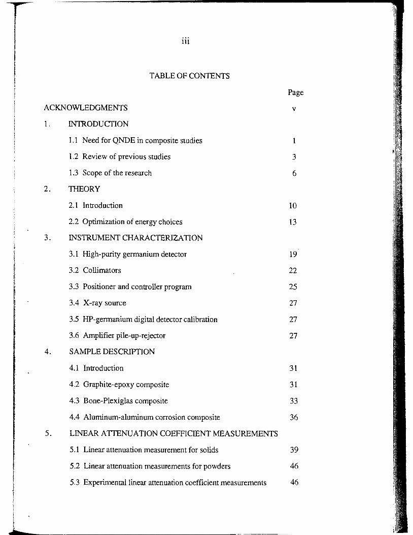
TABLE OF CONTENTS

Page

ACKNOWLEDGMENTS v

I. INTRODUCriON

1.1 Need for QNDE in composite studies I ~ l ;

1.2 Review of previous studies 3 ~' . :··

1.3 Scope of the research 6

2. TIIEORY

2.1 Introduction 10

2.2 Optimization of energy choices 13

3. INSTRUMENT CHARACTERIZATION

3.1 High-purity germanium detector 19

3.2 Collimators 22

3.3 Positioner and controller program 25

3.4 X-ray source 27

3.5 HP-gennanium digital detector calibration 27

3.6 Amplifier pile-up-rejector 27

4. SAMPLE DESCRIPTION

4.1 Introduction 31

4.2 Graphite-epoxy composite 31

4.3 Bone-Plexiglas composite 33

4.4 Aluminum-aluminum corrosion composite 36

5. LINEAR ATTENUATION COEFFICIENT MEASUREMENTS

5.1 Linear attenuation measurement for solids 39

5.2 Linear attenuation measurements for powders 46

5.3 Experimental linear attenuation coefficient measurements 46

lV

5.3.1 Graphite-epoxy composite

5.3.2 Bone-Plexiglas composite

5.3.3 Aluminum-aluminum corrosion composite

6. RESULTS AND DISCUSSIONS

46

53

53

6.l . .Introduction 56

· 6.2 Graphite-epoxy composite measurements 56

6.2.1 Optimization study 56

6.2.2 Graphite-epoxy composite results and discussions 57

6.3 Bone-Plexiglas composite measurements 67

6.3.1 Optimization study 67

6.3.2 Bone-Plexiglas composite results and discussions 70

6.4 Aluminum-aluminum corrosion composite measurements 76

6.4.1 Optimization study

6.4.2 Aluminum-aluminum corrosion composite

results and discussions

7. CONCLUSIONS

REFERENCES

76

76

85

88

v

ACKNOWLEDGMENTS

I would like to thank my major professor Joe Gray for his enthusiasms and

continual support for believing in my research work.

I would also like to acknowledge Terry Jensen for his immaculate care for research

wisdom that has helped propel this work.

I would like to acknowledge all the people who have helped me along the way in

this thesis. To name just a few: Liz Sewik, Vivekend Kini, Sarat Kakumanu, Dave Hsu,

Vinay Dayal, Don Thompson, Mike Hughes, Dick Wallingford, Rick Powell, Thadd

Patton, Libby, Linda, Kim, Susana, Terri, Sara, Connie, lynne.

I would also like to thank my friends Elias, Paul, Bijju, Shabana and Teresa who

have made my studies at Iowa State University more enjoyable.

This work is sponsored by the FAA-Center for Aviation Systems Reliability,

operated by the Ames Laboratory, USDOE, for the Federal Aviation Administration under

Contract No. W-7405-ENG-82 with Iowa State University and NIST under cooperative

agreement #70NANB9H0916.

Government has assigned document number to my thesis IS-T 1640

' ;;

.~

1

1. INlRODUCTION

1.1 Need for ONDE in composite studies

In a wide range of situations the need for characterization of material properties of man­

made and natural materials arises. These situations can include inspection during fabrication of

material, and in-sexvice inspection of mechanical parts as they wear and near their design life.

The need to characterize the material of interest involves all aspects of material performance,

such as: the strength of the material, fracture toughness, density, hardness, material

uniformity, and conductivity, etc. We present here a technique that is capable of quantitatively

determining composition, density and material uniformity. It should be pointed out that no one

technique can measure all properties of interest.

The development of new materials for commercial usage is brought about by increasing

demand for high strength, high fracture toughness, light weight, and low cost of materials.

Very few manufacturing processes can be standardized to guarantee the quality of the product.

If these new materials are to meet the design requirements, some form of testing of the finished

products will certainly be necessary. Therefore, the challenge to the field of nondestructive

evaluation (NDE) is to expand beyond simple flaw detection into material characterization for

the purpose of estimating mechanical and physical properties of the new materials. In this

thesis, a new quantitative NDE x-ray technique is presented that meets this challenge.

Nondestructive material characterization for material variations can be used to achieve higher

reliability in the manufacturing processes, and also can lower life-cycle cost of the product with

in-sexvice NDE inspections. As perfonnance demands for new advanced materials increase, the

manufacturing quality control will become more stringent. Recently, material characterization

for in-sexvice inspection has become an important issue in the commercial aircraft industry. As

2

the world aircraft fleet is becoming older, the material characterization for the purpose of

corrosion detection is extremely important in order to extend the design-life of older aircraft.

The advanced materials that are of interest in this study are composite materials. There

are many types of composites used in structures. The most widely used are low-density

composites consisting of high strength fibers, like glass and carbon, in combination with

thermoset resins such as polyesters and epoxies. This is particularly true for aerospace and

automobile industries. Many conventional alloys in the manufacturing of aircraft and

automobiles and other items are increasingly being replaced by composite materials. The

common composites used are metal-matrix composites and graphite-epoxy composites. This is

mainly because the directional strength and the fracture toughness of the composite products

can be tailored to match the required performances of the mechanical part for load-bearing

purposes; while, at the same time, the composite products can be tailored to minimize the

weight and cost of the material.

Jn NASA Aircraft Energy Efficiency (ACEE) program [14,20,22], which spanned the

mid-70's and into the 80's, applications of advanced composites were demonstrated in

secondary and non-load-bearing primary structures for conunercial transport airplanes. Thus,

as a result, as much as 5% of the structures in newer aircraft such as Boeing 757 and 767 and

the Airbus 320 are being converted from conventional alloys to graphite-fiber-reinforced-epoxy

composites. This is accompanied by weight saving of more than 20% for some airplane

secondary structures such as 727 elevator and DC-10 rudder, and primary structures such as

737 horizontal stabilizer and DC-10 vertical fin [29]. More recently, aircraft such as the Lear

Fan is made almost exclusively of composite materials- about 90% graphite-epoxy composite.

Therefore, over the past decade and a half, extensive research and application development

have produced high performance graphite-epoxy composites with demonstrated material

confidence, and predictability.

3

As aircraft industry advances, the industry pushes the application-envelop of composite

materials. More graphite-composites are beginning to replace metal alloys in primary load­

bearing structures. Thus, there is a demand for more stringent quality control of the composite

and for better understanding of the material characteristics of the product The benefits of

composite materials are sometimes offset as it is difficult to control the manufacturing quality of

the composite products. Composite products, and particularly fiber-reinforced plastics, often

contain defects as a result of normal manufacturing procedures. ln the final composite product,

it is common to find matrix-rich regions and matrix-starved regions and voids. These defects

affect the mechanical properties of the composite products. For example, l% material variation

in graphite-epoxy composite product results in 3% loss of composite strength. It is common to

find material variation of up to 10-15% in graphite-epoxy composite products. Therefore,

quantitative NDE is necessary for manufacturing quality control as well as for in-service

damage detection of composite products.

The application of composites is very broad. Similarly the definition of composite will

be very broad in this thesis work. We define the term composite as any physical system that is

composed of two or more components distinguishable at the macro-level. We will study three

different composite systems in this thesis. They are: graphite-epoxy composite system, bone-

Plexiglas composite system, and a composite system of a metal and its corrosion product. The

emphasis of this thesis is with two-component composite-systems. Nevertheless composite­

systems with more than two components can be handled in the same manner discussed herein.

1.2 Review of previous studies

For traditional nondestructive evaluation by x-ray, conventional radiography using x­

ray films and image intensifiers may be useful in certain cases. These techniques can be used to

identify voids and regions of substantially varying density in simple composites. It is known

4

that a monoenergetic beam can be used for composite material characterization [30], provided it

is a two-component composite, the total thickness of the composite is known and that the

thickness remains constant. An alternative method known as energy-dispersive x-ray is

presented in this thesis to measure material composition avoiding the need to have a constant

total sample thickness. The idea behind the x-ray energy-dispersive technique is based upon the

fact that elements and compounds have characteristic x-ray attenuation as a function of x-ray

energy is shown in Fig. 1.1, and, that the rule-of-mixture holds for x-ray absorption

measurements. This technique permits us to measure material composition in materials having

two or more components. The energies have to be chosen because of the energy dependence of

the elemental linear attenuation coefficients. For photon energy below 100 keY there is an

important contribution to the attenuation coefficient from the photoelectric process, which leads

to a strong dependence of the attenuation coefficient for each element on the atomic number, Z.

At much higher x-ray energy, up to approximately 10 MeV, Compton scattering dominates.

This energy range gives sensitivity, not to atomic number, but to the density of the material [9].

Previous work [16] to measure quantitative resin contents in graphite-epoxy composite

using a x-ray radiography film technique has demonstrated that the technique is inaccurate.

Martin concluded that x-ray films have insufficient sensitivity to detect a small change in

composite density. In addition to this, the x-ray attenuation coefficients of graphite and epoxy­

resin are similar at all energies, so there is not enough contrast in the two material coefficients

to detect the differences on films.

It has been suggested that measurements just made above and below the photoelectric

absorption edge of a selected element would greatly enhance the contrast both in film­

radiography [2,12] and in tomography [23]. Rudich et al. [25] developed a high flux x-ray

tube for high output operation at 6 - 25 ke V range for inspection of light elements such as

graphite-epoxy composite. The inspection takes advantage of higher attenuation variations and

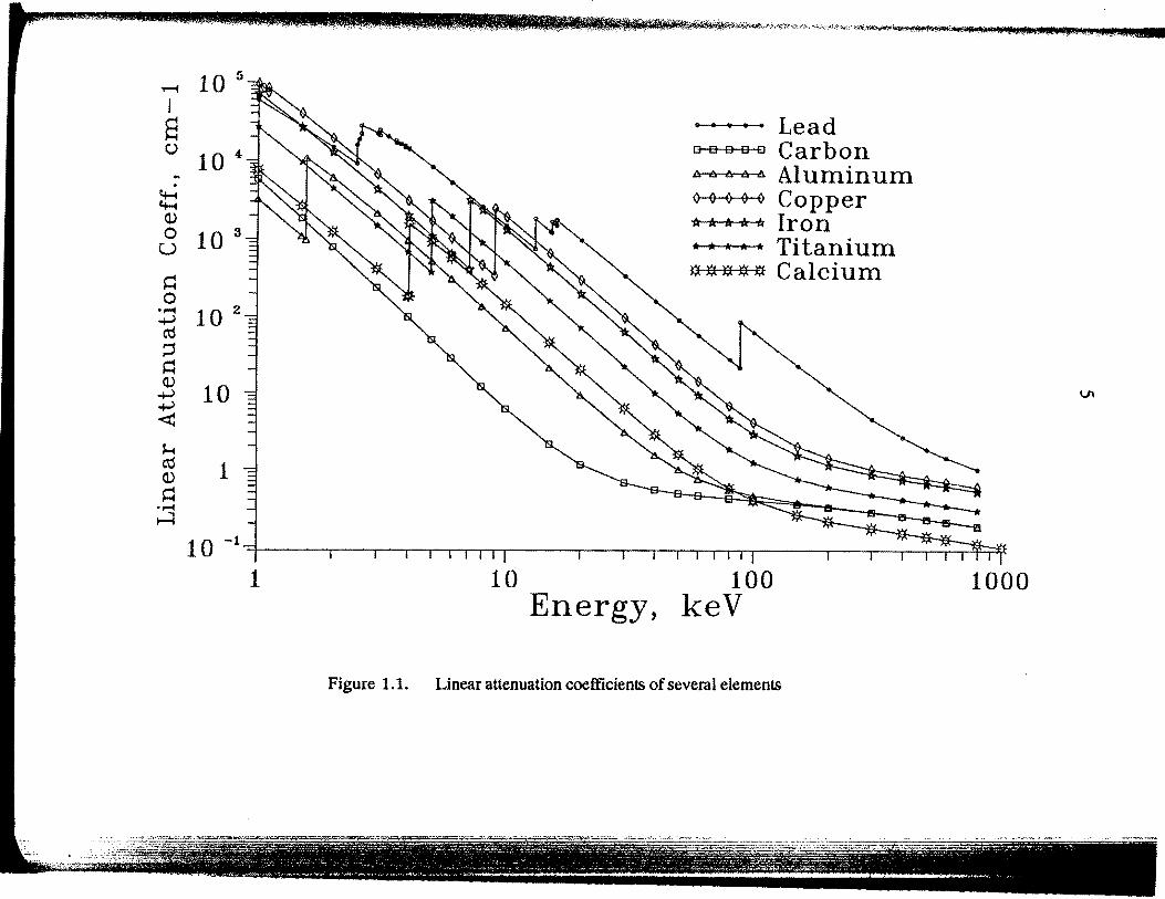
..--4 10 5

I s C)

-. ~ ~ Q.)

10 4

0 10 3 u

~ 0 :;i 10 2

cd ~ ~

2 10 .p..)

< ~ cd (J.)

~ •1""'4 ....:I

1

1

· · · · · Lead o a a a o Carbon 6 6 6 6 a Aluminum o o o o o Copper * * * * * Iron • • • • * Titanium ~ }(( }(( )i( * Calcium

10 100 Energy, keV

Figure 1.1. Linear attenuation coefficients of several elements

1000

6

the photoeletric absorption K-edges, to increase the contrast and resolution to improve flaw

detection. But the locations of the K-edge for carbon, aluminum and calcium are below 5 keV,

thus such a technique is not feasible. In addition, care must be taken when working near the

absorption edge of elements. Kerur et al. have shown that the rule-of-mixture breaks down

when measurements were made at about 471 eV near the K-edge for chromium (8].

The main problem encountered when inspecting light elemental material such as

graphite-epoxy composite is that the x-ray attenuation coefficients of graphite-fibers and epoxy­

resin are similar, as both materials have same basic elemental composition of carbon polymers.

Even then, single energy measurements by Shull et al. have shown promise in quantitative

characterization of porosity in graphite-epoxy composites [26].

The energy-dispersive method has been used in clinical studies for measuring bone

mineral and bone density [5,17, 18,21]. All these studies were made with radioisotope x-ray

sources. This restricted the choice of energies used in this energy-dispersive method. This

problem can be addressed by the use of a x-ray generator and monochromator to select the

desired energies. The use of a monochromator reduces the radiation dosage directly from the x­

ray generator. Our study focus on the choices of x-ray energies by using a x-ray generator, but

we will not address the use of a monochromator. Instead, the energy discrimination and

resolution are resolved with the use of a germanium detector coupled to a multichannel

analyzer.

1.3 Scope of the research

The purpose of this work is to develop a nondestructive evaluation technique by using

x-rays that can quantitatively determine material composition, for material characterization, in

composites. Such information can then be used to estimate the material properties such as the

strength of the composite and the densities of the components.

7

The fact that elements and compounds have characteristic x-ray attenuation that depends

on x-ray energy makes x-ray a natural tool for material characterization. Indeed, the advantages

of this energy-dispersive technique over other x-ray detector systems such as fihns and

fluoroscopy are its increased sensitivity to photon energy and photon intensity. The technique

presented in this thesis work uses a germanium detector coupled to a multichannel analyzer that

allows us to measure the photon intensities and photon counts with respect to energies.

Therefore there is an abundant choice of energies for selection.

X-ray transmission methods can not distinguish the sequencing in which the

components are ordered in a composite product. Thus, in this thesis, the word composite will

not strictly refer to engineered structural composites such as graphite-epoxy composites or

metal-matrix composites. We will restrict ourselves to studying two-component composites,

and we will refer the word composite to any material that has two or more components.

Tirree composite samples studied in this thesis fall into three categories of general

interest; they are: ( 1) a composite system of two materials with similar elemental compositions

and material densities represented by graphite-epoxy composite, (2) a composite system of two

materials with different elemental compositions and material densities represented by bone and

Plexiglas, and (3) a composite system of two materials having approximately the same

elemental compositions with different material densities represented by aluminum 2024 and its

corrosion component. aluminum hydroxide.

The first composite system in this study is a composite of graphite-fibers and epoxy­

resin matrix. Both materials have carbon as their main chemical constituent. Thus their x-ray

linear attenuation coefficients are expected to be similar. The purpose of this study is to

detennine the sensitivity of this technique to measure the material variation in the composite

samples for detennining their fiber-to-resin ratios. Graphite-epoxy composites are increasingly

replacing metal alloys of comparable strength, because graphite-epoxy composite is lighter than

8

metal alloys. Due to manufacturing variability graphite-epoxy composites often contain material

variation in fiber-to-resin ratio. This defect affects the mechanical strength of the composite.

This problem is addressed in this work and x-ray method is developed to measure the non­

unifonnity in composites.

The second composite system is a composite of bone and Plexiglas. We have used

Plexiglas to simulate human tissue. Bone is essentially made of calcium phosphate and

hydroxyappatite, while Plexiglas is made of acrylic; thus the x-ray attenuation coefficients and

material densities are different for the two materials. The bone-Plexiglas composite samples are

used to simulate osteoporosis in a human bone. Osteoporosis is a common bone disease in

adults, where, the bone can lose as much as 40% density [21]. Osteoporosis usually results in

loss of bone material, weakening the bone-strength. Although the osteoporosis usually takes

months or years, early detection of bone loss can in many cases give information to avoid

physical stresses that can result in bone fracture. The purpose of this study is to evaluate the

sensitivity of this energy-dispersive technique in detecting the onset of osteoporosis by

detecting the changes in bone density.

The third composite system is a composite of aluminum 2024 metal alloy and its

corrosion product The x-ray mass attenuation coefficients for the metal and its corrosion

product are essentially the same, but the linear attenuation coefficients are different for the two

components because their densities are different Metal corrosion is of interest in this work,

because metal corrosion is a growing concern in aging aircraft. The purpose of this portion of

the study is to detect small loss in thickness using this x-ray technique. This information will

help detennine the sensitivity attainable using through transmission as a preliminary evaluation

for the on going future development of a back-scatter energy-dispersive technique. The back­

scatter technique can be used as an in-service technique for the detection of metal corrosion in

aging aircraft.

9

The theory of this energy-dispersive technique is presented. The equations described

will be used for the calculations of the results. Since this technique is energy dependent, an

optimization study is conducted to help select the two energies of choice for each of the

composite systems studied. The error estimation is include as part of the optimization study

because it predicts the uncertainties in our experimental measurements. The instrument

verification and experimental procedures are then described. X-ray beam collimation for the

detector and generator will be presented. and their significance will be discussed. This will be

followed by linear attenuation measurement procedures for solids and powers. A novel

technique was developed in this study to measure the linear attenuation coefficients of

powders. Then we will present sample descriptions of the three composite systems we have

mentioned earlier. This is followed by the results and discussions of the experimental

measurements. Experimental material characterization to measure thicknesses and densities of

the components in the composites are presented. Predicted and experimental results are then

compared. Finally, recommendations will be made for future direction of research.

10

2. THEORY

2.1 Introduction

The physics upon which this technique is based depends on the fact that the x-ray

attenuation is a function of both the photon energy and the elemental composition of the

material. When a well-collimated narrow beam of photons passes through a homogeneous

sample of thickness L, the ratio of the transmitted beam intensity I, emerging from the target

along the incident beam direction, to the incident beam intensity 10 is given by Lambert's law,

I _!!. = exp(!lL) I

(1)

This equation assumes that no scattered photons reach the detector, and ll is the linear

attenuation coefficient of the element (ll has unit of cm-1 ). The linear attenuation coefficient is

related to the mean-free-path t by the expression

(2)

The mean free path of a photon, of a given energy traveling in an element, is the

average distance that the photon can travel without interacting with the element. The mass

attenuation is an alternate expression for the attenuation coefficient of an element. The mass

attenuation coefficient ~ ( ~ has unit of cm2/gm), involving the density p, is given by the

expression,

,, I

l

I~

i.ll : J L

t h ! ,, " I i

11

(3)

When the material consists of a chemical compound or of a homogeneous mechanical

mixture such as a composite, the linear attenuation coefficient is given by the weighted sum of

the linear coefficients of the components. This is known as the rule-of-mixture. Thus,

(4)

where ~ is the linear attenuation of the i-th element and wi is its proportion by weight For a

chemical compound with the chemical formula (Zl)a1(Z2)a2 ... (Zn)an, where Zi's are the

atomic number of the elements, the weighting factor for the i-th element, Zi, is given by

(5)

where Aj's are the atomic weight of the element, and aj's are the number of atoms of the

element in the chemical formula [10].

By using Lambert's law and the rule-of-mixtures, we can obtain sufficient information

to determine the constituent materials of the composite by measuring the attenuation of the

initial x-ray beam at a number of selected energies as the beam passes through the composite.

Therefore, the x-ray attenuation in materials can be expressed in the following general form

using Lambert's law and the rule-of-mixtures,

'' !

: J i

12

(6)

where i denotes the components in the composite, and j denotes the energies at which the

parameters are measured. 10 (Ej) is the incident beam intensity, I(Ej) is the transmitted beam

intensity, Xi is the thickness of component i, and J.l.i(Ej) is the linear attenuation coefficient of

component i measured at Ej.

We need a minimum of two energies to study a two component composite. This gives

us the following two equations,

(7a)

(7b)

where

(8)

The linear attenuation coefficients for elements, or compounds, can be either obtained

from experimental measurements or can be obtained from XCOM predictions [3]. Then, by

taking the attenuation measurements of the initial beam at selected energies, we have sufficient

information to solve the two simultaneous equations (7a,7b) and the results are,

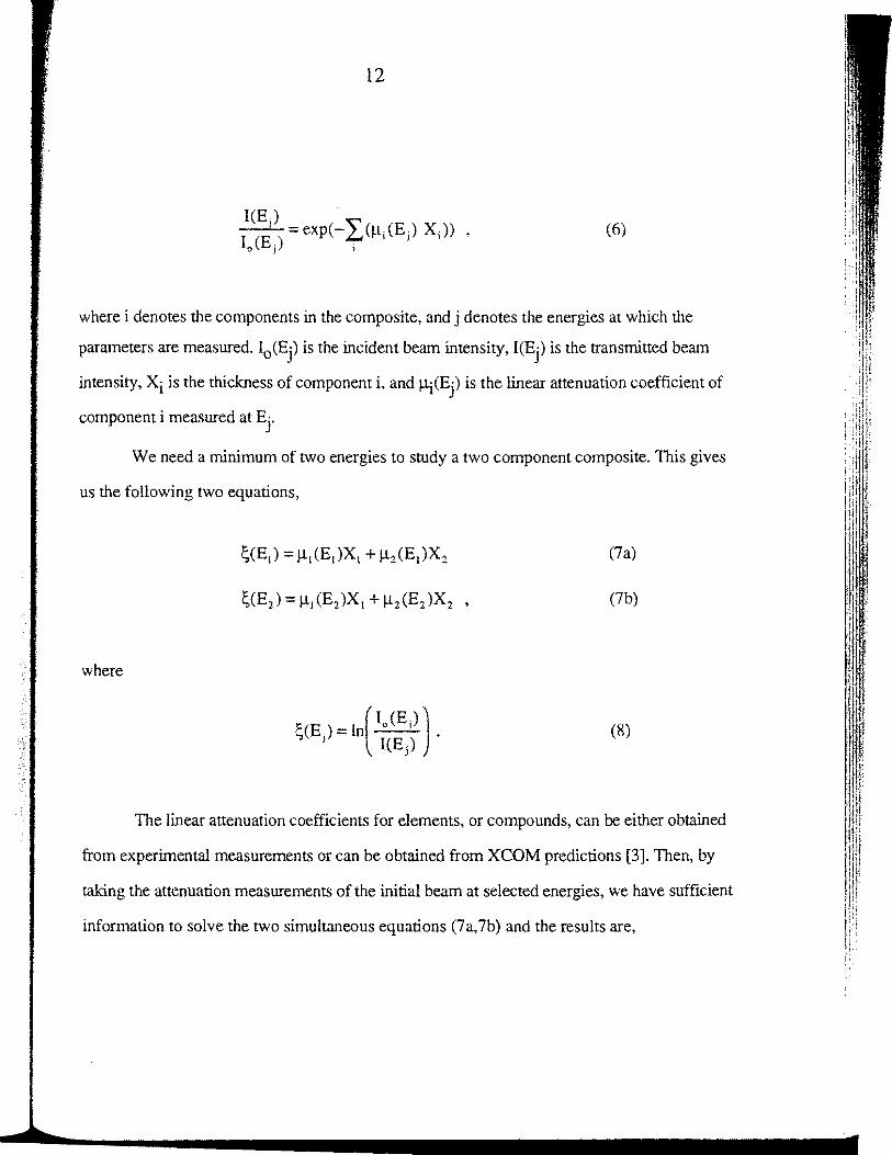
13

XI = ~(El) 112 (E2)- ~(E2) 112 (El)

. llt(Et) 112(E2)-!lt(E2) ll2(E1)

x2

= ~CE2) !11 (Et)- ~(Et) llt (E2)

llt(Et) Jl2(E2)-!lt(E2) !l2(Et)

(9a)

(9b)

Though the work presented here studies two component composites, this does not

exclude the capability of this x-ray technique for studying composites with more than two

components. To study such composites, one needs to measure the attenuation of the beam at

more energies along the x-ray spectrum according to the number of components.

In making these measurements one has the choice of energies to use. There are many

constraints such as x-ray penetration through material, measurement time and maximum energy

of the x-ray source that may influence the energy selections. Thus within these constraints, one

wishes to optimize the accuracy of the thickness detennination. In next section we will derive

the expressions for quantitatively assessing the accuracy of the technique outlined above for a

two component composite.

2.2 Optimization of energy choices

The energy dependence of this technique makes it necessary to define an optimum

energy pair for a two-component composite. An optimum energy pair in Eq.9 will give the

minimum uncertainty for the calculated thicknesses, Xi's. We can derive an expression from

the error-propagation analysis theorem to predict the accuracy of the thickness measurements.

14

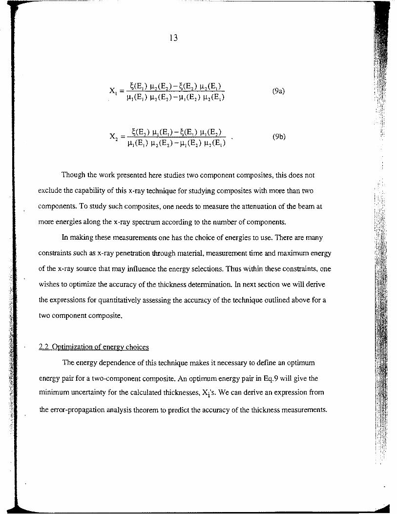
Since this dual energy technique is based on calculating the material thicknesses using

the linear attenuation coefficients of the materials, any source of error in the linear attenuation

coefficients will appear ultimately as error in the thickness determinations. Therefore, we will

first derive an expression to evaluate the uncertainty in the experimentally measured linear

attenuation coefficients. The expression for calculating the linear attenuation coefficients is

given as,

(10)

In general, in error-propagation analysis we do not know the actual errors in any of the

parameters used in the calculations. What we may know instead is some characteristic of the

uncertainty or estimated error of each parameter, such as the standard deviation for each

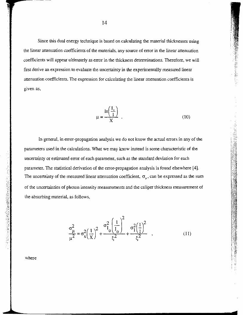
parameter. The statistical derivation of the error-propagation analysis is found elsewhere [4].

The uncertainty of the measured linear attenuation coefficient, cr11

, can be expressed as the sum

of the uncertainties of photon intensity measurements and the caliper thickness measurement of

the absorbing material, as follows,

(ll)

where

,.,_•

·'·

15

(12)

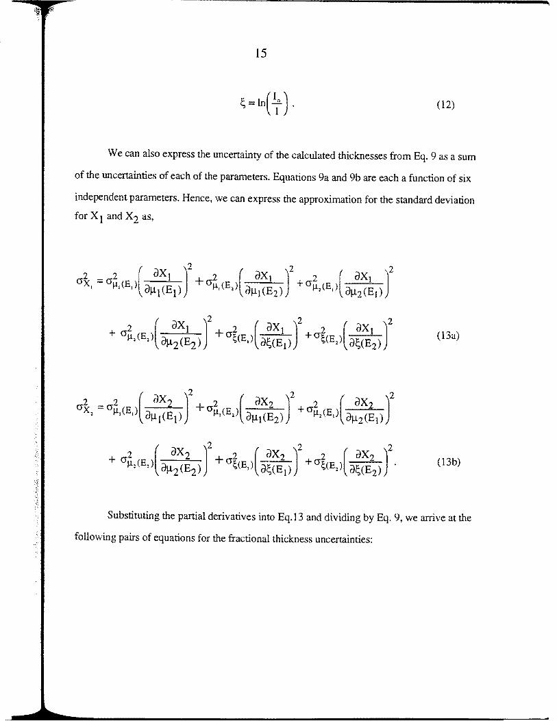
We can also express the uncertainty of the calculated thicknesses from Eq. 9 as a sum

of the uncertainties of each of the parameters. Equations 9a and 9b are each a function of six

independent parameters. Hence, we can express the approximation for the standard deviation

for X 1 and X2 as,

(13a)

(13b)

Substituting the partial derivatives into Eq.13 and dividing by Eq. 9, we arrive at the

following pairs of equations for the fractional thickness uncertainties:

16

and,

(14b)

where

We have shown in our previous study [27] that the uncertainties due to beam

fluctuations can be neglected when more than a million photons are counted. In our experiment

we integrated the incident and transmitted x-ray beam intensities over time to achieve high

counting statistics of over a million counts, and hence we ignored the uncertainties contributed

by the beam intensities in our analysis. The dominating fundamental source of error comes

from the uncertainties in our experimentally measured linear attenuation coefficients. In turn,

17

these linear attenuation coefficient uncenainties are dominated by the caliper thickness

measurements of the absorber. Thus, out of the six original influencing parameters in Eq. 14,

we are left with four significant parameters in our error propagation analysis. These parameters

are the linear attenuation coefficients of the two materials at the two choices of energies.

The optimum energy-pair, predicted by the error-propagation analysis for the minimum

uncertainty, can be found when the two energies are farthest apart fonn one another, even for

cases where the linear attenuation curves intersect one another. The low energy should be

taken, if possible, where the difference in the linear attenuation coefficients is the greatest

between the two materials. This gives maximum contrast for discriminating between the two

materials. The high energy measurement should be made where the difference in the linear

attenuation coefficient between the two materials is the least. Measuring at the high energies

effectively detennines the total thickness of the composite, because the attenuation coefficients

of most materials are similar at these energies. Additional constraints in the choice of energies

are experimental constraints, such as the time required to accumulate high counting statistics

and the ability to accurately measure the attenuation coefficients at the two energies of choice.

Care must be taken in selecting the low energy, E 1, and high energy, Ez. The upper X­

ray energy of the optimum energy pair is naturally constrained by the power output of the X-

ray generator. In addition, measurements made in the upper x-ray energy range are constrained

by the contrast between the transmitted and incident beam intensities, which can be explained

through Eq. 11. At high energies the linear attenuation coefficients are low for all elements,

therefore the difference between the incident and transmitted beam intensities becomes small.

This means the value of ~ is small, and the uncertainty contribution due to 10 and I can be as

large as the uncertainty in the caliper thickness measurement: all this gives rise to large

uncertainties in the linear attenuation coefficient measurements. In contrast. at low energies, the

linear attenuation coefficients are large, consequently, the uncertainties due to the transmission

:i

18

ratio are small. At low energies the uncertainty in the linear attenuation coefficient is sensitive to

the caliper thickness measurement, X. A large absorber thickness will minimize the uncertainty

due to caliper thickness measurements, but it may introduce low transmission beam intensities.

Thus, an absorber thickness should be chosen to closely approach the optimum transmission

ratio, (10 /I), of 3 at the low energies [24].

•i

H il !t

19

3. INSTRUMENT CHARACTERIZATION

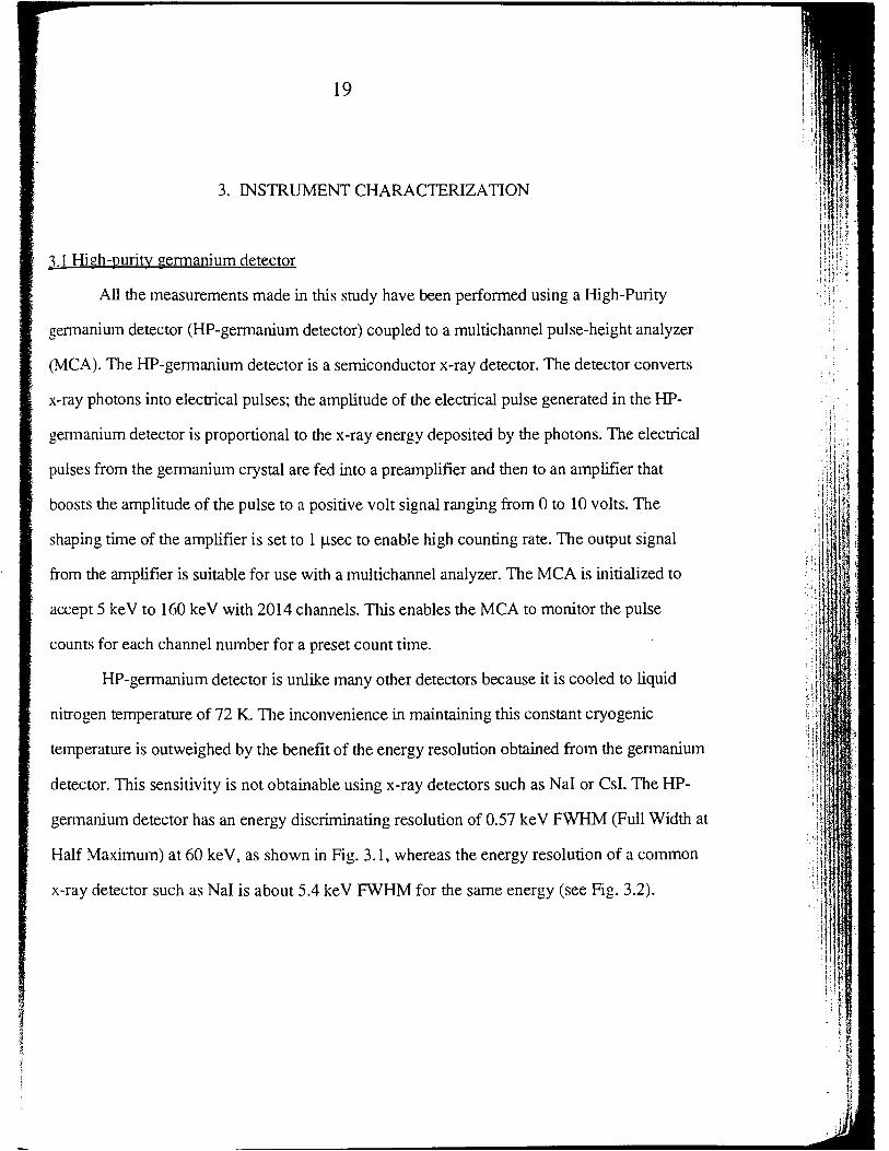
3.1 High-purity germanium detector

All the measurements made in this study have been perlormed using a High-Purity

gennanium detector (HP-gennanium detector) coupled to a multichannel pulse-height analyzer

(MCA). The HP-germanium detector is a semiconductor x-ray detector. The detector converts

x-ray photons into electrical pulses; the amplitude of the electrical pulse generated in the HP­

germanium detector is proportional to the x-ray energy deposited by the photons. The electrical

pulses from the germanium crystal are fed into a preamplifier and then to an amplifier that

boosts the amplitude of the pulse to a positive volt signal ranging from 0 to 10 volts. The

shaping time of the amplifier is set to 1 j.l.Sec to enable high counting rate. The output signal

from the amplifier is suitable for use with a multichannel analyzer. The MCA is initialized to

accept 5 keY to 160 keY with 2014 channels. This enables the MCA to monitor the pulse

counts for each channel number for a preset count time.

HP-germanium detector is unlike many other detectors because it is cooled to liquid

nitrogen temperature of 72 K. The inconvenience in maintaining this constant cryogenic

temperature is outweighed by the benefit of the energy resolution obtained from the germanium

detector. This sensitivity is not obtainable using x-ray detectors such as Nal or Csl. The HP-

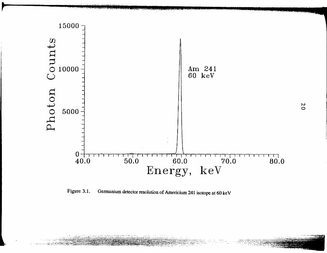
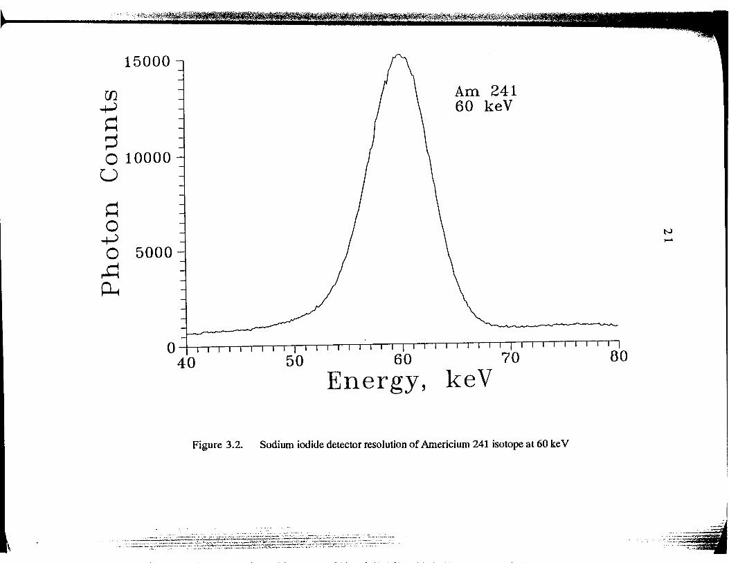
gennanium detector has an energy discriminating resolution of 0.57 keY FWHM (Full Width at

Half Maximum) at 60 keY, as shown in Fig. 3.1, whereas the energy resolution of a common

x-ray detector such as Nal is about 5.4 keY FWHM for the same energy (see Fig. 3.2).

:I

U)

+> ~ ~

15000

0 10000 Am 241 60 keV u

~ 0

+> 0 5000

,..q ~

0~~~~~~~~~~,~~~~~~~~~~TTTIIIIIIII 40.0 50.0 60.0 70.0

Energy, keV

Figure 3.1. Germanium detector resolution of Americium 241 isotope at 60 keV

lfJ. ..,_~

~ ~

15000

0 10000 u

~ 0

..,_~

0 5000 ~ ~

Am 241 60 keV

Q~~~~~~~~~~~~IITTIIIIIIITTTIIIIIIn

40 50 60 70 Energy, keV

Figure 3.2. Sodium iodide detector resolution of Americium 241 isotope at 60 keV

-·-·" -- -- -----·- ". ~·· -···· ·' ,.~- . -- •. : -~ ;::::::=~:~;;;<:~~:;;;;:~:=~¥~~r~~~~=:=~:2~~E3~~?~H;<~c?:~~i~;:(:":~=":=:::=. ~~

I --.···~·-·-._ ... ·. :_. ;.;;.:;::--:-- . '~. '

-<o 0 ~~c•

22

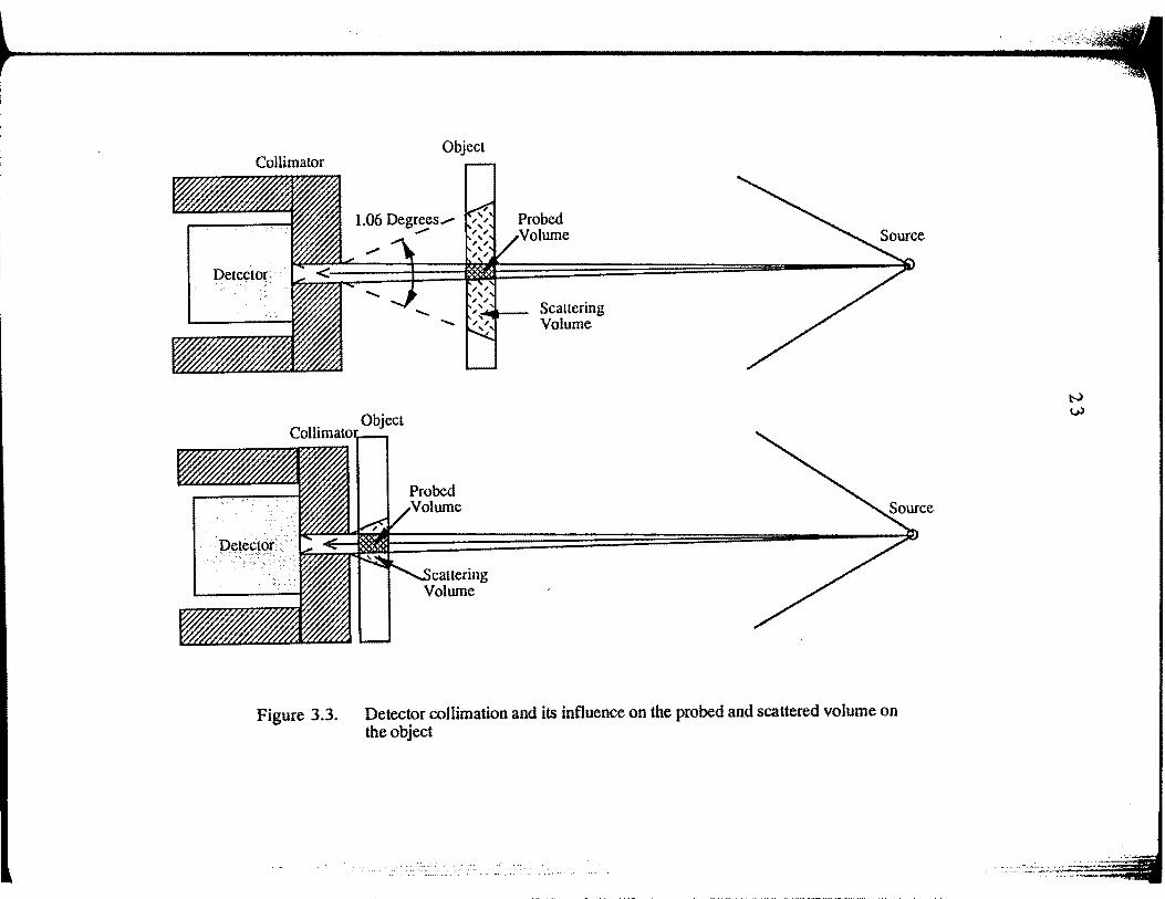
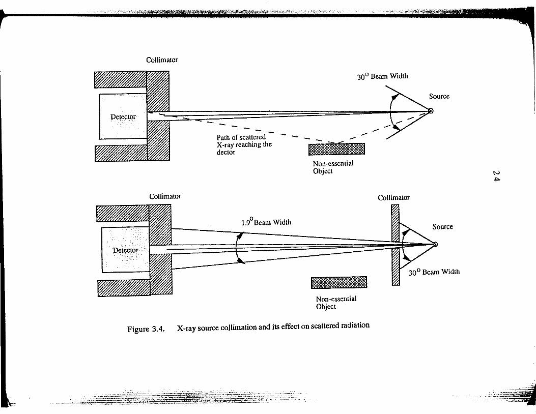
3.2 Collimators

Collimators in the experimental setup are used to define the narrow pencil beam

configuration that is necessarily assumed from Lambert's law. The collimation setup also

suppresses the background due to scattered x-rays from non-essential objects in the x-ray

vault. Thus the collimation defmes the volume of the object probed by the x-ray beam.

The HP-germanium detector is shielded in a quarter inch thick lead box as shown in

Fig. 3.3. A collimator hole of 350 micron diameter defines the diameter of the probed volume

on the sample. This also reduces the intensity of incident, and scattered, photons reaching the

detector. The detector collimation reduces the intake of scattered photons to be within a cone-

arc of 1.06 degrees, approximately.

It is important to shield the non-essential objects, that would typically be illuminated by

the x-ray generator, scattering incident x-rays that may reach the detector. Non-essential object~

lying between the source and the detector are shielded from the beam by the source-collimation

as indicated in Fig 3.4. The source-collimator essentially eliminates x-ray scattering from non-

essential objects that would typically be illuminated by the x-ray source by reducing the cone­

beam from 30 degrees to 1.9 degrees. It is also important to note the presence of the detector­

collimator and the positioning of the object between the source and the detector; because, in

some cases the coherent and incoherent scattering may reach the detector, giving too high a

value for the transmitted intensity. The detector-collimator determines the volume of the object

probed. Even so, the detector also picks up signals of scattered x-rays from the scattering-

volume in the object. One can reduce much of this scattering volume by positioning the object

closer to the detector. A smaller collimation hole can equally reduce the scattering volume on

the object, but this would also proportionally reduce the incident X-ray beam intensity. If a

radioactive isotope source were used it would be necessary to balance the collimator size for the

detector while maintaining sufficiently high incident x-ray beam intensity for statistical

' ~ .

Object

Probed Volume

Scattering Volume

Figure 3.3. Detector collimation and its influence on the probed and scattered volume on the object

Collimator

Collimator

-Path of scattered X-ray reaching the dec tor

1.9° Beam Width

-Non-essential Object

Non-essential Object

30 ° Beam Width

Source

--

Collimator

30° Beam Width

Figure 3.4. X-ray source collimation and its effect on scattered radiation

25

purposes. By using an x-ray generator as the source, we can overcome this statistical limitation

by increasing the current generating the x-ray beam.

3.3 Positioner and controller program

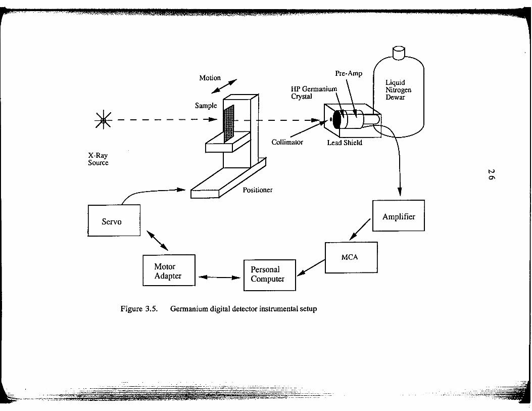
The block diagram of the experimental setup of the electronic communication between

the PC and the detector and positioner is shown in Fig. 3.5. The positioners (Daedallnc.) are

used to move the sample object during an experiment by precision stepper motors

(Compumotor Inc.). The motors are controlled with a DELL 386 PC using a Compumotor PC-

23 indexer board placed in the computer. The indexer board sends commands to, and receives

positioner status from, the motor adapter. The adapter in turns sends commands to the motor,

through a motor servo, instructing how much the motor should rotate for a given travel

distance. The stepper motor has stepping resolution of l 00,000 steps per inch. This gives us a

precision if 10 1.1. inch to move the sample back and forth on the positioner.

A typical experimental measurement in this study takes up to 24 hours to acquire

sufficient statistics of over a million counts for the beam intensities, I and 10 . By moving the

object in and out of the x-ray beam, the program can monitor the x-ray beam instability over

time. The two beam intensities are integrated over time to obtain the transmission ratios.

Therefore a controller program was developed to automatically move the sample on the

positioner in and out of the x-ray beam at preset time intervals to collect the transmitted and the

incident beam intensities, respectively. The controller program was developed to allow the

operator to interactively create an energy bin array with tailored energy bin sizes. The

positioner movement and data acquisition from the MCA are controlled using the PC with a

C++ driver program called "MCA_2."

;.

•.·

Sample

*-------~ X-Ray Source

Servo

---

Motor Adapter ... Personal

Computer

Figure 3.5. Germanium digital detector instrumental setup

Pre-Amp Liquid Nitrogen Dewar

Amplifier

/ L.----.---1

MCA

27

.1,_4 X-Ray source

The x-ray source used in this work is a Ridge HOMX 160A microfocus generator with

a 10 micron focal spot size approximately. The generator provides a Bremsstrahlung spectrum

to measure the attenuation coefficients. The energies of the spectrum are resolved using the

MCA. The generator is capable of operating at energies up to 160 ke V and with beam currents

of up to 2 mA. It should be mentioned that this energy sensitive technique was also

successfully demonstrated with the use of radioisotope sources [27]. Therefore the microfocus

capability is not a required feature for the x-ray generator; indeed, any radiation sources could

have been used for this study.

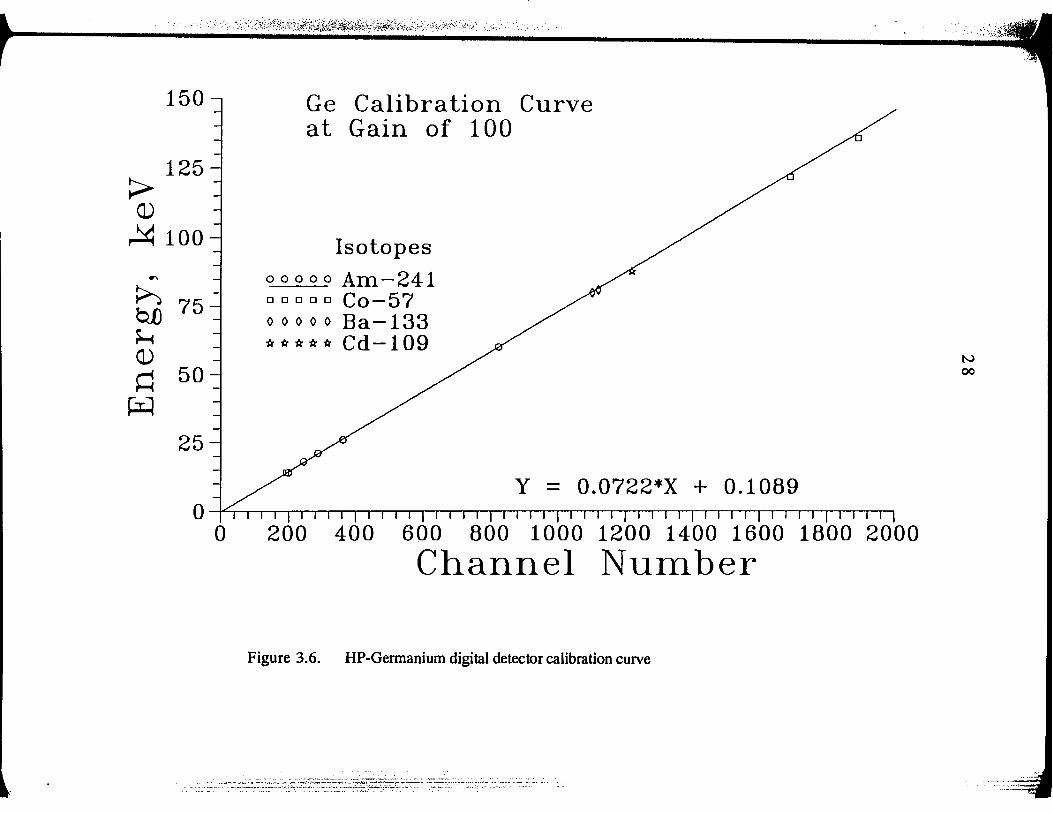
3.5 HP-Germanium digital detector calibration

Calibration of the HP-gerrnanium digital detector with the MCA setup is necessary to

correlate the MCA channels to the x-ray energies. We used radioactive isotopes to calibrate the

detector system. Radioactive isotopes emit well-defined x-ray energies and these energies show

up as sharp peaks on the MCA spectrum. Thus, a linear detector calibration curve can be

developed with sufficient number of radioactive isotopes as plotted in Fig 3.6. The present

energy sensitivity of the MCA in this study is 12 channels per keV.

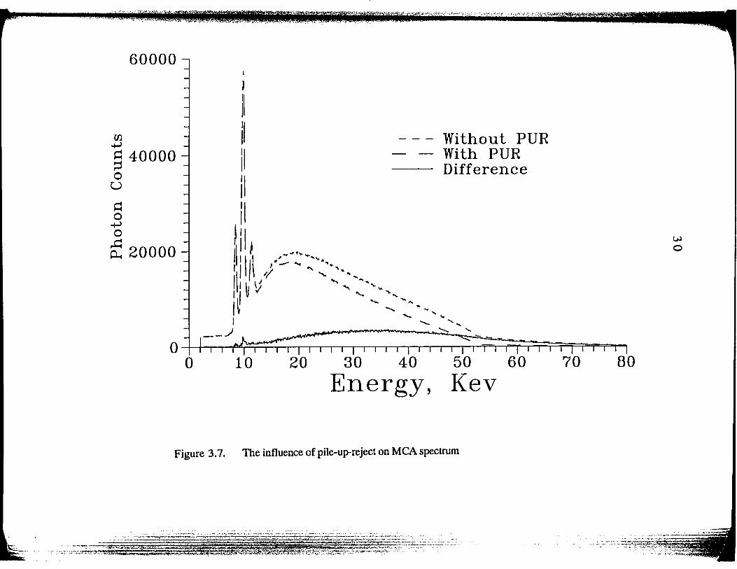
3.6 Amplifier pile-up reiecter

X -ray spectral distortion is often found during high counting rates. This spectral

distortion caused by signal pile-up usually occurs when two or more x-ray photons strike the

detector at close time intervals. In such instances, the germanium detector electronics is unable

to resolve each signal generated by the photons. Thus the electrical signals are summed into

one larger signal. This count rate limitation is strictly related to the number of input counts per

unit of time and is independent of energy [1]. Consequently, the spectral distortion in the

150

125 >

Cl)

~ 100

25

Ge Calibration Curve at Gain of 100

Isotopes o o o o o Am- 2 41 o o o o o Co-57 ooooo Ba-133 ***** Cd-109

Y = 0.0722*X + 0.1089 o~~~~~~~~~~~~~~~~~~~~~~~~~~

0 200 400 600 800 1000 1200 1400 1600 1800 2000

Channel Number

Figure 3.6. HP-Germanium digital detector calibration curve

N 00

29

Bremsstrahlung spectrum will show more photon counts at higher energies than in reality. This

is a problem because this x-ray energy-dispersive technique is energy sensitive. The Canberra

amplifier used here has an efficient pile-up rejecter (PUR). The PUR provides an output logic

pulse for the associated multichannel analyzer to suppress the spectral distortion caused by high

counting rates. The effect of the PUR on the spectrum can be seen in Fig 3.7.

-. ~ ' .. ; . '

rn ~

• " f,:i.: ... ~ • '-'-~~ .,,-~-:;..._ ~·-" ,.[ .;~ ·,. .... :si:l. ~,....:;t( "' ',:r,;:. w.:

.,_• ' 1

.f<O/ i!cl L "• '-> I ~ ' ' ''"o~1 ' • ' I

60000

§ 40000 0 u ~ 0 ~ 0 s: 20000

Without PUR With PUR Difference

o4+~~~~~~~~~~~~~~~~~~ 0 10 20 30 40

Energy, 50 60

Kev

Figure 3.7. The influence of pile-up-reject on MCA spectrum

70 80

31

4. SAMPLE DESCRIPTION

4.1 Introduction

Three different composite systems were investigated in this study. The first composite

system is a graphite-epoxy composite, consisting of two materials, graphite-fibers and epoxy­

resin, having very similar elemental compositions and densities. The second composite system

is a bone-tissue composite, consisting of two materials having very different elemental

compositions and densities. The third is a composite system of aluminum 2024 metal and its

corrosion product composed of two materials with similar elemental composition, but very

different densities. The following subsections describe the materials used in the composites and

the quantitative composition of each of the components used in the composite samples.

4.2 Graphite-epoxy composite

Graphite-fiber-reinforced-epoxy composite (graphite-epoxy composite) is increasingly

replacing metal alloys because the selective directional strength of the composite can be tailored

to match the required strength performances for load bearing; while, at the same time, the

composite material is lighter than metal alloys having comparable strength.

The graphite-epoxy composite used in this study is made from Magnarnite 8551-7

uniaxial prepreg sheets manufactured by Hercules Inc. This composite is considered to be the

next-generation composite because this amine-cured epoxy-resin is doped with micro-spheres.

This makes the composite more impact resilient The graphite fiber in Magnamite 8551-7 is a

synthetic polyacrylonitrile (PAN-based) graphite fiber known as IM-7 fiber. Samples of neat-

epoxy-resin were provided by Hercules Inc. for linear attenuation coefficient measurements.

We were also able to obtain some graphite fibers, but the graphite fibers have diameter of 5

' ''·

:I ll.

':lr

32

~m, and this made the linear attenuation coefficient measurement difficult. The determination of

the linear attenuation coefficients for the materials is deferred to Section 5.

A sample of Magnamite composite was fabricated at Iowa State University's

Aerospace Engineering and Engineering Mechanics departmental composite laboratory. The

lay-up and curing procedure for the Magnamite composite follows that described in the

International Encyclopedia of Composites [13]. The composite lay-up is 0/90 with a total of 23

layers. The final thickness of the composite is 0.457 em after curing.

A coupon from the Magnamite composite, size 2.5 em by 2.5 em, by 0.457 em thick,

is analyzed to determine the effective total thickness of the IM-7 fibers and epoxy-resin in the

23 layers. This was needed for comparison with the x-ray measured thickness values. A corner

of the composite coupon was chosen for analysis. The assumptions are that the fiber-to-resin

ratio variation at the localized corner of the coupon is small, and that the fibers are

perpendicular to the side-faces of the corner.

The two adjacent surfaces to the corner were polished to produce surfaces that exposed

the ends of the fibers. We took black-and-white photomicrographs at layers that have exposed

fiber-ends. The photomicrographs are taken at a magnification of 300. Two arrays, of 6

columns by 12 rows, and 6 columns by 13 rows, of photomicrographs are taken of the two

polished surfaces on either side of the selected corner. The two arrays covered an area of 0.310

em by 0.457 em, approximately, on either side of the corner.

An image processing technique is used to detennine the fiber-to-resin ratio in each

photomicrograph. The black-and-white photographs are digitized using a camera-digitizer; the

image is acquired through a PC based image acquisition software. The digitized data are

transferred to an image analysis software based on a Macintosh computer. A black-and-white

thresholding technique is used to determine the fiber-to-resin ratio in each photomicrograph.

The fiber-to-resin ratios ofthe micrographs are averaged in 12 columns in the thickness

1.

. ' i

33

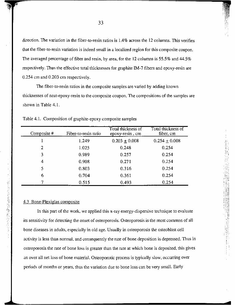
direction. The variation in the fiber-to-resin ratios is 1.4% across the 12 columns. This verifies

that the fiber-to-resin variation is indeed small in a localized region for this composite coupon.

The averaged percentage of fiber and resin, by area, for the 12 columns is 55.5% and 44.5%

respectively. Thus the effective total thicknesses for graphite IM-7 fibers and epoxy-resin are

0.254 em and 0.203 em respectively.

The fiber-to-resin ratios in the composite samples are varied by adding known

thicknesses of neat-epoxy-resin to the composite coupon. The compositions of the samples are

shown in Table 4.1.

Table 4.1. Composition of graphite-epoxy composite samples

Total thickness of Total thickness of Composite# Fiber-to-resin ratio epoxy-resin , em fiber, em

1.249 0.203 ± 0.008 0.254 ± 0.008

2 1.025 0.248 0.254

3 0.989 0.257 0.254

4 0.908 0.271 0.254

5 0.803 0.316 0.254

6 0.704 0.361 0.254

7 0.515 0.493 0.254

4.3 Bone-Plexiglas composite

In this part of the work, we applied this x-ray energy-dispersive technique to evaluate

its sensitivity for detecting the onset of osteoporosis. Osteoporosis is the most common of all

bone diseases in adults, especially in old age. Usually in osteoporosis the osteoblast cell

activity is less than normal, and consequently the rate of bone deposition is depressed. Thus in

osteoporosis the rate of bone loss is greater than the rate at which bone is deposited, this gives

an over all net loss of bone material. Osteoporotic process is typically slow, occurring over

periods of months or years, thus the variation due to bone loss can be very small. Early

i i

34

detection of bone loss can give information ro avoid physical stress that can result in bone

fractures.

If we classify the body parts of a human in terms of their respective densities. we can,

in general, view the human body as a two component composite consisting of bone and soft-

tissues (flesh). ln this study we wish to determine the thicknesses of flesh and density of bone

in our samples using this x-ray energy-dispersive technique for detecting the onset of

osteoporosis.

We made our own samples to simulate body parts of a human subject We used dense

bone samples from a cow to simulate human bone in our study. A cattle femur bone was cut to

produce parallel surfaces where the thicknesses are known. The density of the cattle bone

sample is 2.077 gm/cm3. This is determined from mass and volume measurements of the bone

sample. Plexiglas is used to simulate soft-tissue in this study. Plexiglas is chosen because it

will not decompose like meat at room temperature during our long data acquisition time. In

addition, Plexiglas is commonly used as a standard calibration material, for the same reason

mentioned above, in medical X-ray CAT scan to simulate soft-tissue.

Two sets of samples are made to simulate two different parts of a human patient. One

set of samples has the bone and Plexiglas thicknesses of 0.808 em and 0.925 em respectively.

This set of samples simulates the fingers of the patient Another set of samples simulates the

calf of the patient The thicknesses of the second set of samples of bone and Plexiglas are

2.400 em and 1.834 em respectively. Two sets of samples were investigated to determine the

accuracy of this x-ray technique to detect the onset of osteoporosis on different body parts with

different thicknesses. During osteoporosis, the outer diameter of the bone does not change;

only the density of the bone changes. Similarly, then. we can have the outer dimensions of the

bone (0.808 em and 2.400 em) in the two sets of bone samples remain the same. Then, by

.':}

35

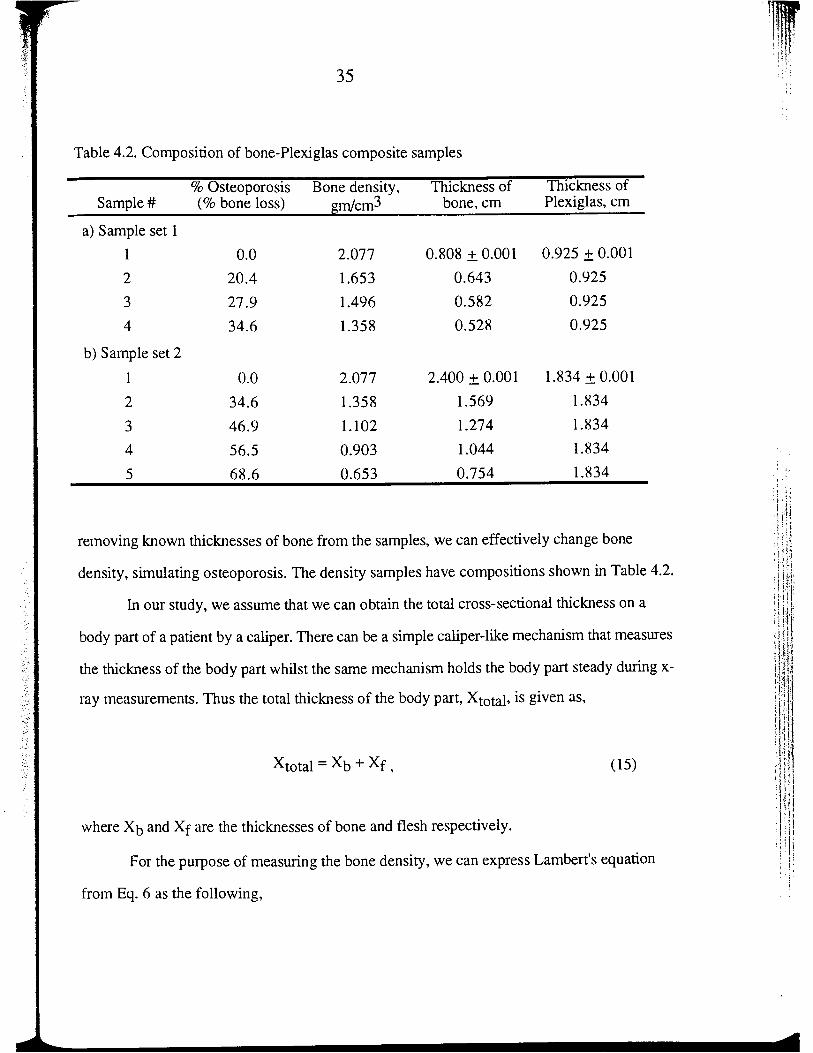
Table 4.2. Composition of bone-Plexiglas composite samples

% Osteoporosis Bone density, Thickness of Thickness of Sample# (% bone loss) gm/cm3 bone, em Plexiglas, em

a) Sample set 1

1 0.0 2.077 0.808 ± 0.001 0.925 ± 0.001

2 20.4 1.653 0.643 0.925

3 27.9 1.496 0.582 0.925

4 34.6 1.358 0.528 0.925

b) Sample set 2

1 0.0 2.077 2.400 ± 0.001 1.834 ± 0.001

2 34.6 1.358 1.569 1.834

3 46.9 1.102 1.274 1.834

4 56.5 0.903 1.044 1.834

5 68.6 0.653 0.754 1.834

removing known thicknesses of bone from the samples, we can effectively change bone

density, simulating osteoporosis. The density samples have compositions shown in Table 4.2.

In our study, we assume that we can obtain the total cross-sectional thickness on a

body part of a patient by a caliper. There can be a simple caliper-like mechanism that measures

the thickness of the body part whilst the same mechanism holds the body part steady during x­

ray measurements. Thus the total thickness of the body part, X total• is given as,

(15)

where Xb and Xf are the thicknesses of bone and flesh respectively.

For the purpose of measuring the bone density, we can express Lambert's equation

from Eq. 6 as the following,

36

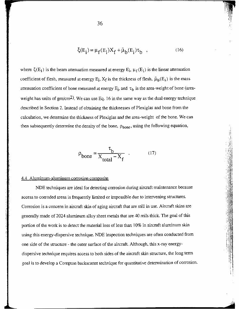
(16)

where ~(Ei) is the beam attenuation measured at energy Ei. llf (Ei) is the linear attenuation

coefficient of flesh, measured at energy Ei, Xf is the thickness of flesh, jlb(Ei) is the mass

attenuation coefficient of bone measured at energy Ei, and tb is the area-weight of bone (area-

weight has units of gm/cm2). We can use Eq. 16 in the same way as the dual energy technique

described in Section 2. Instead of obtaining the thicknesses of Plexiglas and bone from the

calculation, we detennine the thickness of Plexiglas and the area-weight of the bone. We can

then subsequently determine the density of the bone, Pbone• using the following equation,

't p = b

bone X 1- Xf tota

(17)

4.4 Aluminwn-aluminum corrosion composite

NDE techniques are ideal for detecting corrosion during aircraft maintenance because

access to corroded areas is frequently limited or impossible due to intervening structures.

Corrosion is a concern in aircraft skin of aging aircraft that are still in use. Aircraft skins are

generally made of 2024 aluminum alloy sheet metals that are 40 mils thick. The goal of this

portion of the work is to detect the material loss of less than 10% in aircraft aluminum skin

using this energy-dispersive technique. NDE inspection techniques are often conducted from

one side of the structure- the outer surface of the aircraft. Although, this x-ray energy-

dispersive technique requires access to both sides of the aircraft skin structure, the long tenn

goal is to develop a Compton backscatter technique for quantitative determination of corrosion.

'· .,

37

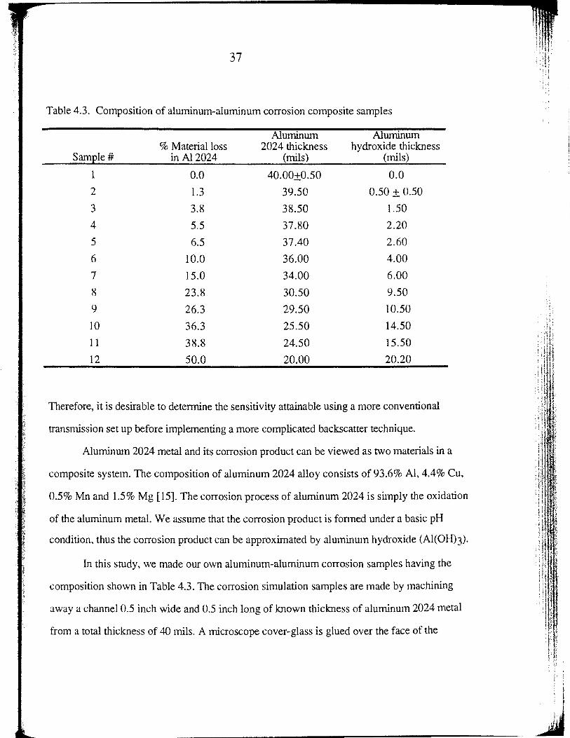
Table 4.3. Composition of aluminum-aluminum corrosion composite samples

Aluminum Aluminum % Material loss 2024 thickness hydroxide thickness

SamEle# in Al2024 (mils) (mils)

1 0.0 40.00±0.50 0.0

2 1.3 39.50 0.50 ± 0.50

3 3.8 38.50 1.50

4 5.5 37.80 2.20

5 6.5 37.40 2.60

6 10.0 36.00 4.00

7 15.0 34.00 6.00

8 23.8 30.50 9.50

9 26.3 29.50 10.50

10 36.3 25.50 14.50

II 38.8 24.50 15.50

12 50.0 20.00 20.20

Therefore, it is desirable to determine the sensitivity attainable using a more conventional

transmission set up before implementing a more complicated backscatter technique.

Aluminum 2024 metal and its corrosion product can be viewed as two materials in a

composite system. The composition of aluminum 2024 alloy consists of 93.6% AI, 4.4% Cu,

0.5% Mn and 1.5% Mg [15]. The corrosion process of aluminum 2024 is simply the oxidation

of the aluminum metal. We assume that the corrosion product is formed under a basic pH

condition, thus the corrosion product can be approximated by aluminum hydroxide (Al(OH)3).

In this study, we made our own aluminum-aluminum corrosion samples having the

composition shown in Table 4.3. The corrosion simulation samples are made by machining

away a channel 0.5 inch wide and 0.5 inch long of known thickness of aluminum 2024 metal

from a total thickness of 40 mils. A microscope cover-glass is glued over the face of the

"!

'

I _j

38

channel. Then, the space beneath the cover-glass is ultrasonically packed with aluminum

hydroxide powder. The thickness of the cover-glass is approximately 8 mils. During beam

attenuation measurements on the corrosion samples, another cover-glass with identical

thickness is used to attenuate the incident beam. This is done to compensate the attenuation

effect of the cover-glass in the beam attenuation measurements.

39

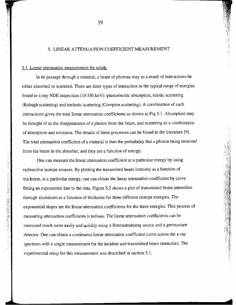
5. LINEAR A ITENUA TION COEFFICIENT MEASUREMENT

5.1 Linear attenuation measurement for solids

In its passage through a material, a beam of photons may as a result of interactions be

either absorbed or scattered. There are three types of interaction in the typical range of energies

found in x-ray NDE inspection (10-350 keY): photoelectric absorption, elastic scattering

(Raleigh scattering) and inelastic scattering (Compton scattering). A combination of such

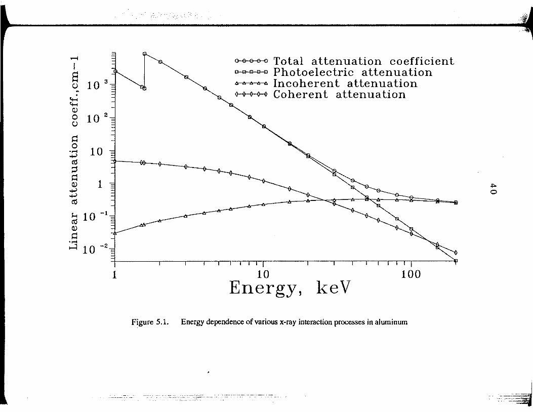
interactions gives the total linear attenuation coefficients as shown in Fig.5.1. Absorption may

be thought of as the disappearance of a photon from the beam, and scattering as a combination

of absorption and emission. The details of these processes can be found in the literature [Y].

The total attenuation coefficient of a material is then the probability that a photon being removed

from the beam in the absorber, and they are a function of energy.

One can measure the linear attenuation coefficient at a particular energy by using

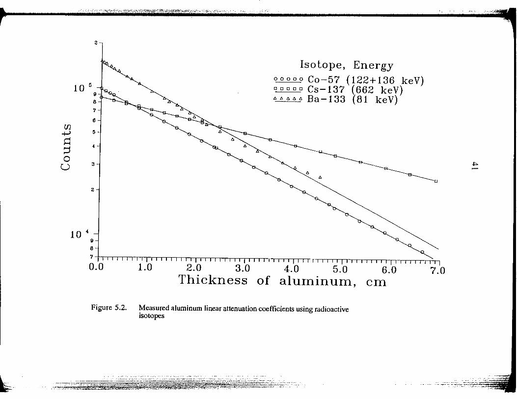
radioactive isotope sources. By plotting the transmitted beam intensity as a function of

thickness, at a particular energy, one can obtain the linear attenuation coefficient by curve

fitting an exponential line to the data. Figure 5.2 shows a plot of transmitted beam intensities

through aluminum as a function of thickness for three different isotope energies. The

exponential slopes are the linear attenuation coefficients for the three energies. This process of

measuring attenuation coefficients is tedious. The linear attenuation coefficients can be

measured much more easily and quickly using a Bremsstrahlung source and a germanium

detector. One can obtain a continuous linear attenuation coefficient curve across the x-ray

spectrum with a single measurement for the incident and transmitted beam intensities. The

experimental setup for this measurement was described in section 3.1.

~~ : tj I : I ~ : :;

. '. t (\

:'if

\rf ' ~

~ i ,, l

~

I

§ 10 3 ~ . ~ ~ Q)

0 10 2 C)

1

Figure 5.1.

-- .. ~·~·~ ... - .. - .. ---··· .

o o o o o Total attenuation coefficient o 8 8 8 c Photoelectric attenuation 6 6 6 6 .e. Incoherent attenuation o 11 11 o ~ Coherent attenuation

10 100 Energy, keV

Energy dependence of various x-ray interaction processes in aluminum

·, ··. \,:

10 5

Isotope, Energy ooooo Co-57 (122+136 keV) ooooo Cs-137 (662 keV) 6 6 6 6 6 Ba-133 {81 keV)

10 4

3

0.0 1.0 2.0 3.0 4.0 5.0 Thickness of aluminum,

Figure 5.2. Measured aluminum linear attenuation coefficients using radioactive isotopes

--·--· --·--· . . ··~ ... ·-- . ·-·· ... .. . -- . -

__ ,"7:::~~;-::~~,~~:1.2::::2~~f~x~••?#tftE~~:~:_~;c_;::;;.s:~:::::·:=:~-; __ _

6.0 em

7.0

42

We have relied on the values for linear attenuation coefficient measured by us because

there are differences in the values of attenuation coefficients in the literature [ 11 ]. Typical

referenced attenuation values have uncertainties of 5% to 10% [ 19]. Deslattes has suggested

that one should not rely on international tables for attenuation coefficients to better than 10%

[6]. In addition, it is important that the transmission attenuation measurements be made with

the same experimental setup as for the beam attenuation coefficient measurements. This is

because differences in beam attenuation due to beam geometry can greatly effect the energy-

dispersive measurements. In particular, one should not use "broad" beam attenuation

coefficients for calculation with "narrow" beam transmission measurements, and vice versa.

In accordance with Lambert's law, the experimental setup requires narrow "pencil­

beam" geometry, i.e., both the source and detector being well collimated. The positioning of

the absorber immediately in front of the detector was chosen because it effectively minimized

the scattered radiation, from the absorber, from reaching the detector. Thus the accuracy of the

linear attenuation coefficient and beam attenuation measurements, for the absorber will be

dependent on how much of the small angle scattering is registered as part of the transmitted

beam intensities.

The collimated x-ray beam is recorded with the HP-germanium detector connected to a

multichannel pulse-height analyzer. The absorber was placed between the x-ray source and the

detector, with the absorber surface perpendicular to the x-ray beam. If a thick absorber is

placed in the beam, the transmitted beam intensity will be low and a relatively long time will be

required to accumulate sufficient counts. In fact, for undesirable low transmissions, the

magnitude of the transmitted beam may be comparable to the background. On the other hand, if

a very thin absorber in used, the transmitted beam intensity approaches that of the incident

beam intensity, and the transmission ratio becomes unfavorable. In our experiment some

intermediate transmission ratio was employed. The absorber thickness was chosen to give a

: ::

43

transmission (lofl) value of 1.1 to 5, thus closely approaching the optimum attenuation

condition with transmission ratio of 3 [24].

The value of the linear attenuation coefficient was calculated using the caliper measured

thickness of the absorber, according to Eq. 10. A correction for air displaced by the absorber

thickness is negligible for solid absorber, because the magnitude of the air attenuation is

negligible compared to the solid. Rather, the main uncertainty in our linear attenuation

measurements is from measuring the thickness of the absorber specimens using a caliper. From

equation 12 we find that the uncertainty in the absorber thickness is the dominating term for

low energy X-rays, because the transmission ratio is high at these energies. On the other hand,

the contribution due to the absorber thickness and beam intensity measurements can be nearly

equal for high energy X-rays when the transmission ratio is small at these energies [7].

A series of measurements with the absorber in and out of the beam was taken to obtain

the transmitted beam and incident beam intensities respectively. Each set of intensities was

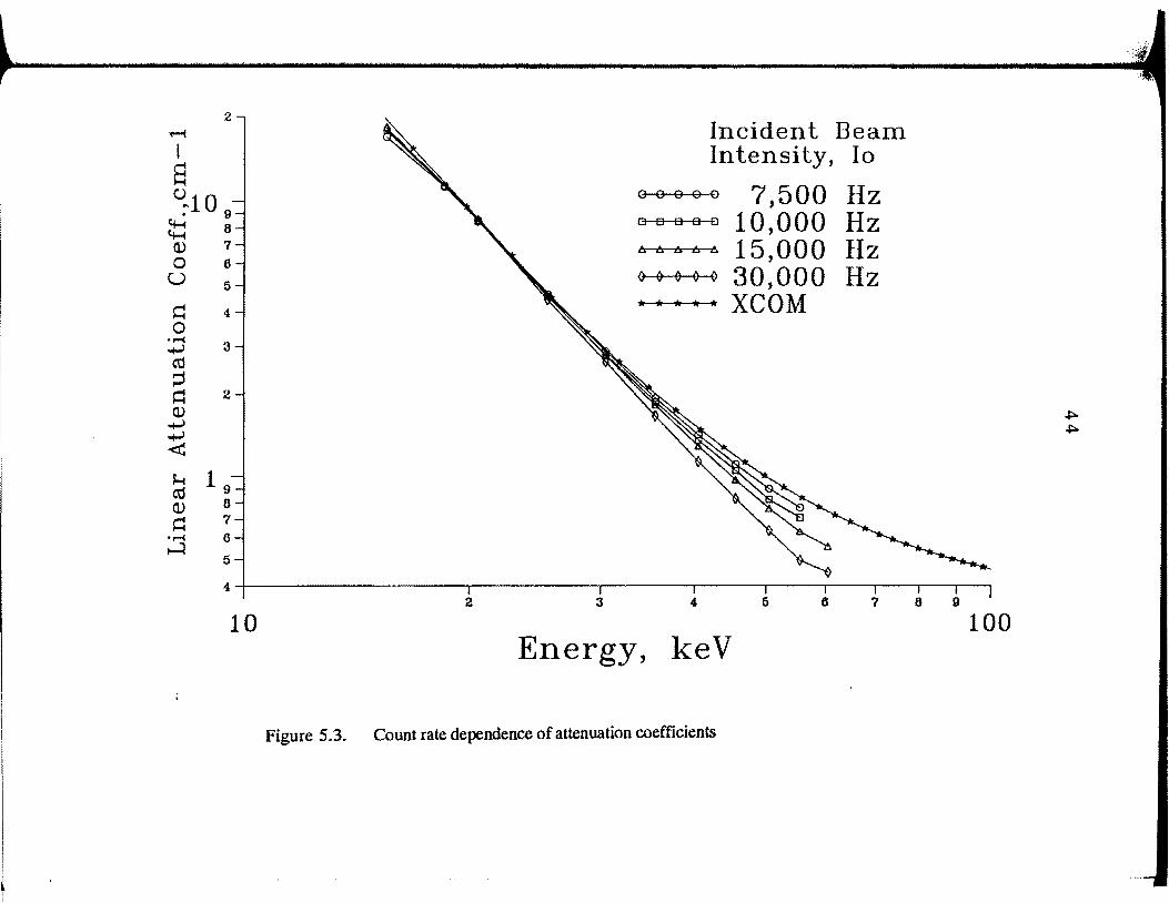
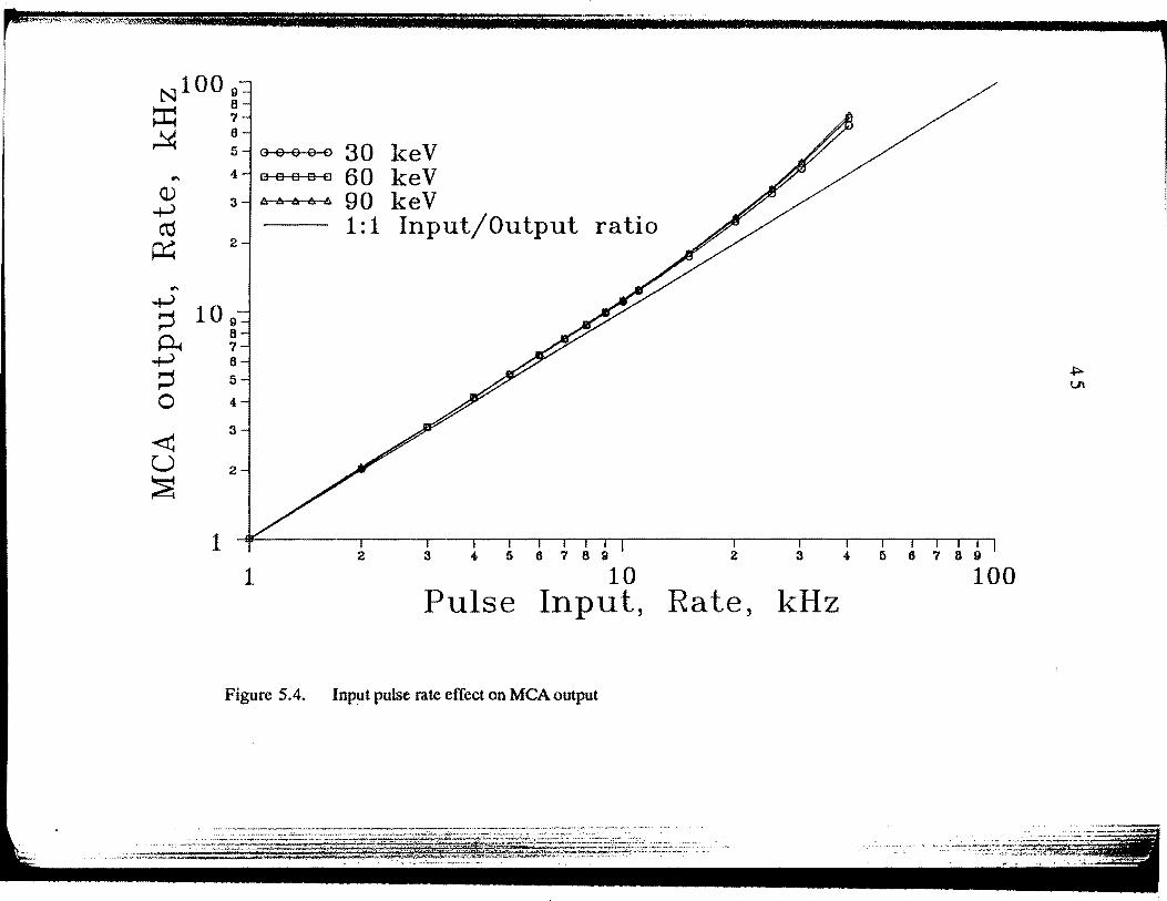
recorded for a preset live-time at an averaged count rate of 8 kHz or less. Figure 5.3 indicates

the measured attenuation coefficient is slightly count rate dependent. This observation was also

made by Gerward in his attenuation measurements [7]. Thus the detector system is operated in

the upper-most linear region of the detector count-rate curve, at about 8 kHz as shown in Fig.

5.4. The stability of the X-ray generator is monitored with the scanning program "MCA_2."

The results of our measurements did not indicate any fluctuations larger than those that can be

accounted for by the usual Poisson statistics. The background correction in the data was not

required in our attenuation measurements, because the background radiation is registered in the

incident and the transmitted beams. Therefore the background radiation will be subsequently

normalized as we take the transmission ratio of the beams.

2

2 3

Incident Beam Intensity, Io

ooooo 7,500 Hz osseo 10,000 Hz 6 6 o 6 c. 15,000 Hz o 0 0 0 o 30,000 Hz * * • • * XCOM

7 8 g

10 100 Energy, keV

Figure 5.3. Count rate dependence of attenuation coefficients

N100 9

~ ~ ~

6

"" ()..)

+> cO ~

2

"' +> 109 ~ 0-.

8 7

+> 6

~ 5

0 4

~ 3

u 2

~

1 1

30 keV 60 keV 90 keV 1:1 Input/Output ratio

5 6789 2 3 4 5 6769

10 100 Pulse Input, Rate, kHz

Figure 5.4. Input pulse rate effect on MCA output

46

5.2 Linear attenuation measurements for powders

There is an intrinsic difficulty in determining the attenuation coefficient of powders

because it is difficult to determine the thickness that should be used in calculating attenuation

coefficients. In this thesis work, we have developed a novel technique to measure the

attenuation coefficients for the powders. The powder is first ultrasonically packed into a glass

vial. The glass vial was thin and the diameter of the vial was uniform. A thin glass vial

attenuates less than a thick glass vial; thus one can maintain the high counting statistics in the

transmitted x-ray beam. We calculated the packed density of the powder by measuring the mass

of the powder in the vial and the volume of the vial. Then by taking an identical glass vial of

the same dimensions, we measured the incident and transmitted x-ray beams through the empty

and packed vials, respectively, to obtain the transmission ratio.

The major uncertainties for the linear attenuation coefficient measurements for the

powders come from the caliper measurements of the inner diameter of the vial and the packed­

density of the powder in the vial. The inner diameter of the vial is used to calculate the linear

attenuation coefficient of the packed powder. Thus we encounter the similar caliper thickness

uncertainty as we did for measuring the attenuation coefficients for solids. In addition to this,

we also have uncertainty due to the packed density measurements. It is also possible that the

packed density of the powder in the vial is non-uniform. Therefore care must be taken in

making the dimensional measurements for the linear attenuation calculations.

5.3 Experimental linear attenuation coefficient measurements

5.3.1 Graphite-epoxy composite

There is no published linear attenuation data for the composite IM-7 fibers. This is

because the individual fibers are only 5 microns in diameter. Therefore, we are not able to

measure the linear attenuation coefficients for the IM-7 fibers directly with the procedure

47

described in section 5.1. It is difficult to measure the total thickness of a bundle of fibers to

calculate the linear attenuation coefficients. Although we can generate the mass attenuation

coefficients for the IM-7 fiber based upon its chemical composition using XCOM, we do not

know the density of the IM-7 fibers; therefore we can not convert the mass attenuation

coefficients to the linear attenuation coefficients. Therefore, an indirect technique has to be used

to determine the linear attenuation coefficients for the IM-7 fibers. The indirect method uses the

linear attenuation coefficients of epoxy-resin and the beam attenuation of the characterized

Magnamite composite coupon to extrapolate the linear attenuation coefficients of the IM-7

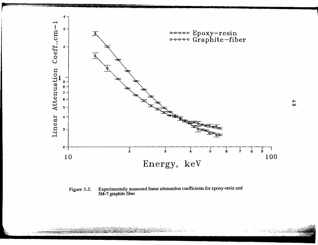
fibers, using Eq. 7. The extrapolated linear attenuation coefficients for the IM-7 fibers and the

measured linear attenuation coefficients for epoxy-resin are tabulated in Table 5.1, and they are

plotted in Fig. 5.5.

We were able to obtain three woven composite samples of IM-7, AS4 and Carbolon,

graphite fibers. IM-7 and AS4 are PAN-based graphite fibers, which differ with Carbolon,

which is a pitch-based graphite fiber, as defined based on manufacturing technique. The fibers

are essentially carbon based fibers with slightly different elemental compositions. The pitch­

based graphite fibers are derived from petroleum carbon polymer precursors, while the PAN­

based fibers are made from synthetic carbon polymer precursors. The fibers can differ in fiber

density, even among the PAN-based fibers. Although we are still unable to determine the

effective total thickness of the fiber in the bundles of woven fiber samples, we did measure the

effective-attenuation coefficients for the three graphite samples. This is a measure of the

transmission ratio divided by the thickness of the fiber bundle. The thickness includes the air

space between the woven fibers.

We determined the degree of confidence in our extrapolated linear attenuation

coefficient for IM-7 graphite fibers by dividing it by the effective-attenuation coefficients of

each of the three fiber samples. The slopes of the ratios, as a function of energy, would be

; lr~: ···~ jl: j . . ' :· ·' ,-{ ; !o f(;

~

I s c:; ... .

C+-4 C+-4 Q)

0 u ~ 0

.. I i J I ' tiiiPfiiiiiiTT ITit ) I Ill q I I I II B 1.1 II 1 I R

4

3 a 8 8 8 o Epoxy-resin o o o o a Graphite-fiber

2

•.-41 ..jooo) 9 Cd ::;; ~ Q)

..jooo)

..jooo)

< ~ Cd Q)

~ •.-4 ~

8

7

6

5

4

3

2 2 3

10 Energy, keV

Figure 5.5. Experimentally measured linear attenuation coefficients for epoxy-resin and IM-7 graphite fiber

,

100

49

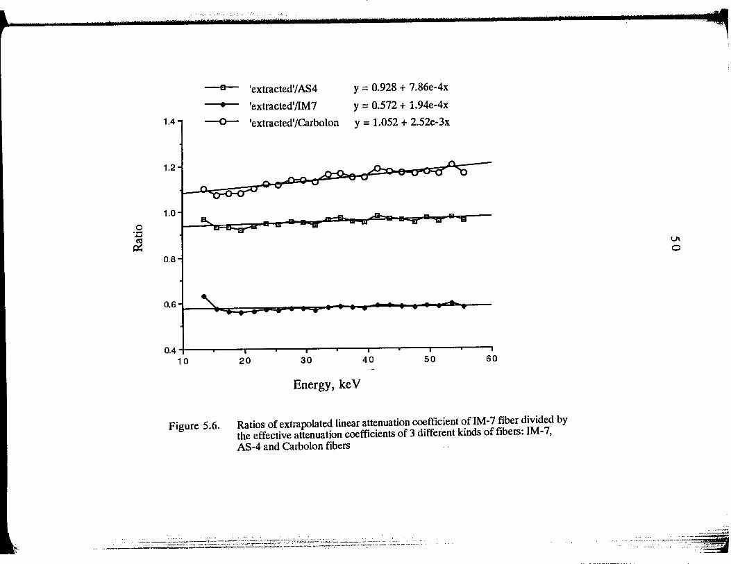
small if the chemical composition of the two materials is similar. This is because x-ray

attenuation is a function of the elemental composition of the compound, whereas, if the

composition of the materials is different, the slope of the ratio will be large. In Figure 5.6, we

see that the slope of the ratio obtained with IM-7 is the smallest. The slope obtained from AS4

is four times the ratio obtained with IM-7. Meanwhile, the slope of the ratio obtained with

Carbolon effective-attenuation is larger than the two previous slopes. This difference is

expected because the three fibers are made with two different manufacturing techniques. With

this analysis we have shown the confidence in our extracted IM-7 graphite fiber linear

Table 5.1. Experimentally measured linear attenuation values of epoxy-resin and graphite IM-7 fibers

ll ll 11 of uncertainty 11 of IM-7 uncertainty

Energy epoxy-resm for epoxy-resin fibers for IM-7 fibers (keY) (cm-1) a (%) * (cm-1) a (%) * 13.5 2.72 4.9 1.64 6.8 15.5 2.01 1.8 1.23 6.8 17.5 1.49 7.1 0.960 2.0 19.5 1.155 0.6 0.773 0.6 21.5 0.915 0.2 0.659 0.4 23.5 0.753 0.2 0.580 0.2 25.5 0.639 0.2 0.516 1.9 27.5 0.555 0.3 0.478 0.8 29.5 0.491 0.3 0.442 0.0 31.5 0.449 0.5 0.412 1.8 33.5 0.411 1.0 0.400 0.1 35.5 0.378 0.8 0.385 0.8 37.5 0.359 0.3 0.368 2.2 39.5 0.342 0.4 0.354 0.6 41.5 0.318 2.2 0.354 2.8 43.5 0.301 2.0 0.344 4.4 45.5 0.297 2.2 0.334 1.1 47.5 0.291 1.2 0.325 1.0 49.5 0.275 2.2 0.325 3.7 51.5 0.275 0.8 0.316 1.3 53.5 0.262 1.3 0.320 4.0 55.5 0.263 0.9 0.307 2.0

a. number of experimental measurements n = 3. * one standard deviation

;.

'·'

.;:

; . { ~

:ti ~ '; ! f

''1 . !! ! ·I·

. ljl ,·. t

-:lrL

~~t ·--:l.R 'h1'f: i ~~- i ,r'j' l1l' d1r • flh r ' .. i:

:ll \ ·I L

!I' I \

'I I \ i I

0 ·-...... ~ ~

1.4

1.0

0.8

···.··-'·;''

• 'extracted'/ AS4

'extracted'/IM7

y = 0.928 + 7.86e-4x

y = 0.572 + 1.94e-4x

--o-- 'extracted'/Carbolon y = 1.052 + 2.52e-3x

0.4 ;----.----,r---r---,------~---.----r--~--.

10 20 30 40 50 60

Energy, keY

Figure 5.6. Ratios of extrapolated linear attenuation coefficient of IM-7 fiber divided by the effective attenuation coefficients of 3 different kinds of fibers: IM-7, AS-4 and Carbolon fibers

_. __ .. .. :· -- --··-:-:-:.~= -. . -_ -=~-=---::::::.:::-..:::.:-~~~=-::-:::::- ·--;··::.;..:.,~~:;:-<!.:.~~~::~::::·:;::.:.:-:~~;:;~-::·:_.;~~;_~-i-...::.., _ _:_...:_.~------: , ,.._, ,. . ....,. .. ..._,.,,.,.,.,_,,._~_.. .... ,..._, __ ~·---<"":":":'"'"'""4-~·-~,...._...r_~~·-·--..,... -~---~-··• • - -•

I.J\

0

.... ----- ... ---~

-·~--~<.:--·~-;_-~:s~~~

51

attenuation coefficients.

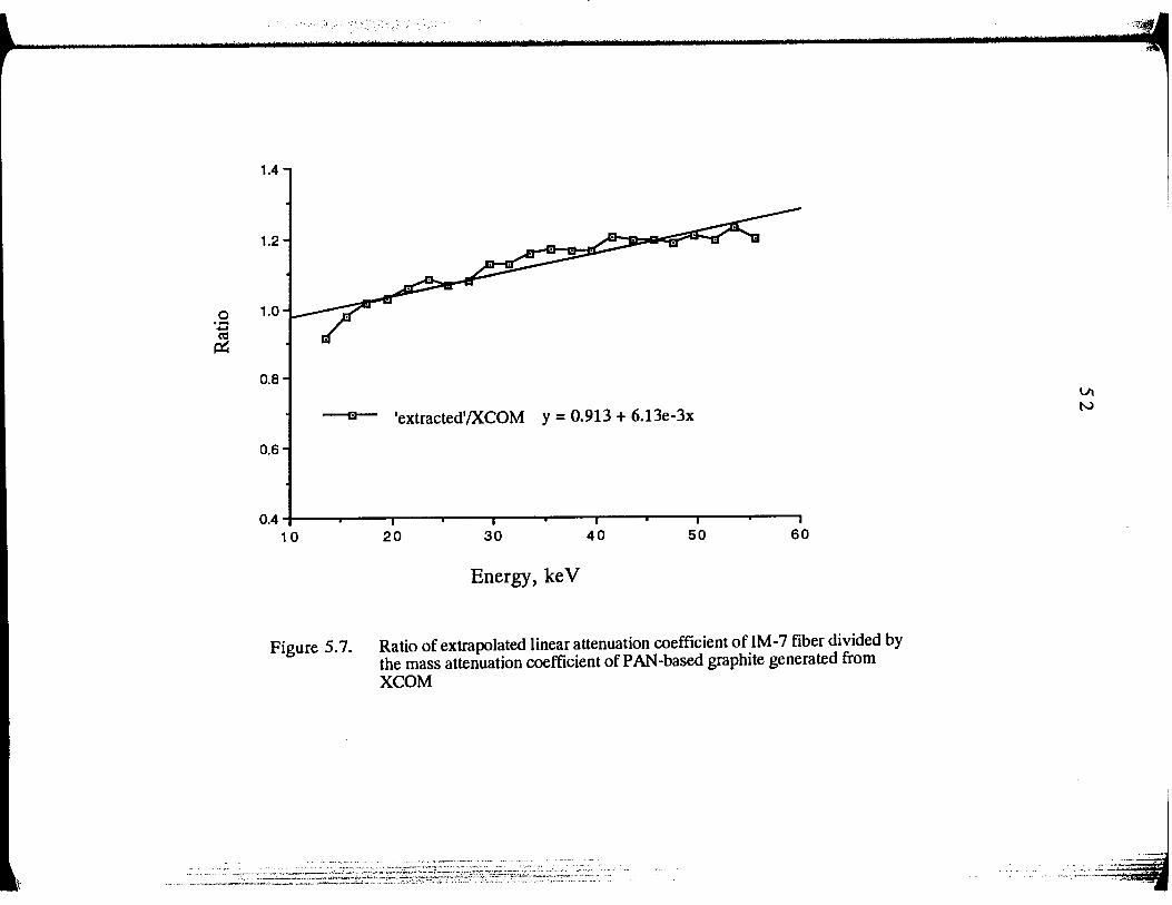
We generated the mass attenuation coefficients for a PAN-based graphite fiber from

XCOM using the chemical compositions given by International Encyclopedia of Composites

[13]. We discovered that the mass attenuation coefficient slope, from XCOM, did not agree

with the slope in the extrapolated attenuation coefficient slope. The slope of the ratio obtained

from dividing the extrapolated coefficients by XCOM coefficients are too large to show

agreement between the two attenuation slopes (see Fig. 5.7). This further demonstrated that it

is necessary to measure one's own linear attenuation coefficients for a material.

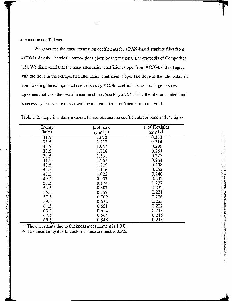
Table 5.2. Experimentally measured linear attenuation coefficients for bone and Plexiglas

Energy 11 of bone 11 of Plexiglas (keY) (cm-1) a (cm-1) b 31.5 2.670 0.333 33.5 2.277 0.314 35.5 1.967 0.296 37.5 1.726 0.284 39.5 1.531 0.275 41.5 1.367 0.264 43.5 1.229 0.258 45.5 1.116 0.252 47.5 1.022 0.246 49.5 0.937 0.242 51.5 0.874 0.237 53.5 0.807 0.232 55.5 0.757 0.231 57.5 0.709 0.226 59.5 0.672 0.223 61.5 0.651 0.222 63.5 0.614 0.218 67.5 0.564 0.215 69.5 0.548 0.213

a. The uncertainty due to thickness measurement is 1.0%. b. The uncertainty due to thickness measurement is 0.3%.

i' f ~

F ~ -~ . j ·;

H~ -;_.~ .;!!·· -; ,-(; 1-: '\i'

1.4

1.2

0 1.0 ·­..... ~ ~

0.8

'extracted'/XCOM y = 0.913 + 6.13e-3x

0.6

0.4 +----T"--r-----r----,..---,-----r----r--~-....... 10 20 30 40 50 60

Energy, keY

Figure 5. 7. Ratio of extrapolated linear attenuation coefficient of IM-7 fiber divided by the mass attenuation coefficient of PAN-based graphite generated from XCOM

'-- - ... -~~---~- -·-~--·· ·~·-- . --- ·- -

----~-::~-~~~~:::-~~~-=-==:~:-:~~~~?~iT;~~E~:~~~--~·~:~-~~~:S~~~~~.s::·ji~~~~;:::~=-~ · .~.::·~~:~~ ·=-

53

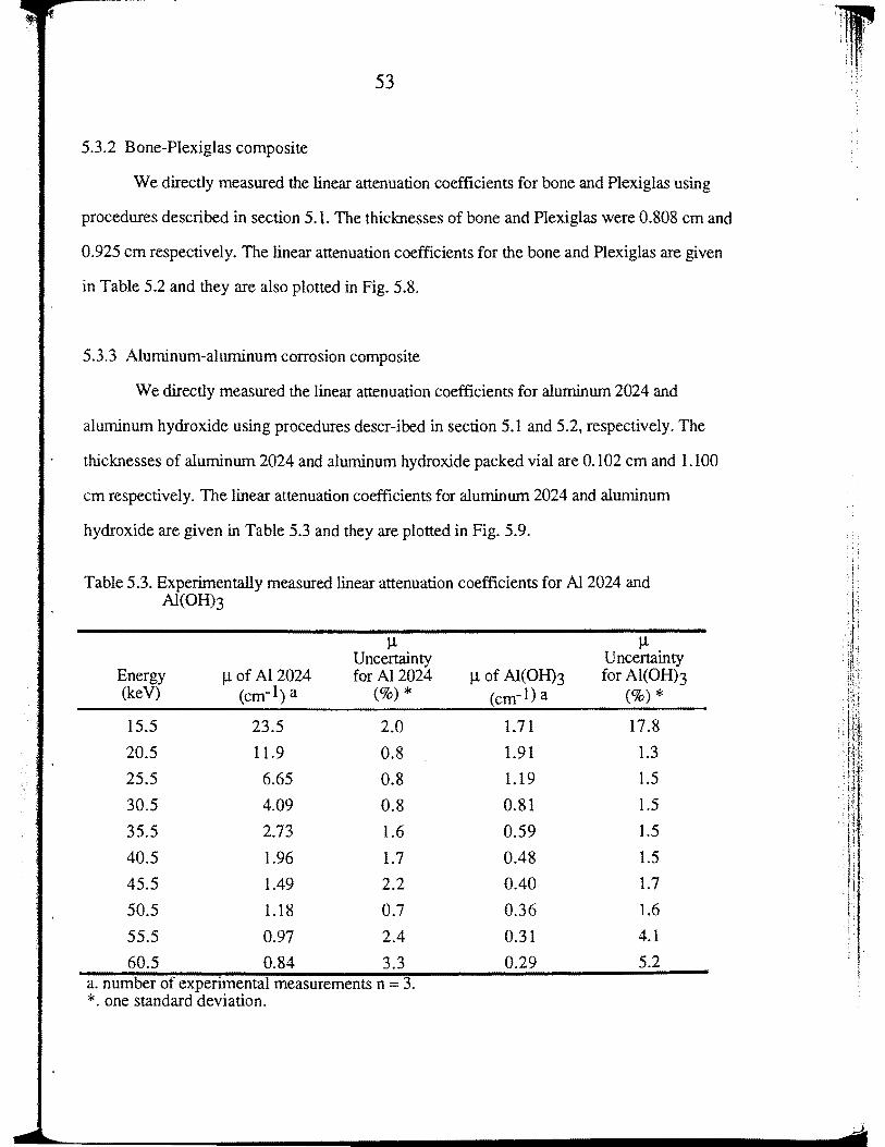
5.3.2 Bone-Plexiglas composite

We directly measured the linear attenuation coefficients for bone and Plexiglas using

procedures described in section 5.1. The thicknesses of bone and Plexiglas were 0.808 em and

0.925 em respectively. The linear attenuation coefficients for the bone and Plexiglas are given

in Table 5.2 and they are also plotted in Fig. 5.8.

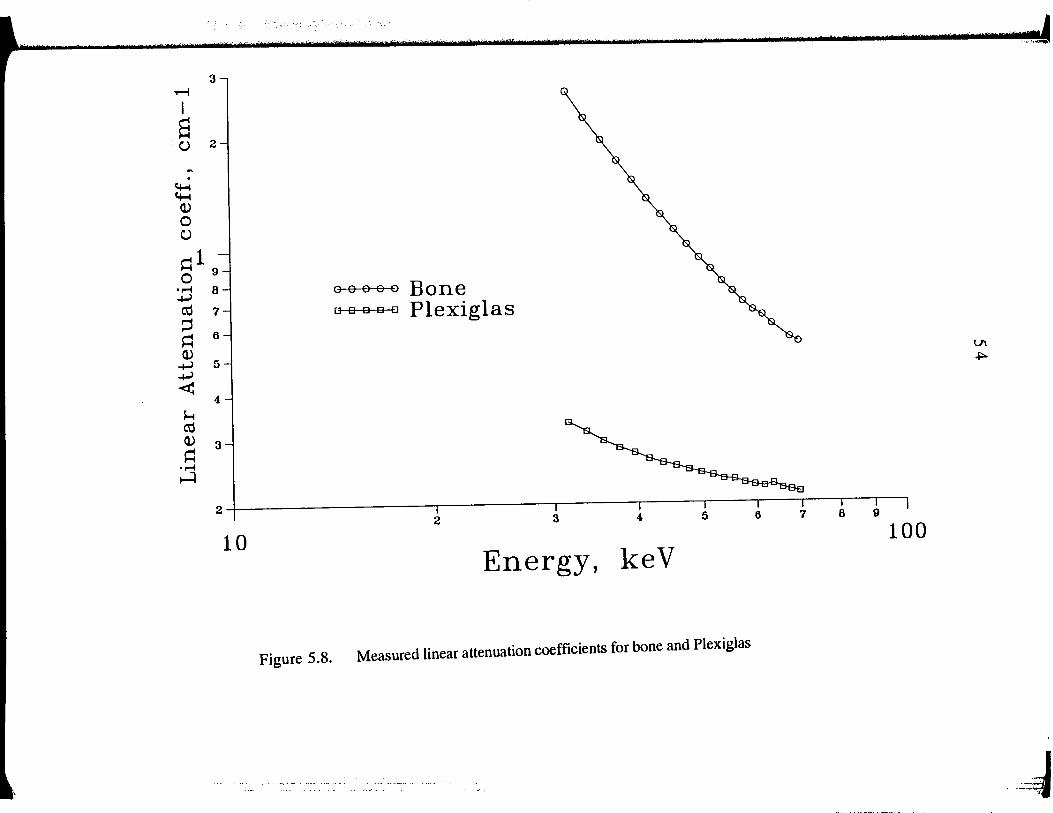
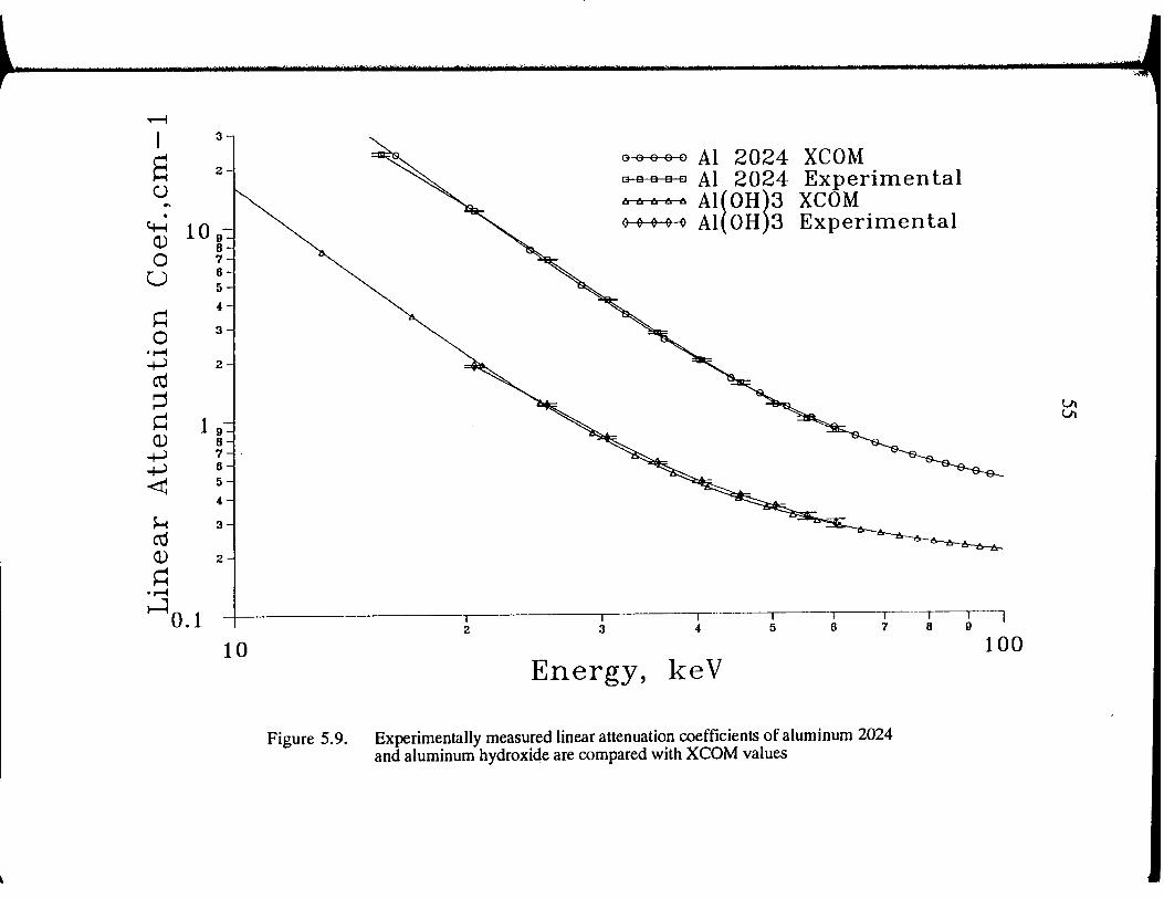
5.3.3 Aluminum-aluminum corrosion composite

We directly measured the linear attenuation coefficients for aluminum 2024 and

aluminum hydroxide using procedures descr-ibed in section 5.1 and 5.2, respectively. The

thicknesses of aluminum 2024 and aluminum hydroxide packed vial are 0.102 em and 1.100

em respectively. The linear attenuation coefficients for aluminum 2024 and aluminum

hydroxide are given in Table 5.3 and they are plotted in Fig. 5.9.

Table 5.3. Experimentally measured linear attenuation coefficients for A12024 and Al(OH)3

)l )l Uncertainty Uncertainty

Energy Jl of Al2024 for Al2024 Jl of Al(OH)3 for Al(OH)3 (keV) (cm-1) a (%) * (cm-1) a (%) * 15.5 23.5 2.0 1.71 17.8

20.5 11.9 0.8 1.91 1.3

25.5 6.65 0.8 1.19 1.5

30.5 4.09 0.8 0.81 1.5

35.5 2.73 1.6 0.59 1.5

40.5 1.96 1.7 0.48 1.5

45.5 1.49 2.2 0.40 1.7

50.5 1.18 0.7 0.36 1.6

55.5 0.97 2.4 0.31 4.1

60.5 0.84 3.3 0.29 5.2 a. number of experimental measurements n = 3. *. one standard deviation.

3 .-i

I s () 2

. C+--4 C+--4 Q)

0 ()

~1 0 9 ·~ 8 ~ cd 7 :;j ~ 6 Q) ~ 5 ~

< 4

3

o o o o o Bone o o o o o Plexiglas

2 ' 3

100 10 Energy, keV

Figure 5.8. Measured linear attenuation coefficients for bone and Plexiglas

.. ~

~

I s ()

10 2

0 0 0 0 0

08880

0 & & & 0

3

AI 2024 XCOM AI 2024 Experimental AI( OH)3 XCOM AI( OH)3 Experimental

Energy, keV

Figure 5.9. Experimentally measured linear attenuation coefficients of aluminum 2024 and aluminum hydroxide are compared with XCOM values

56

6. RESULTS AND DISCUSSIONS

n.l Introduction

As mentioned in the Section 2, we need to optimize the choice of energy-pair used in

this energy-dispersive technique. Since there are three composite systems in this thesis, we

need three different optimum energy-pairs for the three studies. The derived error-propagation

expressions given by Eq. 14 are used to predict the optimum energy-pairs. The error

propagation expression is used to determine the optimum energy-pair for each composite

system to give the least uncertainty in our thickness, or density, measurements.

For the section that follows, all the experimental thickness, and density, measurements

will be compared to the caliper measured thicknesses, and densities. All measurement

deviations presented in the tables are determined by comparing the measured values to the

values determined by a caliper. The deviations are given as percentages of the caliper value.

Discussion of the results are presented in each section for the three composite studies.

n.2 Graphite-epoxy composite measurements

6.2.1 Optimization study

The prediction model for determining the optimum energy-pair uses the error­

propagation expressions given in Eq. 14. To realistically predict the experimental uncertainties

in the thickness measurements, we used experimental linear attenuation coefficients and

experimental attenuation uncertainties given in Table 5.1. The beam transmission uncertainties

are not present in our prediction models, because all our experimental counting statistics are

high, on the order of several millions of counts. Therefore the beam transmission uncertainties

are small and they can be ignored in Eq. 14.

57

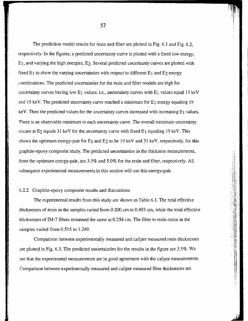
The prediction model results for resin and fiber are plotted in Fig. 6.1 and Fig. 6.2,

respectively. In the figures, a predicted uncertainty curve is plotted with a fixed low energy,

E I, and varying the high energies, E2. Several predicted uncertainty curves are plotted with

fixed E I to show the varying uncertainties with respect to different E 1 and E 2 energy

combinations. The predicted uncertainties for the resin and fiber models are high for

uncertainty curves having low EI values; i.e., uncertainty curves with E1 values equal 13 keY

and 15 keY. The predicted uncertainty curve reached a minimum forE 1 energy equaling 19

keY. Then the predicted values for the uncertainty curves increased with increasing E 1 values.

There is an observable minimum in each uncertainty curve. The overall minimum uncertainty

occurs at E2 equals 31 keY for the uncertainty curve with fixed E 1 equaling 19 keY. This

shows the optimum energy-pair for E 1 and E 2 to be 19 keY and 31 keY, respectively, for this

graphite-epoxy composite study. The predicted uncertainties in the thickness measurements,

from the optimum energy-pair, are 3.5% and 5.0% for the resin and fiber, respectively. All

subsequent experimental measurements in this section will use this energy-pair.

6.2.2 Graphite-epoxy composite results and discussions

The experimental results from this study are shown in Table 6.1. The total effective

thicknesses of resin in the samples varied from 0.200 em to 0.493 em, while the total effective

thicknesses of IM-7 fibers remained the same at 0.254 em. The fiber to resin ratios in the

samples varied from 0.515 to 1.249.

Comparison between experimentally measured and caliper measured resin thicknesses

are plotted in Fig. 6.3. The predicted uncertainties for the results in the figure are 3.5%. We

see that the experimental measurements are in good agreement with the caliper measurements.

Comparison between experimentally measured and caliper measured fiber thicknesses are

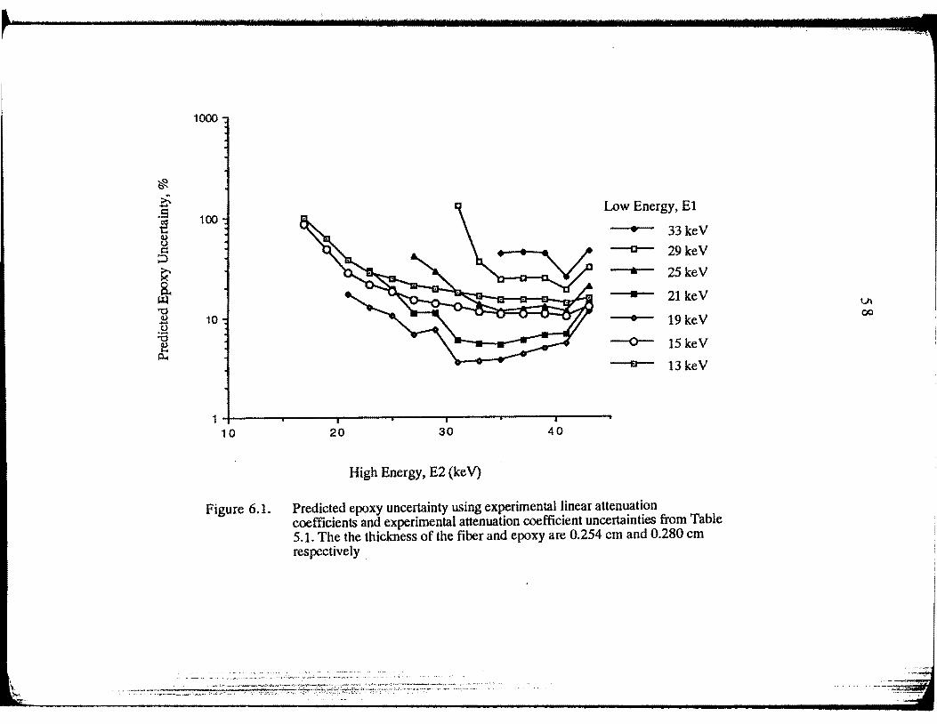
* ~ .5 t! CL) 0 c

;:J

~ &

r.l.l "0

CL) ..... 0 :a e p.,

~000

Low Energy, E1 ~00

• 33keV c 29keV

* 25keV

• 21 keV

~0 19keV

--o-- 15 keV

I'll 13keV

10 20 30 40

High Energy, E2 (keV)

Figure 6.1. Predicted epoxy uncertainty using experimental linear attenuation coefficients and experimental attenuation coefficient uncertainties from Table 5.1. The the thickness of the fiber and epoxy are 0.254 em and 0.280 em respectively .

V\ 00

~

i-c: ·~

<1) u c:

;;::J ..... <1)

:-9 ~ '0

<1) ..... .~ '0

<1) ..... p..

1000

Low Energy, E1

33keY 100 29keY

,. 25keY

• 21 keY

0 19 keY

10 .. 15 keY

1!1 13keY

10

High Energy, E2 (keY)

Figure 6.2. Predicted graphite fiber uncertainty using experimental linear attenuation coefficients and experimental attenuation coefficient uncertainties given in Table 5.1. The thickness of fiber and epoxy are 0.254 em and 0.280 em

respectively

VI

\0

. ··--- ----------------------

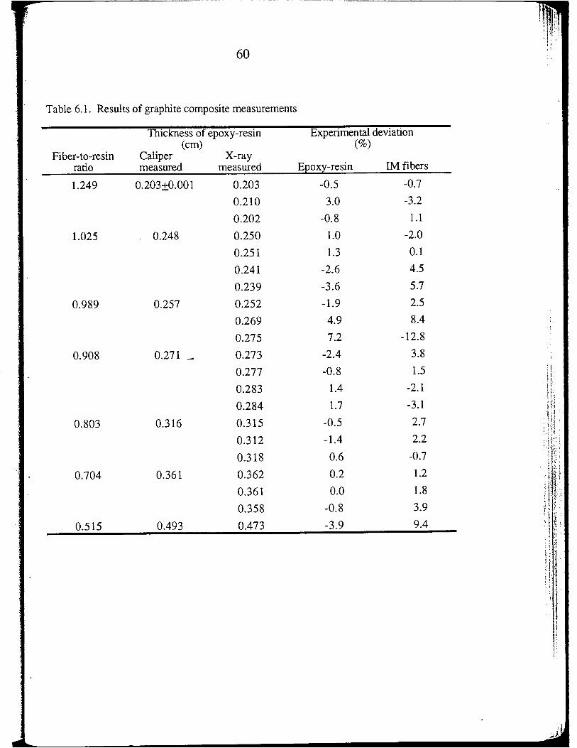
60

Table 6.1. Results of graphite composite measurements

Fiber-to-resin ratio

1.249

1.025

0.989

0.908

0.803

0.704

0.515

Thickness of epoxy-resin (em)

Caliper measured

0.203±0.00 1

0.248

0.257

0.271 --

0.316

0.361

0.493

X-ray measured

0.203

0.210

0.202

0.250

0.251

0.241

0.239

0.252

0.269

0.275

0.273

0.277

0.283

0.284

0.315

0.312

0.318

0.362

0.361

0.358

0.473

Experimental deviation (%)

Epoxy-resin

-0.5

3.0

-0.8

1.0

1.3 -2.6

-3.6

-1.9 4.9

7.2

-2.4

-0.8

1.4 1.7

-0.5

-1.4 0.6

0.2

0.0

-0.8

-3.9

IM fibers

-0.7

-3.2

1.1

-2.0

0.1

4.5

5.7

2.5

8.4

-12.8

3.8

1.5 -2.1

-3.1

2.7

2.2

-0.7

1.2

1.8 3.9 9.4

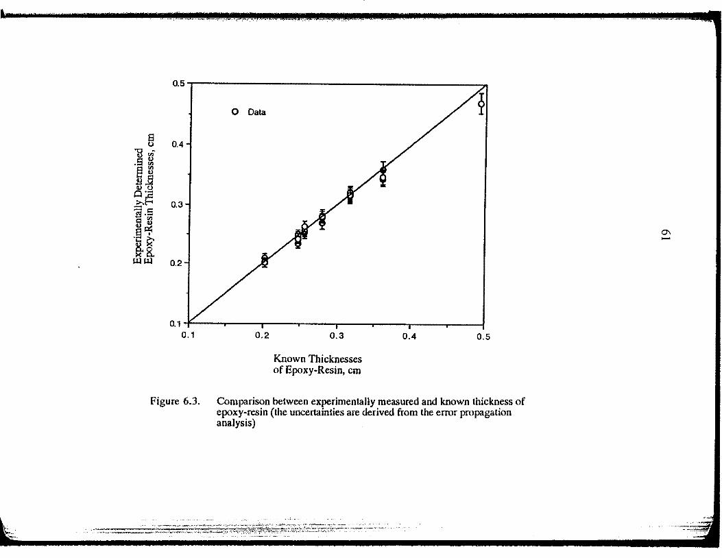
E1 13 VJ~ .!3 ~ § ~ ~~ o·->.~

:::::c: .S·-c: VJ u u

-~~ ~8.

1-QI-Q

0.5

0 Data

0.4

0.3

0.2

Q1~----~----~----r-----r---~----~----~----~ 0.1 0.2 0.3

Known Thicknesses of Epoxy-Resin, em

0.4 0.5

Figure 6.3. Comparison between experimentally measured and known thickness of epoxy-resin (the uncertainties are derived from the error propagation analysis)

0\ -

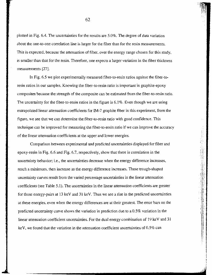
62

plotted in Fig. 6.4. The uncertainties for the results are 5.0%. The degree of data variation

about the one-to-one correlation line is larger for the fiber than for the resin measurements.

This is expected, because the attenuation of fiber. over the energy range chosen for this study,

is smaller than that for the resin. Therefore, one expects a larger variation in the fiber thickness

measurements [27].

In Fig. 6.5 we plot experimentally measured fiber-to-resin ratios against the fiber-to-

resin ratios in our samples. Knowing the fiber-to-resin ratio is important in graphite-epoxy

composites because the strength of the composite can be estimated from the fiber-to-resin ratio.

The uncertainty for the fiber-to-resin ratios in the figure is 6.1 %. Even though we are using

extrapolated linear attenuation coefficients for IM-7 graphite fiber in this experiment, from the

figure, we see that we can determine the fiber-to-resin ratio with good confidence. This

technique can be improved for measuring the fiber-to-resin ratio if we can improve the accuracy

of the linear attenuation coefficients at the upper and lower energies.

Comparison between experimental and predicted uncertainties displayed for fiber and

epoxy-resin in Fig. 6.6 and Fig. 6.7, respectively, show that there is correlation in the

uncertainty behavior; i.e., the uncertainties decrease when the energy difference increases,

reach a minimum, then increase as the energy difference increases. These trough-shaped

uncertainty curves result from the varied percentage uncertainties in the linear attenuation

coefficients (see Table 5.1). The uncertainties in the linear attenuation coefficients are greater

for those energy-pairs at 13 ke V and 31 ke V. Thus we see a rise in the predicted uncertainties

at these energies, even when the energy differences are at their greatest. The error bars on the

predicted uncertainty curve shows the variation in prediction due to a 0.5% variation in the

linear attenuation coefficient uncertainties. For the dual energy combination of 19 keY and 31

ke V, we found that the variation in the attenuation coefficient uncertainties of 0.5% can

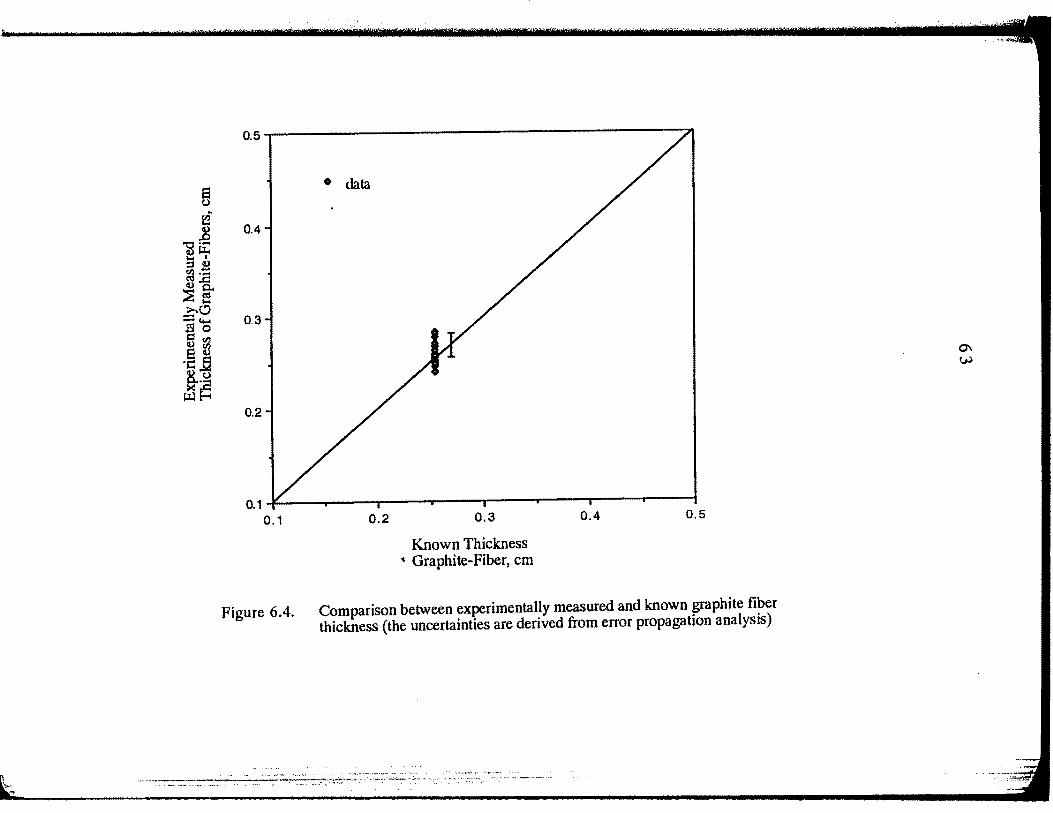
§ li tU

.D 1HZ

.... I ::I tU ~-~ <U..c:: ~a. e ~c.? -(+.I

!9o s:l{l) tU {I)

StU ·c J2 §.:E ~.LH-~

0.5

• data

0.4

0.3

0.2

0.1 +--..------,----.----.---....-----.:-----r---1 0.1 0.2 0.3

Known Thickness • Graphite-Fiber, em

0.4 0.5

Figure 6.4. Comparison between experimentally measured and known graphite fiber thickness (the uncertainties are derived from error propagation analysis)

0\ v.>

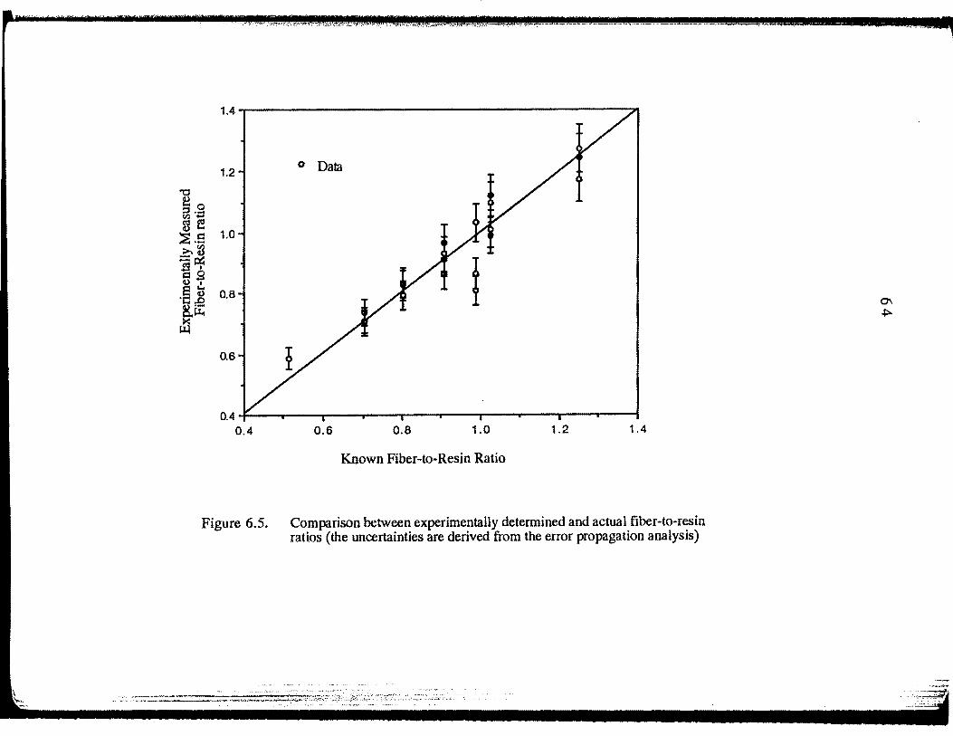
1.4~-----------------------------------------------

0 Data 1.2

"'C

~0 :::s .... fll ....

a:s e 1.0 ::E .s

>.~ ;:p:::; S• s:l.9 Cl,),

.~] 0.8

~ji: IJ;.l

0.6

0.4~---r----r---~--~--~~--~--~----r---,---~

0.4 0.6 0.8 1.0 1.2 1.4 Known Fiber-to-Resin Ratio

Figure 6.5. Comparison between experimentally determined and actual fiber-to-resin ratios (the uncertainties are derived from the error propagation analysis)

C1\ ~

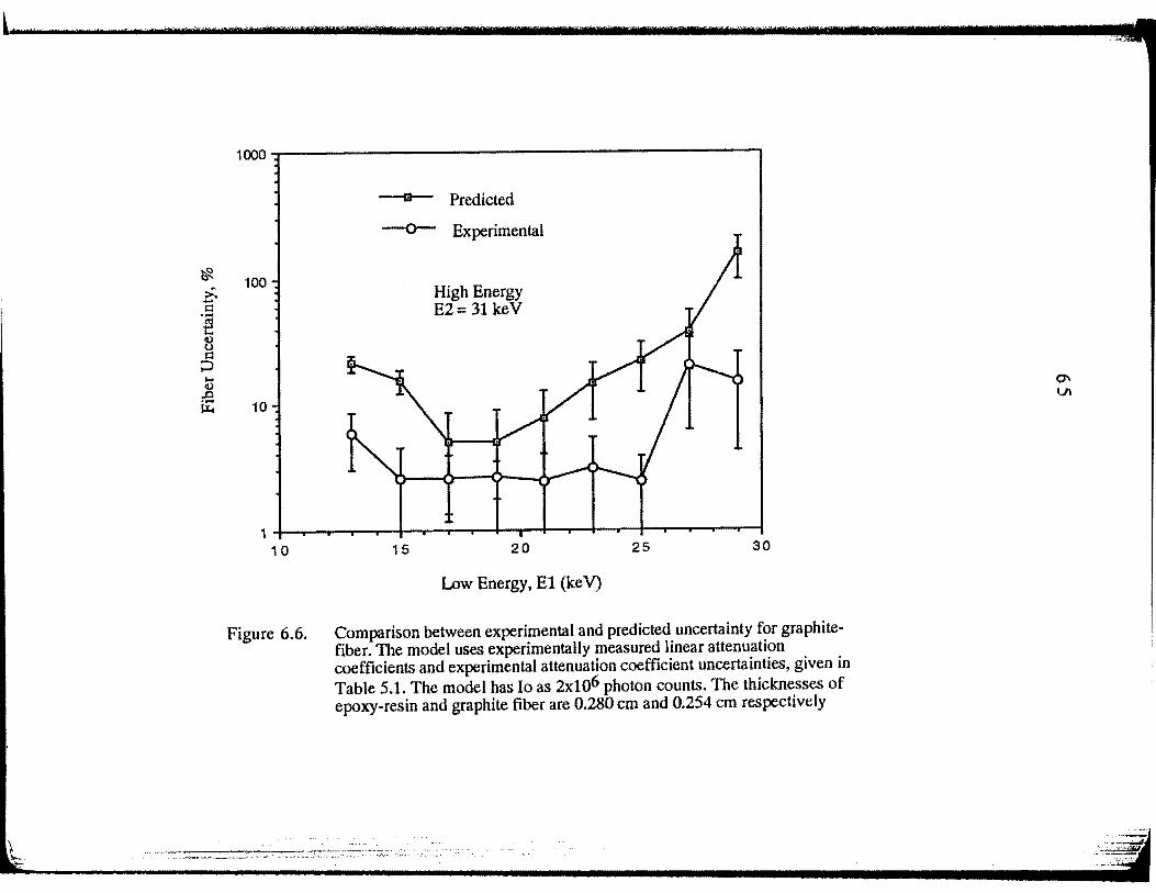
~ >: -s:: "! 8 s:: ;:J .... q.)

..0 ·-~

1000

-- Predicted

-o- Experimental

100 High Energy E2= 31 keV

10

10 15 20 25 30

Low Energy, El (keV)

Figure 6.6. Comparison between experimental and predicted uncertainty for graphite­fiber. The model uses experimentally measured linear attenuation coefficients and experimental attenuation coefficient uncertainties, given in Table 5.1. The model has Io as 2x106 photon counts. The thicknesses of epoxy-resin and graphite fiber are 0.280 em and 0.254 em respectively

0"1 V'l

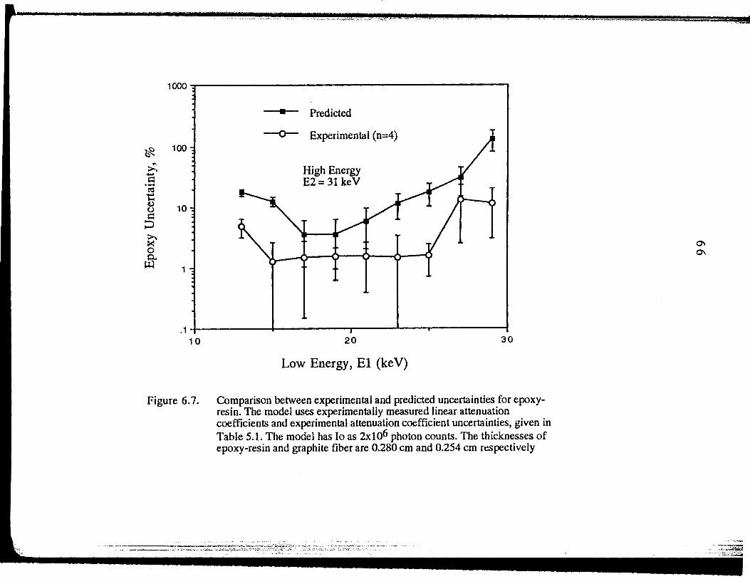
1000

• Predicted

-o- Experimental (n=4)

~ 100

~ High Energy ...... ~ E2= 31 keV ·-ca ...... .... Q.)

10 u ~

;:::> >. ~ 0

& 1

.14---------~~---------r----~~--~---------1 10

Figure 6.7.

20 30

Low Energy, El (ke V)

Comparison between experimental and predicted uncertainties for epoxy­resin. The model uses experimentally measured linear attenuation coefficients and experimental attenuation coefficient uncertainties, given in Table 5.1. The model has Io as 2xto6 photon counts. The thicknesses of epoxy-resin and graphite fiber are 0.280 em and 0.254 em respectively

"' "'

-

67

contribute up to 1.7% variation in the predicted uncertainty for the thickness measurements.

This can explain the discrepancies between predicted and experimental uncertainties.

11.3 Bone-Plexiglas composite measurements

6.3.1 Optimization study

The prediction model for determining the optimum energy-pair uses experimental linear

attenuation coefficients given in Table 5.3. The beam transmission uncertainties are not

significant in our predictions. The uncertainties for the bone and Plexiglas linear attenuation

coefficients are determined using the error-propagation analysis using Eq. 14. The uncertainties

in the bone and Plexiglas attenuation coefficients are related to the thickness uncertainties in the

caliper measurements used in the linear attenuation calculation. The uncertainties for the bone

and Plexiglas coefficients are 1.0% and 0.3% respectively for all the energy measurements.

The predictions for determining the optimum energy-pair for bone and Plexiglas are

shown in Fig. 6.8 and Fig. 6.9 respectively. The optimum energy-pair in the figures gives the

least predicted percentage uncertainties. For this bone-Plexiglas composite system, the

optimum energy-pair is 31 ke V for the low-energy, E 1, and 61 ke V for the high-energy, E2.

All subsequent experimental measurements in this section used this energy-pair.

From the two figures mentioned above, the predicted percentage uncertainty curves

converge as the E2 value increases. In fact, the predicted percentage bone uncertainties level off

on the uncertainty curve with fixed low-energy value, E 1, equaling 31 ke V. This demonstrates

that choosing energies that are farther apart than those energies used in this model will not

significantly improve the uncertainty in the thickness measurements. Instead, to improve the

experimental measurements, one should concentrate on improving the uncertainties in the linear

attenuation coefficient measurements. We found the uncertainties in the linear attenuation

coefficients strongly affect the accuracy of the thickness and density calculations [28].

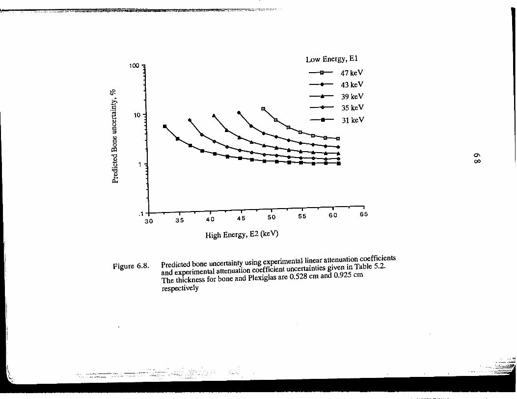
Low Energy, El 100

m 47keV

• 43keV ~ .. 39keV c c: -~ 10

35keV

cl.) C)

31 keV c: ::s g 0

I:Q

13 ..... 1 C) :.a

cl.) .... ~

30 35 40

High Energy, E2 (keV)

Figure 6.8. Predicted bone uncertainty using experimental linear attenuation coefficients and experimental attenuation coefficient uncertainties given in Table 5.2. The thickness for bone and Plexiglas are 0.528 em and 0.925 em

respectively

---------"~--------...,..---------·----

0\ 00

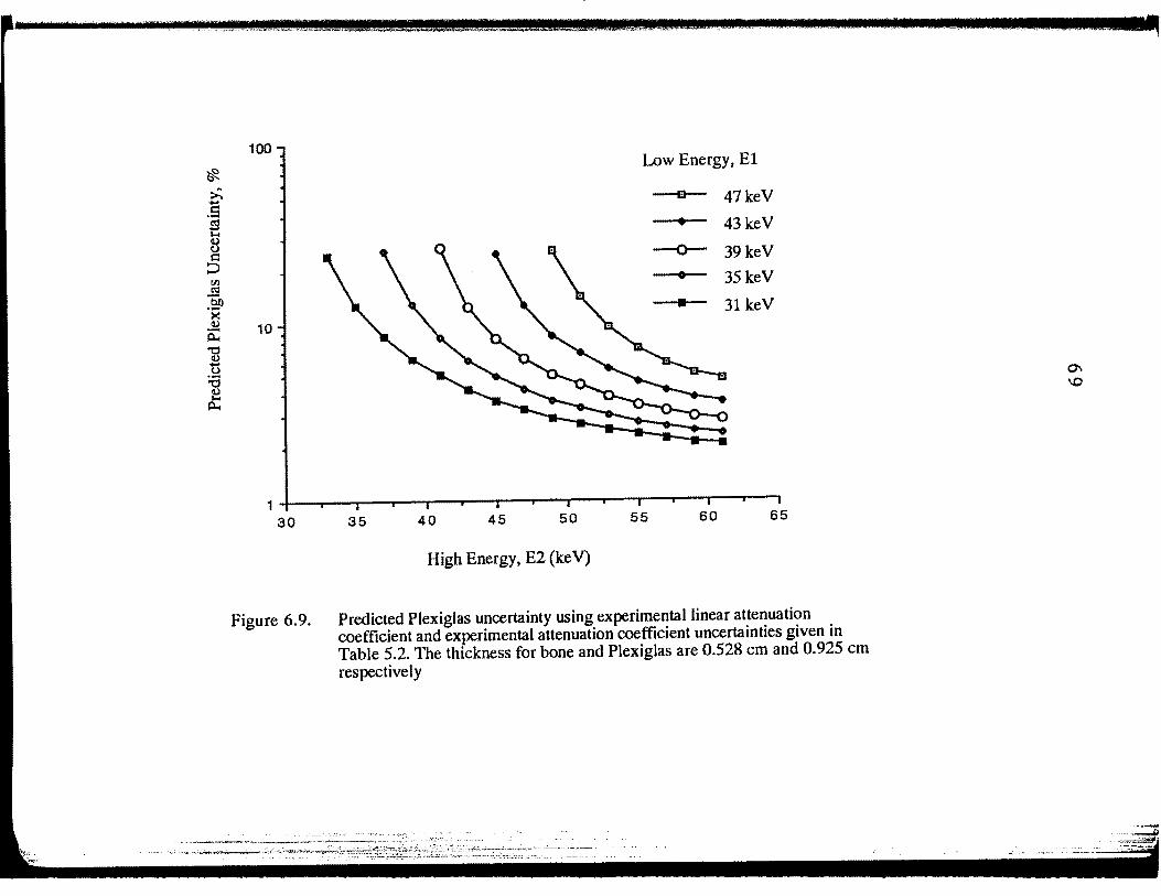
I •

~ :>. -c: -~ 8 c: ~

<1.1 Cl:l

bn ">< ~ p..

1S -0

:a ~ ~ p..

I!! !I!!!!!!! !II

100 Low Energy, El

--e- 47keV

• 43keV

-o- 39keV

• 35keV

• 31 keV

10

1 4---~~r-~--~--~--r-~---r--~--~~r-~---r--,

30 35 40 45 50 55 60 65

High Energy, E2 (ke V)

Figure 6.9. Predicted Plexiglas uncertainty using experimental linear attenuation coefficient and experimental attenuation coefficient uncertainties given in Table 5.2. The thickness for bone and Plexiglas are 0.528 em and 0.925 em respectively

0\ \C

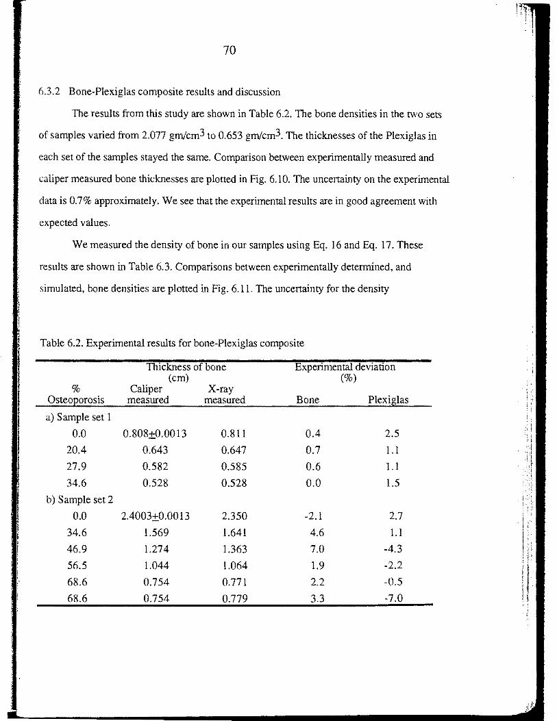
70

6.3.2 Bone-Plexiglas composite results and discussion

The results from this study are shown in Table 6.2. The bone densities in the two sets

of samples varied from 2.077 gm/cm3 to 0.653 gm/cm3. The thicknesses of the Plexiglas in

each set of the samples stayed the same. Comparison between experimentally measured and

caliper measured bone thicknesses are plotted in Fig. 6.1 0. The uncertainty on the experimental

data is 0.7% approximately. We see that the experimental results are in good agreement with

expected values.

We measured the density of bone in our samples using Eq. 16 and Eq. 17. These

results are shown in Table 6.3. Comparisons between experimentally determined, and

simulated, bone densities are plotted in Fig. 6.11. The uncertainty for the density

Table 6.2. Experimental results for bone-Plexiglas composite

Thickness of bone Experimental deviation (em) (%)

% Caliper X-ray OsteoEorosis measured measured Bone Plexiglas

a) Sample set 1

0.0 0.808±0.0013 0.811 0.4 2.5

20.4 0.643 0.647 0.7 1.1

27.9 0.582 0.585 0.6 1.1

34.6 0.528 0.528 0.0 1.5

b) Sample set 2

0.0 2.4003±0. 00 13 2.350 -2.1 2.7

34.6 1.569 l.641 4.6 1.1

46.9 1.274 1.363 7.0 -4.3

56.5 1.044 1.064 1.9 -2.2

68.6 0.754 0.771 2.2 -0.5

68.6 0.754 0.779 3.3 -7.0

i I ! I l! ' l

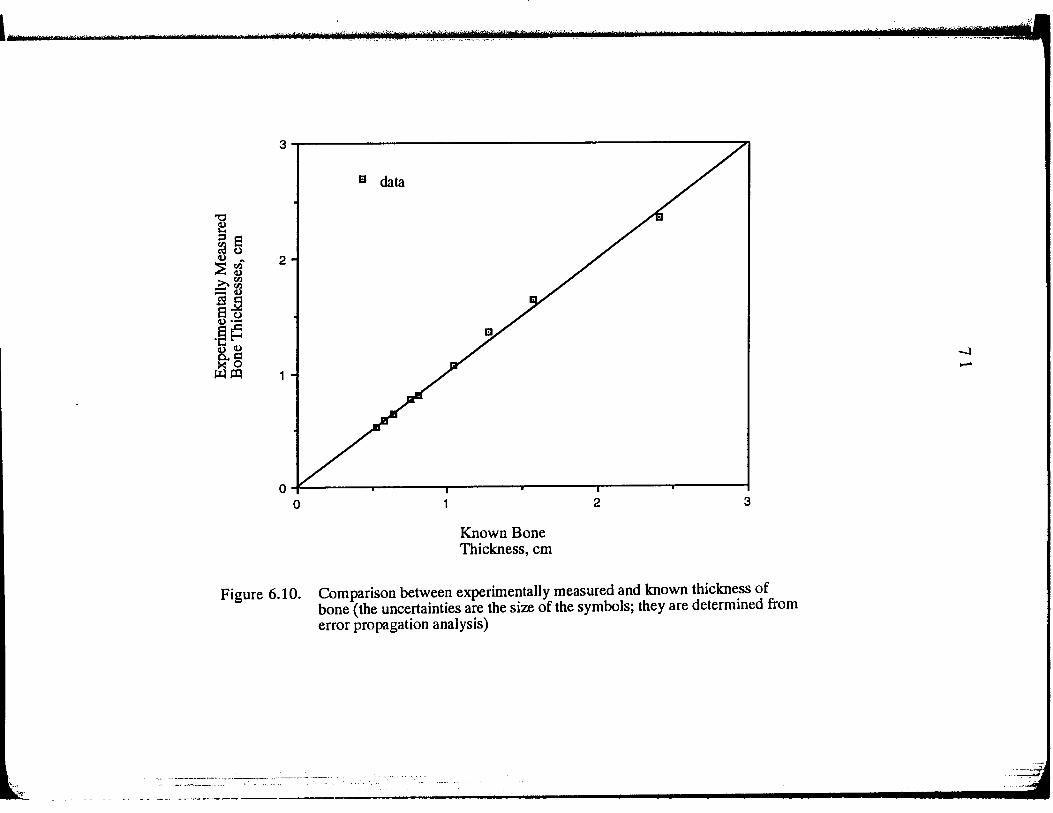
"'0 ~ ::s 8 ~ 0

~t >.1:/l _oo

- (1) ~..e 8o (1)·-

.§~ ~§ ~III

3

B data

2

1

0~------~------.-------r-------r-----~~----~ 0 1

Known Bone Thickness, em

2 3

Figure 6.10. Comparison between experimentally measured and known thickness of bone (the uncertainties are the size of the symbols; they are determined from error propagation analysis)

-.l -

----- -·-~ .. ---------------------------....--

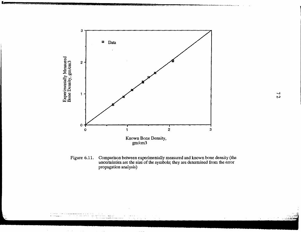
"0 0 '"'M ~8 :J.Q :a~ >.. ~ =» ,S.!:: c:l~ 00

.~Q ~§ ~~

3~------------------------------------------------~

a Data

2

1

0 1

Known Bone Density, gm/cm3

2 3

Figure 6.11. Comparison between experimentally measured and known bone density (the uncertainties are the size of the symbols; they are determined from the error propagation analysis)

-.I N

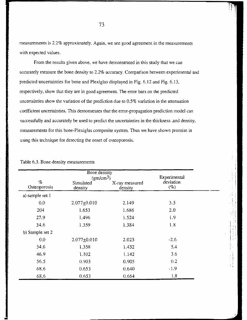
73

measurements is 2.2% approximately. Again, we see good agreement in the measurements

with expected values.

From the results given above, we have demonstrated in this study that we can

accurately measure the bone density to 2.2% accuracy. Comparison between experimental and

predicted uncertainties for bone and Plexiglas displayed in Fig. 6.12 and Fig. 6.13,

respectively, show that they are in good agreement. The error bars on the predicted

uncertainties show the variation of the prediction due to 0.5% variation in the attenuation

coefficient uncertainties. This demonstrates that the error-propagation prediction model can

successfully and accurately be used to predict the uncertainties in the thickness ,and density,

measurements for this bone-Plexiglas composite system. Thus we have shown promise in

using this technique for detecting the onset of osteoporosis.

Table 6.3. Bone density measurements

Bone density (gm/cm3) Experimental

% Simulated X-ray measured deviation Osteoporosis density density (%)

a) sample set 1

0.0 2.077±0.010 2.149 3.5

204 1.653 1.686 2.0

27.9 1.496 1.524 1.1.)

34.6 1.351.) 1.384 1.8

b) Sample set 2

0.0 2.077±0.010 2.023 -2.6

34.6 1.358 1.432 5.4

46.1.) 1.102 1.142 3.6

56.5 0.1.)03 0.905 0.2

68.6 0.653 0.640 -l.Y 68.6 0.653 0.664 1.8

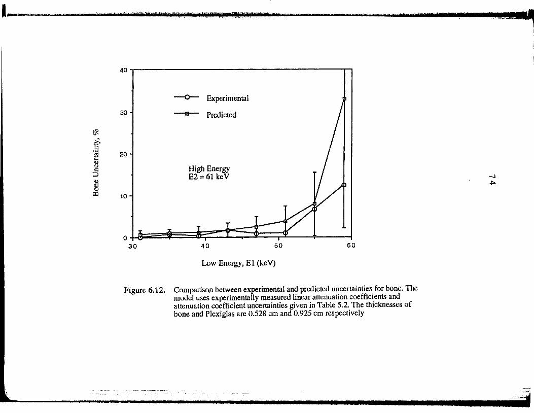
1-.llllilill~ ,,.. ..... l

~ ~ ..... r:: ·-~ ~ ;5

<U r:: 0 ~

1 5 • t .- .. 1 r ·rrmr 7 r pm

40~----------------------------------------~~

-o- Experimental

30 -- Predicted

20

High Energy E2= 61 keV

10

30 40 50 60

Low Energy, El (keV)

Figure 6.12. Comparison between experimental and predicted uncertainties for bone. The model uses experimentally measured linear attenuation coefficients and attenuation coefficient uncertainties given in Table 5.2. The thicknesses of bone and Plexiglas are 0.528 em and 0.925 em respectively

-l .j::>.

* ~ .... c:: -~

c1.) u c::

::::> til ro bn "><

c1.)

a:

ax· " tim t

60

-o- Experimental 50

El Predicted

40

30 High Energy E2=61 keV

-.l 20 lJ\

10

30 40 50 60

Low Energy, El (keV)

Figure 6.13. Comparison between experimental and predicted uncertainties for Plexiglas. The model uses experimentally measured linear attenuation coefficients and attenuation coefficient uncertainties given in Table 5.2. The thicknesses of bone and Plexiglas are 0.528 em and 0.925 em respectively

- ---""'

-- -------··-------------------------....iiliiiiiil

! l ' j i i i'

76

n.4 Aluminum-aluminum corrosion composite measurements

6.4.1 Optimization study

The prediction model for detennining the optimum energy-pair for the corrosion study

uses experimental linear attenuation coefficients and experimental attenuation coefficient

uncertainties given in Table 5.3. The beam transmission uncertainties are not present in our

predictions for reasons discussed above. The predicted uncertainty models for AI 2024 and

Al(OH)3 are shown in Fig. 6.14 and Fig. 6.15 respectively. For this corrosion study, the

optimum energy-pair is 31 keV for the low energy, E }, and 61 keV for the high energy, E2.

All subsequent experimental measurements in this section will use this energy-pair.

A similar observation is noted in this corrosion optimization study as was seen in the

bone-Plexiglas optimization study. The predicted uncertainty curves converged as the value of

E2 increased. This means that choosing energies that are farther apart than those energies used

in this model will not significantly improve the thickness, or density, measurements.

6.4.2 Aluminum-aluminum corrosion composite results and discussions

The results from this study are shown in Table 6.4. The percentage of material loss of

aluminum 2024 varied from 0% to 50% in our samples. Comparison between experimentally

measured and caliper measured aluminum 2024 thicknesses are displayed in Fig. 6.16. The

predicted uncertainty for the measured aluminum 2024 in the figure is 3.1 %. There is a

systematic deviation in the aluminum 2024 results. Most of the measured aluminum 2024

thicknesses show a negative bias relative to the caliper thickness measurements. The average

aluminum 2024 experimental bias is less than 4%, in close agreement with the predicted

uncertainty of 3.1 %. Thus we have shown that this technique can measure the material loss of

aluminum 2024 with an accuracy of 4%. If this anomaly can be addressed, we predict that we

can improve the current uncertainty of 4% to about 2% in the metal thickness measurements.

n,,, .. :I :

. )

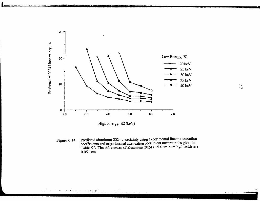
~ ~ .... c -~

8 c ::::> "<t N 0 N :( 13 ..... C)

:a ~ ~

30

20 Low Energy, E1

• 20keV 6 25keV

• 30keV

• 35keV 10 tl 40keV

0~--~--.---~--.---~--.---~--~--~~

20 30 40 50 60 70

High Energy, E2 (ke V)

Figure 6.14. Predicted aluminum 2024 uncertainty using experimental linear attenuation coefficients and experimental attenuation coefficient uncertainties given in Table 5.3. The thicknesses of aluminum 2024 and aluminum hydroxide are 0.051 em

-.l -.l

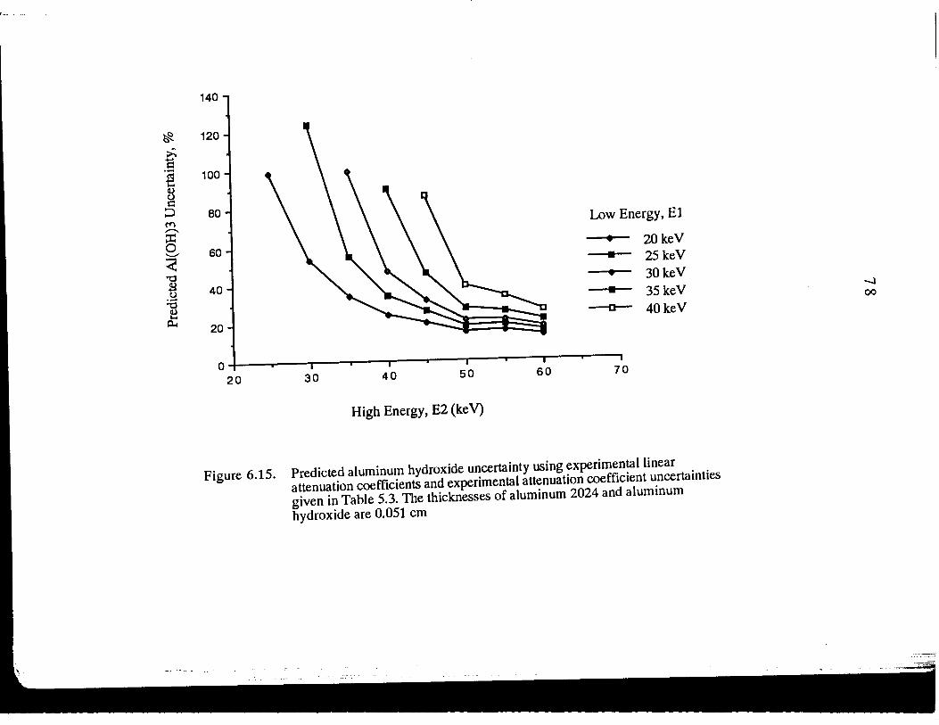
~ ;;. ..... c:: -~

B c:: ::::> ('f) ,........ :I:: 0 '-"

< "t:J ~ (.)

;a ~

p..,

140

120

100

80 Low Energy, E1

20keV 60 • 25keV

• 30keV 40 • 35keV

D 40keV

20

0 20 30 40 50 60 70

High Energy, E2 (ke V)

Figure 6.15. Predicted aluminum hydroxide uncertainty using experimental linear attenuation coefficients and experimental attenuation coefficient uncertainties given in Table 5.3. The thicknesses of aluminum 2024 and aluminum hydroxide are 0.051 em

-.l 00

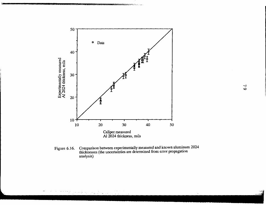
so.----------------------------------0 Data

40

"BCI) ..,._ ::s·-Cl)e ~ ~ e~

II.)

30 £J2 5.~ Q.t:: 11.) ....

e-v ·c:: M

~~ r.x:~< 20

10~--~---r--~----r---~--~--~--~

10 20 40 50

Caliper measured AI 2024 thickness, mils

Figure 6.16. Comparison between experimentally measured and known aluminum 2024 thicknesses (the uncertainties are detennined from error propagation analysis)

-...l

\0

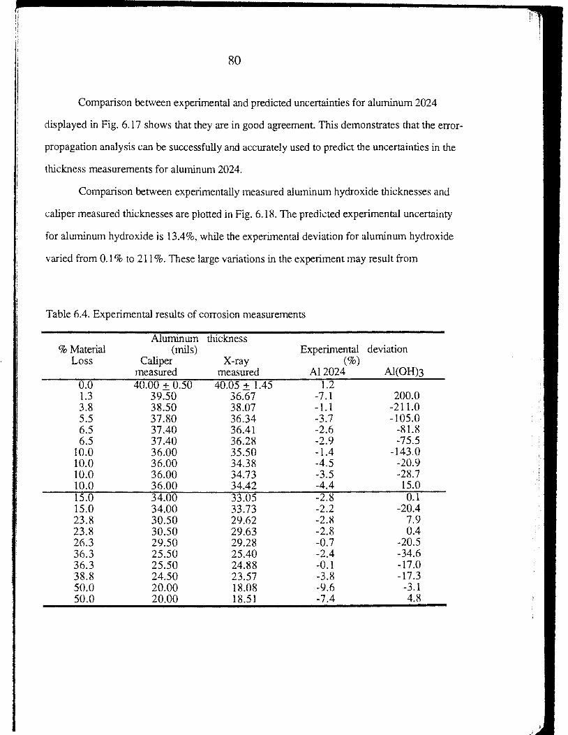
RO

Comparison between experimental and predicted uncenainties for aluminum 2024

displayed in Fig. 6.17 shows that they are in good agreement. This demonstrates that the error­

propagation analysis can be successfully and accurately used to predict the uncertainties in the

thickness measurements for aluminum 2024.

Comparison between experimentally measured aluminum hydroxide thicknesses and

caliper measured thicknesses are plotted in Fig. 6.lfl. The predicted experimental uncertainty

for almninum hydroxide is 13.4%, while the experimental deviation for aluminum hydroxide

varied from 0.1% to 211%. These large variations in the experiment may result from

Table 6.4. Experimental results of corrosion measurements

Aluminum thickness %Material (mils) Experimental deviation

Loss Caliper X-ray (%) measured measured Al2024 Al(OH)3

0.0 40.00 ± 0.50 40.05 ± 1.45 1.2 1.3 39.50 36.67 -7.1 200.0 3.8 38.50 38.07 -1.1 -211.0 5.5 37.80 36.34 -3.7 -105.0 6.5 37.40 36.41 -2.6 -81.8 6.5 37.40 36.28 -2.9 -75.5

10.0 36.00 35.50 -1.4 -143.0 10.0 36.00 34.38 -4.5 -20.9 10.0 36.00 34.73 -3.5 -28.7 10.0 36.00 34.42 -4.4 15.0 15.0 34.00 33.05 -2Js 0.1 15.0 34.00 33.73 -2.2 -20.4 23.8 30.50 29.62 -2.8 7.9 23.8 30.50 29.63 -2.8 0.4 26.3 29.50 29.28 -0.7 -20.5 36.3 25.50 25.40 -2.4 -34.6 36.3 25.50 24.88 -0.1 -17.0 38.8 24.50 23.57 -3.8 -17.3 50.0 20.00 18.08 -9.6 -3.1 50.0 20.00 18.51 -7.4 4.8

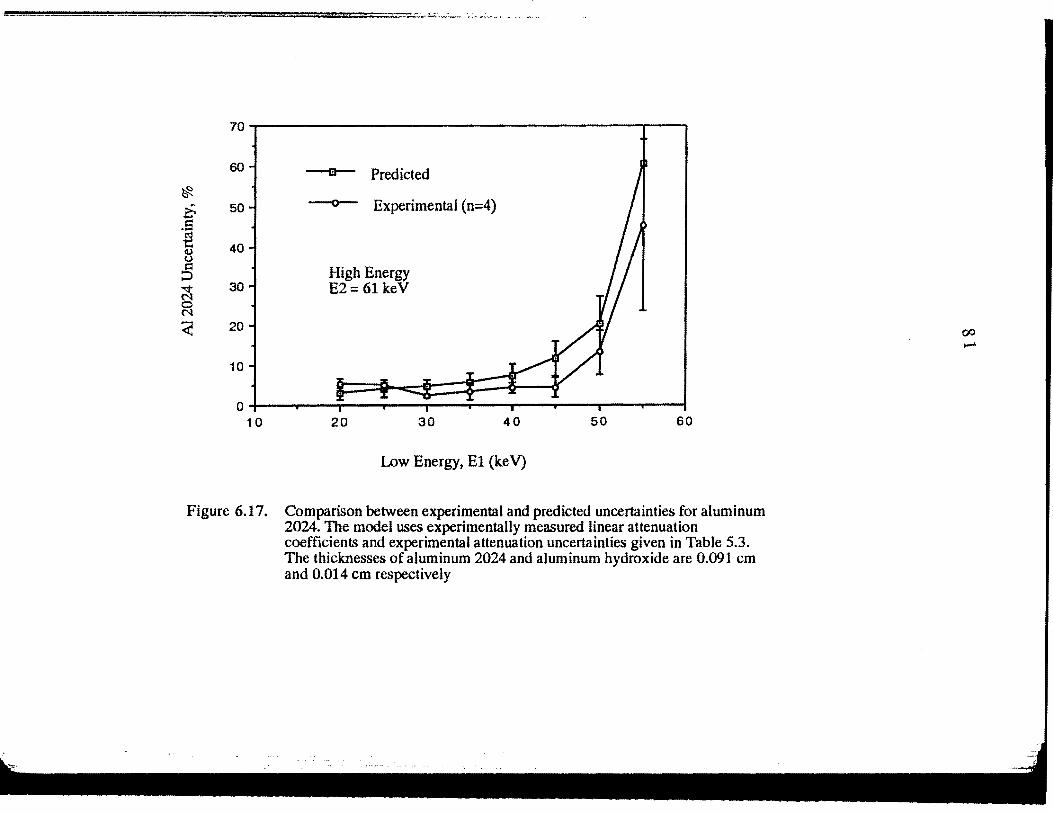
70

60

~

~ 50 t:l

·~ 40 tU

0 t:l

:::::> -.::1" 30 N 0 N

< 20

10

0 10

-a-- Predicted

--o- Experimental (n=4)

High Energy E2= 61 keY

20 30 40

Low Energy, El (keY)

50 60

Figure 6.17. Comparison between experimental and predicted uncertainties for aluminum 2024. The model uses experimentally measured linear attenuation coefficients and experimental attenuation uncertainties given in Table 5.3. The thicknesses of aluminum 2024 and aluminum hydroxide are 0.091 em and 0.014 em respectively

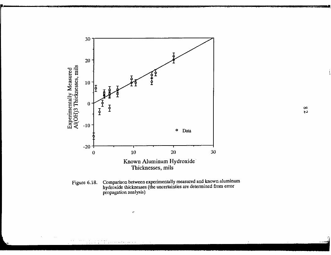
30~----------------------------------

20

0 Data

-207-----------~-----------r-----------------------T----------~----------~

0 10 20

Known Aluminum Hydroxide· Thicknesses, mils

30

Figure 6.18. Comparison between experimentally measured and known aluminum hydroxide thicknesses (the uncertainties are determined from error propagation analysis)

,.

R3

inconsistent packing of the aluminum hydroxide powder in the corrosion samples. This

assumption is confirmed by Fig. 6.19, showing a comparison between experimental and

predicted uncertainties for aluminum hydroxide. Here, we have a sample with a packed density

for aluminum hydroxide that is different than the packed density for aluminum hydroxide used

to measure the linear attenuation coefficient Although we see a shift in the experimental

uncertainties due to the density variation, the experimental uncertainty curve behaved as

expected; i.e., the uncertainty decreases as the energy-pair moved further away from one

another. In addition, the error bars on the predicted uncertainties show the variation of the

prediction due to 0.5% variation in the linear attenuation coefficient uncertainties. This means

that the difference in the thickness measurements cannot be accounted for by the linear

attenuation uncertainty; instead. the difference is a result of the variations in the packed density

for aluminum hydroxide.

The line drawn across the results in Table 6.4 indicates the FAA safety tolerance

concerning material loss due to corrosion. Below this line are aluminwn samples with

unacceptable material loss of more than 10%. By observation, we see that this energy­

dispersive technique gives uniform accuracy in the thickness measurements for AI 2024 for

thicknesses ranging from 20 mils to 40 mils. Therefore we have successfully demonstrated that

this x-ray technique can quantitatively measure the thickness of alwninum 2024 metal and

detect the presence of its corrosion product - aluminum hydroxide.

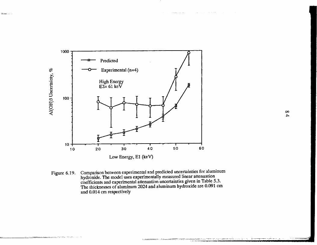
1000~--------------------------------------~-----

100

-a-- Predicted

-o- Experimental (n=4)

High Energy E2= 61 keV

10;---~----r---~--~----T---~----~--~--~--~ 10 20 30 40 50 60

Low Energy, El (keV)

Figure 6.19. Comparison between experimental and predicted uncertainties for aluminum hydroxide. The model uses experimentally measured linear attenuation coefficients and experimental attenuation uncertainties given in Table 5.3. The thicknesses of aluminum 2024 and aluminum hydroxide are 0.091 em and 0.014 em respectively

R5

7. CONCLUSIONS

This thesis has been an experimental study of an energy-dispersive x-ray NDE

technique for the purpose of material characterization of composite systems. Such information

can be used to quantitatively detennine material variation of each of the components in the

composite which in tum can be used for estimating the material properties such as the strength

of the composite and the densities of its components.

This study demonstrated the principle of the x-ray energy-dispersive technique for

quantitative material characterization in composite systems. This x-ray technique worked well

for detennining the thicknesses and densities for composite components having the higher

linear attenuation coefficient For example, this technique accurately determined material

thickness of epoxy-resin and aluminum-metal. and the density of bone, to 4% or less in each of

the corresponding composite-systems. Looking at Eq. 7 we see that the product of the

attenuation coefficient and the thickness enters the formulae. For an element that has a relatively

large attenuation coefficient, a small change in the thickness will have the same effect on the

result as a large change in the thickness of an element that has a relatively small attenuation

coefficient Therefore, the thickness measurements for the elements with lower linear

attenuation coefficients were less accurate, in their respective composite systems.

The accuracy of this energy-dispersive technique is dictated by the uncertainties in the

linear attenuation coefficient measurements. For the attenuation coefficients of solids. the

uncertainty comes from the uncertainty of the caliper measurement; while for the powder. such

as aluminum hydroxide, the uncertainty comes from the caliper measurement, and moreover

from the powder-packed density in the vial. Therefore care must be taken in making caliper

measurements for linear attenuation coefficient calculations.

86

The use of the germanium detector and multichannel analyzer provided high energy

sensitivity, but certain obvious limitations are present, such as the inspection time. The

inspection time for the current system is about a day for point-measurement This fails to meet

the demand for a rapid in-service NDE inspection technique. In addition, the experimental

setup itself is a limitation, because this technique requires access to two opposite sides of the

sample. And frequently, access to two sides is limited or impossible due to intervening

structures. Although this x-ray technique presented in this study requires access to both sides

of the composite samples, this study nevertheless gives us confidence to develop an x-ray

backscatter technique that will require access to only one side of the sample. This will make in­

service material characterization more practical.

The limitation for the immediate development of a rapid in-service inspection tool,

using this x-ray technique, is the amplifier and the MCA systems. The amplifier and the MCA

systems are the weakest link in the electronic system's throughput capabilities. The amplifier

has a pulse-shaping dead-time of about 5- 80 j.lsec per pulse depending on the count rate. The

MCA can have dead-time greater than 30% when count rate exceeds 30 kHz.

The need for the long inspection time is due to the need to acquire high counting

statistics. The future of the research in this technique will be to replace the MCA with a single­

channel analyzer (SCA); this will significantly improve the inspection time. In a two­

component composite, we only need two energies to characterize the composite. Thus we only

need two SCA to monitor the two energies. The energy sensitive response of the germanium

detector can be gated using a SCA. By selecting an upper and lower voltage window, we can

regulate the energy of x-ray photons monitored. The advantage that the SCA has over MCA is

its high count rate. SCA can handle count rate upto 400kHz. Thus it is possible to reduce the

current inspection time by 50 times, approximately. From this, we can reduce the inspection

time from 24 hours to half-an-hour. There is a drawback in using this SCA setup; the current

87

SCA system cannot perform the PUR subtraction on the signals. Though this can be overcome

by constructing an electronic device that monitors the incoming signal for Pile-Up-Rejection.

Therefore in this thesis we have demonstrated this new x-ray energy-dispersive NDE

technique is capable of characterizing material compositions in different composite systems

with two components. We have also demonstrated that the error-propagation analysis can be

used to predict the experimental thickness uncertainty. We have demonstrated with

experimental results that error-propagation analysis can accurately predict the optimum energy

pair and experimental uncertainty. Thus the analysis can be used as a preliminary study to

evaluate the accuracy attainable with this technique before any experiment is performed.

88

REFERENCES

1. A Practical Guide to High Count Rate Gennanium gamma Spectroscopy. Application

note form Canberra Nuclear Products Group, Meriden, CT; ca. 1992.

2. H.L. Atkins, W. Hausser and H. Kraner, "Absorption Edge Transmission Scanning"

American Journal of Roentgen 114 (1972); 176-180.

3. M.J. Berger and J.H. Hubbell. "XCOM: Photon Cross-Sections on a Personal

Computer." NlST Resport #NBSIR 87-3597 (1987).

4. P.R. Bevington. Data Reduction and Error Analysis for the Physical Sciences.

New York; McGraw-Hill (1969).

5. J.R. Cameron and J. Sorenson. "Measurement of Bone Mineral in vivo: An Improved

Method." Science 142 ( 1963 ); 230-232.

6. R. Deslattes. "Estimates of x-ray attenuation coefficients for the elements and their

compounds." Acta. Cryst. A25 ( 1969); 89-93.

7. L. Gerward. "X-ray attenuation coefficients of carbons in energy range of 5 to 20 keY."

Acta Cryst. A39 (1983); 322-325.

8. B.R. Kerur, S.R. Thontadarya and B. Hanumaiah. "X-ray Attenuation Coefficients at

6.46 keY and the Validity of the Mixture Rule for Compounds." X-ray Spectrometry

22 (1993); 13-16.

9. G.F. Knoll. Radiation Detection and Measurement. New York; John Wiley and sons

(1979).

10. K. Kouris, and N.M. Spyrou and D.F. Jackson. "Minimum Detectable quantities of

elements and compounds in a biological matrix." Nuclear Instruments and Methods

187 (1981 ); 539-545.

R9

11. K. Kouris and N .M. Spyrou. "Usefulness of photon mass attenuation coefficients in

elemental analysis." Nuclear Instruments and Methods ill (1978); 477-483.

12. H.W. Kraner, J.L. Alberi and H.L. Atkins. "Transmission Scanning Using a

Continuous X-ray Source." IEEE trans. Nucl. Sci. 20 (1972); 389-401.

13. S.M. Lee. International Encyclopedia of Composites. New York; VCH Publishers

Inc.( 1990).

14. R.W. Leonard. "Airframe and Aerodynamic." Aeronautics and Astronautics Vol. 14,

No.2. (1976); 18-31.

15. Mark's Standard Handbook for mechanical Engineering. Ninth Edition; New York;

MacGraw-Hill (1978).

16. B.G. Martin. II An Analysis of Radiographic Techniques for Measuring Resin Content

in Graphite Fiber Reinforced Resin Composites. II Material Evaluation 35

( 1977); 65-68.

17. R.B. Mazess, W.W. Peppler, C.H. Chesnut III, W.B. Nelp, S.H. Cohnand I. Zanzi.

"Total Body Bone Mineral and Lean Body Mass by Dual-Photon Absorptiometry: II.

Comparison with Total Body Calciun by Neutron Activation Analysis." Calcified

Tissue International J3_ (1981 ); 361-363.

18. R.B. Mazess, W.W. Peppler, J.E. Harison and K.G. McNeill. "Total Body Bone

Mineral and Lean Body Mass by Dual-Photon Absorptiometry: III. Comparison

with Trunk Calcium by Neutron Activation Analysis." Calified Tissue International

n c 1981 ); 365-368.

19. W.H. McMaster, N.Kerr Del Grande, J.H.Mallet, J.H.Hubbell. "Compilation of X-ray

Cross Sections." National Bureau of Standard UCRL-50174 Sec.II Rev. I. (1971).

90

20. NASA Reference Publication 1092, "Standard Tests for Toughened Resin Composite."

rev. ed. (July 1983).

21. W.W. Peppler and R.B. Mazess. "Total Body Bone Mineral and Lean Body Mass by

Dual-Photon Absorptiometry: I. Theory and Measurement Procedure." Calcified

Tissue International 33 (1981 ); 353-359.

22. F.P. Povinelli, J.M.Klineberg and J.J Kraner. "Improving Aircraft Energy

Efficiency." Aeronautics and Astronautics Vol. .1.6., No. 7.8 (1978); 38-46.

23. S.J. Reiderer and C.A. Mistretta. " Selective Iodine Imaging Using K-edge Energies in

Computerized X-ray Tomography." Medical Physics~ (1977); 474-481.

24. M.E. Rose and M.M. Shapiro. "Statistical error and absorption experiments." Physical

Review Vol. 74, No . .12.; (1948); 1853-1864.

25. I. Rudich, L. Lesensky and F. Kapelewski. "High-X-Ray Flux: High Contrast

Radiography of Carbon Fiber-Reinforced Epoxy Aircraft Stuctures." Materials

Evaluation 44 ( 1986); 1158-1184.

26. Shull, B.E. "Nondestructive X-ray methods for characterization of advanced aerospace

materials." MS Thesis; Iowa State University, Ames, lA; (1989).

27. J. Ting, T. Jensen and J.N. Gray. "Quantitative determination of material composition

using energy sensitive measurements." In Review of Progress in Quantitative

Nondestructive Evaluation; Vol.llB; Eds. D.O. Thompson and D.E. Chimenti.

New York; Plenum Press; (1991 ); 1499-1505.

28. J. Ting, T. Jensen and J.N. Gray. "Using energy dispersive x-ray measurements for

quantitatively determination of material loss due to corrosion." In Review of

Progress in Quantitative Nondestructive Evaluation; Vol.12B; Eds. D.O. Thompson

and D.E. Chimenti. New York; Plenum Press; (1992); 1963-1969.

91

29. L.F. Volsteen. "Composite Aircraft Structures." In Fiberous Composites in Structural

Design. Eds. E.M. Lenoe, D.W. Oplinger, and J.J. Burke. New York; Plenum

Press; (1980); 7-24.

30. D.E. Watt. "Optimum photon energies for the measurement of bone and fat fractions."

British Journal of Radiography 4g (1975); 265-274.