probabilistic seismic hazard analysis: a sensitivity … · olasılıksal sismik tehlike analizinin...
TRANSCRIPT

PROBABILISTIC SEISMIC HAZARD ANALYSIS: A SENSITIVITY STUDY WITH RESPECT TO DIFFERENT MODELS
A THESIS SUBMITTED TO THE GRADUATE SCHOOL OF NATURAL AND APPLIED SCIENCES
OF MIDDLE EAST TECHNICAL UNIVERSITY
BY
NAZAN YILMAZ ÖZTÜRK
IN PARTIAL FULFILLMENT OF THE REQUIREMENTS FOR
THE DEGREE OF DOCTOR OF PHILOSOPHY IN
CIVIL ENGINEERING
FEBRUARY 2008

Approval of the thesis:
PROBABILISTIC SEISMIC HAZARD ANALYSIS: A SENSITIVITY STUDY WITH RESPECT TO DIFFERENT MODELS
submitted by NAZAN YILMAZ ÖZTÜRK in partial fulfillment of the requirements for the degree of Doctor of Philosophy in Civil Engineering Department, Middle East Technical University by, Prof. Dr. Canan Özgen _____________________ Dean, Graduate School of Natural and Applied Sciences
Prof. Dr. Güney Özcebe _____________________ Head of Department, Civil Engineering
Prof. Dr. M. Semih Yücemen _____________________ Supervisor, Civil Engineering Dept., METU Examining Committee Members: Prof. Dr. Ali Koçyiğit _____________________ Geological Engineering Dept., METU
Prof. Dr. M. Semih Yücemen _____________________ Civil Engineering Dept., METU
Prof. Dr. Reşat Ulusay _____________________ Geological Engineering Dept., Hacettepe University
Assoc. Prof. Dr. Ahmet Yakut _____________________ Civil Engineering Dept., METU
Assoc. Prof. H. Şebnem Düzgün _____________________ Mining Engineering Dept., METU Date: 08.02.2008

iii
I hereby declare that all information in this document has been obtained and presented in accordance with academic rules and ethical conduct. I also declare that, as required by these rules and conduct, I have fully cited and referenced all material and results that are not original to this work.
Name, Last name : Nazan Yılmaz Öztürk
Signature :

iv
ABSTRACT
PROBABILISTIC SEISMIC HAZARD ANALYSIS: A SENSITIVITY STUDY WITH RESPECT TO DIFFERENT MODELS
Yılmaz Öztürk, Nazan
Ph.D., Department of Civil Engineering
Supervisor: Prof. Dr. M. Semih Yücemen
February 2008, 253 pages
Due to the randomness inherent in the occurrence of earthquakes with respect to
time, space and magnitude as well as other various sources of uncertainties, seismic
hazard assessment should be carried out in a probabilistic manner.
Basic steps of probabilistic seismic hazard analysis are the delineation of seismic
sources, assessment of the earthquake occurrence characteristics for each seismic
source, selection of the appropriate ground motion attenuation relationship and
identification of the site characteristics. Seismic sources can be modeled as area and
line sources. Also, the seismic activity that can not be related with any major
seismic sources can be treated as background source in which the seismicity is
assumed to be uniform or spatially smoothed. Exponentially distributed magnitude
and characteristic earthquake models are often used to describe the magnitude
recurrence relationship. Poisson and renewal models are used to model the
occurrence of earthquakes in the time domain.

v
In this study, the sensitivity of seismic hazard results to the models associated with
the different assumptions mentioned above is investigated. The effects of different
sources of uncertainties involved in probabilistic seismic hazard analysis
methodology to the results are investigated for a number of sites with different
distances to a single fault. Two case studies are carried out to examine the influence
of different assumptions on the final results based on real data as well as to illustrate
the implementation of probabilistic seismic hazard analysis methodology for a large
region (e.g. a country) and a smaller region (e.g. a province).
Keywords: Seismic Hazard, Seismic Source, Magnitude Distribution, Renewal,
Poisson, Earthquake.

vi
ÖZ
OLASILIKSAL SİSMİK TEHLİKE ANALİZİ: DEĞİŞİK MODELLERE GÖRE DUYARLILIK ÇALIŞMASI
Yılmaz Öztürk, Nazan
Doktora, İnşaat Mühendisliği Bölümü
Tez Yöneticisi: Prof. Dr. M. Semih Yücemen
Şubat 2008, 253 sayfa
Deprem oluşumlarının zaman, yer ve büyüklük bakımından gösterdikleri rassallık
ve diğer çeşitli belirsizlikler nedeniyle sismik tehlikenin belirlenmesi olasılığa
dayanan yöntemlerle yapılmalıdır.
Olasılıksal sismik tehlike analizinin başlıca adımları sismik kaynakların ve bu
kaynakların her biri için deprem oluşum özelliklerinin belirlenmesi, uygun azalım
ilişkisinin seçilmesi ve sahadaki zemin özelliklerinin saptanmasıdır. Sismik
kaynaklar alan ve çizgi kaynaklar olarak modellenebilir. Ayrıca, herhangi bir ana
sismik kaynak ile ilişkilendirilemeyen sismik etkinlik, depremselliğin bir biçimli ya
da mekansal olarak yaygınlaştırılmış olduğu kabul edilen arka plan kaynak olarak
incelenebilir. Üstel dağılımlı büyüklük ve karakteristik deprem modelleri büyüklük-
tekrarlanma ilişkilerini tanımlamak için en sık kullanılanlardır. Poisson ve
yinelenme modelleri depremlerin zaman uzayındaki oluşumlarını modellemek için
kullanılmaktadır.

vii
Bu çalışmada sismik tehlike sonuçlarının yukarıda bahsedilen değişik varsayımlarla
ilişkilendirilen modellere duyarlılığı araştırılmıştır. Olasılıksal sismik tehlike
analizindeki değişik belirsizliklerin sonuçlara etkileri bir faydan oluşan sismik
kaynağa değişik uzaklıklarda yer alan birkaç saha için araştırılmıştır. Değişik
varsayımların nihai sonuçlara olan etkisini gerçek veriye dayalı olarak incelemek ve
olasılıksal sismik tehlike yönteminin büyük (bir ülke gibi) ve daha küçük bir
bölgenin (bir kent gibi) sismik tehlikesinin belirlenmesi için uygulanmasını
göstermek amacıyla iki örnek çalışma yapılmıştır.
Anahtar Kelimeler: Sismik Tehlike, Sismik Kaynak, Büyüklük Dağılımı,
Yinelenme, Poisson, Deprem.

viii
to my family…

ix
ACKNOWLEDGEMENTS
This study was accomplished under the supervision of Prof. Dr. M. Semih
Yücemen. I would like to thank him for his continuous guidance, advice, patience,
and support throughout the period of this study. His supervision made my biggest
academic achievement possible. I am grateful to him for making my way to the
academic world.
I want to thank Assoc. Prof. Dr. Ahmet Yakut and Assoc. Prof. Dr. H. Şebnem
Düzgün for their valuable suggestions and encouraging comments during the
progress of this dissertation.
I would like to thank Prof. Dr. Ali Koçyiğit from the Geological Engineering
Department, for his contributions towards my understanding of tectonics and in
particular, sharing his knowledge on the faults located in Turkey with me.
I want to thank Prof. Dr. Reşat Ulusay for his detailed review of the manuscript of
this dissertation and his valuable suggestions.
This thesis started in the structural mechanics laboratory of Civil Engineering
Department. I would like to thank all my friends from the lab for their help and
support.
The majority of this study is carried at the Earthquake Engineering Research Center
(EERC) at METU. I want to thank to Prof. Dr. M. Semih Yücemen once again for
providing the office there and Asst. Prof. Dr. Altuğ Erberik and İlker Kazaz for
their supports during all stages of this dissertation.
Special thanks go to my lifelong friend (or my little sister) Dr. Ayşegül Askan-
Gündoğan for being nearby in the beginning of this study as well as catching up in

x
the end. In the mean time, via long-distance phone calls, she proved me that
distances do not matter in friendships.
I would like to thank Dr. Erol Kalkan for devoting his time and sharing the
documents on the subject of this study and the code for spatially smoothed
seismicity model.
My good friends; Eser Tosun, Selim Günay, Berna Unutmaz, Emriye Kazaz,
Sermin Oğuz Topkaya, Sergen Bayram and Altuğ Bayram, deserve thanks for their
support and patience.
I also would like to extend my thanks to the staff of the Earthquake Research
Department at the General Directorate of Disaster Affairs, especially Dr. Murat
Nurlu, current director of the Laboratory Division, for his support and
understandings. I owe thanks to Cenk Erkmen, Hakan Albayrak, Tülay Uran,
Tuğbay Kılıç and Ulubey Çeken for their theoretical and technical supports.
I would like to thank my father, mother, sister and brother for their love,
understanding and encouragement throughout my life and for forgiving me for all
the postponed get-togethers with them. I promise to make up for those times after I
finish.
Finally, I would like to give my thanks to my husband for his invaluable support
during this long period.

xi
TABLE OF CONTENTS
ABSTRACT………………………………………………………………………... iv
ÖZ………………………………………………………………………………….. vi
ACKNOWLEDGEMENTS………………………………………………………...ix
TABLE OF CONTENTS…………………………………………………………...xi
LIST OF TABLES………………………………………………………………....xv
LIST OF FIGURES………………………………………………………………xvii
CHAPTER
1. INTRODUCTION…………………………………………………………..1
1.1 GENERAL……………………………………………………………...1
1.2 LITERATURE SURVEY………………………………………………2
1.3 OBJECTIVES AND SCOPE OF THE STUDY………………………. 6
2. ALTERNATIVE MODELS APPLIED IN SEISMIC HAZARD
ANALYSIS………………………………………………………………….8
2.1 INTRODUCTION……………………………………………………... 8
2.2 DETERMINISTIC SEISMIC HAZARD ANALYSIS………………... 9
2.3 PROBABILISTIC SEISMIC HAZARD ANALYSIS……………….. 13
2.3.1 Seismic Sources………………………………………………... 14
2.3.2 Magnitude Recurrence Relationship…………………………... 20
2.3.3 Modeling of Earthquake Occurrences…………………………. 25
2.3.4 Attenuation Relationships (Ground Motion Prediction
Equations)……………………………………………………... 30
2.3.4.1 Attenuation Models Developed for Other Countries…. 31
2.3.4.1.1 Abrahamson and Silva (1997)……………... 31
2.3.4.1.2 Boore et al. (1997)…………………………. 34
2.3.4.1.3 Sadigh et al. (1997)………………………… 36
2.3.4.1.4 Ambraseys et al. (1996)……………………. 41

xii
2.3.4.2 Attenuation Models Developed for Turkey…………... 43
2.3.4.2.1 İnan et al. (1996)……………………………43
2.3.4.2.2 Aydan et al. (1996) and Aydan (2001)……... 43
2.3.4.2.3 Gülkan and Kalkan (2002), Kalkan
and Gülkan (2004)………………………….44
2.3.4.2.4 Özbey et al. (2004)…………………………. 47
2.3.4.2.5 Ulusay et al. (2004)…………………………48
2.3.5 Seismic Hazard Calculations…………………………………... 50
2.3.6 Consideration of Uncertainties………………………………… 51
2.3.6.1 Uncertainty Due to Attenuation Equation…………….. 52
2.3.6.2 Uncertainty in the Spatial Distribution of Earthquakes..60
2.3.6.3 Uncertainty in the Magnitude Distribution…………… 77
2.3.6.4 Uncertainty in the Temporal Distribution of
Earthquakes…………………………………………… 80
2.3.6.5 Uncertainties in Earthquake Catalogs…………………. 87
2.3.7 Logic Tree Methodology………………………………………. 87
2.3.8 Deaggregation of Seismic Hazard……………………………... 90
3. CASE STUDY FOR A COUNTRY: SEISMIC HAZARD MAPPING
FOR JORDAN…………………………………………………………….. 93
3.1 INTRODUCTION……………………………………………………. 93
3.2 PREVIOUS PROBABILISTIC SEISMIC HAZARD ASSESSMENT
STUDIES FOR JORDAN……………………………………………..94
3.3 ASSESSMENT OF SEISMIC HAZARD FOR JORDAN…………… 96
3.3.1 Seismic Database and Seismic Sources………………………... 96
3.3.1.1 Seismic Database……………………………………… 96
3.3.1.2 Seismic Sources……………………………………….. 99
3.3.2 Alternative Models……………………………………………. 103
3.3.2.1 Model 1………………………………………………. 103
3.3.2.2 Model 2 and Model 3………………………………....104
3.3.2.3 Model 4………………………………………………. 105
3.3.3 Seismic Hazard Computations………………………………... 110
xiii
3.3.4 “Best Estimate” Seismic Hazard Maps for Jordan……………. 135
4. CASE STUDY FOR A REGION: SEISMIC HAZARD MAPPING FOR
THE BURSA PROVINCE………………………………………………. 145
4.1 INTRODUCTION……………………………………………………145
4.2 PREVIOUS PROBABILISTIC SEISMIC HAZARD ASSESSMENT
STUDIES FOR BURSA…………………………………………….. 146
4.3 ASSESSMENT OF SEISMIC HAZARD FOR BURSA…………….147
4.3.1 Seismic Database and Seismic Sources………………………. 147
4.3.1.1 Seismic Database…………………………………….. 147
4.3.1.2 Seismic Sources……………………………………… 150
4.3.2 Methodology………………………………………………….. 151
4.3.2.1 Seismic Hazard Resulting From Background Seismic
Activity………………………………………………. 154
4.3.2.2 Seismic Hazard Resulting From Faults……………… 173
4.3.3 “Best Estimate” of Seismic Hazard for the Bursa Province….. 187
5. SUMMARY AND CONCLUSIONS……………………………………. 196
5.1 SUMMARY…………………………………………………………. 196
5.2 DISCUSSION OF RESULTS AND MAIN CONCLUSIONS……... 197
5.3 RECOMMENDATIONS FOR FUTURE STUDIES……………….. 202
REFERENCES……………………………………………………………………205
APPENDICES
A. GRAPHS SHOWING THE DIFFERENCE BETWEEN THE SEISMIC
HAZARD RESULTS OBTAINED BY IGNORING AND
CONSIDERING RUPTURE LENGTH UNCERTAINTY……………... 217
B. EARTHQUAKE CATALOG PREPARED FOR JORDAN……………. 225
C. SEISMIC HAZARD MAPS FOR JORDAN BASED ON
DIFFERENT MODELS…………………………………………………. 230
D. MAIN SEISMIC DATABASE COMPILED FOR BURSA FROM THE
CATALOGS OF EARTHQUAKE RESEARCH DEPARTMENT,
GENERAL DIRECTORATE OF DISASTER AFFAIRS………………. 237

xiv
E. MAIN SHOCK SEISMIC DATABASE COMPILED FOR BURSA
FROM THE CATALOGS OF EARTHQUAKE RESEARCH
DEPARTMENT, GENERAL DIRECTORATE OF DISASTER
AFFAIRS………………………………………………………………... 246
CURRICULUM VITAE ………………………………………………………… 251

xv
LIST OF TABLES
TABLES
Table 2.1 Parameters of the Fault and the Scenario Earthquake Model Used
for İstanbul in This Study (JICA, 2002)……………………………... 11
Table 2.2 Mean and Median PGA Values Estimated at the Site by Using
Different Attenuation Relationships for Rock Site Condition in
DSHA…………………………………………………………………12
Table 2.3 Coefficients for the Average Horizontal Component
(Abrahamson and Silva, 1997)………………………………………. 35
Table 2.4 Smoothed Coefficients for Pseudo-Acceleration Response
Spectra (g) (Boore et al., 1997)……………………………………….37
Table 2.5 Coefficients for Rock Sites with Mw ≤ 6.5 (Sadigh et al., 1997)……. 39
Table 2.6 Coefficients for Rock Sites with Mw > 6.5 (Sadigh et al., 1997)……. 39
Table 2.7 Dispersion Relationships for Horizontal Rock Motion (Sadigh et al.,
1997)…………………………………………………………………. 40
Table 2.8 Coefficients for Deep Soil Sites (Sadigh et al., 1997)……………….. 40
Table 2.9 Coefficients of the Attenuation Relationship Proposed by
Ambraseys et al. (1996)……………………………………………… 42
Table 2.10 Coefficients of Attenuation Relationships Developed by Gülkan and
Kalkan (2002)………………………………………………………... 45
Table 2.11 Coefficients of Attenuation Relationships Developed by Kalkan and
Gülkan (2004)………………………………………………………... 46
Table 2.12 Site Class Definitions Used by Özbey et al. (2004)…………………..48
Table 2.13 Attenuation Coefficients in the Equation Proposed by
Özbey et al. (2004)…………………………………………………....49
Table 2.14 Examples of Uncertainties in Seismic Hazard Analysis
(McGuire, 2004)……………………………………………………....52

xvi
Table 2.15 Relationships between Magnitude and Rupture Length………………61
Table 2.16 Parameters of the Darıca, Adalar, Yeşilköy and Kumburgaz
Segments……………………………………………………………....68
Table 2.17 Calculations of Multi-Segment and Individual Segment
Probabilities According to the Cascade Methodology Defined by
Cramer et al. (2000)…………………………………………………...71
Table 3.1 Space and Time Windows to Identify Secondary Events
(After Deniz and Yücemen, 2005)…………………………………… 98
Table 3.2 Parameters of Seismic Sources Considered in Model 1……………..104
Table 3.3 Parameters of Seismic Sources Considered in Model 2 and
Model 3………………………………………………………………105
Table 3.4 Parameters of Seismic Sources Considered in Model 4……………..108
Table 3.5 PGA and SA (0.2 sec and 1.0 sec) Values Corresponding to
Different Return Periods for the Four Sites According to
Different Assumptions (in g)………………………………………...123
Table 4.1 b, β and ν Values Computed According to Alternative
Assumptions for the Background Seismic Activity………………… 154
Table 4.2 Maximum PGA Values (in g) Obtained from Background
Area Source with Uniform Seismicity……………………………… 156
Table 4.3 Parameters of the Fault Segments Used in This Study
(Koçyiğit, 2005; Yücemen et al., 2006)…………………………….. 174
Table 4.4 Subjective Probabilities Assigned to Different Assumptions………. 187
Table B.1 Main Shocks in the Earthquake Catalog Prepared for Jordan……….225
Table D.1 All Earthquakes in the Seismic Database Compiled for Bursa……... 237
Table E.1 Mainshocks in the Seismic Database Compiled for Bursa…………..246

xvii
LIST OF FIGURES
FIGURES
Figure 2.1 Schematic Description of DSHA for a Site…………………………... 10
Figure 2.2 Map Showing the Location of the Fault (F) Forming the Basis
for the Scenario Earthquake Model Used for İstanbul in
This Study (JICA, 2002)………………………………………………11
Figure 2.3 Schematic Description of the Classical PSHA Methodology………... 15
Figure 2.4 Linear, Bilinear and Parabolic Magnitude Recurrence Relationships
(Yücemen, 1982)……………………………………………………... 23
Figure 2.5 Characteristic Earthquake Model Proposed by
Youngs and Coppersmith (1985)……………………………………...24
Figure 2.6 Hazard Rate Functions for Different Inter-Event Time Distributions
(Matthews et al., 2002)……………………………………………….. 28
Figure 2.7 Median Peak Ground Acceleration (PGA) Curve Predicted for
Kocaeli, 1999 Earthquake by Using Kalkan and Gülkan (2004)
Attenuation Relationship at Rock Sites; Distribution of PGA Values
at 1 km Distance and the Recorded Data…………………………….. 53
Figure 2.8 (a) Probability Density Function of Ground Motion Parameter, Y,
for a Single Scenario, (b) Complementary Cumulative Distribution
Function Describing the Probability of Ground Motion Parameter
Exceeding the Level, Y, for a Single Scenario……………………….. 54
Figure 2.9 Probability Density Functions Corresponding to Different
Values of σln(PGA)……………………………………………………... 55
Figure 2.10 Hazard Curves Corresponding to Different Values of σln(PGA)……….. 56
Figure 2.11 Probability Density Functions of PGA Truncated at Different
Levels………………………………………………………………… 58

xviii
Figure 2.12 Hazard Curves Corresponding to Truncation of Attenuation
Residuals at Different Levels……………………………………….... 58
Figure 2.13 Hazard Curves Obtained by Using Different Attenuation
Relationships…………………………………………………………. 59
Figure 2.14 Locations of Fault and Sites Considered in the Analyses
Performed to Investigate the Effect of Rupture Length
Uncertainty on Seismic Hazard Results………………………………63
Figure 2.15 Differences in Seismic Hazard Values Obtained for Site 1c by
Using Different Values of Standard Deviation for Logarithm of
Rupture Length……………………………………………………….. 65
Figure 2.16 Variation of Rupture Length as a Function of Earthquake
Magnitude According to the Relationships Proposed by Wells
and Coppersmith (1994), Bonilla, et al. (1984) and Ambraseys
and Jackson(1998)……………………………………………………. 66
Figure 2.17 Seismic Hazard Curves Obtained for Site 1c by Using Different
Rupture Length Estimation Equations for Magnitude 5 Earthquake… 66
Figure 2.18 Locations of Darıca (D), Adalar (A), Yeşilköy (Y) and
Kumburgaz (K) Segments (Yücemen et al., 2006)…………………... 67
Figure 2.19 Seismic Hazard Curves Obtained by Considering Segmentation
Concept and Fault-Rupture Model…………………………………… 69
Figure 2.20 Seismic Hazard Curves Obtained for the Three Sites by Using
Cascade and Fault Segmentation Models…………………………….. 72
Figure 2.21 Locations of Sites, Line (Fault) Source and Area Source
Representing the Fault………………………………………………... 73
Figure 2.22 Seismic Hazard Curves Obtained by Using Area and
Line (Fault) Source Models…………………………………………... 74
Figure 2.23 Probability Density Functions Corresponding to Truncated
Exponential Distribution (TED) and Characteristic Earthquake
Model (CEM) with Varying Δm values……………………………… 78

xix
Figure 2.24 Probability Density Functions Corresponding to Purely
Characteristic Earthquake Model (PCEM) and Truncated
Gaussian Distribution (TGD) for Characteristic Magnitudes and
Truncated Exponential Distribution (TED) for Smaller
Magnitudes…………………………………………………………… 79
Figure 2.25 Seismic Hazard Curves for Site 4 Corresponding to: Truncated
Exponential Distributions for 4.5<m<7.5 (TED); Characteristic
Earthquake Model (CEM) with Varying Δm values;
Purely Characteristic Earthquake Model Combined with
Exponential Distribution for Smaller Magnitudes (4.5≤m≤7.0)
(PCEM&TED); Truncated Gaussian Distribution for
Characteristic Magnitudes (7.22≤m≤7.78) Combined with
Exponential Distribution for Smaller magnitudes (4.5≤m≤7.0)
(TGD&TED)…………………………………………………………. 80
Figure 2.26 Estimated Ruptures (Thick Dashed Green Lines), Modified
Mercalli Intensity (MMI) Values (Yellow Dots), Sites of
Damage Potentially Enhanced by Soft Sediments (Red Dots),
Moment Magnitude M Needed to Satisfy the Observations for a
Given Location (Red Dashed Contours) for Large Earthquakes
Occurred between A.D. 1500 and 2000 (After Parsons, 2004)………. 82
Figure 2.27 Probability Density Functions Corresponding to the BPT and LN
Distributions Based on the Mean Inter-Event Time of
µT =54 years and α=cov=0.5…………………………………………. 83
Figure 2.28 Hazard Functions Corresponding to the BPT and LN
Distributions Based on the Mean Inter-Event Time of
µT =54 years and α=cov=0.5…………………………………………. 83
Figure 2.29 Variation of Equivalent Mean Rate of Characteristic
Earthquakes Calculated Based on Eqs. (2.20) and (2.28) for the
BPT and LN Distributions……………………………………………. 85
xx
Figure 2.30 Seismic Hazard Curves for Site 4 Corresponding to the
Combinations of Renewal Model with PCEM&TED and CEM;
Poisson Model with PCEM and CEM with Δm=1.0…………………. 86
Figure 2.31 A General Logic Tree (After Risk Engineering, 2006)………………. 89
Figure 2.32 Examples of Deaggregation Graphs Obtained from a Seismic
Hazard Analysis Carried Out by Using EZ-FRISK (Risk
Engineering, 2005)…………………………………………………… 92
Figure 3.1 Map Showing the Spatial Distribution of Main Shocks in the
Catalog Compiled for the Seismic Hazard Assessment of Jordan….. 100
Figure 3.2 Tectonic Setting of Dead Sea Transform Fault System (After
Barazangi, 1983)…………………………………………………….. 101
Figure 3.3 Locations of Area Sources Used in This Study (After
Jiménez, 2004)………………………………………………………. 102
Figure 3.4 Locations of Line Sources Used in This Study (After
Jiménez, 2004)………………………………………………………. 102
Figure 3.5 Map Showing the Distribution of Earthquakes Used in Spatially
Smoothed Seismicity Model and Locations of the Cities for
Which Seismic Hazard are Computed………………………………. 109
Figure 3.6 Magnitude-Recurrence Relationship Derived from the Data Used
in Spatially Smoothed Seismicity Model…………………………… 110
Figure 3.7 Seismic Hazard Curves Obtained for the Site Located in Amman…. 112
Figure 3.8 Seismic Hazard Curves Obtained for the Site Located in Azraq…….112
Figure 3.9 Seismic Hazard Curves Obtained for the Site Located in Aqaba…… 113
Figure 3.10 Seismic Hazard Curves Obtained for the Site Located in Irbid…….. 113
Figure 3.11 Contributions of the Different Seismic Sources to the Seismic
Hazard at the Site Located in Amman………………………………. 114
Figure 3.12 Contributions of the Different Seismic Sources to the Seismic
Hazard at the Site Located in Azraq………………………………… 116
Figure 3.13 Contributions of the Different Seismic Sources to the Seismic
Hazard at the Site Located in Aqaba………………………………... 118

xxi
Figure 3.14 Contributions of the Different Seismic Sources to the Seismic
Hazard at the Site Located in Irbid…………………………………..120
Figure 3.15 Seismic Hazard Map for PGA (in g) Obtained by Using Spatially
Smoothed Seismicity Model for a Return Period of 475 Years…….. 127
Figure 3.16 Seismic Hazard Map for PGA (in g) Obtained by Using Spatially
Smoothed Seismicity Model for a Return Period of 1000 Years…… 127
Figure 3.17 Seismic Hazard Map for PGA (in g) Obtained by Using Spatially
Smoothed Seismicity Model for a Return Period of 2475 Years…… 128
Figure 3.18 Seismic Hazard Map Showing the PGA Values (in g) Obtained
by Using Spatially Smoothed Seismicity Model for a Return Period
of 2475 Years and Epicenters of Earthquakes Considered in the
Assessment of Seismic Hazard……………………………………… 128
Figure 3.19 Map Showing the Spatial Variation of the Difference between
PGA Values Obtained by Using Spatially Smoothed Seismicity
Model and Background Seismic Source with Uniform Seismicity
for a Return Period of 2475 Years and Epicenters of Earthquakes…. 129
Figure 3.20 Map Showing the Spatial Variation of the Difference between
the PGA Values Obtained from Model 2 and Model 1 for a Return
Period of 475 Years…………………………………………………. 129
Figure 3.21 Map Showing the Spatial Variation of the Difference between
the PGA Values Obtained from Model 2 and Model 1 for a Return
Period of 2475 Years………………………………………………... 130
Figure 3.22 Map Showing the Spatial Variation of the Difference between
the PGA Values Obtained from Model 2 and Model 1 for a Return
Period of 2475 Years and Locations of Area Seismic Sources
(Dashed Black Lines) and Line Sources (Black Lines)……………... 130
Figure 3.23 Map Showing the Spatial Variation of the Difference between
the PGA Values Obtained from Model 3 and Model 2 for a Return
Period of 475 Years…………………………………………………. 131
xxii
Figure 3.24 Map Showing the Spatial Variation of the Difference between
the PGA Values Obtained from Model 3 and Model 2 for a Return
Period of 2475 Years………………………………………………... 131
Figure 3.25 Map Showing the Spatial Variation of the Difference between
the PGA Values Obtained from Model 3 and Model 2 for a Return
Period of 2475 Years and Locations of Line Sources (Black Lines).. 132
Figure 3.26 Map Showing the Spatial Variation of the Difference between
the PGA Values Obtained from Model 4 and Model 3 for a Return
Period of 475 Years…………………………………………………. 132
Figure 3.27 Map Showing the Spatial Variation of the Difference between
the PGA Values Obtained from Model 4 and Model 3 for a Return
Period of 2475 Years………………………………………………... 133
Figure 3.28 Map Showing the Spatial Variation of the Difference between
the PGA Values Obtained from Model 4 and Model 3 for a Return
Period of 2475 Years and Locations of Line Sources (Black Lines)
and Epicenters of Earthquakes Considered in Spatially
Smoothed Seismicity Model………………………………………… 133
Figure 3.29 Logic Tree Formulation for the Combinations of Different
Assumptions (The values given in the parentheses are the
subjective probabilities assigned to the corresponding
assumptions.)………………………………………………………... 136
Figure 3.30 Best Estimate Seismic Hazard Map of Jordan for PGA (in g)
Corresponding to 10% Probability of Exceedance in 50 Years
(475 Years Return Period)…………………………………………... 137
Figure 3.31 Best Estimate Seismic Hazard Map of Jordan for PGA (in g)
Corresponding to 5% Probability of Exceedance in 50 Years
(1000 Years Return Period)…………………………………………. 137
Figure 3.32 Best Estimate Seismic Hazard Map of Jordan for PGA (in g)
Corresponding to 2% Probability of Exceedance in 50 Years
(2475 Years Return Period)…………………………………………. 138

xxiii
Figure 3.33 Best Estimate Seismic Hazard Map of Jordan for SA at 0.2 sec
(in g) Corresponding to 10% Probability of Exceedance in
50 Years (475 Years Return Period)………………………………....138
Figure 3.34 Best Estimate Seismic Hazard Map of Jordan for SA at 0.2 sec
(in g) Corresponding to 5% Probability of Exceedance in
50 Years (1000 Years Return Period)………………………………..139
Figure 3.35 Best Estimate Seismic Hazard Map of Jordan for SA at 0.2 sec
(in g) Corresponding to 2% Probability of Exceedance in
50 Years (2475 Years Return Period)………………………………..139
Figure 3.36 Best Estimate Seismic Hazard Map of Jordan for SA at 1.0 sec
(in g) Corresponding to 10% Probability of Exceedance in
50 Years (475 Years Return Period)………………………………....140
Figure 3.37 Best Estimate Seismic Hazard Map of Jordan for SA at 1.0 sec
(in g) Corresponding to 5% Probability of Exceedance in
50 Years (1000 Years Return Period)………………………………..140
Figure 3.38 Best Estimate Seismic Hazard Map of Jordan for SA at 1.0 sec
(in g) Corresponding to 2% Probability of Exceedance in
50 Years (2475 Years Return Period)………………………………..141
Figure 3.39 Best Estimate Seismic Hazard Map of Jordan for SA at 0.2sec
(in g) Corresponding to 2% Probability of Exceedance in
50 Years (2475 Years Return Period) and Locations of Faults……... 142
Figure 3.40 Seismic Hazard Maps Derived for PGA with 10% Probability of
Exceedance in 50 Years by (a) Yücemen (1992) (Values are
given in terms of %g) (b) Al-Tarazi and Sandvol (2007)
(Values are given in terms of cm/sec2) (c) This study
(Values are given in terms of g)…………………………………….. 143
Figure 4.1 Map Showing the Locations of Faults (Thick Lines in Various
Colors) Considered in This Study (Yücemen et al., 2006;
Koçyiğit, 2005; Koçyiğit, 2006; Emre and Awata (2003),
Awata et al., 2003; Şaroğlu et al. ,1992; Koçyiğit, 2007)…………... 152

xxiv
Figure 4.2 Map Showing the Faults (Thick Black Lines) and the Spatial
Distribution of All Earthquakes……………………………………... 153
Figure 4.3 Map Showing the Faults (Thick Black Lines) and the Spatial
Distribution of Main Shocks…………………………………………153
Figure 4.4 Schematic Description of the Procedure Utilized in the
Assessment of Background Seismic Activity……………………….. 157
Figure 4.5 Seismic Hazard Curves Obtained by Using Spatially Smoothed
Seismicity Model with; (a) Main Shocks in the Incomplete
Database, (b) All Earthquakes in the Incomplete Database, (c) Main
Shocks and Adjusting for Incompleteness, (d) All Earthquakes and
Adjusting for Incompleteness and by Using Uniform Seismicity with;
(e) Main Shocks in the Incomplete Database, (f) All Earthquakes
in the Incomplete Database, (g) Main Shocks and Adjusting for
Incompleteness, (h) All Earthquakes and Adjusting for
Incompleteness……………………………………………………… 158
Figure 4.6 Seismic Hazard Maps for PGA (in g) Corresponding to the
Return Period of 475 Years Obtained by Using Spatially
Smoothed Seismicity Model with Main Shocks (a) Incomplete
Database (b) Database Adjusted for Incompleteness……………….. 159
Figure 4.7 Seismic Hazard Maps for PGA (in g) Corresponding to the
Return Period of 475 Years Obtained by Using Spatially
Smoothed Seismicity Model with All Earthquakes (a) Incomplete
Database (b) Database Adjusted for Incompleteness……………….. 160
Figure 4.8 Seismic Hazard Maps for PGA (in g) Corresponding to the
Return Period of 1000 years Obtained by Using Spatially
Smoothed Seismicity Model with Main Shocks (a) Incomplete
Database (b) Database Adjusted for Incompleteness……………….. 161
Figure 4.9 Seismic Hazard Maps for PGA (in g) Corresponding to the
Return Period of 1000 years Obtained by Using Spatially
Smoothed Seismicity Model with All Earthquakes (a) Incomplete
Database (b) Database Adjusted for Incompleteness……………….. 162

xxv
Figure 4.10 Seismic Hazard Maps for PGA (in g) Corresponding to the
Return Period of 2475 years Obtained by Using Spatially
Smoothed Seismicity Model with Main Shocks (a) Incomplete
Database (b) Database Adjusted for Incompleteness……………….. 163
Figure 4.11 Seismic Hazard Maps for PGA (in g) Corresponding to the
Return Period of 2475 years Obtained by Using Spatially
Smoothed Seismicity Model with All Earthquakes (a) Incomplete
Database (b) Database Adjusted for Incompleteness……………….. 164
Figure 4.12 Map Showing the Spatial Variation of the Difference between
the PGA Values Obtained from Spatially Smoothed Seismicity
Model and Background Area Source with Main Shocks and
Incomplete Database for a Return Period of 475 Years…………….. 167
Figure 4.13 Map Showing the Spatial Variation of the Difference between
the PGA Values Obtained from Spatially Smoothed Seismicity
Model and Background Area Source with Main Shocks and
Incomplete Database for a Return Period of 2475 Years…………… 167
Figure 4.14 Map Showing the Spatial Variation of the Difference between
the PGA Values Obtained from Spatially Smoothed Seismicity
Model and Background Area Source with Main Shocks and
Incomplete Database for a Return Period of 2475 Years and
Epicenters of Earthquakes Considered in Spatially Smoothed
Seismicity Model……………………………………………………. 168
Figure 4.15 Map Showing the Spatial Variation of the Difference between
the PGA Values Obtained from Spatially Smoothed Seismicity
Model and Background Area Source with Main Shocks and
Database Adjusted for Incompleteness for a Return Period of 475
Years………………………………………………………………… 168

xxvi
Figure 4.16 Map Showing the Spatial Variation of the Difference between
the PGA Values Obtained from Spatially Smoothed Seismicity
Model and Background Area Source with Main Shocks and
Database Adjusted for Incompleteness for a Return Period of 2475
Years………………………………………………………………… 169
Figure 4.17 Map Showing the Spatial Variation of the Difference between
the PGA Values Obtained from Spatially Smoothed Seismicity
Model and Background Area Source with Main Shocks and
Database Adjusted for Incompleteness for a Return Period of 2475
Years and Epicenters of Earthquakes Considered in Spatially
Smoothed Seismicity Model………………………………………… 169
Figure 4.18 Map Showing the Spatial Variation of the Difference between
the PGA Values Obtained from Spatially Smoothed Seismicity
Model and Background Area Source with All Earthquakes and
Incomplete Database for a Return Period of 475 Years…………….. 170
Figure 4.19 Map Showing the Spatial Variation of the Difference between
the PGA Values Obtained from Spatially Smoothed Seismicity
Model and Background Area Source with All Earthquakes and
Incomplete Database for a Return Period of 2475 Years…………… 170
Figure 4.20 Map Showing the Spatial Variation of the Difference between
the PGA Values Obtained from Spatially Smoothed Seismicity
Model and Background Area Source with All Earthquakes and
Incomplete Database for a Return Period of 2475 Years and
Epicenters of Earthquakes Considered in Spatially Smoothed
Seismicity Model……………………………………………………. 171
Figure 4.21 Map Showing the Spatial Variation of the Difference between
the PGA Values Obtained from Spatially Smoothed Seismicity
Model and Background Area Source with All Earthquakes and
Database Adjusted for Incompleteness for a Return Period of 475
Years………………………………………………………………… 171
xxvii
Figure 4.22 Map Showing the Spatial Variation of the Difference between
the PGA Values Obtained from Spatially Smoothed Seismicity
Model and Background Area Source with All Earthquakes and
Database Adjusted for Incompleteness for a Return Period of 2475
Years………………………………………………………………… 172
Figure 4.23 Map Showing the Spatial Variation of the Difference between
the PGA Values Obtained from Spatially Smoothed Seismicity
Model and Background Area Source with All Earthquakes and
Database Adjusted for Incompleteness for a Return Period of 2475
Years and Epicenters of Earthquakes Considered in Spatially
Smoothed Seismicity Model………………………………………… 172
Figure 4.24 Seismic Hazard Curves Obtained by Using Fault Segments: with
Poisson Model and Attenuation Relationships proposed by
(a) Boore et al. (1997); (b) Kalkan and Gülkan (2004); and
with Renewal Model and Attenuation Relationships proposed
by (c) Boore et al. (1997); (d) Kalkan and Gülkan (2004)………….. 179
Figure 4.25 Contributions of Different Faults to Seismic Hazard under the
Assumption of (a) Poisson Model and (b) Renewal Model………… 180
Figure 4.26 Seismic Hazard Map Obtained for PGA (in g) Corresponding to
the Return Period of 475 Years (10% Probability of Exceedance
in 50 Years) by Considering Only Faults with (a) Poisson Model,
(b) Renewal Model………………………………………………….. 181
Figure 4.27 Seismic Hazard Map Obtained for PGA (in g) Corresponding to
the Return Period of 1000 Years (5% Probability of Exceedance
in 50 Years) by Considering Only Faults with (a) Poisson Model,
(b) Renewal Model………………………………………………….. 182
Figure 4.28 Seismic Hazard Map Obtained for PGA (in g) Corresponding to
a Return Period of 2475 Years (2% Probability of Exceedance
in 50 Years) by Considering Only Faults with (a) Poisson Model,
(b) Renewal Model………………………………………………….. 183

xxviii
Figure 4.29 Map Showing the Spatial Variation of the Difference between
the PGA Values Obtained from Renewal and Poisson Models
for a Return Period of 475 Years……………………………………. 185
Figure 4.30 Map Showing the Spatial Variation of the Difference between
the PGA Values Obtained from Renewal and Poisson Models
for a Return Period of 2475 Years…………………………………... 185
Figure 4.31 Map Showing the Spatial Variation of the Difference between
the PGA Values Obtained from Renewal and Poisson Models
for a Return Period of 2475 Years and Faults (Thick Black,
Dark Blue, Dark Green Lines)………………………………………. 186
Figure 4.32 Seismic Hazard Curves Resulting from Background Seismic
Activity and Faults and the “Best estimate” Seismic Hazard Curve
for the Site (40.24° N, 29.08° E) at the City Center of Bursa………. 188
Figure 4.33 Best Estimate Seismic Hazard Map of Bursa Province for PGA
(in g) Corresponding to the Return Period of 475 Years (10%
Probability of Exceedance in 50 Years)…………………………….. 188
Figure 4.34 Best Estimate Seismic Hazard Map of Bursa Province for PGA
(in g) Corresponding to the Return Period of 1000 Years (5%
Probability of Exceedance in 50 Years)…………………………….. 189
Figure 4.35 Best Estimate Seismic Hazard Map of Bursa Province for PGA
(in g) Corresponding to the Return Period of 2475 Years (2%
Probability of Exceedance in 50 Years)…………………………….. 189
Figure 4.36 Best Estimate Seismic Hazard Map of Bursa Province for SA
at 0.2 sec (in g) Corresponding to the Return Period of 475 Years
(10% Probability of Exceedance in 50 Years)……………………….190
Figure 4.37 Best Estimate Seismic Hazard Map of Bursa Province for SA
at 0.2 sec (in g) Corresponding to the Return Period of 1000 Years
(5% Probability of Exceedance in 50 Years)………………………...190
Figure 4.38 Best Estimate Seismic Hazard Map of Bursa Province for SA
at 0.2 sec (in g) Corresponding to the Return Period of 2475 Years
(2% Probability of Exceedance in 50 Years)………………………...191
xxix
Figure 4.39 Best Estimate Seismic Hazard Map of Bursa Province for SA
at 1.0 sec (in g) Corresponding to the Return Period of 475 Years
(10% Probability of Exceedance in 50 Years)……………………….191
Figure 4.40 Best Estimate Seismic Hazard Map of Bursa Province for SA
at 1.0 sec (in g) Corresponding to the Return Period of 1000 Years
(5% Probability of Exceedance in 50 Years)………………………...192
Figure 4.41 Best Estimate Seismic Hazard Map of Bursa Province for SA
at 1.0 sec (in g) Corresponding to the Return Period of 2475 Years
(2% Probability of Exceedance in 50 Years)………………………...192
Figure 4.42 Seismic Hazard Map Obtained by Yücemen et al. (2006) for PGA
Corresponding to the Return Period of 475 Years (10%
Probability of Exceedance in 50 Years)…………………………….. 194
Figure 4.43 Seismic Hazard Maps for Bursa Province for PGA Corresponding to
the Return Period of 475 Years (10% Probability of Exceedance in
50 Years) Constructed from the Results of (a) the Study Conducted
by Yücemen et al. (2006) (Values are given in terms of g), (b) This
Study (Values are given in terms of g); (c) Current Regulatory
Earthquake Zoning Map for Bursa (Özmen et al., 1997)…………… 195
Figure A.1 The Variation of the Difference Between the Seismic Hazard
Results Obtained by Ignoring Rupture Length Uncertainty and
Considering it As a Function of Number of Rupture Lengths
per Magnitude (Site1a)……………………………………………… 217
Figure A.2 The Variation of the Difference Between the Seismic Hazard
Results Obtained by Ignoring Rupture Length Uncertainty and
Considering it As a Function of Number of Rupture Lengths
per Magnitude (Site5a)……………………………………………… 218
Figure A.3 The Variation of the Difference Between the Seismic Hazard
Results Obtained by Ignoring Rupture Length Uncertainty and
Considering it As a Function of Number of Rupture Lengths
per Magnitude (Site10a)…………………………………………….. 218

xxx
Figure A.4 The Variation of the Difference Between the Seismic Hazard
Results Obtained by Ignoring Rupture Length Uncertainty and
Considering it As a Function of Number of Rupture Lengths
per Magnitude (Site1b)…………………………………………….... 219
Figure A.5 The Variation of the Difference Between the Seismic Hazard
Results Obtained by Ignoring Rupture Length Uncertainty and
Considering it As a Function of Number of Rupture Lengths
per Magnitude (Site5b)……………………………………………… 219
Figure A.6 The Variation of the Difference Between the Seismic Hazard
Results Obtained by Ignoring Rupture Length Uncertainty and
Considering it As a Function of Number of Rupture Lengths
per Magnitude (Site10b)…………………………………………….. 220
Figure A.7 The Variation of the Difference Between the Seismic Hazard
Results Obtained by Ignoring Rupture Length Uncertainty and
Considering it As a Function of Number of Rupture Lengths
per Magnitude (Site1c)……………………………………………… 220
Figure A.8 The Variation of the Difference Between the Seismic Hazard
Results Obtained by Ignoring Rupture Length Uncertainty and
Considering it As a Function of Number of Rupture Lengths
per Magnitude (Site 5c)……………………………………………... 221
Figure A.9 The Variation of the Difference Between the Seismic Hazard
Results Obtained by Ignoring Rupture Length Uncertainty and
Considering it As a Function of Number of Rupture Lengths
per Magnitude (Site10c)…………………………………………….. 221
Figure A.10 The Variation of the Difference Between the Seismic Hazard
Results Obtained by Ignoring Rupture Length Uncertainty and
Considering it As a Function of Number of Rupture Lengths
per Magnitude (Site1d)……………………………………………… 222

xxxi
Figure A.11 The Variation of the Difference Between the Seismic Hazard
Results Obtained by Ignoring Rupture Length Uncertainty and
Considering it As a Function of Number of Rupture Lengths
per Magnitude (Site5d)……………………………………………… 222
Figure A.12 The Variation of the Difference Between the Seismic Hazard
Results Obtained by Ignoring Rupture Length Uncertainty and
Considering it As a Function of Number of Rupture Lengths
per Magnitude (Site10d)…………………………………………….. 223
Figure A.13 The Variation of the Difference Between the Seismic Hazard
Results Obtained by Ignoring Rupture Length Uncertainty and
Considering it As a Function of Number of Rupture Lengths
per Magnitude (Site1e)……………………………………………… 223
Figure A.14 The Variation of the Difference Between the Seismic Hazard
Results Obtained by Ignoring Rupture Length Uncertainty and
Considering it As a Function of Number of Rupture Lengths
per Magnitude (Site5e)……………………………………………… 224
Figure A.15 The Variation of the Difference Between the Seismic Hazard
Results Obtained by Ignoring Rupture Length Uncertainty and
Considering it As a Function of Number of Rupture Lengths
per Magnitude (Site10e)…………………………………………….. 224
Figure C.1 Seismic Hazard Map Obtained from Model 1 for PGA at 10%
Probability of Exceedance in 50 Years (475 Years Return
Period)………………………………………………………………. 230
Figure C.2 Seismic Hazard Map Obtained from Model 1 for PGA at 5%
Probability of Exceedance in 50 Years (1000 Years Return
Period)………………………………………………………………. 231
Figure C.3 Seismic Hazard Map Obtained from Model 1 for PGA at 2%
Probability of Exceedance in 50 Years (2475 Years Return
Period)………………………………………………………………. 231
xxxii
Figure C.4 Seismic Hazard Map Obtained from Model 2 for PGA at 10%
Probability of Exceedance in 50 Years (475 Years Return
Period)………………………………………………………………. 232
Figure C.5 Seismic Hazard Map Obtained from Model 2 for PGA at 5%
Probability of Exceedance in 50 Years (1000 Years Return
Period)………………………………………………………………. 232
Figure C.6 Seismic Hazard Map Obtained from Model 2 for PGA at 2%
Probability of Exceedance in 50 Years (2475 Years Return
Period)………………………………………………………………. 233
Figure C.7 Seismic Hazard Map Obtained from Model 3 for PGA at 10%
Probability of Exceedance in 50 Years (475 Years Return
Period)………………………………………………………………. 233
Figure C.8 Seismic Hazard Map Obtained from Model 3 for PGA at 5%
Probability of Exceedance in 50 Years (1000 Years Return
Period)………………………………………………………………. 234
Figure C.9 Seismic Hazard Map Obtained from Model 3 for PGA at 2%
Probability of Exceedance in 50 Years (2475 Years Return
Period)………………………………………………………………. 234
Figure C.10 Seismic Hazard Map Obtained from Model 4 for PGA at 10%
Probability of Exceedance in 50 Years (475 Years Return
Period)………………………………………………………………. 235
Figure C.11 Seismic Hazard Map Obtained from Model 4 for PGA at 5%
Probability of Exceedance in 50 Years (1000 Years Return
Period)………………………………………………………………. 235
Figure C.12 Seismic Hazard Map Obtained from Model 4 for PGA at 2%
Probability of Exceedance in 50 Years (2475 Years Return
Period)………………………………………………………………. 236

1
CHAPTER 1
INTRODUCTION 1.1 GENERAL Earthquakes are natural events with random characteristics. The potential effects of
future earthquakes can not be exactly assessed but it can be predicted within the
probabilistic framework. In its broad sense, seismic hazard estimation includes the
investigation of the effects of future potential earthquakes at a site. These effects are
the parameters which describe the severity of ground shaking. In the past, intensity
was the most commonly used parameter due to lack of instrumentation to measure
strong ground motion. After the instruments are developed and installed to record
strong ground motion data, peak ground acceleration was started to be used in
seismic hazard studies. Peak ground velocity and displacement as well as spectral
acceleration at different periods are examples of the other parameters used in recent
seismic hazard studies.
Seismic hazard estimation is an essential component for earthquake-resistant
design, seismic risk analyses, loss estimation and premium calculations in the
insurance industry. Also, it is necessary for the preparation of seismic zoning maps
which provide the necessary input information for the design of ordinary structures.
The design and estimation of safety of important structures, such as dams, nuclear
power plants etc, are performed based on the site specific seismic hazard estimation
studies.
Since earthquakes are very complicated phenomena, the assessment of future
earthquake threat is not an easy task. Because, it requires characterization of future
potential earthquakes as well as generation and propagation of their effects on earth

2
surface. Therefore, it can be carried out by the combined understanding of
earthquakes in several disciplines; such as geology, geophysics, geotechnics,
seismology, earthquake and structural engineering, mathematics and statistics.
Studies carried out in these disciplines for understanding of earthquake
phenomenon and its effects led to the development of procedures followed for
seismic hazard estimations and models used in these procedures to describe
location, magnitude, probability of future earthquake occurrences and the spatial
distributions of their effects. Therefore, seismic hazard estimation is a dynamic
work and should be updated in time.
1.2 LITERATURE SURVEY In literature, there are two basic approaches for seismic hazard assessment:
deterministic and probabilistic. Since earthquakes are random events with respect to
magnitude, location and time, probabilistic seismic hazard assessment procedures
are more appropriate than the deterministic ones in most of the applications.
In the past, seismic hazard was quantified deterministically from maximum
earthquake intensity maps constructed by seismologists from the available data on
past earthquakes. In 1968, Cornell (1968) proposed a model in which probabilistic
approach to estimate seismic hazard was formulated. The results of this model gave
the selected seismic hazard parameter versus exceedance probabilities or average
return periods corresponding to different levels of this parameter. In the
Probabilistic Seismic Hazard Analysis (PSHA) methodology introduced by Cornell
(1968), the occurrences of earthquakes in time were assumed to be independent
events and follow the memoryless Poisson process. In addition, randomness in the
size and location of future earthquakes was also taken into consideration. For this
purpose, the size of future earthquakes was assumed to be exponentially distributed.
The uncertainty in the location of future earthquakes was incorporated into the
analysis by assigning the seismic activity surrounding the site to seismic sources
which have potential to generate earthquakes in the future. In this model, the

3
uncertainty in the attenuation relationship (ground motion prediction equation),
which describes the decrease in the intensity of earthquake induced effects with the
increase of distance between the site and the earthquake epicenter, was not taken
into consideration. Later, Vanmarcke and Cornell (1969) and Cornell (1971)
proposed a procedure to incorporate the scatter around the mean attenuation
relationship into PSHA computations. Although Cornell (1968) developed this
model for seismic hazard assessment of individual sites, it can be used in the
development of regional seismic hazard maps by applying it to a grid of points.
The pioneering work of Cornell (1968) motivated researchers to develop alternative
models for temporal, spatial and magnitude distribution of earthquakes and
attenuation relationships as well as computer programs to perform PSHA
computations. As a consequence of these developments, PSHA methodology was
started to be applied for the assessment of seismic hazard at specific sites where
important structures are to be constructed and preparation of seismic hazard and
zoning maps in macro-scale. The studies carried out by Cornell and Merz (1974),
Gülkan and Yücemen (1975, 1976) and Christian et al. (1978), are the examples of
first applications of PSHA for specific sites. On the other hand, Lomnitz (1969),
Shah et al. (1975), Kiremidjian and Shah (1975), Gülkan and Gürpınar (1977) and
Mortgat and Shah (1978) used the PSHA methodology for seismic zoning mapping
purposes. In addition, 1976 national earthquake hazard map of United States was
prepared based on the PSHA methodology. Therefore, 1970’s can be accepted as
the beginning period in which PSHA methodology was adopted in seismic hazard
estimation studies.
Many computer programs have been coded and improved later with developments
in computational technology and models in PSHA methodology. EQRISK
(McGuire, 1976) was the most widely used one in earlier applications of PSHA
methodology. McGuire (1978) improved it under the name of FRISK. Bender and
Perkins (1982) developed a computer program, SEISRISK II. It is actually a revised
and improved version of the original undocumented program SEISRISK I

4
(Algermissen et al., 1976), developed during the preparation of the 1976 national
earthquake hazard maps. Chiang et al. (1984) developed a computer program,
named as STASHA, at Stanford University. Bender and Perkins (1987) revised
SEISRISKII and published the improved version as SEISRISKIII. Computer
programs were also developed at United States Geological Survey (USGS) by
Frankel et al. (1996) during the preparation of the 1996 national seismic hazard
maps. EZ-FRISK (Risk Engineering, 2005), CRISIS-2003 (Ordaz et al., 2003),
FRISK88M (Risk Engineering, 2006) are the other computer programs which have
been used in recent probabilistic seismic hazard estimation studies.
As an alternative to the memoryless Poisson model, time dependent models (such
as; Markov, semi-Markov and renewal process models) were developed to model
temporal dependence of earthquakes. In the PSHA model developed by Cornell
(1968), earthquake magnitudes are assumed to be exponentially distributed based
on the linear magnitude recurrence relationship of Richter (1958). Since then,
researches were carried out to develop alternative magnitude distributions. The
magnitude distributions based on the bilinear (Shah et al., 1975) and quadratic
(Shlien and Toksöz, 1970 and Merz and Cornell, 1973) magnitude recurrence
relationships were proposed since linear magnitude recurrence relationship
overestimates the frequency of large magnitude earthquakes. However, linear model
is widely used in probabilistic seismic hazard estimation studies due to the fact that
it yields conservative seismic hazard results.
Schwartz and Coppersmith (1984) indicated that some individual faults and fault
segments have a tendency to repeatedly generate characteristic earthquakes and
proposed the characteristic earthquake model.
Seismic sources have been modeled as point, area and line (fault) sources. In earlier
studies, seismic activity in a seismic source (line or area) was assumed to be
homogeneous. Fault-rupture, segmentation and cascade models are the mostly used
ones in recent seismic hazard assessment studies for earthquake occurrences along
faults. On the other hand, spatially smoothed seismicity model (Frankel, 1995) is

5
used as an alternative to the assumption of uniform seismicity distribution over
background area sources. In order to model attenuation characteristics of ground
motion, different attenuation relationships (ground motion prediction equations)
have been developed for different tectonic regimes and for different ground motion
parameters (intensity, peak ground acceleration, peak ground velocity, spectral
acceleration, etc.) over the years.
Until 1996, the seismic zoning maps for Turkey were prepared based on
deterministic procedures. Gülkan et al. (1993) conducted a study for Turkey to
estimate seismic hazard in terms of peak ground acceleration (PGA) for a return
period of 475 years. They used area sources with exponentially distributed
magnitudes and Poisson model to predict probabilities of occurrence of earthquakes
in these sources. Uncertainties in the location of the boundaries of seismic sources
were taken into consideration. Seismicity parameters of each source were predicted
by using information in the original earthquake catalog and in the artificially
completed one. They used the attenuation relationship developed by Joyner and
Boore (1981) based on northern U.S. ground motion data. In order to compensate
for the use of nonlocal attenuation relationship, they made different analyses by
using the mean PGA values calculated by this relationship and adding variations of
0.2 or 0.3 to these values. The results of analyses made according to different
assumptions with respect to uncertainty in source boundaries, seismicity parameters
and attenuation characteristics of the ground motion were combined by utilizing the
theorem of total probability within the framework of logic tree methodology.
Regulatory earthquake zoning map of Turkey was prepared based on this study of
Gülkan et al. (1993) and became effective in 1996.
Until recently, probabilistic seismic hazard assessment studies carried out for a
region or a province in Turkey were limited in number. After the 1999 Kocaeli and
Düzce earthquakes, researchers have been motivated on the estimation of seismic
hazard for İstanbul, Marmara Region since the future earthquake is expected to
occur on the segments of North Anatolian Fault beneath the Marmara Sea and near

6
the southern boundary of this city. Consequently, the recent investigations on the
region or city based estimation of seismic hazard are focused on this region. Studies
have been carried out by using different seismic hazard assessment approaches (i.e.
deterministic and probabilistic), different attenuation relationships and different
models for seismic sources, magnitude distribution and earthquake occurrence in
time.
1.3 OBJECTIVES AND SCOPE OF THE STUDY In this study, it is aimed to investigate the sensitivity of seismic hazard results with
respect to different models adopted and assumptions made in probabilistic seismic
hazard assessment methodology. In other words, this study is focused on the
influence of different assumptions on seismic source modeling, magnitude
distribution and stochastic models used for the temporal distribution of earthquakes
on seismic hazard results. Depending on the information available, the applicability
of different models and effects of them on the seismic hazard results are
investigated first for a semi-hypothetical example which includes a number of sites
and a single fault. Then, the spatial sensitivity of seismic hazard estimation with
respect to different models are examined for a large (a country) and a smaller region
(a province) based on real data. In addition, the application of logic tree
methodology in the combination of different results obtained from different models
and assumptions is illustrated.
After this introductory chapter, in Chapter 2, deterministic and probabilistic seismic
hazard estimation procedures and the treatment of uncertainties in PSHA procedure
are explained in detail. In addition, the difference in the seismic hazard results
obtained by using different procedures, attenuation relationships, source, magnitude
distribution and earthquake occurrence models are illustrated for a number of sites
under the threat of a single fault. It is to be noted that in recent years, more attention
has been paid to the assessment of seismic hazard nucleating from faults. The fact
that more reliable values have been obtained for the fault parameters had a

7
significant effect on this. The seismic hazard assessment procedures taking into
consideration the hazard nucleating from active faults and utilizing the more
appropriate stochastic models have become the current trend in the development of
new generation of seismic hazard maps. In view of this observation, particular
emphasis is given on the assessment of seismic hazard due to active faults. For this
reason, in this study particular emphasis is given to the presentation and application
of various models applicable to the faults, as it is done in Chapter 2.
In Chapters 3, the case study carried out for probabilistic seismic hazard assessment
for Jordan is presented. It is generally very difficult both time wise and financially
to update seismic hazard maps on the country basis. Accordingly the updating of
current seismic hazard maps should be carried out on region or province basis. In
view of this opinion, the case study carried out for probabilistic seismic hazard
assessment for Bursa province is presented in Chapter 4. Here, particular emphasis
is given on the investigation of the sensitivity of results to different assumptions
based on real life data.
In Chapter 5, the results obtained in this study are briefly discussed and the main
conclusions drawn based on them and recommendations for future studies are
presented.

8
CHAPTER 2
ALTERNATIVE MODELS APPLIED IN SEISMIC HAZARD ANALYSIS
2.1 INTRODUCTION The future earthquake threat at a site is generally quantified by carrying out a
seismic hazard analysis. There are two basic seismic hazard assessment
methodologies, namely, deterministic and probabilistic.
In the deterministic approach, one or more critical earthquake scenario(s) (i.e.
maximum possible earthquake magnitudes occurring at seismic sources with
minimum distances to the site) are developed. Among them, the one that will
produce the largest ground motion at the site is selected. Based on the magnitude,
distance and site characteristic, the ground motion at the site is predicted for this
earthquake scenario. Since single deterministic values are selected for earthquake
magnitude, site to source distance and ground motion prediction equation, this
method is called as the deterministic seismic hazard analysis.
Although deterministic seismic hazard analysis (DSHA) is based on the most
adverse earthquake scenarios regardless of how unlikely they may be, in
probabilistic seismic hazard analysis (PSHA), randomness in earthquake magnitude,
location and time is taken into account by considering all probable earthquake
scenarios that are capable of affecting the site of interest and frequency of their
occurrences. There are also uncertainties in the attenuation of ground motion of an
earthquake by distance as well as in the spatial locations of faults or boundaries of
area sources. In PSHA, the uncertainties in these parameters are described by
probability distributions and systematically integrated into the results via
9
probability theory. Therefore, instead of a single ground motion value obtained
from DSHA, PSHA produces likelihoods of different ground motion values
occurring at the site. In other words, the output of PSHA is a set of different ground
motion levels and a probability distribution described on this set. This approach also
allows the analyst to compare different alternatives quantitatively in making
decisions (Reiter, 1990).
In this chapter, the basic concepts, tools and models used in seismic hazard analysis
will be explained and the sensitivity of seismic hazard estimations on these
assumptions will be illustrated with a semi-hypothetical example which includes a
single seismic source, in the form of a fault. The selection of a fault as the seismic
source is due to the fact that in the development of new generation of seismic
hazard maps more attention is paid on the faults which are the main source of
seismic hazard.
2.2 DETERMINISTIC SEISMIC HAZARD ANALYSIS Deterministic seismic hazard analysis (DSHA) involves three basic steps; definition
of earthquake sources, determination of earthquake potential of each source,
selection of an attenuation relationship and estimation of selected ground motion
parameter or other earthquake effects at the site of interest. Figure 2.1 shows these
steps schematically.
First, seismic sources (faults or seismic provinces) within 250 km or larger radius,
which depends on the attenuation characteristics as well as tectonic settings of the
region, around the site of interest are determined. Seismic sources can be modeled
as line, area, dipping plane and volumetric sources. Point source model can also be
used in the case that the epicenters of past earthquakes are concentrated in a very
small area and they are far away from the site. Then, earthquake potential, i.e.
maximum magnitude earthquake that is assumed to occur at the closest distance
from the site, of each seismic source is determined. Afterwards, the ground motion
values resulted from these earthquakes at the site are estimated by using selected

10
empirical ground motion estimation equation. Among them, the largest ground
motion value is used in the deterministic method.
Figure 2.1 Schematic Description of DSHA for a Site In order to illustrate the calculations performed in DSHA, a case study is carried out
for a site located in İstanbul. There are several studies in literature to predict
magnitude and location of potential earthquake that can cause substantial damage in
İstanbul. JICA (2002) performed an extensive study in which four scenario
earthquake models were described. Among them, the most probable earthquake
scenario model is used in this example. This model is presented in Figure 2.2 and its
parameters are given in Table 2.1.
Fault (Line Source)
Site
Fault (Line Source)
Area Source
Seismic Sources
Site
F1 F2
Maximum Earthquake Magnitudes
Attenuation Relationship
Magnitude, M
Distance
Gro
und
mot
ion
para
met
er
Seismic Hazard
Ground motion parameter or
other earthquake effects
M1 for Fault F1 M2 for Fault F2 M3 for Area Source

11
BLACK SEA
MARMARA SEA
İstanbul
İzmit Fault LineF İzmit Gulf
Figure 2.2 Map Showing the Location of the Fault (F) Forming the Basis for the
Scenario Earthquake Model Used for İstanbul in This Study (JICA, 2002)
Table 2.1 Parameters of the Fault and the Scenario Earthquake Model Used for İstanbul in This Study (JICA, 2002)
Length (km) 119
Moment magnitude (Mw) 7.5
Dip angle (Degree) 90
Depth of upper edge (km) 0
Type Strike Slip
A site with a closest distance to the fault of about 16 km is selected. Peak Ground
Acceleration (PGA) is selected as the ground motion parameter. Four different
attenuation relationships developed by Abrahamson and Silva (1997), Boore et al.
(1997), Sadigh et al. (1997) and Kalkan and Gülkan (2004) for rock sites are used to
predict PGA values at the site. These attenuation relationships are briefly presented
in Section 2.3.4. As explained in Section 2.3.6.1, attenuation relationships are
generally in the form that they predict the natural logarithm of the ground motion

12
parameter. Therefore, the values calculated by using these equations are median
values of the ground motion parameter. Median values are converted to mean
values by assuming a lognormal distribution for the ground motion parameters, Y,
as follows (Risk Engineering, 2005);
⎟⎟⎟
⎠
⎞
⎜⎜⎜
⎝
⎛ σ=
2expYY
2Yln
medianmean (2.1)
where;
Ymean : mean value of the selected ground motion parameter
Ymeadian : median value of the selected ground motion parameter
σln Y : standard deviation of the natural logarithm of the selected ground
motion parameter
Table 2.2 shows the mean and median PGA values estimated at the site by using
these attenuation relationships for rock site condition.
Table 2.2 Mean and Median PGA Values Estimated at the Site by Using Different
Attenuation Relationships for Rock Site Condition in DSHA
PGA (in g)
Abrahamson and Silva(1997)
Boore et al. (1997)
Sadigh et al.(1997)
Kalkan and Gülkan (2004)
Mean 0.317 0.258 0.346 0.277
Median 0.289 0.228 0.322 0.230
Compared with the probabilistic approach, DSHA approach requires less data,
computational effort and time. Therefore, it is extensively used in regional seismic
hazard estimates. But it is still deficient in taking into account the randomness
involved in the temporal, spatial and magnitude-wise distribution of earthquakes as
well as uncertainties in each step of the seismic hazard analysis. Due to these
randomness and uncertainties, DSHA may not always guarantee the intended

13
conservatism. Furthermore, selecting the most pessimistic scenario in DSHA is not
likely to represent the reality and it is not a good engineering decision (Gupta,
2002).
2.3 PROBABILISTIC SEISMIC HAZARD ANALYSIS Considering the randomness in the occurrence of earthquakes with respect to time,
space and magnitude as well as the various other sources of uncertainties,
probabilistic concepts and statistical methods are the appropriate tools for the
assessment of seismic hazard. PSHA methodology was first proposed by Cornell
(1968) to quantify the seismic hazard at a site of interest in terms of a probability
distribution. In contrast to DSHA in which seismic hazard is based on a single
earthquake scenario, PSHA integrates the effects of all future earthquakes of all
possible magnitudes, at all significant distances from the site. Besides, random
nature of earthquake occurrences and uncertainty in attenuation of ground motion
are taken into consideration in PSHA. As a result, instead of discrete, single-valued
event and model used in DSHA, PSHA allows the use of continuous, multi-valued
events and models.
Implementation of PSHA consists of the following basic steps: the delineation of
seismic sources, assessment of the earthquake occurrence characteristics for each
seismic source, selection of the appropriate ground motion attenuation relationship
and identification of the site characteristics, preparation of a computational
algorithm which will aggregate the seismic threat nucleating from different sources
and yielding to the probability distribution for the specified ground-motion
parameter at the site of interest. In addition, different sources of uncertainties are
considered in PSHA and their effects are reflected to the hazard results either
directly or by employing logic tree or similar statistical methods.
The basic steps of PSHA are schematically shown in Figure 2.3. They are similar to
DSHA with some major differences. First, like DSHA, seismic sources that affect
the site of interest are defined. Then, for each seismic source, magnitude recurrence
14
relationship which gives the relative frequency of different earthquake magnitudes
is defined. In order to predict the probability of future earthquake occurrences,
stochastic models are applied. This step of PSHA is fundamentally different from
that of DSHA in which only maximum magnitude earthquake is determined for
each seismic source and only this earthquake is considered in the analysis.
However, in PSHA, a probability distribution is determined for earthquake
magnitude and maximum magnitude is the upper bound of all earthquake
magnitudes that will be used in the analysis for each source. Therefore, randomness
in earthquake occurrences with respect to magnitude and time is considered in this
step.
In the third step, similar to DSHA, attenuation relationship is utilized to predict the
effects of all earthquakes determined in the previous step. At the last step, the
effects of all earthquakes, which have different magnitudes and occur at different
locations in different seismic sources are aggregated and displayed in the form of a
curve that shows the probability of exceeding different levels of the selected ground
motion parameter.
In the following sections, basic steps of PSHA will be explained in detail.
2.3.1 Seismic Sources The first step in PSHA analysis is to determine the spatial distribution of potential
seismic sources of future earthquakes around the site of interest. In PSHA, a seismic
source is a configuration (point, line or area) in which seismicity characteristics; i.e.
annual earthquake occurrence rate, attenuation characteristics and maximum
earthquake magnitude value, are considered to be the same. In other words, in each
seismic source, earthquakes are assumed to occur at the same rate with respect to
magnitude regardless of location (Reiter, 1990). The geological and seismological
data as well as present earthquake catalogs are the useful tools for the delineation of
seismic sources. Expert opinion should also be consulted during this process
(SSHAC, 1997).

15
Figure 2.3 Schematic Description of the Classical PSHA Methodology
Area Source
Site
Magnitude, m1
m0
Distance
Gro
und
mot
ion
para
met
er Attenuation Relationship
σloc
Fault (Line Source)
Area Source
Seismic Sources
m1 m0 Magnitude, m
Poisson Process ν
!n)t(e)t,/nNPr(
nt ν=ν=
ν−
Log.
of
Freq
uenc
y
β
Earthquake Occurrence Characteristic
Ground motion parameter
Ann
ual p
roba
bilit
y of
exc
eeda
nce
Seismic Hazard
1
16
There are three general types of seismic source models; point, line (fault model) and
area (source zone model). Among them, the point source model is the simplest case.
When epicenters of past earthquakes are clustered in a relatively small area and they
are far away from the site, they can be assumed to emanate from a point in space.
Therefore, in point source model, there is no randomness with regard to the location
of earthquakes and the distance of future earthquakes to the site is assumed to be
same (Yücemen, 1982).
Line sources are used to model well defined faults. This model can be imagined as
map view representation of three dimensional fault planes (Thenhaus and Campbell,
2003). It is assumed that the earthquakes occur with equal probability at anywhere
along the length of a line source. Therefore, line sources are divided into smaller
small segments and each segment is treated as a point source in PSHA calculations.
Tectonic stresses cause the deformations or strains in the rock and earthquakes
occur when some point reaches the strain level that the rock can no longer
withstand. Rupture occurs along a fault and accumulated strain energy relieves or
releases. Therefore, earthquakes occur as finite ruptures along the fault.
Accordingly, Bender (1984) developed a fault-rupture model in which earthquakes
occur as finite length ruptures along the fault and length of each rupture is the
function of earthquake magnitude.
In recent studies, fault segmentation model (WGCEP, 1995, 1999) is incorporated
into PSHA. In this model, a fault is divided into segments. A segment is a part of
the fault with well defined end points, geometry, type and dimensions. Depending
on the geometry and seismicity of the fault, there are two types of segments:
seismic segment and structural segment. A seismic segment is a portion of the fault
which is activated by a large magnitude (characteristic) earthquake that generates a
surface rupture. On the other hand, structural segment is the part bounded by
geometrical discontinuities like step-over, bifurcation and bending of the fault.
These discontinuities may stop propagation of the rupture beyond these points.

17
Therefore, a part or whole length of a structural segment or more than one structural
segment(s) may constitute a potential seismic segment (Yücemen et al., 2006). In
order to predict the surface rupture due to future earthquakes, structural and seismic
segments must be investigated.
In PSHA, maximum magnitude model, which will be explained in the following
section, is generally applied as magnitude recurrence relationship of a segment and
maximum magnitude earthquake of the segment is assigned based on the
assumption that it breaks the entire segment. In order to describe the influence of
earthquakes with smaller magnitudes to seismic hazard results, background area
sources are incorporated into analyses.
Although segmentation concept simplifies the fault behaviour, it is important that
segment boundaries do not always stop the ruptures and their positions are not
constant in geological time and space. Therefore, WGCEP (1995, 1999) proposed a
cascade model in which large magnitude earthquakes break multiple, contiguous
segments of a fault.
Consider a fault consisting of two segments; namely, x and y. Characteristic or
large magnitude earthquake can occur on this fault in three different ways: x
ruptures alone or y ruptures alone or x and y rupture together. The earthquake rate
of this fault is the sum of rates of these three types of events. The rupture rate of
segment x is the sum of the rates of earthquakes where x ruptures alone and x and y
rupture together.
In cascade model, the difficulty is that the cascade frequency can not be defined
adequately by geological data unless entire earthquake history of a fault is known.
In addition, the information about historical earthquakes is too uncertain to
determine whether adjacent segments ruptured separately or together. Therefore,
rupture rates of segments are better determined than the earthquake rates (WGCEP,
1995).
18
For a fault that consists of n segments, there will be m=n.(n-1)/2 possible cascades
as well as individual rupture of segments. The earthquake rates of m cascades can
not be determined directly from the rupture rates of individual segments. Cramer et
al. (2000) developed a methodology in which the probability of multi-segment
rupture is maximized. They listed the cascades used in their study in decreasing
order of their lengths. The probability of first cascade was set equal to the lowest
value of the rupture probabilities of the segments participating in the cascade. Since
a portion of rupture rate on each is considered to be resulted from multi-segment
rupture, rupture probability of each segment must be modified. This was
accomplished by using the following relation between the given segment
probability, Psi, and multi-segment, Pcj, and adjusted individual segment, Pasj,
probabilities (Cramer et al., 2000);
)P1)(P1(P1 cjasjsi −−=− (2.2) or )P1()P1(1P cjsiasj −−−= (2.3) After adjusted rupture probabilities of all segments participating in the multi-
segment rupture was calculated, same calculations were repeated for the remaining
cascades by using the adjusted probabilities calculated one stage before.
Area source model is generally applied in the regions where past seismic activity
may not correlate with any one of the active geologic structure or the available data
are not adequate to recognize a particular fault system (Yücemen, 1982). Area
sources have uniform seismicity characteristics that are different from neighboring
zones and exclusive of active faults that are defined as line sources (Thenhaus and
Campbell, 2003). In other words, area sources are assumed to have distributions of
seismicity characteristics that do not vary in time and space (McGuire, 2004). In the
simplest way, the geometry of these sources is described by using past seismic
activity (McGuire, 2004). Similar to line sources, an area source can be divided into

19
small elements and each element can be treated as a point source in PSHA
calculations.
Faults with subsurface geometry are modeled as two dimensional dipping planes
and area sources with depths as three dimensional volumetric sources.
Background source model is a special type of area source model that is used to
represent the seismic activity that can not be associated with the major seismic
sources (McGuire, 2004). Therefore, small and moderate magnitude earthquakes
can be assigned to background sources. They can be used together with fault
sources in which larger earthquakes in the same region are modeled. In this case,
attention should be paid to avoid overlaps in magnitude range of background
sources with that of faults.
In recent PSHA applications, the spatially smoothed seismicity procedure
developed by Frankel (1995) is extensively used instead of areal source zones in
which seismic activity rate is homogeneous or uniformly distributed. This model
assumes that future earthquakes will occur in the vicinity of past earthquakes and
eliminates the subjectivity in the delineation of seismic source zones at the regions
where there is no adequate seismotectonic information. In this model, earthquakes
that are not assigned to major seismic sources are assumed to be potential seismic
sources and spatially distributed to cells of a grid. Then, cumulative number of
earthquakes, ni, with magnitude greater than minimum magnitude is counted and
converted from cumulative to incremental values. These values are spatially
smoothed by multiplying them by a Gaussian function having a correlation distance,
c. For each cell, the spatially smoothed values, ñi, is calculated by using the
following equation (Frankel, 1995):
( )
( )∑
∑
Δ−
Δ−
=
j
c
j
cj
i 2ij
2ij
e
en
n~ (2.4)

20
where c is the correlation distance and Δij is the distance between the ith cell and jth
cell. The radius of smoothing is equal to 3c.
2.3.2 Magnitude Recurrence Relationship The seismicity of a region is characterized by an appropriate magnitude-recurrence
relationship, based upon which the probability distribution of earthquake
magnitudes is obtained.
In classical PSHA developed by Cornell (1968), earthquake magnitude is assumed
to be exponentially distributed. Exponential magnitude distribution is derived from
the linear magnitude-recurrence relationship which is recommended by Richter
(1958) and proved to be valid for different regions of the world by various
researchers using past earthquake data (Yücemen, 1982). Richter (1958) proposed
the following relationship between the Richter magnitude, “m”, and the total
number of earthquakes with magnitudes equal or greater than “m”:
bma)m(Nlog −= (2.5) or m.e)m(N β−α= (2.6) where; )10(lna ×=α
)10(lnb ×=β
N(m): the number of earthquakes having magnitude equal or greater than
“m”
a and b: constants depending on the seismic characteristic of the region
considered and generally determined by fitting a least squares line to the
historical earthquake data.
In seismic hazard analysis, a lower limit, “mo”, is determined for earthquake
magnitude. Since the lower limit is the minimum earthquake magnitude that is

21
expected to generate ground motions damaging engineering structures, it changes
for different types of structures. The other reason to put such a limit is that
statistical data for smaller magnitude earthquakes is generally incomplete and not
reliable. Although there is no consensus in the selection of an appropriate value of
minimum magnitude to be used in seismic hazard analysis, a value of m0 = 4.0 or
4.5 seem to be quite common. For brittle structures that are sensitive to low level of
ground motion amplitudes, this value can be decreased.
There is also an upper limit, “m1”, for earthquake magnitude. The upper limit is
estimated as the largest earthquake magnitude that is possible to occur in the region
considered. For fault sources, maximum magnitude is assumed to rupture the entire
fault or a series of its segments. This magnitude can be determined by considering
the maximum historical earthquake in the earthquake catalog of the region and
increasing it by some margin. But, the available earthquake catalog may not be
adequate or long enough to derive a reliable estimate. In such a case, maximum
magnitude can be estimated by using rupture parameters (rupture length, rupture
area, displacement etc.) of the fault. In the literature, there are several investigations
where relationships are developed between rupture length, “L” and earthquake
magnitude, “M” generally in the following form:
LlogbaM += (2.7) where a and b are the coefficients to be determined by the statistical analysis of
empirical data.
Whenever sufficient local data are available, all of these methods should be
combined to obtain the best estimate of m1.
Due to the truncations at both lower and upper magnitude limits, exponential
magnitude distribution has to be normalized and it becomes:
⎭⎬⎫
⎩⎨⎧ ≤≤β
=−β−
otherwise0mmmek)m(f 1o
)mm(
M
o
(2.8)
22
[ ] 1)mm( o1e1k−−β−−= (2.9)
where k is the normalizing constant, which adjusts the value of the cumulative
distribution function to unity at m = m1.
The linear recurrence relationship proposed by Richter (1958) is satisfactory in the
estimation of small and medium magnitude earthquakes; but it gives higher values
for the recurrence of large magnitude earthquakes. In other words, for large
magnitude earthquakes, the recurrence rate, consequently the seismic hazard is
overestimated by the linear model. To eliminate this inconsistency, bilinear and
parabolic relations are recommended in the literature.
Bilinear magnitude-recurrence relationship is defined as follows (Yücemen, 1982):
mba)m(Nlog 11 −= m≤m* (2.10)
mba)m(Nlog 22 −= m>m* (2.11)
For magnitudes which are equal or lower than a specified magnitude level, “m*”,
Eq. (2.10) and for those greater than “m*” Eq. (2.11) is valid.
Parabolic magnitude-recurrence relationship is given as follows (Merz and Cornell
(1973), Shlien and Toksöz (1970)):
2
21 mbmba)m(Nlog ++= (2.12)
The probability density function of earthquake magnitude corresponding to
parabolic magnitude recurrence relationship is given as follows (Yücemen, 1982):
( ) ( ) ( )⎪⎭
⎪⎬
⎫
⎪⎩
⎪⎨
⎧≤≤⎥
⎦
⎤⎢⎣
⎡⎟⎠⎞
⎜⎝⎛β+β′−
=−β+−β
otherwise0
mmmem2k)m(f 1o
mmmm21
M
2o
22o1
(2.13)
where;

23
( ) ( ) 1mmmm 2
o2
12o11e1k−
−β+−β⎥⎦⎤
⎢⎣⎡ −=′ (2.14)
β2=b2×(ln 10) (2.15) Linear, bilinear and parabolic magnitude recurrence relationships are shown in
Figure 2.4. Since the linear model is simple and yields conservative hazard results
compared to those obtained either from the parabolic or the bilinear models, it is
widely used.
Figure 2.4 Linear, Bilinear and Parabolic Magnitude Recurrence Relationships (Yücemen, 1982)
Certain discrepancies observed between earthquake recurrence estimates based on
past earthquake records and those based on seismological and geological
investigations for specific regions, especially for active faults, have motivated
investigators to develop alternative recurrence models to account for this
discrepancy. Schwartz and Coppersmith (1984) suggested that some individual
faults and fault segments have a tendency to repeatedly generate characteristic
earthquakes. Characteristic earthquake is the event where magnitude is
approximately equal to the maximum magnitude that a particular fault can generate
Log
N(m
)
Magnitude, m m1 mo m*
ParabolicLinear
Bilinear

24
and it scatters in only a fairly narrow range (say 0.5 magnitude unit). Schwartz and
Coppersmith (1984) indicated that the exponentially distributed magnitude models
represent the earthquake magnitudes quite well in a large region but may
underestimate the recurrence rate of large earthquakes on individual fault segments
and proposed the characteristic earthquake model. Later, Youngs and Coppersmith
(1985) derived a density function for magnitudes corresponding to this model. In
this model, magnitudes are assumed to be exponentially distributed up to the
magnitude level m′. Above this magnitude the characteristic earthquake lies with a
uniform distribution between (m1 − Δmc) and m1. Characteristic earthquake model
proposed by Youngs and Coppersmith (1985) is illustrated in Figure 2.5.
Figure 2.5 Characteristic Earthquake Model Proposed by Youngs and Coppersmith (1985)
In order to apply this model in their analysis, Youngs and Coppersmith (1985) made
some simplifying assumptions. They assumed Δmc to be equal to 0.5 magnitude
unit, m′=m1-Δmc and frequency of characteristic part of the distribution equals to
the frequency of the exponential part at (m′-1.0). Applying these assumptions and
renormalizing the probability density function so that the total area under it equals
Exponential magnitudes Characteristic
magnitude
m′ m1
Log
f M(m
)
Magnitude, m
Δmc Δm′
mo

25
unity, the probability density function of the characteristic magnitude model takes
the following form:
( )( ) ⎪⎭
⎪⎬⎫
⎪⎩
⎪⎨⎧
≤≤−β
−≤≤β=
−−β−
−β−
11m2
3m
1o)mm(
Mmm5.0mek
5.0mmmek)m(f
01
0
(2.16)
where k is again the normalizing constant and it is expressed as follows:
( ) ( ) 1m2
3mm5.0m 5.0ee1k 0101
−−−β−−−β−
⎥⎦
⎤⎢⎣
⎡β+−= (2.17)
Another form of magnitude recurrence model assumes that all energy is released by
earthquakes having the maximum magnitude. If a fault is considered as truly
characteristic, only a single earthquake of specified magnitude is expected to occur
on the fault. In this case, this earthquake ruptures the entire fault or a series of its
segments. This model is referred to as the pure characteristic or maximum
magnitude model. In order to account for uncertainty in the maximum magnitude, a
Gaussian distribution truncated at lower limit m0 and upper limit mu is also
proposed in the literature. Two parameters of this distribution are the mean value of
maximum magnitude and its standard deviation. To account for other earthquakes
with smaller magnitudes, truncated exponential distribution is either assigned to
same fault or a background seismic source is generally used with this model.
2.3.3 Modeling of Earthquake Occurrences Since earthquakes are random events, stochastic models are applied to predict the
probability of future earthquake occurrences. In the classical PSHA model,
earthquake occurrences are assumed to be independent events both in time and
space and modeled as a homogeneous Poisson process. According to the Poisson
model, the probability that “n” number of earthquakes having magnitude greater
than “m0” occurring in a time interval, “t”, is;
26
!n
)t(e)t,/nNPr(nt ν
=ν=ν−
(2.18)
where;
ν: the average number of earthquakes, having magnitude equal or greater
than m0, per unit time and it also equals to the reciprocal of the mean inter-
event time (recurrence interval, mean return period).
The probability that at least one earthquake occurs in a seismic source within the
time interval, “t”, is given as follows;
( ) t.e11NPr ν−−=≥ (2.19)
In recent years, the renewal model has also been used in seismic hazard analysis.
Renewal model is based on the assumption that the occurrence of large
(characteristic) earthquakes has some periodicity. Since a characteristic earthquake
ruptures the entire fault segment, it is expected to release all strain energy
accumulated on the fault and earthquake cycle restarts (Wu et al., 1995). It takes
time for the faults to accumulate such a large amount of energy again. Therefore,
faults that are early in their earthquake cycle are less likely to generate a
characteristic earthquake than those that are late in their cycle. In other words, the
probability of occurrence of a characteristic earthquake increases with the elapsed
time since the last characteristic earthquake (Thenhaus and Campbell, 2003).
Renewal model describes the occurrence of earthquakes as a sequence of events
with independent and identically distributed inter-event times. The time dependency
is taken into consideration through the hazard rate which is dependent on the
assumed probability distribution of inter-event times. The hazard rate can be
calculated from the hazard function given below:
)t(F1
)t(f)t(h
T
T
−= (2.20)

27
where, fT(t) and FT(t), are the probability density and cumulative distribution
functions of the inter-event times, respectively.
In literature, various statistical models are recommended for the probability density
function of inter-event times. Esteva (1970) proposed the gamma distribution for
the inter-event times. The Weibull distribution has also been used frequently to
model the inter-event times (Kameda and Ozaki, 1979, Brillinger, 1982), due to the
fact that the hazard rate increases with the time passed since the last event, which is
consistent with the elastic rebound theory (Reid, 1910). Nishenko and Buland
(1987) have shown that lognormal distribution is appropriate for inter-event times
of characteristic earthquakes. Most recently the Brownian Passage Time (BPT)
model has been proposed to describe the probability distribution of inter-event
times (Matthews et al., 2002). The probability density function of the BPT model is
expressed as follows (Matthews et al., 2002):
( )⎟⎟⎠
⎞⎜⎜⎝
⎛
μα
μ−−
⎟⎟⎠
⎞⎜⎜⎝
⎛
πα
μ= t2
t2/1
32T2
2
et2
)t(f (2.21)
where, μ is the mean inter-event time and α is aperiodicity. It is to be noted that α is
the ratio of standard deviation to mean and thus it is equivalent to the coefficient of
variation of the inter-event time. The hazard rate functions corresponding to
different distributions proposed for the inter-event times are shown in Figure 2.6.
All distributions shown in this figure have mean 1 and standard deviation 0.5,
except the exponential distribution.
The conditional expected number of characteristic earthquakes, “η(w, t0)”, in the
next “w” years, given that it has not occurred in the last “t0” years can be evaluated
from hazard function, “h(t)”, as given below;
∫+
=ηwt
t0
0
0
dt)t(h)t,w( (2.22)
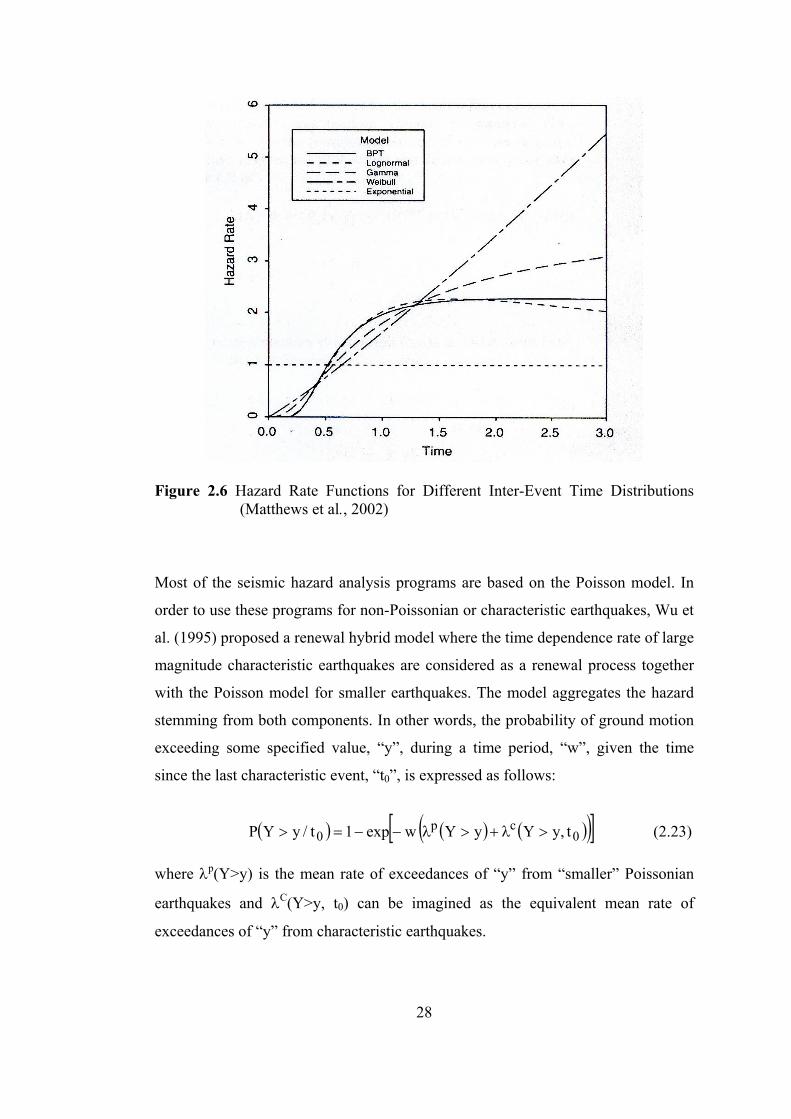
28
Figure 2.6 Hazard Rate Functions for Different Inter-Event Time Distributions (Matthews et al., 2002)
Most of the seismic hazard analysis programs are based on the Poisson model. In
order to use these programs for non-Poissonian or characteristic earthquakes, Wu et
al. (1995) proposed a renewal hybrid model where the time dependence rate of large
magnitude characteristic earthquakes are considered as a renewal process together
with the Poisson model for smaller earthquakes. The model aggregates the hazard
stemming from both components. In other words, the probability of ground motion
exceeding some specified value, “y”, during a time period, “w”, given the time
since the last characteristic event, “t0”, is expressed as follows:
( ) ( ) ( )( )[ ]0cp
0 t,yYyYwexp1t/yYP >λ+>λ−−=> (2.23) where λp(Y>y) is the mean rate of exceedances of “y” from “smaller” Poissonian
earthquakes and λC(Y>y, t0) can be imagined as the equivalent mean rate of
exceedances of “y” from characteristic earthquakes.

29
The mean rate of exceedances of “y” from Poissonian earthquakes can be written
as,
( ) [ ]earthquakesmallerone/yYP.yY pp >ν=>λ (2.24) where νP is the mean rate of the smaller earthquakes.
The equivalent mean rate of exceedances of “y” from characteristic earthquakes is
given as follows (Wu et al., 1995);
( ) [ ]dtearthquakesticcharacterioneyYP).t(hw1t,yY
wt
t0
C0
0
∫+
>=>λ (2.25)
The terms, P[Y>y/ one smaller earthquake] and P[Y>y/ one characteristic
earthquake] in Eqs. (2.24) and (2.25), are both time invariant. They can be
calculated by considering the relative likelihood of different magnitudes comprising
smaller or characteristic earthquakes, source to site distances and ground motion
estimation equations. Therefore, equivalent mean rate of characteristic earthquakes,
“νC(w,t0)”, can be calculated by using “η(w, t0)” which is given in Equation (2.22)
and is as follows;
( ) dt)t(F1
)t(fw1dt)t(h
w1
w)t,w(
t,wwt
t
wt
t
00
C0
0
0
0
∫∫++
−==
η=ν (2.26)
Since C)x(Fln)x(F)x(F
+=′
∫ , Eq. (2.26) becomes;
( ) ( ) ( )[ ]
⎟⎟⎟⎟⎟⎟
⎠
⎞
⎜⎜⎜⎜⎜⎜
⎝
⎛
−=−+−=ν
∫
∫∞
∞
+
0
0
t
wt000
C
dt).t(f
dt).t(f
lnw1)t(Gln)wt(Gln
w1t,w (2.27)

30
where G(⋅) is the complementary cumulative distribution function.
In regions that have relatively low seismicity and short earthquake histories, the
characteristic earthquakes may not be observed and do not appear in the earthquake
catalog. Therefore, the elapsed time since the last characteristic earthquake, “t0”,
can not be assessed. The only information on “t0” is that it is greater than the
temporal length of the available historical earthquake record, “L”. In this case, Wu
et al. (1995) proposed to replace “t0” in Eq. (2.25) by “L” and the hazard function
“h(t)” by “h+(t)” which is given as follows:
∫∞
+ =
tT
T
du)u(G
)t(G)t(h (2.28)
where GT(t) is the complementary cumulative distribution function of inter-event
times.
2.3.4 Attenuation Relationships (Ground Motion Prediction Equations) In seismic hazard analysis, ground motion attenuation relationships (ground motion
prediction equations) are the essential tools to estimate the ground motion
parameters at the site located at a distance from the source of an earthquake. When
an earthquake occurs, seismic waves and consequently ground motion will
propagate and attenuate with respect to distance away from its hypocenter,
depending on the soil conditions. The attenuation relationship gives an estimate of
ground motion parameter as a function of magnitude, distance from the site to the
epicenter (or hypocenter or to a selected point on the seismic source) and other
factors including type of faulting and local site conditions. Most of the attenuation
relationships are derived from the statistical analyses of the strong ground motion
records and they are updated as new records become available.

31
Although magnitude is the most acceptable scale of the earthquake severity, it can
not be directly used in earthquake resistant design of structures. Peak ground
acceleration (PGA), peak ground velocity (PGV) and 5 % damped elastic spectral
acceleration (SA) at various frequencies at a given site are the most common
parameters used in earthquake engineering. Until 1999 earthquakes, there were not
adequate numbers of ground motion records to develop a reliable ground motion
estimation equation for Turkey. Therefore, the attenuation relationships that were
developed for other countries were used for ground motion estimations for sites in
Turkey. Since 2002, a number of local attenuation models were developed based on
the data recorded in Turkey. The most commonly used recent attenuation
relationships are presented in the following sections.
2.3.4.1 Attenuation Models Developed for Other Countries The attenuation relationships that are believed to be consistent with the earthquake
mechanisms in our country and most widely used in seismic hazard studies carried
out for Turkey can be listed as (Yücemen et al., 2006):
• Abrahamson and Silva (1997)
• Boore et al. (1997)
• Sadigh et al. (1997)
• Ambraseys et al. (1996)
Each attenuation relationship is summarized in the following sections.
2.3.4.1.1 Abrahamson and Silva (1997) Abrahamson and Silva (1997) derived empirical response spectral attenuation
relationships for average horizontal and vertical components of shallow earthquakes
in active tectonic regions. The database used in the study consists of 655 recordings

32
from 58 earthquakes including Northridge earthquake. They classified the sites into
two categories: deep soil and rock or shallow soil. The general functional form of
the attenuation relationship is given as:
)agp(Sf)r,M(HWf)M(Ff)r,M(f)g(Saln rock5rup43rup1
)+++= (2.29) where;
Sa(g): spectral acceleration in g
M : moment magnitude
rrup : closest distance to the rupture plane in km
F : fault type (1for reverse, 0.5 for reverse/oblique and 0 otherwise)
HW : dummy variable for hanging wall sites (1 for sites over the hanging
wall, 0 otherwise)
S : dummy variable for the site class ( 0 for rock or shallow soil and 1 for
deep soil)
The function f1(M, rrup) is the basic functional form of the attenuation for strike-slip
events recorded at rock sites. For f1(M,rrup), the following form are used;
For M ≤ c1
[ ] Rln)cM(aa)M5.8(a)cM(aa)r,M(f 1133
n12121rup1 −++−+−+= (2.30)
For M > c1
[ ] Rln)cM(aa)M5.8(a)cM(aa)r,M(f 1133
n12141rup1 −++−+−+= (2.31)
where;
24
2rup crR += (2.32)
The function f3(M) that allows magnitude and period dependence of the style of
faulting factor is;

33
⎪⎪⎭
⎪⎪⎬
⎫
⎪⎪⎩
⎪⎪⎨
⎧
≥
<<−−
+
≤
=
16
11
565
5
3
cMfora
cM8.5for)8.5c()aa(
a
8.5Mfora
)M(f (2.33)
The functional form that takes into account the hanging wall effect, f4(M,rrup), is;
)r(f)M(f)r,M(f rupHWHWrup4 = (2.34) where;
⎪⎭
⎪⎬
⎫
⎪⎩
⎪⎨
⎧
≥<<−
≤=
5.6Mfor15.6M5.5for5.5M
5.5Mfor0)M(fHW (2.35)
and
⎪⎪⎪⎪⎪
⎭
⎪⎪⎪⎪⎪
⎬
⎫
⎪⎪⎪⎪⎪
⎩
⎪⎪⎪⎪⎪
⎨
⎧
>
<<⎟⎟⎠
⎞⎜⎜⎝
⎛ −−
<<
<<−
<
=
25rfor0
24r18for7
18r1a
18r8fora
8r4for4
4ra
4rfor0
)r(f
rup
ruprup
9
rup9
ruprup
9
rup
rupHW (2.36)
The nonlinear soil response is modeled by;
)cAGPln(aa)AGP(f 5rock1110rock5 ++=
)) (2.37)
where rockAGP
) is the expected peak acceleration on rock in g.
They gave following formula in order to calculate standard error in PGA and Sa
predictions;

34
⎪⎭
⎪⎬
⎫
≥<<
≤
⎪⎩
⎪⎨
⎧
−−−=σ
0.7Mfor0.7M0.5for
0.5Mfor
b2b)5M(bb
b)M(
65
65
5
total (2.38)
The coefficients were determined by using random effects model in which the
regression analysis was carried out in multiple steps and they are given for average
horizontal component in Table 2.3.
2.3.4.1.2 Boore et al. (1997) Boore et al. (1997) carried out a study on estimating peak horizontal acceleration
and random horizontal component of 5 percent damped pseudo acceleration
response spectra for shallow earthquakes in western North America.
They used moment magnitude as the measure of earthquake size and a distance
equal to the closest horizontal distance from the station to a point on the earth’s
surface that lies directly above the rupture. Shear wave velocity averaged over the
upper 30 m was used as a parameter to represent site effects. The ground motion
estimation equation is as follows:
A
sV5
2321 V
Vlnbrlnb)6M(b)6M(bbYln ++−+−+= (2.39)
where;
22jb hrr +=

35
Table 2.3 Coefficients for the Average Horizontal Component (Abrahamson and Silva, 1997)
Period c4 a1 a3 a5 a6 a9 a10 a11 a12 b5 b6
0.01 5.60 1.640 -1.1450 0.610 0.260 0.370 -0.417 -0.230 0.0000 0.70 0.135
0.02 5.60 1.640 -1.1450 0.610 0.260 0.370 -0.417 -0.230 0.0000 0.70 0.135
0.03 5.60 1.690 -1.1450 0.610 0.260 0.370 -0.470 -0.230 0.0143 0.70 0.135
0.04 5.60 1.780 -1.1450 0.610 0.260 0.370 -0.555 -0.251 0.0245 0.71 0.135
0.05 5.60 1.870 -1.1450 0.610 0.260 0.370 -0.620 -0.267 0.0280 0.71 0.135
0.06 5.60 1.940 -1.1450 0.610 0.260 0.370 -0.665 -0.280 0.0300 0.72 0.135
0.08 5.58 2.037 -1.1450 0.610 0.260 0.370 -0.628 -0.280 0.0300 0.73 0.135
0.09 5.54 2.100 -1.1450 0.610 0.260 0.370 -0.609 -0.280 0.0300 0.74 0.135
0.10 5.50 2.160 -1.1450 0.610 0.260 0.370 -0.598 -0.280 0.0280 0.74 0.135
0.12 5.39 2.272 -1.1450 0.610 0.260 0.370 -0.591 -0.280 0.0180 0.75 0.135
0.15 5.27 2.407 -1.1450 0.610 0.260 0.370 -0.577 -0.280 0.0050 0.75 0.135
0.17 5.19 2.430 -1.1350 0.610 0.260 0.370 -0.522 -0.265 -0.0040 0.76 0.135
0.20 5.10 2.406 -1.1150 0.610 0.260 0.370 -0.445 -0.245 -0.0138 0.77 0.135
0.24 4.97 2.293 -1.0790 0.610 0.232 0.370 -0.350 -0.223 -0.0238 0.77 0.135
0.30 4.80 2.114 -1.0350 0.610 0.198 0.370 -0.219 -0.195 -0.0360 0.78 0.135
0.36 4.62 1.955 -1.0052 0.610 0.170 0.370 -0.123 -0.173 -0.0460 0.79 0.135
0.40 4.52 1.860 -0.9880 0.610 0.154 0.370 -0.065 -0.160 -0.0518 0.79 0.135
0.46 4.38 1.717 -0.9652 0.592 0.132 0.370 0.020 -0.136 -0.0594 0.80 0.132
0.50 4.30 1.615 -0.9515 0.581 0.119 0.370 0.085 -0.121 -0.0635 0.80 0.130
0.60 4.12 1.428 -0.9218 0.557 0.091 0.370 0.194 -0.089 -0.0740 0.81 0.127
0.75 3.90 1.160 -0.8852 0.528 0.057 0.331 0.320 -0.050 -0.0862 0.81 0.123
0.85 3.81 1.020 -0.8648 0.512 0.038 0.309 0.370 -0.028 -0.0927 0.82 0.121
1.00 3.70 0.828 -0.8383 0.490 0.013 0.281 0.423 0.000 -0.1020 0.83 0.118
1.50 3.55 0.260 -0.7721 0.438 -0.049 0.210 0.600 0.040 -0.1200 0.84 0.110
2.00 3.50 -0.150 -0.7250 0.400 -0.094 0.160 0.610 0.040 -0.1400 0.85 0.105
3.00 3.50 -0.690 -0.7250 0.400 -0.156 0.089 0.630 0.040 -0.1726 0.87 0.097
4.00 3.50 -1.130 -0.7250 0.400 -0.200 0.039 0.640 0.040 -0.1956 0.88 0.092
5.00 3.50 -1.460 -0.7250 0.400 -0.200 0.000 0.664 0.040 -0.2150 0.89 0.087
Note: Other coefficients are; a2 = 0.512, a4 = -0.144, a13 = 0.17, c1 = 6.4, c5 = 0.03, n=2
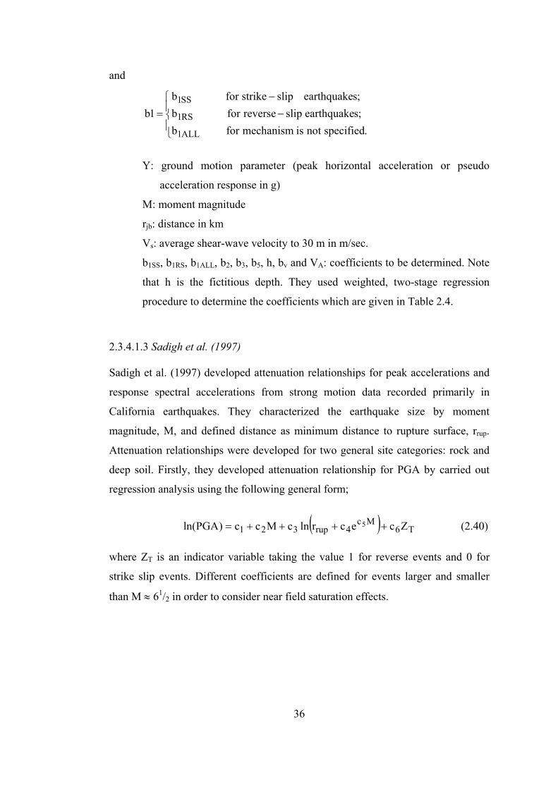
36
and
⎪⎩
⎪⎨
⎧−
−=
.specifiednotismechanismforb;searthquakeslipreverseforb;searthquakeslipstrikeforb
1b
ALL1
RS1
SS1
Y: ground motion parameter (peak horizontal acceleration or pseudo
acceleration response in g)
M: moment magnitude
rjb: distance in km
Vs: average shear-wave velocity to 30 m in m/sec.
b1SS, b1RS, b1ALL, b2, b3, b5, h, bv and VA: coefficients to be determined. Note
that h is the fictitious depth. They used weighted, two-stage regression
procedure to determine the coefficients which are given in Table 2.4.
2.3.4.1.3 Sadigh et al. (1997) Sadigh et al. (1997) developed attenuation relationships for peak accelerations and
response spectral accelerations from strong motion data recorded primarily in
California earthquakes. They characterized the earthquake size by moment
magnitude, M, and defined distance as minimum distance to rupture surface, rrup.
Attenuation relationships were developed for two general site categories: rock and
deep soil. Firstly, they developed attenuation relationship for PGA by carried out
regression analysis using the following general form;
( ) T6
Mc4rup321 ZcecrlncMcc)PGAln( 5 ++++= (2.40)
where ZT is an indicator variable taking the value 1 for reverse events and 0 for
strike slip events. Different coefficients are defined for events larger and smaller
than M ≈ 61/2 in order to consider near field saturation effects.

37
Table 2.4 Smoothed Coefficients for Pseudo-Acceleration Response Spectra (g) (Boore et al., 1997)
Period b1SS b1RV b1ALL b2 b3 b5 bv VA h σln(Y)
0.000 -0.313 -0.117 -0.242 0.527 0.000 -0.778 -0.371 1396 5.57 0.4950.100 1.006 1.087 1.059 0.753 -0.226 -0.934 -0.212 1112 6.27 0.4600.110 1.072 1.164 1.130 0.732 -0.230 -0.937 -0.211 1291 6.65 0.4590.120 1.109 1.215 1.174 0.721 -0.233 -0.939 -0.215 1452 6.91 0.4620.130 1.128 1.246 1.200 0.711 -0.233 -0.939 -0.221 1596 7.08 0.4610.140 1.135 1.261 1.208 0.707 -0.230 -0.938 -0.228 1718 7.18 0.4630.150 1.128 1.264 1.204 0.702 -0.228 -0.937 -0.238 1820 7.23 0.4640.160 1.112 1.257 1.192 0.702 -0.226 -0.935 -0.248 1910 7.24 0.4660.170 1.090 1.242 1.173 0.702 -0.221 -0.933 -0.258 1977 7.21 0.4670.180 1.063 1.222 1.151 0.705 -0.216 -0.930 -0.270 2037 7.16 0.4680.190 1.032 1.198 1.122 0.709 -0.212 -0.927 -0.281 2080 7.10 0.4690.200 0.999 1.170 1.089 0.711 -0.207 -0.924 -0.292 2118 7.02 0.4700.220 0.925 1.104 1.019 0.721 -0.198 -0.918 -0.315 2158 6.83 0.4740.240 0.847 1.033 0.941 0.732 -0.189 -0.912 -0.338 2178 6.62 0.4750.260 0.764 0.958 0.861 0.744 -0.180 -0.906 -0.360 2173 6.39 0.4770.280 0.681 0.881 0.780 0.758 -0.168 -0.899 -0.381 2158 6.17 0.4820.300 0.598 0.803 0.700 0.769 -0.161 -0.893 -0.401 2133 5.94 0.4840.320 0.518 0.725 0.619 0.783 -0.152 -0.888 -0.420 2104 5.72 0.4870.340 0.439 0.648 0.540 0.794 -0.143 -0.882 -0.438 2070 5.50 0.4910.360 0.361 0.570 0.462 0.806 -0.136 -0.877 -0.456 2032 5.30 0.4920.380 0.286 0.495 0.385 0.820 -0.127 -0.872 -0.472 1995 5.10 0.4970.400 0.212 0.423 0.311 0.831 -0.120 -0.867 -0.487 1954 4.91 0.4990.420 0.140 0.352 0.239 0.840 -0.113 -0.862 -0.502 1919 4.74 0.5020.440 0.073 0.282 0.169 0.852 -0.108 -0.858 -0.516 1884 4.57 0.5040.460 0.005 0.217 0.102 0.863 -0.101 -0.854 -0.529 1849 4.41 0.5080.480 -0.058 0.151 0.036 0.873 -0.097 -0.850 -0.541 1816 4.26 0.5100.500 -0.122 0.087 -0.025 0.884 -0.090 -0.846 -0.553 1782 4.13 0.5140.550 -0.268 -0.063 -0.176 0.907 -0.078 -0.837 -0.579 1710 3.82 0.5200.600 -0.401 -0.203 -0.314 0.928 -0.069 -0.830 -0.602 1644 3.57 0.5260.650 -0.523 -0.331 -0.440 0.946 -0.060 -0.823 -0.622 1592 3.36 0.5330.700 -0.634 -0.452 -0.555 0.962 -0.053 -0.818 -0.639 1545 3.20 0.5390.750 -0.737 -0.562 -0.661 0.979 -0.046 -0.813 -0.653 1507 3.07 0.5440.800 -0.829 -0.666 -0.760 0.992 -0.041 -0.809 -0.666 1476 2.98 0.5490.850 -0.915 -0.761 -0.851 1.006 -0.037 -0.805 -0.676 1452 2.92 0.5530.900 -0.993 -0.848 -0.933 1.018 -0.035 -0.802 -0.685 1432 2.89 0.5590.950 -1.066 -0.932 -1.010 1.027 -0.032 -0.800 -0.692 1416 2.88 0.5641.000 -1.133 -1.009 -1.080 1.036 -0.032 -0.798 -0.698 1406 2.90 0.5691.100 -1.249 -1.145 -1.208 1.052 -0.030 -0.795 -0.706 1396 2.99 0.5771.200 -1.345 -1.265 -1.315 1.064 -0.032 -0.794 -0.710 1400 3.14 0.5831.300 -1.428 -1.370 -1.407 1.073 -0.035 -0.793 -0.711 1416 3.36 0.5901.400 -1.495 -1.460 -1.483 1.080 -0.039 -0.794 -0.709 1442 3.62 0.5961.500 -1.552 -1.538 -1.550 1.085 -0.044 -0.796 -0.704 1479 3.92 0.6011.600 -1.598 -1.608 -1.605 1.087 -0.051 -0.798 -0.697 1524 4.26 0.6061.700 -1.634 -1.668 -1.652 1.089 -0.058 -0.801 -0.689 1581 4.62 0.6111.800 -1.663 -1.718 -1.689 1.087 -0.067 -0.804 -0.679 1644 5.01 0.6151.900 -1.685 -1.763 -1.720 1.087 -0.074 -0.808 -0.667 1714 5.42 0.6192.000 -1.699 -1.801 -1.743 1.085 -0.085 -0.812 -0.655 1795 5.85 0.622

38
Secondly, they performed analyses for spectral amplification (SA/PGA) by using
the following form;
( ) ( ) T6
Mc4rup9
5.287 ZcecrlncM5.8cc)PGA/SAln( 5 +++−+= (2.41)
Finally, they combined Eqs. (2.40) and (2.41) and smoothed parameters to obtain
attenuation relationships that predict smooth response spectra for earthquakes
having a moment magnitude from 4 and 8+ as well as at distances less than 100 km.
The attenuation model developed for rock is given as;
)2(rlnce(rlnc) - M5.8(cMccYln rup7
)Mc(crup4
5.2w3w21 w65 ++++++= + (2.42)
where;
Y : ground motion parameter (PGA, SA) in g
Mw : moment magnitude
rrup : the closest distance to the rupture surface in km
Note that in case of reverse/thrust faulting, the above strike-slip amplitudes are to be
multiplied by 1.2 for rock sites. The coefficients in Eq. (2.42) are given in Table 2.5
and Table 2.6 for Mw ≤ 6.5 and Mw > 6.5, respectively. Besides, Table 2.7 presents
dispersion relationships for horizontal rock motion.
Attenuation model proposed for deep soil site is given as follows;
5.2
w76·Mc
4rup3w21 )-M5.8(cc)ec(rlncMccYln w5 +++−+= (2.43) where;
Y : ground motion parameter (PGA, SA) in g
Mw : moment magnitude
rrup : the closest distance to the rupture surface in km
c1 = -2.17 for strike-slip, -1.92 for reverse and thrust earthquakes
c2 = 1.0
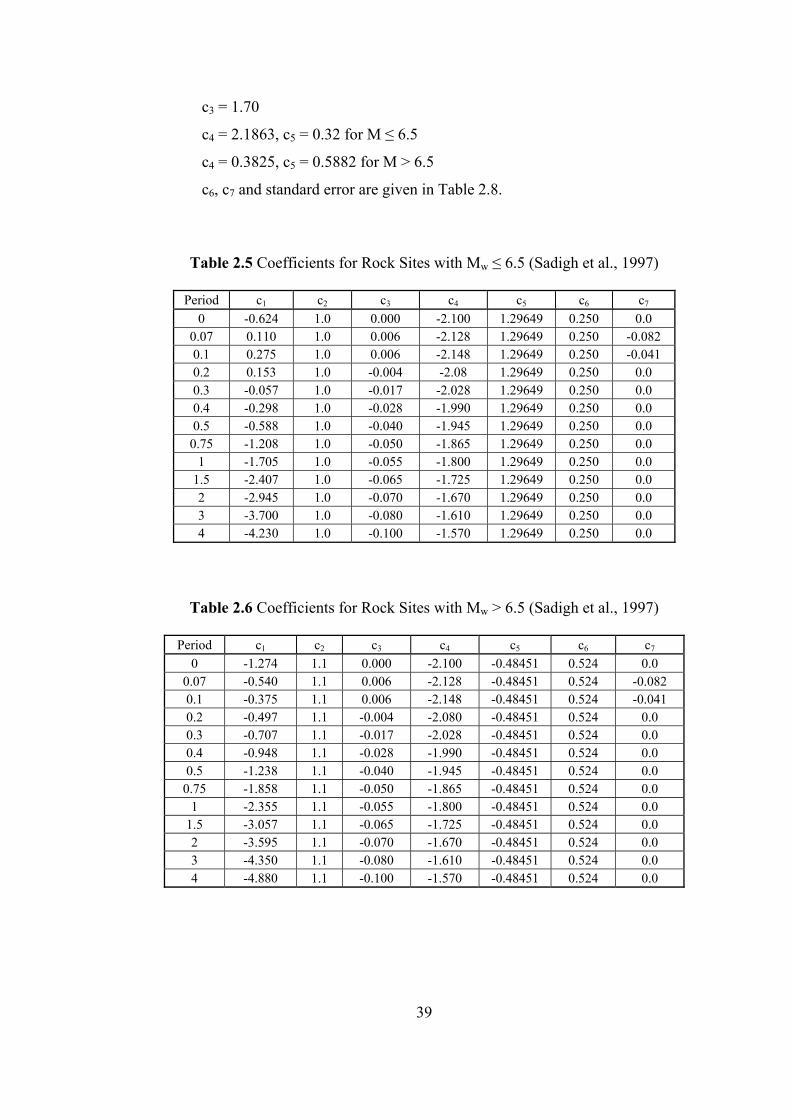
39
c3 = 1.70
c4 = 2.1863, c5 = 0.32 for M ≤ 6.5
c4 = 0.3825, c5 = 0.5882 for M > 6.5
c6, c7 and standard error are given in Table 2.8.
Table 2.5 Coefficients for Rock Sites with Mw ≤ 6.5 (Sadigh et al., 1997)
Period c1 c2 c3 c4 c5 c6 c7 0 -0.624 1.0 0.000 -2.100 1.29649 0.250 0.0
0.07 0.110 1.0 0.006 -2.128 1.29649 0.250 -0.082 0.1 0.275 1.0 0.006 -2.148 1.29649 0.250 -0.041 0.2 0.153 1.0 -0.004 -2.08 1.29649 0.250 0.0 0.3 -0.057 1.0 -0.017 -2.028 1.29649 0.250 0.0 0.4 -0.298 1.0 -0.028 -1.990 1.29649 0.250 0.0 0.5 -0.588 1.0 -0.040 -1.945 1.29649 0.250 0.0
0.75 -1.208 1.0 -0.050 -1.865 1.29649 0.250 0.0 1 -1.705 1.0 -0.055 -1.800 1.29649 0.250 0.0
1.5 -2.407 1.0 -0.065 -1.725 1.29649 0.250 0.0 2 -2.945 1.0 -0.070 -1.670 1.29649 0.250 0.0 3 -3.700 1.0 -0.080 -1.610 1.29649 0.250 0.0 4 -4.230 1.0 -0.100 -1.570 1.29649 0.250 0.0
Table 2.6 Coefficients for Rock Sites with Mw > 6.5 (Sadigh et al., 1997)
Period c1 c2 c3 c4 c5 c6 c7 0 -1.274 1.1 0.000 -2.100 -0.48451 0.524 0.0
0.07 -0.540 1.1 0.006 -2.128 -0.48451 0.524 -0.082 0.1 -0.375 1.1 0.006 -2.148 -0.48451 0.524 -0.041 0.2 -0.497 1.1 -0.004 -2.080 -0.48451 0.524 0.0 0.3 -0.707 1.1 -0.017 -2.028 -0.48451 0.524 0.0 0.4 -0.948 1.1 -0.028 -1.990 -0.48451 0.524 0.0 0.5 -1.238 1.1 -0.040 -1.945 -0.48451 0.524 0.0
0.75 -1.858 1.1 -0.050 -1.865 -0.48451 0.524 0.0 1 -2.355 1.1 -0.055 -1.800 -0.48451 0.524 0.0
1.5 -3.057 1.1 -0.065 -1.725 -0.48451 0.524 0.0 2 -3.595 1.1 -0.070 -1.670 -0.48451 0.524 0.0 3 -4.350 1.1 -0.080 -1.610 -0.48451 0.524 0.0 4 -4.880 1.1 -0.100 -1.570 -0.48451 0.524 0.0

40
Table 2.7 Dispersion Relationships for Horizontal Rock Motion (Sadigh et al., 1997)
Period σln(Y)
0 1.39-0.14M; 0.38 for M>7.21
0.07 1.40-0.14M; 0.39 for M>7.21
0.10 1.41-0.14M; 0.40 for M>7.21
0.20 1.43-0.14M; 0.42 for M>7.21
0.30 1.45-0.14M; 0.44 for M>7.21
0.40 1.48-0.14M; 0.47 for M>7.21
0.50 1.50-0.14M; 0.49 for M>7.21
0.75 1.52-0.14M; 0.51 for M>7.21
1.00 1.53-0.14M; 0.52 for M>7.21
>1.00 1.53-0.14M; 0.52 for M>7.21
Table 2.8 Coefficients for Deep Soil Sites (Sadigh et al., 1997)
Period c6 Strike-Slip c6 Reverse c7 Standard Error* 0 0.0 0.0 0.0 1.52-0.16M
0.075 0.4572 0.4572 0.005 1.54-0.16M
0.1 0.6395 0.6395 0.005 1.54-0.16M
0.2 0.9187 0.9187 -0.004 1.565-0.16M
0.3 0.9547 0.9547 -0.014 1.58-0.16M
0.4 0.9251 0.9005 -0.024 1.595-0.16M
0.5 0.8494 0.8285 -0.033 1.61-0.16M
0.75 0.7010 0.6802 -0.051 1.635-0.16M
1.0 0.5665 0.5075 -0.065 1.66-0.16M
1.5 0.3235 0.2215 -0.090 1.69-0.16M
2.0 0.1001 -0.0526 -0.108 1.7-0.16M
3.0 -0.2801 -0.4905 -0.139 1.71-0.16M
4.0 -0.6274 -0.8907 -0.160 1.71-0.16M * Standard error for M>7 set equal to the value for M=7.

41
2.3.4.1.4 Ambraseys et al. (1996) Ambraseys, et al. (1996) carried out a study in order to predict absolute spectral
acceleration ordinates in Europe and the Middle East. The database used in this
study consists of 422 triaxial records taken from 157 earthquakes in Europe and
adjacent areas (including Turkey) with magnitudes ranging from 4.0 and 7.9. As the
site to source distance, the closest distance to the projection of the fault rupture is
used. Four different site classes are defined based on shear wave velocity averaged
over the upper 30 m of the site, Vs: rock (Vs>750m/s); stiff soil
(360m/s<Vs≤750m/s); soft soil (180m/s<Vs≤360m/s); very soft soil (Vs≤180m/s).
Ambraseys et al. (1996) proposed the relationship given in Eq. (2.44) with the
coefficients presented in Table 2.9.
PSCSChdlogCMCC(Y)log SSAA20
24s21 σ++++++′= (2.44)
In Eq. (2.44), Y is the ground motion parameter (PGA, SA) in g; Ms is surface
magnitude; d is the shortest distance to the projection of fault rupture, in km; h0,
C1′, C2 and C4 are constants given in Table 2.9. σ is the standard deviation of log
(y) and the constant P takes a value of 0 for mean values and 1 for 84-percentile
values of log (Y). SA and SS account for the soil and soft soil types taking values
given below:
Rock (Vs>750m/s): SA=0, SS=0
Stiff soil (360m/s<Vs≤750m/s): SA=1, SS=0
Soft soil (180m/s<Vs≤360m/s): SA=0, SS=1
Very soft soil (Vs≤180m/s): SA=0, SS=1

42
Table 2.9 Coefficients of the Attenuation Relationship Proposed by Ambraseys et al. (1996)
Period(sec) C1' C2 h0 C4 CA CS σ
0.10 -0.84 0.219 4.5 -0.954 0.078 0.027 0.27 0.11 -0.86 0.221 4.5 -0.945 0.098 0.036 0.27 0.12 -0.87 0.231 4.7 -0.960 0.111 0.052 0.27 0.13 -0.87 0.238 5.3 -0.981 0.131 0.068 0.27 0.14 -0.94 0.244 4.9 -0.955 0.136 0.077 0.27 0.15 -0.98 0.247 4.7 -0.938 0.143 0.085 0.27 0.16 -1.05 0.252 4.4 -0.907 0.152 0.101 0.27 0.17 -1.08 0.258 4.3 -0.896 0.140 0.102 0.27 0.18 -1.13 0.268 4.0 -0.901 0.129 0.107 0.27 0.19 -1.19 0.278 3.9 -0.907 0.133 0.130 0.28 0.20 -1.21 0.284 4.2 -0.922 0.135 0.142 0.27 0.22 -1.28 0.295 4.1 -0.911 0.120 0.143 0.28 0.24 -1.37 0.308 3.9 -0.916 0.124 0.155 0.28 0.26 -1.40 0.318 4.3 -0.942 0.134 0.163 0.28 0.28 -1.46 0.326 4.4 -0.946 0.134 0.158 0.29 0.30 -1.55 0.338 4.2 -0.933 0.133 0.148 0.30 0.32 -1.63 0.349 4.2 -0.932 0.125 0.161 0.31 0.34 -1.65 0.351 4.4 -0.939 0.118 0.163 0.31 0.36 -1.69 0.354 4.5 -0.936 0.124 0.160 0.31 0.38 -1.82 0.364 3.9 -0.900 0.132 0.164 0.31 0.40 -1.94 0.377 3.6 -0.888 0.139 0.172 0.31 0.42 -1.99 0.384 3.7 -0.897 0.147 0.180 0.32 0.44 -2.05 0.393 3.9 -0.908 0.153 0.187 0.32 0.46 -2.11 0.401 3.7 -0.911 0.149 0.191 0.32 0.48 -2.17 0.410 3.5 -0.920 0.150 0.197 0.32 0.50 -2.25 0.420 3.3 -0.913 0.147 0.201 0.32 0.55 -2.38 0.434 3.1 -0.911 0.134 0.203 0.32 0.60 -2.49 0.438 2.5 -0.881 0.124 0.212 0.32 0.65 -2.58 0.451 2.8 -0.901 0.122 0.215 0.32 0.70 -2.67 0.463 3.1 -0.914 0.116 0.214 0.33 0.75 -2.75 0.477 3.5 -0.942 0.113 0.212 0.32 0.80 -2.86 0.485 3.7 -0.925 0.127 0.218 0.32 0.85 -2.93 0.492 3.9 -0.920 0.124 0.218 0.32 0.90 -3.03 0.502 4.0 -0.920 0.124 0.225 0.32 0.95 -3.10 0.503 4.0 -0.892 0.121 0.217 0.32 1.00 -3.17 0.508 4.3 -0.885 0.128 0.219 0.32 1.10 -3.30 0.513 4.0 -0.857 0.123 0.206 0.32 1.20 -3.38 0.513 3.6 -0.851 0.128 0.214 0.31 1.30 -3.43 0.514 3.6 -0.848 0.115 0.200 0.31 1.40 -3.52 0.522 3.4 -0.839 0.109 0.197 0.31 1.50 -3.61 0.524 3.0 -0.817 0.109 0.204 0.31 1.60 -3.68 0.520 2.5 -0.781 0.108 0.206 0.31 1.70 -3.74 0.517 2.5 -0.759 0.105 0.206 0.31 1.80 -3.79 0.514 2.4 -0.730 0.104 0.204 0.32 1.90 -3.80 0.508 2.8 -0.724 0.103 0.194 0.32 2.00 -3.79 0.503 3.2 -0.728 0.101 0.182 0.32

43
2.3.4.2 Attenuation Models Developed for Turkey
After two destructive earthquakes occurred in 1999 in Turkey, there has been an
increase in the strong ground motion data. Therefore, researchers have been
encouraged to develop local attenuation relationships for Turkey. In 2002, Gülkan
and Kalkan (2002) compiled a database that contains 93 records from 47 horizontal
components of 19 earthquakes that occurred between 1976 and 1999 in Turkey.
They derived a set of empirical attenuation relationships to estimate free field
horizontal components of peak ground acceleration and 5 percent damped pseudo
acceleration response by using this database. In 2004, they updated this database
and accordingly revised the relationship. Also, other researchers, Özbey et al.
(2004) and Ulusay et al. (2004), developed attenuation models from the recorded
ground motions in Turkey. In addition to these recent relationships, there are other
attenuation relationships suggested by İnan et al. (1996), Aydan et al. (1996) and
Aydan (2001) for Turkey. These relationships will be briefly explained in the
following sections.
2.3.4.2.1 İnan et al. (1996) İnan et al. (1996) developed the following equation for peak ground acceleration
(PGA);
44.0Rlog9.0M65.0PGAlog −−= (2.45) where M is the earthquake magnitude and R is the distance to epicenter in
kilometers. It should be noted that this relationship gives too conservative PGA
values particularly in near source areas (Ulusay et al., 2004).
2.3.4.2.2 Aydan et al. (1996) and Aydan ( 2001) The attenuation relationship developed by Aydan et al. (1996) is given in the
following form:

44
( )1ee8.2a R025.0Ms9.0max −= − (2.46)
where amax is the maximum ground acceleration; Ms and R are the surface wave
magnitude and the hypocentral distance of a given earthquake, respectively.
Aydan (2001) modified the attenuation equation suggested by Aydan et al. (1996)
as follows:
( )1ee8.2a Ms9.0R025.0
max −= − (2.47) 2.3.4.2.3 Gülkan and Kalkan (2002), Kalkan and Gülkan (2004) Gülkan and Kalkan (2002) derived a set of empirical attenuation relationships to
estimate free field horizontal components of peak ground acceleration and 5 percent
damped pseudo acceleration response by using a strong ground motion database
which contains 93 records from 47 horizontal components of 19 earthquakes that
occurred between 1976 and 1999 in Turkey.
They used same definitions of predictory variables; i.e. earthquake size, site-to
source distance and site condition parameter; and same general form of the ground
motion estimation equation with Boore et al. (1997). Since actual shear wave
velocities and detailed site description were not available for most of the stations,
they divided site conditions in Turkey into three groups; soft soil, soil and rock; and
they assigned shear wave velocities of 200, 400 and 700 m/s to these groups,
respectively.
Gülkan and Kalkan (2002) applied nonlinear regression procedure to determine
unknown coefficients in Eq. 2.39 and they are given in Table 2.10.
In 2004, they expanded and updated the database. This new database consists of
112 strong ground motion records of 57 earthquakes that occurred between 1976
and 2003. The coefficients estimated by Kalkan and Gülkan (2004) by using this
updated database are given in Table 2.11.

45
Table 2.10 Coefficients of Attenuation Relationships Developed by Gülkan and Kalkan (2002)
Period (sec) b1 b2 b3 b5 bV VA h σln(Y)
0 (PGA) –0.682 0.253 0.036 –0.562 –0.297 1381 4.48 0.562 0.10 –0.139 0.200 –0.003 –0.553 –0.167 1063 3.76 0.621 0.11 0.031 0.235 –0.007 –0.573 –0.181 1413 3.89 0.618 0.12 0.123 0.228 –0.031 –0.586 –0.208 1501 4.72 0.615 0.13 0.138 0.216 –0.007 –0.590 –0.237 1591 5.46 0.634 0.14 0.100 0.186 0.014 –0.585 –0.249 1833 4.98 0.635 0.15 0.090 0.210 –0.013 –0.549 –0.196 1810 2.77 0.620 0.16 –0.128 0.214 0.007 –0.519 –0.224 2193 1.32 0.627 0.17 –0.107 0.187 0.037 –0.535 –0.243 2433 1.67 0.621 0.18 0.045 0.168 0.043 –0.556 –0.256 2041 2.44 0.599 0.19 0.053 0.180 0.063 –0.570 –0.288 2086 2.97 0.601 0.20 0.127 0.192 0.065 –0.597 –0.303 2238 3.48 0.611 0.22 –0.081 0.214 0.006 –0.532 –0.319 2198 1.98 0.584 0.24 –0.167 0.265 –0.035 –0.531 –0.382 2198 2.55 0.569 0.26 –0.129 0.345 –0.039 –0.552 –0.395 2160 3.45 0.549 0.28 0.140 0.428 –0.096 –0.616 –0.369 2179 4.95 0.530 0.30 0.296 0.471 –0.140 –0.642 –0.346 2149 6.11 0.540 0.32 0.454 0.476 –0.168 –0.653 –0.290 2144 7.38 0.555 0.34 0.422 0.471 –0.152 –0.651 –0.300 2083 8.30 0.562 0.36 0.554 0.509 –0.114 –0.692 –0.287 2043 9.18 0.563 0.38 0.254 0.499 –0.105 –0.645 –0.341 2009 9.92 0.562 0.40 0.231 0.497 –0.105 –0.647 –0.333 1968 9.92 0.604 0.42 0.120 0.518 –0.135 –0.612 –0.313 1905 9.09 0.634 0.44 0.035 0.544 –0.142 –0.583 –0.286 1899 9.25 0.627 0.46 –0.077 0.580 –0.147 –0.563 –0.285 1863 8.98 0.642 0.48 –0.154 0.611 –0.154 –0.552 –0.293 1801 8.96 0.653 0.50 –0.078 0.638 –0.161 –0.565 –0.259 1768 9.06 0.679 0.55 –0.169 0.707 –0.179 –0.539 –0.216 1724 8.29 0.710 0.60 –0.387 0.698 –0.187 –0.506 –0.259 1629 8.24 0.707 0.65 –0.583 0.689 –0.159 –0.500 –0.304 1607 7.64 0.736 0.70 –0.681 0.698 –0.143 –0.517 –0.360 1530 7.76 0.743 0.75 –0.717 0.730 –0.143 –0.516 –0.331 1492 7.12 0.740 0.80 –0.763 0.757 –0.113 –0.525 –0.302 1491 6.98 0.742 0.85 –0.778 0.810 –0.123 –0.529 –0.283 1438 6.57 0.758 0.90 –0.837 0.856 –0.130 –0.512 –0.252 1446 7.25 0.754 0.95 –0.957 0.870 –0.127 –0.472 –0.163 1384 7.24 0.752 1.00 –1.112 0.904 –0.169 –0.443 –0.200 1391 6.63 0.756 1.10 –1.459 0.898 –0.147 –0.414 –0.252 1380 6.21 0.792 1.20 –1.437 0.962 –0.156 –0.463 –0.267 1415 7.17 0.802 1.30 –1.321 1.000 –0.147 –0.517 –0.219 1429 7.66 0.796 1.40 –1.212 1.000 –0.088 –0.584 –0.178 1454 9.10 0.790 1.50 –1.340 0.997 –0.055 –0.582 –0.165 1490 9.86 0.788 1.60 –1.353 0.999 –0.056 –0.590 –0.135 1513 9.94 0.787 1.70 –1.420 0.996 –0.052 –0.582 –0.097 1569 9.55 0.789 1.80 –1.465 0.995 –0.053 –0.581 –0.058 1653 9.35 0.827 1.90 –1.500 0.999 –0.051 –0.592 –0.047 1707 9.49 0.864 2.00 –1.452 1.020 –0.079 –0.612 –0.019 1787 9.78 0.895

46
Table 2.11 Coefficients of Attenuation Relationships Developed by Kalkan and Gülkan (2004)
Period (sec) b1 b2 b3 b5 bv VA h
σln(Y)
PGA 0.393 0.576 -0.107 -0.899 -0.200 1112 6.91 0.612 0.10 1.796 0.441 -0.087 -1.023 -0.054 1112 10.07 0.658 0.11 1.627 0.498 -0.086 -1.030 -0.051 1290 10.31 0.643 0.12 1.109 0.721 -0.233 -0.939 -0.215 1452 6.91 0.650 0.13 1.474 0.500 -0.127 -1.070 -0.300 1953 10.00 0.670 0.14 0.987 0.509 -0.114 -1.026 -0.500 1717 9.00 0.620 0.15 1.530 0.511 -0.127 -1.070 -0.300 1953 10.00 0.623 0.16 1.471 0.517 -0.125 -1.052 -0.298 1954 9.59 0.634 0.17 1.500 0.530 -0.115 -1.060 -0.297 1955 9.65 0.651 0.18 1.496 0.547 -0.115 -1.060 -0.301 1957 9.40 0.646 0.19 1.468 0.575 -0.108 -1.055 -0.302 1958 9.23 0.657 0.20 1.419 0.597 -0.097 -1.050 -0.303 1959 8.96 0.671 0.22 0.989 0.628 -0.118 -0.951 -0.301 1959 6.04 0.683 0.24 0.736 0.654 -0.113 -0.892 -0.302 1960 5.16 0.680 0.26 0.604 0.696 -0.109 -0.860 -0.305 1961 4.70 0.682 0.28 0.727 0.733 -0.127 -0.891 -0.303 1963 5.74 0.674 0.30 0.799 0.751 -0.148 -0.909 -0.297 1964 6.49 0.720 0.32 0.749 0.744 -0.161 -0.897 -0.300 1954 7.18 0.714 0.34 0.798 0.741 -0.154 -0.891 -0.266 1968 8.10 0.720 0.36 0.589 0.752 -0.143 -0.867 -0.300 2100 7.90 0.650 0.38 0.490 0.763 -0.138 -0.852 -0.300 2103 8.00 0.779 0.40 0.530 0.775 -0.147 -0.855 -0.264 2104 8.32 0.772 0.42 0.353 0.784 -0.150 -0.816 -0.267 2104 7.69 0.812 0.44 0.053 0.782 -0.132 -0.756 -0.268 2103 7.00 0.790 0.46 0.049 0.780 -0.157 -0.747 -0.290 2059 7.30 0.781 0.48 -0.170 0.796 -0.153 -0.704 -0.275 2060 6.32 0.789 0.50 -0.146 0.828 -0.161 -0.710 -0.274 2064 6.22 0.762 0.55 -0.306 0.866 -0.156 -0.702 -0.292 2071 5.81 0.808 0.60 -0.383 0.881 -0.179 -0.697 -0.303 2075 6.13 0.834 0.65 -0.491 0.896 -0.182 -0.696 -0.300 2100 5.80 0.845 0.70 -0.576 0.914 -0.190 -0.681 -0.301 2102 5.70 0.840 0.75 -0.648 0.933 -0.185 -0.676 -0.300 2104 5.90 0.828 0.80 -0.713 0.968 -0.183 -0.676 -0.301 2090 5.89 0.839 0.85 -0.567 0.986 -0.214 -0.695 -0.333 1432 6.27 0.825 0.90 -0.522 1.019 -0.225 -0.708 -0.313 1431 6.69 0.826 0.95 -0.610 1.050 -0.229 -0.697 -0.303 1431 6.89 0.841 1.00 -0.662 1.070 -0.250 -0.696 -0.305 1405 6.89 0.874 1.10 -1.330 1.089 -0.255 -0.684 -0.500 2103 7.00 0.851 1.20 -1.370 1.120 -0.267 -0.690 -0.498 2103 6.64 0.841 1.30 -1.474 1.155 -0.269 -0.696 -0.496 2103 6.00 0.856 1.40 -1.665 1.170 -0.258 -0.674 -0.500 2104 5.44 0.845 1.50 -1.790 1.183 -0.262 -0.665 -0.501 2104 5.57 0.840 1.60 -1.889 1.189 -0.265 -0.662 -0.503 2102 5.50 0.834 1.70 -1.968 1.200 -0.272 -0.664 -0.502 2101 5.30 0.828 1.80 -2.037 1.210 -0.284 -0.666 -0.505 2098 5.10 0.849 1.90 -1.970 1.210 -0.295 -0.675 -0.501 1713 5.00 0.855 2.00 -2.110 1.200 -0.300 -0.663 -0.499 1794 4.86 0.878

47
2.3.4.2.4 Özbey et al. (2004) The study conducted by Özbey et al. (2004) resulted in empirical attenuation
relationships for horizontal peak ground acceleration and 5 percent spectral
acceleration. They used a database that contains 195 recordings from 17
earthquakes including Kocaeli and Düzce earthquakes in addition to their
aftershocks and other events. Earthquake size was defined in terms of moment
magnitude and the site to source distance was taken as the closest horizontal
distance to the vertical projection of the rupture plane. Sites were divided into 4
classes according to their shear wave velocities. Site class definitions are shown in
Table 2.12.
They used following empirical attenuation model:
2122
ij2
iiij fGeGhRlogd)6M(c)6M(ba)Y(log ++++−+−+= (2.48)
where;
Yij: geometric mean of the two horizontal components of the ground motion
parameter in cm/s2 from the jth recording of the ith event
Mi: moment magnitude of ith event
Rij: closest horizontal distance to the vertical projection of the rupture from
ith event to the location of jth recording.
The coefficients G1 and G2 take on values as follows;
G1=0 and G2=0 for site classes A and B
G1=1 and G2=0 for site class C
G1=0 and G2=1 for site class D.

48
Table 2.12 Site Class Definitions Used by Özbey et al. (2004)
Site Class Shear Wave VelocityA >750 m/s B 360-750 m/s C 180-360 m/s D <180m/s
The coefficients a, b, c, d, e, f and h were estimated by using mixed effect model in
which some of the attenuation model coefficients were modeled as random and
others as fixed. These coefficients are given in Table 2.13.
2.3.4.2.5 Ulusay et al. (2004) Ulusay et al. (2004) carried out a study in which a local attenuation relationship for
peak ground acceleration (PGA) was developed by using 221 records from 122
earthquakes that occurred between 1976 and 2003 in Turkey. Moment magnitude
was used to define earthquake size and epicentral distance was as site to source
distance. Nonlinear regression method was applied to obtain an attenuation
relationship for PGA.
They proposed the following relationship to predict PGA;
)S9282.18S8427.7RM3.33(0218.0 BAewe18.2PGA ++−= (2.49) where;
PGA: peak ground acceleration in gal
Mw: moment magnitude
Re: distance to epicenter in km
The terms to include site conditions, SA and SB, take on following values;
SA=0 and SB=0 for rock sites
SA=1 and SB=0 for soil sites
SA=0 and SB=1 for soft soil sites.

49
Table 2.13 Attenuation Coefficients in the Equation Proposed by Özbey et al. (2004)
Period (sec) a b c d h e f
σlog Y
PGA 3.287 0.503 -0.079 -1.1177 14.82 0.141 0.331 0.260 0.10 3.755 0.419 -0.052 -1.3361 17.22 0.173 0.255 0.274 0.15 3.922 0.463 -0.085 -1.3422 21.41 0.182 0.268 0.266 0.20 3.518 0.494 -0.094 -1.1162 14.87 0.113 0.285 0.243 0.25 3.270 0.517 -0.099 -0.9781 9.75 0.053 0.288 0.250 0.30 3.040 0.549 -0.095 -0.8762 6.54 0.062 0.320 0.262 0.35 2.951 0.579 -0.121 -0.8402 6.48 0.080 0.352 0.267 0.40 2.825 0.593 -0.112 -0.8089 6.48 0.102 0.394 0.281 0.45 2.690 0.605 -0.111 -0.7572 6.17 0.105 0.408 0.289 0.50 2.685 0.653 -0.171 -0.7302 5.58 0.051 0.385 0.293 0.55 2.581 0.685 -0.177 -0.6928 3.56 0.061 0.393 0.306 0.60 2.423 0.708 -0.177 -0.6291 3.41 0.059 0.399 0.302 0.65 2.325 0.724 -0.177 -0.6032 2.50 0.063 0.411 0.303 0.70 2.276 0.741 -0.174 -0.5932 2.12 0.055 0.407 0.300 0.75 2.247 0.750 -0.170 -0.5946 2.34 0.054 0.396 0.305 0.80 2.247 0.755 -0.166 -0.6075 3.22 0.070 0.392 0.307 0.85 2.243 0.774 -0.161 -0.6353 3.22 0.094 0.407 0.315 0.90 2.272 0.791 -0.172 -0.6630 4.21 0.102 0.416 0.324 0.95 2.246 0.807 -0.182 -0.6570 4.23 0.099 0.414 0.328 1.00 2.237 0.828 -0.207 -0.6543 4.14 0.100 0.413 0.331 1.10 2.227 0.855 -0.248 -0.6616 3.78 0.113 0.415 0.334 1.20 2.267 0.874 -0.267 -0.6910 4.49 0.103 0.397 0.330 1.30 2.353 0.901 -0.284 -0.7516 5.35 0.092 0.394 0.339 1.40 2.376 0.932 -0.296 -0.7752 6.90 0.070 0.375 0.349 1.50 2.445 0.943 -0.314 -0.8117 7.73 0.045 0.328 0.357 1.75 2.466 0.964 -0.331 -0.8671 7.85 0.038 0.298 0.364 2.00 2.490 0.973 -0.331 -0.9397 8.55 0.059 0.301 0.353 2.25 2.581 0.977 -0.326 -1.0345 11.21 0.070 0.299 0.347 2.75 2.559 0.980 -0.282 -1.1235 11.68 0.060 0.286 0.323 3.00 2.564 0.998 -0.282 -1.1473 12.04 0.044 0.273 0.324 3.50 2.549 1.011 -0.278 -1.1950 10.93 0.044 0.261 0.329 4.00 2.366 1.028 -0.244 -1.1710 10.72 0.025 0.253 0.324

50
2.3.5 Seismic Hazard Calculations The probability of exceedance of a specified ground motion level is obtained by
calculating the contribution of each seismic source independently and aggregating
them based on the theorem of total probability. In order to construct a seismic
hazard curve for a specific site, a set of ground motion values are selected and the
annual frequency of the ground motion parameter, Y, exceeding each ground
motion value, y, is calculated from the following expression:
( ) dx)X(f)X/yY(Pr...yY
~x
iSources ~i∑ ∫∫ ∫ ≥ν=≥λ (2.50)
where; νi is the annual rate of occurrence of earthquakes on seismic source i;
~X is
the vector of random variables that influence Y and fx(~X ) is the joint probability
density function of ~X . Generally, random variables in
~X are the magnitude, M,
and distance, R. Assuming that these variables are independent, the annual
frequency of exceedance, λ(Y ≥ y), can be written as;
( ) [ ] drdm)r(f)m(fR,MyYPryY
iRiMiiSourcesi∑ ∫∫ ≥ν=≥λ (2.51)
where fMi(m) and fRi(r) are the probability density functions of magnitude and
distance for source i, respectively.
It is too difficult to evaluate the integrals in Eq. (2.51) analytically. Therefore, in
practice, earthquake magnitude distribution is discretized by dividing the possible
range of magnitudes into small intervals. Then, center of each interval, denoted as
Mj, is used in calculations. The possible locations of each earthquake magnitude,
Mj, are also discretized by distance Rk. Therefore, a set of earthquake scenarios with
magnitude, Mj, occurring at a distance of Rk from the site of interest are defined.
For each scenario, the annual earthquake occurrence rate, ν(j,k), is calculated based
on probability distributions of earthquake magnitude and ruptures. Then the annual
frequency of exceedance, λ(Y ≥ y), is calculated from;

51
( ) [ ]∑ ∑ ∑ ≥ν=≥λiSources jMagnitudes kcestanDis
kj R,MyYPr)k,j(yY (2.52)
Note that conditional probability; P[Y≥y/Mj, Rk]; is computed by considering the
uncertainty in the ground motion parameter predicted from the attenuation
relationship as will be explained in Section 2.3.6.1.
2.3.6 Consideration of Uncertainties PSHA accounts for uncertainties associated with randomness in various input
parameters describing seismicity and modeling of ground motion attenuation.
Uncertainties in PSHA are divided into two types: aleatory and epistemic. Aleatory
uncertainty is the inherent variability due to unpredictable nature of future events.
In other words, this is the uncertainty in the data used in the analysis and
randomness related with prediction of a parameter from a specific model, assuming
that the model is correct (Thenhaus and Campbell, 2003). On the other hand,
epistemic or modeling uncertainty results from incomplete knowledge in the
predictive models and variability in the interpretations of the data used to develop
the models (Thenhaus and Campbell, 2003). This type of uncertainties can be
reduced as more data are collected, more information acquired and more research
completed. Some examples of uncertainties in PSHA are presented in Table 2.14. In
PSHA, the aleatory uncertainties in the parameters are described by suitable
probability distributions and are included directly into calculations by quantifying
the appropriate statistical parameters (i.e., standard deviation, coefficient of
variation). Epistemic uncertainty is considered by including alternative models and
aggregating them through logic tree methodology.
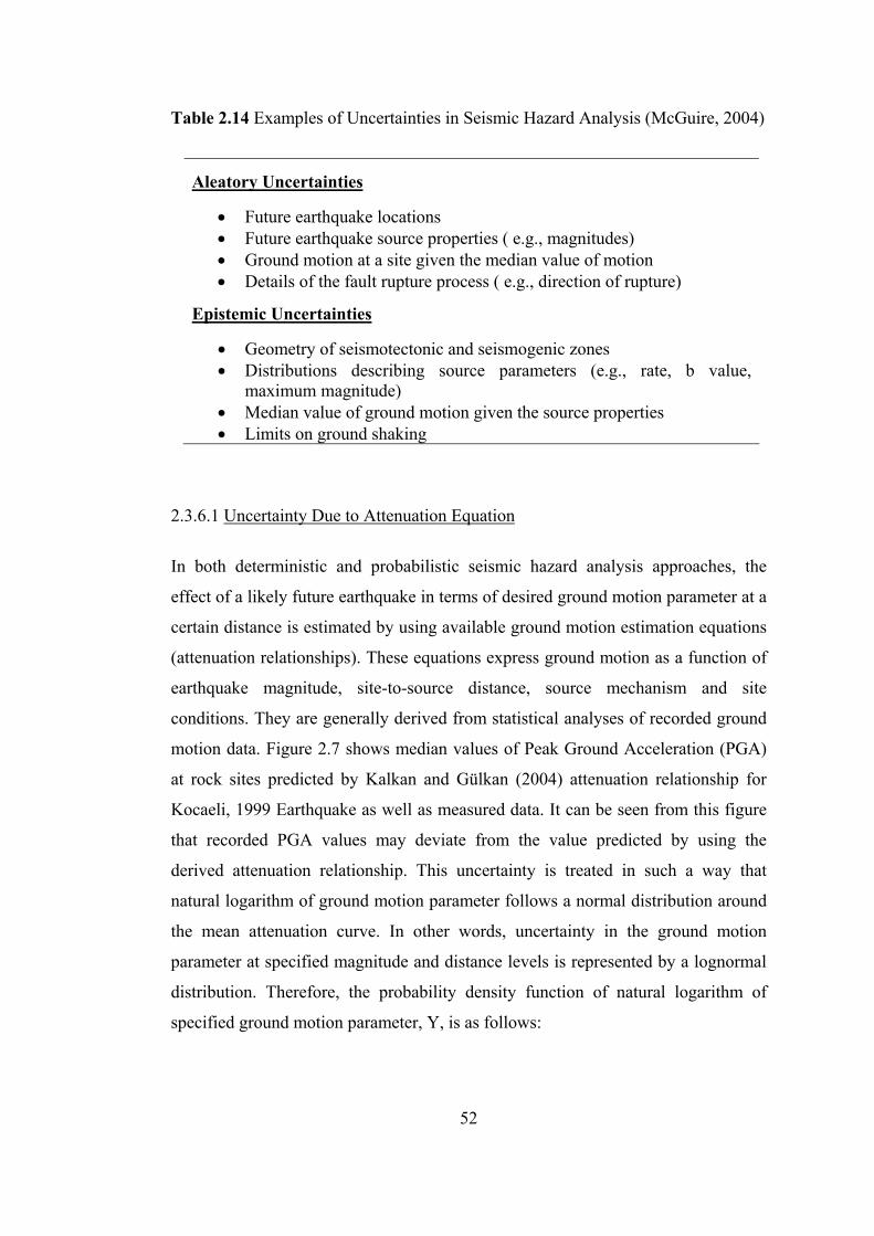
52
Table 2.14 Examples of Uncertainties in Seismic Hazard Analysis (McGuire, 2004)
Aleatory Uncertainties
• Future earthquake locations • Future earthquake source properties ( e.g., magnitudes) • Ground motion at a site given the median value of motion • Details of the fault rupture process ( e.g., direction of rupture)
Epistemic Uncertainties
• Geometry of seismotectonic and seismogenic zones • Distributions describing source parameters (e.g., rate, b value,
maximum magnitude) • Median value of ground motion given the source properties • Limits on ground shaking
2.3.6.1 Uncertainty Due to Attenuation Equation
In both deterministic and probabilistic seismic hazard analysis approaches, the
effect of a likely future earthquake in terms of desired ground motion parameter at a
certain distance is estimated by using available ground motion estimation equations
(attenuation relationships). These equations express ground motion as a function of
earthquake magnitude, site-to-source distance, source mechanism and site
conditions. They are generally derived from statistical analyses of recorded ground
motion data. Figure 2.7 shows median values of Peak Ground Acceleration (PGA)
at rock sites predicted by Kalkan and Gülkan (2004) attenuation relationship for
Kocaeli, 1999 Earthquake as well as measured data. It can be seen from this figure
that recorded PGA values may deviate from the value predicted by using the
derived attenuation relationship. This uncertainty is treated in such a way that
natural logarithm of ground motion parameter follows a normal distribution around
the mean attenuation curve. In other words, uncertainty in the ground motion
parameter at specified magnitude and distance levels is represented by a lognormal
distribution. Therefore, the probability density function of natural logarithm of
specified ground motion parameter, Y, is as follows:

53
⎥⎥
⎦
⎤
⎢⎢
⎣
⎡
⎟⎟⎠
⎞⎜⎜⎝
⎛
σ−
−σπ
=2
YlnYlnY
)r,m(Yln)y(ln21exp
21)y(f (2.53)
where; y is the ground motion level of interest; )r,m(Yln is the mean value of
natural logarithm of ground motion caused by an earthquake with magnitude, m,
occurred at a distance, r, to the site and σln Y is the standard deviation of ln Y.
Figure 2.8 (a) shows the visual description of Eq. (2.53).
Figure 2.7 Median Peak Ground Acceleration (PGA) Curve Predicted for Kocaeli,
1999 Earthquake by Using Kalkan and Gülkan (2004) Attenuation Relationship at Rock Sites; Distribution of PGA Values at 1 km Distance and the Recorded Data
After the classical PSHA model was introduced, this uncertainty has been
incorporated into the analysis directly. Therefore, the annual probability of ground
motion parameter exceeding a specified level is determined not only by its median
value but also by its standard deviation. In PSHA, for each earthquake scenario the
probability of exceeding a specified ground motion level, y, is calculated by
integrating Eq. (2.53) as shown by Eq. (2.54).
0.01
0.1
1
10
1 10 100
Closest Distance (km)
PGA
(g)
Median Attenuation Curve
Recorded Data at Kocaeli, 1999 Earthquake
Distribution of predicted PGA values at 1 km

54
ylnd)r,m(Yln)y(ln21exp
21)yYPr(
yln
2
YlnYln∫∞
⎥⎥
⎦
⎤
⎢⎢
⎣
⎡
⎟⎟⎠
⎞⎜⎜⎝
⎛
σ−
−σπ
=> (2.54)
For each ground motion level, the probability given in Eq. (2.54) is calculated and
then it is plotted to obtain a hazard curve like the one shown in Figure 2.8 (b). This
curve actually shows the complementary cumulative distribution function of a
selected ground motion parameter. For an assumed earthquake scenario, annual rate
of ground motion parameter exceeding a specified level, y, is calculated by
multiplying the Pr(Y>y) with the annual rate of this scenario.
Figure 2.8 (a) Probability Density Function of Ground Motion Parameter, Y, for a Single Scenario, (b) Complementary Cumulative Distribution Function Describing the Probability of Ground Motion Parameter Exceeding the Level, Y, for a Single Scenario
ln Y
)r,m(Yln
0
f Y(y
)
σln Y
(a)
ln Y 0
1
Pr(Y
> y
)
(b)

55
Consider the site and fault discussed above and assume that this fault has provided
only one scenario earthquake with magnitude equal to 7.5. This earthquake is
assumed to rupture the entire fault. Firstly, classical PSHA model, in which
uncertainty in the attenuation relationship is not taken into account, is applied to
obtain the seismic hazard at the site. Since there is only one scenario earthquake,
only one hazard value that is equal to the annual rate of this earthquake
corresponding to median value of PGA is obtained. This median value is calculated
by using the attenuation relationship of Kalkan and Gülkan (2004). Then
uncertainty in the attenuation equation is introduced. Different values of uncertainty
in ln (PGA) are assumed and seismic hazard analyses are performed by using EZ-
FRISK (Risk Engineering, 2005). In other words, σln PGA is first taken as 0.612, that
is the original value reported by Kalkan and Gülkan (2004), and then 1/3, 2/3, 4/3,
5/3 times of this value (i.e. the values of 0.204, 0.408, 0.612, 0.816 and 1.02) are
considered in the subsequent analyses. Figures 2.9 and 2.10 show the probability
density functions and seismic hazard curves corresponding to these cases.
0
0.5
1
1.5
2
2.5
0 1 2 3 4 5 6 7 8 9 10 11 12 13 14 15
PGA/Median PGA
Prob
abili
ty D
ensi
ty
=0.204 =0.408 =0.612 =0.816 =1.02
σlnPGA σlnPGA σlnPGA σlnPGA σlnPGA
Figure 2.9 Probability Density Functions Corresponding to Different Values of σln(PGA)

56
1.0E-03
1.0E-02
1.0E-01
1.0E+00
1.0E+01
0.1 1 10 100
PGA/MedianPGA
Ann
ual F
requ
ency
of E
xcee
danc
e/R
ate
no attenuation variability =0.204 =0.408 =0.612 =0.816 =1.020
σln PGA σln PGA σln PGA σln PGA σln PGA
10
1
0.1
0.01
0.001
Figure 2.10 Hazard Curves Corresponding to Different Values of σln(PGA)
Since the normal distribution has a nonzero probability over all ground-motion
levels, there is a finite probability for ground motion parameter exceeding
physically impossible higher values. Although these values have very low annual
probabilities of exceedance or long return periods, they are considered for rare
situations where seismic hazard analysis must consider such extreme cases. For
very long return periods, the hazard estimates are mainly governed by the tail of the
lognormal distribution. Therefore, this confusion is eliminated by truncating the
distribution at some upper bound. Since the maximum ground motion that can be
experienced at the site is controlled by many factors like magnitude, the upper
bound is generally assumed to lie a certain number of standard deviations above the
median value. Due to truncation of the distribution, the probability density function
is normalized and becomes:
( )
⎪⎪⎭
⎪⎪⎬
⎫
⎪⎪⎩
⎪⎪⎨
⎧
>
≤⎥⎥
⎦
⎤
⎢⎢
⎣
⎡
⎟⎟⎠
⎞⎜⎜⎝
⎛
σ−
−σπ−= Φ
trun
trun
2
YlnYlnY
yyfor0
yyfor)r,m(Yln)y(ln21exp
21
K11
)y(f (2.55)
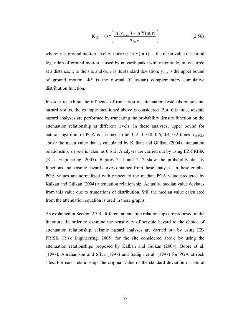
57
⎟⎟⎠
⎞⎜⎜⎝
⎛
σ−
Φ=ΦYln
trun )r,m(Yln)y(ln*K (2.56)
where; y is ground motion level of interest; )r,m(Yln is the mean value of natural
logarithm of ground motion caused by an earthquake with magnitude, m, occurred
at a distance, r, to the site and σln Y is its standard deviation; ytrun is the upper bound
of ground motion, Φ* is the normal (Gaussian) complementary cumulative
distribution function.
In order to exhibit the influence of truncation of attenuation residuals on seismic
hazard results, the example mentioned above is considered. But, this time, seismic
hazard analyses are performed by truncating the probability density function on the
attenuation relationship at different levels. In these analyses, upper bound for
natural logarithm of PGA is assumed to lie 3, 2, 1, 0.8, 0.6, 0.4, 0.2 times σln PGA
above the mean value that is calculated by Kalkan and Gülkan (2004) attenuation
relationship. σln PGA is taken as 0.612. Analyses are carried out by using EZ-FRISK
(Risk Engineering, 2005). Figures 2.11 and 2.12 show the probability density
functions and seismic hazard curves obtained from these analyses. In these graphs,
PGA values are normalized with respect to the median PGA value predicted by
Kalkan and Gülkan (2004) attenuation relationship. Actually, median value deviates
from this value due to truncations of distribution. Still the median value calculated
from the attenuation equation is used in these graphs.
As explained in Section 2.3.4, different attenuation relationships are proposed in the
literature. In order to examine the sensitivity of seismic hazard to the choice of
attenuation relationship, seismic hazard analyses are carried out by using EZ-
FRISK (Risk Engineering, 2005) for the site considered above by using the
attenuation relationships proposed by Kalkan and Gülkan (2004), Boore et al.
(1997), Abrahamson and Silva (1997) and Sadigh et al. (1997) for PGA at rock
sites. For each relationship, the original value of the standard deviation in natural

58
logarithm of PGA as given by the authors is applied. Figure 2.13 shows the hazard
curves obtained from these analyses.
0
0.2
0.4
0.6
0.8
1
1.2
0 1 2 3 4 5 6 7 8 9 10
PGA/Median PGA
Prob
abili
ty D
ensi
ty
untruncatedtruncation at 3 truncation at 2 truncation at 1 truncation at 0.8 truncation at 0.6 truncation at 0.4 truncation at 0.2
σln PGA σln PGA
σln PGA σln PGA σln PGA
σln PGA
σln PGA
Figure 2.11 Probability Density Functions of PGA Truncated at Different Levels
1.00E-06
1.00E-05
1.00E-04
1.00E-03
1.00E-02
1.00E-01
1.00E+00
1.00E+01
0.01 0.1 1 10 100
PGA/Median PGA
Ann
ual P
roba
bilit
y of
Exc
eeda
nce/
Rat
e
UntruncatedTruncated at 0.2 Truncated at 0.4 Truncated at 0.6 Truncated at 0.8 Truncated at 1.0 Truncated at 2.0 Truncated at 3.0
σln PGAσln PGAσln PGAσln PGAσln PGAσln PGAσln PGA
10
1
0.1
0.01
0.001
0.0001
0.00001
0.000001
Figure 2.12 Hazard Curves Corresponding to Truncation of Attenuation Residuals at Different Levels

59
0.00001
0.0001
0.001
0.01
0.1
1
10
0.01 0.1 1 10
PGA(g)
Ann
ual F
requ
ency
of E
xcee
danc
e/R
ate
Kalkan and Gülkan (2004)Abrahamson and Silva (1997)Boore et al. (1997)Sadigh et al. (1997)
Figure 2.13 Hazard Curves Obtained by Using Different Attenuation Relationships It can be observed from Figures 2.10 and 2.13 that seismic hazard results are
sensitive to the choice of attenuation equation as well as to the variability around
the mean prediction equation. Therefore, great care should be paid to determine the
appropriate attenuation equation and the corresponding standard deviation of the
selected ground motion parameter in seismic hazard analysis. Attenuation
relationship should be selected based on the regional tectonic settings of the region
considered. If there is not any reliable local attenuation relationship, equations
developed for the regions with similar tectonic regime can be used. But, the analyst
should check the consistency of these equations and their uncertainties by
comparing them with available ground motion recorded from earthquakes that
occurred at the region considered. In addition, truncation of attenuation residuals
affects the ground motion values estimated especially for very low annual
probabilities of exceedances or very long return periods. This is confirmed by the
hazard curves presented in Figure 2.12. Therefore, the analyst who deals with such
extreme cases should decide on the value of the upper bound of ground motion.

60
2.3.6.2 Uncertainty in the Spatial Distribution of Earthquakes In PSHA, the uncertainty in future earthquake locations is compensated by
delineating line (fault) or area sources.
In the earlier PSHA models, line sources are divided into infinitely small parts and
each part is treated as a point source. Since then, many empirical ground motion
estimation equations which use the shortest distance between the site of interest and
a fault rupture as the distance measure have been developed. In order to use these
relationships in PSHA, the future ruptures of the fault should be estimated. As
explained in Section 2.3.1, there are three different models in literature; namely,
fault-rupture, segmentation and cascading.
In fault-rupture model, estimated rupture length or area is used. In literature, there
are many empirical relationships in which rupture length, RL, is correlated with
earthquake magnitude. They are generally derived based on field observations after
past earthquakes. Table 2.15 summarizes some of these relationships.
It can be seen from Table 2.15 that there is some degree of uncertainty (dispersion)
in rupture length estimated by using the relationships given in the literature. This
uncertainty is incorporated into PSHA computations by considering a set of rupture
lengths for each earthquake magnitude. In other words, rupture of an earthquake
with magnitude, m, is defined to have length, )m(il , given below (Bender and
Perkins, 1987):
[ ] ll ση++= )i(bma)m(Log i10 (2.57)
where a and b are constants; lσ is the standard deviation of rupture length.
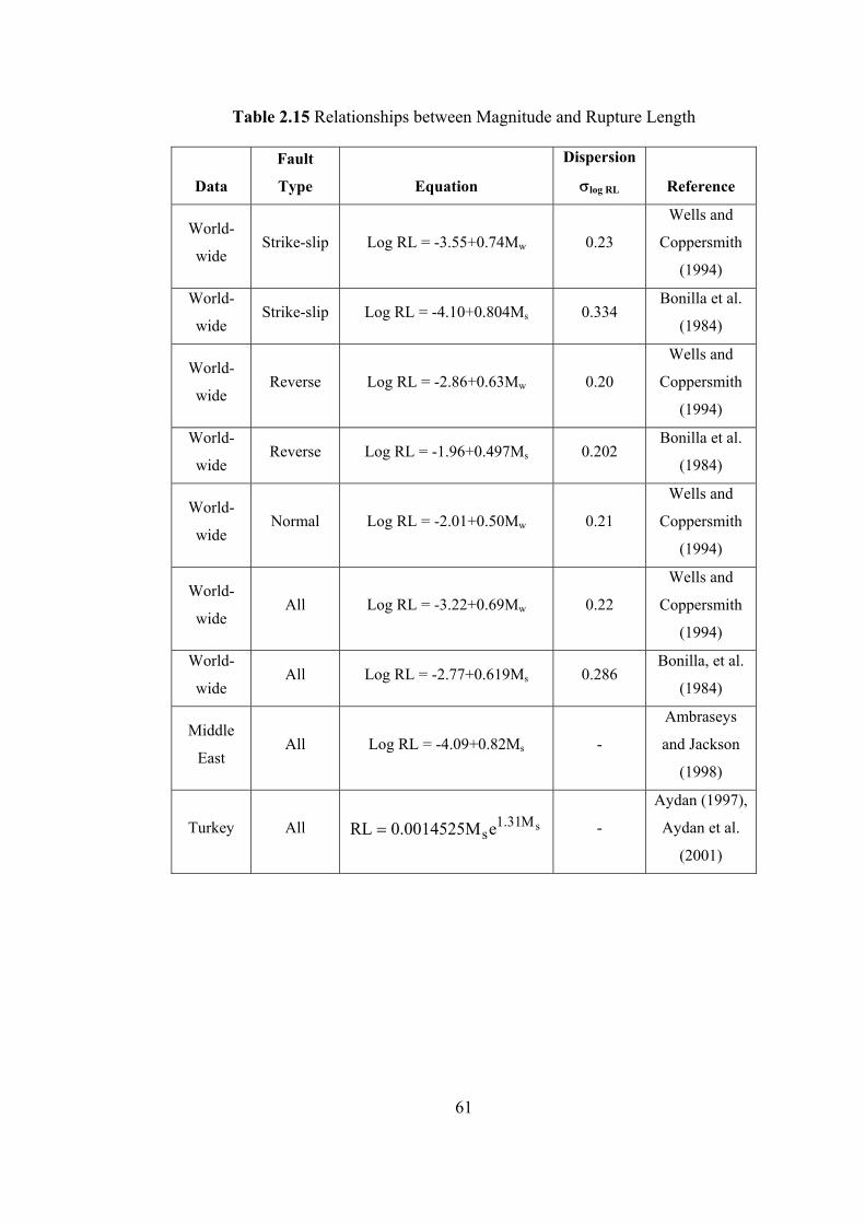
61
Table 2.15 Relationships between Magnitude and Rupture Length
Data
Fault
Type Equation
Dispersion
σlog RL Reference
World-
wide Strike-slip Log RL = -3.55+0.74Mw 0.23
Wells and
Coppersmith
(1994)
World-
wide Strike-slip Log RL = -4.10+0.804Ms 0.334
Bonilla et al.
(1984)
World-
wide Reverse Log RL = -2.86+0.63Mw 0.20
Wells and
Coppersmith
(1994)
World-
wide Reverse Log RL = -1.96+0.497Ms 0.202
Bonilla et al.
(1984)
World-
wide Normal Log RL = -2.01+0.50Mw 0.21
Wells and
Coppersmith
(1994)
World-
wide All Log RL = -3.22+0.69Mw 0.22
Wells and
Coppersmith
(1994)
World-
wide All Log RL = -2.77+0.619Ms 0.286
Bonilla, et al.
(1984)
Middle
East All Log RL = -4.09+0.82Ms -
Ambraseys
and Jackson
(1998)
Turkey All sM31.1seM0014525.0RL = -
Aydan (1997),
Aydan et al.
(2001)

62
The probability of observing the ith rupture length is calculated from (Bender and
Perkins, 1987):
dx2
xexp21)i(p
)1i(f
)i(f
2
∫+
⎟⎟⎠
⎞⎜⎜⎝
⎛−
π= (2.58)
In Eq. (2.58), f(i) is selected in such a way that η(i) is:
f(i) < η(i) ≤ f(i+1)
f(1)= - ∞
f(nr+1)= ∞
∑=
=rn
1i
1)i(p
where nr is the number of possible rupture lengths considered per magnitude.
The rupture in a future earthquake can be located at anywhere along the fault. In
EZ-FRISK (Risk Engineering, 2005), two parameters are used in the determination
of possible rupture locations; namely, horizontal integration increment and vertical
integration increment. The algorithm followed in EZ-FRISK (Risk Engineering,
2005) for the determination of rupture locations is as follows (Dobbs, 2008):
When considering the location of the first rupture, EZ-FRISK first calculates the rupture length. For a given rupture length, the first rupture is placed at 1/2 the rupture length from the start of the fault trace. The last rupture is placed at 1/2 the rupture length from the end of the fault. The number of increments in placing the rupture lengths is calculated by dividing the end position minus the start position by the horizontal integration increment. Then EZ-FRISK calculates the actual horizontal integration increment - this is actually an arc length increment. It proceeds to place the other ruptures at even intervals along the fault. A similar approach is used for the vertical placement.
In order to investigate the effect of rupture length uncertainty on seismic hazard
results, consider the fault discussed in the previous section. It is now assumed that

63
this fault has produced an earthquake with magnitude 6.3. Sites having 1 km, 5 km
and 10 km closest distances to fault are selected as shown in Figure 2.14. Site
names begin with S and continue with closest distance to fault and then relative
location of it from fault like a, b, c…etc. Seismic hazard analyses are performed by
using the rupture length equation developed by Wells and Coppersmith (1994) for
all fault types. The empirical ground motion prediction equation developed by
Kalkan and Gülkan (2004) for peak ground acceleration at rock sites is selected to
model the attenuation characteristics of ground motion. For the standard deviation
of logarithm of rupture length, the value of 0.22 which is given by the Wells and
Coppersmith (1994) is used. In EZ-FRISK (Risk Engineering, 2005), the
uncertainty in rupture length is incorporated into seismic hazard analyses by
defining the number of different discrete ruptures as an input parameter which is
named as number of rupture lengths. Analyses are performed for the sites by
assigning different values to this parameter, i.e. 2, 4, 8, 16 and 100. Also, additional
analyses in which the uncertainty in rupture length is not taken into consideration
are performed by using EZ-FRISK (Risk Engineering, 2005). The difference in
seismic hazard results obtained by ignoring rupture length uncertainty and
considering it by using different numbers of rupture lengths are given in figures
presented in Appendix A.
Figure 2.14 Locations of Fault and Sites Considered in the Analyses Performed to
Investigate the Effect of Rupture Length Uncertainty on Seismic Hazard Results
1 km 5 km
10 km a b c
d e 1 km 5 km
10 km a b c
d e
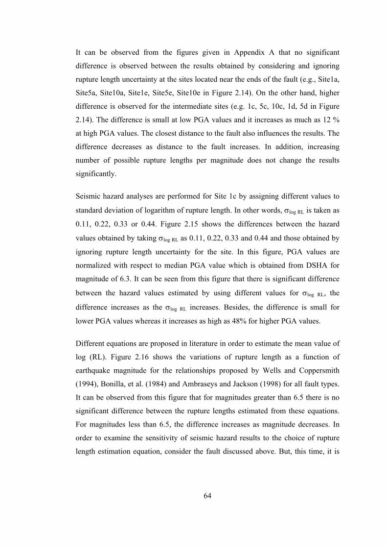
64
It can be observed from the figures given in Appendix A that no significant
difference is observed between the results obtained by considering and ignoring
rupture length uncertainty at the sites located near the ends of the fault (e.g., Site1a,
Site5a, Site10a, Site1e, Site5e, Site10e in Figure 2.14). On the other hand, higher
difference is observed for the intermediate sites (e.g. 1c, 5c, 10c, 1d, 5d in Figure
2.14). The difference is small at low PGA values and it increases as much as 12 %
at high PGA values. The closest distance to the fault also influences the results. The
difference decreases as distance to the fault increases. In addition, increasing
number of possible rupture lengths per magnitude does not change the results
significantly.
Seismic hazard analyses are performed for Site 1c by assigning different values to
standard deviation of logarithm of rupture length. In other words, σlog RL is taken as
0.11, 0.22, 0.33 or 0.44. Figure 2.15 shows the differences between the hazard
values obtained by taking σlog RL as 0.11, 0.22, 0.33 and 0.44 and those obtained by
ignoring rupture length uncertainty for the site. In this figure, PGA values are
normalized with respect to median PGA value which is obtained from DSHA for
magnitude of 6.3. It can be seen from this figure that there is significant difference
between the hazard values estimated by using different values for σlog RL, the
difference increases as the σlog RL increases. Besides, the difference is small for
lower PGA values whereas it increases as high as 48% for higher PGA values.
Different equations are proposed in literature in order to estimate the mean value of
log (RL). Figure 2.16 shows the variations of rupture length as a function of
earthquake magnitude for the relationships proposed by Wells and Coppersmith
(1994), Bonilla, et al. (1984) and Ambraseys and Jackson (1998) for all fault types.
It can be observed from this figure that for magnitudes greater than 6.5 there is no
significant difference between the rupture lengths estimated from these equations.
For magnitudes less than 6.5, the difference increases as magnitude decreases. In
order to examine the sensitivity of seismic hazard results to the choice of rupture
length estimation equation, consider the fault discussed above. But, this time, it is

65
assumed that this fault has produced only earthquakes with magnitude 5.0 in order
to check the sensitivity of results to the rupture length corresponding to smaller
magnitudes. Seismic hazard analyses are carried out for Site 1c by utilizing the
equations developed by Wells and Coppersmith (1994), Bonilla et al. (1984) and
Ambraseys and Jackson (1998) for all fault types. Standard deviation of logarithm
of rupture length is taken as zero in the computations. Figure 2.17 shows the
seismic hazard curves obtained for Site 1c. It can be seen from this figure that there
is no significant difference among the seismic hazard results.
-10
0
10
20
30
40
50
60
70
0 0.5 1 1.5 2 2.5 3
PGA/Median PGA
Diff
eren
ce (%
)
=0.11 =0.22 =0.33 =0.44
σlog RL σlog RL σlog RL σlog RL
Figure 2.15 Differences in Seismic Hazard Values Obtained for Site 1c by Using Different Values of Standard Deviation for Logarithm of Rupture Length
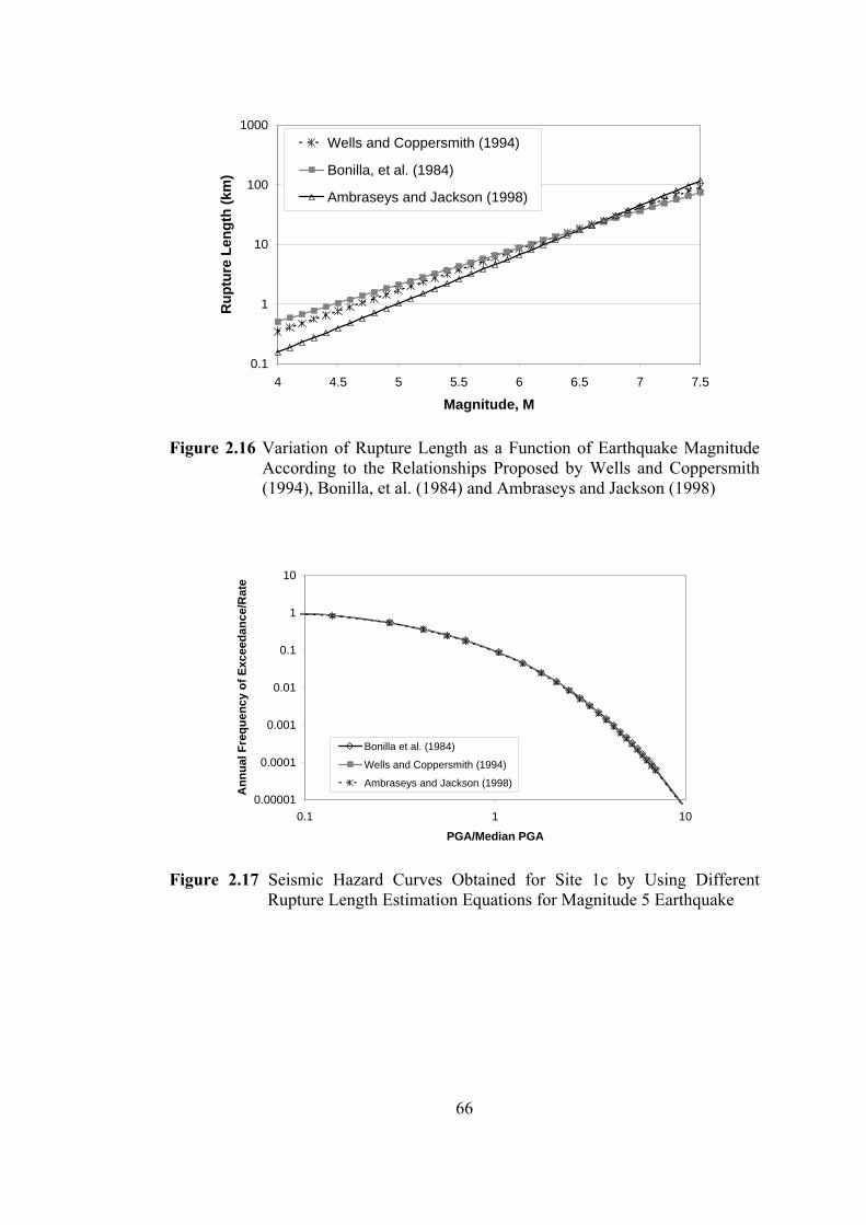
66
0.1
1
10
100
1000
4 4.5 5 5.5 6 6.5 7 7.5
Magnitude, M
Rup
ture
Len
gth
(km
)
Wells and Coppersmith (1994)
Bonilla, et al. (1984)
Ambraseys and Jackson (1998)
Figure 2.16 Variation of Rupture Length as a Function of Earthquake Magnitude According to the Relationships Proposed by Wells and Coppersmith (1994), Bonilla, et al. (1984) and Ambraseys and Jackson (1998)
0.00001
0.0001
0.001
0.01
0.1
1
10
0.1 1 10
PGA/Median PGA
Ann
ual F
requ
ency
of E
xcee
danc
e/R
ate
Bonilla et al. (1984)
Wells and Coppersmith (1994)
Ambraseys and Jackson (1998)
Figure 2.17 Seismic Hazard Curves Obtained for Site 1c by Using Different Rupture Length Estimation Equations for Magnitude 5 Earthquake
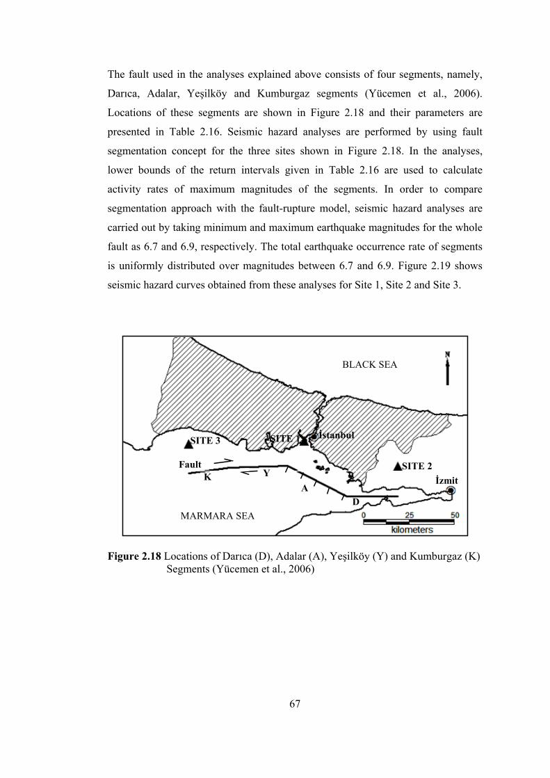
67
The fault used in the analyses explained above consists of four segments, namely,
Darıca, Adalar, Yeşilköy and Kumburgaz segments (Yücemen et al., 2006).
Locations of these segments are shown in Figure 2.18 and their parameters are
presented in Table 2.16. Seismic hazard analyses are performed by using fault
segmentation concept for the three sites shown in Figure 2.18. In the analyses,
lower bounds of the return intervals given in Table 2.16 are used to calculate
activity rates of maximum magnitudes of the segments. In order to compare
segmentation approach with the fault-rupture model, seismic hazard analyses are
carried out by taking minimum and maximum earthquake magnitudes for the whole
fault as 6.7 and 6.9, respectively. The total earthquake occurrence rate of segments
is uniformly distributed over magnitudes between 6.7 and 6.9. Figure 2.19 shows
seismic hazard curves obtained from these analyses for Site 1, Site 2 and Site 3.
BLACK SEA
MARMARA SEA
İstanbul
İzmitK YA
D
Fault SITE 2
SITE 1SITE 3
Figure 2.18 Locations of Darıca (D), Adalar (A), Yeşilköy (Y) and Kumburgaz (K) Segments (Yücemen et al., 2006)

68
Table 2.16 Parameters of the Darıca, Adalar, Yeşilköy and Kumburgaz Segments
Segment Name Type Length
(km) Maximum Magnitude
Recurrence Interval* (RI)
(in years)
Darıca Strike Slip 28 6.8 500 < RI ≤ 1000
Adalar Normal 37 6.9 200 < RI ≤ 500
Yeşilköy Strike Slip 31 6.8 257±23
Kumburgaz Strike Slip 23 6.7 257±23
* Recurrence intervals of the segments are taken from Yücemen et al. (2006). It can be observed from Figure 2.19 that segmentation and fault-rupture models
may give different seismic hazard results depending on the earthquake occurrence
rate of the segment nearest to the site as well as its maximum magnitude. Since
earthquake magnitudes and their occurrence rates are distributed over the whole
fault in the fault-rupture model, seismic hazard values predicted by using this model
are higher at the sites which are located near the segment with low earthquake
magnitude and earthquake occurrence rate. In this example, there is no significant
difference between maximum magnitudes of the segments. Therefore, the
difference may result from the earthquake occurrence rates of the segments. In Site
1 and Site 2, no significant difference is observed between the results obtained by
using these two models. On the other hand, in Site 3 where Kumburgaz segment is
the most critical source of seismic threat and its earthquake occurrence rate is high,
segmentation model gives higher seismic hazard results compared with fault-
rupture model. It should be noted that the difference between these two models is
expected to increase as distance to fault decreases. As a result, the analyst should
make detailed investigations to determine boundaries, maximum magnitudes and
earthquake occurrence rates of the segments of a fault or fault system to apply the
fault segmentation model in seismic hazard analysis.

69
0.00001
0.0001
0.001
0.01
0.1
0.01 0.1 1 10
PGA (g)
Ann
ual F
requ
ency
of E
xcee
danc
e
Segmentation Model
Fault Rupture Model
(a) Site1
0.00001
0.0001
0.001
0.01
0.1
0.01 0.1 1 10PGA (g)
Ann
ual F
requ
ency
of E
xcee
danc
e Segmentation Model
Fault Rupture Model
(b) Site2
0.00001
0.0001
0.001
0.01
0.1
0.01 0.1 1 10PGA (g)
Ann
ual F
requ
ency
of E
xcee
danc
e Segmentation Model
Fault Rupture Model
(c) Site3
Figure 2.19 Seismic Hazard Curves Obtained by Considering Segmentation
Concept and Fault-Rupture Model

70
For the segments explained above, the cascading methodology developed by
Cramer et al. (2000) is also applied. In literature, this methodology is generally
applied to rupture probabilities of segments calculated by using time dependent or
renewal models. In order to compare the seismic hazard results obtained from the
cascade model with those from the fault segmentation model, the probability of
earthquake occurrences in 50 years is calculated for each segment based on the
Poisson model. Table 2.17 shows the calculations carried out to obtain multi-
segment and individual segment rupture probabilities by using the Eqs. (2.2) and
(2.3) given in Section 2.3.1. The probabilities, Pcj, given in the final stage are
converted to equivalent Poisson rates by using the equation given below;
w
)P1ln( cjeq
−−=ν (2.59)
Figure 2.20 shows seismic hazard curves obtained for the sites shown in Figure 2.18
by using the cascade and fault segmentation models.
Compared with segmentation model, cascade model gives higher seismic hazard
values for high PGA values whereas it resulted in lower values for low PGA values.
This result is expected due to the reason that cascading of contiguous segments into
longer ruptures results in an increase in maximum magnitude. Since cascade model
is based on conservation of seismic moment rate, the total rate of earthquakes
decreases as maximum magnitude of multi-segment rupture rises.
Sometimes, geographic conditions are the constraints to determine the exact
locations of faults. This is the case for the segments discussed above because they
extend beneath the Marmara Sea. Therefore, their locations are determined by
bathymetry and reflection survey. In addition, there is an uncertainty in the
locations of past earthquakes. Therefore, the epicenter of an earthquake generated
by a fault may be located away from it due to prediction errors. In such a case, the
narrow area sources can be used to compensate for these uncertainties.

71
Table 2.17 Calculations of Multi-Segment and Individual Segment Probabilities According to the Cascade Methodology Defined by Cramer et al. (2000)
Cascade or Segment
Length (km)
Mmax
Pi
1-(1-Psi)/∏(1-Pcj)
Pcj
1 D+A+Y+K 119 7.5 - 0.095163 Darıca (D) 28 6.8 0.095163 1-(1-0.095163)/(1-0.095163)* 0 Adalar (A) 37 6.9 0.221199 1-(1-0.221199)/(1-0.095163)= 0.139291
Yeşilköy (Y) 31 6.8 0.192389 1-(1-0.192389)/(1-0.095163)= 0.107451 Kumburgaz (K) 23 6.7 0.192389 1-(1-0.192389)/(1-0.095163)= 0.107451
2
A+Y+K 91 7.4 - 0.107451 Adalar (A) 37 6.9 0.139291 1-(1-0.139291)/(1-0.107451)= 0.035673
Yeşilköy (Y) 31 6.8 0.107451 1-(1-0.107451)/(1-0.107451)* 0 Kumburgaz (K) 23 6.7 0.107451 1-(1-0.107451)/(1-0.107451)* 0
Final
D+A+Y+K 119 7.5 - 0.095163
A+Y+K 91 7.4 - 0.107451
Darıca (D) 28 6.8 0.095163 1-(1-0.095163)/(1-0.095163)* 0
Adalar (A) 37 6.9 0.221199 1-(1-0.221199)/(1-0.095163) /(1-0.107451)= 0.035673
Yeşilköy (Y) 31 6.8 0.192389 1-(1-0.192389)/(1-0.095163) /(1-0.107451)= 0
Kumburgaz (K) 23 6.7 0.192389 1-(1-0.192389)/(1-0.095163) /(1-0.107451)= 0
* Although Pcj values for the segments with Pi values equal to cascade probability are equal to zero, Eq. (2.3) gives meaningless Pcj values.

72
0.000001
0.00001
0.0001
0.001
0.01
0.1
0.01 0.1 1 10PGA (g)
Ann
ual F
requ
ency
of E
xcee
danc
e Segmentation Model
Cascade Model
(a) Site1
0.000001
0.00001
0.0001
0.001
0.01
0.1
0.01 0.1 1 10PGA (g)
Ann
ual F
requ
ency
of E
xcee
danc
e Segmentation Model
Cascade Model
(b) Site 2
0.00001
0.0001
0.001
0.01
0.1
0.01 0.1 1 10PGA (g)
Ann
ual F
requ
ency
of E
xcee
danc
e
Segmentation Model
Cascade Model
(c) Site 3
Figure 2.20 Seismic Hazard Curves Obtained for the Three Sites by Using Cascade
and Fault Segmentation Models
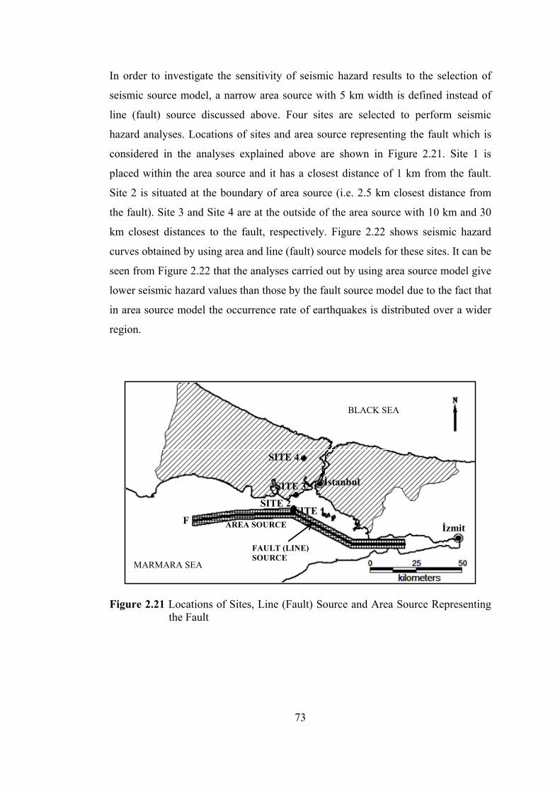
73
In order to investigate the sensitivity of seismic hazard results to the selection of
seismic source model, a narrow area source with 5 km width is defined instead of
line (fault) source discussed above. Four sites are selected to perform seismic
hazard analyses. Locations of sites and area source representing the fault which is
considered in the analyses explained above are shown in Figure 2.21. Site 1 is
placed within the area source and it has a closest distance of 1 km from the fault.
Site 2 is situated at the boundary of area source (i.e. 2.5 km closest distance from
the fault). Site 3 and Site 4 are at the outside of the area source with 10 km and 30
km closest distances to the fault, respectively. Figure 2.22 shows seismic hazard
curves obtained by using area and line (fault) source models for these sites. It can be
seen from Figure 2.22 that the analyses carried out by using area source model give
lower seismic hazard values than those by the fault source model due to the fact that
in area source model the occurrence rate of earthquakes is distributed over a wider
region.
BLACK SEA
MARMARA SEA
İstanbul
İzmitF
SITE 2
SITE 3
SITE 1
SITE 4
FAULT (LINE) SOURCE
AREA SOURCE
Figure 2.21 Locations of Sites, Line (Fault) Source and Area Source Representing the Fault
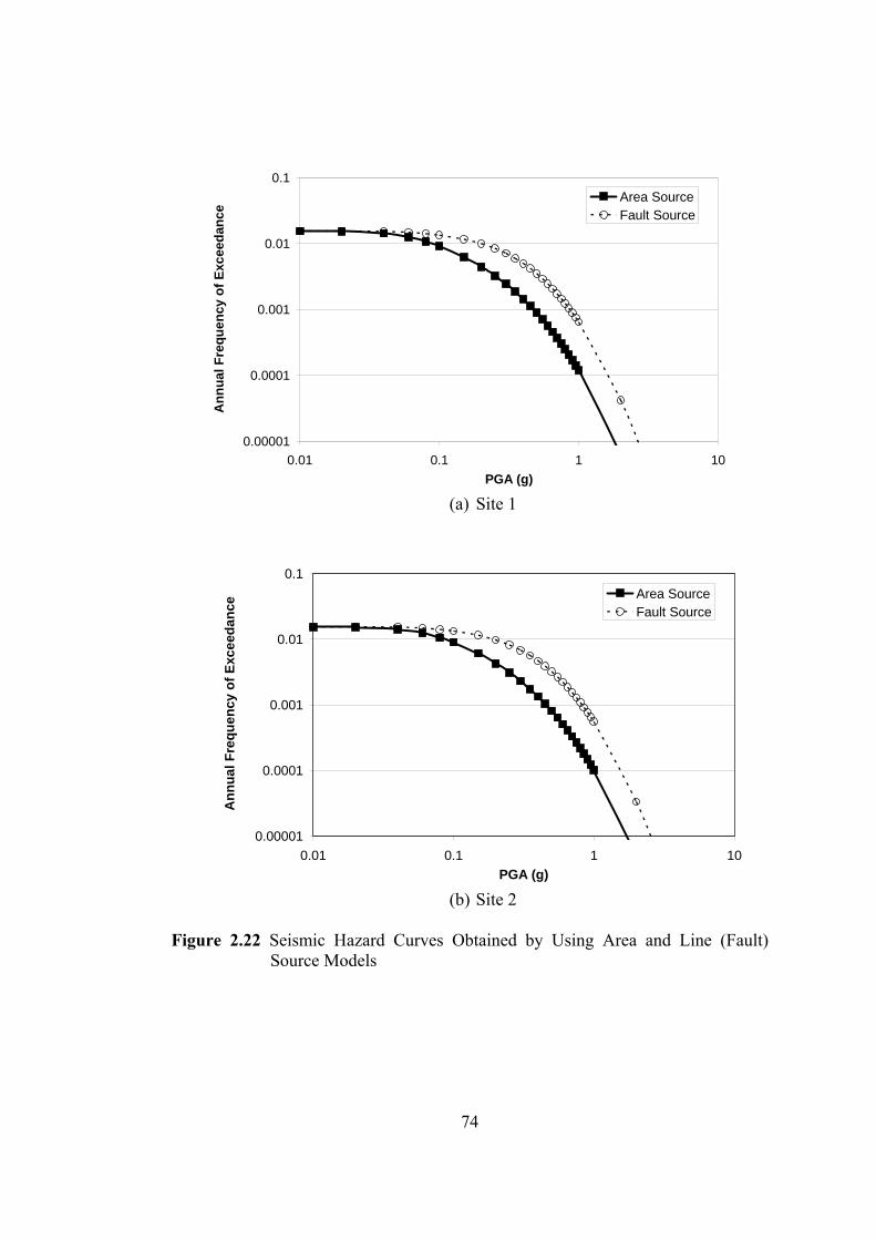
74
0.00001
0.0001
0.001
0.01
0.1
0.01 0.1 1 10PGA (g)
Ann
ual F
requ
ency
of E
xcee
danc
eArea SourceFault Source
(a) Site 1
0.00001
0.0001
0.001
0.01
0.1
0.01 0.1 1 10PGA (g)
Ann
ual F
requ
ency
of E
xcee
danc
e Area SourceFault Source
(b) Site 2
Figure 2.22 Seismic Hazard Curves Obtained by Using Area and Line (Fault)
Source Models

75
0.00001
0.0001
0.001
0.01
0.1
0.01 0.1 1 10PGA (g)
Ann
ual F
requ
ency
of E
xcee
danc
e
Area SourceFault Source
(c) Site 3
0.00001
0.0001
0.001
0.01
0.1
0.01 0.1 1 10PGA (g)
Ann
ual F
requ
ency
of E
xcee
danc
e
Area SourceFault Source
(d) Site 4
Figure 2.22 (Continued) Seismic Hazard Curves Obtained by Using Area and Line
(Fault) Source Models

76
It can be observed from the results of the analyses explained in this section that
seismic hazard results are sensitive to source modeling (area or line). In literature,
different methods; i.e. fault-rupture, segmentation and cascade models, are
proposed for computation of seismic hazard from faults. In order to implement
segmentation and cascade models, more detailed information (i.e., boundaries of
segments, cascade scenarios, etc.) is required. Therefore, the analyst should select
the source model depending on the level of available information. If the location of
the fault has uncertainties, the area source model can be preferred instead of the line
model. For faults whose segments are examined in detail, fault segmentation model
can be used instead of the fault-rupture model. On the other hand, the rupture
histories of the fault or other investigations are required to decide on the probable
multi-segment rupture scenarios in the cascade model.
The delineation of area sources may involve uncertainity. One of the alternatives to
include this uncertainity into the seismic hazard analysis is to assume randomness in
the location of the boundaries of seismic sources (Bender, 1986; Yücemen and
Gülkan, 1994). According to this assumption, the introduction of the seismic source
zone boundary uncertainity causes the seismicity concentrated around a seismic
source to be dispersed over a wider region proportional to the standard deviation
modeling this uncertainity. This causes a decrease in the intensity of seismic hazard
in the neighbourhood of the seismic source, since the seismicity is distributed over a
larger area. Based on a study conducted for Jordan, Yücemen (1995) concluded that
for sites under the threat of a number of seismic sources of either type (i.e. area or
line), the incorporation of source location uncertainty influences the hazard estimate
to a relatively smaller extent compared to other factors of uncertainty, such as the
uncertainty involved in the attenuation model.

77
2.3.6.3 Uncertainty in the Magnitude Distribution
Uncertainty in the magnitude of a future earthquake that will occur in a seismic
source is incorporated into PSHA by defining an appropriate magnitude recurrence
relationship. The widely used models in seismic hazard studies are the truncated
exponential distribution, characteristic earthquake model developed by Youngs and
Coppersmith (1985) and maximum magnitude model.
Consider again the same fault and Site 1, Site 3 and Site 4 shown in Figure 2.21 and
assume that the lower and upper bounds for the earthquake magnitudes are 4.5 and
7.5, respectively. The slope of the exponential magnitude distribution, |β|, is taken
as 1.23 and the annual mean rate for earthquakes with m ≥ 4.5, ν, is assumed as 0.2.
Seismic hazard analyses are performed by using truncated exponential distribution
(TED) and characteristic earthquake model (CEM) developed by Youngs and
Coppersmith (1985). In order to model the attenuation characteristics of ground
motions, the empirical equation proposed by Kalkan and Gülkan (2004) for PGA at
rock sites is used. A value of 0.612 is assigned to the standard deviation in natural
logarithm of PGA. Figure 2.23 shows probability density functions corresponding
to TED and CEM with varying Δm values, where Δm is the magnitude width
between the lower bound of the characteristic earthquake magnitudes and the
exponentially distributed magnitude whose probability density is assumed to be
equal to probability densities of characteristic earthquakes and it is shown as a
sketch in Figure 2.23.
Seismic hazard analyses are carried out also by using the maximum magnitude or
purely characteristic earthquake model (PCEM). First, the rate associated with the
characteristic earthquakes and which is uniformly distributed over the interval (m1,
m1–0.5) in the CEM with Δm=1.0, is now lumped completely onto the maximum
magnitude, m1, (PCEM) and the remaining rate is assigned to the range of the
exponentially distributed magnitudes (4.5≤m≤7.0). Then, a truncated Gaussian
distribution (TGD) is used to consider uncertainty in the maximum magnitude. The

78
mean value of maximum magnitude, μm, is taken as 7.5 and its standard deviation,
σm, as 0.28 as given by Wells and Coppersmith (1994) for the equation which
relates magnitude with rupture length. The lower and upper limits of the distribution
are assumed as μm-σm and μm+σm and the rate of characteristic earthquakes
calculated by using CEM with Δm=1.0 is distributed on the magnitudes between
this range. To account for other earthquakes with smaller magnitudes, remaining
rate is assigned to the range of the exponentially distributed magnitudes
(4.5≤m≤7.0). Figure 2.24 shows probability density functions corresponding to
these models.
0.00
0.20
0.40
0.60
0.80
1.00
1.20
1.40
1.60
4 4.5 5 5.5 6 6.5 7 7.5 8
Magnitude,m
f M(m
)
Figure 2.23 Probability Density Functions Corresponding to Truncated Exponential
Distribution (TED) and Characteristic Earthquake Model (CEM) with Varying Δm values
Seismic hazard analyses are carried out by using EZ-FRISK (Risk Engineering,
2005). Figure 2.25 shows the seismic hazard curves for Site 4 estimated by using
the magnitude distributions presented in Figures 2.23 and 2.24. Since general trends
CEM-Δm=2.5
CEM-Δm=2.0
TED CEM-Δm=0
CEM-Δm=1.5 CEM-Δm=1.0 CEM-Δm=0.5
Δm
Magnitude, m
f M(m
)
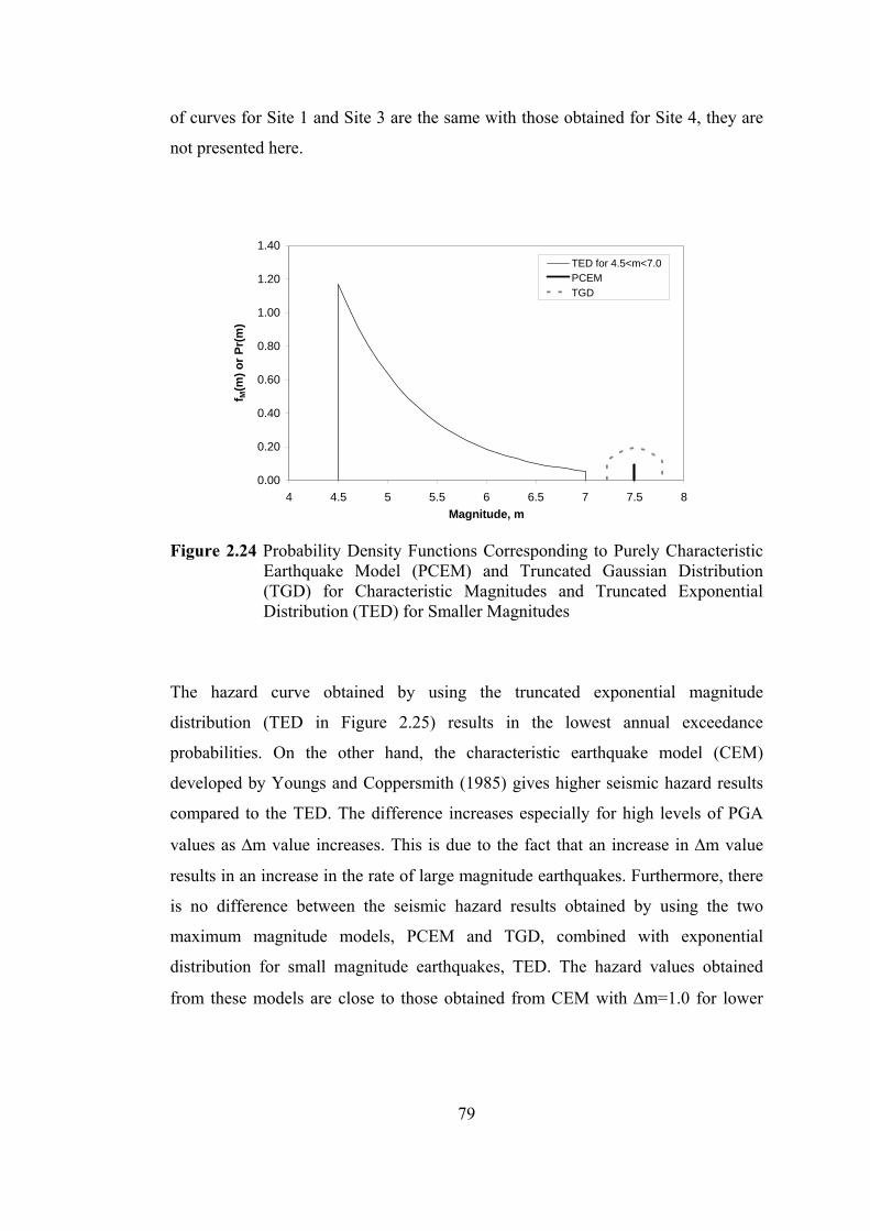
79
of curves for Site 1 and Site 3 are the same with those obtained for Site 4, they are
not presented here.
0.00
0.20
0.40
0.60
0.80
1.00
1.20
1.40
4 4.5 5 5.5 6 6.5 7 7.5 8Magnitude, m
f M(m
) or P
r(m
)
TED for 4.5<m<7.0PCEMTGD
Figure 2.24 Probability Density Functions Corresponding to Purely Characteristic Earthquake Model (PCEM) and Truncated Gaussian Distribution (TGD) for Characteristic Magnitudes and Truncated Exponential Distribution (TED) for Smaller Magnitudes
The hazard curve obtained by using the truncated exponential magnitude
distribution (TED in Figure 2.25) results in the lowest annual exceedance
probabilities. On the other hand, the characteristic earthquake model (CEM)
developed by Youngs and Coppersmith (1985) gives higher seismic hazard results
compared to the TED. The difference increases especially for high levels of PGA
values as Δm value increases. This is due to the fact that an increase in Δm value
results in an increase in the rate of large magnitude earthquakes. Furthermore, there
is no difference between the seismic hazard results obtained by using the two
maximum magnitude models, PCEM and TGD, combined with exponential
distribution for small magnitude earthquakes, TED. The hazard values obtained
from these models are close to those obtained from CEM with Δm=1.0 for lower

80
PGA values whereas these models yield almost same results with CEM with
Δm=1.5 for higher PGA values.
1.00E-05
1.00E-04
1.00E-03
1.00E-02
1.00E-01
1.00E+00
0.01 0.1 1 10
PGA(g)
Ann
ual F
requ
ency
of E
xcee
danc
e
TED CEM-Δm=0 CEM-Δm=0.5 CEM-Δm=1.0 CEM-Δm=1.5 CEM-Δm=2.0 CEM-Δm=2.5 PCEM&TED TGD&TED
0.00001
0.0001
0.001
0.01
0.1
1
Figure 2.25 Seismic Hazard Curves for Site 4 Corresponding to: Truncated
Exponential Distributions for 4.5<m<7.5 (TED); Characteristic Earthquake Model (CEM) with Varying Δm values; Purely Characteristic Earthquake Model Combined with Exponential Distribution for Smaller Magnitudes (4.5≤m≤7.0) (PCEM&TED); Truncated Gaussian Distribution for Characteristic Magnitudes (7.22≤m≤7.78) Combined with Exponential Distribution for Smaller magnitudes (4.5≤m≤7.0) (TGD&TED)
2.3.6.4 Uncertainty in the Temporal Distribution of Earthquakes In PSHA, two stochastic models, namely Poisson and renewal, are generally applied
to predict probability of future earthquake occurrences. Seismic hazard analyses
presented in the previous section are all based on the Poisson model. In this section,
additional analyses are performed by using the renewal model in order to
investigate the sensitivity of seismic hazard results to the choice of earthquake
occurrence models in time domain.
81
Consider the fault described in the previous section. In the renewal model,
probability distribution of inter-event times of characteristic earthquakes and time
elapsed since the last event are used to predict probabilities of the occurrence of
future earthquakes. Based on the characteristic earthquake rate obtained from the
characteristic earthquake model with Δm=1.0, mean inter-event time of the
earthquakes on this fault is estimated as 54 years. In order to determine the date of
the last characteristic earthquake, the recent study of Parsons (2004) in which the
ruptures resulted from historical earthquakes have been estimated as shown in
Figure 2.26 is used. It can be observed from Figure 2.26 that after 1509 M∼7.4
earthquake that is estimated to rupture the whole length of the fault, May 1766
M∼7.2 earthquake ruptured a large part of it. Therefore, it can be assumed that May
1766 event released almost all of the energy accumulated and it is the last
characteristic earthquake occurred on this fault. Thus, time elapsed since this event
is 241 years.
Brownian Passage Time (BPT) and lognormal (LN) distributions are selected as the
probability distribution functions for the inter-event times. Aperiodicity used in
BPT distribution is assumed to be 0.5, which appears to be the most likely value
according to the study conducted by Ellsworth et al. (1999). Since coefficient of
variation equals to aperiodicity, it is also assumed to be 0.5. Figures 2.27 and 2.28
show probability density and hazard functions obtained for the BPT and LN
distributions, respectively. As observed from these figures there is no significant
difference between the functions derived from these two distributions.

82
NN
N N
NN
N N
Figure 2.26 Estimated Ruptures (Thick Dashed Green Lines), Modified Mercalli Intensity (MMI) Values (Yellow Dots), Sites of Damage Potentially Enhanced by Soft Sediments (Red Dots), Moment Magnitude M Needed to Satisfy the Observations for a Given Location (Red Dashed Contours) for Large Earthquakes Occurred between A.D. 1500 and 2000 (After Parsons, 2004).

83
0.0000
0.0050
0.0100
0.0150
0.0200
0.0250
0 50 100 150 200Time Elapsed Since the Last Characteristic Earthquake
(year)
Prob
abili
ty D
ensi
ty
Brownian Passage Time ModelLognormal Distribution
Figure 2.27 Probability Density Functions Corresponding to the BPT and LN Distributions Based on the Mean Inter-Event Time of µT =54 years and α=cov=0.5
0.0000.0050.0100.0150.0200.0250.0300.0350.0400.0450.050
0 50 100 150 200Time Elapsed Since the Last Characteristic Earthquake
(year)
Haz
ard
Rat
e
Brownian Passage Time Model
Lognormal Distribution
Figure 2.28 Hazard Functions Corresponding to the BPT and LN Distributions Based on the Mean Inter-Event Time of µT =54 years and α=cov=0.5
84
In the renewal hybrid model, the mean rate of characteristic earthquakes depends on
probability distribution function of inter-event times as well as the time elapsed
since the last characteristic earthquake, “t0”, and the next time interval, “w”.
Besides, depending on the information available for t0, either Eq. (2.20) (if t0 is
known) or Eq. (2.28) (if t0 is unknown) will be combined with Eq. (2.25) to
calculate the mean rate of characteristic earthquakes. In this study, “w” is assumed
to be 50 years. Two cases are considered. In the first case t0 is set equal to an
arbitrary value of t years and in the second case it is assumed to be greater than t
years. Mean rates of characteristic earthquakes are calculated for these two cases by
using BPT and LN distributions and are shown in Figure 2.29 for t/µT values
changing between 0 and 3. Again no significant difference is observed between the
general trends of these two distributions. Accordingly the BPT distribution is
adopted to describe the inter-event times of the characteristic earthquakes in the
renewal model.
Together with the renewal model both characteristic (Youngs and Coppersmith,
1985) and pure characteristic (maximum magnitude) models are utilized as the
magnitude-recurrence relationships. Mean rate of characteristic earthquakes is
calculated for t0=241 years. Note that there is no significant difference between
mean rates of characteristic earthquakes for t0=241 years and t0≥241 years. Mean
rate of characteristic earthquakes is assumed either uniformly distributed over
magnitudes between m1 and m1 – 0.5 (CEM) or assigned only to m1 (PCEM). The
rate of smaller magnitude earthquakes (4.5≤m≤7.0) is obtained by subtracting the
equivalent mean rate of characteristic earthquakes from the annual mean rate ν for
earthquakes with m ≥ 4.5. Figure 2.30 shows seismic hazard curves obtained for
Site 4 considered in the previous section from the renewal model combined with
CEM and PCEM. In this figure, seismic hazard curves shown in Figure 2.25 for the
CEM with Δm=1.0 and PCEM&TED are also presented in order to compare the
results with those obtained from the Poisson model.

85
0.000
0.005
0.010
0.015
0.020
0.025
0.030
0.035
0.040
0.045
0 0.5 1 1.5 2 2.5 3t/μT
Equ
ival
ent M
ean
Rat
e of
Cha
ract
eris
tic
Ear
thqu
akes
t >tt =t0 0
(a) BPT Distribution
0.000
0.005
0.010
0.015
0.020
0.025
0.030
0.035
0.040
0.045
0 0.5 1 1.5 2 2.5 3t/μT
Equ
ival
ent M
ean
Rat
e of
Cha
ract
eris
tic
Ear
thqu
akes t >t
t =t0 0
(b) Lognormal Distribution
Figure 2.29 Variation of Equivalent Mean Rate of Characteristic Earthquakes
Calculated Based on Eqs. (2.20) and (2.28) for the BPT and LN Distributions

86
Figure 2.30 Seismic Hazard Curves for Site 4 Corresponding to the Combinations of Renewal Model with PCEM&TED and CEM; Poisson Model with PCEM and CEM with Δm=1.0
It can be observed from Figure 2.30 that renewal model gives consistently higher
seismic hazard results compared to the Poisson assumption. In this example,
compared with the mean inter-event time, a considerably long time (more than four
times mean inter-event time) has passed after the last characteristic event. Thus, the
rate of characteristic earthquake occurrence and consequently its probability
increased in the renewal model. It can be seen from Figure 2.29 that immediately
after the occurrence of the characteristic earthquake, this probability decreases. In
such a case, the seismic hazard results are expected to be lower compared with
those of the Poisson model. Therefore, the analyst should be careful in the
determination of the values to be assigned to the parameters used in the renewal
model. In this study, BPT model with aperiodicity of 0.5 is selected as inter-event
time distribution. It can be observed from Figure 2.29 (a) that the rates calculated
for the cases in which t0 is known or unknown are almost the same when t0 is
greater than 1.5 times of the mean inter-event time, μT. Therefore, in this case study,
there is no need to spend an extra effort in the evaluation of t0 value if it is expected
0.00001
0.0001
0.001
0.01
0.1
1
0.01 0.1 1 10
PGA(g)
Ann
ual F
requ
ency
of E
xcee
danc
e Renewal with CEM
Renewal with PCEM&TED
Poisson with CEM- =1.0
Poisson with PCEM&TED
Δm

87
to be greater than 1.5 times of the μΤ value. In addition, the same trend is observed
for the Poisson model with respect to the recurrence models: i.e. the PCEM&TED
giving higher seismic hazard values compared to those of CEM.
2.3.6.5 Uncertainties in Earthquake Catalogs Earthquake catalogs are the most important sources of information used in seismic
hazard analysis since they describe the spatial and temporal distribution of past
earthquakes in the interested region. Unfortunately, certain degree of uncertainty
results from the earthquake catalogs. Generally, earthquake magnitudes are reported
in different magnitude scales in these catalogs and it is desirable to convert them
into a common one. The other problem is that earthquake catalogs are generally
incomplete for small magnitude earthquakes occurred in the ancient times due to
inadequate instrumentation spread or scatter of relatively small population before
the period of complete recording (Deniz, 2006).
The incompleteness of earthquake catalog creates biases in the database both in
time and space. Accordingly, the resulting recurrence relationships may not
represent the true long term rates. In other words, the annual rate of occurrences of
smaller magnitude earthquakes and the absolute value of the slope of the recurrence
relation are underestimated from the incomplete databases. For this reason, it is
necessary to determine the time period over which the data in a given magnitude
interval is completely reported. After the determination of complete time interval,
the annual rate of earthquake occurrences having that magnitude range is computed
by considering only that time interval.
2.3.7 Logic Tree Methodology As explained in the previous section, different seismic hazard curves can be
obtained by using different models and input parameters. The simple and systematic
way to aggregate the epistemic uncertainities is to utilize the logic tree method.
88
A general logic tree model (Risk Engineering, 2006) is shown in Figure 2.31. A
logic tree consists of nodes and branches. Each node represents a model, an input
parameter, or an assumption that is uncertain. Branches extending from each node
are discrete alternatives for that model, input parameter, or assumption. The nodes
should be ordered in such a way that independent nodes are placed to the left while
dependent ones are located to the right. The end branches of the logic tree represent
mutually exclusive and collectively exhaustive states of all uncertain parameters,
models and assumptions. Seismic hazard analysis is carried out for each end branch.
For each seismic hazard curve, a subjective weight (discrete probability) which is
equal to the product of weights on the branches leading to its corresponding end
branch is assigned. Seismic hazard results are aggregated by using the theorem of
total probability, which can be expressed through the following relationship
(Yücemen, 1982):
( ) ( ) in
1ii wGyYPyYP ∑
=>=> (2.60)
where, Gi = combination of uncertain parameters, models or assumptions at the ith
end branch; wi = P(Gi), subjective joint probability assigned to the ith end branch
reflecting its likelihood to be “true” compared to the others; n = number of end
branches. It is to be noted that the sum of wi’s will be equal to unity. The seismic
hazard obtained in this way is generally called as the Bayesian estimate.
The use of logic trees in probabilistic seismic hazard analysis often involves a large
number of branches that reflect the uncertainty in the selection of different models
and input parameters assigned to each model. It requires a long computation time
due to several branches that might sometimes be unnecessary due to their little or no
influence on the results. Therefore the sensitivity analysis is useful to discriminate
which parameters contribute the most to the seismic hazard and its uncertainty, and
can be used as a preliminary step for the construction of logic trees focusing efforts
on the parameters found to be most sensitive (Barani et al., 2007).

89
Figure 2.31 A General Logic Tree (After Risk Engineering, 2006)
a1 Pr(a1)
c1 Pr(c1/a1∩b2)
c2 Pr(c2/a1∩b2)
c3 Pr(c3/a1∩b2)
b2 Pr(b2/a1)
b1 Pr(b1/a1)
c1 Pr(c1/a1∩b1)
c2 Pr(c2/a1∩b1)
c3 Pr(c3/a1∩b1)
b3 Pr(b3/a2)
b1 Pr(b1/a2)
a2 Pr(a2)
b2 Pr(b2/a2)
c1 Pr(c1/a2∩b1)
c3 Pr(c3/a2∩b1)
c1 Pr(c1/a2∩b2)
c1 Pr(c1/a2∩b3)
c2 Pr(c2/a2∩b3)
c3 Pr(c3/a2∩b3)
h(a1.b1.c1) Pr(a1∩b1∩c1)
h(a1.b1.c2) Pr(a1∩b1∩c2)
h(a1.b1.c3) Pr(a1∩b1∩c3)
h(a1.b2.c1) Pr(a1∩b2∩c1)
h(a1.b2.c2) Pr(a1∩b2∩c2)
h(a1.b2.c3) Pr(a1∩b2∩c3)
h(a2.b1.c1) Pr(a2∩b1∩c1)
h(a2.b1.c3) Pr(a2∩b1∩c3)
h(a2.b2.c1) Pr(a2∩b2∩c1)
h(a2.b3.c1) Pr(a2∩b3∩c1)
h(a2.b3.c2) Pr(a2∩b3∩c2)
h(a2.b3.c3) Pr(a2∩b3∩c3)
PARAMETER or
MODEL, A
PARAMETER or
MODEL, B
PARAMETER or
MODEL, C
DISTRIBUTION of H(A,B,C)
Note that Pr(ai∩bj∩ck)= Pr(ck/ai∩bj). Pr(bj/ai). Pr(ai)

90
The other important point in logic tree methodology is the relative weight assigned
to each branch of the logic tree. Final result depends on the subjective probabilities
assigned to different alternatives as well as the alternatives taking place in the logic
tree. Therefore, extreme care should be paid to the process of assigning these
probabilities. Sabetta et al. (2005) carried out an investigation on sensitivity of
probabilistic seismic hazard analyses results to ground motion relations and logic
tree weights. The results obtained from their study showed that when four or more
ground motion prediction relationships are included, the relative weigths assigned
to these relationships do not significantly influence the hazard unless strongly
biased towards one or two relations. They stated that the choice of appropriate
relationships to be included in the analysis has a greater impact than the weigths
assigned to these relationships.
2.3.8 Deaggregation of Seismic Hazard The probabilistic seismic hazard results can be disaggregated to determine the
contribution of the magnitudes, distances and epsilon values to the calculated
exceedance probabilities. The epsilon is the number of standard deviations that the
ground motion value deviates from the median ground motion value for an event
defined by the mean magnitude and distance. In other words, it is equal to
y/)yy( σ− , where y is the logarithm of ground motion value to be deaggregated, y
and σy are the mean value and standard deviation of the logarithm of ground
motion, respectively. The procedure that examines the spatial, magnitude and
epsilon dependence of hazard results is called disaggregation or deaggregation.
In this procedure, the magnitude, distance and epsilon values are divided into bins.
In order to calculate the relative contribution of each bin to the total exceedance
probability of a specified ground motion value, the exceedance probability due to
each bin is calculated and divided by the total exceedance probability of all bins.
Results of this process can be presented as histograms that show the percent
contributions of earthquakes, that can cause ground motions equal to or greater than
91
the specified one, to total hazard as a function of magnitude, distance and epsilon.
From these plots, the analyst can observe which magnitude, distance and epsilon
contribute the most of the seismic hazard and decide on where to spent more efforts
for improved models and or gather additional information. Also, the deaggregation
of PSHA is very useful in identifying the earthquake scenario that generates the
largest ground motion at the interested site in DSHA. Figure 2.32 shows examples
of deaggregation graphs obtained from a seismic hazard analysis carried out by
using EZ-FRISK (Risk Engineering, 2005). From this figure, it is observed that for
PGA value equal to 0.5g, maximum contribution to seismic hazard comes from the
large magnitude earthquakes (M≅7.5) with distances of about 30 km to the site.
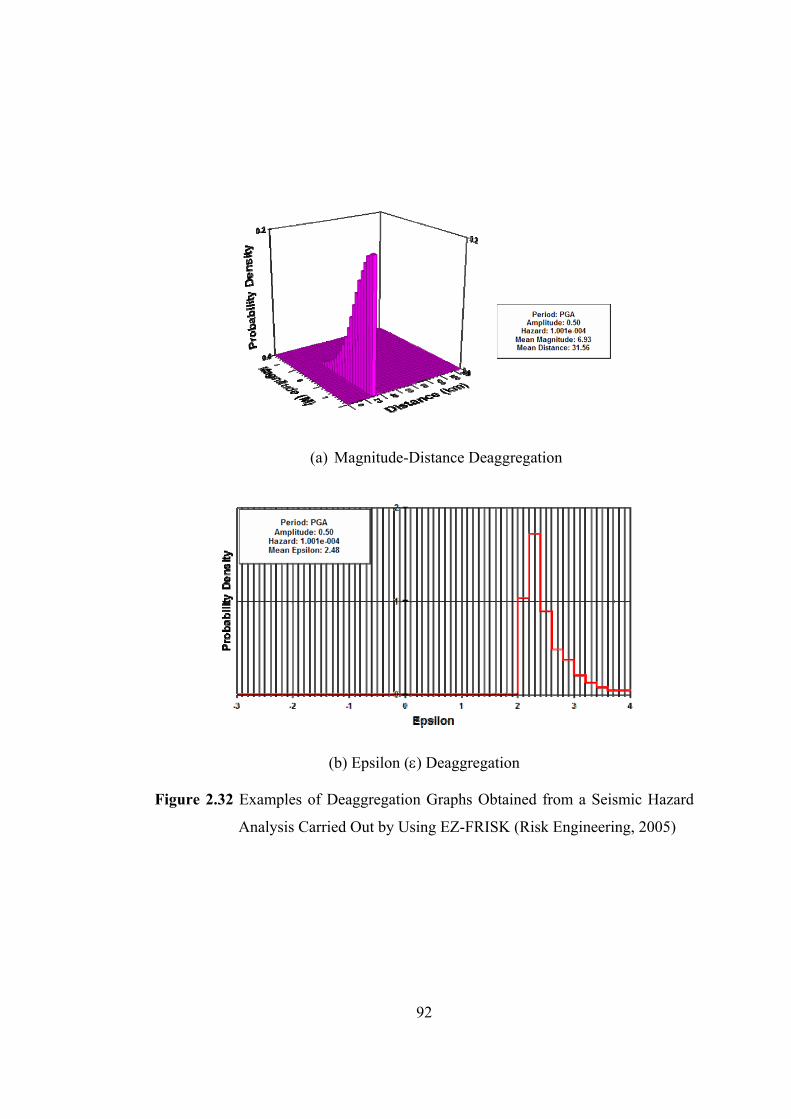
92
(a) Magnitude-Distance Deaggregation
(b) Epsilon (ε) Deaggregation Figure 2.32 Examples of Deaggregation Graphs Obtained from a Seismic Hazard
Analysis Carried Out by Using EZ-FRISK (Risk Engineering, 2005)
93
CHAPTER 3
CASE STUDY FOR A COUNTRY: SEISMIC HAZARD MAPPING FOR JORDAN
3.1 INTRODUCTION In the previous chapter, the basic inputs of the probabilistic seismic hazard analysis
model are explained in detail and the treatment of the related uncertainties is
discussed. The sensitivity of results to the various inputs are examined by
considering a line source (fault) and sites of varying distances to this fault.
As mentioned earlier, in developing seismic hazard maps or updating the existing
ones, it is necessary to take into consideration the seismic hazard nucleating from
faults. This requires the assessment of the main parameters of the faults. However,
this process requires time and it is quite expensive if it is carried out for large
regions like a country. This fact is observed in the study conducted for the
development of the current earthquake zoning map of Turkey, where all seismic
sources were defined as area sources.
In this chapter, a case study will be carried out to illustrate how seismic hazard
analysis should be carried out for the seismic hazard assessment of the regions for
which the data is not adequate to apply the more complex models, such as,
cascading, segmentation and renewal. In certain cases, the locations of faults on the
earth surface may not be well defined to use line source modeling. In such a case,
the simplest models based on area sources and exponential magnitude distribution
can be used in the assessment of seismic hazard. In cases where the exact locations
of faults are defined, line source model combined with exponential magnitude
distribution or characteristic earthquake model can be applied in seismic hazard

94
assessment studies. Besides, purely characteristic earthquake or maximum
magnitude models can be used for faults and the remaining seismicity is to be
considered in seismic hazard calculations by defining a background area source
with uniform seismicity or by applying spatially smoothed seismicity model. In the
case study presented in this chapter, Jordan is selected as the country to examine
sensitivity of seismic hazard results to seismic source modeling and various
assumptions with respect to magnitude distribution.
Most parts of Jordan, especially the regions along the Dead Sea-Jordan rift valley,
are subject to significant seismic threat. Since the major cities and industry are
located in earthquake prone regions, it is quite important to quantify the future
seismic hazard in these regions and design and construct the engineering structures
consistent with the resulting seismic hazard.
3.2 PREVIOUS PROBABILISTIC SEISMIC HAZARD ASSESSMENT
STUDIES FOR JORDAN The earlier probabilistic seismic hazard studies in the region are very limited in
number and they date back to the development of seismic hazard maps for Palestine
(Ben-Menahem, 1981; Shapira, 1981). Later, a number of studies were conducted
for the prediction of seismic hazard in Jordan. Yücemen (1992) conducted a very
comprehensive study for the assessment of the seismic hazard in Jordan and its
vicinity by using probabilistic and statistical methods. Seven seismic sources, which
include line sources for the well defined faults and area sources for others, were
delineated in this study. The results were presented in the form of seismic hazard
maps displaying iso-acceleration and iso-intensity contours corresponding to
different return periods. In that study, the major problems were the identification of
seismic source zones, delineation of faults, assessment of the fault parameters and
the nonavaliability of attenuation relationships derived based on local data.
In a later study conducted by Yücemen (1995), the problems associated with the
location of seismic source zones were addressed in full and a model was described

95
to quantify and incorporate explicitly the errors made in the demarcation of the
source zone boundaries. The basic concept introduced in that model was the
assumption of random source zone boundaries instead of deterministic ones. To
demonstrate the application of the proposed model, seismic hazard was computed at
three different cities in Jordan. The sensitivity of results to the location uncertainty
was examined and a comparison against the previous results was also made.
In the last decade a number of studies (Al-Tarazi, 1992; Batayneh, 1994; Husein
Malkawi et al., 1995; Fahmi et al., 1996) were conducted for the development of
seismic hazard maps for Jordan and its vicinity. The probabilistic methodology and
the computational algorithms were not different than the ones utilized by Yücemen
(1992; 1995), however, these studies enjoyed the benefit of having more
information and expert opinion for the delineation of seismic sources. Accordingly,
more reliable seismic source models and seismicity parameters were used in these
studies.
Jiménez (2004) carried out a comprehensive study for seismic hazard mapping of
Jordan. This study was based on up-to-date information for seismic sources and
seismicity of the region. 18 seismic sources were delineated in the region. They
were modeled as area sources even where faults were well defined based on
geological and seismological investigations in order to evaluate the inherent
uncertainty in hypocenter determination of earthquakes. Narrow area sources were
defined for Dead Sea Transform System while wider sources were used for the
areas having more distributed seismicity. The attenuation relationships proposed by
Ambraseys et al. (1996) for rock sites and for peak ground acceleration (PGA) and
spectral accelerations (SA) for 0.1 sec, 0.2 sec, 0.3 sec, 0.5 sec, 1.0 sec and 2.0 sec
were used in seismic hazard computations. Contour maps were presented to display
predicted PGA and SA values at 10% probability of exceedance in 50 years.
Al-Tarazi and Sandvol (2007) recently conducted a study for seismic hazard
evaluation along the Jordan-Dead Sea Transform. Three models were used to
produce probabilistic seismic hazard maps for the region. Model I and Model II
96
were based on spatially smoothed earthquakes with magnitudes greater than 3.0 for
the time period 1900 to 2003 and magnitude range between 5.0 and 7.0 for the time
period 2100 B.C and A.D. 2003, respectively. No seismic source zones have been
used in these two models. In Model III, contribution of the large events with
magnitude equal to or greater than 7.0 to the seismic hazard is calculated by
assigning them to major faults as characteristic events having a narrow magnitude
range. Three different attenuation relationships proposed by Boore et al. (1997),
Sadigh et al. (1997) and Campbell (1997) for peak ground acceleration at firm rock
sites have been used in calculations and the results were combined by giving equal
weights (0.333) to each one of these relationships. The results obtained from Model
I, Model II and Model III were combined to form a single probabilistic seismic
hazard map. For this purpose, the weights of 0.5 and 0.5 were given to Model I and
Model II, respectively. The probabilities of exceedances obtained from Model III
were added to weighted mean of the probabilities of exceedances from Model I and
Model II. The maps showing the peak ground acceleration with 10 % probability of
exceedance in 50 years were produced for Model I, Model II and Model III as well
as for the combination of them.
3.3 ASSESSMENT OF SEISMIC HAZARD FOR JORDAN 3.3.1 Seismic Database and Seismic Sources Two major steps of PSHA are the delineation of seismic sources and the assessment
of the earthquake occurrence characteristics for each seismic source. Therefore, the
past earthquake catalogs and tectonic structure of the region of interest must be
studied to determine the locations and magnitude-recurrence relationships of
seismic sources that generate the future seismic activity.
3.3.1.1 Seismic Database In order to carry out a seismic hazard analysis for Jordan, the seismicity and
tectonics of the rectangular region bounded by 27-36° N latitudes and 30.4-40° E

97
longitudes is studied. For this region, two earthquake catalogs which are presented
in Jiménez (2004) are used. First earthquake catalog includes the earthquakes that
occurred between the years 0 and 1989. In this study, the historical events that
occurred between the years 0 and 1899 are not taken into consideration due to the
incompleteness in smaller magnitudes. However, it is believed that it can be used to
delineate seismic sources and to determine their maximum magnitudes. The
magnitudes of the events between the years 1900 and 1989 are given in local
magnitude (ML) scale. The earthquake magnitudes in body wave magnitude (Mb)
scale for the events with ML≥4.0 as well as those in surface wave magnitude (Ms)
scale for some events are also presented. The second earthquake catalog includes
the events that occurred between the years 1990 and 1998. The magnitudes of these
events are given in local magnitude scale. Therefore, the whole earthquake catalog
contains events between the years 1900 and 1998.
Peak ground acceleration (PGA) and spectral acceleration (SA) at 0.2 and 1.0
seconds are selected as the basic parameters for the seismic hazard evaluation. The
attenuation equations proposed by Ambraseys et al. (1996) are used to estimate
seismic hazard in terms of these parameters. Since no information is available about
the site conditions all over Jordan, all computations are carried out for rock site
condition. In the equations proposed by Ambraseys et al. (1996), the magnitude
values should be in terms of surface wave magnitude scale, Ms. Therefore, the
magnitudes of earthquakes in the catalog are converted from the local magnitude
scale, ML, to Ms by using the equation derived by Jiménez (2004) based on
earthquake catalog compiled for the seismic hazard assessment of Jordan as given
below:
50.0M11.1M Ls −= (3.1) Poisson model assumes independence between the earthquakes. Therefore,
secondary events; i.e. foreshocks and aftershocks sequences, should be removed
from the earthquake catalog. Various methods are proposed in literature to identify
secondary events. The simple one is that the earthquakes that fall into space and
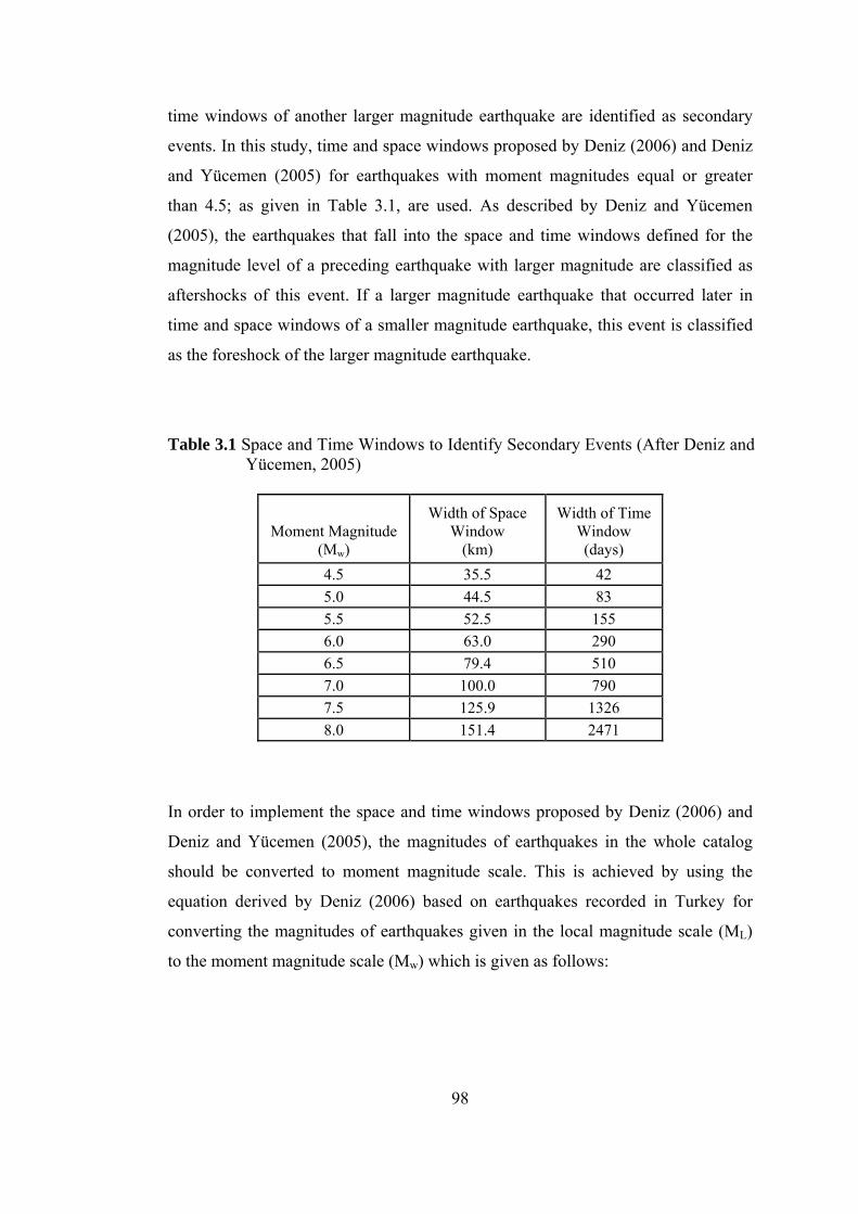
98
time windows of another larger magnitude earthquake are identified as secondary
events. In this study, time and space windows proposed by Deniz (2006) and Deniz
and Yücemen (2005) for earthquakes with moment magnitudes equal or greater
than 4.5; as given in Table 3.1, are used. As described by Deniz and Yücemen
(2005), the earthquakes that fall into the space and time windows defined for the
magnitude level of a preceding earthquake with larger magnitude are classified as
aftershocks of this event. If a larger magnitude earthquake that occurred later in
time and space windows of a smaller magnitude earthquake, this event is classified
as the foreshock of the larger magnitude earthquake.
Table 3.1 Space and Time Windows to Identify Secondary Events (After Deniz and
Yücemen, 2005)
Moment Magnitude (Mw)
Width of Space Window
(km)
Width of Time Window (days)
4.5 35.5 42 5.0 44.5 83 5.5 52.5 155 6.0 63.0 290 6.5 79.4 510 7.0 100.0 790 7.5 125.9 1326 8.0 151.4 2471
In order to implement the space and time windows proposed by Deniz (2006) and
Deniz and Yücemen (2005), the magnitudes of earthquakes in the whole catalog
should be converted to moment magnitude scale. This is achieved by using the
equation derived by Deniz (2006) based on earthquakes recorded in Turkey for
converting the magnitudes of earthquakes given in the local magnitude scale (ML)
to the moment magnitude scale (Mw) which is given as follows:

99
66.2M57.1M Lw −= (3.2) The minimum magnitude earthquake, m0, to be considered in seismic hazard
analysis is set equal to 4.0 in surface wave magnitude scale (Ms). Therefore,
earthquakes with moment magnitude less than 3.6, which corresponds to 3.93 in
surface magnitude scale according to Eqs. (3.1) and (3.2), are removed from the
earthquake catalog.
A computer program is coded in order to apply the secondary event identification
procedure explained above. The earthquake catalog and time and space windows of
earthquake magnitudes defined for earthquakes in the catalog are inputs for this
program. For magnitudes that are not given in Table 3.1, the linear and log-linear
interpolations are applied for duration and distance values, respectively. Since the
distance and duration windows are given for moment magnitudes equal to or greater
than 4.5, some extrapolations are made to define windows for magnitudes less than
this value. Besides, the earthquakes with magnitudes greater than 6.0 are assumed
to be main shocks although they may be identified as secondary events of another
main shock. The resulting earthquake catalog includes 175 main shocks, which can
be treated as independent events, are listed in Appendix B. The spatial distribution
of earthquakes in the resulting catalog is shown in Figure 3.1.
3.3.1.2 Seismic Sources The Dead Sea Transform Fault System (DSTFS) which extends in approximately
south-north direction near the west boundary of Jordan produced very destructive
earthquakes since pre-historical times (Ben-Menahem, 1979). The DSTFS was
formed as a result of the breakup of the Arabian plate from the African plate
(Barazangi, 1983). Deformation in this boundary is intense and complex with faults
trending not only sub parallel to the transform but also oblique to it (Bender, 1974).
The tectonic setting of Dead Sea transform fault system is shown in Figure 3.2.

100
32° 34° 36° 38° 40°
32° 34° 36° 38° 40°
28°
30°
32°
34°
36°
28°
30°
32°
34°
36°
Figure 3.1 Map Showing the Spatial Distribution of Main Shocks in the Catalog
Compiled for the Seismic Hazard Assessment of Jordan The Dead Sea transform system extends from the Gulf of Aqaba in the south
through Wadi Araba, Dead Sea Basin and continues in the north direction through
Yammouneh and Ghab faults that intersects with the Arabia-Eurasia collision zone
in southern Turkey (Al-Tarazi and Sandvol, 2007). This system has left-lateral en-
echelon strike-slip faults that produced several deep pull-apart basins. The Dead Sea
and Gulf of Aqaba are the larger ones among them (Ben-Avraham, 1985).
In this study, two different models, namely area and line, are used for the main
seismic sources that affect Jordan. For the location of seismic sources, the
information given in the report by Jiménez (2004) is used. The locations of area
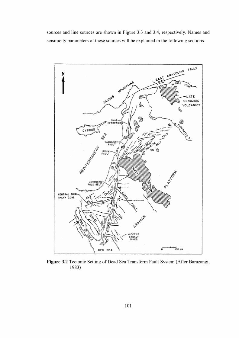
101
sources and line sources are shown in Figure 3.3 and 3.4, respectively. Names and
seismicity parameters of these sources will be explained in the following sections.
Figure 3.2 Tectonic Setting of Dead Sea Transform Fault System (After Barazangi, 1983)

102
32° 34° 36° 38° 40°
28°
30°
32°
34°
36° 32° 34° 36° 38° 40°
28°
30°
32°
34°
36°
18
15 17
16
7
6
5 12
11
10
8
43
1
213
14
9
Figure 3.3 Locations of Area Sources Used in This Study (After Jiménez, 2004)
32° 34° 36° 38° 40°
28°
30°
32°
34°
36° 32° 34° 36° 38° 40°
28°
30°
32°
34°
36°
13
14
11
12
54 10
9
8
6
3
17
2
Mediterranean Sea
Figure 3.4 Locations of Line Sources Used in This Study (After Jiménez, 2004)
103
3.3.2 Alternative Models Different seismic source models combined with different magnitude recurrence
relationships are applied to calculate seismic hazard for Jordan. These models will
be explained starting from the simplest to the more complex ones in the following
sections.
3.3.2.1 Model 1 This is the simplest model compared with the others. The area sources shown in
Figure 3.3 are used by assuming exponential magnitude distribution for all of them.
The lower bound magnitude (m0) is taken as 4.0 for all sources. The annual rate (ν)
and slope of the exponential magnitude distribution (β) are assessed based on the
information given in the report by Jiménez (2004) since this study appears to be the
most comprehensive one and has compiled up-to-date information. However, a
certain degree of cross checking has also been done by using some of the other
references (Yücemen, 1992; Al-Tarazi, 1992; Batayneh, 1994; Fahmi et al., 1996).
The depths of seismic sources except those defined for Cyprus and Gulf of Suez are
assumed to be 20 km based on the study of Al-Tarazi and Sandvol (2007). The
depth for the Cyprus area source is taken as 40 km which is the average value of the
depths of the earthquakes that are listed in the earthquake catalog which includes
only the main shocks and fall into this source. Similarly, the depths of two seismic
sources defined for Gulf of Suez, namely Gulf of Suez-North and Gulf of Suez-
South, are taken as 25 km which is consistent with the study of Al-Tarazi and
Sandvol (2007). In the earthquake catalog, there exist some events that cannot be
associated with any one of the seismic sources identified in this model. These
activities are treated as the background seismicity and its effect is smeared over the
whole region. For the background seismic source, the parameter of the exponential
magnitude distribution, β, is taken from the study of Yücemen (1992). The
seismicity parameters of the seismic sources in Model 1 are listed in Table 3.2.

104
Table 3.2 Parameters of Seismic Sources Considered in Model 1
ν Depth Source No.* Name of Source m1 (per year) |β| (km) 1 Dead Sea-Jordan River 7.5 0.33 1.73 20 2 Wadi-Araba 6.6 0.11 1.89 20 3 Yamune-Roum 8.0 1.47 2.12 20 4 Palmira 6.0 0.12 2.21 20 5 Gulf of Aqaba 6.5 1.51 1.96 20 6 Gulf of Suez-South 7.0 0.54 2.46 25 7 Gulf of Suez-North 7.0 0.19 1.84 25 8 Sirhan Faults 7.0 0.05 1.63 20 9 Farah Haifa 5.8 0.09 1.98 20 10 Wadi Karak 4.7 0.023 1.01 20 11 SE Maan 4.6 0.029 0.67 20 12 East Gulf of Aqaba 5.9 0.054 0.92 20 13 Central Sinai 4.0 0.01 0.69 20 14 North East Gaza 4.5 0.022 0.78 20 15 SE-Mediterranean 1 5.8 1.75 1.84 20 16 SE-Mediterranean 2 5.8 0.49 2.42 20 17 SE-Mediterranean 3 7.5 0.09 2.12 20 18 Cyprus 8.0 2.74 2.26 40 Background 5.0 0.49 1.75 20
* These numbers correspond to the source numbers shown in Figure 3.3.
3.3.2.2 Model 2 and Model 3 In Model 2, all seismic sources, except SE-Mediterranean 1, SE-Mediterranean 2,
SE-Mediterranean 3 and Cyprus, are modeled as line (fault) sources as shown in
Figure 3.4. The lower bound magnitude (m0) is taken as 4.0 for all sources. Similar
to Model 1, a background area source is defined to take into account the seismic
activity that cannot be related with any one of the seismic sources in this model.
Exponential magnitude distribution is assumed for all sources.
In Model 3, same seismic sources and seismicity parameters are used. But,
characteristic earthquake model proposed by Youngs and Coppersmith (1985) is
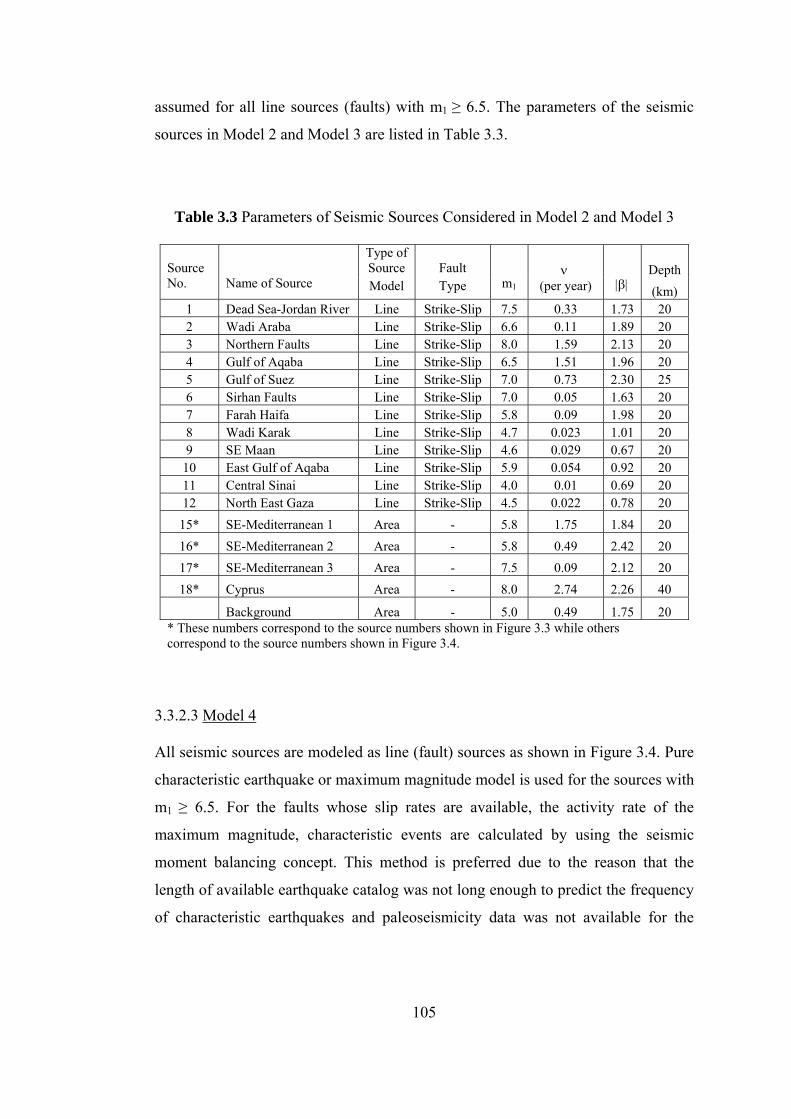
105
assumed for all line sources (faults) with m1 ≥ 6.5. The parameters of the seismic
sources in Model 2 and Model 3 are listed in Table 3.3.
Table 3.3 Parameters of Seismic Sources Considered in Model 2 and Model 3
Type of Source
Fault
ν Depth
Source No.
Name of Source Model Type
m1 (per year)
|β| (km) 1 Dead Sea-Jordan River Line Strike-Slip 7.5 0.33 1.73 20 2 Wadi Araba Line Strike-Slip 6.6 0.11 1.89 20 3 Northern Faults Line Strike-Slip 8.0 1.59 2.13 20 4 Gulf of Aqaba Line Strike-Slip 6.5 1.51 1.96 20 5 Gulf of Suez Line Strike-Slip 7.0 0.73 2.30 25 6 Sirhan Faults Line Strike-Slip 7.0 0.05 1.63 20 7 Farah Haifa Line Strike-Slip 5.8 0.09 1.98 20 8 Wadi Karak Line Strike-Slip 4.7 0.023 1.01 20 9 SE Maan Line Strike-Slip 4.6 0.029 0.67 20
10 East Gulf of Aqaba Line Strike-Slip 5.9 0.054 0.92 20 11 Central Sinai Line Strike-Slip 4.0 0.01 0.69 20 12 North East Gaza Line Strike-Slip 4.5 0.022 0.78 20
15* SE-Mediterranean 1 Area - 5.8 1.75 1.84 20 16* SE-Mediterranean 2 Area - 5.8 0.49 2.42 20 17* SE-Mediterranean 3 Area - 7.5 0.09 2.12 20 18* Cyprus Area - 8.0 2.74 2.26 40
Background Area - 5.0 0.49 1.75 20 * These numbers correspond to the source numbers shown in Figure 3.3 while others correspond to the source numbers shown in Figure 3.4.
3.3.2.3 Model 4 All seismic sources are modeled as line (fault) sources as shown in Figure 3.4. Pure
characteristic earthquake or maximum magnitude model is used for the sources with
m1 ≥ 6.5. For the faults whose slip rates are available, the activity rate of the
maximum magnitude, characteristic events are calculated by using the seismic
moment balancing concept. This method is preferred due to the reason that the
length of available earthquake catalog was not long enough to predict the frequency
of characteristic earthquakes and paleoseismicity data was not available for the

106
faults considered. Seismic moment, first introduced by Aki (1966), describes size of
an earthquake with static fault parameters as follows:
ADM0 μ= (3.3) where, M0 is the seismic moment, μ is the rigidity or shear modulus of the crust
(usually taken as 3.0 x 10¹¹ dyne/cm2), A is the rupture area on the fault plane
undergoing slip during the earthquake, and D is average displacement over the slip
surface.
The seismic moment rate, M0
′, or the rate of seismic energy release can be
calculated from the time derivative of Eq. (3.3) as follows:
ASM0 μ=′ (3.4) where M0
′ is the seismic moment rate and S is the average slip-rate along the fault.
Seismic moment can be calculated from the moment magnitude, Mw, by using the
following equation (Hanks and Kanamori, 1979):
Mw = 2/3 logM0-10.7 (3.5) or
05.16M5.1
0 w10M += (3.6) The activity rate of earthquakes with magnitude, Mw, can be calculated from the
combination of Eqs. (3.4) and (3.6) in the following form;
05.16M5.10
0M
w10AS
MM
+μ
=′
=ν (3.7)
Based on the study of Ambraseys (2006), average slip rate of 4.5 mm/year is
assigned to the faults that constitutes the main Dead Sea fault system and extends in
approximately south-north direction although it may be somewhat larger in the
107
north and smaller in the south. This value is also consistent with the slip rate
distribution given by Mahmoud et al. (2005). For the Gulf of Suez and Cyprus
faults, the slip-rate distribution of Mahmoud et al. (2005) is applied.
The seismic moment in the denominator of Eq. (3.7) is calculated from the moment
magnitude scale. But, maximum magnitudes of the faults considered in this study
are given in surface wave magnitude scale. Hanks and Kanamori (1979) stated that
Eq. (3.5) is uniformly valid for 5.0 ≤ Ms ≤ 7.5. Except Cyprus Fault, maximum
magnitudes of the faults for which slip rates are available are in this range. In
addition, Ambraseys (2001) proposed the following equation for Eastern
Mediterranean and Middle East Region to calculate seismic moment from surface
wave magnitude scale, Ms, greater than 6.0;
s0 M5.107.16Mlog += (3.8) The constants in Eq. (3.8) are approximately the same with those given by Hanks
and Kanamori (1979). Therefore, the maximum magnitudes of the faults are not
converted from surface wave magnitude scale to moment magnitude scale in order
to calculate the activity rate of maximum magnitude earthquakes from Eq. (3.7).
For the rest of the faults with m1 ≥ 6.5, the activity rate of maximum magnitude
events are taken as equal to the rate associated with characteristic earthquakes over
the interval (m1, m1–0.5) in characteristic earthquake model proposed by Youngs
and Coppersmith (1985). For the faults with m1<6.5, exponential magnitude
distribution is used and the lower bound, m0, is set equal to 4.0. The parameters of
the faults in Model 4 are listed in Table 3.4.

108

109
The earthquakes that are not assigned to any one of the specific faults are assumed
to be potential seismogenic sources and the contribution of these events to seismic
hazard is calculated by using the spatially smoothed seismicity model of Frankel
(1995). The earthquakes with magnitudes between 4.0 and 6.5 in the catalog
including only main shocks are used in this model. Also, the earthquakes related
with the faults having maximum magnitudes less than 6.5 are eliminated from the
catalog. Figure 3.5 shows the distribution of earthquakes used in spatially smoothed
seismicity model. The slope of the Gutenberg-Richter magnitude recurrence
relationship, b, is computed as 0.71 based on this dataset. Figure 3.6 shows the
magnitude-recurrence relationship derived as well as the data used.
32° 34° 36° 38° 40°
32° 34° 36° 38° 40°
28°
30°
32°
34°
36°
28°
30°
32°
34°
36°
Figure 3.5 Map Showing the Distribution of Earthquakes Used in Spatially
Smoothed Seismicity Model and Locations of the Cities for Which Seismic Hazard are Computed

110
0
0.5
1
1.5
2
2.5
4 4.5 5 5.5 6 6.5 7
Magnitude, m
Log
N(m
)
log N(m)=5.09-0.71mR2=0.9676
Figure 3.6 Magnitude-Recurrence Relationship Derived from the Data Used in
Spatially Smoothed Seismicity Model The region studied is divided into cells of a grid with spacing of 0.1° x 0.1° in
latitude and longitude. The number of earthquakes with magnitude equal to or
greater than 4.0 are counted in each cell. Then, these cumulative values are
converted to incremental values using the formula by Hermann (1977) and spatially
smoothed over a grid of 0.1° x 0.1° in latitude and longitude by using a Gaussian
function having a correlation distance, c, of 50 km. The computations are carried
out by using the computer program developed by USGS (Frankel et al., 1996) and
modified by Kalkan (2007) in order to include additional attenuation relationships.
3.3.3 Seismic Hazard Computations Seismic hazard analyses are carried out by using the models described in Section
3.3.2. EZ-FRISK (Risk Engineering, 2005) software is used to calculate seismic
hazard nucleating from the main seismic sources (line and area sources) and
background seismic source with uniformly distributed seismicity while the
computer program developed by USGS (Frankel et al., 1996) is used to quantify the

111
seismic hazard based on the spatially smoothed seismicity model. For Model 4, the
results of analyses obtained from these two computer programs are combined
externally by summing annual exceedance probabilities corresponding to the same
ground motion parameter (PGA or SA) level at each site and calculating the values
corresponding to the selected return period. In order to achieve this, a computer
program is coded.
Four sites which are located in Azraq, Amman, Irbid and Aqaba are selected. The
sites corresponding to these cities are marked on Figure 3.4. Figures 3.7 through
3.10 show seismic hazard curves obtained for PGA at these sites according the four
models explained in the previous section. It can be observed from these figures that
modeling the faults as area sources coupled with exponential magnitude distribution
(Model 1) resulted in the lowest annual exceedance probabilities for PGA values
greater than 0.03g at all sites. On the other hand, modeling the faults, except
Cyprus, SE-Mediterranean 1, SE-Mediterranean 2 and SE-Mediterranean 3, as line
sources with exponential magnitude distribution (Model 2) gave higher seismic
hazard results compared to Model 1 as expected, since the rates are distributed over
the areas in Model 1 instead of those assigned along the fault lines in Model 2. The
use of characteristic earthquake model proposed by Youngs and Coppersmith
(1985) for major faults with magnitude, m ≥ 6.5 (Model 3) resulted in higher
seismic hazard results compared to the exponentially distributed magnitude
assumption. This is due to the increased rate in large magnitude earthquakes
consistent with the characteristic earthquake model. Compared with Model 3,
modeling all faults as line sources and applying purely characteristic or maximum
magnitude model for magnitude distribution of faults with magnitude, m ≥ 6.5,
combined with spatially smoothed seismicity model for earthquakes with m<6.5
(Model 4) resulted in lower exceedance probabilities up to certain PGA levels. For
the PGA values larger than these levels, the opposite trend is valid.
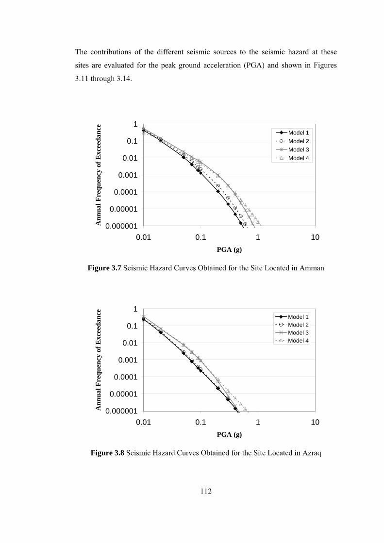
112
The contributions of the different seismic sources to the seismic hazard at these
sites are evaluated for the peak ground acceleration (PGA) and shown in Figures
3.11 through 3.14.
0.000001
0.00001
0.0001
0.001
0.01
0.1
1
0.01 0.1 1 10PGA (g)
Ann
ual F
requ
ency
of E
xcee
danc
e
Model 1Model 2Model 3Model 4
Figure 3.7 Seismic Hazard Curves Obtained for the Site Located in Amman
0.000001
0.00001
0.0001
0.001
0.01
0.1
1
0.01 0.1 1 10PGA (g)
Ann
ual F
requ
ency
of E
xcee
danc
e
Model 1Model 2Model 3Model 4
Figure 3.8 Seismic Hazard Curves Obtained for the Site Located in Azraq

113
0.000001
0.00001
0.0001
0.001
0.01
0.1
1
0.01 0.1 1 10PGA (g)
Ann
ual F
requ
ency
of E
xcee
danc
e
Model 1Model 2Model 3Model 4
Figure 3.9 Seismic Hazard Curves Obtained for the Site Located in Aqaba
0.000001
0.00001
0.0001
0.001
0.01
0.1
1
0.01 0.1 1 10PGA (g)
Ann
ual F
requ
ency
of E
xcee
danc
e
Model 1Model 2Model 3Model 4
Figure 3.10 Seismic Hazard Curves Obtained for the Site Located in Irbid

114
0.000001
0.00001
0.0001
0.001
0.01
0.1
1
0.01 0.1 1
PGA(g)
Ann
ual F
requ
ency
of E
xcee
danc
e
Dead Sea-Jordan River
Wadi Araba
Yamune Roum
Sirhan Faults
Farah Haifa
Wadi Karak
SE-Mediterranean 2
SE-Mediterranean 3
Cyprus
Background
TOTAL
(a) Model 1
0.000001
0.00001
0.0001
0.001
0.01
0.1
1
0.01 0.1 1
PGA(g)
Ann
ual F
requ
ency
of E
xcee
danc
e
Dead Sea-Jordan River
Wadi Araba
Northern Faults
Sirhan Faults
Farah Haifa
Wadi Karak
SE-Mediterranean 2
SE-Mediterranean 3
Cyprus
Background
TOTAL
(b) Model 2
Figure 3.11 Contributions of the Different Seismic Sources to the Seismic Hazard
at the Site Located in Amman

115
0.000001
0.00001
0.0001
0.001
0.01
0.1
1
0.01 0.1 1
PGA(g)
Ann
ual F
requ
ency
of E
xcee
danc
e
Dead Sea-Jordan River
Wadi Araba
Northern Faults
Gulf of Aqaba
Gulf of Suez
Sirhan Faults
Farah Haifa
Wadi Karak
SE-Mediterranean 2
SE-Mediterranean 3
Cyprus
Background
TOTAL
(c) Model 3
0.000001
0.00001
0.0001
0.001
0.01
0.1
1
0.01 0.1 1 10
PGA(g)
Ann
ual F
requ
ency
of E
xcee
danc
e
Dead Sea-Jordan River
Wadi Araba
Northern Faults
Gulf of Aqaba
Gulf of Suez
Sirhan Faults
Farah Haifa
Wadi Karak
SE-Mediterranean
Cyprus
Spatially Smooth Seismicity
TOTAL
(d) Model 4
Figure 3.11(Continued) Contributions of the Different Seismic Sources to the
Seismic Hazard at the Site Located in Amman
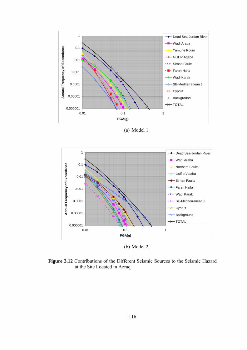
116
0.000001
0.00001
0.0001
0.001
0.01
0.1
1
0.01 0.1 1
PGA(g)
Ann
ual F
requ
ency
of E
xcee
danc
e
Dead Sea-Jordan River
Wadi Araba
Yamune Roum
Gulf of Aqaba
Sirhan Faults
Farah Haifa
Wadi Karak
SE-Mediterranean 3
Cyprus
Background
TOTAL
(a) Model 1
0.000001
0.00001
0.0001
0.001
0.01
0.1
1
0.01 0.1 1
PGA(g)
Ann
ual F
requ
ency
of E
xcee
danc
e
Dead Sea-Jordan River
Wadi Araba
Northern Faults
Gulf of Aqaba
Sirhan Faults
Farah Haifa
Wadi Karak
SE-Mediterranean 3
Cyprus
Background
TOTAL
(b) Model 2
Figure 3.12 Contributions of the Different Seismic Sources to the Seismic Hazard
at the Site Located in Azraq

117
0.000001
0.00001
0.0001
0.001
0.01
0.1
1
0.01 0.1 1
PGA(g)
Ann
ual F
requ
ency
of E
xcee
danc
e
Dead Sea-Jordan River
Wadi Araba
Northern Faults
Gulf of Aqaba
Sirhan Faults
Farah Haifa
Wadi Karak
SE-Mediterranean 3
Cyprus
Background
TOTAL
(c) Model 3
0.000001
0.00001
0.0001
0.001
0.01
0.1
1
0.01 0.1 1
PGA(g)
Ann
ual F
requ
ency
of E
xcee
danc
e
Dead Sea-Jordan River
Wadi Araba
Northern Faults
Gulf of Aqaba
Gulf of Suez
Sirhan Faults
Farah Haifa
Wadi Karak
SE-Mediterranean
Cyprus
Spatially Smooth Seismicity
TOTAL
(d) Model 4
Figure 3.12(Continued) Contributions of the Different Seismic Sources to the Seismic Hazard at the Site Located in Azraq

118
0.000001
0.00001
0.0001
0.001
0.01
0.1
1
0.01 0.1 1
PGA(g)
Ann
ual F
requ
ency
of E
xcee
danc
e
Dead Sea-Jordan River
Wadi Araba
Yamune Roum
Gulf of Aqaba
Gulf of Suez-South
Gulf of Suez-North
Sirhan Faults
East Gulf of Aqaba
Cyprus
Background
TOTAL
(a) Model 1
0.000001
0.00001
0.0001
0.001
0.01
0.1
1
0.01 0.1 1
PGA(g)
Ann
ual F
requ
ency
of E
xcee
danc
e
Dead Sea-Jordan River
Wadi Araba
Northern Faults
Gulf of Aqaba
Gulf of Suez
Sirhan Faults
SE Maan
East Gulf of Aqaba
SE-Mediterranean 3
Cyprus
Background
TOTAL
(b) Model 2
Figure 3.13 Contributions of the Different Seismic Sources to the Seismic Hazard
at the Site Located in Aqaba

119
0.000001
0.00001
0.0001
0.001
0.01
0.1
1
0.01 0.1 1 10
PGA(g)
Ann
ual F
requ
ency
of E
xcee
danc
e
Dead Sea-Jordan River
Wadi Araba
Northern Faults
Gulf of Aqaba
Gulf of Suez
Sirhan Faults
SE Maan
East Gulf of Aqaba
SE-Mediterranean 3
Cyprus
Background
TOTAL
(c) Model 3
0.000001
0.00001
0.0001
0.001
0.01
0.1
1
0.01 0.1 1 10
PGA(g)
Ann
ual F
requ
ency
of E
xcee
danc
e
Dead Sea-Jordan River
Wadi Araba
Northern Faults
Gulf of Aqaba
Gulf of Suez
Sirhan Faults
SE Maan
East Gulf of Aqaba
SE-Mediterranean
Cyprus
Spatially Smooth Seismicity
TOTAL
(d) Model 4
Figure 3.13(Continued) Contributions of the Different Seismic Sources to the
Seismic Hazard at the Site Located in Aqaba

120
0.000001
0.00001
0.0001
0.001
0.01
0.1
1
0.01 0.1 1
PGA(g)
Ann
ual F
requ
ency
of E
xcee
danc
e
Dead Sea-Jordan River
Wadi Araba
Yamune Roum
Palmira
Sirhan Faults
Farah Haifa
SE-Mediterranean 2
SE-Mediterranean 3
Cyprus
Background
TOTAL
(a) Model 1
0.000001
0.00001
0.0001
0.001
0.01
0.1
1
0.01 0.1 1
PGA(g)
Ann
ual F
requ
ency
of E
xcee
danc
e
Dead Sea-Jordan River
Wadi Araba
Northern Faults
Gulf of Aqaba
Sirhan Faults
Farah Haifa
SE-Mediterranean 2
SE-Mediterranean 3
Cyprus
Background
TOTAL
(b) Model 2
Figure 3.14 Contributions of the Different Seismic Sources to the Seismic Hazard
at the Site Located in Irbid

121
0.000001
0.00001
0.0001
0.001
0.01
0.1
1
0.01 0.1 1 10
PGA(g)
Ann
ual F
requ
ency
of E
xcee
danc
e
Dead Sea-Jordan River
Wadi Araba
Northern Faults
Gulf of Aqaba
Sirhan Faults
Farah Haifa
SE-Mediterranean 2
SE-Mediterranean 3
Cyprus
Background
TOTAL
(c) Model 3
0.000001
0.00001
0.0001
0.001
0.01
0.1
1
0.01 0.1 1 10
PGA(g)
Ann
ual F
requ
ency
of E
xcee
danc
e
Dead Sea-Jordan River
Wadi Araba
Northern Faults
Gulf of Aqaba
Gulf of Suez
Sirhan Faults
Farah Haifa
North East Gaza
SE-Mediterranean
Cyprus
Spatially Smooth Seismicity
TOTAL
(d) Model 4
Figure 3.14(Continued) Contributions of The Different Seismic Sources to the
Seismic Hazard at the Site Located in Irbid

122
The highest contributing seismic source to the seismic hazards at the sites located in
Amman and Irbid is the Dead Sea-Jordan River in Models 1, 2 and 3. For the site
located in Amman, the background seismic activity modeled as spatially smoothed
seismicity contributes most to the seismic hazard estimated from Model 4. For the
site located in Irbid, background seismic activity for PGA values up to about 0.15g,
and then the Dead Sea-Jordan River fault contribute most to the seismic hazard
predicted by using Model 4. For the site located in Azraq, the highest contributing
seismic source in Models 1, 2 and 3 is the Dead Sea-Jordan River for PGA values
less than about 0.1g, 0.15g and 0.25g, respectively. At the same time, background is
the most effective source to seismic hazard for larger PGA values. For the site
located in Aqaba, Wadi Araba fault is the most effective source for PGA values
greater than about 0.15g, 0.5g and 0.8g in Models 1, 2 and 3, respectively. For
smaller PGA values, Gulf of Aqaba contributes most to the seismic hazard. For
Model 4, background seismic activity modeled as spatially smoothed seismicity,
Gulf of Aqaba and Wadi Araba are the main contributors to the seismic hazard at
the site located in Aqaba.
PGA and SA (T= 0.2 sec and 1.0 sec ) values corresponding to return periods of
475, 1000 and 2475 years are presented in Table 3.5 for the sites in Azraq, Amman,
Irbid and Aqaba. These return periods correspond, respectively, to 10%, 5% and 2%
probabilities of exceedance in 50 years. It is shown in Table 3.5 that for the sites
located in Azraq, Model 1 and Model 2 give nearly same results. This is due to the
reason that most of the seismic hazard in these models resulted from the Dead Sea-
Jordan River source and compared with other sites, this site is located far away
from this source. Therefore, modeling this source as line or area has a negligible
effect on the results for the site in Azraq. For the sites located in Amman, Irbid and
Aqaba, Model 2 gives higher seismic hazard values than Model 1. Among these
cities, the difference is small for Amman, larger for Irbid and largest for Aqaba.
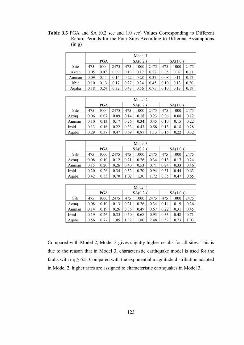
123
Table 3.5 PGA and SA (0.2 sec and 1.0 sec) Values Corresponding to Different Return Periods for the Four Sites According to Different Assumptions (in g)
Model 1
PGA SA(0.2 s) SA(1.0 s) Site 475 1000 2475 475 1000 2475 475 1000 2475
Azraq 0.05 0.07 0.09 0.13 0.17 0.22 0.05 0.07 0.11 Amman 0.09 0.11 0.14 0.22 0.28 0.37 0.08 0.11 0.17
Irbid 0.10 0.13 0.17 0.27 0.34 0.45 0.10 0.13 0.20 Aqaba 0.18 0.24 0.32 0.43 0.56 0.75 0.10 0.13 0.19
Model 2
PGA SA(0.2 s) SA(1.0 s) Site 475 1000 2475 475 1000 2475 475 1000 2475
Azraq 0.06 0.07 0.09 0.14 0.18 0.23 0.06 0.08 0.12 Amman 0.10 0.13 0.17 0.26 0.34 0.45 0.10 0.15 0.22 Irbid 0.13 0.16 0.22 0.33 0.43 0.58 0.13 0.18 0.28 Aqaba 0.29 0.37 0.47 0.69 0.87 1.13 0.16 0.22 0.32
Model 3
PGA SA(0.2 s) SA(1.0 s) Site 475 1000 2475 475 1000 2475 475 1000 2475
Azraq 0.08 0.10 0.12 0.21 0.26 0.34 0.13 0.17 0.24 Amman 0.15 0.20 0.26 0.40 0.53 0.71 0.24 0.33 0.46 Irbid 0.20 0.26 0.34 0.52 0.70 0.94 0.31 0.44 0.63 Aqaba 0.42 0.53 0.70 1.02 1.30 1.72 0.35 0.47 0.65
Model 4
PGA SA(0.2 s) SA(1.0 s) Site 475 1000 2475 475 1000 2475 475 1000 2475
Azraq 0.08 0.10 0.13 0.21 0.26 0.34 0.14 0.19 0.26 Amman 0.14 0.19 0.26 0.36 0.49 0.67 0.22 0.31 0.45 Irbid 0.19 0.26 0.35 0.50 0.68 0.93 0.33 0.48 0.71 Aqaba 0.56 0.77 1.05 1.32 1.80 2.48 0.52 0.73 1.03
Compared with Model 2, Model 3 gives slightly higher results for all sites. This is
due to the reason that in Model 3, characteristic earthquake model is used for the
faults with m1 ≥ 6.5. Compared with the exponential magnitude distribution adapted
in Model 2, higher rates are assigned to characteristic earthquakes in Model 3.

124
Model 3 and Model 4 give nearly the same PGA and SA values for the sites in
Azraq, Amman and Irbid. For Aqaba, PGA and SA values estimated from Model 4
are 1.3 to 1.6 times higher than those obtained from Model3.
It should be mentioned that high PGA and SA values are obtained from Model 3
and Model 4 in Table 3.5 for Aqaba. The site selected for Aqaba is located almost
on the top of Wadi Araba fault and very near to Gulf of Aqaba Fault (about 5 km to
the fault). Therefore, the increase in the rates of maximum magnitude earthquakes
of these faults in Model 3 and Model 4 resulted in such high seismic hazard values.
In addition to the analyses carried out for the four sites explained above, seismic
hazard analyses are carried out to construct seismic hazard maps for Jordan in terms
of PGA and SA at 0.2 sec and 1.0 sec for return periods of 475, 1000 and 2475
years. These return periods correspond to 10%, 5% and 2% probabilities of
exceedance in 50 years. The rectangular region bounded by 27-36° N latitudes and
30.4-40° E longitudes is divided into grids with spacing of 0.1° x 0.1° in latitude
and longitude. Seismic hazard computations are carried out at each grid point
according to each one of the set of assumptions classified as Model 1, Model 2,
Model 3 and Model 4, in order to display the spatial distributions of PGA and SA
(T= 0.2 sec and 1.0 sec) values corresponding to 475, 1000 and 2475 years return
periods. The maps constructed based on the results obtained for PGA are presented
in Appendix C. It should be mentioned that only the values given within the
boundaries of Jordan, drawn by thick black lines in these maps, are reliable. This is
due to the fact that additional seismic sources that may contribute to the seismic
hazard at the sites located outside of the boundaries of Jordan are not taken into
consideration in seismic hazard calculations.
In Model 4, the contribution of background events to hazard is calculated by using
the spatially smoothed seismicity model of Frankel (1995) instead of describing a
background area source with uniform seismicity. However, to investigate the
sensitivity of seismic hazard results to background events, seismic hazard analyses
are also carried out by only using a background area source. The lower and upper
125
bounds of earthquake magnitudes are taken as 4.0 and 6.5. The slope of the
exponential distribution, ⎢β⎢, is calculated as 1.63 which corresponds to the b value
(0.71) used for spatially smoothed seismicity model. The annual rate, ν, is
calculated by dividing the number of earthquakes used in spatially smoothed
seismicity model with the time length of the catalog. Figures 3.15 through 3.17
show the seismic hazard maps for PGA obtained by using the spatially smoothed
seismicity model for return periods of 475, 1000, 2475 years, respectively.
In the case of spatially smoothed seismicity model, maximum PGA values (in g)
range from 0 to 0.15, 0.21 and 0.31 for return periods of 475, 1000 and 2475 years,
respectively. The larger values are observed at the regions where the epicenters of
earthquakes cluster and these values decrease as the distance to these regions
increases. In order to visualize this, the epicenters of the earthquakes used in
spatially smoothed seismicity model are placed on the seismic hazard map obtained
by using this model for PGA corresponding to the return period of 2475 years as
shown in Figure 3.18. On the other hand, the maximum PGA values (in g) obtained
from the analyses carried out by using the background seismic source model with
uniform seismicity are 0.06, 0.08 and 0.12 for return periods of 475, 1000, and 2475
years, respectively. These values are fairly smaller than those obtained from the
spatially smoothed seismicity model. Nearly uniform PGA values are observed in
the maps constructed from the analyses carried out based on the background area
source and these values change within narrow ranges. Therefore, background area
source model with uniform seismicity gives higher PGA values than the spatially
smoothed seismicity model at the sites located far away from the regions where the
epicenters of earthquakes cluster. This can be observed from Figure 3.19 which
shows the spatial variation of the difference in PGA values predicted from spatially
smoothed seismicity model with respect to background seismic source with uniform
seismicity for a return period of 2475 years as well as the epicenters of the
earthquakes considered in spatially smoothed seismicity model. In order to
construct the map in Figure 3.19, the difference between the PGA values obtained
from these two models is calculated at each grid point in the rectangular region

126
bounded by 27-36° N latitudes and 30.4-40° E longitudes by using the following
equation;
( ) 100PGA
PGAPGA%Difference
b
bs ×⎟⎟⎠
⎞⎜⎜⎝
⎛ −= (3.9)
where PGAs and PGAb denote the PGA values estimated from spatially smoothed
seismicity model and background area source with uniform seismicity, respectively.
The difference with negative sign (-) means that background area source with
uniform seismicity gives higher PGA values than spatially smoothed seismicity
model and that with positive sign (+) represents the opposite case.
The differences among Models 1, 2, 3 and 4, in terms of PGA, are calculated for the
region within the boundaries of Jordan from the following equation;
( ) 100PGA
PGAPGA%Difference
iModel
iModeljModel ×⎟⎟⎠
⎞⎜⎜⎝
⎛ −= (3.10)
where PGAModel i and PGAModel j are PGA values obtained from Model i and Model
j, respectively. The difference with positive sign (+) indicates that Model j gives
higher PGA values than Model i and that with negative sign (-) represents the
opposite case.
The spatial variation of these differences is shown in Figures 3.20 through 3.28.

127
32° 34° 36° 38° 40°
32° 34° 36° 38° 40°
28°
30°
32°
34°
36°
28°
30°
32°
34°
36°
Figure 3.15 Seismic Hazard Map for PGA (in g) Obtained by Using Spatially Smoothed Seismicity Model for a Return Period of 475 Years
32° 34° 36° 38° 40°
32° 34° 36° 38° 40°
28°
30°
32°
34°
36°
28°
30°
32°
34°
36°
Figure 3.16 Seismic Hazard Map for PGA (in g) Obtained by Using Spatially Smoothed Seismicity Model for a Return Period of 1000 Years

128
32° 34° 36° 38° 40°
32° 34° 36° 38° 40°
28°
30°
32°
34°
36°
28°
30°
32°
34°
36°
Figure 3.17 Seismic Hazard Map for PGA (in g) Obtained by Using Spatially
Smoothed Seismicity Model for a Return Period of 2475 Years
32° 34° 36° 38° 40°
32° 34° 36° 38° 40°
28°
30°
32°
34°
36°
28°
30°
32°
34°
36°
Figure 3.18 Seismic Hazard Map Showing the PGA Values (in g) Obtained by Using Spatially Smoothed Seismicity Model for a Return Period of 2475 Years and Epicenters of Earthquakes Considered in the Assessment of Seismic Hazard
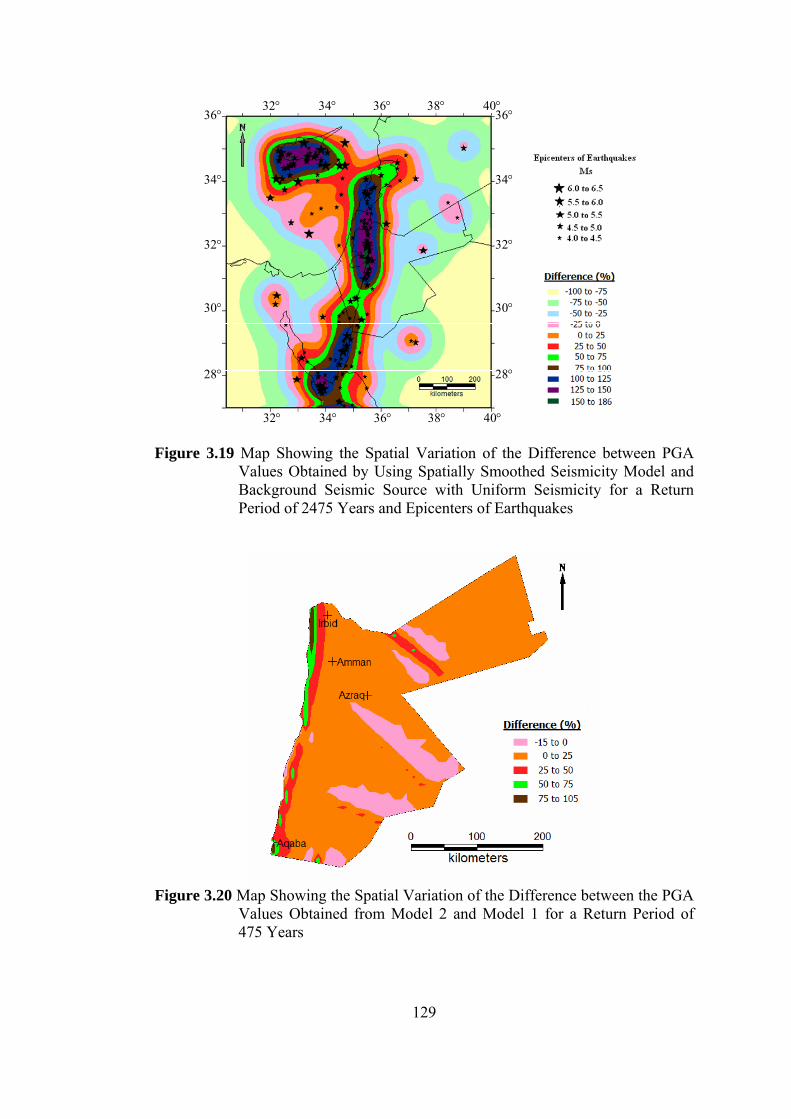
129
32° 34° 36° 38° 40°
32° 34° 36° 38° 40°
28°
30°
32°
34°
36°
28°
30°
32°
34°
36°
Figure 3.19 Map Showing the Spatial Variation of the Difference between PGA
Values Obtained by Using Spatially Smoothed Seismicity Model and Background Seismic Source with Uniform Seismicity for a Return Period of 2475 Years and Epicenters of Earthquakes
Figure 3.20 Map Showing the Spatial Variation of the Difference between the PGA
Values Obtained from Model 2 and Model 1 for a Return Period of 475 Years
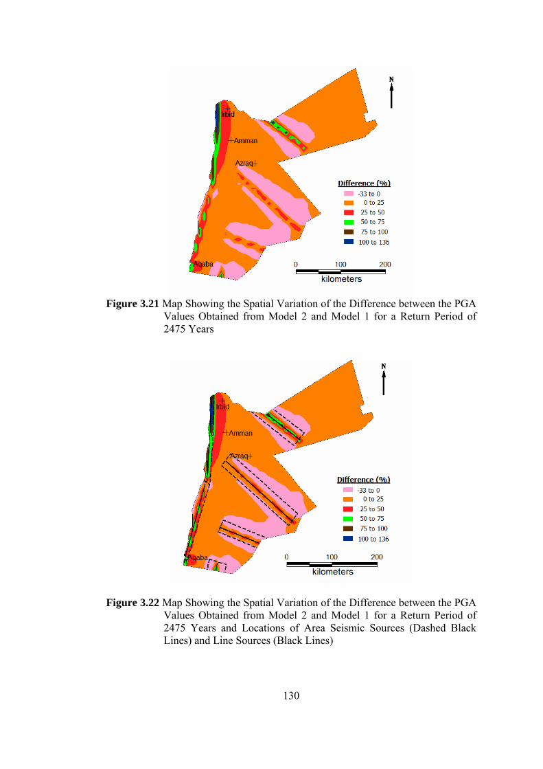
130
Figure 3.21 Map Showing the Spatial Variation of the Difference between the PGA
Values Obtained from Model 2 and Model 1 for a Return Period of 2475 Years
Figure 3.22 Map Showing the Spatial Variation of the Difference between the PGA Values Obtained from Model 2 and Model 1 for a Return Period of 2475 Years and Locations of Area Seismic Sources (Dashed Black Lines) and Line Sources (Black Lines)

131
Figure 3.23 Map Showing the Spatial Variation of the Difference between the PGA
Values Obtained from Model 3 and Model 2 for a Return Period of 475 Years
Figure 3.24 Map Showing the Spatial Variation of the Difference between the PGA
Values Obtained from Model 3 and Model 2 for a Return Period of 2475 Years

132
Figure 3.25 Map Showing the Spatial Variation of the Difference between the PGA
Values Obtained from Model 3 and Model 2 for a Return Period of 2475 Years and Locations of Line Sources (Black Lines)
Figure 3.26 Map Showing the Spatial Variation of the Difference between the PGA
Values Obtained from Model 4 and Model 3 for a Return Period of 475 Years

133
Figure 3.27 Map Showing the Spatial Variation of the Difference between the PGA
Values Obtained from Model 4 and Model 3 for a Return Period of 2475 Years
Figure 3.28 Map Showing the Spatial Variation of the Difference between the PGA Values Obtained from Model 4 and Model 3 for a Return Period of 2475 Years and Locations of Line Sources (Black Lines) and Epicenters of Earthquakes Considered in Spatially Smoothed Seismicity Model
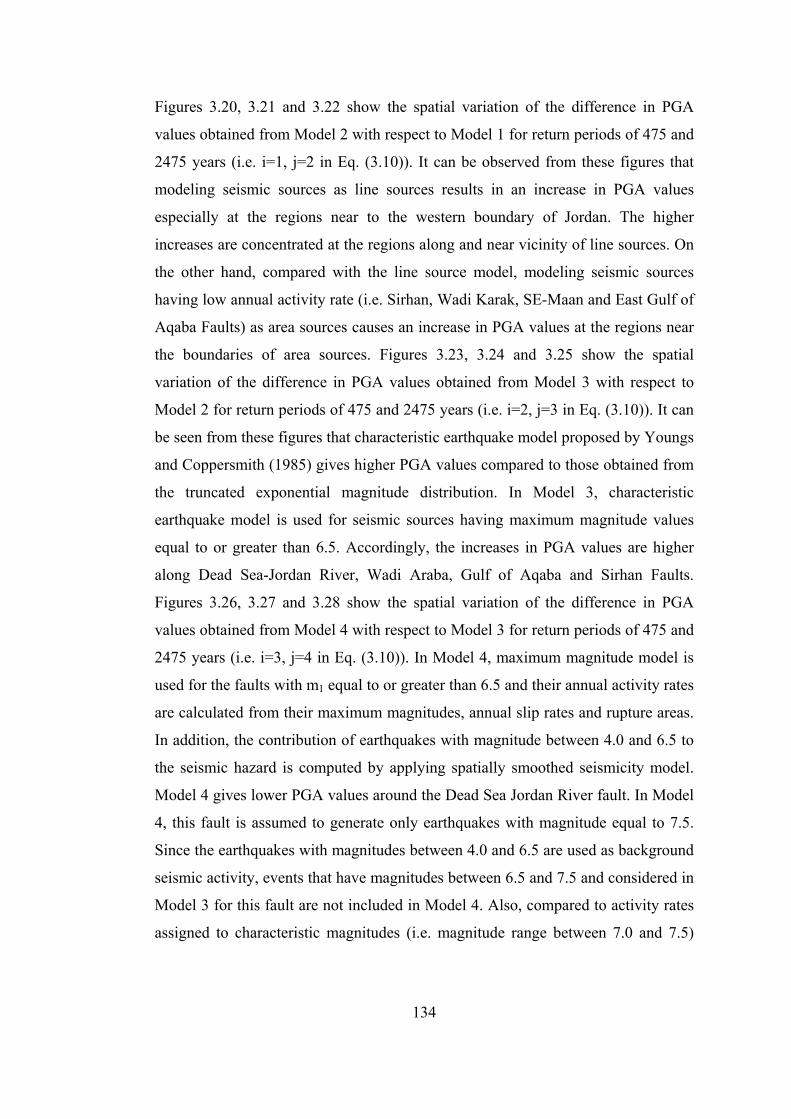
134
Figures 3.20, 3.21 and 3.22 show the spatial variation of the difference in PGA
values obtained from Model 2 with respect to Model 1 for return periods of 475 and
2475 years (i.e. i=1, j=2 in Eq. (3.10)). It can be observed from these figures that
modeling seismic sources as line sources results in an increase in PGA values
especially at the regions near to the western boundary of Jordan. The higher
increases are concentrated at the regions along and near vicinity of line sources. On
the other hand, compared with the line source model, modeling seismic sources
having low annual activity rate (i.e. Sirhan, Wadi Karak, SE-Maan and East Gulf of
Aqaba Faults) as area sources causes an increase in PGA values at the regions near
the boundaries of area sources. Figures 3.23, 3.24 and 3.25 show the spatial
variation of the difference in PGA values obtained from Model 3 with respect to
Model 2 for return periods of 475 and 2475 years (i.e. i=2, j=3 in Eq. (3.10)). It can
be seen from these figures that characteristic earthquake model proposed by Youngs
and Coppersmith (1985) gives higher PGA values compared to those obtained from
the truncated exponential magnitude distribution. In Model 3, characteristic
earthquake model is used for seismic sources having maximum magnitude values
equal to or greater than 6.5. Accordingly, the increases in PGA values are higher
along Dead Sea-Jordan River, Wadi Araba, Gulf of Aqaba and Sirhan Faults.
Figures 3.26, 3.27 and 3.28 show the spatial variation of the difference in PGA
values obtained from Model 4 with respect to Model 3 for return periods of 475 and
2475 years (i.e. i=3, j=4 in Eq. (3.10)). In Model 4, maximum magnitude model is
used for the faults with m1 equal to or greater than 6.5 and their annual activity rates
are calculated from their maximum magnitudes, annual slip rates and rupture areas.
In addition, the contribution of earthquakes with magnitude between 4.0 and 6.5 to
the seismic hazard is computed by applying spatially smoothed seismicity model.
Model 4 gives lower PGA values around the Dead Sea Jordan River fault. In Model
4, this fault is assumed to generate only earthquakes with magnitude equal to 7.5.
Since the earthquakes with magnitudes between 4.0 and 6.5 are used as background
seismic activity, events that have magnitudes between 6.5 and 7.5 and considered in
Model 3 for this fault are not included in Model 4. Also, compared to activity rates
assigned to characteristic magnitudes (i.e. magnitude range between 7.0 and 7.5)
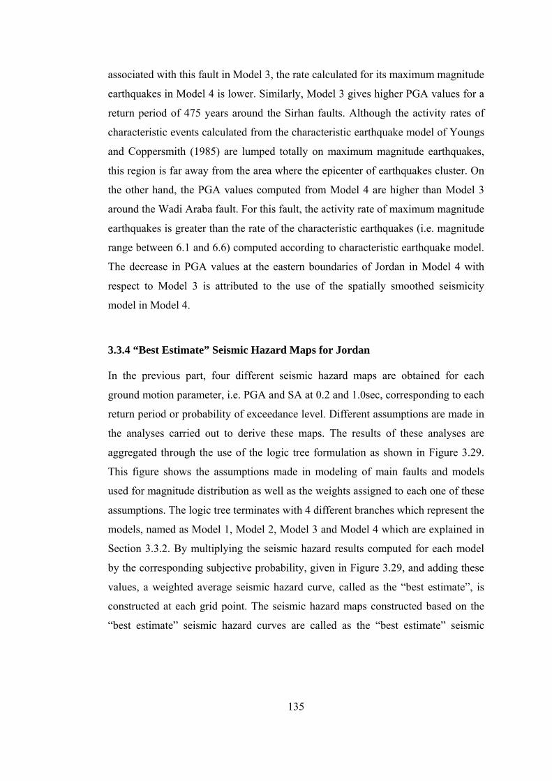
135
associated with this fault in Model 3, the rate calculated for its maximum magnitude
earthquakes in Model 4 is lower. Similarly, Model 3 gives higher PGA values for a
return period of 475 years around the Sirhan faults. Although the activity rates of
characteristic events calculated from the characteristic earthquake model of Youngs
and Coppersmith (1985) are lumped totally on maximum magnitude earthquakes,
this region is far away from the area where the epicenter of earthquakes cluster. On
the other hand, the PGA values computed from Model 4 are higher than Model 3
around the Wadi Araba fault. For this fault, the activity rate of maximum magnitude
earthquakes is greater than the rate of the characteristic earthquakes (i.e. magnitude
range between 6.1 and 6.6) computed according to characteristic earthquake model.
The decrease in PGA values at the eastern boundaries of Jordan in Model 4 with
respect to Model 3 is attributed to the use of the spatially smoothed seismicity
model in Model 4.
3.3.4 “Best Estimate” Seismic Hazard Maps for Jordan In the previous part, four different seismic hazard maps are obtained for each
ground motion parameter, i.e. PGA and SA at 0.2 and 1.0sec, corresponding to each
return period or probability of exceedance level. Different assumptions are made in
the analyses carried out to derive these maps. The results of these analyses are
aggregated through the use of the logic tree formulation as shown in Figure 3.29.
This figure shows the assumptions made in modeling of main faults and models
used for magnitude distribution as well as the weights assigned to each one of these
assumptions. The logic tree terminates with 4 different branches which represent the
models, named as Model 1, Model 2, Model 3 and Model 4 which are explained in
Section 3.3.2. By multiplying the seismic hazard results computed for each model
by the corresponding subjective probability, given in Figure 3.29, and adding these
values, a weighted average seismic hazard curve, called as the “best estimate”, is
constructed at each grid point. The seismic hazard maps constructed based on the
“best estimate” seismic hazard curves are called as the “best estimate” seismic

136
hazard maps. Figures 3.30 through 3.38 show the “best estimate” seismic hazard
maps derived in this study for Jordan.
Figure 3.29 Logic Tree Formulation for the Combinations of Different Assumptions (The values given in the parentheses are the subjective probabilities assigned to the corresponding assumptions.)
Area
Line
Exponential
Exponential
Characteristic
CEM(Y&C)
PCM
Modeling of the Main Faults Magnitude Distribution Combination
Model 1
Model 2
Model 3
Model 4
(0.5)
(0.5)
(0.5)
(0.5)
(0.5)
(0.5)
(0.5)
(0.25)
(0.125)
(0.125)

137
Figure 3.30 Best Estimate Seismic Hazard Map of Jordan for PGA (in g)
Corresponding to 10% Probability of Exceedance in 50 Years (475 Years Return Period)
Figure 3.31 Best Estimate Seismic Hazard Map of Jordan for PGA (in g)
Corresponding to 5% Probability of Exceedance in 50 Years (1000 Years Return Period)

138
Figure 3.32 Best Estimate Seismic Hazard Map of Jordan for PGA (in g)
Corresponding to 2% Probability of Exceedance in 50 Years (2475 Years Return Period)
Figure 3.33 Best Estimate Seismic Hazard Map of Jordan for SA at 0.2 sec (in g) Corresponding to 10% Probability of Exceedance in 50 Years (475 Years Return Period)

139
Figure 3.34 Best Estimate Seismic Hazard Map of Jordan for SA at 0.2 sec (in g)
Corresponding to 5% Probability of Exceedance in 50 Years (1000 Years Return Period)
Figure 3.35 Best Estimate Seismic Hazard Map of Jordan for SA at 0.2 sec (in g)
Corresponding to 2% Probability of Exceedance in 50 Years (2475 Years Return Period)

140
Figure 3.36 Best Estimate Seismic Hazard Map of Jordan for SA at 1.0 sec (in g) Corresponding to 10% Probability of Exceedance in 50 Years (475 Years Return Period)
Figure 3.37 Best Estimate Seismic Hazard Map of Jordan for SA at 1.0 sec (in g)
Corresponding to 5% Probability of Exceedance in 50 Years (1000 Years Return Period)
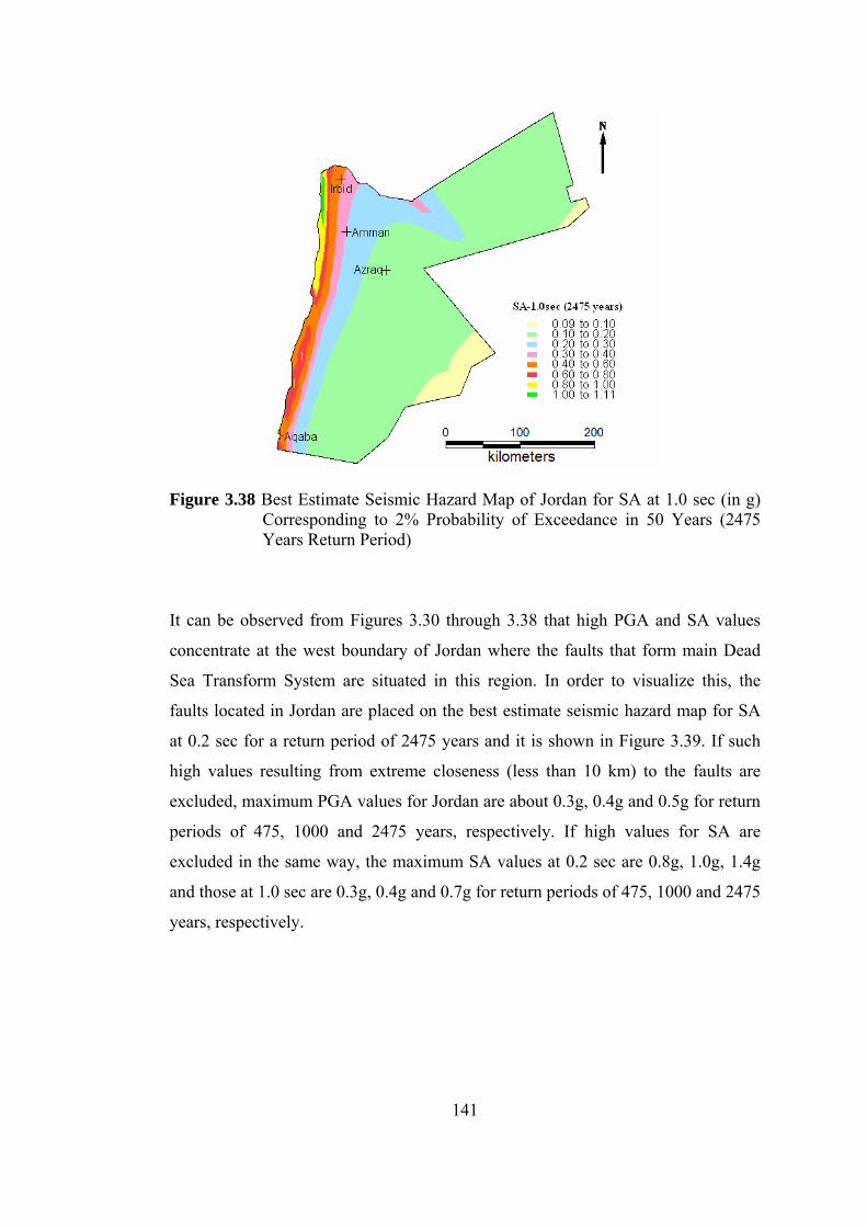
141
Figure 3.38 Best Estimate Seismic Hazard Map of Jordan for SA at 1.0 sec (in g)
Corresponding to 2% Probability of Exceedance in 50 Years (2475 Years Return Period)
It can be observed from Figures 3.30 through 3.38 that high PGA and SA values
concentrate at the west boundary of Jordan where the faults that form main Dead
Sea Transform System are situated in this region. In order to visualize this, the
faults located in Jordan are placed on the best estimate seismic hazard map for SA
at 0.2 sec for a return period of 2475 years and it is shown in Figure 3.39. If such
high values resulting from extreme closeness (less than 10 km) to the faults are
excluded, maximum PGA values for Jordan are about 0.3g, 0.4g and 0.5g for return
periods of 475, 1000 and 2475 years, respectively. If high values for SA are
excluded in the same way, the maximum SA values at 0.2 sec are 0.8g, 1.0g, 1.4g
and those at 1.0 sec are 0.3g, 0.4g and 0.7g for return periods of 475, 1000 and 2475
years, respectively.

142
Figure 3.39 Best Estimate Seismic Hazard Map of Jordan for SA at 0.2sec (in g)
Corresponding to 2% Probability of Exceedance in 50 Years (2475 Years Return Period) and Locations of Faults
Comparing the best estimate seismic hazard maps constructed in this study with the
corresponding maps derived by Jiménez (2004), it is observed that higher values are
obtained in this study. Jiménez (2004) applied area source modeling and
exponential magnitude distribution. Therefore, this difference is due to the
consideration of faults as line sources and the implementation of the characteristic
earthquake and maximum magnitude models in this study.
Yücemen (1992) derived a hazard map displaying the “Bayesian” estimate of
seismic hazard for PGA corresponding to 475 years return period and Al-Tarazi and
Sandvol (2007) obtained a seismic hazard map in terms of PGA with 10%
probability of exceedance in 50 years. These maps are given with the map
constructed in this study in Figure 3.40.

143
(a) (b)
(c)
Figure 3.40 Seismic Hazard Maps Derived for PGA with 10% Probability of
Exceedance in 50 Years by (a) Yücemen (1992) (Values are given in terms of %g) (b) Al-Tarazi and Sandvol (2007) (Values are given in terms of cm/sec2) (c) This study (Values are given in terms of g)

144
Compared with the studies carried out by Yücemen (1992) and Al-Tarazi and
Sandvol (2007), the PGA values given in this most recent study are slightly higher.
This difference can be attributed to the differences in seismic source modeling,
seismicity parameters assigned to them and attenuation relationships used in
computations as well as the use of more conservative models. It should be noted
that Yücemen (1992) used the attenuation equation proposed by Esteva and
Villaverde (1973) for peak ground acceleration whereas Al-Tarazi and Sandvol
(2007) used attenuation equations proposed by Boore et al. (1997), Sadigh et al.
(1997) and Campbell (1997) for peak ground acceleration at firm rock sites.
145
CHAPTER 4
CASE STUDY FOR A REGION: SEISMIC HAZARD MAPPING FOR THE BURSA PROVINCE
4.1 INTRODUCTION In the previous chapter, seismic hazard analysis is carried out for a large region
where a country, namely Jordan, is taken into consideration. Since the main
parameters of the faults were missing it was not possible to utilize the appropriate
models to assess the seismic hazard associated with faults. In this chapter, seismic
hazard analyses performed for a smaller region for which it was possible to collect
more detailed tectonic data. It is to be noted that the area of Bursa province (about
11000 km2) is almost nine times smaller than the area of Jordan (about 90000 km2).
The availability of the more detailed information on faults and fault segments
enables the implementation of more complex physical and stochastic models, such
as, segmentation and renewal in addition to the models applied in Chapter 3. This is
actually the most up-to-date trend in the development of new generation of seismic
hazard maps.
The Bursa province is selected as an example in order to illustrate the methodology
to be followed for this type of problems. Bursa is one of the most populated cities in
Turkey. Additionally, it is an important city for the industry in Turkey. Bursa is
located within a transitional zone of the extensional and contractional active
tectonic regimes (Yücemen at al., 2006). Therefore, it is seismically a very active
region. According to the current earthquake zoning map of Turkey, the portions of
this city are located in 1st and 2nd degree earthquake zones. Recent investigations on
the tectonics of the region and its near vicinity have resulted in better understanding
of active faults and estimation of their parameters. In view of this recent

146
information, seismic hazard for the Bursa province will be examined by applying
comprehensive source and earthquake occurrence models.
4.2 PREVIOUS PROBABILISTIC SEISMIC HAZARD ASSESSMENT
STUDIES FOR BURSA In literature, the studies focusing on the probabilistic estimation of seismic hazard
for the city of Bursa are quite limited in number. Accordingly, the seismic hazard
for this city is generally quantified based on current regulatory earthquake zoning
map of Turkey. This map was prepared by using the peak ground acceleration
(PGA) contour map that was constructed in the study of Gülkan et al. (1993) by
using probabilistic seismic hazard analyses methodology for a return period of 475
years. The earthquake zones in this map were determined based on the estimated
PGA values. The regions where PGA values are between 0.3g and 0.4g are
classified as the 2nd degree earthquake zone and those where PGA values are greater
than 0.4g are classified as the 1st degree earthquake zone.
Recently, Yücemen et al. (2006) carried out a probabilistic case study for the
assessment of seismic hazard of Bursa city center and its near vicinity. In this study,
41 fault segments were identified in the rectangular area bounded by 28˚- 30˚ E
longitudes and 39.75˚- 40.75˚N latitudes. Besides, five additional fault segments
were also considered in the North Marmara Fault zone. All of these faults were
modeled as line sources and they are assumed to produce only maximum
magnitude, characteristic earthquakes according to either Poisson or renewal
models. Therefore, maximum magnitude model was assumed as the magnitude
distribution in the study. They used a background area source with a truncated
exponential distribution in order to reflect the effects of earthquakes in the
magnitude range of 4.5-6.0 and assumed to be not related with any of the faults
identified. The seismicity parameters (i.e. ν and β) of the background area source
are estimated based on the earthquake catalog provided by the Earthquake Research
Department, General Directorate of Disaster Affairs. The epicentral distribution of
earthquakes in this catalog lies between 27.8˚- 30.2˚ E longitudes and 39˚- 41˚ N

147
latitudes. An alternative catalog was prepared by removing the secondary events
(i.e. fore- and after shocks) from this catalog. Also, incompleteness of these two
catalogs for small magnitude earthquakes was examined. Different seismicity
parameters were predicted from the combination of assumptions with respect to
incompleteness and dependence of secondary events. The PGA and spectral
accelerations (SA) at 0.2 sec and 1.0 sec were selected as ground motion
parameters. The empirical ground motion prediction equations given by Boore et al.
(1997) and Kalkan and Gülkan (2004) were used in their analyses. They performed
probabilistic seismic hazard analyses for each one of the combination of
assumptions and combined the results by the logic tree methodology. The results
were presented in the form of seismic hazard maps which show the distribution of
predicted PGA and SA values (T=0.2 sec and 1.0 sec) for return periods of 475 and
2475 years.
4.3 ASSESSMENT OF SEISMIC HAZARD FOR BURSA 4.3.1 Seismic Database and Seismic Sources 4.3.1.1 Seismic Database Earthquake catalogs are the most important sources of information used in seismic
hazard analysis since they describe the spatial and temporal distribution of past
earthquakes in the interested region. In order to assess seismic hazard for Bursa,
two seismic databases, namely ERD (Earthquake Research Department) and ISC
(International Seismological Centre), provided in the website of the Earthquake
Research Department in General Directorate of Disaster Affairs (ERD-GDDA,
2007) for the rectangular region between 26.0˚- 31.8˚ E longitudes and 38.8˚- 42.0˚
N latitudes are used. The ISC catalog contains the earthquakes that occurred
between years 1900 and 2002 while ERD catalog includes events occurred after
1991. In this study, the information given in ISC catalog is used for events occurred
until the end of year 2001 and since then the information given in ERD catalog is
taken into consideration. The earthquake catalog prepared in this way contains the

148
earthquakes that occurred in the region considered between 1901 and 2006. The
magnitudes of earthquakes in this catalog are given in different scales. They should
be converted to a common scale. In this study, moment magnitude scale, Mw, is
selected as the common magnitude scale.
Deniz (2006) developed the following conversion equations based on earthquakes
recorded in Turkey by using orthogonal regression:
14.6M25.2M bw −×= (4.1) 12.1M27.1M dw −×= (4.2) 66.2M57.1M Lw −×= (4.3) 81.2M54.0M Sw +×= (4.4) where, Mb: body wave magnitude, Md: duration magnitude, ML: local magnitude
and Ms: surface wave magnitude scales.
Ulusay et al. (2004), on the other hand, proposed the following conversion
equations derived by performing a simple linear regression analysis on the
earthquakes recorded in Turkey;
8994.0M2413.1M bw −×= (4.5) 4181.0M9495.0M dw +×= (4.6) 5921.1M7768.0M Lw +×= (4.7) 0402.2M6798.0M Sw +×= (4.8) The slope of the conversion equation estimated based on orthogonal regression is
greater than that obtained from the standard least squares regression. Accordingly,
moment magnitude values obtained from the conversion equations based on the
orthogonal regression will be larger compared to those based on the standard least
squares regression for large magnitude values. The opposite trend is valid for the
149
small magnitudes. Since the contribution of small magnitude earthquakes to seismic
hazard is considerably less than that of the large magnitude earthquakes, the use of
orthogonal regression based conversion equations will yield conservative seismic
hazard values. Except for Ms scale, compared with the conversion equations
developed by Ulusay et al. (2004), those proposed by Deniz (2006) underestimate
small magnitude earthquakes and overestimate large magnitude earthquakes.
In this study, the conversion equations developed by Deniz (2006) are applied to
achieve transformation of different magnitude scales to the Mw scale. In the
catalog, there are some earthquakes with magnitude values given in more than one
magnitude scale. For these earthquakes, the given magnitudes in different scales are
converted to the Mw magnitude scale and their average value, Mw-(ave), is taken as
the “best estimate” Mw value. The earthquakes with magnitudes, Mw, less than 4.5
are eliminated from the catalog. The resulting earthquake catalog includes 343
events and is given in Appendix D.
Secondary events should be removed from the earthquake catalog in order to fulfill
the underlying independence assumption of the Poisson distribution. This is
achieved by the method described in the previous chapter (see Section 3.3.1.1). It
should be noted that the earthquakes with magnitude equal to or greater than 6.0 are
assumed to be main shocks although they may be aftershock or foreshock of other
events. The resulting earthquake catalog includes 178 main shocks as given in
Appendix E.
Both earthquake catalogs are assumed to be complete for earthquakes with
magnitude greater than 5.0. However, the completeness is assumed to be valid since
1966 and 1967 for earthquakes with magnitudes between 4.5 and 5.0 in the catalogs
that include whole earthquakes and only main shocks, respectively.
Peak ground acceleration (PGA) and spectral accelerations (SA) at 0.2sec and 1.0
sec periods are selected as the basic parameters for the seismic hazard evaluation.
Taking into consideration the study conducted by Yücemen et al. (2006), the

150
attenuation relationships proposed by Boore et al. (1997) and Kalkan and Gülkan
(2004) are used to estimate seismic hazard in terms of this parameters. Since no
information is available about the site conditions all over Bursa, all seismic hazard
computations are carried out assuming for rock site condition.
4.3.1.2 Seismic Sources Bursa is under the seismic threat caused by several normal and strike-slip faults and
fault segments located in and near vicinity of Bursa. In the past, very destructive
historical earthquakes occurred in Bursa. These are: 28th February 1855 and 11th
April 1855 earthquakes with intensities of IX and X, respectively (Coburn and
Kuran, 1985; Ambraseys and Jackson, 2000) and 6th October 1964 Manyas
earthquake with Ms 7.0 (Erentöz and Kurtman, 1964) which caused the collapse or
heavy damage of buildings and many deaths.
In addition to the faults in Bursa, this city can be affected by the seismic activity
occurring in its vicinity. The North Anatolian Fault System (NAFS) is passing
though north of the city. Based on the renewal model, the probability of occurrence
of earthquakes with magnitude equal to or greater than 7.0 in the part of the NAFS
cutting across the floor of Marmara Sea was computed as 44±18 percent in the next
30 years (Parsons, 2004). Considering the fact that the 1970 Gediz earthquake with
magnitude 7.0 occurred at 250 km away from the Bursa caused heavy damage to
factories in the city (Yücemen et al., 2006), it is expected that an earthquake in the
Marmara Sea will also result in major damages to the structures located in Bursa.
Therefore, in addition to faults in and near vicinity of Bursa, main fault zones where
any seismic activity may affect the city are taken into consideration.
In this study, the faults within 26.0˚- 31.8˚ E longitudes and 38.8˚- 42.0˚ N and their
seismicity parameters are gathered from different sources available in the literature.
For the fault segments located between 28˚- 30˚ E longitudes and 39.75˚- 40.75˚N
latitudes, a comprehensive field investigation was carried out by Prof. Koçyiğit

151
(Yücemen et al., 2006). He identified forty one active fault segments in this region
and provided the information on type, average strike, average dip amount, length,
vertical and horizontal displacements, degree of activity, return period and the
maximum magnitude values, m1 (in Mw), for them. In addition, same type of
information for the fault segments of the two fault zones located outside of this
region; namely, Northern Marmara Fault Zone which is a part of the NAFS in the
Marmara Sea and Simav Fault Zone, was also presented. For the fault segments in
the 30˚-31˚ longitudes and 39.68˚-39.92˚ latitudes, the study carried out by Koçyiğit
(2005) for the delineation of active faults and assessment of the relevant parameters
of Eskişehir area is used. These segments are modeled based on the
recommendations of Koçyiğit (2006). The locations of fault segments in the part of
NAFS located east of İzmit Gulf are determined from Emre and Awata (2003),
Awata et al. (2003) and Şaroğlu et al. (1992) and Koçyiğit (2007). The remaining
main fault zones presented in Şaroğlu et al. (1992) are modeled as line sources.
While modeling these faults, Koçyiğit (2007) was consulted. In this study, all of
these faults and fault segments are examined in terms of the 91 segments as shown
in Figure 4.1. The distributions of earthquakes in the catalogs including all
earthquakes and only main shocks as well as the fault segments are shown in
Figures 4.2 and 4.3, respectively.
4.3.2 Methodology The seismic hazard in the region is assessed by combining the contributions of: (i)
earthquakes with magnitudes, M, between 4.5 and 6.0 that are not assigned to any
fault or fault segment and termed as “background seismic activity”, (ii) earthquakes
with magnitudes equal to or greater than 6.0 that may emanate from faults or fault
segments by rupturing the whole or a large portion of their lengths and release the
energy accumulated on them. The computation of seismic hazard due to these two
components will be explained in the following sections.

Figure 4.1 Map Showing the Locations of Faults (Thick Lines in Various Colors) Considered in This Study (Yücemen et al., 2006; Koçyiğit, 2005; Koçyiğit, 2006; Emre and Awata (2003), Awata et al., 2003; Şaroğlu et al., 1992; Koçyiğit, 2007)
27° 28° 29° 30° 31°
39°
40°
41°
42° 27° 28° 29° 30° 31°
39°
40°
41°
42° 26°
26°
152

153
26° 27° 28° 29° 30° 31°
26° 27° 28° 29° 30° 31°
39°
40°
41°
42°
39°
40°
41°
42°
Figure 4.2 Map Showing the Faults (Thick Black Lines) and the Spatial Distribution of All Earthquakes
26° 27° 28° 29° 30° 31°
26° 27° 28° 29° 30° 31°
39°
40°
41°
42°
39°
40°
41°
42°
Figure 4.3 Map Showing the Faults (Thick Black Lines) and the Spatial Distribution of Main Shocks

154
4.3.2.1 Seismic Hazard Resulting From Background Seismic Activity In order to quantify the seismic hazard due to background seismic activity, the
information given for earthquakes within the range of 4.5 ≤ M ≤ 6.0 in the two
earthquake catalogs that include whole events and only main shocks are used. As
explained in Section 4.3.1.1, the catalogs including the whole earthquakes and only
the main shocks are assumed to be complete for events with M ≥ 5.0 and for those
with 4.5 ≤ M < 5.0 since 1966 and 1967, respectively. For background seismic
activity, four different values are computed for the slope of Gutenberg Richter
magnitude recurrence relationships, ⏐b⏐, β=b×ln 10 and for the annual activity rate,
ν, by considering the alternative assumptions on completeness and elimination of
secondary events as outlined in Table 4.1. In the cases where the catalog data are
corrected for completeness, the range of magnitudes between 4.5 and 6.0 are
divided into bins. Then, the number of earthquakes having magnitude between the
bounds of each magnitude bin are counted and divided by the period where the data
is complete to calculate the corresponding artificially completed annual activity
rates, νi. Afterwards, the ν and ⏐b⏐values are calculated based on the νi values.
Table 4.1 b, β and ν Values Computed According to Alternative Assumptions for
the Background Seismic Activity
Catalog Type Correction for Incompleteness ⏐b⏐ ⏐β⏐ ν No 0.99 2.285 2.972
All Earthquakes Yes 1.08 2.491 4.213No 0.81 1.869 1.415
Only Main Shocks Yes 0.88 2.037 1.944 Contribution of background events to seismic hazard is calculated by using two
different models; spatially smoothed seismicity model of Frankel (1995) and
background area source with uniform seismicity. Seismic hazard computations for
background area source with uniform seismicity are carried out by using EZ-FRISK
155
(Risk Engineering, 2005). On the other hand, in the calculation of the contribution
of background seismic activity based on the spatially smoothed seismicity model of
Frankel (1995), the computer programs developed at USGS (Frankel et al., 1996)
and later modified by Kalkan (2007) in order to include additional attenuation
relationships are utilized. Analyses are carried out by using combinations of
different assumptions with respect to incompleteness of earthquake catalogs and
dependence of events in them (i.e., inclusion of secondary events or not). In the
analyses carried out by using background source, an area source bounded by 26.0˚-
31.8˚ E longitudes and 38.8˚- 42.0˚ N latitudes is defined. For this source, truncated
exponential magnitude distribution with different β and ν values presented in Table
4.1 is used in the analyses. The lower and upper bounds of this distribution are
assigned as 4.5 and 6.0, respectively. Six different seismic hazard analyses are
carried out by using spatially smoothed seismicity model of Frankel (1995) based
on the same combinations of assumptions. The correlation distance for smoothing is
assumed to be 50 km in all cases. In the analyses in which the completeness in the
catalogs are not taken into consideration, the earthquakes with 4.5 ≤ M ≤ 6.0 in the
two earthquake catalogs that includes whole events and only main shocks are used.
In order to adjust for incompleteness, seismic hazard analyses are carried out by
using earthquakes with 5.0 ≤ M ≤ 6.0 occurred since 1901; and those with 4.5 ≤ M
≤ 6.0 since 1966 and 1967 in the catalogs including all events and only main
shocks, respectively. Then, the results of analyses based on the same catalog are
combined by giving equal weights to each one of the assumptions. Figure 4.4
describes schematically the different combinations considered and the methodology
followed in these analyses. First, seismic hazard analyses are performed to obtain the hazard curves for a
selected site (40.24o N, 29.08o E) which approximately corresponds to the city
center of Bursa. Figure 4.5 shows the seismic hazard curves obtained by using
attenuation relationships proposed by Kalkan and Gülkan (2004) and Boore et al.
(1997) for peak ground acceleration (PGA) at rock sites ( shear wave velocity, Vs, is
assumed to be equal to 700 m/s). From the comparison of seismic hazard curves

156
given in Figure 4.5 (i) with those in Figure 4.5 (ii), it can be observed that the
influence of utilizing the attenuation models proposed by Kalkan and Gülkan
(2004) and Boore et al. (1997) is insignificant at small PGA values but it becomes
apparent at larger PGA values.
In order to illustrate the spatial sensitivity of seismic hazard results to the seismicity
models and different assumptions, seismic hazard analyses are carried out at all grid
points with a spacing of 0.02°×0.02° in latitude and longitude in the region bounded
by 26.0˚- 31.8˚ E longitudes and 38.8˚- 42.0˚ N latitudes and seismic hazard maps
for PGA corresponding to return periods of 475, 1000 and 2475 years are
constructed. In the analyses, equal weights are given to both attenuation
relationships. Figure 4.6 through Figure 4.11 show seismic hazard maps obtained by
using spatially smoothed seismicity model.
As explained in Chapter 3, almost a uniform seismic hazard distribution is obtained
for the selected ground motion parameter from the seismic hazard analyses carried
out by using a background area source with uniform seismicity. The maximum
PGA values obtained from the analyses carried out by using the background area
source with uniform seismicity are presented in Table 4.2 for return periods of 475,
1000, and 2475 years.
Table 4.2 Maximum PGA Values (in g) Obtained from Background Area Source
with Uniform Seismicity
Return Period (Year)
Catalog Type Correction for Incompleteness
475 1000 2475 No 0.18 0.22 0.29 All Earthquakes Yes 0.19 0.24 0.31 No 0.14 0.19 0.24 Only Main Shocks Yes 0.16 0.20 0.26

157

158
0.00001
0.0001
0.001
0.01
0.1
1
10
0.01 0.1 1
PGA(g)
Ann
ual F
requ
ancy
of E
xcee
danc
e (a)(b)(c)(d)(e)(f)(g)(h)
(i) Boore et al. (1997)
0.00001
0.0001
0.001
0.01
0.1
1
10
0.01 0.1 1
PGA(g)
Ann
ual F
requ
ency
of E
xcee
danc
e (a)(b)(c)(d)(e)(f)(g)(h)
(ii) Kalkan and Gülkan (2004)
Figure 4.5 Seismic Hazard Curves Obtained by Using Spatially Smoothed Seismicity Model with; (a) Main Shocks in the Incomplete Database, (b) All Earthquakes in the Incomplete Database (c) Main Shocks and Adjusting for Incompleteness, (d) All Earthquakes and Adjusting for Incompleteness and by Using Uniform Seismicity with; (e) Main Shocks in the Incomplete Database, (f) All Earthquakes in the Incomplete Database, (g) Main Shocks and Adjusting for Incompleteness, (h) All Earthquakes and Adjusting for Incompleteness

159
26° 27° 28° 29° 30° 31°
26° 27° 28° 29° 30° 31°
39°
40°
41°
42°
39°
40°
41°
42°
(a)
26° 27° 28° 29° 30° 31°
26° 27° 28° 29° 30° 31°
39°
40°
41°
42°
39°
40°
41°
42°
(b)
Figure 4.6 Seismic Hazard Maps for PGA (in g) Corresponding to the Return Period of 475 Years Obtained by Using Spatially Smoothed Seismicity Model with Main Shocks (a) Incomplete Database (b) Database Adjusted for Incompleteness

160
26° 27° 28° 29° 30° 31°
26° 27° 28° 29° 30° 31°
39°
40°
41°
42°
39°
40°
41°
42°
(a)
26° 27° 28° 29° 30° 31°
26° 27° 28° 29° 30° 31°
39°
40°
41°
42°
39°
40°
41°
42°
(b)
Figure 4.7 Seismic Hazard Maps for PGA (in g) Corresponding to the Return Period of 475 Years Obtained by Using Spatially Smoothed Seismicity Model with All Earthquakes (a) Incomplete Database (b) Database Adjusted for Incompleteness

161
26° 27° 28° 29° 30° 31°
26° 27° 28° 29° 30° 31°
39°
40°
41°
42°
39°
40°
41°
42°
(a)
26° 27° 28° 29° 30° 31°
26° 27° 28° 29° 30° 31°
39°
40°
41°
42°
39°
40°
41°
42°
(b)
Figure 4.8 Seismic Hazard Maps for PGA (in g) Corresponding to the Return Period of 1000 years Obtained by Using Spatially Smoothed Seismicity Model with Main Shocks (a) Incomplete Database (b) Database Adjusted for Incompleteness

162
26° 27° 28° 29° 30° 31°
26° 27° 28° 29° 30° 31°
39°
40°
41°
42°
39°
40°
41°
42°
(a)
26° 27° 28° 29° 30° 31°
26° 27° 28° 29° 30° 31°
39°
40°
41°
42°
39°
40°
41°
42°
(b)
Figure 4.9 Seismic Hazard Maps for PGA (in g) Corresponding to the Return Period of 1000 years Obtained by Using Spatially Smoothed Seismicity Model with All Earthquakes (a) Incomplete Database (b) Database Adjusted for Incompleteness

163
26° 27° 28° 29° 30° 31°
26° 27° 28° 29° 30° 31°
39°
40°
41°
42°
39°
40°
41°
42°
(a)
26° 27° 28° 29° 30° 31°
26° 27° 28° 29° 30° 31°
39°
40°
41°
42°
39°
40°
41°
42°
(b)
Figure 4.10 Seismic Hazard Maps for PGA (in g) Corresponding to the Return Period of 2475 years Obtained by Using Spatially Smoothed Seismicity Model with Main Shocks (a) Incomplete Database (b) Database Adjusted for Incompleteness

164
26° 27° 28° 29° 30° 31°
26° 27° 28° 29° 30° 31°
39°
40°
41°
42°
39°
40°
41°
42°
(a)
26° 27° 28° 29° 30° 31°
26° 27° 28° 29° 30° 31°
39°
40°
41°
42°
39°
40°
41°
42°
(b)
Figure 4.11 Seismic Hazard Maps for PGA (in g) Corresponding to the Return Period of 2475 years Obtained by Using Spatially Smoothed Seismicity Model with All Earthquakes (a) Incomplete Database (b) Database Adjusted for Incompleteness
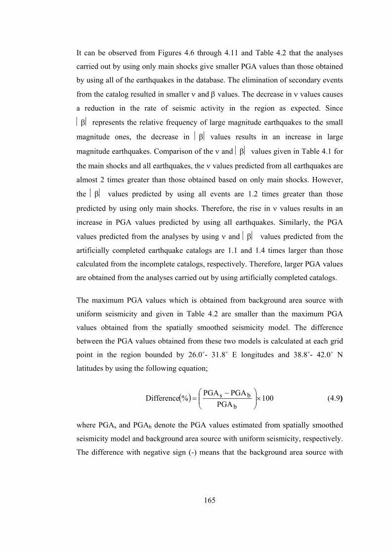
165
It can be observed from Figures 4.6 through 4.11 and Table 4.2 that the analyses
carried out by using only main shocks give smaller PGA values than those obtained
by using all of the earthquakes in the database. The elimination of secondary events
from the catalog resulted in smaller ν and β values. The decrease in ν values causes
a reduction in the rate of seismic activity in the region as expected. Since
⏐β⏐ represents the relative frequency of large magnitude earthquakes to the small
magnitude ones, the decrease in ⏐β⏐ values results in an increase in large
magnitude earthquakes. Comparison of the ν and ⏐β⏐ values given in Table 4.1 for
the main shocks and all earthquakes, the ν values predicted from all earthquakes are
almost 2 times greater than those obtained based on only main shocks. However,
the ⏐β⏐ values predicted by using all events are 1.2 times greater than those
predicted by using only main shocks. Therefore, the rise in ν values results in an
increase in PGA values predicted by using all earthquakes. Similarly, the PGA
values predicted from the analyses by using ν and ⏐β⏐ values predicted from the
artificially completed earthquake catalogs are 1.1 and 1.4 times larger than those
calculated from the incomplete catalogs, respectively. Therefore, larger PGA values
are obtained from the analyses carried out by using artificially completed catalogs.
The maximum PGA values which is obtained from background area source with
uniform seismicity and given in Table 4.2 are smaller than the maximum PGA
values obtained from the spatially smoothed seismicity model. The difference
between the PGA values obtained from these two models is calculated at each grid
point in the region bounded by 26.0˚- 31.8˚ E longitudes and 38.8˚- 42.0˚ N
latitudes by using the following equation;
( ) 100PGA
PGAPGA%Difference
b
bs ×⎟⎟⎠
⎞⎜⎜⎝
⎛ −= (4.9)
where PGAs and PGAb denote the PGA values estimated from spatially smoothed
seismicity model and background area source with uniform seismicity, respectively.
The difference with negative sign (-) means that the background area source with

166
uniform seismicity gives higher PGA values than the spatially smoothed seismicity
model and the difference with positive sign represents the opposite case.
Figures 4.12 through 4.23 show the spatial variation of differences in PGA values
obtained from the spatially smoothed seismicity model and the background area
source with uniform seismicity according to different combinations of assumptions
on earthquakes in the catalogs with respect to completeness and dependence. In
these figures, it can be observed that spatially smoothed seismicity model gives
higher PGA values than the background area source with uniform seismicity (i.e.
positive difference values) especially at the regions where the epicenters of
earthquakes become dense. On the other hand, negative differences (i.e. background
area source gives higher PGA values than spatially smoothed seismicity model) are
observed especially at the regions where the epicenters of earthquakes are scarce or
no earthquakes occurred at the past. For the Bursa province in which the seismic
hazard is under consideration for this study, positive differences is observed at
southwestern part whereas negative one is seen at the northeastern part for the cases
in which main shocks are used in the analyses. For the cases in which all
earthquakes are considered, the positive differences are observed at the middle part
of the Bursa province and extend through northeastern and southwestern parts. The
maximum difference observed from all cases for Bursa province is less than 25%.
This means that modeling background seismic activity with background area source
model or spatially smoothed seismicity model has minor effect on the final results.

167
26° 27° 28° 29° 30° 31°
26° 27° 28° 29° 30° 31°
39°
40°
41°
42°
39°
40°
41°
42°
Figure 4.12 Map Showing the Spatial Variation of the Difference between the PGA
Values Obtained from Spatially Smoothed Seismicity Model and Background Area Source with Main Shocks and Incomplete Database for a Return Period of 475 Years
26° 27° 28° 29° 30° 31°
26° 27° 28° 29° 30° 31°
39°
40°
41°
42°
39°
40°
41°
42°
Figure 4.13 Map Showing the Spatial Variation of the Difference between the PGA Values Obtained from Spatially Smoothed Seismicity Model and Background Area Source with Main Shocks and Incomplete Database for a Return Period of 2475 Years
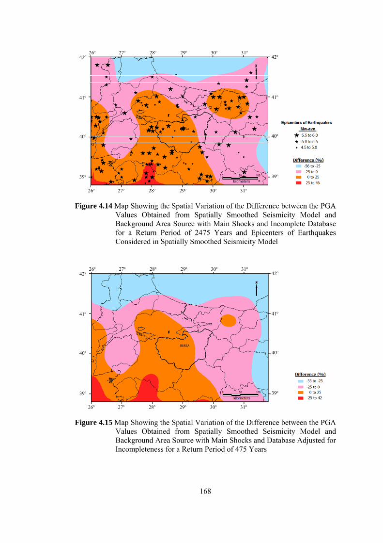
168
26° 27° 28° 29° 30° 31°
26° 27° 28° 29° 30° 31°
39°
40°
41°
42°
39°
40°
41°
42°
Figure 4.14 Map Showing the Spatial Variation of the Difference between the PGA
Values Obtained from Spatially Smoothed Seismicity Model and Background Area Source with Main Shocks and Incomplete Database for a Return Period of 2475 Years and Epicenters of Earthquakes Considered in Spatially Smoothed Seismicity Model
26° 27° 28° 29° 30° 31°
26° 27° 28° 29° 30° 31°
39°
40°
41°
42°
39°
40°
41°
42°
Figure 4.15 Map Showing the Spatial Variation of the Difference between the PGA
Values Obtained from Spatially Smoothed Seismicity Model and Background Area Source with Main Shocks and Database Adjusted for Incompleteness for a Return Period of 475 Years
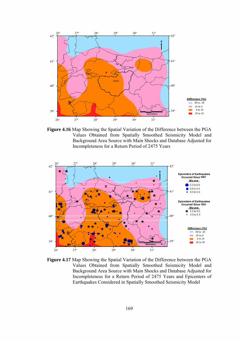
169
26° 27° 28° 29° 30° 31°
26° 27° 28° 29° 30° 31°
39°
40°
41°
42°
39°
40°
41°
42°
Figure 4.16 Map Showing the Spatial Variation of the Difference between the PGA
Values Obtained from Spatially Smoothed Seismicity Model and Background Area Source with Main Shocks and Database Adjusted for Incompleteness for a Return Period of 2475 Years
26° 27° 28° 29° 30° 31°
26° 27° 28° 29° 30° 31°
39°
40°
41°
42°
39°
40°
41°
42°
Figure 4.17 Map Showing the Spatial Variation of the Difference between the PGA
Values Obtained from Spatially Smoothed Seismicity Model and Background Area Source with Main Shocks and Database Adjusted for Incompleteness for a Return Period of 2475 Years and Epicenters of Earthquakes Considered in Spatially Smoothed Seismicity Model

170
26° 27° 28° 29° 30° 31°
26° 27° 28° 29° 30° 31°
39°
40°
41°
42°
39°
40°
41°
42°
Figure 4.18 Map Showing the Spatial Variation of the Difference between the PGA
Values Obtained from Spatially Smoothed Seismicity Model and Background Area Source with All Earthquakes and Incomplete Database for a Return Period of 475 Years
26° 27° 28° 29° 30° 31°
26° 27° 28° 29° 30° 31°
39°
40°
41°
42°
39°
40°
41°
42°
Figure 4.19 Map Showing the Spatial Variation of the Difference between the PGA
Values Obtained from Spatially Smoothed Seismicity Model and Background Area Source with All Earthquakes and Incomplete Database for a Return Period of 2475 Years

171
26° 27° 28° 29° 30° 31°
26° 27° 28° 29° 30° 31°
39°
40°
41°
42°
39°
40°
41°
42°
Figure 4.20 Map Showing the Spatial Variation of the Difference between the PGA
Values Obtained from Spatially Smoothed Seismicity Model and Background Area Source with All Earthquakes and Incomplete Database for a Return Period of 2475 Years and Epicenters of Earthquakes Considered in Spatially Smoothed Seismicity Model
26° 27° 28° 29° 30° 31°
26° 27° 28° 29° 30° 31°
39°
40°
41°
42°
39°
40°
41°
42°
Figure 4.21 Map Showing the Spatial Variation of the Difference between the PGA
Values Obtained from Spatially Smoothed Seismicity Model and Background Area Source with All Earthquakes and Database Adjusted for Incompleteness for a Return Period of 475 Years
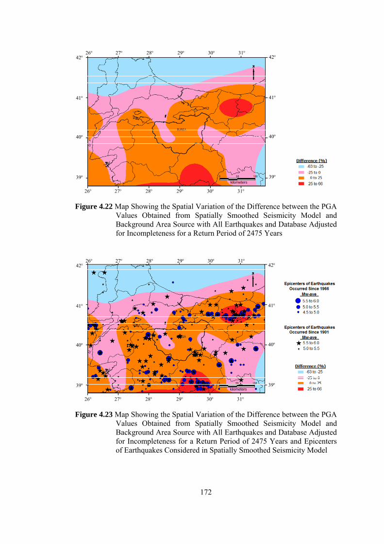
172
26° 27° 28° 29° 30° 31°
26° 27° 28° 29° 30° 31°
39°
40°
41°
42°
39°
40°
41°
42°
Figure 4.22 Map Showing the Spatial Variation of the Difference between the PGA
Values Obtained from Spatially Smoothed Seismicity Model and Background Area Source with All Earthquakes and Database Adjusted for Incompleteness for a Return Period of 2475 Years
26° 27° 28° 29° 30° 31°
26° 27° 28° 29° 30° 31°
39°
40°
41°
42°
39°
40°
41°
42°
Figure 4.23 Map Showing the Spatial Variation of the Difference between the PGA
Values Obtained from Spatially Smoothed Seismicity Model and Background Area Source with All Earthquakes and Database Adjusted for Incompleteness for a Return Period of 2475 Years and Epicenters of Earthquakes Considered in Spatially Smoothed Seismicity Model

173
4.3.2.2 Seismic Hazard Resulting From Faults As explained above, the contributions of earthquakes with magnitude equal to or
greater than 6.0 are calculated by attributing the related seismic activity to the faults
and fault segments shown in Figure 4.1. It is assumed that energy along these faults
and fault segments are released by characteristic events that rupture the whole or a
large portion of the length of the fault. Consequently, the maximum magnitude
earthquakes that the fault segments may generate and their return periods are the
main parameters in these calculations.
For the fault segments that are delineated based on the study of Yücemen et al.
(2006), the maximum magnitude values and their return periods given in this
reference are used. For those fault segments identified based on Koçyiğit (2005),
only maximum magnitude values are given in his study. For the rest of the fault
segments, their maximum magnitudes are assigned based on their lengths by using
the equation proposed by Wells and Coppersmith (1994) which is given below:
)SRLlog(16.108.5Mw += (4.10) where; M is the earthquake magnitude, SRL is the surface rupture length. In this
study, SRL is assumed to be equal to the fault length. However, the lengths of
longest segments of faults; numbered as F2, F3, F7, F8 and F9 where F stands for
fault, are used in the determination of their maximum magnitude earthquakes. For
the return periods of the maximum magnitudes of all fault segments, except those
given in Yücemen et al. (2006), Koçyiğit (2007) is consulted. Table 4.3 shows the
parameters of fault segments considered in this study.
In order to predict probabilities of future occurrences of maximum magnitude,
characteristic earthquakes along these fault segments, both the memoryless Poisson
and the time dependent renewal models are utilized. In the Poisson model, the
annual rate of characteristic earthquakes for each segment is taken as the reciprocal
of the lower bound of its return period given in Table 4.3. Therefore, conservative
estimates of annual activity rates are used in the seismic hazard computations.
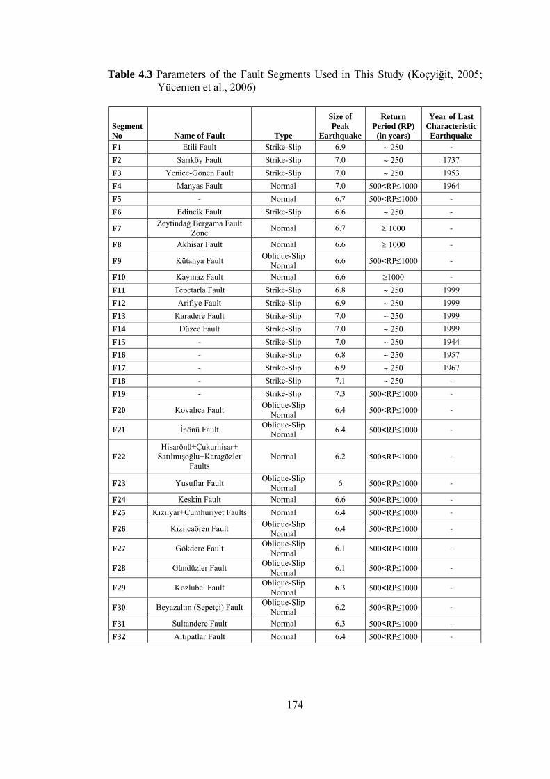
174
Table 4.3 Parameters of the Fault Segments Used in This Study (Koçyiğit, 2005; Yücemen et al., 2006)
Segment No Name of Fault Type
Size of Peak
Earthquake
Return Period (RP)
(in years)
Year of Last Characteristic
Earthquake F1 Etili Fault Strike-Slip 6.9 ∼ 250 -
F2 Sarıköy Fault Strike-Slip 7.0 ∼ 250 1737 F3 Yenice-Gönen Fault Strike-Slip 7.0 ∼ 250 1953 F4 Manyas Fault Normal 7.0 500<RP≤1000 1964 F5 - Normal 6.7 500<RP≤1000 - F6 Edincik Fault Strike-Slip 6.6 ∼ 250 -
F7 Zeytindağ Bergama Fault Zone Normal 6.7 ≥ 1000 -
F8 Akhisar Fault Normal 6.6 ≥ 1000 -
F9 Kütahya Fault Oblique-Slip Normal 6.6 500<RP≤1000 -
F10 Kaymaz Fault Normal 6.6 ≥1000 - F11 Tepetarla Fault Strike-Slip 6.8 ∼ 250 1999 F12 Arifiye Fault Strike-Slip 6.9 ∼ 250 1999 F13 Karadere Fault Strike-Slip 7.0 ∼ 250 1999 F14 Düzce Fault Strike-Slip 7.0 ∼ 250 1999 F15 - Strike-Slip 7.0 ∼ 250 1944 F16 - Strike-Slip 6.8 ∼ 250 1957 F17 - Strike-Slip 6.9 ∼ 250 1967 F18 - Strike-Slip 7.1 ∼ 250 -
F19 - Strike-Slip 7.3 500<RP≤1000 -
F20 Kovalıca Fault Oblique-Slip Normal 6.4 500<RP≤1000 -
F21 İnönü Fault Oblique-Slip Normal 6.4 500<RP≤1000 -
F22 Hisarönü+Çukurhisar+
Satılmışoğlu+Karagözler Faults
Normal 6.2 500<RP≤1000 -
F23 Yusuflar Fault Oblique-Slip Normal 6 500<RP≤1000 -
F24 Keskin Fault Normal 6.6 500<RP≤1000 -
F25 Kızılyar+Cumhuriyet Faults Normal 6.4 500<RP≤1000 -
F26 Kızılcaören Fault Oblique-Slip Normal 6.4 500<RP≤1000 -
F27 Gökdere Fault Oblique-Slip Normal 6.1 500<RP≤1000 -
F28 Gündüzler Fault Oblique-Slip Normal 6.1 500<RP≤1000 -
F29 Kozlubel Fault Oblique-Slip Normal 6.3 500<RP≤1000 -
F30 Beyazaltın (Sepetçi) Fault Oblique-Slip Normal 6.2 500<RP≤1000 -
F31 Sultandere Fault Normal 6.3 500<RP≤1000 -
F32 Altıpatlar Fault Normal 6.4 500<RP≤1000 -

175
Table 4.3 (Continued) Parameters of the Fault Segments Used in This Study (Koçyiğit, 2005; Yücemen et al., 2006)
Segment No Name of Fault Type
Size of Peak
Earthquake
Return Period (RP)
(in years)
Year of Last Characteristic
Earthquake F33 Karacaören Fault Normal 6.5 500<RP≤1000 -
F34 Gülpınar Fault Oblique-Slip Normal 6.3 ≥ 1000 -
F35 Meşelik Fault Oblique-Slip Normal 6.1 ≥ 1000 -
F36 Esmekaya+Soğucak+
Karaözkuyu+Kavacık+ Eğriöz+Kozkaya Faults
Oblique-Slip Normal 6.7 500<RP≤1000 1956
F37 Uçmakdere+Ganos Fault Strike-Slip 7.2 283 1912 F38 Kumbağı Fault Strike-Slip 7 283 1912
F39 Central Fault Strike-Slip 6.4 500<RP≤1000 1556
F40 Kumburgaz Fault Strike-Slip 6.5 257±23 1766
F41 Yeşilköy Fault Strike-Slip 7 257±23 1766
F42 Adalar Fault Normal 6.9 200<RP≤500 1766
F43 Darıca Fault Strike-Slip 6.5 500<RP≤1000 1894
F44 Agaçlı Fault Normal 6.8 ≥ 1000 -
F45 Muratdağı Fault Normal 7 ≥ 1000 1970
F46 Erdoğmuş Fault Normal 6.8 ≥ 1000 1970 F47 Abide Fault Normal 6.5 ≥ 1000 -
F48 Simav Fault Normal 7.2 ≥ 1000 -
F49 Bursa Fault Oblique-Slip Normal 7.2 ≥ 1000 1855
F50 Sayfiye Fault Oblique-Slip Normal 6.8 ≥ 1000 -
F51 Alaçam Fault Oblique-Slip Normal 6.7 500<RP≤1000 -
F52 Soğukpınar Fault Oblique-Slip Normal 6.7 ≥ 1000 -
F53 Çalı Fault Oblique-Slip Normal 6.8 ≥ 1000 1855
F54 Ayaz Fault Oblique-Slip Normal 6.4 ≥ 1000 1855
F55 M. Kemalpaşa Fault Oblique-Slip Normal 6.5 ≥ 1000 1964
F56 Derecik Fault Oblique-Slip Normal 6.5 ≥ 1000 1964
F57 Yeniköy Fault Oblique-Slip Normal 6.2 ≥ 1000 1964
F58 Çavuşköy Fault Oblique-Slip Normal 6 ≥ 1000 -
F59 Kestel Fault Set Oblique-Slip Normal 6.4 ≥ 1000 -
F60 Taşlık Fault Oblique-Slip Normal 6 ≥ 1000 -
F61 Demirtaş Fault Oblique-Slip Normal 6.6 ≥ 1000 -

176
Table 4.3 (Continued) Parameters of the Fault Segments Used in This Study (Koçyiğit, 2005; Yücemen et al., 2006)
Segment No Name of Fault Type
Size of Peak
Earthquake
Return Period (RP)
(in years)
Year of Last Characteristic Earthquake
F62 Karahıdır Fault Oblique-Slip Normal 6.7 ≥ 1000 -
F63 Eymir Fault Oblique-Slip Normal 6.6 ≥ 1000 -
F64 Boğazköy Fault Oblique-Slip Normal 6.7 ≥ 1000 -
F65 Eskiköy Fault Oblique-Slip Normal 6.9 ≥ 1000 -
F66 Kozpınar Fault Oblique-Slip Normal 7 ≥ 1000 -
F67 Erikli Fault Oblique-Slip Normal 6.9 ≥ 1000 -
F68 Dodurga Fault Oblique-Slip Normal 6.2 ≥ 1000 -
F69 Gemlik Fault Strike-Slip 6.4 500<RP≤1000 - F70 Gürle Fault Strike-Slip 6.3 500<RP≤1000 - F71 Gençali Fault Strike-Slip 6.3 500<RP≤1000 - F72 Altıntaş-Kurşunlu Fault Strike-Slip 6.2 500<RP≤1000 - F73 Narlıca Fault Strike-Slip 6.2 500<RP≤1000 - F74 Şükrüye Fault Strike-Slip 6.5 500<RP≤1000 - F75 Çamdibi Fault Strike-Slip 7 ≥ 1000 - F76 Karadin Fault Strike-Slip 6.5 500<RP≤1000 - F77 Orhaniye Fault Strike-Slip 6.5 500<RP≤1000 -
F78 Kurtköy-Gökçedere Fault Oblique-Slip Normal 6.4 500<RP≤1000 -
F79 Koyunhisar Fault Strike-Slip 6.5 500<RP≤1000 - F80 Kavaklı Fault Strike-Slip 6.3 500<RP≤1000 - F81 Mudanya Fault Strike-Slip 6.5 500<RP≤1000 - F82 Boğazköy-Ekinli Fault Strike-Slip 6.7 500<RP≤1000 - F83 Kurşunlu Fault Strike-Slip 6.6 500<RP≤1000 - F84 Karamürsel Fault Strike-Slip 6.7 250-300 1999 F85 Çınarcık Fault Strike-Slip 6.9 ≥ 400 - F86 Laledere Fault Strike-Slip 6.5 500<RP≤1000 - F87 Gölcük Fault Strike-Slip 6.7 210-280 1999 F88 Körfez Fault Strike-Slip 6.4 250-300 1999 F89 Ortaca Fault Normal 6.3 ≥ 1000 - F90 Akçabük Fault Normal 6.5 ≥ 1000 - F91 Bandırma Fault Strike-Slip 7 ≥ 1000 -
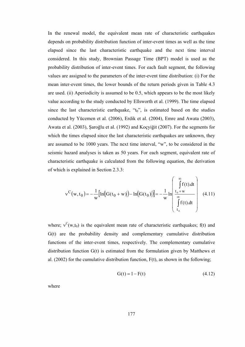
177
In the renewal model, the equivalent mean rate of characteristic earthquakes
depends on probability distribution function of inter-event times as well as the time
elapsed since the last characteristic earthquake and the next time interval
considered. In this study, Brownian Passage Time (BPT) model is used as the
probability distribution of inter-event times. For each fault segment, the following
values are assigned to the parameters of the inter-event time distribution: (i) For the
mean inter-event times, the lower bounds of the return periods given in Table 4.3
are used. (ii) Aperiodicity is assumed to be 0.5, which appears to be the most likely
value according to the study conducted by Ellsworth et al. (1999). The time elapsed
since the last characteristic earthquake, “t0”, is estimated based on the studies
conducted by Yücemen et al. (2006), Erdik et al. (2004), Emre and Awata (2003),
Awata et al. (2003), Şaroğlu et al. (1992) and Koçyiğit (2007). For the segments for
which the times elapsed since the last characteristic earthquakes are unknown, they
are assumed to be 1000 years. The next time interval, “w”, to be considered in the
seismic hazard analyses is taken as 50 years. For each segment, equivalent rate of
characteristic earthquake is calculated from the following equation, the derivation
of which is explained in Section 2.3.3:
( ) ( ) ( )[ ]
⎟⎟⎟⎟⎟⎟
⎠
⎞
⎜⎜⎜⎜⎜⎜
⎝
⎛
−=−+−=ν
∫
∫∞
∞
+
0
0
t
wt000
C
dt).t(f
dt).t(f
lnw1)t(Gln)wt(Gln
w1t,w (4.11)
where; νC(w,t0) is the equivalent mean rate of characteristic earthquakes; f(t) and
G(t) are the probability density and complementary cumulative distribution
functions of the inter-event times, respectively. The complementary cumulative
distribution function G(t) is estimated from the formulation given by Matthews et
al. (2002) for the cumulative distribution function, F(t), as shown in the following;
)t(F1)t(G −= (4.12) where
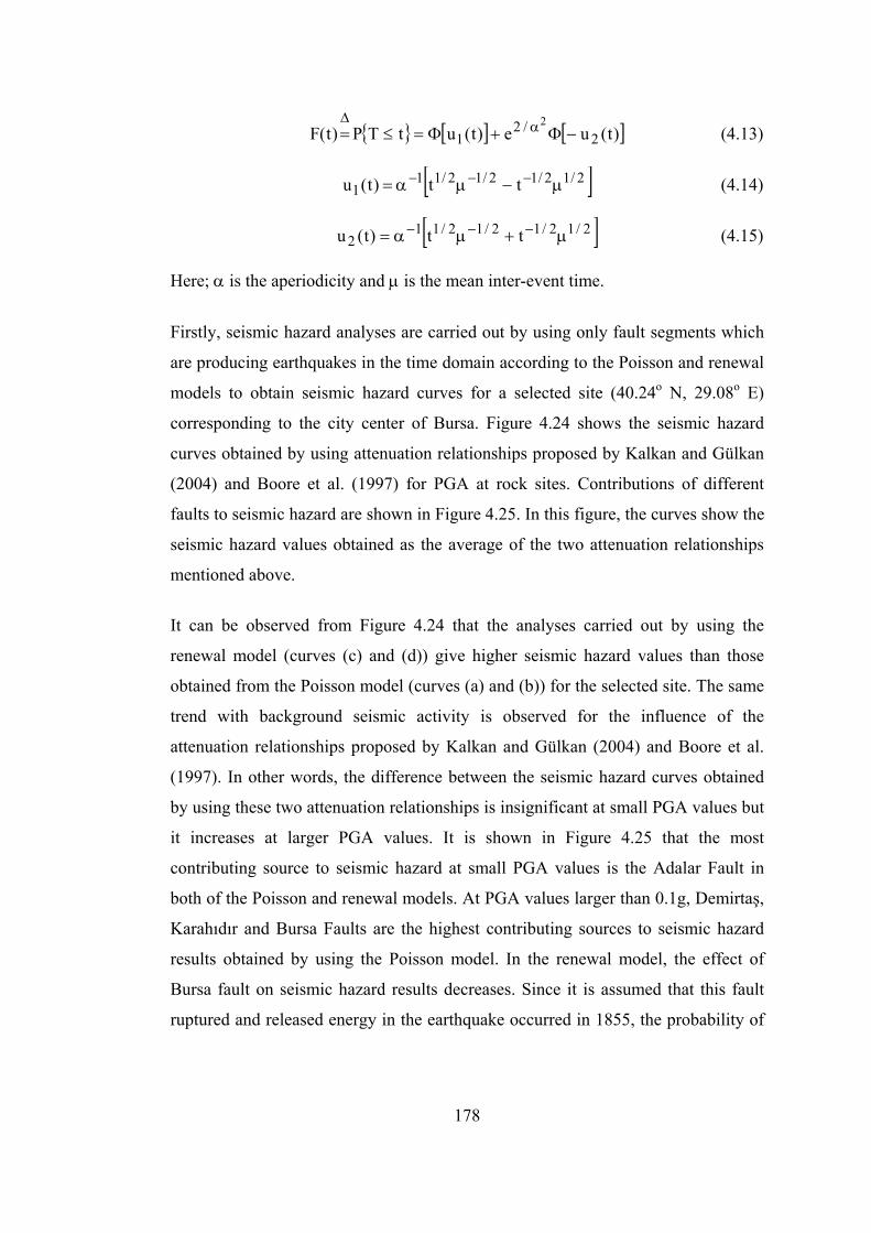
178
{ } [ ] [ ])t(ue)t(utTP)t(F 2/2
12
−Φ+Φ=≤= αΔ
(4.13) [ ]2/12/12/12/11
1 tt)t(u μ−μα= −−− (4.14) [ ]2/12/12/12/11
2 tt)t(u μ+μα= −−− (4.15) Here; α is the aperiodicity and μ is the mean inter-event time.
Firstly, seismic hazard analyses are carried out by using only fault segments which
are producing earthquakes in the time domain according to the Poisson and renewal
models to obtain seismic hazard curves for a selected site (40.24o N, 29.08o E)
corresponding to the city center of Bursa. Figure 4.24 shows the seismic hazard
curves obtained by using attenuation relationships proposed by Kalkan and Gülkan
(2004) and Boore et al. (1997) for PGA at rock sites. Contributions of different
faults to seismic hazard are shown in Figure 4.25. In this figure, the curves show the
seismic hazard values obtained as the average of the two attenuation relationships
mentioned above.
It can be observed from Figure 4.24 that the analyses carried out by using the
renewal model (curves (c) and (d)) give higher seismic hazard values than those
obtained from the Poisson model (curves (a) and (b)) for the selected site. The same
trend with background seismic activity is observed for the influence of the
attenuation relationships proposed by Kalkan and Gülkan (2004) and Boore et al.
(1997). In other words, the difference between the seismic hazard curves obtained
by using these two attenuation relationships is insignificant at small PGA values but
it increases at larger PGA values. It is shown in Figure 4.25 that the most
contributing source to seismic hazard at small PGA values is the Adalar Fault in
both of the Poisson and renewal models. At PGA values larger than 0.1g, Demirtaş,
Karahıdır and Bursa Faults are the highest contributing sources to seismic hazard
results obtained by using the Poisson model. In the renewal model, the effect of
Bursa fault on seismic hazard results decreases. Since it is assumed that this fault
ruptured and released energy in the earthquake occurred in 1855, the probability of

179
future earthquakes sourced from this fault and consequently the annual activity rate
are reduced according to the renewal model.
0.00001
0.0001
0.001
0.01
0.1
1
0.01 0.1 1 10
PGA (g)
Ann
ual F
requ
ency
of E
xcee
danc
e(a)(b)(c)(d)
Figure 4.24 Seismic Hazard Curves Obtained by Using Fault Segments: with Poisson Model and Attenuation Relationships proposed by (a) Boore et al. (1997); (b) Kalkan and Gülkan (2004); and with Renewal Model and Attenuation Relationships proposed by (c) Boore et al. (1997); (d) Kalkan and Gülkan (2004)
In order to investigate the influence of Poisson and renewal models on the variation
of seismic hazard results in space, seismic hazard analyses are carried out by
considering only the contribution of all faults and fault segments in Figure 4.1 at all
grid points with a spacing of 0.02°×0.02° in latitude and longitude in the region
bounded by 26.0˚- 31.8˚ E longitudes and 38.8˚- 42.0˚ N latitudes. Then, seismic
hazard maps are constructed for PGA corresponding to return periods of 475, 1000
and 2475 years. In the analyses, equal weights are given to both attenuation
relationships. Figures 4.26 through 4.28 show seismic hazard maps obtained in this
way based on the Poisson and renewal models.

180
0.000001
0.00001
0.0001
0.001
0.01
0.1
1
0.01 0.1 1 10PGA(g)
Ann
ual F
requ
ency
of E
xcee
danc
e
Adalar Fault
Alaçam Fault
Altıntaş-Kurşunlu Fault
Bursa Fault
Çalı Fault
Demirtaş Fault
Gemlik Fault
Gençali Fault
Gürle Fault
Karahıdır Fault
Koyunhisar Fault
Mudanya Fault
Sayfiye Fault
Soğukpınar Fault
Şükriye Fault
Total Hazard
(a)
0.000001
0.00001
0.0001
0.001
0.01
0.1
1
0.01 0.1 1 10PGA(g)
Ann
ual F
requ
ency
of E
xcee
danc
e
Adalar Fault
Alaçam Fault
Altıntaş-Kurşunlu Fault
Bursa Fault
Demirtaş Fault
Gemlik Fault
Gençali Fault
Gürle Fault
Karahıdır Fault
Kestel Fault Set
Koyunhisar Fault
Mudanya Fault
Sayfiye Fault
Soğukpınar Fault
Şükriye Fault
Total Hazard
(b)
Figure 4.25 Contributions of Different Faults to Seismic Hazard under the Assumption of (a) Poisson Model and (b) Renewal Model

181
26° 27° 28° 29° 30° 31°
26° 27° 28° 29° 30° 31°
39°
40°
41°
42°
39°
40°
41°
42°
(a)
26° 27° 28° 29° 30° 31°
26° 27° 28° 29° 30° 31°
39°
40°
41°
42°
39°
40°
41°
42°
(b)
Figure 4.26 Seismic Hazard Map Obtained for PGA (in g) Corresponding to the Return Period of 475 Years (10% Probability of Exceedance in 50 Years) by Considering Only Faults with (a) Poisson Model, (b) Renewal Model

182
26° 27° 28° 29° 30° 31°
26° 27° 28° 29° 30° 31°
39°
40°
41°
42°
39°
40°
41°
42°
(a)
26° 27° 28° 29° 30° 31°
26° 27° 28° 29° 30° 31°
39°
40°
41°
42°
39°
40°
41°
42°
(b)
Figure 4.27 Seismic Hazard Map Obtained for PGA (in g) Corresponding to the Return Period of 1000 Years (5% Probability of Exceedance in 50 Years) by Considering Only Faults with (a) Poisson Model, (b) Renewal Model
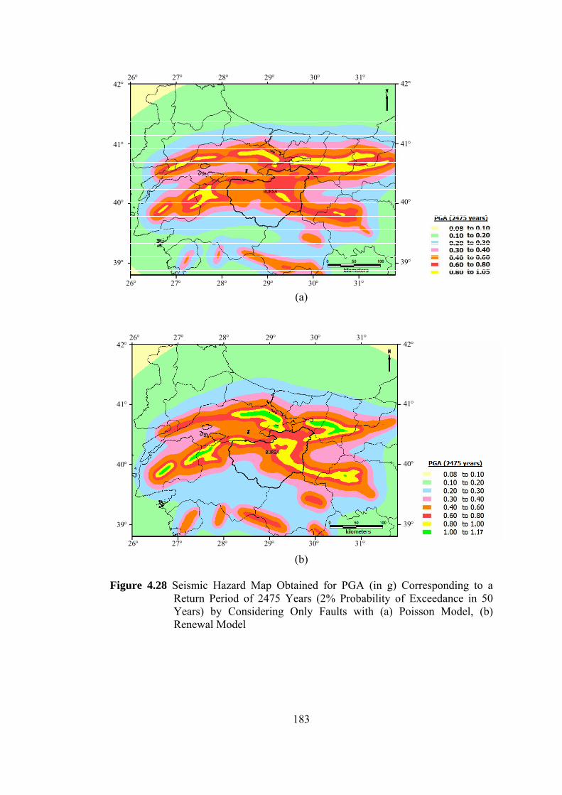
183
26° 27° 28° 29° 30° 31°
26° 27° 28° 29° 30° 31°
39°
40°
41°
42°
39°
40°
41°
42°
(a)
26° 27° 28° 29° 30° 31°
26° 27° 28° 29° 30° 31°
39°
40°
41°
42°
39°
40°
41°
42°
(b)
Figure 4.28 Seismic Hazard Map Obtained for PGA (in g) Corresponding to a
Return Period of 2475 Years (2% Probability of Exceedance in 50 Years) by Considering Only Faults with (a) Poisson Model, (b) Renewal Model

184
In order to visualize the spatial variation of differences between the PGA values
obtained from Poisson and renewal models, the difference is calculated at each grid
point in the region bounded by 26.0˚- 31.8˚ E longitudes and 38.8˚- 42.0˚ N
latitudes by using the following equation;
( ) 100PGA
PGAPGA%Difference
p
pr ×⎟⎟⎠
⎞⎜⎜⎝
⎛ −= (4.16)
where PGAr and PGAp denote the PGA values estimated from renewal and Poisson
models, respectively. The difference with negative sign (-) means that Poisson
model gives higher PGA values than renewal model and that with positive sign
represents the opposite case.
Figures 4.29 through 4.31 show the spatial variation of differences in PGA values
obtained from renewal and Poisson models. It can be observed from these maps that
the renewal model gives more than 25% higher PGA values than the Poisson model,
especially at the regions where the faults have not produced characteristic
earthquakes for a long period of time or date of the last characteristic earthquake is
unknown (e.g. regions around F1, F7, F8, F9, F10, F48, namely Etili, Edincik,
Akhisar, Kütahya, Kaymaz, Simav faults). On the other hand, the PGA values
predicted by the renewal model are more than 25% lower than those of the Poisson
model at the regions where the faults have ruptured and produced large magnitude,
characteristic earthquakes short time before compared with their mean inter-event
times (e.g. regions in the near vicinity of F13, F14, F55, F56, F57, F84, F87, F88,
namely Karadere, Düzce, M.Kemalpaşa, Derecik, Yeniköy, Karamürsel, Gölcük,
Körfez faults). It can be observed from Figures 4.29 and 4.30 that for Bursa
province, the absolute values of the maximum positive and negative differences
between the results obtained from the renewal and Poisson models are less than
55% and 65%, respectively.

185
26° 27° 28° 29° 30° 31°
26° 27° 28° 29° 30° 31°
39°
40°
41°
42°
39°
40°
41°
42°
Figure 4.29 Map Showing the Spatial Variation of the Difference between the PGA
Values Obtained from Renewal and Poisson Models for a Return Period of 475 Years
26° 27° 28° 29° 30° 31°
26° 27° 28° 29° 30° 31°
39°
40°
41°
42°
39°
40°
41°
42°
Figure 4.30 Map Showing the Spatial Variation of the Difference between the PGA
Values Obtained from Renewal and Poisson Models for a Return Period of 2475 Years

186
Figu
re 4
.31
Map
Sho
win
g th
e Sp
atia
l Var
iatio
n of
the
Diff
eren
ce b
etw
een
the
PGA
Val
ues O
btai
ned
from
Ren
ewal
and
Po
isso
n M
odel
s for
a R
etur
n Pe
riod
of 2
475
Yea
rs a
nd F
aults
(Thi
ck B
lack
, Dar
k B
lue,
Dar
k G
reen
Lin
es)
26
° 27
° 28
° 29
° 30
° 31
°
26°
27°
28°
29°
30°
31°
39°
40°
41°
42°
39°
40°
41°
42°

187
4.3.3 “Best Estimate” of Seismic Hazard for the Bursa Province In the previous sections, different assumptions were made in the analyses carried
out to calculate the contributions of background seismic activity and fault segments
to seismic hazard. The results of these analyses are now aggregated through the use
of the logic tree formulation by assigning subjective probabilities to the different
assumptions and/or alternatives as displayed in Table 4.4. “Best estimate” seismic
hazard curve as well as the contribution of different sources (i.e. background
seismic activity and faults) to the seismic hazard for the site (40.24o N, 29.08o E) at
the center of the city of Bursa are shown in Figure 4.32. It can be seen from this
figure that contribution of background seismic activity to seismic hazard is
significant at lower PGA values (i.e. less than 0.03g) that are generally of no
interest from structural engineering point of view. For PGA values larger than 0.1g,
faults contribute most of the seismic hazard at this site.
Table 4.4 Subjective Probabilities Assigned to Different Assumptions
Source Alternatives Subjective
Probabilities Uniform Seismicity 0.5 Spatially Smoothed Seismicity 0.5 The Whole Seismic Database 0.4 Only Main Shocks 0.6 Incomplete Seismic Database 0.3
Background Seismic Activity
Artificially Completed Seismic Database 0.7
Poisson Model 0.3 Faults Renewal Model 0.7 Kalkan and Gülkan (2004) 0.5 Attenuation Relationship Boore et al. (1997) 0.5
Similarly, the results of seismic hazard analyses carried out at each grid point are
aggregated to construct the “best estimate” seismic hazard maps for PGA and SA at
0.2 sec and 1.0 sec periods. Figures 4.33 through 4.41 show “best estimate” seismic

188
hazard maps for the Bursa province for PGA and SA (T=0.2 sec and 1.0 sec)
corresponding to the return periods of 475, 1000 and 2475 years (10%, 2% and 5%
probability of exceedances in 50 years, respectively).
0.00001
0.0001
0.001
0.01
0.1
1
10
0.01 0.1 1 10PGA(g)
Ann
ual F
requ
ency
of E
xcee
danc
eBackground Seismic Activity
Faults
TOTAL
Figure 4.32 Seismic Hazard Curves Resulting from Background Seismic Activity and Faults and the “Best estimate” Seismic Hazard Curve for the Site (40.24o N, 29.08o E) at the City Center of Bursa
Figure 4.33 Best Estimate Seismic Hazard Map of Bursa Province for PGA (in g) Corresponding to the Return Period of 475 Years (10% Probability of Exceedance in 50 Years)

189
Figure 4.34 Best Estimate Seismic Hazard Map of Bursa Province for PGA (in g)
Corresponding to the Return Period of 1000 Years (5% Probability of Exceedance in 50 Years)
Figure 4.35 Best Estimate Seismic Hazard Map of Bursa Province for PGA (in g) Corresponding to the Return Period of 2475 Years (2% Probability of Exceedance in 50 Years)
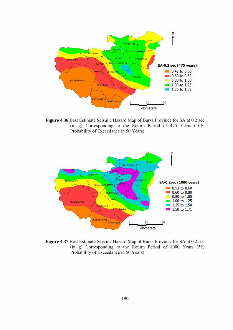
190
Figure 4.36 Best Estimate Seismic Hazard Map of Bursa Province for SA at 0.2 sec
(in g) Corresponding to the Return Period of 475 Years (10% Probability of Exceedance in 50 Years)
Figure 4.37 Best Estimate Seismic Hazard Map of Bursa Province for SA at 0.2 sec
(in g) Corresponding to the Return Period of 1000 Years (5% Probability of Exceedance in 50 Years)

191
Figure 4.38 Best Estimate Seismic Hazard Map of Bursa Province for SA at 0.2 sec
(in g) Corresponding to the Return Period of 2475 Years (2% Probability of Exceedance in 50 Years)
Figure 4.39 Best Estimate Seismic Hazard Map of Bursa Province for SA at 1.0 sec
(in g) Corresponding to the Return Period of 475 Years (10% Probability of Exceedance in 50 Years)
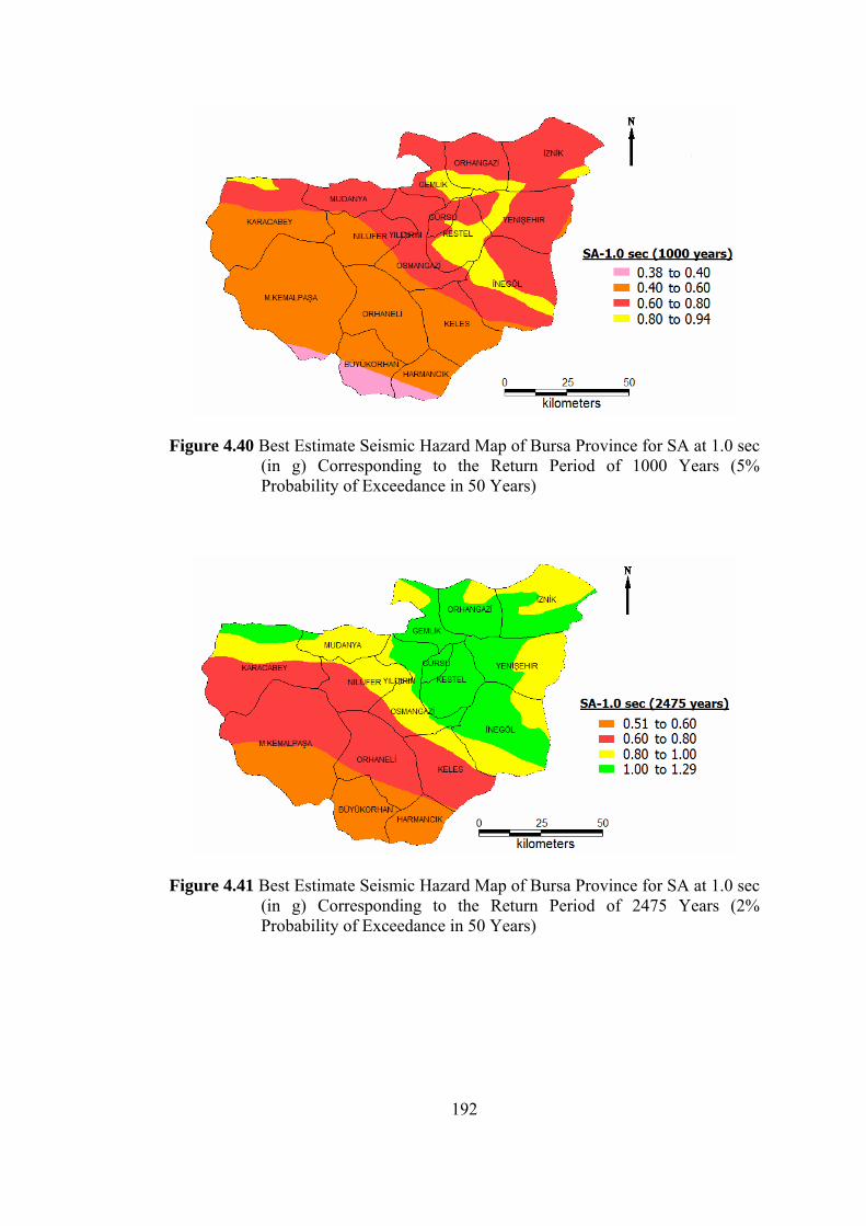
192
Figure 4.40 Best Estimate Seismic Hazard Map of Bursa Province for SA at 1.0 sec
(in g) Corresponding to the Return Period of 1000 Years (5% Probability of Exceedance in 50 Years)
Figure 4.41 Best Estimate Seismic Hazard Map of Bursa Province for SA at 1.0 sec
(in g) Corresponding to the Return Period of 2475 Years (2% Probability of Exceedance in 50 Years)

193
Figure 4.42 shows the seismic hazard map in terms of PGA values corresponding to
a 475 years return period constructed by Yücemen et al. (2006) for Bursa city center
and its near vicinity. For the purpose of comparison of this map with the
corresponding best estimate seismic hazard map constructed in this study, the Bursa
province is cropped out and redrawn as given in Figure 4.43 (a). Since the minimum
and maximum PGA value estimated by Yücemen et al. (2006) for the Bursa
province are 0.2 and 0.62, the legend that shows the range of PGA values is
modified. Figure 4.43 (b) shows the best estimate seismic hazard map obtained in
this study for the Bursa province. It should be noted that the legend displayed in
Figure 4.43 (b) is different from the one given in Figure 4.33, because it is modified
to enable a direct comparison of results obtained in this study with those obtained
by Yücemen et al. (2006). Comparison of the seismic hazard map shown in Figure
4.43 (a) with that given in Figure 4.43 (b) shows that the PGA values predicted in
this study are very close to those obtained in the study of Yücemen et al. (2006).
Smaller PGA values at the regions between Kestel and İnegöl towns are predicted
in this study than those given by Yücemen et al. (2006). This difference could be
due to the fact that in this study Bursa fault is assumed to be ruptured during the
1855 earthquake. Therefore, the probability of occurrence of future characteristic
earthquakes produced by this fault is decreased according to the renewal model.
Additionally, Yücemen et al. (2006) predicted higher PGA values at the region in
M.Kemalpaşa Town. This may be explained by the assumption made in this study
that M.Kemalpaşa and Derecik faults ruptured during the 1964 earthquake. Figure
4.43 (c) shows the current regulatory earthquake zoning map for Bursa. In this map,
the PGA values are predicted to be larger than 0.4g are displayed as 1st degree and
those between 0.3g and 0.4g are as 2nd degree earthquake zone. Compared to the
seismic hazard map obtained in this study, a different pattern is observed for the
distribution of PGA values in this map. This difference may be due to differences in
the seismic source models, earthquake occurrence models and the attenuation
relationships used in these studies. Current regulatory earthquake zoning map was
prepared based on the study conducted by Gülkan et al. (1993). They used area
sources to model the seismic activities related to the main fault zones. The northern

194
part of Bursa is located in the area source used for the description of the seismic
activity in and near vicinity of Marmara and North Aegean. Therefore, this source
has the most significant influence on the spatial distribution of PGA values in the
Bursa province.
Figure 4.42 Seismic Hazard Map Obtained by Yücemen et al. (2006) for PGA Corresponding to the Return Period of 475 Years (10% Probability of Exceedance in 50 Years)

195
(a)
(b)
(c)
Figure 4.43 Seismic Hazard Maps for Bursa Province for PGA Corresponding to
the Return Period of 475 Years (10% Probability of Exceedance in 50 Years) Constructed from the Results of (a) the Study Conducted by Yücemen et al. (2006) (Values are given in terms of g), (b) This Study (Values are given in terms of g); (c) Current Regulatory Earthquake Zoning Map for Bursa (Özmen et al., 1997)

196
CHAPTER 5
SUMMARY AND CONCLUSIONS 5.1 SUMMARY In this study, the sensitivity of seismic hazard results to the different models used
with respect to seismic source description, magnitude distribution, earthquake
occurrence in time and the type of attenuation relationship is investigated, taking
also into consideration the uncertainties associated with these models.
First, the differences in deterministic and probabilistic seismic hazard analyses
approaches are presented with an illustrative example where a site under the threat
of a single fault is considered. Then, effects of uncertainties involved in the
attenuation relationship and alternative assumptions on source modeling, magnitude
distribution and earthquake occurrences in time to the probabilistic seismic hazard
analysis results are investigated for a number of sites. The results were discussed
and a number of recommendations are presented for those who will carry out
probabilistic seismic hazard analysis.
Two case studies were carried out for a large (a country) and a smaller region (a
province) based on real data in order to examine the influence of different
assumptions and/or models to the probabilistic seismic hazard results. These two
case studies also serve for the purpose of illustration of the actual implementation of
the different models and assumptions for seismic source description (line or area),
background seismic activity (background area source with uniform seismicity or
spatially smoothed seismicity model), magnitude distribution (exponential,
characteristic earthquake model proposed by Youngs and Coppersmith (1985) or
maximum magnitude model) and earthquake occurrence in time (Poisson or

197
renewal). In this respect, the application of the logic tree method which is utilized to
combine the results of alternative assumptions and compensate for the epistemic
uncertainties is also demonstrated.
5.2 DISCUSSION OF RESULTS AND MAIN CONCLUSIONS In this section, the results obtained from the case studies carried out in this study are
briefly discussed and the main conclusions drawn based on these results are
presented.
• The seismic hazard results obtained from both deterministic and
probabilistic seismic hazard analyses methodologies are observed to be
sensitive to the choice of the attenuation relationship (ground motion
prediction equation) as well as the variability of ground motion around the
mean prediction curve. This observation is consistent with other similar
studies (e.g. Sabetta et al., 2005). In view of this observation, special
attention should be paid to the choice of the attenuation relationships to be
included in the logic tree method.
• The uncertainty in the ground motion parameter at a specified magnitude
and distance levels is represented by a lognormal distribution. For very long
return periods, the tail of this distribution governs the seismic hazard
estimates. In order to eliminate estimation of physically impossible higher
ground motion values in such extreme cases, the distribution should be
truncated at some upper bounds. Truncation of attenuation residuals and the
bound at which truncation is made affects the seismic hazard results at low
annual probabilities of exceedance. This observation is consistent with other
similar studies (e.g. Bommer et al., 2004).
• Fault-rupture, segmentation and cascade models are used for the spatial
distribution of earthquakes along the line (fault) seismic sources. In the
fault-rupture model, empirical equations are used to estimate the rupture

198
length for a specified magnitude. There is a certain degree of uncertainty in
the rupture length estimated from these relationships. Inclusion of this
uncertainty results in higher seismic hazard values for higher ground motion
parameter levels at the sites located near the central portions of the fault
considered in this study. The effect of rupture length uncertainty on seismic
hazard results decreases as the closest distance to the fault increases. In
addition, increase in standard deviation of the logarithm of rupture length
results in higher exceedance probabilities at higher ground motion parameter
levels at the site which is found to be most sensitive to the uncertainty in
rupture length. Cascade model gives higher exceedance probabilities than
segmentation model at higher ground motion parameter levels whereas
segmentation model results in higher values at lower ground motion
parameter levels.
• For the case that only large magnitude events are taken into consideration,
modeling a fault as a narrow area source (say of 5 km width) results in lower
seismic hazard values than fault (line) source representation of the faults at
the sites near the center of the fault, as expected.
• Line (fault) source model with exponential magnitude distribution may give
higher seismic hazard values than the area source model. Higher differences
are concentrated at the regions along and near vicinity of line sources. On
the other hand, modeling faults having low annual activity rates as area
sources may cause an increase in seismic hazard values at the regions near
the boundaries of area sources compared to line source representation of
faults.
• Based on the same seismicity parameters (i.e., ν and β), use of characteristic
earthquake model proposed by Youngs and Coppersmith (1985) yields
higher seismic hazard results than the classical truncated exponential
distribution for the line (fault) source model. Additionally, lumping the rates

199
uniformly distributed over characteristic magnitudes in the characteristic
earthquake model totally to the maximum magnitude together with
exponentially distributed magnitudes for smaller magnitude earthquakes,
gives higher seismic hazard results, as expected.
• In the renewal model, the date of the last characteristic earthquake occurred
on the faults are used to compute the probability or equivalent mean rate of
occurrence of characteristic earthquakes. For the case that no information is
available on this date, different equations are proposed by Wu et al. (1995)
to compute the mean rate of characteristic earthquakes. For the Brownian
Passage Time model, with aperiodicity value of 0.5, the mean rates of
characteristic earthquakes calculated by the equations proposed for which
date of last characteristic earthquake is known and unknown are observed to
approach each other, for the time period which is some multiples of mean
inter-event time. In cases where the date of last characteristic earthquake is
unknown, the analyst could calculate the rates of characteristic earthquake
from these two equations. When there is no significant difference between
these two values, it is not necessary to spend extra effort to make detailed
investigations for evaluating the date of last characteristic earthquake.
• For background seismic activity, the use of spatially smoothed seismicity
model or the alternative background area source with uniform seismicity
affects the results. For the case studies carried out for Jordan and Bursa, it is
observed that spatially smoothed seismicity model gives higher seismic
hazard values at the regions where the epicenters of earthquakes cluster. On
the other hand, nearly a spatially uniform hazard distribution is obtained
from the seismic hazard analyses carried out by using a background area
source with uniform seismicity. Therefore, background area source model
with uniform seismicity is expected to give higher seismic hazard values
compared to the spatially smoothed seismicity model at the sites located far
away from clustering regions of past earthquake epicenters; i.e. where the

200
epicenters of earthquakes are scarce or no earthquakes have occurred in the
past. In both models, seismicity parameters are determined from the
earthquake catalogs. In addition, the information given in the earthquake
catalogs (year, location of epicenter, depth and magnitude) are one of the
main inputs of the code developed for the computation of seismic hazard by
using spatially smoothed seismicity model by Frankel et al. (1996). The
analyses carried out for the background seismic activity by using both
spatially smoothed seismicity model of Frankel (1995) and a background
area source with uniform seismicity with different combinations of
assumptions on earthquakes in the catalog with respect to completeness and
dependence yield different seismic hazard values. Therefore, the validity of
the results obtained for background seismic activity depends on the
reliability of the earthquake catalog compiled, the method used to identify
main shocks and completeness of the catalog with respect to small
magnitude earthquakes.
• The use of the maximum magnitude model for faults combined with
spatially smoothed seismicity model for background seismic activity and
characteristic earthquake model proposed by Youngs and Coppersmith
(1985) may yield different seismic hazard results depending on the spatial
distribution of past earthquakes and the activity rates assigned to the
maximum magnitude. In cases where the period of available earthquake
catalog is not long enough to predict the frequency of maximum magnitude
earthquake and paleoseismicity data is not available, the activity rates of the
maximum magnitude earthquakes can be calculated by using the maximum
magnitudes, rupture areas and slip rates based on seismic moment balancing
concept. Characteristic earthquake model proposed by Youngs and
Coppersmith (1985) may give higher seismic hazard results in regions where
the activity rates of maximum magnitude earthquakes of faults are lower
than the rates assigned to characteristic events in the characteristic
earthquake model and also a gap exists between the upper bound magnitude

201
of background seismic activity and the maximum magnitude earthquake of
faults.
• Considering the stochastic characteristics of the memoryless Poisson model
and the time-dependent renewal model, it is expected that seismic hazard
results will differ if temporal data for the past seismic activity is taken into
consideration. The main factors that create this difference are the time
passed from the last characteristic earthquake and the inter-event time
distribution of the characteristic earthquakes. For the case study carried out
for Bursa province, it is observed that the renewal model gives higher
seismic hazard values than the Poisson model at the regions where the faults
have not produced characteristic earthquakes for a long period of time with
respect to their mean-inter-event times. On the other hand, the seismic
hazard values predicted by the Poisson model are greater than those of the
renewal model at the regions where the faults have ruptured and produced
large magnitude, characteristic earthquakes short time before, compared
with their mean inter-event times.
• The results obtained by using different assumptions and models can be
combined by employing the logic tree method in order to incorporate the
effects of epistemic uncertainities into the probabilistic seismic hazard
estimates. Since the final result depends on the subjective probabilities
assigned to different alternatives as well as the alternatives taking place in
the logic tree, extreme care should be paid to the process of assigning these
probabilities and selection of the appropriate alternatives. In this respect
expert opinion plays an important role.
• The current trend in probabilistic seismic hazard analysis is to give priority
to the assessment of hazard stemming from the faults. This requires the
appropriate modelling of faults as well as using the proper parameters. The
case studies carried out in this study show that the modeling of faults by area
sources may underestimate seismic hazard especially in the near vicinity of

202
faults. Besides, appropriate magnitude distribution and earthquake
occurrence models consistent with characteristics of faults should be used,
since the results are dependent on these assumptions. These observations
justify the importance of basing the seismic hazard studies on faults with
properly assessed parameters. The assessment of the fault parameters
requires time and money especially for large regions like a country.
Accordingly, in cases of time and money limitations hazard studies can be
carried out on a region and/or province scale, giving priority to high risk
areas.
5.3 RECOMMENDATIONS FOR FUTURE STUDIES In order to improve the results obtained in this dissertation, following
recommendations should be taken into consideration in future studies and research:
• In seismic hazard analysis, regional attenuation relationships (ground
motion estimation equations) derived based on the regional tectonic settings
of the region considered should be used. The derivation of a regional
attenuation relationship depends on the availability of ground motion data
recorded from the past earthquakes occurred in the region. Therefore,
attempts should be made to increase the number of stations and derive local
attenuation relationships based on the data recorded at the stations located in
the region considered.
• Earthquake waves propagate with different characteristics in the directions
parallel and perpendicular to fault rupture. Therefore, the direction of fault
rupture can affect the ground motion. The effect of rupture directivity can be
incorporated into seismic hazard analysis through modifications of the
attenuation relationships. In this study, this effect is not considered in
seismic hazard estimations. The sensitivity of seismic hazard results to this
effect can be investigated in future studies.
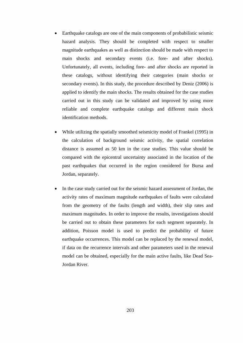
203
• Earthquake catalogs are one of the main components of probabilistic seismic
hazard analysis. They should be completed with respect to smaller
magnitude earthquakes as well as distinction should be made with respect to
main shocks and secondary events (i.e. fore- and after shocks).
Unfortunately, all events, including fore- and after shocks are reported in
these catalogs, without identifying their categories (main shocks or
secondary events). In this study, the procedure described by Deniz (2006) is
applied to identify the main shocks. The results obtained for the case studies
carried out in this study can be validated and improved by using more
reliable and complete earthquake catalogs and different main shock
identification methods.
• While utilizing the spatially smoothed seismicity model of Frankel (1995) in
the calculation of background seismic activity, the spatial correlation
distance is assumed as 50 km in the case studies. This value should be
compared with the epicentral uncertainty associated in the location of the
past earthquakes that occurred in the region considered for Bursa and
Jordan, separately.
• In the case study carried out for the seismic hazard assessment of Jordan, the
activity rates of maximum magnitude earthquakes of faults were calculated
from the geometry of the faults (length and width), their slip rates and
maximum magnitudes. In order to improve the results, investigations should
be carried out to obtain these parameters for each segment separately. In
addition, Poisson model is used to predict the probability of future
earthquake occurrences. This model can be replaced by the renewal model,
if data on the recurrence intervals and other parameters used in the renewal
model can be obtained, especially for the main active faults, like Dead Sea-
Jordan River.

204
• In the case study carried out for the seismic hazard assessment of Bursa
province, the maximum magnitude of faults are generally estimated from
their lengths based on empirical relationships. Therefore, different
segmentation models results in different maximum magnitude values. The
results obtained from alternative segmentation models can be combined by
using the logic tree method.
• In the two case studies, the weights given to alternative models and/or
assumptions in the calculation of “best estimate” seismic hazard values are
all subjective. Different weights could be based on the opinion of experts
who have familiarity with the seismicity and tectonic structure of the region
considered.
• In this study, sensitivity of seismic hazard results to the statistical procedure
used to assess the values of the seismicity parameters of the seismic sources
is not investigated. Regression analysis is applied in the determination of the
slope of the Gutenberg-Richter magnitude recurrence relationship. Other
statistical techniques, such as the maximum likelihood method, can be
applied to assess the values of the seismicity parameters in future studies.
• The cascade model can be applied for the estimation of seismic hazard for
Bursa if detailed information is obtained for identifying the possible multi-
segment rupture of the faults considered in the study.
• In this study, local site conditions are not taken into consideration and all
ground motion parameters are predicted assuming rock site conditions. The
site condition should be considered in future studies.

205
REFERENCES
Abrahamson N. A. and Silva W. J. (1997). Empirical Response Spectral Attenuation Relations for Shallow Crustal Earthquakes, Seismological Research Letters, Vol. 68, No. 1, pp. 94-127.
Aki K. (1966). Generation and Propagation of G-waves from the Niigata Earthquake of June 16,1964, Bull. Earthq. Res. Inst., Vol. 44, pp. 23-88.
Algermissen S. T., Perkins D. M., Isherwood W., Gordon D., Reagor B.G. and Howard C. (1976). Seismic Risk Evaluation of the Balkan Region, Proceedings of the Seminar on Seismic Zoning Maps, Vol. 2, Skopje, Yugoslavia, pp. 172-240.
Al-Tarazi E. (1992). Investigation and Assessment of Seismic Hazard in Jordan and Its Vicinity, Unpublished Ph.D. Thesis, Ruhr University, Bochum, Germany, 194 pp.
Al-Tarazi E. and Sandvol E. (2007). Alternative Models of Seismic Hazard Evaluation along the Jordan–Dead Sea Transform, Earthquake Spectra, Vol. 23, No. 1, pp. 1-19.
Ambraseys N. N. (2001). Reassessment of Earthquakes, 1900-1999, in the Eastern Mediterrean and the Middle East, Geophysical Journal International, Vol. 145, pp. 471-485.
Ambraseys N. N. (2006). Comparison of Frequency of Occurrence of Earthquakes with Slip Rates from Long-Term Seismicity Data: the Cases of Gulf of Corinth, Sea of Marmara and Dead Sea Fault Zone, Geophysical Journal International, Vol. 165, pp. 516-526.
Ambraseys N. N. and Jackson J. A. (1998). Faulting Associated with Historical and Recent Earthquakes in the Eastern Mediterrean Region, Geophysical Journal International, pp. 390-406.
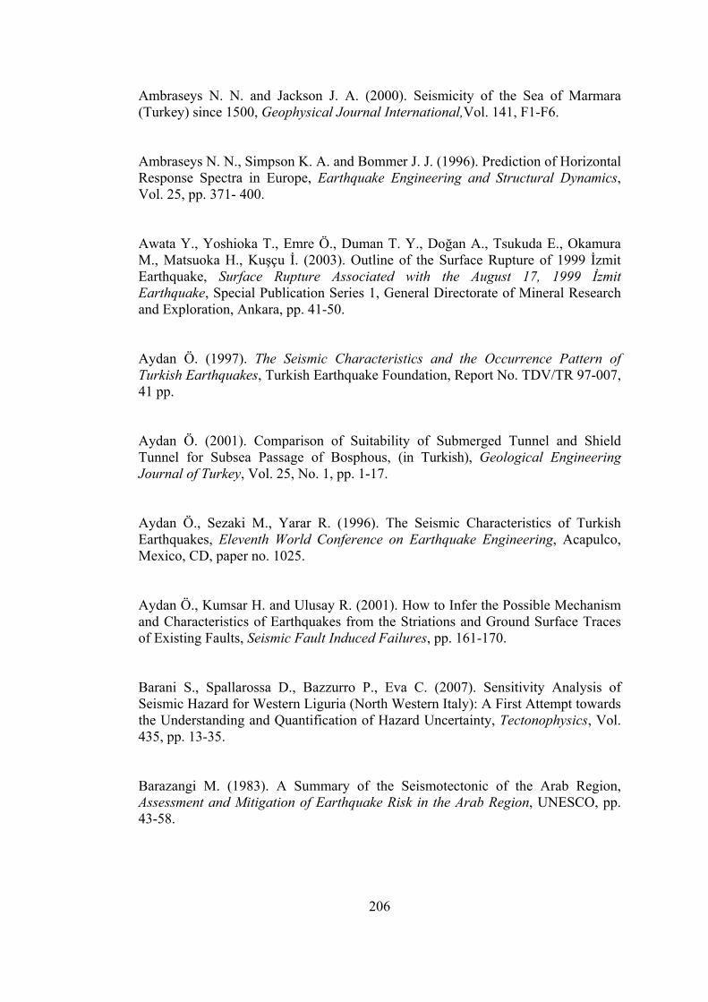
206
Ambraseys N. N. and Jackson J. A. (2000). Seismicity of the Sea of Marmara (Turkey) since 1500, Geophysical Journal International,Vol. 141, F1-F6.
Ambraseys N. N., Simpson K. A. and Bommer J. J. (1996). Prediction of Horizontal Response Spectra in Europe, Earthquake Engineering and Structural Dynamics, Vol. 25, pp. 371- 400.
Awata Y., Yoshioka T., Emre Ö., Duman T. Y., Doğan A., Tsukuda E., Okamura M., Matsuoka H., Kuşçu İ. (2003). Outline of the Surface Rupture of 1999 İzmit Earthquake, Surface Rupture Associated with the August 17, 1999 İzmit Earthquake, Special Publication Series 1, General Directorate of Mineral Research and Exploration, Ankara, pp. 41-50.
Aydan Ö. (1997). The Seismic Characteristics and the Occurrence Pattern of Turkish Earthquakes, Turkish Earthquake Foundation, Report No. TDV/TR 97-007, 41 pp.
Aydan Ö. (2001). Comparison of Suitability of Submerged Tunnel and Shield Tunnel for Subsea Passage of Bosphous, (in Turkish), Geological Engineering Journal of Turkey, Vol. 25, No. 1, pp. 1-17.
Aydan Ö., Sezaki M., Yarar R. (1996). The Seismic Characteristics of Turkish Earthquakes, Eleventh World Conference on Earthquake Engineering, Acapulco, Mexico, CD, paper no. 1025.
Aydan Ö., Kumsar H. and Ulusay R. (2001). How to Infer the Possible Mechanism and Characteristics of Earthquakes from the Striations and Ground Surface Traces of Existing Faults, Seismic Fault Induced Failures, pp. 161-170.
Barani S., Spallarossa D., Bazzurro P., Eva C. (2007). Sensitivity Analysis of Seismic Hazard for Western Liguria (North Western Italy): A First Attempt towards the Understanding and Quantification of Hazard Uncertainty, Tectonophysics, Vol. 435, pp. 13-35.
Barazangi M. (1983). A Summary of the Seismotectonic of the Arab Region, Assessment and Mitigation of Earthquake Risk in the Arab Region, UNESCO, pp. 43-58.

207
Batayneh J. S. F. (1994). Seismic Assessment and Evaluation of Earthquake Hazard in Major Cities in Jordan, Unpublished M.S. Thesis, Jordan University of Science and Technology, Irbid, Jordan, 130 pp.
Ben-Avraham Z. (1985). Structural Framework of the Gulf of Elat (Aqaba), Northern Red Sea, J.Geophys. Res., Vol. 90, pp. 703–726.
Bender F. (1974). Geology of Jordan, Gebrtider Borntraeger, Berlin.
Bender B. (1984). Seismic Hazard Estimation Using A Finite-Fault Rupture Model, Bulletin of the Seismological Society of America, Vol.74, No.5, pp.1899-1923.
Bender B. (1986). Modeling Source Zone Boundary in Seismic Hazard Analysis, Bulletin of the Seismological Society of America., Vol. 76, No. 2, pp. 329-341.
Bender B. and Perkins D. (1982). SEISRISK II. A Computer Program for Seismic Hazard Estimation, U.S. Geological Survey, Open File Report: 82-293.
Bender B. and Perkins D. (1987) SEISRISK III: A Computer Program for Seismic Hazard Estimation, U.S. Geological Survey Bulletin 1772.
Ben-Menahem A. (1979). Earthquake Catalogue for the Middle East (92 B.C-1980 A.D.), Boll. Geofis. Teor. Appl., Vol. 21, No. 81, pp. 245-293.
Ben-Menahem A. (1981). A Seismicity Cycle of 1500 Years on the Dead Sea Rift, Boll. Geofis. Teor. Appl., Vol. 22, No. 92, pp. 349-354.
Bonilla M. G., Mark R. K., Lienkaemper J. J. (1984). Statistical Relations Among Earthquake Magnitude, Surface Rupture Length, and Surface Fault Displacement, Bulletin of the Seismological Society of America, Vol.74, No.6, pp. 2379-2411.
Bommer J. J., Abrahamson N. A., Strasser F. O., Pecker A., Bard P.-Y., Bungum H., Cotton F., Fäh D., Sabetta F., Scherbaum F. and Studer J. (2004). The Challenge of Defining Upper Bounds on Earthquake Ground Motions, Seismological Research Letters, Vol. 75, No. 1, pp. 82-95.
208
Boore D. M., Joyner W. B. and Fumal T. E. (1997). Equations for Estimating Horizontal Response Spectra and Peak Acceleration from Western North American Earthquakes: A Summary of Recent Work, Seismological Research Letters, Vol. 68, No. 1, pp. 128-153.
Brillinger D. R. (1982). Some Bounds for Seismic Risk, Bulletin of the Seismological Society of America, Vol. 72, No. 4, pp. 1403-1410.
Campbell K. W. (1997). Empirical Near-Source Attenuation Relationships for Horizontal and Vertical Components of Peak Ground Acceleration, Peak Ground Velocity, and Pseudo Absolute Acceleration Response Spectra, Seismological Research Letters, Vol. 68, No. 1, pp. 154-179.
Chiang W-L., Guidi G. A., Mortgat C. P., Schoof C. C. and Shah H. C. (1984). Computer Program for Seismic Hazard Analysis. A User Manual (Stanford Seismic Hazard Analysis-STASHA), Report No. 62, The J. A. Blume Earthquake Engineering Center, Stanford University.
Christian J. T., Borjeson R. W. and Tringale P. T. (1978). Probabilistic Evaluation of OBE for Nuclear Plant, Journal of Geotechnical Engineering Division, ASCE, Vol. 104, GT7.
Coburn A.W. and Kuran U. (1985). Emergency Planning and Earthquake Damage Reduction for Bursa Province: A Preliminary Report on Seismic Risk, (in Turkish), The Ministry of Public Works and Settlement, General Directorate of Disaster Affairs, Earthquake Research Department, Ankara, Turkey.
Cornell C. A. (1968). Engineering Seismic Risk Analysis, Bulletin of the Seismological Society of America, Vol. 58, No. 5, pp. 1583-1606.
Cornell C. A. (1971). Probabilistic Analysis of Damage to Structures Under Seismic Load, Dynamic Waves in Civil Engineering, J. Wiley and Sons, N.Y.
Cornell C. A. and Merz H. A. (1974). A Seismic Risk Analysis of Boston, M.I.T., Department of Civil Engineering, Research Report, R 74-2.
209
Cramer C.H., Petersen M. D., Cao T., Toppozada T. R., Reichle M. (2000). A Time-Dependent Probabilistic Seismic-Hazard Model for California, Bulletin of the Seismological Society of America, Vol.90, No.1, pp.1-21.
Deniz A. (2006). Estimation of Earthquake Insurance Premium Rates for Turkey, M.Sc. Thesis, Department of Civil Engineering, METU.
Deniz A. and Yucemen M. S. (2005). Assessment of Seismic Hazard for the Antalya Region Using Stochastic Methods, (in Turkish), Proceedings, Congress on the Civil Engineering Problems of the Antalya Region, pp. 540-551.
Dobbs R. (2008). Personal communication, e-mail correspondence, Risk Engineering Inc., Colorado.
Ellsworth W. L., Matthews M. V., Nadeau R. M., Nishenko S. P., Reasenberg P. A. and Simpson R. W. (1999). A Physically-Based Earthquake Recurrence Model for Estimation of Long-Term Earthquake Probabilities. U.S. Geological Survey, Open-File Report: 99-522.
Emre O. and Awata Y. (2003). Neotectonic Characteristics of the North Anatolian Fault System in the Eastern Marmara, Surface Rupture Associated with the August 17, 1999 İzmit Earthquake, Special Publication Series 1, General Directorate of Mineral Research and Exploration, Ankara, pp.31-39.
ERD-GDDA (2007). Internet page of the Earthquake Research Department, General Directorate of Disaster Affairs, Turkish Republic, The Ministry of Public Works and Settlement, http://sismo.deprem.gov.tr, last accessed date: 20 December 2007.
Erdik M., Demircioğlu M., Sesetyan K., Durukal E. and Siyahi B. (2004). Earthquake Hazard in Marmara Region, Turkey, Soil Dynamics and Earthquake Engineering, Vol. 24, pp. 605-631.
Erentöz, C. and Kurtman, F. (1964). Report on 1964 Manyas Earthquake, Bulletin of the Mineral Research and Exploration Institute of Turkey, No. 63, pp.1-5.

210
Esteva L. (1970). Seismic Risk and Seismic Design Decisions, in Seismic Design for Nuclear Power Plants, Ed. Hansen, R. J., MIT Press, Cambridge, Mass.
Esteva L. and Villaverde R. (1973). Seismic Risk, Design Spectra and Structural Reliability, Proc. 5th World Conference on Earthquake Engineering, Rome, Italy.
Fahmi K. J., Husein Malkawi I. and Al-Zoubi O. Y. (1996). Seismic Engineering Ground Motion Maps for Jordan Employing Local Attenuation Relations, Environmental and Engineering Geosciences, Vol. II, No. 1, pp. 23-33.
Frankel A. (1995). Mapping Seismic Hazard in the Central and Eastern United States, Seismological Research Letters, Vol. 66, No.4, pp. 8-21.
Frankel A., Mueller C., Barnhard T., Perkins D., Leyendecker E., Dickman N., Hanson S. and Hopper M. G. (1996). National Seismic-Hazard Maps: Documentation, U.S. Geological Survey, Open-File Report: 96-532.
Gupta I.D (2002). The State of the Art in Seismic Hazard Analysis, ISET Journal of Earthquake Technology, Vol. 39, No. 4, pp.311-346.
Gülkan P. and Gürpınar A. (1977). Northwestern Anatolian Earthquake Risk , (in Turkish), METU, Earthquake Engineering Research Center, Report No 77-05, Ankara.
Gülkan P. and Kalkan E. (2002). Attenuation Modeling of Recent Earthquakes in Turkey, Journal of Seismology, Vol. 6, pp. 397-409.
Gülkan P., Koçyiğit A., Yücemen M. S., Doyuran V., Başöz N. (1993). A Seismic Zones Map of Turkey Derived From Recent Data, (in Turkish), METU, Earthquake Engineering Research Center, Report No. 93-01.
Gülkan P. and Yücemen M. S. (1975). A Seismic Risk Study of İzmir, Proc. Fifth European Conference on Earthquake Engineering, Vol. 2, İstanbul.
Gülkan P. and Yücemen M. S. (1976). Assessment of Seismic Risk for Akkuyu, Applied Research Report No. 76-04-03-37, METU, Ankara.
211
Hanks T. C. and Kanamori H. (1979). A Moment Magnitude Scale, Journal of Geophysical Research, Vol. 84, pp. 2348-2350.
Hermann R.B. (1977). Recurrence Relations, Earthquake Notes, Vol. 48, pp.47-49.
Husein Malkawi I., Al-Homoud A. and Liang R.Y. (1995). Seismic Hazard Mapping of Jordan, Quarterly J. of Engineering Geology & Hydrogeology, Vol. 28, pp. 75-81.
İnan E., Çolakoğlu Z., Koç N., Bayülke N., Çoruh E. (1996). Earthquake Catalogs with Acceleration Records from 1976 to 1996, (in Turkish), General Directorate of Disaster Affairs, Earthquake Research Department, Ankara, Turkey, 98 pp.
Japan International Cooperation Agency (JICA) and Istanbul Metropolitan Municipality (IMM) (2002). The Study on A Disaster Prevention/Mitigation Basic Plan in Istanbul including Seismic Microzonation in the Republic of Turkey, Final Report, December.
Jiménez M. J. (2004). Jordan Seismic Hazard Mapping, Final Report, Institute of Earth Sciences, “Jaume Almera”.
Joyner W. B. and Boore D. M. (1981). Peak Horizontal Acceleration and Velocity from Strong-Motion Records Including Records from the 1979 Imperial Valley, California Earthquake, Bulletin of the Seismological Society of America, Vol. 71, No. 6, pp. 2011-2038.
Kalkan E. (2007). Personal communication, California Geological Survey, Sacramento.
Kalkan E. and Gülkan P. (2004). Site-Dependent Spectra Derived from Ground Motion Records in Turkey, Earthquake Spectra, Vol. 20, No. 4, pp. 1111-1138.
Kameda H. and Ozaki Y. (1979). A Renewal Process Model for Use in Seismic Risk Analysis, Memoirs of the Faculty of Engineering, Kyoto University, Vol. 41, pp. 11-35.

212
Kiremidjian A. S. and Shah H. C. (1975). Seismic Hazard Mapping of California, The John A. Blume Earthquake Engineering Center, Report No. 21, Department of Civil Engineering, Stanford University.
Koçyiğit A. (2005). Active Fault Investigation in Pilot Municipalities and Their Neighbourhood: Eskişehir, Gemlik, Bandırma, Tekirdağ And Körfez, Final Report, Project: MEER-A3 Microzonation and Hazard Vulnerability Studies For Disaster Mitigation in Pilot Municipalities, 17 pp.
Koçyiğit A. (2006). Personal communication, Department of Geological Engineering, METU, Ankara.
Koçyiğit A. (2007). Personal communication, Department of Geological Engineering, METU, Ankara.
Lomnitz C. (1969). An Earthquake Risk Map of Chili, Proceeding Forth World Conference on Earthquake Engineering, Chili.
Mahmoud S. , Reilinger R., McClusky S., Vernant P., Tealeb A. (2005). GPS Evidence for Northward Motion of the Sinai Block: Implications for E. Mediterranean Tectonics, Earth and Planetary Science Letters, Vol. 238, pp. 217– 224
Matthews M. V., Ellsworth W. L. and Reasenberg P. A. (2002). A Brownian Model for Recurrent Earthquakes, Bulletin of the Seismological Society of America, Vol. 92, No. 6, pp. 2233-2250.
McGuire R. K. (1976). Fortran Computer Program for Seismic Risk Analysis, U.S. Geological Survey, Open-File Report No. 76-67, Denver, Colorado.
McGuire R. K. (1978). FRISK: Computer Program for Seismic Risk Analysis Using Faults as Earthquake Sources, U.S. Geological Survey, Open-File Report 78-1007.
McGuire R. K. (2004). Seismic Hazard and Risk Analysis, EERI, MNO-10, Oakland, CA.
213
Merz H. and Cornell C.A. (1973). Seismic Risk Analysis Based on a Quadratic Magnitude-Frequency Law, Bulletin of the Seismological Society of America, Vol. 63, No. 6, pp. 1999-2006.
Mortgat C. P. and Shah H. C. (1978). A Bayesian Model for Seismic Hazard Mapping-A Case for Algeria, Proceeding of Sixth European Conference on Earthquake Engineering, Vol. 1, Dubrovnik.
Nishenko S. P. and Buland R. (1987). Generic Recurrence Interval Distribution for Earthquake Forecasting, Bulletin of the Seismological Society of America, Vol. 77, pp. 1382-1399.
Ordaz M., Aguilar A. and Arboleda J. (2003). CRISIS2003: Program for Computing Seismic Hazard, Ver. 1.2.100.
Özbey C., Sarı A., Manuel L., Erdik M. and Fahjan Y. (2004). An Empirical Attenuation Relationship for Northwestern Turkey Ground Motion Using A Random Effects Approach, Soil Dynamics and Earthquake Engineering, Vol. 24, pp. 115-125.
Özmen B., Nurlu M. and Güler H. (1997). Examination of Earthquake Zones by Geographic Information System, (in Turkish), The Ministry of Public Works and Settlement, Ankara.
Parsons T. (2004). Recalculated Probability of M ≥7 Earthquakes Beneath the Sea of Marmara, Turkey, Journal of Geophysical Research, Vol. 109.
Reid H. F. (1910). The Mechanics of the Earthquake, The California Earthquake of April 18, 1906, Report of the State Investigation Commission, Vol.2, Carnegie Institution of Washington, Washington, D.C., pp. 16-28.
Reiter L. (1990). Earthquake Hazard Analysis: Issues and Insights, New York, Columbia University Press.
Richter C. F. (1958). Elementary Seismology, W.H. Freeman and Company, San Francisco.

214
Risk Engineering Inc. (2005). EZ-FRISK: 2005, User’s Manual, Version 7.12, Boulder, Colorado.
Risk Engineering Inc. (2006). User’s Manual for FRISK88M Software,Version 2.124, Boulder, Colorado.
Sabetta F., Lucantoni A., Bungum H., Bommer J.J. (2005). Sensitivity of PSHA Results to Ground Motion Prediction Relations and Logic-Tree Weights, Soil Dynamics and Earthquake Engineering, Vol. 25, pp.317–329.
Sadigh K., Chang C.-Y., Egan J. A., Makdisi F. and Youngs R. R. (1997). Attenuation Relationships for Shallow Crustal Earthquakes Based on California Strong Motion Data, Seismological Research Letters, Vol. 68, No. 1, pp. 180-189.
Şaroğlu F., Emre Ö. and Kuşçu İ. (1992). Active fault map of Turkey, General Directorate of Mineral Research and Exploration, Turkey.
Schwartz D. P. and Coppersmith K. J. (1984). Fault Behavior and Characteristic Earthquakes: Examples from The Wasatch and San Andreas Fault Zones, Journal of Geophysical Research, Vol. 89, No. B7, pp. 5681-5698.
Shah H. C., Mortgat C. P. Kiremidjian A. and Zsutty T. C. (1975). A Study of Seismic Risk for Nicaragua, Part I, The John A. Blume Earthquake Engineering Centre, Stanford University.
Shapira, A. (1981). Assessment of the Potential Earthquake Risk in Israel and Adjacent Areas, Israel J. of Earth Sciences, Vol. 30, pp. 135-141.
Shlien S. and Toksöz M. N. (1970). Frequency-Magnitude Statistics of Earthquake Occurrence, Earthquake Notes, No. 41.
SSHAC Report (1997), Recommendations for Probabilistic Seismic Hazard Analysis: Guidance on Uncertainty and Use of Experts, NUREG/CR-6372, Vol. 1, Lawrence Livermore National Laboratory, Livermore, CA.

215
Thenhaus P. C. and Campbell K. W. (2003). Seismic Hazard Analysis, Chapter 8, Earthquake Engineering Hand Book, Wai-Fah Chen and Charles Schawthorn (editors), CRC Press.
Ulusay R., Tuncay E., Sönmez H. and Gökçeoğlu C. (2004). An Attenuation Relationship Based on Turkish Strong Motion Data and Iso-Acceleration Map of Turkey, Engineering Geology, Vol.74, pp. 265-291.
Vanmarcke E. H. and Cornell C. A. (1969). Analysis of Uncertainty in Ground Motion and Structural Response Due to Earthquakes, M.I.T., Department of Civil Engineering, Research Report, R 69-24.
Wells D. L. and Coppersmith K. J. (1994). New Empirical Relationships Among Magnitude, Rupture Length, Rupture Width, Rupture Area and Surface Displacement, Bulletin of the Seismological Society of America, Vol. 84, No. 4, pp. 974-1002.
Working Group on California Earthquake Probabilities (WGCEP) (1995). Seismic Hazards in Southern California: Probable Earthquakes, 1994 to 2024, Bulletin of the Seismological Society of America, Vol. 85, No. 2, pp. 379-439.
Working Group on California Earthquake Probabilities (WGCEP) (1999). Earthquake Probabilities in the San Francisco Bay Region: 2000 to 2030-A Summary of Findings, U.S. Geological Survey, Open-File Report 99-517.
Wu S.-C., Cornell C. A. and Winterstein S. R. (1995). A Hybrid Recurrence Model and Its Implication on Seismic Hazard Results, Bulletin of the Seismological Society of America, Vol. 85, No. 1, pp. 1-16.
Youngs R. R. and Coppersmith K. J. (1985). Implications of Fault Slip Rates and Earthquake Recurrence Models to Probabilistic Seismic Hazard Estimates, Bulletin of the Seismological Society of America, Vol. 75, No. 4, pp. 939-964.
Yücemen M. S. (1982), Seismic Risk Analysis , (in Turkish), Middle East Technical University, Ankara, 160 pp.

216
Yücemen M.S. (1992). Seismic Hazard Maps for Jordan and Vicinity, Natural Hazards, Kluwer Academic Publishers, Vol. 6, No. 3, pp. 201-226.
Yücemen M. S. (1995). Assessment of Seismic Hazard for Jordan Considering the Uncertainty in the Location of Seismic Sources, Proc. International Conference on Earthquake Engineering, Amman, Jordan, Vol. I, pp. 135-144.
Yücemen M. S. and Gülkan P. (1994) Seismic Hazard Analysis with Randomly Located Sources, Natural Hazards, Vol. 9, Kluwer Academic Publishers, pp. 215-233.
Yücemen M. S., Koçyiğit A., Yakut A., Gencoğlu S. (2006) Guidelines for the Development of Seismic Hazard Maps, Technical Report prepared for General Directorate of Disaster Affairs, Ankara, 78 pp.

217
APPENDIX A
GRAPHS SHOWING THE DIFFERENCE BETWEEN THE SEISMIC HAZARD RESULTS OBTAINED BY IGNORING AND
CONSIDERING RUPTURE LENGTH UNCERTAINTY In this appendix, the graphs which show the difference between the seismic hazard
results obtained by ignoring rupture length uncertainty and considering it as a
function of the number of rupture lengths are presented. In these graphs, the PGA
values are normalized by median PGA value obtained from DSHA for magnitude
6.3 in order to reduce the effect of attenuation of PGA values with distance on
results.
-2
0
2
4
6
8
10
12
0 0.5 1 1.5 2 2.5 3
PGA/Median PGA
Diff
eren
ce (%
)
nr=2nr=4nr=8nr=16nr=100
Figure A.1 The Variation of the Difference Between the Seismic Hazard Results Obtained by Ignoring Rupture Length Uncertainty and Considering it As a Function of Number of Rupture Lengths per Magnitude (Site1a)
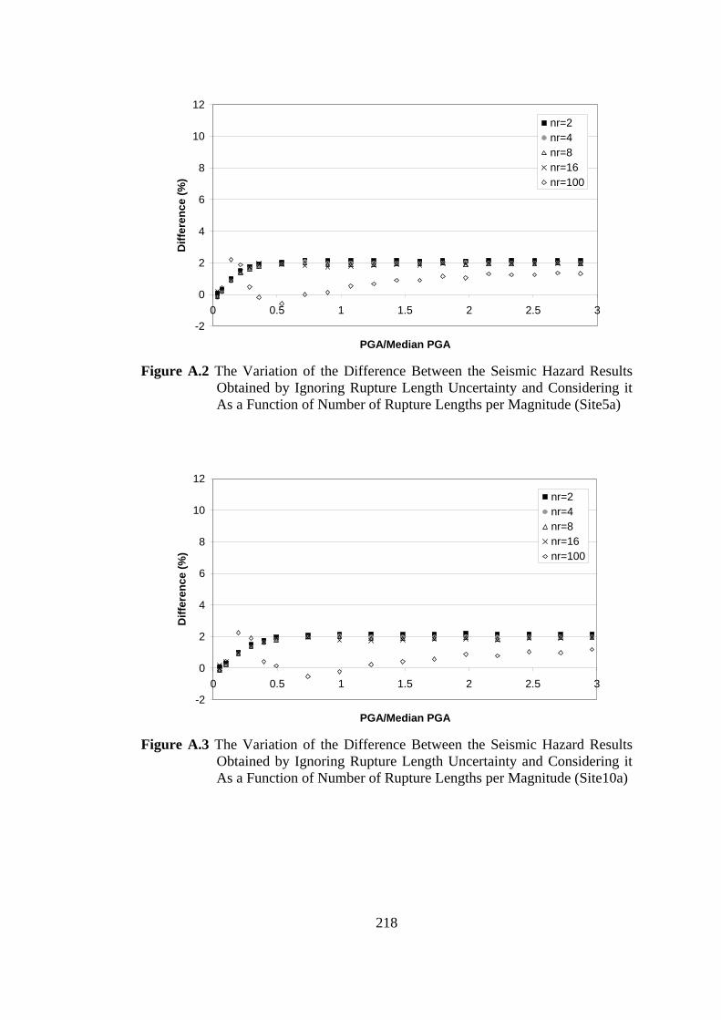
218
-2
0
2
4
6
8
10
12
0 0.5 1 1.5 2 2.5 3
PGA/Median PGA
Diff
eren
ce (%
)
nr=2nr=4nr=8nr=16nr=100
Figure A.2 The Variation of the Difference Between the Seismic Hazard Results
Obtained by Ignoring Rupture Length Uncertainty and Considering it As a Function of Number of Rupture Lengths per Magnitude (Site5a)
-2
0
2
4
6
8
10
12
0 0.5 1 1.5 2 2.5 3
PGA/Median PGA
Diff
eren
ce (%
)
nr=2nr=4nr=8nr=16nr=100
Figure A.3 The Variation of the Difference Between the Seismic Hazard Results
Obtained by Ignoring Rupture Length Uncertainty and Considering it As a Function of Number of Rupture Lengths per Magnitude (Site10a)

219
-2
0
2
4
6
8
10
12
0 0.5 1 1.5 2 2.5 3
PGA/Median PGA
Diff
eren
ce (%
)
nr=2nr=4nr=8nr=16nr=100
Figure A.4 The Variation of the Difference Between the Seismic Hazard Results
Obtained by Ignoring Rupture Length Uncertainty and Considering it As a Function of Number of Rupture Lengths per Magnitude (Site1b)
-2
0
2
4
6
8
10
12
0 0.5 1 1.5 2 2.5 3
PGA/Median PGA
Diff
eren
ce (%
)
nr=2nr=4nr=8nr=16nr=100
Figure A.5 The Variation of the Difference Between the Seismic Hazard Results
Obtained by Ignoring Rupture Length Uncertainty and Considering it As a Function of Number of Rupture Lengths per Magnitude (Site5b)
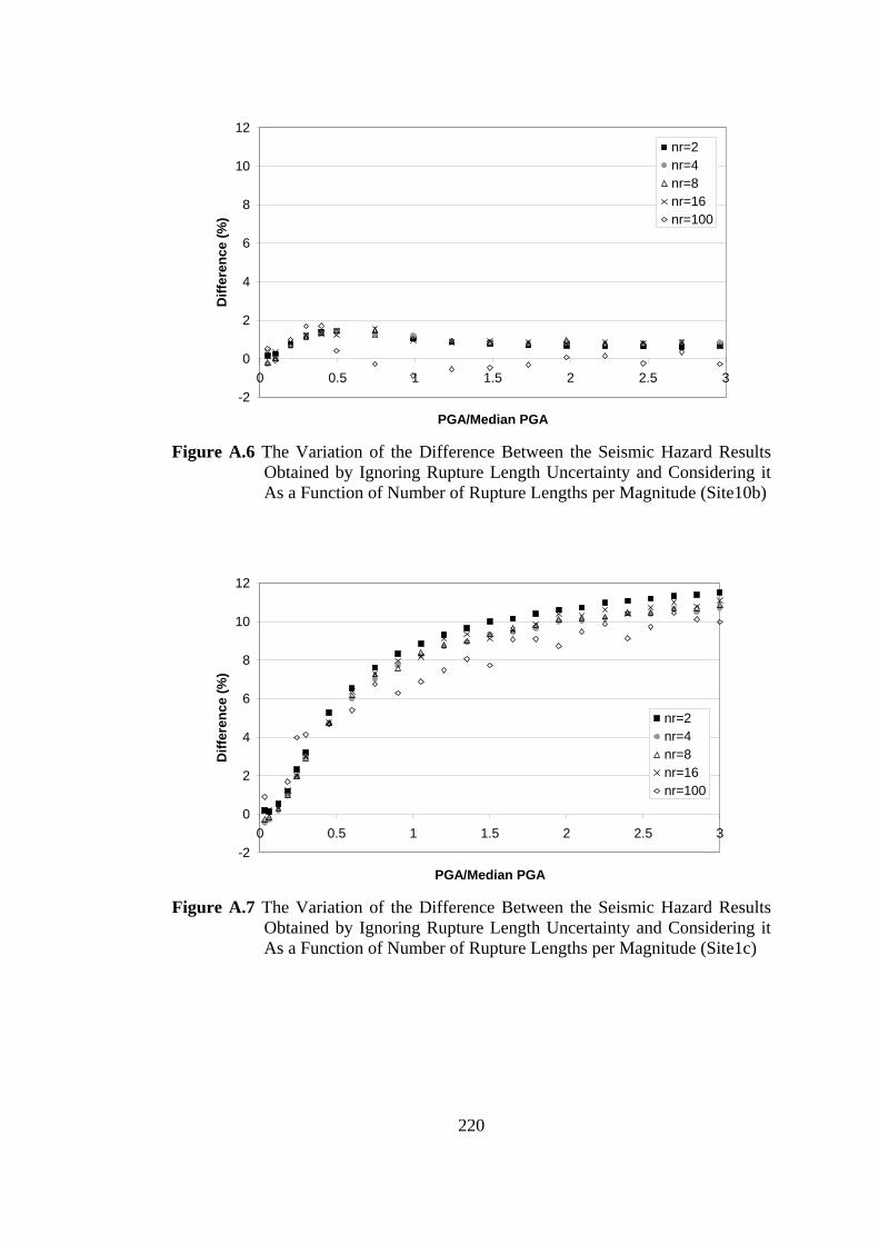
220
-2
0
2
4
6
8
10
12
0 0.5 1 1.5 2 2.5 3
PGA/Median PGA
Diff
eren
ce (%
)
nr=2nr=4nr=8nr=16nr=100
Figure A.6 The Variation of the Difference Between the Seismic Hazard Results
Obtained by Ignoring Rupture Length Uncertainty and Considering it As a Function of Number of Rupture Lengths per Magnitude (Site10b)
-2
0
2
4
6
8
10
12
0 0.5 1 1.5 2 2.5 3
PGA/Median PGA
Diff
eren
ce (%
)
nr=2nr=4nr=8nr=16nr=100
Figure A.7 The Variation of the Difference Between the Seismic Hazard Results
Obtained by Ignoring Rupture Length Uncertainty and Considering it As a Function of Number of Rupture Lengths per Magnitude (Site1c)

221
-2
0
2
4
6
8
10
12
0 0.5 1 1.5 2 2.5 3
PGA/Median PGA
Diff
eren
ce (%
)
nr=2nr=4nr=8nr=16nr=100
Figure A.8 The Variation of the Difference Between the Seismic Hazard Results
Obtained by Ignoring Rupture Length Uncertainty and Considering it As a Function of Number of Rupture Lengths per Magnitude (Site 5c)
-2
0
2
4
6
8
10
12
0 0.5 1 1.5 2 2.5 3
PGA/Median PGA
Diff
eren
ce (%
)
nr=2nr=4nr=8nr=16nr=100
Figure A.9 The Variation of the Difference Between the Seismic Hazard Results
Obtained by Ignoring Rupture Length Uncertainty and Considering it As a Function of Number of Rupture Lengths per Magnitude (Site10c)

222
-2
0
2
4
6
8
10
12
0 0.5 1 1.5 2 2.5 3
PGA/Median PGA
Diff
eren
ce (%
)
nr=2nr=4nr=8nr=16nr=100
Figure A.10 The Variation of the Difference Between the Seismic Hazard Results
Obtained by Ignoring Rupture Length Uncertainty and Considering it As a Function of Number of Rupture Lengths per Magnitude (Site1d)
-2
0
2
4
6
8
10
12
0 0.5 1 1.5 2 2.5 3
PGA/Median PGA
Diff
eren
ce (%
)
nr=2nr=4nr=8nr=16nr=100
Figure A.11 The Variation of the Difference Between the Seismic Hazard Results
Obtained by Ignoring Rupture Length Uncertainty and Considering it As a Function of Number of Rupture Lengths per Magnitude (Site5d)

223
-2
0
2
4
6
8
10
12
0 0.5 1 1.5 2 2.5 3
PGA/Median PGA
Diff
eren
ce (%
)
nr=2nr=4nr=8nr=16nr=100
Figure A.12 The Variation of the Difference Between the Seismic Hazard Results
Obtained by Ignoring Rupture Length Uncertainty and Considering it As a Function of Number of Rupture Lengths per Magnitude (Site10d)
-2
0
2
4
6
8
10
12
0 0.5 1 1.5 2 2.5 3
PGA/Median PGA
Diff
eren
ce (%
)
nr=2nr=4nr=8nr=16nr=100
Figure A.13 The Variation of the Difference Between the Seismic Hazard Results
Obtained by Ignoring Rupture Length Uncertainty and Considering it As a Function of Number of Rupture Lengths per Magnitude (Site1e)

224
-2
0
2
4
6
8
10
12
0 0.5 1 1.5 2 2.5 3
PGA/Median PGA
Diff
eren
ce (%
)
nr=2nr=4nr=8nr=16nr=100
Figure A.14 The Variation of the Difference Between the Seismic Hazard Results
Obtained by Ignoring Rupture Length Uncertainty and Considering it As a Function of Number of Rupture Lengths per Magnitude (Site5e)
-2
0
2
4
6
8
10
12
0 0.5 1 1.5 2 2.5 3
PGA/Median PGA
Diff
eren
ce (%
)
nr=2nr=4nr=8nr=16nr=100
Figure A.15 The Variation of the Difference Between the Seismic Hazard Results
Obtained by Ignoring Rupture Length Uncertainty and Considering it As a Function of Number of Rupture Lengths per Magnitude (Site10e)

225
APPENDIX B
EARTHQUAKE CATALOG PREPARED FOR JORDAN
There are 175 earthquakes treated as main shocks (independent events) with
magnitudes (ML) greater than or equal to 4.0 in this catalog.
Table B.1 Main Shocks in the Earthquake Catalog Prepared for Jordan
No Year Month Day Latitude (Degree)
Longitude(Degree)
Depth Ms Mb ML
1 1900 1 5 35.2000 33.2000 6.3 6.2 2 1903 3 29 32.2000 35.4000 5.25 5.5 3 1907 6 10 33.7000 35.4000 3.4 4.2 4 1907 7 22 33.7000 35.4000 3.4 4.2 5 1910 10 7 33.9000 36.2000 10 3.4 4.2 6 1918 9 29 35.2000 34.7000 6.7 6.5 7 1919 8 19 35.2000 34.7000 5.25 5.5 8 1921 4 20 34.0000 33.0000 5.6 5.75 9 1923 2 27 32.7000 35.4000 3.55 4.3
10 1924 2 18 34.5000 34.0000 6 6 11 1924 2 27 32.7000 36.2000 20 4.7 5.1 12 1924 9 13 30.8000 35.5000 4.4 4.9 13 1927 7 11 32.1000 35.5000 6 6 14 1927 7 11 32.0000 35.5000 6.5 6.3 15 1927 9 24 30.4000 35.1000 15 4.55 5 16 1927 12 12 34.5000 34.7000 5.25 5.5 17 1930 5 9 34.1000 32.2000 5.6 5.75 18 1930 5 21 32.0000 35.5000 3.5 4.3 19 1930 9 14 34.6000 36.6000 3.7 4.5 20 1937 10 12 31.5000 35.5000 3.4 4.2 21 1940 1 27 32.8000 35.1000 3.7 4.4 22 1940 7 24 34.5000 34.5000 5.7 5.8 23 1940 9 2 31.3000 35.6000 3.7 4.5 24 1941 1 20 35.5000 33.6000 100 6.5 6.6

226
Table B.1 (Continued) Main Shocks in the Earthquake Catalog Prepared for Jordan
No Year Month Day Latitude
(Degree) Longitude(Degree)
Depth Ms Mb ML
25 1942 9 28 34.4000 36.6000 3.4 4.2 26 1943 9 10 32.6000 35.4000 4.1 4.7 27 1944 10 7 32.7000 35.5000 10 3.55 4.3 28 1949 10 28 33.0000 33.5000 3.7 4.4 29 1951 1 30 32.4000 33.4000 5.55 5.7 30 1951 8 5 34.2000 36.0000 4.1 4.7 31 1952 3 22 27.2000 34.5000 4.55 5 32 1952 12 28 32.8000 35.4000 3.4 4.2 33 1953 2 1 33.5000 32.0000 4.55 5 34 1953 9 10 34.9000 32.2000 6.7 6.5 35 1953 11 3 32.0000 35.6000 3.25 4.1 36 1954 9 13 31.0000 35.4000 33 4.55 5 37 1956 3 16 33.6150 35.5100 5.25 5.5 38 1956 3 16 33.6150 35.5100 6 6 39 1956 12 18 31.6300 35.5200 5.15 5.4 40 1957 7 29 34.8000 36.9000 3.4 4.2 41 1957 11 3 32.5000 35.5000 3.8 4.5 42 1958 2 14 31.3000 35.6000 3.4 4.2 43 1959 6 13 34.9000 32.3900 5.3 5.5 44 1960 1 28 33.0000 35.5000 3.55 4.3 45 1961 9 15 34.9800 33.8300 33 6 6 46 1964 6 28 34.7700 32.3500 63 4.7 4.15 4.7 47 1964 9 23 34.2000 32.7000 67 4.3 4.8 48 1965 1 25 34.5600 32.8400 20 4.8 4.3 4.8 49 1965 3 17 34.6400 32.3000 52 4.6 4 4.6 50 1965 5 2 33.4000 35.5000 3.55 4.3 51 1965 6 8 34.0300 33.7000 33 3.4 4.2 52 1966 3 6 34.5000 32.7000 3.85 4.5 53 1967 4 17 34.5000 32.8400 4.6 4 4.6 54 1967 6 15 34.0900 32.4300 52 4.7 4.15 4.7 55 1968 3 26 34.0800 35.4700 37 4.8 4.3 4.8 56 1968 12 4 31.8000 35.6000 3.4 4.2 57 1969 3 31 27.6100 33.9100 33 6.1 6.1 6.1 58 1970 3 18 34.4200 32.4900 38 3.85 4.5 59 1970 9 29 33.2000 34.4000 4.1 3.3 4.1 60 1970 10 5 35.0400 39.0000 34 4.8 4.3 4.8 61 1970 10 8 31.7000 35.3000 10 4 4.6 62 1970 12 26 34.2000 33.7000 4.0 3.1 4 63 1971 4 16 33.6400 35.4300 10 4.5 3.85 4.5
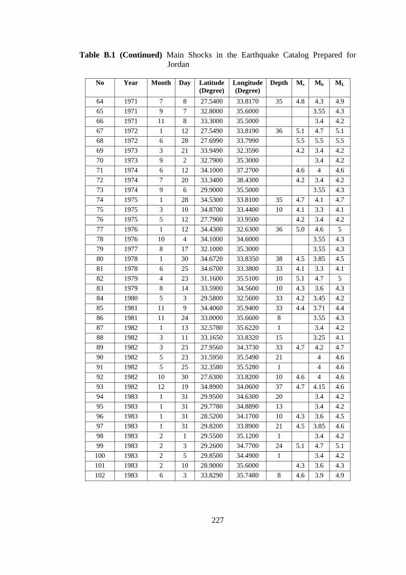
227
Table B.1 (Continued) Main Shocks in the Earthquake Catalog Prepared for Jordan
No Year Month Day Latitude
(Degree) Longitude(Degree)
Depth Ms Mb ML
64 1971 7 8 27.5400 33.8170 35 4.8 4.3 4.9 65 1971 9 7 32.8000 35.6000 3.55 4.3 66 1971 11 8 33.3000 35.5000 3.4 4.2 67 1972 1 12 27.5490 33.8190 36 5.1 4.7 5.1 68 1972 6 28 27.6990 33.7990 5.5 5.5 5.5 69 1973 3 21 33.9490 32.3590 4.2 3.4 4.2 70 1973 9 2 32.7900 35.3000 3.4 4.2 71 1974 6 12 34.1000 37.2700 4.6 4 4.6 72 1974 7 20 33.3400 38.4300 4.2 3.4 4.2 73 1974 9 6 29.9000 35.5000 3.55 4.3 74 1975 1 28 34.5300 33.8100 35 4.7 4.1 4.7 75 1975 3 10 34.8700 33.4400 10 4.1 3.3 4.1 76 1975 5 12 27.7900 33.9500 4.2 3.4 4.2 77 1976 1 12 34.4300 32.6300 36 5.0 4.6 5 78 1976 10 4 34.1000 34.6000 3.55 4.3 79 1977 8 17 32.1000 35.3000 3.55 4.3 80 1978 1 30 34.6720 33.8350 38 4.5 3.85 4.5 81 1978 6 25 34.6700 33.3800 33 4.1 3.3 4.1 82 1979 4 23 31.1600 35.5100 10 5.1 4.7 5 83 1979 8 14 33.5900 34.5600 10 4.3 3.6 4.3 84 1980 5 3 29.5800 32.5600 33 4.2 3.45 4.2 85 1981 11 9 34.4060 35.9400 33 4.4 3.71 4.4 86 1981 11 24 33.0000 35.6600 8 3.55 4.3 87 1982 1 13 32.5780 35.6220 1 3.4 4.2 88 1982 3 11 33.1650 33.8320 15 3.25 4.1 89 1982 3 23 27.9560 34.3730 33 4.7 4.2 4.7 90 1982 5 23 31.5950 35.5490 21 4 4.6 91 1982 5 25 32.3580 35.5280 1 4 4.6 92 1982 10 30 27.6300 33.8200 10 4.6 4 4.6 93 1982 12 19 34.8900 34.0600 37 4.7 4.15 4.6 94 1983 1 31 29.9500 34.6300 20 3.4 4.2 95 1983 1 31 29.7780 34.8890 13 3.4 4.2 96 1983 1 31 28.5200 34.1700 10 4.3 3.6 4.5 97 1983 1 31 29.8200 33.8900 21 4.5 3.85 4.6 98 1983 2 1 29.5500 35.1200 1 3.4 4.2 99 1983 2 3 29.2600 34.7700 24 5.1 4.7 5.1 100 1983 2 5 29.8500 34.4900 1 3.4 4.2 101 1983 2 10 28.9000 35.6000 4.3 3.6 4.3 102 1983 6 3 33.8290 35.7480 8 4.6 3.9 4.9

228
Table B.1 (Continued) Main Shocks in the Earthquake Catalog Prepared for Jordan
No Year Month Day Latitude
(Degree) Longitude(Degree)
Depth Ms Mb ML
103 1983 6 12 28.5540 33.1300 29 5.0 4.8 5.2 104 1983 6 15 27.2200 34.4700 5 3.3 4.1 105 1983 7 19 29.0740 34.6510 2 3.3 4.1 106 1983 9 24 34.6240 33.3150 46 4.5 3.9 4.5 107 1983 9 28 34.8600 32.7200 58 4.2 3.4 4.2 108 1983 10 31 34.9000 33.6500 75 4.4 3.7 4.4 109 1984 3 2 28.7100 35.2340 1 3.3 4.1 110 1984 3 28 34.7500 33.5800 34 5.0 4.3 5 111 1984 3 29 30.2100 32.1900 8 4.8 4.3 4.8 112 1984 4 6 30.3800 33.9180 9 4 4.6 113 1984 4 7 33.7600 32.5110 27 4.5 3.85 4.4 114 1984 4 18 28.7200 33.2200 27 3.3 4.1 115 1984 5 23 32.2500 34.9900 1 3.3 4.1 116 1984 8 24 32.6910 35.1920 13 5.1 4.2 5.1 117 1984 9 7 27.1000 34.9600 2 3.45 4.2 118 1984 10 18 33.1600 35.6100 4 4.3 119 1984 11 5 32.1100 35.3650 4 4.4 3.45 4.2 120 1985 1 13 27.0500 34.6700 26 3.45 4.2 121 1985 1 25 31.8900 35.5900 18 4.6 4.4 4.9 122 1985 2 28 27.7200 33.7150 10 4.5 3.8 4.5 123 1985 4 26 34.0200 36.6900 18 4.3 124 1985 6 6 34.8500 32.6500 42 4.5 3.85 4.4 125 1985 11 16 35.0300 33.4000 41 3.55 4.3 126 1985 12 31 30.4100 35.0500 10 4.3 127 1985 12 31 29.1300 34.9000 9 4.8 4.3 5.1 128 1986 7 7 34.8050 33.6690 49 4.6 4 4.6 129 1986 7 30 34.6710 32.3070 37 4.9 4.1 5 130 1986 8 7 29.1540 34.7200 3.7 4.4 131 1987 1 2 30.4800 32.2210 24 5.0 4.55 5 132 1987 1 10 34.6590 33.2820 37 4.3 3.6 4.3 133 1987 2 18 34.9490 32.2940 49 4.6 4 4.6 134 1987 4 27 31.2500 35.5200 11 4.3 3.6 4.2 135 1987 10 18 29.5100 35.1870 10 4.4 3.7 4.7 136 1987 10 23 31.0000 35.5100 10 4.2 3.4 4.1 137 1987 11 9 34.7350 32.8770 26 4.5 3.85 4.5 138 1988 1 30 32.1900 35.4700 14 4.1 139 1988 6 5 27.9800 33.7300 10 4.6 4 4.8 140 1989 3 31 31.8700 37.5350 28 5.0 4.6 5.2 141 1989 10 4 28.0800 33.7300 10 3.7 4.4
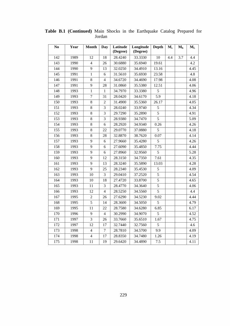
229
Table B.1 (Continued) Main Shocks in the Earthquake Catalog Prepared for Jordan
No Year Month Day Latitude
(Degree) Longitude(Degree)
Depth Ms Mb ML
142 1989 12 18 28.4240 33.3330 10 4.4 3.7 4.4 143 1990 4 26 30.6880 35.6940 19.61 4.2 144 1990 9 13 32.0250 34.4910 13.16 4.45 145 1991 1 6 31.5610 35.6930 23.58 4.8 146 1991 8 4 34.6720 34.4690 17.98 4.08 147 1991 9 28 31.0860 35.5380 12.51 4.06 148 1993 1 1 34.7970 33.3380 5 4.96 149 1993 7 31 28.0420 34.6170 5.9 4.18 150 1993 8 2 31.4900 35.5360 26.17 4.05 151 1993 8 3 28.0240 33.9740 5 4.34 152 1993 8 3 29.7290 35.2890 5 4.91 153 1993 8 3 28.9380 34.7470 5 5.09 154 1993 8 6 28.2920 34.9340 0.26 4.26 155 1993 8 22 29.0770 37.0880 5 4.18 156 1993 8 28 32.8870 38.7620 0.07 4.14 157 1993 9 6 27.9660 35.4280 5 4.26 158 1993 9 6 27.6090 35.4850 7.75 4.44 159 1993 9 6 27.8960 32.9560 5 5.28 160 1993 9 12 28.3150 34.7350 7.61 4.35 161 1993 9 13 28.3240 35.5890 13.03 4.28 162 1993 9 25 28.2340 35.4530 5 4.09 163 1993 10 3 29.0410 37.2520 5 4.54 164 1993 10 18 27.4720 33.8700 5 4.65 165 1993 11 3 28.4770 34.3640 5 4.06 166 1993 12 4 28.5250 34.5560 5 4.4 167 1995 2 26 27.6290 34.5230 9.02 4.44 168 1995 5 14 28.3600 34.5050 5 4.79 169 1995 11 22 28.7580 34.6280 6.85 6.17 170 1996 9 4 30.2990 34.9070 5 4.52 171 1997 3 26 33.7660 35.6510 1.67 4.75 172 1997 12 17 32.7440 32.7560 5 4.6 173 1998 4 7 28.7810 34.5700 9.9 4.09 174 1998 4 17 28.8350 34.7480 1.26 4.19 175 1998 11 19 29.6420 34.4890 7.5 4.11

230
APPENDIX C
SEISMIC HAZARD MAPS FOR JORDAN BASED ON DIFFERENT MODELS
For the assumptions related to the different models (i.e. Model 1, 2, 3, 4) please refer to Section 3.3.2.
Figure C.1 Seismic Hazard Map Obtained from Model 1 for PGA at 10%
Probability of Exceedance in 50 Years (475 Years Return Period)
32° 34° 36° 38° 40°
32° 34° 36° 38° 40°
28°
30°
32°
34°
36°
28°
30°
32°
34°
36°

231
Figure C.2 Seismic Hazard Map Obtained from Model 1 for PGA at 5% Probability of Exceedance in 50 Years (1000 Years Return Period)
Figure C.3 Seismic Hazard Map Obtained from Model 1 for PGA at 2%
Probability of Exceedance in 50 Years (2475 Years Return Period)
32° 34° 36° 38° 40°
32° 34° 36° 38° 40°
28°
30°
32°
34°
36°
28°
30°
32°
34°
36°
32° 34° 36° 38° 40°
32° 34° 36° 38° 40°
28°
30°
32°
34°
36°
28°
30°
32°
34°
36°

232
Figure C.4 Seismic Hazard Map Obtained from Model 2 for PGA at 10%
Probability of Exceedance in 50 Years (475 Years Return Period)
Figure C.5 Seismic Hazard Map Obtained from Model 2 for PGA at 5%
Probability of Exceedance in 50 Years (1000 Years Return Period)
32° 34° 36° 38° 40°
32° 34° 36° 38° 40°
28°
30°
32°
34°
36°
28°
30°
32°
34°
36°
32° 34° 36° 38° 40°
32° 34° 36° 38° 40°
28°
30°
32°
34°
36°
28°
30°
32°
34°
36°

233
Figure C.6 Seismic Hazard Map Obtained from Model 2 for PGA at 2%
Probability of Exceedance in 50 Years (2475 Years Return Period)
Figure C.7 Seismic Hazard Map Obtained from Model 3 for PGA at 10% Probability of Exceedance in 50 Years (475 Years Return Period)
32° 34° 36° 38° 40°
32° 34° 36° 38° 40°
28°
30°
32°
34°
36°
28°
30°
32°
34°
36°
32° 34° 36° 38° 40°
32° 34° 36° 38° 40°
28°
30°
32°
34°
36°
28°
30°
32°
34°
36°

234
Figure C.8 Seismic Hazard Map Obtained from Model 3 for PGA at 5%
Probability of Exceedance in 50 Years (1000 Years Return Period)
Figure C.9 Seismic Hazard Map Obtained from Model 3 for PGA at 2%
Probability of Exceedance in 50 Years (2475 Years Return Period)
32° 34° 36° 38° 40°
32° 34° 36° 38° 40°
28°
30°
32°
34°
36°
28°
30°
32°
34°
36°
32° 34° 36° 38° 40°
32° 34° 36° 38° 40°
28°
30°
32°
34°
36°
28°
30°
32°
34°
36°

235
Figure C.10 Seismic Hazard Map Obtained from Model 4 for PGA at 10% Probability of Exceedance in 50 Years (475 Years Return Period)
Figure C.11 Seismic Hazard Map Obtained from Model 4 for PGA at 5% Probability of Exceedance in 50 Years (1000 Years Return Period)
32° 34° 36° 38° 40°
32° 34° 36° 38° 40°
28°
30°
32°
34°
36°
28°
30°
32°
34°
36°
32° 34° 36° 38° 40°
32° 34° 36° 38° 40°
28°
30°
32°
34°
36°
28°
30°
32°
34°
36°

236
Figure C.12 Seismic Hazard Map Obtained from Model 4 for PGA at 2%
Probability of Exceedance in 50 Years (2475 Years Return Period)
32° 34° 36° 38° 40°
32° 34° 36° 38° 40°
28°
30°
32°
34°
36°
28°
30°
32°
34°
36°

237
APPENDIX D
MAIN SEISMIC DATABASE COMPILED FOR BURSA FROM THE CATALOGS OF EARTHQUAKE RESEARCH
DEPARTMENT, GENERAL DIRECTORATE OF DISASTER AFFAIRS
This seismic database contains earthquakes with moment magnitude (Mw) ≥ 4.5
occurred within the rectangular region bounded by 26.0˚- 31.8˚ E longitudes and
38.8˚- 42.0˚ N latitudes.
Table D.1 All Earthquakes in the Seismic Database Compiled for Bursa
No Year Month Day Longitude (Degree)
Latitude (Degree)
Depth (km)
Mw-(ave)
1 1901 5 12 30.5 39.8 15 5.5 2 1903 4 4 28 39 20 5.8 3 1905 1 11 27.9 39.6 15 5.5 4 1905 4 15 29 40.2 6 5.8 5 1905 4 30 30.5 39.8 22 5.7 6 1905 5 1 31.1 39.9 5.5 7 1905 10 22 31 41 27 5.6 8 1907 1 22 29 41 12 5.2 9 1907 8 21 30.1 40.7 15 5.8
10 1908 11 16 26.5 41.5 20 5.2 11 1912 8 9 27.2 40.6 16 6.8 12 1912 8 10 27.1 40.6 15 6.2 13 1912 8 10 27.1 40.6 15 5.7 14 1912 8 11 27.1 40.6 15 5.2 15 1912 8 11 27.2 40.6 5.5 16 1912 9 16 26.8 40.1 5.5 17 1912 10 21 27 40.5 15 5.2 18 1912 10 21 27 40.5 15 5.4 19 1914 3 22 26 40 15 5.2 20 1916 4 26 27 39.2 10 5.1 21 1917 4 10 27.1 40.6 15 5.7 22 1917 8 8 27 39 15 5.2

238
Table D.1 (Continued) All Earthquakes in the Seismic Database Compiled for Bursa
No Year Month Day Longitude
(Degree) Latitude (Degree)
Depth (km)
Mw-(ave)
23 1917 12 27 26 40.5 5.5 24 1919 5 27 31.02 39.13 10 5.7 25 1919 10 13 28 41.5 12 5.2 26 1919 11 18 26.71 39.26 10 6.6 27 1920 1 9 26.2 41.8 20 5.6 28 1920 11 27 26.5 39.3 14 5.5 29 1921 7 24 26.5 38.8 22 5.6 30 1922 6 19 26 40.5 5.5 31 1923 5 29 30 41 25 5.8 32 1923 10 26 28.6 41.2 24 5.5 33 1924 1 22 28.4 39.51 80 5.7 34 1924 4 14 27.8 39 15 5.3 35 1924 12 22 27.7 39.6 15 5.7 36 1925 4 29 27.7 39.6 15 5.3 37 1925 6 10 29 41 8 5.2 38 1925 6 24 30.39 40.88 10 5.3 39 1925 9 14 31 39 5.5 40 1925 9 20 31 39 5.5 41 1926 11 13 26 39 20 5.1 42 1926 12 16 30.72 40.13 10 5.9 43 1926 12 20 31 39 5.5 44 1927 1 4 29.8 39.5 15 5.1 45 1928 1 24 30.86 40.99 10 5.7 46 1928 5 2 29.14 39.64 10 6.1 47 1928 5 3 26.8 40.8 4 5.1 48 1928 5 6 30.5 39.8 12 5.5 49 1929 4 5 31.23 41.61 10 5.4 50 1929 4 5 31.5 41.5 33 5.4 51 1929 4 27 31.43 40.51 70 5.4 52 1929 10 10 27.46 41.11 15 5.2 53 1931 7 12 26.34 39.15 10 5.7 54 1932 10 15 30.6 40.9 15 5.2 55 1933 2 5 31.5 41.5 5.2 56 1933 5 15 31.09 41.26 60 5.3 57 1934 7 14 26 39.5 10 5.1 58 1935 1 4 27.49 40.4 30 6.3 59 1935 1 4 27.65 40.12 12 5.3 60 1935 1 4 27.17 40.37 5 5.2 61 1935 1 4 27.45 40.3 20 6.2 62 1935 10 22 27.21 40.31 10 5.6 63 1938 7 2 27.88 40.17 10 5.5 64 1939 7 25 29.52 39.75 50 5.6 65 1939 7 31 29.6 39.8 10 5.4 66 1939 8 2 29.48 39.75 50 5.7 67 1939 8 3 29.68 39.75 50 5.8

239
Table D.1 (Continued) All Earthquakes in the Seismic Database Compiled for Bursa
No Year Month Day Longitude
(Degree) Latitude (Degree)
Depth (km)
Mw-(ave)
68 1939 8 9 29.81 39.91 60 5.6 69 1939 9 15 29.56 39.76 20 5.9 70 1939 9 22 26.94 39.07 10 6.4 71 1939 10 19 29.5 39.82 10 5.7 72 1940 6 13 30.17 41.34 30 5.3 73 1940 8 19 30.09 40.13 40 5.2 74 1941 2 9 28.27 40.13 15 5.3 75 1942 2 5 29.8 38.9 17 5.7 76 1942 6 16 27.8 40.8 20 5.8 77 1942 8 12 27.64 39.13 50 5.4 78 1942 8 12 27.7 39.1 17 5.4 79 1942 10 28 28.19 39.27 10 5.7 80 1942 10 28 27.8 39.1 50 6 81 1942 10 28 27.79 39.46 10 5.8 82 1942 11 15 28.58 39.55 10 6.1 83 1943 4 14 29.64 39.62 40 5.5 84 1943 6 20 30.51 40.85 10 6.3 85 1943 6 20 30.73 40.84 10 5.8 86 1943 9 6 31.35 40.21 10 5.5 87 1943 9 8 30.4 40.7 5 5 88 1944 2 1 31.27 40.7 10 5.5 89 1944 2 2 31.44 40.74 40 5.6 90 1944 4 5 31.12 40.84 10 5.8 91 1944 6 25 29.55 38.97 57 5.8 92 1944 10 6 26.56 39.48 40 6.5 93 1944 10 6 26.5 39.3 18 5.5 94 1944 10 7 26.58 39.22 10 5.6 95 1945 2 9 31.2 40.5 5.5 96 1948 11 9 26.4 40.1 90 5.3 97 1948 11 13 29.02 40.23 60 5.8 98 1948 12 13 30 41 15 5.1 99 1949 1 4 27.9 38.9 14 5.2
100 1949 2 5 29.35 39.89 40 5.6 101 1949 11 28 30.9 40.6 5.3 102 1950 11 28 28.05 39.73 40 5.6 103 1951 3 12 31.8 42 5.3 104 1951 9 15 28.02 40.15 40 5.5 105 1952 1 22 30.4 40.8 15 5.1 106 1952 1 26 26.9 39.1 30 5.3 107 1952 3 13 28.14 41.02 11 5.5 108 1952 3 19 28.64 39.6 40 5.7 109 1953 3 18 27.36 39.99 10 6.7 110 1953 3 18 27.4 40 30 5.5 111 1953 3 18 27.83 40.02 10 5.3 112 1953 3 18 27.59 39.96 30 5.7
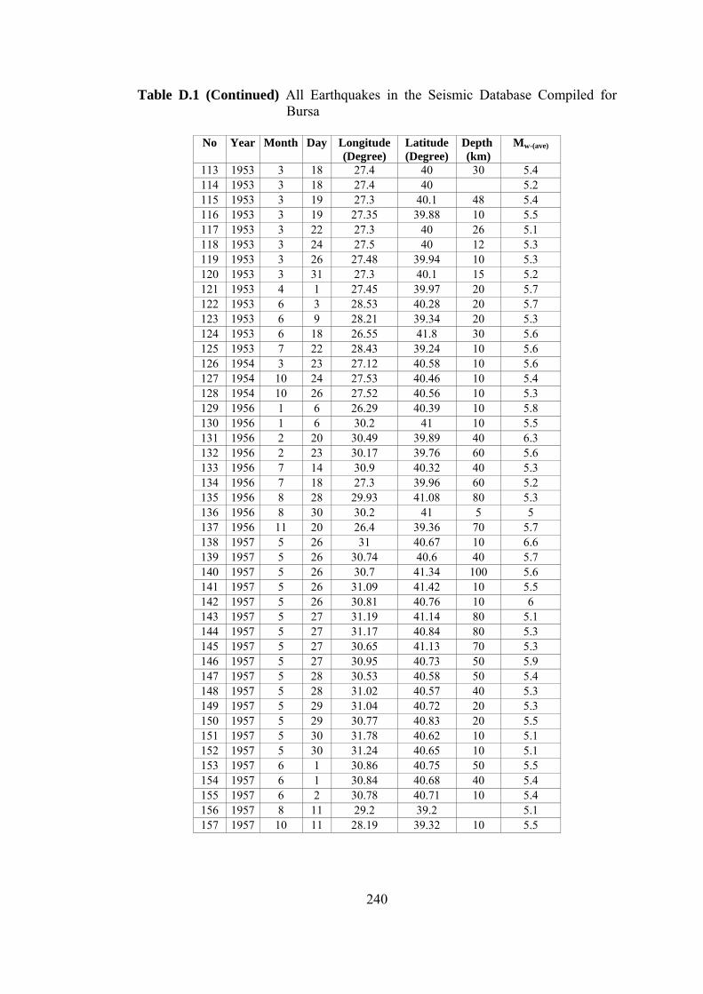
240
Table D.1 (Continued) All Earthquakes in the Seismic Database Compiled for Bursa
No Year Month Day Longitude
(Degree) Latitude (Degree)
Depth (km)
Mw-(ave)
113 1953 3 18 27.4 40 30 5.4 114 1953 3 18 27.4 40 5.2 115 1953 3 19 27.3 40.1 48 5.4 116 1953 3 19 27.35 39.88 10 5.5 117 1953 3 22 27.3 40 26 5.1 118 1953 3 24 27.5 40 12 5.3 119 1953 3 26 27.48 39.94 10 5.3 120 1953 3 31 27.3 40.1 15 5.2 121 1953 4 1 27.45 39.97 20 5.7 122 1953 6 3 28.53 40.28 20 5.7 123 1953 6 9 28.21 39.34 20 5.3 124 1953 6 18 26.55 41.8 30 5.6 125 1953 7 22 28.43 39.24 10 5.6 126 1954 3 23 27.12 40.58 10 5.6 127 1954 10 24 27.53 40.46 10 5.4 128 1954 10 26 27.52 40.56 10 5.3 129 1956 1 6 26.29 40.39 10 5.8 130 1956 1 6 30.2 41 10 5.5 131 1956 2 20 30.49 39.89 40 6.3 132 1956 2 23 30.17 39.76 60 5.6 133 1956 7 14 30.9 40.32 40 5.3 134 1956 7 18 27.3 39.96 60 5.2 135 1956 8 28 29.93 41.08 80 5.3 136 1956 8 30 30.2 41 5 5 137 1956 11 20 26.4 39.36 70 5.7 138 1957 5 26 31 40.67 10 6.6 139 1957 5 26 30.74 40.6 40 5.7 140 1957 5 26 30.7 41.34 100 5.6 141 1957 5 26 31.09 41.42 10 5.5 142 1957 5 26 30.81 40.76 10 6 143 1957 5 27 31.19 41.14 80 5.1 144 1957 5 27 31.17 40.84 80 5.3 145 1957 5 27 30.65 41.13 70 5.3 146 1957 5 27 30.95 40.73 50 5.9 147 1957 5 28 30.53 40.58 50 5.4 148 1957 5 28 31.02 40.57 40 5.3 149 1957 5 29 31.04 40.72 20 5.3 150 1957 5 29 30.77 40.83 20 5.5 151 1957 5 30 31.78 40.62 10 5.1 152 1957 5 30 31.24 40.65 10 5.1 153 1957 6 1 30.86 40.75 50 5.5 154 1957 6 1 30.84 40.68 40 5.4 155 1957 6 2 30.78 40.71 10 5.4 156 1957 8 11 29.2 39.2 5.1 157 1957 10 11 28.19 39.32 10 5.5

241
Table D.1 (Continued) All Earthquakes in the Seismic Database Compiled for Bursa
No Year Month Day Longitude
(Degree) Latitude (Degree)
Depth (km)
Mw-(ave)
158 1957 10 24 29.75 40.06 10 5.3 159 1957 12 26 29.72 40.83 10 5.6 160 1958 11 23 30.69 40.49 10 5.2 161 1959 4 2 29.41 40.5 20 5.3 162 1959 7 26 27.54 40.91 10 5.7 163 1959 8 6 29.2 40.4 5 164 1959 11 19 26.65 38.89 10 5.7 165 1960 3 6 26.5 41.3 22 5 166 1960 3 9 26.5 40.5 5 167 1961 3 28 30.19 39.82 10 5.5 168 1961 8 24 27.99 39.41 10 5.1 169 1961 11 28 26.1 39.99 80 5.6 170 1962 4 19 28.84 40.75 10 5.1 171 1962 9 14 28.17 39.57 40 5.2 172 1963 3 29 26.15 40.29 50 5.6 173 1963 4 28 27.82 39.32 30 5.3 174 1963 9 18 29.12 40.77 40 6.2 175 1963 9 24 28.9 40.84 10 5.4 176 1964 10 6 28.16 40.24 23 6 177 1964 10 6 28.23 40.3 34 7.4 178 1965 8 23 26.17 40.51 33 5.6 179 1966 8 21 27.4 40.33 12 4.7 180 1967 4 7 31 40 4.5 181 1967 7 22 30.69 40.67 7.4 182 1967 7 22 30.8 40.7 6 5.6 183 1967 7 22 30.53 40.73 4.7 184 1967 7 22 30.62 40.66 26 4.9 185 1967 7 22 30.51 40.72 35 5.3 186 1967 7 22 30.53 40.64 30 4.7 187 1967 7 22 30 41 4.8 188 1967 7 30 30.52 40.72 18 6 189 1968 2 19 26.4 39.8 5.6 190 1968 11 3 29.11 38.81 23 4.7 191 1969 3 3 27.5 40.08 6.5 192 1969 3 23 28.48 39.14 9 6.5 193 1969 3 24 28.51 39.11 30 5.1 194 1969 3 25 28.41 39.06 28 4.9 195 1969 3 25 28.44 39.25 37 6.2 196 1969 3 25 28 39 5.1 197 1969 3 25 28.49 39.17 34 4.7 198 1969 3 28 28.45 39.13 37 4.9 199 1969 4 30 28.52 39.12 8 5.1 200 1969 10 7 28.4 39.2 13 4.9 201 1969 10 7 28.54 39.16 49 4.9 202 1969 10 13 28.38 39.17 9 4.9

242
Table D.1 (Continued) All Earthquakes in the Seismic Database Compiled for Bursa
No Year Month Day Longitude
(Degree) Latitude (Degree)
Depth (km)
Mw-(ave)
203 1970 3 28 29.51 39.21 18 7.4 204 1970 3 28 29.46 39.28 17 4.7 205 1970 3 28 29.56 39.15 31 4.7 206 1970 3 28 29.76 39.07 32 5.1 207 1970 3 28 29.7 38.9 5.4 208 1970 3 28 30.3 39.5 5.6 209 1970 3 28 30.7 39.3 4.7 210 1970 3 28 30.7 39.5 4.5 211 1970 3 28 31.5 38.9 4.5 212 1970 3 28 31.1 39.5 4.5 213 1970 3 29 29.74 39.06 29 5.3 214 1970 3 30 29.26 39.34 16 5.3 215 1970 3 31 29.16 39.12 43 5.1 216 1970 3 31 30.1 39 15 4.5 217 1970 4 1 28.8 38.9 54 4.9 218 1970 4 1 29.27 39.32 35 4.7 219 1970 4 2 29.6 38.9 41 5.3 220 1970 4 4 30.3 38.9 4.6 221 1970 4 6 28.54 39.19 33 5.3 222 1970 4 7 29.61 39.07 33 6 223 1970 4 7 29.32 39.34 33 5.3 224 1970 4 16 29.91 39.02 31 6 225 1970 4 16 29.95 38.98 43 4.7 226 1970 4 19 29.76 39.03 18 6.2 227 1970 4 19 29.8 39.03 24 6 228 1970 4 19 30.9 40 5.2 229 1970 4 19 30.7 39.6 5.1 230 1970 4 19 30.7 39.6 5.6 231 1970 4 19 31 39.5 4.6 232 1970 4 20 31.5 39.9 256 5.8 233 1970 4 22 29.77 39.02 37 5.1 234 1970 4 23 30.01 38.94 32 4.9 235 1970 4 23 28.65 39.13 28 5.6 236 1970 4 24 29.85 39.01 32 4.7 237 1970 4 24 29.7 39.01 44 5.3 238 1970 4 27 29.58 38.96 33 4.7 239 1970 5 11 29.39 39.08 5.8 240 1970 5 14 29.1 39.02 38 5.3 241 1970 9 9 29.52 38.97 4.7 242 1970 12 20 29.24 39.36 26 5.1 243 1971 2 15 29.36 39.19 32 4.9 244 1971 2 23 27.32 39.62 5.1 245 1971 4 13 29.8 39.03 41 5.3 246 1971 5 25 29.71 39.05 16 6.7 247 1971 6 10 29.63 39.02 33 5.1

243
Table D.1 (Continued) All Earthquakes in the Seismic Database Compiled for Bursa
No Year Month Day Longitude
(Degree) Latitude (Degree)
Depth (km)
Mw-(ave)
248 1971 11 6 29.78 39.02 16 5.1 249 1972 3 14 29.47 39.32 38 5.8 250 1972 4 26 26.36 39.43 18 5.1 251 1972 4 26 26.33 39.45 25 4.7 252 1972 5 28 30.04 38.96 29 4.7 253 1975 3 17 26.24 40.4 5 4.7 254 1975 3 17 26.08 40.48 5.1 255 1975 3 27 26.12 40.45 6.2 256 1976 5 8 29.1 39.33 33 4.7 257 1976 8 22 29.03 39.35 23 4.7 258 1978 6 15 27.68 40.79 28 4.6 259 1979 7 18 28.65 39.66 7 5.5 260 1980 8 2 27.42 38.93 5.8 261 1981 3 12 28.09 40.8 4.8 262 1981 12 26 28.74 40.15 4.9 263 1982 7 12 27.83 41 25 4.5 264 1982 12 26 28.26 39.32 5 4.9 265 1982 12 27 28.27 39.34 11 4.7 266 1983 2 1 28.94 40.2 3 4.7 267 1983 7 5 27.21 40.33 7 6.1 268 1983 10 21 29.35 40.14 12 5.3 269 1983 11 2 29.36 40.1 4 4.5 270 1983 11 6 29.32 39.33 14 4.6 271 1984 7 29 26 40.4 10 5 272 1985 3 29 26.57 38.8 26 4.7 273 1985 12 1 27.7 39.29 10 4.6 274 1985 12 18 26.17 39.2 17 5.3 275 1987 8 6 26.26 39.25 19 4.5 276 1988 4 24 28.24 40.88 11 5.3 277 1989 8 15 26.25 39.22 10 5.1 278 1991 2 12 28.82 40.8 10 5 279 1992 3 22 28.35 40.2 25 5 280 1993 3 31 28.04 39.14 2 4.5 281 1993 11 1 29.95 38.94 7 4.9 282 1993 12 12 28.79 41.55 28 4.9 283 1994 2 8 27.8 40.8 11 4.5 284 1995 4 13 27.65 40.85 27 4.5 285 1998 3 5 27.3 39.55 23 4.6 286 1999 7 24 27.98 39.31 10 4.6 287 1999 7 25 27.98 39.33 15.2 5.2 288 1999 8 17 29.96 40.76 17 7.3 289 1999 8 17 29.93 40.78 10 5.1 290 1999 8 17 29.11 40.68 7.4 5 291 1999 8 17 30.63 40.64 1.2 5.1 292 1999 8 17 30.06 40.78 11.3 5.1

244
Table D.1 (Continued) All Earthquakes in the Seismic Database Compiled for Bursa
No Year Month Day Longitude
(Degree) Latitude (Degree)
Depth (km)
Mw-(ave)
293 1999 8 17 30.67 40.64 20.8 5.1 294 1999 8 17 30.41 40.69 12.6 4.7 295 1999 8 17 30.2 40.75 11 4.8 296 1999 8 17 31.09 40.72 10 5 297 1999 8 17 31.14 40.81 5.8 4.6 298 1999 8 19 30.66 40.61 10 4.6 299 1999 8 19 29.15 40.6 3.1 4.5 300 1999 8 19 29.14 40.63 12 5.1 301 1999 8 20 29.13 40.62 9.8 4.5 302 1999 8 22 30.7 40.69 13.9 4.8 303 1999 8 26 30.02 40.74 10 4.7 304 1999 8 31 29.13 40.56 10.4 4.5 305 1999 8 31 29.94 40.76 4 5.6 306 1999 8 31 29.95 40.73 5.9 4.6 307 1999 9 13 30.08 40.75 10.4 6.2 308 1999 9 18 29.21 40.6 9.5 4.7 309 1999 9 20 27.58 40.67 14.6 4.9 310 1999 9 29 29.33 40.74 12.2 5.1 311 1999 10 20 29.03 40.83 6.6 4.9 312 1999 11 7 30.72 40.7 7.4 4.9 313 1999 11 11 30.25 40.75 7.5 5.9 314 1999 11 12 31.25 40.87 9.6 5 315 1999 11 12 31.47 40.87 16.2 5 316 1999 11 12 31.19 40.81 10.4 7.3 317 1999 11 12 31.08 40.75 27.8 5.6 318 1999 11 12 31.47 40.7 11 5.1 319 1999 11 13 31.02 40.77 5.2 5.1 320 1999 11 16 31.59 40.73 5 5.2 321 1999 11 17 31.49 40.83 7 4.8 322 1999 11 19 31.02 40.83 5.3 4.9 323 2000 2 14 31.76 41.02 10 5.2 324 2000 8 23 30.72 40.68 15 6.4 325 2000 9 8 27.7 39.36 10 4.7 326 2001 6 22 27.91 39.31 10 5.2 327 2001 6 23 27.88 39.47 10 4.7 328 2001 8 26 31.57 40.95 7 5.7 329 2002 3 23 27.85 40.74 11.1 4.8 330 2002 3 23 28.81 39.49 1 4.8 331 2003 3 20 28.67 39.99 6.1 4.5 332 2003 6 9 27.91 40.17 13.9 5.2 333 2003 6 22 27.98 39.01 5.6 4.7 334 2003 7 6 26.25 40.49 11.6 5.5 335 2003 7 6 26.01 40.53 5.2 4.8 336 2003 12 16 26.74 38.88 11.2 4.7 337 2003 12 23 29.28 39.88 10.5 4.5

245
Table D.1 (Continued) All Earthquakes in the Seismic Database Compiled for Bursa
No Year Month Day Longitude
(Degree) Latitude (Degree)
Depth (km)
Mw-(ave)
338 2004 6 27 26.01 40.9 10 4.6 339 2005 5 15 30.8254 39.6061 21.1 4.6 340 2005 12 24 27.7826 38.8446 6 4.6 341 2006 2 8 30.412 40.7082 6.8 4.5 342 2006 10 20 27.9792 40.2519 16.7 5.5 343 2006 10 24 28.9937 40.4221 7.9 5.3

246
APPENDIX E
MAIN SHOCK SEISMIC DATABASE COMPILED FOR BURSA FROM THE CATALOGS OF EARTHQUAKE RESEARCH
DEPARTMENT, GENERAL DIRECTORATE OF DISASTER AFFAIRS
This seismic database contains only the main shocks that occurred within the
rectangular region bounded by 26.0˚- 31.8˚ E longitudes and 38.8˚- 42.0˚ N
latitudes.
Table E.1 Mainshocks in the Seismic Database Compiled for Bursa
No Year Month Day Longitude (Degree)
Latitude (Degree)
Depth (km) Mw-(ave)
1 1901 5 12 30.5 39.8 15 5.5 2 1903 4 4 28 39 20 5.8 3 1905 1 11 27.9 39.6 15 5.5 4 1905 4 15 29 40.2 6 5.8 5 1905 4 30 30.5 39.8 22 5.7 6 1905 10 22 31 41 27 5.6 7 1907 1 22 29 41 12 5.2 8 1907 8 21 30.1 40.7 15 5.8 9 1908 11 16 26.5 41.5 20 5.2
10 1912 8 9 27.2 40.6 16 6.8 11 1912 8 10 27.1 40.6 15 6.2 12 1914 3 22 26 40 15 5.2 13 1916 4 26 27 39.2 10 5.1 14 1917 4 10 27.1 40.6 15 5.7 15 1917 8 8 27 39 15 5.2 16 1917 12 27 26 40.5 5.5 17 1919 5 27 31.02 39.13 10 5.7 18 1919 10 13 28 41.5 12 5.2 19 1919 11 18 26.71 39.26 10 6.6 20 1920 1 9 26.2 41.8 20 5.6 21 1921 7 24 26.5 38.8 22 5.6 22 1922 6 19 26 40.5 5.5

247
Table E.1 (Continued) Mainshocks in the Seismic Database Compiled for Bursa
No Year Month Day Longitude (Degree)
Latitude (Degree)
Depth (km) Mw-(ave)
23 1923 5 29 30 41 25 5.8 24 1923 10 26 28.6 41.2 24 5.5 25 1924 1 22 28.4 39.51 80 5.7 26 1924 4 14 27.8 39 15 5.3 27 1924 12 22 27.7 39.6 15 5.7 28 1925 6 10 29 41 8 5.2 29 1925 6 24 30.39 40.88 10 5.3 30 1925 9 14 31 39 5.5 31 1926 11 13 26 39 20 5.1 32 1926 12 16 30.72 40.13 10 5.9 33 1926 12 20 31 39 5.5 34 1927 1 4 29.8 39.5 15 5.1 35 1928 1 24 30.86 40.99 10 5.7 36 1928 5 2 29.14 39.64 10 6.1 37 1928 5 3 26.8 40.8 4 5.1 38 1928 5 6 30.5 39.8 12 5.5 39 1929 4 5 31.23 41.61 10 5.4 40 1929 4 27 31.43 40.51 70 5.4 41 1929 10 10 27.46 41.11 15 5.2 42 1931 7 12 26.34 39.15 10 5.7 43 1932 10 15 30.6 40.9 15 5.2 44 1933 5 15 31.09 41.26 60 5.3 45 1934 7 14 26 39.5 10 5.1 46 1935 1 4 27.49 40.4 30 6.3 47 1935 1 4 27.45 40.3 20 6.2 48 1938 7 2 27.88 40.17 10 5.5 49 1939 9 15 29.56 39.76 20 5.9 50 1939 9 22 26.94 39.07 10 6.4 51 1940 6 13 30.17 41.34 30 5.3 52 1940 8 19 30.09 40.13 40 5.2 53 1941 2 9 28.27 40.13 15 5.3 54 1942 2 5 29.8 38.9 17 5.7 55 1942 6 16 27.8 40.8 20 5.8 56 1942 10 28 27.8 39.1 50 6 57 1942 11 15 28.58 39.55 10 6.1 58 1943 4 14 29.64 39.62 40 5.5 59 1943 6 20 30.51 40.85 10 6.3 60 1943 9 6 31.35 40.21 10 5.5 61 1944 4 5 31.12 40.84 10 5.8 62 1944 6 25 29.55 38.97 57 5.8 63 1944 10 6 26.56 39.48 40 6.5 64 1945 2 9 31.2 40.5 5.5 65 1948 11 9 26.4 40.1 90 5.3 66 1948 11 13 29.02 40.23 60 5.8 67 1948 12 13 30 41 15 5.1

248
Table E.1 (Continued) Mainshocks in the Seismic Database Compiled for Bursa
No Year Month Day Longitude (Degree)
Latitude (Degree)
Depth (km) Mw-(ave)
68 1949 1 4 27.9 38.9 14 5.2 69 1949 11 28 30.9 40.6 5.3 70 1950 11 28 28.05 39.73 40 5.6 71 1951 3 12 31.8 42 5.3 72 1951 9 15 28.02 40.15 40 5.5 73 1952 1 22 30.4 40.8 15 5.1 74 1952 1 26 26.9 39.1 30 5.3 75 1952 3 13 28.14 41.02 11 5.5 76 1952 3 19 28.64 39.6 40 5.7 77 1953 3 18 27.36 39.99 10 6.7 78 1953 6 3 28.53 40.28 20 5.7 79 1953 6 18 26.55 41.8 30 5.6 80 1953 7 22 28.43 39.24 10 5.6 81 1956 1 6 26.29 40.39 10 5.8 82 1956 1 6 30.2 41 10 5.5 83 1956 2 20 30.49 39.89 40 6.3 84 1956 7 18 27.3 39.96 60 5.2 85 1956 8 28 29.93 41.08 80 5.3 86 1956 11 20 26.4 39.36 70 5.7 87 1957 5 26 31 40.67 10 6.6 88 1957 5 26 31.09 41.42 10 5.5 89 1957 5 26 30.81 40.76 10 6 90 1957 8 11 29.2 39.2 5.1 91 1957 10 11 28.19 39.32 10 5.5 92 1957 10 24 29.75 40.06 10 5.3 93 1957 12 26 29.72 40.83 10 5.6 94 1959 4 2 29.41 40.5 20 5.3 95 1959 7 26 27.54 40.91 10 5.7 96 1959 11 19 26.65 38.89 10 5.7 97 1960 3 6 26.5 41.3 22 5 98 1960 3 9 26.5 40.5 5 99 1961 3 28 30.19 39.82 10 5.5
100 1961 8 24 27.99 39.41 10 5.1 101 1961 11 28 26.1 39.99 80 5.6 102 1962 4 19 28.84 40.75 10 5.1 103 1962 9 14 28.17 39.57 40 5.2 104 1963 3 29 26.15 40.29 50 5.6 105 1963 4 28 27.82 39.32 30 5.3 106 1963 9 18 29.12 40.77 40 6.2 107 1964 10 6 28.16 40.24 23 6 108 1964 10 6 28.23 40.3 34 7.4 109 1965 8 23 26.17 40.51 33 5.6 110 1967 4 7 31 40 4.5 111 1967 7 22 30.69 40.67 7.4 112 1967 7 30 30.52 40.72 18 6

249
Table E.1 (Continued) Mainshocks in the Seismic Database Compiled for Bursa
No Year Month Day Longitude (Degree)
Latitude (Degree)
Depth (km) Mw-(ave)
113 1968 2 19 26.4 39.8 5.6 114 1968 11 3 29.11 38.81 23 4.7 115 1969 3 3 27.5 40.08 6.5 116 1969 3 23 28.48 39.14 9 6.5 117 1969 3 25 28.44 39.25 37 6.2 118 1970 3 28 29.51 39.21 18 7.4 119 1970 3 28 31.5 38.9 4.5 120 1970 4 7 29.61 39.07 33 6 121 1970 4 16 29.91 39.02 31 6 122 1970 4 19 29.76 39.03 18 6.2 123 1970 4 19 29.8 39.03 24 6 124 1970 4 19 31 39.5 4.6 125 1971 2 23 27.32 39.62 5.1 126 1971 5 25 29.71 39.05 16 6.7 127 1972 4 26 26.36 39.43 18 5.1 128 1975 3 27 26.12 40.45 6.2 129 1976 5 8 29.1 39.33 33 4.7 130 1976 8 22 29.03 39.35 23 4.7 131 1978 6 15 27.68 40.79 28 4.6 132 1979 7 18 28.65 39.66 7 5.5 133 1980 8 2 27.42 38.93 5.8 134 1981 3 12 28.09 40.8 4.8 135 1981 12 26 28.74 40.15 4.9 136 1982 7 12 27.83 41 25 4.5 137 1982 12 26 28.26 39.32 5 4.9 138 1983 2 1 28.94 40.2 3 4.7 139 1983 7 5 27.21 40.33 7 6.1 140 1983 10 21 29.35 40.14 12 5.3 141 1983 11 6 29.32 39.33 14 4.6 142 1984 7 29 26 40.4 10 5 143 1985 3 29 26.57 38.8 26 4.7 144 1985 12 1 27.7 39.29 10 4.6 145 1985 12 18 26.17 39.2 17 5.3 146 1987 8 6 26.26 39.25 19 4.5 147 1988 4 24 28.24 40.88 11 5.3 148 1989 8 15 26.25 39.22 10 5.1 149 1991 2 12 28.82 40.8 10 5 150 1992 3 22 28.35 40.2 25 5 151 1993 3 31 28.04 39.14 2 4.5 152 1993 11 1 29.95 38.94 7 4.9 153 1993 12 12 28.79 41.55 28 4.9 154 1994 2 8 27.8 40.8 11 4.5 155 1995 4 13 27.65 40.85 27 4.5 156 1998 3 5 27.3 39.55 23 4.6 157 1999 7 25 27.98 39.33 15.2 5.2
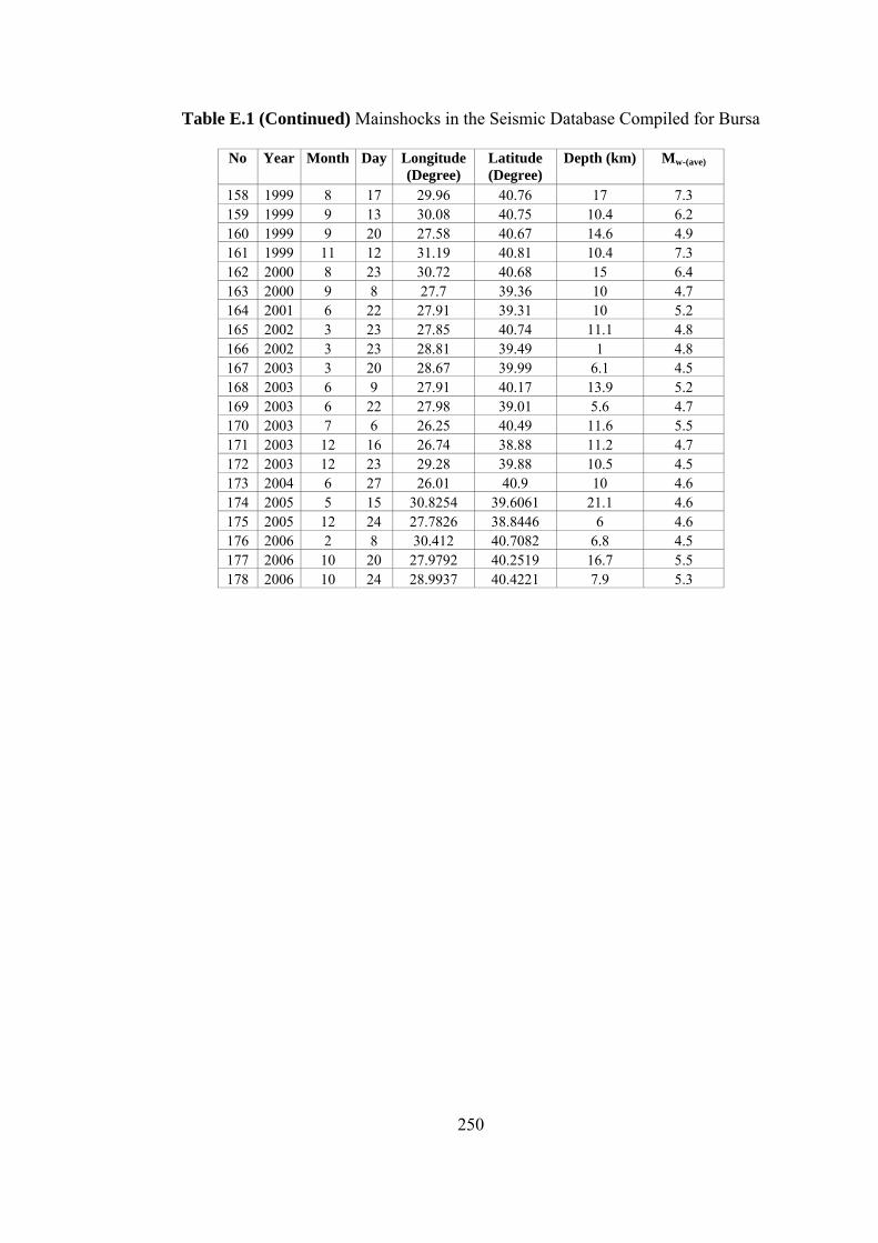
250
Table E.1 (Continued) Mainshocks in the Seismic Database Compiled for Bursa
No Year Month Day Longitude (Degree)
Latitude (Degree)
Depth (km) Mw-(ave)
158 1999 8 17 29.96 40.76 17 7.3 159 1999 9 13 30.08 40.75 10.4 6.2 160 1999 9 20 27.58 40.67 14.6 4.9 161 1999 11 12 31.19 40.81 10.4 7.3 162 2000 8 23 30.72 40.68 15 6.4 163 2000 9 8 27.7 39.36 10 4.7 164 2001 6 22 27.91 39.31 10 5.2 165 2002 3 23 27.85 40.74 11.1 4.8 166 2002 3 23 28.81 39.49 1 4.8 167 2003 3 20 28.67 39.99 6.1 4.5 168 2003 6 9 27.91 40.17 13.9 5.2 169 2003 6 22 27.98 39.01 5.6 4.7 170 2003 7 6 26.25 40.49 11.6 5.5 171 2003 12 16 26.74 38.88 11.2 4.7 172 2003 12 23 29.28 39.88 10.5 4.5 173 2004 6 27 26.01 40.9 10 4.6 174 2005 5 15 30.8254 39.6061 21.1 4.6 175 2005 12 24 27.7826 38.8446 6 4.6 176 2006 2 8 30.412 40.7082 6.8 4.5 177 2006 10 20 27.9792 40.2519 16.7 5.5 178 2006 10 24 28.9937 40.4221 7.9 5.3

251
CURRICULUM VITAE
PERSONAL INFORMATION Surname, Name: Yılmaz Öztürk, Nazan
Nationality: Turkish (TC)
Date and Place of Birth: 10 October 1976, Samsun
Phone: +90 312 287 26 80/1549
email: [email protected]
EDUCATION
Degree Institution Year of Graduation
PhD METU Civil Engineering 2008
MS METU Civil Engineering 2001
BS METU Civil Engineering 1998
High School Samsun Ondokuzmayıs High School 1993
WORK EXPERIENCE Year Place Enrollment
2006-present Earthquake Research Department, General Directorate of Disaster Affairs, Ministry of Public Works and Settlement
Civil Engineer
2005-2006 Technical Department, General Directorate of Construction Affairs, Ministry of Public Works and Settlement
Civil Engineer
1998-2005 Civil Engineering Department, Middle East Technical University
Research Assistant
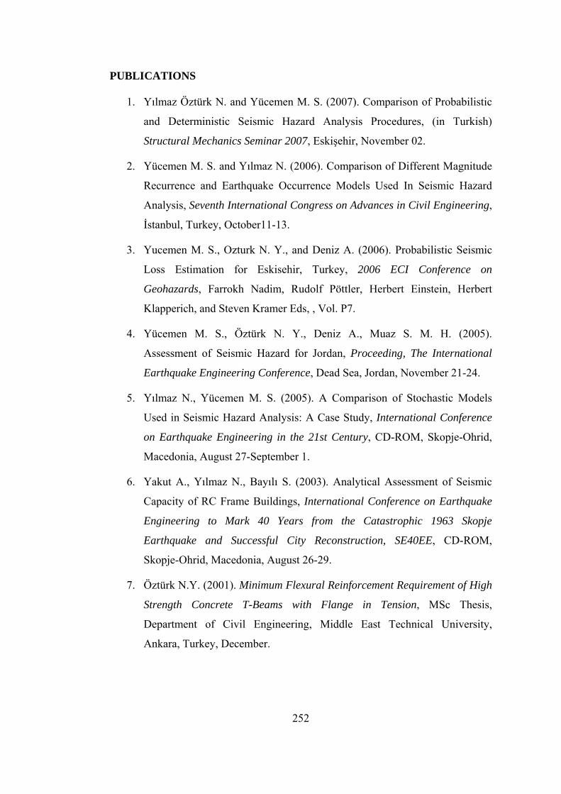
252
PUBLICATIONS
1. Yılmaz Öztürk N. and Yücemen M. S. (2007). Comparison of Probabilistic
and Deterministic Seismic Hazard Analysis Procedures, (in Turkish)
Structural Mechanics Seminar 2007, Eskişehir, November 02.
2. Yücemen M. S. and Yılmaz N. (2006). Comparison of Different Magnitude
Recurrence and Earthquake Occurrence Models Used In Seismic Hazard
Analysis, Seventh International Congress on Advances in Civil Engineering,
İstanbul, Turkey, October11-13.
3. Yucemen M. S., Ozturk N. Y., and Deniz A. (2006). Probabilistic Seismic
Loss Estimation for Eskisehir, Turkey, 2006 ECI Conference on
Geohazards, Farrokh Nadim, Rudolf Pöttler, Herbert Einstein, Herbert
Klapperich, and Steven Kramer Eds, , Vol. P7.
4. Yücemen M. S., Öztürk N. Y., Deniz A., Muaz S. M. H. (2005).
Assessment of Seismic Hazard for Jordan, Proceeding, The International
Earthquake Engineering Conference, Dead Sea, Jordan, November 21-24.
5. Yılmaz N., Yücemen M. S. (2005). A Comparison of Stochastic Models
Used in Seismic Hazard Analysis: A Case Study, International Conference
on Earthquake Engineering in the 21st Century, CD-ROM, Skopje-Ohrid,
Macedonia, August 27-September 1.
6. Yakut A., Yılmaz N., Bayılı S. (2003). Analytical Assessment of Seismic
Capacity of RC Frame Buildings, International Conference on Earthquake
Engineering to Mark 40 Years from the Catastrophic 1963 Skopje
Earthquake and Successful City Reconstruction, SE40EE, CD-ROM,
Skopje-Ohrid, Macedonia, August 26-29.
7. Öztürk N.Y. (2001). Minimum Flexural Reinforcement Requirement of High
Strength Concrete T-Beams with Flange in Tension, MSc Thesis,
Department of Civil Engineering, Middle East Technical University,
Ankara, Turkey, December.

253
8. Yılmaz N., Ersoy U., Özcebe G. (2001). Minimum Flexural Reinforcement
Requirement of High Strength Concrete T-Beams with Flange in Tension,
(in Turkish), I. Structural Mechanics Laboratories Meeting, The Scientific
and Technological Research Council of Turkey, Ankara, November.