Institute of Actuaries of Australia ABN 69 000 423 656

Level 2, 50 Carrington Street, Sydney NSW Australia 2000

t +61 (0) 2 9239 6100 f +61 (0) 2 9239 6170

e actuaries@actuaries.asn.au w www.actuaries.asn.au

Preliminary Work on the Prediction of

Extreme Rainfall Events and

Flood Events in Australia

Prepared by Kevin Fergusson

Presented to the Actuaries Institute

General Insurance Seminar

13 – 15 November 2016

Melbourne

This paper has been prepared for the Actuaries Institute 2016 General Insurance Seminar.

The Institute’s Council wishes it to be understood that opinions put forward herein are not necessarily those of the

Institute and the Council is not responsible for those opinions.

Kevin Fergusson, Centre for Actuarial Studies, University of Melbourne

The Institute will ensure that all reproductions of the paper acknowledge the

author(s) and include the above copyright statement.

Preliminary Work on the Prediction ofExtreme Rainfall Events and Flood Events

in Australia

K. FergussonCentre for Actuarial StudiesThe University of Melbourne

15th November 2016

Abstract

Among many scientific discoveries over the centuries, the pioneering work inRichardson [1922] has provided the mathematical theory of weatherforecasting used today. The subsequent technological advances of highspeed computers have allowed Richardson’s work to be exploited by modernday meteorological teams who coordinate their efforts globally to predictweather patterns on Earth, particularly extreme weather events such as floods.This paper describes preliminary work in applying some known predictors ofrainfall in Australia to forecasting extreme rainfall events and linking these toflood events.

Keywords: Floods, rainfall intensity-frequency-duration curves, sunspotnumbers, El Nino-Southern Oscillation, Southern Oscillation Index, Indian OceanDipole, Southern Annular Mode, Madden-Julian Oscillation, regression trees,bootstrapped aggregation.

1

1. Introduction

Among many scientific discoveries over the centuries, the pioneering work inRichardson [1922] has provided the mathematical theory of weatherforecasting used today. The subsequent technological advances of highspeed computers have allowed Richardson’s work to be exploited by modernday meteorological teams who coordinate their efforts globally to predictweather patterns on Earth, particularly extreme weather events such as floods.This paper describes preliminary work in applying some known predictors ofrainfall in Australia to forecasting extreme rainfall events and linking these toflood events.

2

2. Background on Australia’s Weather

A good coverage of the subject of Australia’s weather is given by Whitaker[2010], where causes of weather, measurement of weather, prediction ofweather and notable weather disasters are discussed. A fascinating history ofweather prediction and flood prediction in Australia is given in Day [2007]. Also,in Risbey et al. [2009] several drivers of rainfall, such as the Indian OceanDipole, Southern Annular Mode and Madden-Julian Oscillation, are described.In this section a background is presented on such drivers of weather as the Sun,the El Nino Southern Oscillation measured by the Southern Oscillation Index,The Indian Ocean Dipole, the Southern Annular Mode and the Madden-JulianOscillation. The aim is to employ data pertaining to these drivers to predictextreme rainfall events, which are associated with flood events.

2.1. Solar Influences of Weather on Earth

Weather on Earth is driven by the Sun’s heating of Earth, the transference of thisheat from the equator to the poles and accompanying interactions betweenoceans, the atmosphere and land masses throughout this process. Therefore,it would reasonable that the level of solar energy reaching Earth is associatedwith the level of sun spot activity, the distance of Earth from the Sun and thetilt of Earth’s axis, among other causes. For example, in Milankovic [1920], theSerbian astronomer Milankovic theorised that variations in the tilt of the earth,the precession of the earth and the eccentricity of Earth’s orbit around the Suninfluence climate on Earth. Also, the connection between the sunspot numberand solar irradiance is discussed in Boucher et al. [2001] and the connectionbetween solar cycle length and temperatures on Earth in the subsequent cycleis discussed in Solheim et al. [2012].

2.1.1. Sunspot Number

Sunspots are dark spots on the photosphere of the Sun which areconcentrations of magnetic field flux and are of relatively lower temperaturesthan their surrounds. The sunspot number has been observed for severalcenturies, waxing and waning in number, as shown in Figure 1 and is a proxy forthe level of solar inactivity.

Monthly mean total sunspot numbers, sourced from the World Data Centre -Sunspot Index and Long-Term Solar Observations (WDC-SILSO) at the RoyalObservatory of Belgium, Brussels, having the website address:

3

0

50

100

150

200

250

300

350

400

450

1700 1750 1800 1850 1900 1950 2000 2050

Sun

spo

t N

um

be

r

Year

Sunspot Numbers 1749 - 2016

Crude Sunspot Number Savitzky-Golay Filter 40,4

Figure 1: Sunspot numbers over the period 1749 to 2016

http://sidc.oma.be/silso/datafiles,

are used in the analysis. Smoothing of the data has employed the Savitzky-Golay filter, given in Savitzky and Golay [1964], with half-width 40 and degree 4polynomial. In this paper, the sunspot number is not modelled and instead theactual observed numbers are used in the predictions of extreme rainfall levels.

It is purported in Solheim et al. [2012], for example, that the length of the solarcycle is associated with lower temperatures on Earth in the subsequent solarcycle.

2.1.2. Earth’s Tilt

Earth’s tilt relative to the Sun is the angle that the Earth’s rotational axis makeswith the perpendicular to the Sun’s rays hitting the Earth. It is what causes theseasons on Earth and is a significant driver of rainfall.

It can be measured by the latitude over which the Sun is overhead, described

4

mathematically as

LSUN (d) = 23.5◦ × sin

(2π × d− 18000321

365.25

), (1)

where d is the date in YYYYMMDD format and the difference of dates iscomputed in calendar days. At the solstices the Sun is directly overhead at thenorth and south latitudes of 23.5◦, namely the Tropics of Cancer and Capricornrespectively. Also, at the equinoxes the Sun is directly overhead at the equator.It is assumed here that the Vernal Equinox occurs on the 21st of March eachyear, as is evident in (1).

2.1.3. Earth’s Distance from the Sun

A well known law of physics states that the intensity of radiation is inverselyproportional to the square of the distance from the source. This law wasdiscovered by many physicists, including Kepler, as mentioned in Gal andChen-Morris [2005], and is applicable to the intensity of solar radiation hittingthe Earth.

The distance the Earth is from the Sun can be computed from its elliptical orbitaround the Sun, given by the mathematical formula for an ellipse in polarcoordinates

rφ =A

1 + e cosφ, (2)

where e is the eccentricity of the ellipse, A is a constant. It is assumed herethat the ellipse has major and minor axes of lengths a = 149.600 million km andb = 149.579 million km respectively. The relations

a =A

1− e2, b =

A√1− e2

(3)

hold. Kepler’s second law of planetary motion states that a planet’s orbitaround its focus sweeps out a constant angular area per unit time. As anapproximation, it is assumed here that the angular speed is constant andtherefore the value of φ on day d is taken to be

φ(d) =d− 18000103

365.25× 2π, (4)

which models the Earth reaching its perihelion (closest point to the Sun, adistance of 147.1 million km) on about the 3rd of January and its aphelion(farthest point from the Sun, a distance of 152.1 million km) on about the 6th ofJuly each year.

5

The further the Earth is from the Sun, the less intense is the solar radiationreaching the Earth and therefore, the lower the energy levels associated withstorms and cyclones.

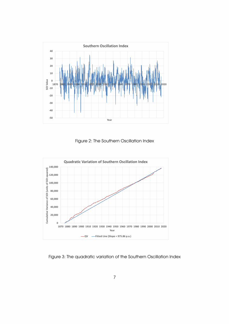
2.2. Southern Oscillation Index

The El Nino climatic event refers to a sustained warming of the tropical areas ofthe central and eastern Pacific Ocean which results in lower than averagerainfall over Eastern and Northern Australia. On the other hand, the La Ninaclimatic event refers to a sustained warming of the tropical area of the WesternPacific, which results in higher than average rainfall over Northern and EasternAustralia and potentially Central Australia. The La Nina event involves tradewinds blowing westward along the surface of the Pacific Ocean, resulting inmoisture laden air rising over the warmer area in the Western Pacific. In normalconditions, the rising air is the Western Pacific is blown eastward at higheraltitudes, leading to an air circulation known as the Walker Circulation. Thestrength of the Walker Circulation is measured by the monthly SouthernOscillation Index (SOI).

Monthly data for the SOI sourced from the Bureau of Meteorology’s website

ftp://ftp.bom.gov.au/anon/home/ncc/www/sco/soi/soiplaintext.html

for the period from 1876 to 2016 is used in the analysis and is shown in Figure2. The quadratic variation is shown in Figure 3, which shows that the volatilityof the SOI is fairly constant, demonstrating the homoskedasticity of the SOI andsimplifying the modelling of the SOI in further work.

The SOI is calculated as the difference in monthly sea level barometric pressuresat Tahiti and Darwin, adjusting for standard deviation. When the SOI maintainsa value of roughly +8 or more, it is indicative of a La Nina event. In contrast,a value of roughly −8 or less is indicative of an El Nino event, as mentioned inDavis [2012].

An example of the impact of SOI values of around −8 is when in 2010 and 2011parts of Australia experienced record-breaking rainfall, due to a La Nina event,which resulted in major flooding in South Eastern Queensland and Northern andWestern Victoria, as mentioned in Davis [2012].

6

-50

-40

-30

-20

-10

0

10

20

30

40

1870 1880 1890 1900 1910 1920 1930 1940 1950 1960 1970 1980 1990 2000 2010 2020

SOI V

alu

e

Year

Southern Oscillation Index

Figure 2: The Southern Oscillation Index

0

20,000

40,000

60,000

80,000

100,000

120,000

140,000

1870 1880 1890 1900 1910 1920 1930 1940 1950 1960 1970 1980 1990 2000 2010 2020

Cu

mu

lati

ve V

aria

nce

of

SOI (

un

its

of

SOI s

qu

are

d)

Year

Quadratic Variation of Southern Oscillation Index

QV Fitted Line (Slope = 975.86 p.a.)

Figure 3: The quadratic variation of the Southern Oscillation Index

7

2.3. Indian Ocean Dipole

The Indian Ocean Dipole (IOD) is an oscillation of warm and cold sea surfacetemperatures in the Indian Ocean and strongly influences rainfall in Australia.

Specifically, the IOD measures the difference between sea surfacetemperatures of one pole located in the Arabian Sea and another pole in theeastern Indian Ocean. Monthly data sourced from the Japan Agency forMarine-Earth Science and Technology (JAMSTEC) is used in the analysis here,the website address being

http://www.jamstec.go.jp/frcgc/research/d1/iod/DATA/dmi_HadISST.txt

and the period being from 1958 to 2010. The historical series is shown in Figure 4and the quadratic variation is shown in Figure 5. The quadratic variation of theIOD shows a periodic increase in volatility, roughly every 14 years, anddemonstrates the heteroskedasticity of the phenomenon which will need to beincorporated in the volatility process when modelling the IOD and predictingrainfall.

The three phases of the IOD are: neutral, positive and negative. In the negativephase, westerly winds blowing along the Equator allow a concentration ofwarmer water near Australia, resulting in higher than average rainfall over partsof southern Australia during Winter and Spring. The opposite happens in apositive phase, with lower than average rainfall over southern Australia.

2.4. Southern Annular Mode

The Southern Annular Mode (SAM), also known as the Antarctic Oscillation(AAO), describes the north-south movement of the westerly wind belt thatcircles Antarctica, dominating the middle to higher latitudes of the southernhemisphere.

Monthly data sourced from the website of the British Antarctic Survey,

http://www.nerc-bas.ac.uk/public/icd/gjma/newsam.1957.2007.txt,

for the period 1957 to 2016 is used in the analysis here. The historical series isshown in Figure 6 and the quadratic variation is shown in Figure 7. Thequadratic variation illustrates the periodicity of increased volatility of the SAM,roughly every 40 years. In subsequent work, the heteroskedasticity will be

8

-4

-3

-2

-1

0

1

2

3

4

1/07/1957 1/07/1967 1/07/1977 1/07/1987 1/07/1997 1/07/2007

IOD

Val

ue

Date

Indian Ocean Dipole

Figure 4: The Indian Ocean Dipole

0

10

20

30

40

50

60

70

1/07/1957 1/07/1967 1/07/1977 1/07/1987 1/07/1997 1/07/2007

QV

of

IOD

(u

nit

s o

f sq

uar

ed

IO

D u

nit

s)

Date

Quadratic Variation of the Indian Ocean Dipole

QV Fitted Line (slope = 1.32 p.a.)

Figure 5: The quadratic variation of the Indian Ocean Dipole

9

-8

-6

-4

-2

0

2

4

6

15/02/1956 14/02/1966 14/02/1976 13/02/1986 13/02/1996 12/02/2006 12/02/2016

SAM

Val

ue

Date

Southern Annular Mode 1957 - 2016

Southern Annular Mode 1Y Average 5Y Average

Figure 6: Southern Annular Mode

modelled by the SAM volatility process when determining the SAM’s influenceon rainfall.

The changing latitudinal position of this westerly wind belt affects the strengthand position of cold fronts and mid-latitude storm systems. For example, in apositive SAM event, the belt of strong westerly winds contracts towardsAntarctica, resulting in weaker westerly winds and higher pressures oversouthern Australia, thus hindering cold fronts moving inland. On the otherhand, in a negative SAM event, the belt of strong westerly winds shifts towardsthe equator, resulting in stronger storms and low pressure systems over southernAustralia and can result in southern Australia avoiding rainfall in Autumn andWinter but south eastern Australia receiving more rainfall during Spring andSummer.

2.5. Madden-Julian Oscillation

The Madden-Julian Oscillation (MJO) was discovered by Madden and Julian[1972], whereby a pulse of cloud and rainfall, called an enhanced convectivephase, and an associated suppressed convective phase, move eastward over

10

0

500

1000

1500

2000

2500

3000

3500

4000

15/02/1956 14/02/1966 14/02/1976 13/02/1986 13/02/1996 12/02/2006 12/02/2016

QV

of

SAM

(sq

uar

ed

un

its

of

SAM

)

Date

Quadratic Variation of Southern Annular Mode

QV Fitted Line (Slope 57.10 p.a.)

Figure 7: The quadratic variation of the Southern Annular Mode

the tropics with a periodicity of roughly 30 to 60 days. This dipole consisting ofthe enhanced convective phase and the suppressed convective phase moveseastward over the topics, eventually circling the globe and returning to itsoriginal position. A two-dimensional index has been developed in Wheeler andHendon [2004] which captures the MJO effect, based on combinations ofoutgoing long-wave radiation, 850-hPa zonal winds (lower altitude winds) and200-hPa zonal winds (higher altitude winds) averaged over latitudes 15◦ S to 15◦

N.

Daily data sourced from the Bureau of Meteorology’s website

http://www.bom.gov.au/climate/mjo/graphics/rmm.74toRealtime.txt

over the period 1st June 1974 to 3rd August 2016 is used in the analysis here.The two components of the MJO effect are denoted as RMM1 and RMM2 andwhen plotted on a two-dimensional graph they can be assigned a phasenumber between one and eight, according to the octant in which they lie. TheCartesian coordinates (RMM1, RMM2) can be converted to polar

11

coordinates (r, θ) using the formulae

r2 = (RMM1)2 + (RMM2)2 (5)RMM1 = r cos θ

RMM2 = r sin θ

and the phase number is determined as

1 +

{bθ − π

2π× 8c mod 8

}. (6)

The phase numbers generally correspond to locations along the Equator aroundthe globe.

A Markov Chain model applied to the time series of phases gives the transitionprobability matrix

T =

0.753 0.183 0.006 0.003 0.002 0.001 0.002 0.0480.058 0.741 0.183 0.009 0.001 0.001 0.001 0.0060.004 0.070 0.715 0.197 0.008 0.003 0.001 0.0030.002 0.004 0.046 0.765 0.170 0.007 0.003 0.0020.003 0.004 0.008 0.061 0.733 0.187 0.004 0.0010.003 0.001 0.002 0.003 0.061 0.721 0.200 0.0100.007 0.004 0.003 0.002 0.008 0.063 0.732 0.1840.194 0.007 0.002 0.001 0.003 0.005 0.058 0.730

(7)

where it is evident that transitions from Phase X mostly end up in Phase X + 1.Here the phases are 1, 2, . . . , 8 and the (i, j)-th entry of the transition probabilitymatrix T shows the probability of moving from Phase i on a given day to Phasej on the following day. So the transition matrix demonstrates that the typicalphase pattern is from 1 through all numbers to 8 and then repeating, namelythat the MJO circumscribes the Equator periodically. The transition probabilitymatrix is a useful tool for predicting future phases of the MJO given a knowledgeof its current phase, and therefore useful for rainfall prediction, as discussed inDonald [2004].

12

3. Rainfall Data

Ever since British settlement of Australia, weather data has been monitoredbecause of its relevance to agriculture and other industries. Particularly, rainfalllevels have been observed at rainfall stations located in various parts ofAustralia for more than a century.

Rainfall data sourced from the Bureau of Meteorology’s website

http://www.bom.gov.au/watl/rainfall/observations/

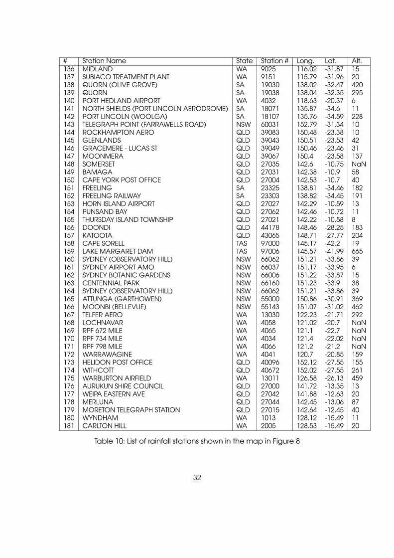
is used in the analysis here. The 181 locations of the rainfall stations used in theanalysis are shown in Figure 8 and in Appendix B.

-45

-40

-35

-30

-25

-20

-15

-10

110 115 120 125 130 135 140 145 150 155 160De

gre

es

Lati

tud

e (

Ne

gati

ve In

dic

ate

s So

uth

)

Degrees Longitude East

Australian Rainfall Station Locations

Figure 8: Location of rainfall stations in Australia

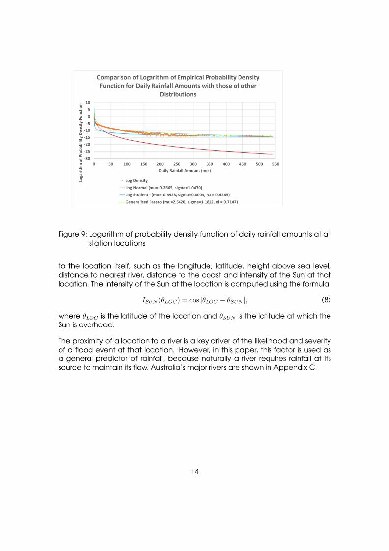
The logarithm of the probability density function of daily rainfall amounts inshown in Figure 9. Taking the logarithm allows a comparison to be made withother distributions in the tails of the distributions. It is evident that a GeneralisedPareto distribution provides a good fit to the distribution of observed rainfallamounts, which is to be used in subsequent research.

Based on the available data, several predictive factors in Appendix A pertain

13

‐30‐25‐20‐15‐10‐50510

0 50 100 150 200 250 300 350 400 450 500 550

Logarithm

 of P

roba

bility Den

sity Fun

ction

Daily Rainfall Amount (mm)

Comparison of Logarithm of Empirical Probability Density Function for Daily Rainfall Amounts with those of other 

Distributions

Log Density

Log Normal (mu=‐0.2665, sigma=1.0470)

Log Student t (mu=‐0.6928, sigma=0.0003, nu = 0.4265)

Generalised Pareto (mu=2.5420, sigma=1.1812, xi = 0.7147)

Figure 9: Logarithm of probability density function of daily rainfall amounts at allstation locations

to the location itself, such as the longitude, latitude, height above sea level,distance to nearest river, distance to the coast and intensity of the Sun at thatlocation. The intensity of the Sun at the location is computed using the formula

ISUN (θLOC) = cos |θLOC − θSUN |, (8)

where θLOC is the latitude of the location and θSUN is the latitude at which theSun is overhead.

The proximity of a location to a river is a key driver of the likelihood and severityof a flood event at that location. However, in this paper, this factor is used asa general predictor of rainfall, because naturally a river requires rainfall at itssource to maintain its flow. Australia’s major rivers are shown in Appendix C.

14

4. Flood Event Data

Floods in Australia are typically associated with either tropical cyclones, forexample in the the northern areas of Australia, or slow moving low pressurecells, such as in southern areas of Australia. There are other pertinent factorsassociated with floods, such as the topography of the location, proximity torivers, heights of river banks and hydrology of the location. So, it would be idealto have river gauge data for the major rivers shown in Appendix C,topographical data and hydrological data to determine precisely howextreme rainfall events lead to flood events. However, in this paper, rainfalllevels which correspond to flood events are deduced by looking at thefollowing historical flood events, sourced from Whitaker [2010] and Davis [2012]:

• Brisbane, 1839 - the gauge height of the Brisbane River at the Post Officewas about 8.4m;

• Brisbane, March 1890 - the gauge height of the Brisbane River at the PostOffice was about 5.3m;

• Brisbane, February 1893 - the gauge height of the Brisbane River at the PostOffice was about 8.4m;

• Northern Tasmania, April 1929 - an intense slow moving low pressure cellover central Victoria brought heavy rainfall;

• Hunter Valley, February 1955 - a low pressure cell over north-eastern NewSouth Wales brought heavy rainfall;

• Brisbane, January 1974 - Tropical Cyclone Wanda dumped heavy rainfallacross Brisbane, causing major flooding of the Brisbane River, resulting in itshighest gauge reading for the century;

• Brisbane, January 2011 - heavy intense rainfall resulted in floods, with thegauge height of the Brisbane River at the Post Office being about 4.5m;

• Katherine, December 2011 - Tropical Cyclone Grant brought heavy rainfallwhich caused floods north of Katherine;

Flood peak data for Brisbane is shown in Figure 10 and rainfall amounts duringflood events are shown in Table 1, which corroborate some of theaforementioned flood events. Each flood event has involved at least one dayof rainfall of around 90 mm or more.

15

Flood Event Rf Stn Day 1 Day 2 Day 3 Day 4Northern Tasmania 19290403 19290404 19290405 19290406(April 1929) YOLLA 6.1 mm 114.3 mm 101.6 mm 83.8 mmHunter Valley 19550223 19550224 19550225 19550226(February 1955) NEWC 0 mm 83.8 mm 24.6 mm 40.1 mm

ATTU 22.9 mm 38.9 mm 89.4 mm 109 mmBrisbane 19740125 19740126 19740127 19740128( January 1974) TOOW 104.6 mm

ALDE 62 mm 224 mm 220 mm 43 mmBrisbane 20110109 20110110 20110111 20110112(January 2011) ALDE 23.4 mm 123.2 mm 28.2 mm 54.2 mm

MT MEE 64.6 mm 189.6 mm 185 mm 176 mmKatherine 20111225 20111226 20111227 20111228(December 2011) KATH 0 mm 0 mm 255 mm 1 mm

KOOL 143 mm 0 mm

Table 1: Daily rainfall amounts during various historical flood events at rainfallstations listed in Table 2

Abbreviation Rainfall Station DetailsYOLLA YOLLA (SEA VIEW) (TAS) Lat -41.14 Long 145.71NEWC NEWCASTLE NOBBYS SIGNAL STATION AWS (NSW) Lat -32.9 Long 152ATTU ATTUNGA (GARTHOWEN) (NSW) Lat -30.9 Long 151TOOW TOOWONG BOWLS CLUB (QLD) Lat -27.5 Long 153ALDE ALDERLEY (QLD) Lat -27.4 Long 153ALDE ALDERLEY (QLD) Lat -27.4 Long 153MT MEE MT MEE (QLD) Lat -27.1 Long 153KATH CDU KATHERINE RURAL CAMPUS (NT) Lat -14.37 Long 132.16KOOL KOOLPINYAH (NT) Lat -12.4 Long 131

Table 2: List of details of rainfall stations corresponding to various flood events

16

Figure 10: Highest annual flood peaks for Brisbane (source: BOM, withpermission)

17

5. Methodology

The aim here is to predict flood events by using a combination of weatherindices such as IOD, SAM, MJO and SOI and solar indicators.

Extreme rainfall events are characterised here by n-day rainfall intensities inexcess of a 90 mm per day threshold, for n = 1, 2, 3, 4, 5. These levels roughlycorrespond to flood events in Brisbane and other cities.

The predictive factors which are best able to identify extreme rainfall events,out-of-sample, using regression trees, as described by Berk [2008] aredetermined. The in-sample data set for the analysis covers the period from 1stJanuary 1800 to 31st December 1989. The out-of-sample period is from 1stJanuary 1990 to 30th June 2016. An explanation of regression trees andbootstrapped aggregation of regression trees is provided here by first lookingat ordinary least squares regression.

5.1. Ordinary Least Squares Regression

Given the independent data matrix X and the dependent data vector Y it issought to predict the values of Y using the data matrix X. Here X is an n × pmatrix and Y is an n× 1 matrix, or equivalently a column vector of length n. Thevalue of n is the number of data points observed and for the in-sample data setn = 1, 108, 286. The value of p is the number of predictors in Table 9 in AppendixA, that is n = 23. The (i, j)-th entry of X, denoted by Xi,j , corresponds to thei-th data observation of the j-th independent variable or predictor variable.For example, X2,1 is the second observation of the sunspot number. Also thei-th entry of Y , denoted by Yi, corresponds to the i-th data observation of theresponse variable, namely the i-th rainfall observation.

Ordinary Least Squares Regression (OLS) models the response variable, which isthe daily rainfall amount, as a constant term β0 plus a linear combination of thepredictor variables, that is

Yi = β0 + β1Xi,1 + . . .+ βpXi,p + εi, (9)

where the sum of the squares of the error terms εi is minimised. In matrix notation,the equation can be written as

Y = [1˜|X]β˜ + ε˜, (10)

where 1˜ is a column vector of ones of length n, β˜ = (β0, . . . , βp)T and

ε˜ = (ε1, . . . εn)T . A statistical measure of the explanatory power of the model is

18

Statistic 1D 2D 3D 4D 5DR-squ (in-sample) 8.2% 12.1% 15.3% 18.2% 20.8%R-squ (out-of-sample) 7.5% 10.4% 13.1% 15.4% 17.6%R-squ (out-of-sample for -10.2% -18.6% -28.7% -36.9% -46.0%predicted RF≥15mm)

Table 3: R-squared statistics of the OLS regression fits

given by the R-squared statistic, which is calculated using the formula

R2 = 1− V AR(ε˜)V AR(Y )

, (11)

where

V AR(Y ) =1

n

n∑i=1

(Yi − E(Y )

)2 (12)

is the variance of Y and V AR(ε˜) is the variance of ε. The R-squared statistics ofOLS regression fits are shown in Table 3. It is clear that the ability of the OLSregression model to predict daily rainfall levels out-of-sample is poor and itsability to predict rainfall intensities over higher durations is better, due toaggregate rainfall statistics being less volatile. However, the OLS regressionmodel is incapable of predicting rainfall intensities in excess of 15mm per day,for any duration, let alone rainfall intensities in excess of 90mm per day as washoped. The problem with predicting 90mm or more of rainfall is that the OLSmodel fails to predict any such levels out of sample, and therefore noR-squared statistic can be calculated.

The OLS regression when performed on quantiles of the predictor variablesgives normalised coefficients, shown in Table 4, whose magnitudes indicate theimportance of the predictor variables. Based on this, the top four predictorvariables in order of importance are:

• Average daily rainfall over previous years in that month at location;

• Intensity of Sun at rainfall station;

• Latitude of rainfall station;

• Standard deviation of daily rainfall over previous years in that month atlocation;

for each of the durations of one to five days. The following remarks arepertinent. The intensity of the Sun at a location with latitude θLOC is given by (8)and this intensity varies with the latitude θSUN at which the Sun is overhead. Forlocations in Australia, the intensity of the Sun is a maximum when

19

Factor 1D 2D 3D 4D 5DConstant unity 2.9129 2.8307 2.7784 2.7178 2.6570Sunspot number 0.4524 0.4643 0.4716 0.4717 0.4796SG filter 0.4785 0.4751 0.4728 0.4669 0.4685Time in current SS cycle 0.4840 0.4348 0.4247 0.4147 0.4065Lat. Sun overhead 2.4794 2.4536 2.5015 2.5856 2.7049Time in current tilt cycle 0.8009 0.7701 0.7551 0.7599 0.7759Distance from Sun 1.5227 1.4678 1.5015 1.5746 1.6861Time in current orbital period 0.9854 0.9756 0.9746 0.9668 0.9581SOI 1.0982 1.0804 1.0630 1.0464 1.0340IOD 0.0680 0.0833 0.0909 0.0977 0.1030SAM 0.3260 0.3161 0.3124 0.3069 0.3020MJO: RMM1 0.4692 0.5111 0.5392 0.5620 0.5802MJO: RMM2 1.2216 1.2132 1.1653 1.0974 0.9963MJO: r 0.0475 0.0517 0.0570 0.0618 0.0661MJO: theta 0.1480 0.1776 0.2009 0.2166 0.2277MJO: phase 0.2271 0.2946 0.3058 0.2991 0.2542Long. of RF stn. 0.1131 0.1282 0.1273 0.1257 0.1242Lat. of RF stn. 5.4938 4.6366 4.4322 4.2790 4.1548RF stn. hgt. above SL 0.0159 0.0410 0.0600 0.0790 0.0972Distance RF stn. from river 0.0287 0.0002 0.0142 0.0248 0.0349Distance RF stn. from coast 0.1930 0.1443 0.1245 0.1080 0.0931Intensity of Sun 8.4262 7.5314 7.2902 7.1061 6.9542Avg. daily RF for month 10.1640 9.9415 9.8200 9.7333 9.6585Std. dev. daily RF for month 3.8977 3.8312 3.7797 3.7425 3.7115

Table 4: Regression coefficients for various durations

θSUN = max{−23.5◦, θLOC}, which roughly corresponds to Australia’s Summer. Incontrast, the latitude of the rainfall station is, for a given rainfall station, fixed. Sothe intensity of the Sun is a proxy for the closeness of the season to Summer,concurring with the tropical wet season in northern Australia, and the latitudeof the rainfall station is simply a measure of distance to the Equator. The tworemaining predictor variables, the average daily rainfall and the standarddeviation of daily rainfall, are obvious indicators of daily rainfall levels and areonly associated to the extent that higher average daily rainfall correlates witha higher standard deviation of daily rainfall. The rationale for including both aspredictive factors, despite their potential correlation, is that, ignoring thirdorder and higher moments, the daily rainfall is approximately the sum of theaverage daily rainfall and a noise term which is the product of the standarddeviation of daily rainfall and a normalised random variable, that is one havingmean zero and variance one.

20

5.2. Regression Trees

The simplest regression tree consists of a decision node and two emanatingbranches. The decision node involves the choice of a factor, say the i1-th, anda demarcation value, say θ1, such that the partitioned response variables areas homogeneous as possible. Mathematically, the variables i1 and θ1 arechosen such that∑

i∈{k:Xk,i1≤θ1}

(Yi − E[Yj |Xj,i1 ≤ θ1])2 +∑

i∈{k:Xk,i1>θ1}

(Yi − E[Yj |Xj,i1 > θ1])2 (13)

is minimised, where i1 ∈ {1, 2, . . . , p}, θ1 ∈ (−∞,∞) and

E[Yj |Xj,i1 ≤ θ1] ={ ∑j∈{k:Xk,i1

≤θ1}

Yj

}/|{k : Xk,i1 ≤ θ1}| (14)

E[Yj |Xj,i1 > θ1] =

{ ∑j∈{k:Xk,i1

>θ1}

Yj

}/|{k : Xk,i1 > θ1}|. (15)

This procedure can be extended to each branch’s partition of the data set toform another two nodes each of which has two emanating branches, resultingin a tree with three nodes and six branches. Recursive application of thisprocedure can be continued until a desired level of fit has been achieved oruntil a prespecified maximum number of nodes is reached. Given a set ofpredictor variables, the predicted response variable is simply the average ofthe response variables in the partition at the base of the tree corresponding tothe sequence of decisions taken at preceding nodes.

The R-squared statistics of the regression tree fits having 100 nodes (or splits) areshown in Table 5. It is clear that the ability of the model to predict daily rainfalllevels out-of-sample is poor and its ability to predict rainfall intensities overhigher durations is better, due to aggregate rainfall statistics being less volatile.Comparison of Table 5 with Table 3 indicates that the out-of-sampleperformance of the regression tree model is inferior to that of the OLSregression model, despite its better in-sample fit. However, unlike the OLSregression model, the regression tree model is able to provide predictions ofrainfall intensities in excess of 75mm per day and 90mm per day, for a two-dayduration, as is evident in Table 5.

The R-squared statistics for regression tree models having 50,000 nodes areshown in Table 6, where the high R-squared statistics of in-sample performancescontrast with the lowly valued statistics for the out-of-sample performances andis symptomatic of overfitting. We overcome this drawback in the next section.

21

Statistic 1D 2D 3D 4D 5DR-squ (in-sample) 11.2% 16.1% 19.7% 22.9% 26.0%R-squ (out-of-sample) 2.6% -13.3% 12.6% 14.1% 16.7%R-squ (out-of-sample -39.7% -172.8% -7.9% -20.8% -15.7%for predicted RF≥15mm)R-squ (out-of-sample -112.9% -400.5% -1033.2% -327.5% -346.7%for predicted RF≥30mm)R-squ (out-of-sample -294.2% -66.8% 0.0% -65.5% -73.6%for predicted RF≥45mm)R-squ (out-of-sample -179.7% -66.8% 0.0% 0.0% 0.0%for predicted RF≥60mm)R-squ (out-of-sample -179.7% 0.3% 0.0% -100.0% -100.0%for predicted RF≥75mm)R-squ (out-of-sample -110.7% 0.3% -100.0% -100.0% -100.0%for predicted RF≥90mm)

Table 5: R-squared statistics of the regression tree fits with 100 splits

Statistic 1D 2D 3D 4D 5DR-squ (in-sample) 68.8% 78.7% 83.6% 87.4% 89.7%R-squ (out-of-sample) -121.6% -121.3% -113.0% -86.1% -83.6%R-squ (out-of-sample -328.6% -242.0% -230.8% -183.7% -152.8%for predicted RF≥15mm)R-squ (out-of-sample -426.9% -289.1% -301.9% -228.7% -154.2%for predicted RF≥30mm)R-squ (out-of-sample -639.3% -364.4% -233.6% -242.3% -130.8%for predicted RF≥45mm)R-squ (out-of-sample -863.1% -383.9% -227.6% -361.6% -124.4%for predicted RF≥60mm)R-squ (out-of-sample -1056.5% -350.8% -205.7% -488.4% -171.6%for predicted RF≥75mm)R-squ (out-of-sample -1558.4% -384.5% -212.6% -553.2% -1261.2%for predicted RF≥90mm)

Table 6: R-squared statistics of the regression tree fits with 50,000 splits

22

5.3. Bootstrapped Aggregation of Regression Trees (BAGGING)

A drawback of the regression tree approach is that it can overfit the data andtherefore perform poorly out-of-sample. To overcome this, a modified data setcan be constructed by sampling with replacement from the original data set,known as bootstrapping, and then a resulting regression tree can be built fromthis modified data set. As many trees as desired can be built in this fashion,allowing one to calculate a consensus prediction from the built trees. This isknown as bootstrapped aggregation of regression trees, due to Breiman [1996],and is commonly called BAGGING.

The BAGGING model is applied to predicting rainfall intensities over durations ofone to five days, with the results using 200 nodes and 40 trees shown in Table7. The out-of-sample R-squared statistics are higher than those of the OLS andregression tree models.

By increasing the number of nodes to 50,000 and the number of trees to 200,the regression trees are better able to fit the data in-sample, particularly theextreme values, as shown in Table 8. As suggested by the positive R-squaredstatistic, BAGGING can predict rainfall intensities in excess of 15mm per day fora three-day duration and of 45mm per day for a five-day duration, but mostlyits out-of-sample performance is poor. It is likely that many more trees arerequired to ameliorate this deficiency, which will demand a significant increasein the level of computing power than that used here, and will be investigatedin subsequent work on the subject.

23

Statistic 1D 2D 3D 4D 5DR-squ (in-sample) 14.1% 19.1% 23.8% 27.4% 30.2%R-squ (out-of-sample) 8.1% 11.6% 15.1% 18.1% 20.9%R-squ (out-of sample -2.1% -2.6% -0.4% -1.1% -1.6%for predicted RF≥15mm)R-squ (out-of sample -32.2% -12.6% -10.2% N/A -563.1%for predicted RF≥30mm)R-squ (out-of sample -22168.5% N/A N/A N/A N/Afor predicted RF≥45mm)R-squ (out-of sample -22168.5% N/A N/A N/A N/Afor predicted RF≥60mm)R-squ (out-of sample -22168.5% N/A N/A N/A N/Afor predicted RF≥75mm)R-squ (out-of sample N/A N/A N/A N/A N/Afor predicted RF≥90mm)

Table 7: R-squared statistics of the bootstrapped aggregation of regression treefits using 200 splits and 40 trees

Statistic 1D 2D 3D 4D 5DR-squ (in-sample) 65.6% 78.3% 84.3% 88.1% 90.6%R-squ (out-of-sample) 4.9% 8.3% 11.5% 14.8% 17.4%R-squ (out-of sample -2.3% -1.2% 0.1% -0.6% -0.4%for predicted RF≥15mm)R-squ (out-of sample -3.7% -3.3% -4.8% -0.9% -5.3%for predicted RF≥30mm)R-squ (out-of sample -3.9% -4.8% -5.7% -44.6% 52.3%for predicted RF≥45mm)R-squ (out-of sample -15.0% -22.0% N/A N/A N/Afor predicted RF≥60mm)R-squ (out-of sample -1454.6% N/A N/A N/A N/Afor predicted RF≥75mm)R-squ (out-of sample N/A N/A N/A N/A N/Afor predicted RF≥90mm)

Table 8: R-squared statistics of the bootstrapped aggregation of regression treefits using 50,000 splits and 200 trees

24

6. Conclusions

It has been shown how bootstrapped aggregation of regression trees canprovide better prediction of extreme rainfall events out-of-sample than OLSand single regression tree models. Increasing the number of splits in theregression tree models allows adherence of the model to in-sample data andincreasing the number of trees beyond 200 in the aggregated regression treemodel in Section 5.3, will potentially give reliable out-of-sample predictions ofrainfall intensities of 90mm or more and flood events. This will entail the use ofgreater computing power than used here.

What is apparent from the R-squared statistics is that the prediction powers ofthe models are higher for rainfall intensities of five days’ duration than for shorterdurations. Clearly, it is the high intensity rainfall events over short durations whichcause most floods and therefore there is much improvement to be done on theanalysis here.

Another point is that no matter how good the model, if there is little informationcontent in the data then the predictive power of the model will be low. Thus,additional improvements to the modelling can be made by incorporatingadditional data such as temperature data, air pressure data, river gaugereadings, hydrological maps and topographical maps. Subsequent work willincorporate such additional data as well as spatial models such as thosedescribed in Gschlössl [2006] and Lehmann et al. [2015].

25

References

R. A. Berk. Statistical Learning from a Regression Perspective. Springer, 2008.

O. Boucher, J. Haigh, D. Hauglustaine, J. Haywood, G. Myhre, T. Nakajima, G.Y.Shi, and S. Solomon. Radiative forcing of climate change. In Climate Change2001: The Scientific Basis, pages 351–416. Intergovernmental Panel on ClimateChange, 2001.

L. Breiman. Bagging predictors. Machine Learning, 24(2):123–140, 1996.

S. Davis. Record-breaking La Nina events. http://www.bom.gov.au/climate/enso/history/La-Nina-2010-12.pdf, July 2012.

D. Day. The Weather Watchers: 100 Years of the Bureau of Meteorology.Melbourne University Publishing, 2007.

A. Donald. Australian rainfall and the MJO. The Australian Cotton Grower, pages40–42, April-May 2004.

O. Gal and R. Chen-Morris. The archaeology of the inverse square law:Metaphysical images and mathematical practices. History of Science, 43:391–414, 2005.

S. Gschlössl. Hierarchical bayesian spatial regression models with applicationsto non-life insurance. Doctoral dissertation, Technische Universität München,2006.

E.A. Lehmann, A. Phatak, A. Stephenson, and R. Lau. Spatial modellingframework for the characterisation of rainfall extremes at different durationsand under climate change. Environmetrics, 27(4):239–251, 2015.

R. A. Madden and P. R. Julian. Description of global-scale circulation cells in thetropics with a 40-50 day period. Journal of Atmospheric Science, 29:1109–1123, 1972.

M. Milankovic. Theorie Mathematique des Phenomenes Thermiques produitspar la Radiation Solaire. Gauthier-Villars Paris, 1920.

L. F. Richardson. Weather Prediction by Numerical Process. Cambridge, TheUniversity press, 1922.

J.S. Risbey, M.J. Pook, P.C. Mclntosh, M.C. Wheeler, and H.H. Hendon. On theremote drivers of rainfall variability in Australia. American MeteorologicalSociety Monthly Weather Review, 137(10):3233–3253, 2009.

A. Savitzky and M.J.E. Golay. Smoothing and differentiation of data by simplifiedleast squares procedures. Analytical Chemistry, 36(8):1627–1639, 1964.

26

J. Solheim, K. Stordahl, and O. Humlum. The long sunspot cycle 23 predicts asignificant temperature decrease in cycle 24. Journal of Atmospheric andSolar-Terrestrial Physics, 80:267–284, 2012.

M.C. Wheeler and H.H. Hendon. An all-season real-time multivariate MJOindex: Development of an index for monitoring and prediction. AmericanMeteorological Society Monthly Weather Review, 132(8):1917–1932, 2004.

R. Whitaker. The Complete Book of Australian Weather. Allen and Unwin, 2010.

27

A. List of Predictive Factors

# Predictive Factor1 Sunspot number2 SG Filter of sunspot number3 Proportion of time in current sunspot cycle4 Latitude at which Sun is overhead5 Proportion of time in current tilt cycle6 Distance from Sun7 Proportion of time in current orbital period8 Southern Oscillation Index9 Indian Ocean Dipole10 Southern Annular Mode11 Madden-Julian Oscillation: RMM112 Madden-Julian Oscillation: RMM213 Madden-Julian Oscillation: r14 Madden-Julian Oscillation: theta15 Madden-Julian Oscillation: phase16 Longitude of rainfall station17 Latitude of rainfall station18 Rainfall station’s height above sea level19 Distance rainfall station from nearest major river20 Distance rainfall station from coast21 Intensity of Sun at rainfall station22 Average daily rainfall over previous years in that month at location23 Standard deviation of daily rainfall over previous years in that month at location

Table 9: List of predictive factors for rainfall levels

28

B. List of Rainfall Stations

# Station Name State Station # Long. Lat. Alt.1 NORTH ADELAIDE SA 23011 138.6 -34.92 482 ADELAIDE AIRPORT SA 23034 138.52 -34.95 23 ADELAIDE (GLEN OSMOND) SA 23005 138.65 -34.95 1284 ADELAIDE (MORPHETTVILLE RACECOURSE) SA 23098 138.54 -34.97 115 NORTH ADELAIDE SA 23011 138.6 -34.92 486 ALBANY WA 9500 117.88 -35.03 37 ALICE SPRINGS AIRPORT NT 15590 133.89 -23.8 5468 BOND SPRINGS HOMESTEAD NT 15631 133.92 -23.54 7649 CAPE LEEUWIN WA 9518 115.14 -34.37 1310 FOREST GROVE WA 9547 115.08 -34.07 6011 BALLARAT AERODROME VIC 89002 143.79 -37.51 43512 BUNGAREE (KIRKS RESERVOIR) VIC 87014 143.93 -37.55 51113 RAYWOOD VIC 81041 144.21 -36.53 12714 CLIFTON HILLS SA 17016 138.89 -27.02 3215 BIRDSVILLE POLICE STATION QLD 38002 139.35 -25.9 3716 ROSEBERTH STATION QLD 38020 139.59 -25.79 4717 BORROLOOLA NT 14710 136.3 -16.07 1718 BORROLOOLA AIRPORT NT 14723 136.3 -16.08 1619 CENTRE ISLAND NT 14703 136.82 -15.74 1220 MCARTHUR RIVER MINE AIRPORT NT 14704 136.08 -16.44 4021 BOULIA AIRPORT QLD 38003 139.9 -22.91 16222 ELROSE STATION QLD 37103 140.11 -22.82 10823 MARION DOWNS QLD 38014 139.66 -23.37 12424 COLLERINA (KENEBREE) NSW 48052 146.52 -29.77 10725 FORDS BRIDGE (DELTA) NSW 48194 145.29 -30.08 11126 TOOWONG BOWLS CLUB QLD 40245 152.99 -27.49 1027 ALDERLEY QLD 40224 153 -27.42 3928 BROKEN HILL (PATTON STREET) NSW 47007 141.47 -31.98 31529 BROKEN HILL AIRPORT AWS NSW 47048 141.47 -32 28130 BROKEN HILL (STEPHENS CREEK RESERVOIR) NSW 47031 141.59 -31.88 23831 BROOME AIRPORT WA 3003 122.24 -17.95 732 BIDYADANGA WA 3030 121.78 -18.68 1133 ROEBUCK PLAINS WA 3023 122.47 -17.93 1534 FAIRYMEAD SUGAR MILL QLD 39037 152.36 -24.79 535 DAYBORO POST OFFICE QLD 40063 152.82 -27.2 6836 MT MEE QLD 40145 152.78 -27.06 46537 WAMURAN QLD 40343 152.87 -27.04 3338 CAIRNS AERO QLD 31011 145.75 -16.87 239 KURANDA RAILWAY STATION QLD 31036 145.64 -16.82 34040 MULGRAVE MILL QLD 31049 145.79 -17.09 1541 AINSLIE TYSON ST NSW 70000 149.14 -35.26 58542 CARNARVON AIRPORT WA 6011 113.67 -24.89 443 BOOLATHANA WA 6003 113.69 -24.65 444 BRICKHOUSE WA 6005 113.79 -24.82 1545 AUGUSTUS DOWNS STATION QLD 29001 139.87 -18.54 75

29

# Station Name State Station # Long. Lat. Alt.46 BURKETOWN POST OFFICE QLD 29004 139.55 -17.74 647 COBAR (DOUBLE GATES) NSW 48034 145.48 -31.69 17548 COBAR MO NSW 48027 145.83 -31.48 26049 COBAR (TINDAREY) NSW 48075 145.83 -31.12 19050 COOBER PEDY SA 16007 134.76 -29 21551 COOBER PEDY (MCDOUALL PEAK) SA 16027 134.9 -29.84 15052 COOLGARDIE WA 12018 121.17 -30.96 42753 MALLINA WA 4059 118.03 -20.88 4054 DAMPIER SALT WA 5061 116.75 -20.73 655 DARWIN AIRPORT NT 14015 130.89 -12.42 3056 DERBY AERO WA 3032 123.66 -17.37 657 YEEDA WA 3026 123.65 -17.62 558 EDEN (TIMBILLICA) NSW 69029 149.7 -37.36 3559 ELLIOTT NT 15131 133.54 -17.56 22060 ESPERANCE DOWNS RESEARCH STN WA 9631 121.78 -33.6 15861 MYRUP WA 9584 122 -33.74 6062 EUCLA WA 11003 128.9 -31.68 9363 MUNDRABILLA STATION WA 11008 127.86 -31.84 2064 EXMOUTH GULF WA 5004 114.11 -22.38 1565 LEARMONTH AIRPORT WA 5007 114.1 -22.24 566 EXMOUTH TOWN WA 5051 114.13 -21.93 1367 YANREY WA 5030 114.79 -22.51 2568 FITZROY CROSSING AERO WA 3093 125.56 -18.18 11569 FOSSIL DOWNS WA 3027 125.78 -18.14 12070 GOGO STATION WA 3014 125.59 -18.29 15071 GERALDTON TOWN WA 8050 114.61 -28.78 372 HOWATHARRA WA 8168 114.62 -28.55 7073 NABAWA WA 8028 114.79 -28.5 14574 NORTHAMPTON WA 8100 114.64 -28.35 18075 SANDSPRINGS WA 8116 114.94 -28.79 22076 BALGO HILLS WA 13007 127.99 -20.14 42077 GILES METEOROLOGICAL OFFICE WA 13017 128.3 -25.03 59878 GOVE AIRPORT NT 14508 136.82 -12.27 5279 ALCAN MINESITE NT 14509 136.84 -12.26 2080 BINYA POST OFFICE NSW 75006 146.34 -34.23 14181 WHITTON (CONAPAIRA ST) NSW 74118 146.18 -34.51 13282 YENDA (HENRY STREET) NSW 75079 146.19 -34.25 12983 HALLS CREEK AIRPORT WA 2012 127.66 -18.23 42284 MOOLA BULLA WA 2020 127.5 -18.19 43085 HOBART BOTANICAL GARDENS TAS 94030 147.33 -42.87 2786 HOBART (ELLERSLIE ROAD) TAS 94029 147.33 -42.89 5187 HOWARD SPRINGS NATURE PARK NT 14149 131.05 -12.46 3488 KOOLPINYAH NT 14032 131.18 -12.39 3089 MIDDLE POINT RANGERS NT 14090 131.31 -12.58 1090 NAPPA MERRIE QLD 45012 141.11 -27.6 66

30

# Station Name State Station # Long. Lat. Alt.91 INNAMINCKA STATION SA 17028 140.76 -27.72 5392 KALGOORLIE-BOULDER AIRPORT WA 12038 121.45 -30.78 36593 BULONG WA 12013 121.75 -30.75 38094 KARRATHA STATION WA 5052 116.67 -20.88 3095 LAUNCESTON (DISTILLERY CREEK) TAS 91181 147.21 -41.43 12096 LAUNCESTON (KINGS MEADOWS) TAS 91072 147.16 -41.47 6797 COEN AIRPORT EVAP QLD 27006 143.12 -13.76 16198 MEIN STATION QLD 27014 142.8 -13.18 12299 LOCKHART RIVER AIRPORT QLD 28008 143.3 -12.79 19100 LONGREACH AERO QLD 36031 144.28 -23.44 192101 BEACONSFIELD QLD 36066 144.6 -23.33 230102 CAMOOLA PARK QLD 36013 144.52 -23.04 188103 EVESHAM STATION QLD 36022 143.71 -23.03 190104 SUMMER HILL QLD 36153 144.81 -23.05 240105 WHITEHILL QLD 36131 144.05 -23.64 210106 FARLEIGH CO-OP SUGAR MILL QLD 33023 149.1 -21.1 47107 MACKAY M.O QLD 33119 149.22 -21.12 30108 PLEYSTOWE SUGAR MILL QLD 33060 149.04 -21.14 27109 GABO ISLAND LIGHTHOUSE VIC 84016 149.92 -37.57 15110 FLEMINGTON RACECOURSE VIC 86039 144.91 -37.79 10111 CAULFIELD (RACECOURSE) VIC 86018 145.04 -37.88 49112 FLEMINGTON RACECOURSE VIC 86039 144.91 -37.79 10113 OAKLEIGH (METROPOLITAN GOLF CLUB) VIC 86088 145.09 -37.91 61114 CALTON HILLS STATION QLD 29118 139.41 -20.14 350115 WEST LEICHHARDT STATION QLD 29121 139.69 -20.6 280116 MOUNT ISA MINE QLD 29126 139.48 -20.74 381117 OBAN STATION QLD 37035 139.05 -21.23 282118 NANNUP WA 9585 115.77 -33.98 100119 NEWCASTLE NOBBYS SIGNAL STATION AWS NSW 61055 151.8 -32.92 33120 NEWCASTLE WATERS NT 15086 133.41 -17.38 209121 WILLIAMTOWN RAAF NSW 61078 151.84 -32.79 9122 NHULUNBUY NT 14512 136.76 -12.19 20123 NORMANTON AIRPORT QLD 29063 141.07 -17.69 18124 NORMANTON HOSPITAL QLD 29073 141.08 -17.68 12125 NORMANTON POST OFFICE QLD 29041 141.07 -17.67 8126 I DUNNO WA 12077 121.71 -32.86 270127 SALMON GUMS RES.STN. WA 12071 121.62 -32.99 249128 OODNADATTA AIRPORT SA 17043 135.45 -27.56 117129 HAMILTON STATION SA 16083 135.08 -26.71 170130 PARABURDOO AERO WA 7185 117.75 -23.17 424131 ASHBURTON DOWNS WA 7119 117.03 -23.39 250132 PARDOO STATION WA 4028 119.58 -20.11 9133 PERTH AIRPORT WA 9021 115.98 -31.93 15134 PERTH AIRPORT WA 9021 115.98 -31.93 15135 GOSNELLS CITY WA 9106 115.98 -32.05 10

31

# Station Name State Station # Long. Lat. Alt.136 MIDLAND WA 9025 116.02 -31.87 15137 SUBIACO TREATMENT PLANT WA 9151 115.79 -31.96 20138 QUORN (OLIVE GROVE) SA 19030 138.02 -32.47 420139 QUORN SA 19038 138.04 -32.35 295140 PORT HEDLAND AIRPORT WA 4032 118.63 -20.37 6141 NORTH SHIELDS (PORT LINCOLN AERODROME) SA 18071 135.87 -34.6 11142 PORT LINCOLN (WOOLGA) SA 18107 135.76 -34.59 228143 TELEGRAPH POINT (FARRAWELLS ROAD) NSW 60031 152.79 -31.34 10144 ROCKHAMPTON AERO QLD 39083 150.48 -23.38 10145 GLENLANDS QLD 39043 150.51 -23.53 42146 GRACEMERE - LUCAS ST QLD 39049 150.46 -23.46 31147 MOONMERA QLD 39067 150.4 -23.58 137148 SOMERSET QLD 27035 142.6 -10.75 NaN149 BAMAGA QLD 27031 142.38 -10.9 58150 CAPE YORK POST OFFICE QLD 27004 142.53 -10.7 40151 FREELING SA 23325 138.81 -34.46 182152 FREELING RAILWAY SA 23303 138.82 -34.45 191153 HORN ISLAND AIRPORT QLD 27027 142.29 -10.59 13154 PUNSAND BAY QLD 27062 142.46 -10.72 11155 THURSDAY ISLAND TOWNSHIP QLD 27021 142.22 -10.58 8156 DOONDI QLD 44178 148.46 -28.25 183157 KATOOTA QLD 43065 148.71 -27.77 204158 CAPE SORELL TAS 97000 145.17 -42.2 19159 LAKE MARGARET DAM TAS 97006 145.57 -41.99 665160 SYDNEY (OBSERVATORY HILL) NSW 66062 151.21 -33.86 39161 SYDNEY AIRPORT AMO NSW 66037 151.17 -33.95 6162 SYDNEY BOTANIC GARDENS NSW 66006 151.22 -33.87 15163 CENTENNIAL PARK NSW 66160 151.23 -33.9 38164 SYDNEY (OBSERVATORY HILL) NSW 66062 151.21 -33.86 39165 ATTUNGA (GARTHOWEN) NSW 55000 150.86 -30.91 369166 MOONBI (BELLEVUE) NSW 55143 151.07 -31.02 462167 TELFER AERO WA 13030 122.23 -21.71 292168 LOCHNAVAR WA 4058 121.02 -20.7 NaN169 RPF 672 MILE WA 4065 121.1 -22.7 NaN170 RPF 734 MILE WA 4034 121.4 -22.02 NaN171 RPF 798 MILE WA 4066 121.2 -21.2 NaN172 WARRAWAGINE WA 4041 120.7 -20.85 159173 HELIDON POST OFFICE QLD 40096 152.12 -27.55 155174 WITHCOTT QLD 40672 152.02 -27.55 261175 WARBURTON AIRFIELD WA 13011 126.58 -26.13 459176 AURUKUN SHIRE COUNCIL QLD 27000 141.72 -13.35 13177 WEIPA EASTERN AVE QLD 27042 141.88 -12.63 20178 MERLUNA QLD 27044 142.45 -13.06 87179 MORETON TELEGRAPH STATION QLD 27015 142.64 -12.45 40180 WYNDHAM WA 1013 128.12 -15.49 11181 CARLTON HILL WA 2005 128.53 -15.49 20

Table 10: List of rainfall stations shown in the map in Figure 8

32

C. List of Major Rivers of Australia

Number River1 Alice2 Ashburton3 Barcoo4 Barwon5 Blackwood6 Bogan7 Burdekin8 Campaspe9 Clarence10 Condamine11 Coopers Creek12 Daly13 Darling14 Dawson15 De Grey16 Derwent17 Diamantina18 Drysdale19 Finke20 Fitzroy21 Fitzroy22 Flinders23 Fortescue24 Gascoyne25 Georgina26 Goulburn27 Hunter28 Isaac29 Jardine

Number River30 Katherine31 Lachlan32 Latrobe33 Leichhardt34 Mackenzie35 Macleay36 Macquarie37 Margaret38 Mitchell39 Murchison40 Murray41 Murrumbidgee42 Namoi43 Nicholson44 Ord45 Ovens46 Palmer47 Roper48 Shoalhaven49 Snowy50 Staaten51 Suttor52 Swan/Avon53 Tamar54 Thompson55 Victoria56 Warrego57 Wilton58 Yarra

Table 11: List of major rivers in Australia

33