Hydrol. Earth Syst. Sci., 17, 851–862, 2013www.hydrol-earth-syst-sci.net/17/851/2013/doi:10.5194/hess-17-851-2013© Author(s) 2013. CC Attribution 3.0 License.

EGU Journal Logos (RGB)

Advances in Geosciences

Open A

ccess

Natural Hazards and Earth System

Sciences

Open A

ccess

Annales Geophysicae

Open A

ccess

Nonlinear Processes in Geophysics

Open A

ccess

Atmospheric Chemistry

and Physics

Open A

ccess

Atmospheric Chemistry

and Physics

Open A

ccess

Discussions

Atmospheric Measurement

Techniques

Open A

ccess

Atmospheric Measurement

Techniques

Open A

ccess

Discussions

Biogeosciences

Open A

ccess

Open A

ccess

BiogeosciencesDiscussions

Climate of the Past

Open A

ccess

Open A

ccess

Climate of the Past

Discussions

Earth System Dynamics

Open A

ccess

Open A

ccess

Earth System Dynamics

Discussions

GeoscientificInstrumentation

Methods andData Systems

Open A

ccess

GeoscientificInstrumentation

Methods andData Systems

Open A

ccess

Discussions

GeoscientificModel Development

Open A

ccess

Open A

ccess

GeoscientificModel Development

Discussions

Hydrology and Earth System

SciencesO

pen Access

Hydrology and Earth System

Sciences

Open A

ccess

Discussions

Ocean Science

Open A

ccess

Open A

ccess

Ocean ScienceDiscussions

Solid Earth

Open A

ccess

Open A

ccess

Solid EarthDiscussions

The Cryosphere

Open A

ccess

Open A

ccess

The CryosphereDiscussions

Natural Hazards and Earth System

Sciences

Open A

ccess

Discussions

How extreme is extreme? An assessment of daily rainfalldistribution tails

S. M. Papalexiou, D. Koutsoyiannis, and C. Makropoulos

Department of Water Resources, Faculty of Civil Engineering, National Technical University of Athens,Heroon Polytechneiou 5, 157 80 Zographou, Greece

Correspondence to:S. M. Papalexiou (smp@itia.ntua.gr)

Received: 6 April 2012 – Published in Hydrol. Earth Syst. Sci. Discuss.: 2 May 2012Revised: 6 February 2013 – Accepted: 6 February 2013 – Published: 28 February 2013

Abstract. The upper part of a probability distribution, usu-ally known as the tail, governs both the magnitude and thefrequency of extreme events. The tail behaviour of all prob-ability distributions may be, loosely speaking, categorizedinto two families: heavy-tailed and light-tailed distributions,with the latter generating “milder” and less frequent extremescompared to the former. This emphasizes how important forhydrological design it is to assess the tail behaviour correctly.Traditionally, the wet-day daily rainfall has been describedby light-tailed distributions like the Gamma distribution, al-though heavier-tailed distributions have also been proposedand used, e.g., the Lognormal, the Pareto, the Kappa, andother distributions. Here we investigate the distribution tailsfor daily rainfall by comparing the upper part of empiricaldistributions of thousands of records with four common the-oretical tails: those of the Pareto, Lognormal, Weibull andGamma distributions. Specifically, we use 15 029 daily rain-fall records from around the world with record lengths from50 to 172 yr. The analysis shows that heavier-tailed distribu-tions are in better agreement with the observed rainfall ex-tremes than the more often used lighter tailed distributions.This result has clear implications on extreme event modellingand engineering design.

1 Introduction

Heavy rainfall may induce serious infrastructure failures andmay even result in loss of human lives. It is common thento characterize such rainfall with adjectives like “abnormal”,“rare” or “extreme”. But what can be considered “extreme”rainfall? Behind any discussion on the subjective nature of

such pronouncements, there lies the fundamental issue of in-frastructure design, and the crucial question of the thresholdbeyond which events need not be taken into account as theyare considered too rare for practical purposes. This questionis all the more pertinent in view of the EU Flooding Direc-tive’s requirement to consider “extreme (flood) event scenar-ios” (European Commission, 2007).

Although short-term prediction of rainfall is possible to adegree (and useful for operational purposes), long-term pre-diction, on which infrastructure design is based, is infeasiblein deterministic terms. We thus treat rainfall in a probabilisticmanner, i.e., we consider rainfall as a random variable (RV)governed by a distribution law. Such a distribution law en-ables us to assign a return period to any rainfall amount, sothat we can then reasonably argue that a rainfall event, e.g.,with return period 1000 yr or more, is indeed an extreme. Yet,which distribution law we should choose is still a matter ofdebate.

The typical procedure for selecting a distribution law forrainfall is to (a) try some of many, a priori chosen, parametricfamilies of distributions, (b) estimate the parameters accord-ing to one of many existing fitting methods, and (c) choosethe one best fitted according to some metric or fitting test.Nevertheless, this procedure does not guarantee that the se-lected distribution will model adequately the tail, which isthe upper part of the distribution that controls both the mag-nitude and frequency of extreme events. On the contrary, asonly a very small portion of the empirical data belongs to thetail (unless a very large sample is available), all fitting meth-ods will be “biased” against the tail, since the estimated fit-ting parameters will point towards the distribution that bestdescribes the largest portion of the data (by definition not

Published by Copernicus Publications on behalf of the European Geosciences Union.

852 S. M. Papalexiou et al.: How extreme is extreme?

belonging to the tail). Clearly, an ill-fitted tail may resultin serious errors in terms of extreme event modelling withpotentially severe consequences for hydrological design. Forexample, in Fig. 1 where four different distributions are fittedto the empirical distribution tail, it can be observed that thepredicted magnitude of the 1000-yr event varies significantly.

The distributions can be classified according to the asymp-totic behaviour of their tail into two general classes: (a) thesubexponential class with tails tending to zero less rapidlythan an exponential tail (here the term “exponential tail” isused to describe the tail of the exponential distribution), and(b) the hyperexponential or the superexponential class, withtails approaching zero more rapidly than an exponential tail(Teugels, 1975; Kluppelberg, 1988, 1989). Mathematically,this “intuitive” definition of the subexponential class for adistribution functionF is expressed as

limx→∞

1− F(x)

exp(−x/β)= ∞ ∀β > 0, (1)

while several equivalent mathematical conditions, in order toclassify a distribution as subexponential, have been proposed(see, e.g., Embrechts et al., 1997; Goldie and Kluppelberg,1998). Furthermore, this is not the only classification, as sev-eral other exist (see, e.g., El Adlouni et al., 2008, and refer-ences therein). In addition, many different terms have beenused in the literature to refer to tails “heavier” than the expo-nential, e.g., “heavy tails”, “fat tails”, “thick tails”, or, “longtails”, that may lead to some ambiguity: see for example thevarious definitions that exist for the class of heavy-tailed dis-tributions discussed by Werner and Upper (2004). Here, weuse the term “heavy tail” in an intuitive and general way, i.e.,to refer to tails approaching zero less rapidly than an expo-nential tail.

The practical implication of a heavy tail is that it predictsmore frequent larger magnitude rainfall compared to lighttails. Hence, if heavy tails are more suitable for modellingextreme events, the usual approach of adopting light-tailedmodels (e.g., the Gamma distribution) and fitting them onthe whole sample of empirical data would result in a signif-icant underestimation of risk with potential implications forhuman lives. However, there are significant indications thatheavy tailed distributions may be more suitable. For exam-ple, in a pioneering study Mielke (1973) proposed the useof the Kappa distribution, a power-type distribution, to de-scribe daily rainfall. Today there are large databases of rain-fall records that allow us to investigate the appropriateness oflight or heavy tails for modelling extreme events. This is thesubject in which this paper aims to contribute.

2 The dataset

The data used in this study are daily rainfall records fromthe Global Historical Climatology Network-Daily database(version 2.60,www.ncdc.noaa.gov/oa/climate/ghcn-daily),

Fig. 1. Four different distribution tails fitted to an empirical tail (P,LN, W and G stands for the Pareto, the Lognormal, the Weibulland the Gamma distribution). A wrong choice may lead to severelyunderestimated or overestimated rainfall for large return periods.

which includes over 40 000 stations worldwide. Many of therecords, however, are too short, have many missing data, orcontain data that are suspect in terms of quality (for detailsregarding the quality flags refer to the Network’s websiteabove).

Thus, only records fulfilling the following criteria were se-lected for the analysis: (a) record length greater or equal than50 yr, (b) missing data less than 20 %, and (c) data assignedwith “quality flags” less than 0.1 %. Among the several dif-ferent quality flags assigned to measurements, we screenedagainst two: values with quality flags “G” (failed gap check)or “X” (failed bounds check). These were used to flag sus-piciously large values, i.e., a sample value that is orders ofmagnitude larger than the second larger value in the sample.Whenever such a value existed in the records it was deleted(this, however, occurred in only 594 records in total, and ineach of these records typically one or two values had to bedeleted). Screening with these criteria resulted in 15 137 sta-tions. The locations of these stations as well as their recordlengths can be seen in Fig. 2, while Table 1 presents some ba-sic summary statistics of the nonzero daily rainfall of thoserecords.

We note that we did not fill any missing values as wedeemed it meaningless for this study, focusing on extremerainfall, because any regression-type technique would under-estimate the real values. Missing values only affect the effec-tive record length and, given the relatively high lower limit ofrecord length we set (50 yr, while much smaller records areoften used in hydrology, e.g., 10–30 yr), the resulting prob-lem was not serious. Additionally, the percentage 20 % ofmissing daily values refers to the worst case and is actuallymuch smaller in the majority of the records; thus, missingvalues would not alter or modify the conclusions drawn.

Finally, we note that the statistical procedure we describenext failed in a few records, for reasons of algorithmic con-vergence or time limits. Excluding these records, the totalnumber of records where the analysis was applied is 15 029.

Hydrol. Earth Syst. Sci., 17, 851–862, 2013 www.hydrol-earth-syst-sci.net/17/851/2013/

S. M. Papalexiou et al.: How extreme is extreme? 853

Fig. 2.Locations of the stations studied (a total of 15 137 daily rainfall records with time series length greater than 50 yr). Note that there areoverlaps with points corresponding to high record lengths shadowing (being plotted in front of) points of lower record lengths.

3 Defining and fitting the tail

The marginal distribution of rainfall, particularly at smalltime scales like the daily, belongs to the so-called mixed typedistributions, with a discrete part describing the probabilityof zero rainfall, or the probability dry, and a continuous partexpressing the magnitude of the nonzero (wet-day) rainfall.As suggested earlier, studying extreme rainfall requires fo-cusing on the behaviour of the distribution’s right tail, whichgoverns the frequency and the magnitude of extremes.

If we denote the rainfall withX, and the nonzero rain-fall with X|X > 0, then the exceedence probability function(EPF; also known as survival function, complementary dis-tribution function, or tail function) of the nonzero rainfall,using common notation, is defined as

P (X > x|X > 0) = FX|X>0(x) = 1− FX|X>0(x), (2)

whereFX|X>0 (x) is any valid probability distribution func-tion chosen to describe nonzero rainfall. It should be clearthat the unconditional EPF is easily derived if the probabil-ity dry p0 is known:FX(x) = (1− p0) FX|X>0(x). Since wefocus on the continuous part of the distribution, and morespecifically on the right tail, from this point on, for notationalsimplicity we omit the subscript inFX|X>0(x) denoting theconditional EPF function simply asF(x). To avoid ambigu-ity due to the term “tail function” for EPF, we clarify that we

Table 1. Some basic statistics of the 15 137 records of daily rain-fall. Apart from probability dry (Pdry), these statistics are for thenonzero daily rainfall.

No. of nonzero Median Mean SDPdry (%) values (mm) (mm) (mm) Skew

min 15.11 320 0.40 1.00 1.76 1.37Q5 53.92 2121 1.70 3.61 5.01 2.36Q25 68.55 4038 3.00 6.18 8.28 2.85Q50 76.35 5973 4.80 9.27 12.08 3.28(Median)Q75 83.65 8497 6.90 12.65 16.42 3.94Q95 91.36 13 060 10.20 17.75 24.25 5.38max 98.25 27 867 25.70 83.96 158.02 26.31Mean 75.13 6604 5.18 9.77 12.97 3.56SD 11.46 3508 2.70 4.60 6.20 1.31Skew −0.74 1.12 1.03 1.16 1.88 5.58

use the term “tail” to refer only to the upper part of the EPF,i.e., the part that describes the extremes.

At this point, however, we need to define what we con-sider as the upper part. A common practice is to set a lowerthreshold valuexL (see, e.g., Cunnane, 1973; Tavares andDa Silva, 1983; Ben-Zvi, 2009) and study the behaviour forvalues greater thanxL . Yet, there is no universally acceptedmethod to choose this lower value. A commonly acceptedmethod (known as partial duration series method) is to de-termine the threshold indirectly based on the empirical dis-tribution, in such a way that the number of values above the

www.hydrol-earth-syst-sci.net/17/851/2013/ Hydrol. Earth Syst. Sci., 17, 851–862, 2013

854 S. M. Papalexiou et al.: How extreme is extreme?

threshold equals the number of yearsN of the record (see,e.g., Cunnane, 1973). The resulting series, defined in thisway, is known in the literature as annual exceedance seriesand is a standard method for studying extremes in hydrology(see, e.g., Chow, 1964; Gupta, 2011).

This may look similar to another common method inwhich theN annual maxima of theN years are extractedand studied. However, the method of annual maxima, by se-lecting the maximum value of each year, may distort the tailbehaviour (e.g., when the three largest daily values occurwithin a single year, it only takes into account the largestof them). For this reason, instead of studying theN daily an-nual maxima, here we focus on theN largest daily values ofthe record, assuming that these values are representative ofthe distribution’s tail and can provide information for its be-haviour. Thus, the method adopted here has the advantage ofbetter representing the exact tail of the parent distribution.

It is worth noting that a common method of studying se-ries above a threshold value is based on the results obtainedby Balkema and de Haan (1974) and Pickands III (1975).Loosely speaking, according to these results the conditionaldistribution above the threshold converges to the General-ized Pareto as the threshold tends to infinity. The latter in-cludes, as a special case, the Exponential distribution. Wenote, though, that these results are asymptotic results, i.e.,valid (or providing a good approximation) if this thresholdvalue tends to infinity (or if it is very large). In the casewhere the parent distribution is of power type or of expo-nential type, the theory is applicable even for not so largethreshold values because the convergence of the tail is fast.In other cases, e.g., Lognormal or Stretched Exponential dis-tributions, the convergence is very slow. The same applies tothe classical extreme value theory (EVT), which predicts thatthe distribution of maxima converges to one of the three ex-treme value distributions. For some examples illustrating theslow convergence to the asymptotic distributions of EVT (thesame philosophy applies for Balkema–de Haan–Pickandstheorem), see, e.g., Papalexiou and Koutsoyiannis (2013) andKoutsoyiannis (2004a).

Given that each station has anN -year record of daily val-ues and a total numbern of nonzero values, we define theempirical EPFFN (xi), conditional on nonzero rainfall, asthe empirical probability of exceedence (according to theWeibull plotting position):

FN (xi) = 1−r(xi)

n + 1, (3)

wherer(xi) is the rank of the valuexi , i.e., the position ofxi in the ordered samplex(1) ≤ ... ≤ x(n) of the nonzero val-ues. Thus, the empirical tail is determined by theN largestnonzero rainfall values ofFN (xi) with n − N + 1 ≤ i ≤ n

(note thatxL = x(n−N+1)). Some basic summary statistics ofthe series of theN largest nonzero rainfall values are pre-sented in Table 2.

Obviously the number of nonzero daily rainfall values isn = (1− p0)ndN wherend = 365.25 is the average numberof the days in a year. According to the Weibull plotting po-sition given in Eq. (3), the exceedence probabilityp(xL) ofxL will be

p(xL) = 1−n − N + 1

n + 1=

N

(1− p0)ndN + 1≈

1

(1− p0)nd.(4)

This shows that the exceedence probability of the thresholdxL depends only on the probability dryp0. Interestingly, theaveragep0 of the records analysed in this study is approxi-mately 0.75, which implies that the exceedence probabilityof xL is on average as low as 0.01, while even forp0 = 0.95its value is 0.055. We deem that values above this thresholdcan be assumed to belong to the tail of the distribution. Wenote that there are studies (see e.g., Beguerıa et al., 2009)in which the threshold value was chosen to correspond tothe 90th percentile, a value much smaller than the one cor-responding to our choice of threshold. In Sect. 6 we discussfurther the selection of the threshold, also in comparison withdifferent methods of selection.

The fitting method we follow here is straightforward, i.e.,we directly fit and compare the performance of different the-oretical distribution tails to the empirical tails estimated fromthe daily rainfall records previously described. The theoreti-cal tails are fitted to the empirical ones by minimizing numer-ically a modified mean square error (MSE) norm N1 definedas

N1 =1

N

n∑i=n−N+1

(F (x(i))

FN (x(i))− 1

)2

. (5)

A complete verification of the method and a comparison withother norms is presented in Sect. 6. Here we only note that itsrationale (and advantage over classical square error norms)is that it properly “weights” each point that contributes inthe sum. Namely, it considers the relative error between thetheoretical and the empirical values rather than using thex

values themselves. For example, if we consider the classicalsquare error, i.e.,(xi − xu)

2, with xu denoting the quantilevalue for probabilityu equal to the empirical probability ofthe valuexi , then large values would contribute much moreto the total error than the smaller ones. This may be a prob-lem especially for rainfall records where the values usuallydiffer more than one order of magnitude, e.g., from 0.1 mmto more than 100 mm. Obviously, the best fitted tail for aspecific record is considered to be the one with the smallestMSE.

The proposed approach, which fits the theoretical distribu-tion only to the largest points of each dataset, ensures thatthe fitted distribution provides the best possible descriptionof the tail and is not affected by lower values. As an exampleof the fitting method, Fig. 3 depicts the Weibull distributionfitted to an empirical sample (the station was randomly se-lected and has code IN00121070) by minimizing the norm

Hydrol. Earth Syst. Sci., 17, 851–862, 2013 www.hydrol-earth-syst-sci.net/17/851/2013/

S. M. Papalexiou et al.: How extreme is extreme? 855

Fig. 3. Explanatory diagram of the fitting approach followed. Thedashed line depicts a Weibull distribution fitted to the whole empir-ical distribution points, while the solid red line depicts the distribu-tion fitted only to the tail points.

given by Eq. (5) in two ways: (a) in all the points of the em-pirical distribution, and (b) in only the largestN points. It isclear that the first approach (dashed line) does not adequatelydescribe the tail.

It is well known that several other methods have been ex-tensively used to estimate the parameters of candidate dis-tributions, e.g., the lognormal maximum likelihood and thelog-probability plot regression (Kroll and Stedinger, 1996),and more recently the log partial probability weighted mo-ments and the partial L-moments (Wang, 1996; Bhattarai,2004; Moisello, 2007). Yet, the advantage of the proposedmethod is that any tail can be fitted in the same manner andcan be directly compared with other fitted tails since the re-sulting MSE value can clearly indicate the best fitted; in theaforementioned methods an additional measure has to be es-timated in order to compare the performance of the fitted dis-tributions.

4 The fitted distribution tails

It is clear from the previous section that any tail can be fittedto the empirical ones. Nevertheless, in this study we fit andcompare the performance of four different and common dis-tribution tails, i.e., the tails of the Pareto type II (PII) the Log-normal (LN), the Weibull (W), and the Gamma (G) distribu-tions. These distributions were chosen for their simplicity,popularity, as well as for being tail-equivalent (or for havingsimilar asymptotic behaviour) with many other more compli-cated distributions. It is reminded that two distribution func-tionsF andG with support unbounded to the right are calledtail-equivalent if limx→∞ F (x)/G(x) = c with 0 < c < ∞.

The Pareto and the Lognormal distributions belong tothe subexponential class and are considered heavy-tailed

Table 2.Some basic statistics of the 15 137 tail samples defined foranN -year record as theN largest nonzero values.

No. of tail Median Mean SD Maxvalues (mm) (mm) (mm) (mm)

min 50 8.90 10.42 3.01 21.50Q5 52 28.30 31.71 8.61 68.60Q25 61 43.55 48.24 13.85 110.00Q50 70 62.75 69.12 19.01 152.40(Median)Q75 97 85.30 93.72 27.59 218.40Q95 122 130.30 144.70 47.48 357.60max 172 977.00 1041.02 395.96 1750.00Mean 79 68.78 76.01 22.50 175.06SD 23 34.84 38.20 13.21 93.42Skew 0.80 2.73 2.58 3.55 1.79

distributions; the Weibull can belong to both classes, depend-ing on the values of its shape parameter, while the gammadistribution has essentially an exponential tail but not pre-cisely (see below). From a practical point of view, the or-dering of these distributions, from heavier to lighter tail,is Pareto, Lognormal, Weibull with shape parameter< 1,Gamma and Weibull with shape parameter> 1 (see, e.g., ElAdlouni et al., 2008). Note that Pareto is the only power-typedistribution while the other three are of exponential form.

Specifically, the Pareto type II distribution is the simplestpower-type distribution defined in [0,∞). Its probability den-sity function (PDF) and EPF are given, respectively, by

fPII(x) =1

β

(1+ γ

x

β

)−1γ

−1

(6)

FPII (x) =

(1+ γ

x

β

)−1γ

,

(7)

and it is defined by the scale parameterβ > 0 and the shapeparameterγ ≥ 0 that controls the asymptotic behaviour of thetail. Namely, as the value ofγ increases, the tail becomesheavier and consequently extreme values occur more fre-quently. Forγ = 0 it degenerates to the exponential tail whilefor γ ≥ 0.5 the distribution has infinite variance. Many otherpower-type distributions are tail-equivalent, i.e., exhibitingasymptotic behaviour similar tox−1/γ with the Pareto type IItail, e.g., the Burr type XII (Burr, 1942; Tadikamalla, 1980),the two- and three-parameter Kappa (Mielke, 1973), the Log-Logistic (e.g., Ahmad et al., 1988) and the Generalized Betaof the second kind (Mielke Jr. and Johnson, 1974).

Another very common distribution used in hydrology isthe Lognormal with PDF and EPF, respectively,

fLN(x) =1

√πγ x

exp

(− ln2

(x

β

)1/γ)

(8)

FLN(x) =1

2erfc

(ln

(x

β

)1/γ)

(9)

www.hydrol-earth-syst-sci.net/17/851/2013/ Hydrol. Earth Syst. Sci., 17, 851–862, 2013

856 S. M. Papalexiou et al.: How extreme is extreme?

where erfc(x) = 2π−1/2∫

∞

xe−t2

dt . The distribution com-prises the scale parameterβ > 0 and the parameterγ > 0 thatcontrols the shape and the behaviour of the tail. Lognormalis also considered a heavy-tailed distribution (it belongs tothe subexponential family) and can approximate power-lawdistributions for a large portion of the distribution’s body(Mitzenmacher, 2004). Notice that the notation in Eqs. (8)and (9) differs from the common one and illustrates moreclearly the kind of the two parameters (scale and shape).

The Weibull distribution, which can be considered asa generalization of the exponential distribution, is anothercommon model in hydrology (Heo et al., 2001a, b) and itsPDF and EPF are given, respectively, by

fW(x) =γ

β

(x

β

)γ−1

exp

(−

(x

β

)γ)(10)

FW(x) = exp

(−

(x

β

)γ). (11)

The parameterβ > 0 is a scale parameter, while the shapeparameterγ > 0 governs also the tail’s asymptotic behaviour.Forγ < 1 the distribution belongs to the subexponential fam-ily with a tail heavier than the exponential one, while forγ > 1 the distribution is characterized as hyperexponentialwith a tail thinner than the exponential. Many distributionscan be assumed tail-equivalent with the Weibull for a specificvalue of the parameterγ , e.g., the Generalized Exponential,the Logistic and the Normal.

Finally, one of the most popular models for describingdaily rainfall is the Gamma distribution (e.g., Buishand,1978), which, like the Weibull distribution, belongs to theexponential family. Its PDF and EPF are given, respectively,by

fG(x) =1

β0(γ )

(x

β

)γ−1

exp

(−

x

β

)(12)

FG(x) = 0

(γ,

x

β

)/0(γ ) (13)

with 0(s,x) =∫

∞

xt s−1e−tdt and 0(s) =

∫∞

0 t s−1e−tdt .Generally, we can assume that the Gamma tail behavessimilar to the exponential tail. Yet, this is only approxi-mately correct as the Gamma distribution belongs to a classof distributions (denoted asS(γ ); see, e.g., Embrechts andGoldie, 1982; Kluppelberg, 1989; Alsmeyer and Sgibnev,1998) that irrespective of its parameter values cannot beclassified as subexponential, while it is not tail-equivalentwith the exponential. This can be seen from the fact thatthe limx→∞ FG(x)/G(x) is 0 forβ < βE and∞ for β > βE,whereG(x) = exp(−x/βE) is the exponential tail. Yet it isnoted that if compared with an exponential tail withβ = βE,then

limx→∞

F (x)

G(x)=

0 0< γ < 11 γ = 1∞ γ > 1

. (14)

Therefore, in this case and practically speaking, for 0< γ <

1 the Gamma distribution has a “slightly lighter” tail thanthe exponential tail as it decreases faster, while forγ > 1 itexhibits a “slightly heavier” tail as it decreases more slowlythan the exponential tail.

All four distributions we compare here, and consequentlytheir tails, have similarities in their structure as all havetwo parameters and specifically one scale parameter and oneshape parameter. Nevertheless, among the various distribu-tions with the same parameter structure, inevitably some aremore flexible than others. One way to quantify this flexibil-ity is by comparing them in terms of various shape mea-sures (e.g., skewness, kurtosis, etc.). For example, the fea-sible ranges of skewness for the Pareto, Lognormal, Weibulland Gamma are, respectively, (2,∞), (0, ∞), (−1.14,∞)

and (0,∞). Therefore, the Weibull distribution seems to bethe most “flexible” distribution among them and the Paretothe least. Yet this argument is not valid when we focus on thetail because the general shape of the tail is basically similarand what differs is the rate at which the tail approaches zero.

5 Results and discussion

The basic statistical results from fitting the four distributiontails, following the methodology described, to the 15 029daily rainfall records are given in Table 3. In order to assesswhich tail has the best fit, the four tails were compared incouples in terms of the resulting MSE, i.e., the tail with thesmaller MSE is considered better fitted. As shown in Fig. 4,the Pareto tail, when compared with the other three distribu-tions, was better fitted in about 60 % of the stations. Interest-ingly, the distribution with the heavier tail of each couple, inall cases, was better fitted in a higher percentage of the sta-tions, which implies a rule of thumb of the type “the heavier,the better”!

Another comparison revealing the overall performance ofthe fitted tails was based on their average rank. That is, the fit-ted tails in each record were ranked according to their MSE,i.e., the tail with the smaller MSE was ranked as 1 and theone with the largest as 4. Figure 5 depicts the average rankof each tail for all stations. Again, the Pareto performed best,while the most popular model for rainfall, the Gamma distri-bution, performed the worst. The percentages of each distri-bution tail that was best fitted are 30.7 % for Pareto, 29.8 %for Lognormal, 13.6 % for Weibull and 25.8 % for Gamma.Again, the Pareto distribution is best according to these per-centages; interestingly, however, the Gamma distribution hasa relatively high percentage, higher than the Weibull. Thisdoes not contradict the conclusion derived by the average

Hydrol. Earth Syst. Sci., 17, 851–862, 2013 www.hydrol-earth-syst-sci.net/17/851/2013/

S. M. Papalexiou et al.: How extreme is extreme? 857

Table 3.Summary statistics from the fitting of the four distributiontails into the 15 029 tail-samples of daily rainfall (expressed in mm).

Pareto Lognormal

MSE β γ MSE β γ

Min 0.002 0.42 0.001 0.002 1.22 0.531Mode∗ 0.011 7.54 0.134 0.012 8.78 1.060Mean 0.017 8.80 0.140 0.018 9.46 1.087Median 0.021 9.51 0.145 0.022 10.59 1.107Max 0.336 54.79 0.797 0.322 76.74 2.284SD 0.015 4.92 0.076 0.015 6.44 0.214Skew 2.910 1.23 0.495 2.755 1.73 0.561

Weibull Gamma

MSE β γ MSE β γ

Min 0.002 0.02 0.230 0.002 3.79 0.010Mode 0.013 4.33 0.661 0.015 17.50 0.092Mean 0.019 5.91 0.678 0.023 23.15 0.219Median 0.022 6.88 0.692 0.032 28.18 0.294Max 0.298 52.72 1.491 0.482 120.00 2.433SD 0.015 4.69 0.139 0.034 17.30 0.269Skew 2.151 1.82 0.668 4.377 1.65 2.567

∗ The mode was estimated from the empirical density function (histogram) aftersmoothing.

rank. The explanation is that the Gamma distribution wasranked as best in some cases, but when it was not the bestfitted, it was probably the worst fitted.

Figure 6 depicts the empirical distributions of the shapeparameters of the fitted tails. It is well-known that the mostprobable values are the ones around the mode, which for thePareto shape parameter is 0.134. Interestingly, this value isclose to the one determined in a different context by Kout-soyiannis (1999) using Hershfield’s (1961) dataset. This im-plies that power-type distributions, which asymptotically be-have like the Pareto, will not have finite power moments oforder greater than 1/0.134≈ 7.5. Moreover, as the empiricaldistribution of the Pareto shape parameter in Fig. 6 attests,values around 0.2 are also common, implying non-existenceof moments greater than the fifth order. We should thus bearin mind that sample moments of that or higher order (some-times appearing in research papers) may not exist. Regardingthe Weibull tail, the estimated mode of its shape parameteris 0.661, implying a much heavier tail compared to the ex-ponential one. Finally, it is worth noting that the estimatedmode of the Gamma shape parameter is as low as 0.092. Theshape parameter of the Gamma distribution controls mainlythe behaviour of the left tail, resulting in J- or bell-shapeddensities (loosely speaking, the right tail is dominated bythe exponential function and thus behaves like an exponen-tial tail). A value that low corresponds to an extraordinarilyJ-shaped density, which would be unrealistic for describingthe whole distribution body of daily rainfall. In other words,

Pareto

60%

Lognormal

40%

Pareto

59%

Weibull

41%

Pareto

67%

Gamma

33%

Lognormal

58%

Weibull

42%

Lognormal

66%

Gamma

34%

Weibull

73%

Gamma

27%

0

20

40

60

80

100

Paretovs.

Lognormal

Paretovs.

Weibull

Paretovs.

Gamma

Lognormalvs.

Weibull

Lognormalvs.

Gamma

Weibullvs.

Gamma

Rec

ords

bette

rfi

tted

H%L

Fig. 4. Comparison of the fitted tails in couples in terms of the re-sulting MSE. The heavier tail of each couple is better fitted to theempirical points in a higher percentage of the records.

a Gamma distribution fitted to the whole set of points wouldmost probably underestimate the behaviour of extremes.

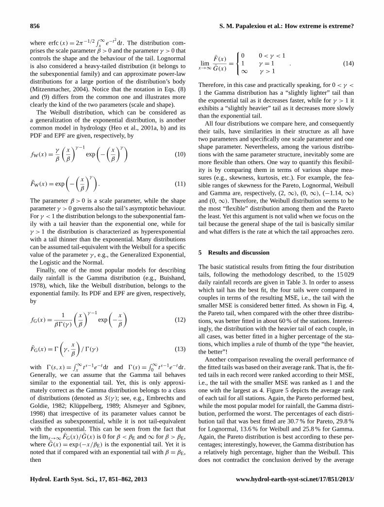
We searched for the existence of any geographical pat-terns, potentially defining climatic zones, in the best fittedtails, i.e., the existence of zones in the world where the ma-jority of the records were better described by one of the stud-ied distribution tails. The maps in Fig. 7, which depict thelocations of the stations where each distribution tail was bestfitted, did not unveil any regular patterns in terms of the bestfitted distribution but rather seem to follow a random varia-tion.

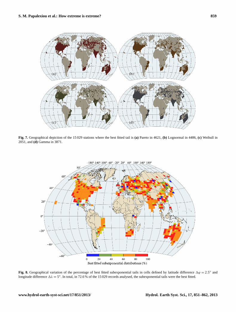
Another way to investigate for geographical patterns, asthe previous map did not reveal any useful information, isto study the fitted tails grouped into two coarser groups: thesubexponential group and the exponential-hyperexponentialgroup. The former includes the Pareto, the Lognormal andthe Weibull with γ < 1 tails, while the latter includes theGamma and the Weibull withγ ≥ 1 tails. Among the 15 029records, subexponential tails were best fitted in 10 911 casesor in 72.6 % while exponential-hyperexponential tails werebest fitted in 4 118 or in 27.4 %. Further, in order to get aclearer picture instead of constructing maps with the loca-tions where the first-group or the second-group tails werebest fitted, we studied the percentage of subexponential tailsthat were best fitted in large regions. Specifically, we con-structed a grid covering the entire earth using a latitudedifference1ϕ = 2.5◦ and longitude difference1λ = 5◦. Ineach grid cell we estimated the percentage of the best fittedsubexponential tails simply by counting the number of thebest fitted subexponential tails divided by the total numberof records within the cell. We present these percentages inthe form of a map in Fig. 8, using a colour scale as shownin the map’s legend. The cells plotted in the map are thosecontaining at least two records, so that the calculation of per-centages have some meaning.

www.hydrol-earth-syst-sci.net/17/851/2013/ Hydrol. Earth Syst. Sci., 17, 851–862, 2013

858 S. M. Papalexiou et al.: How extreme is extreme?

Fig. 5. Mean ranks of the tails for all records. The best-fitted tailis ranked as 1 while the worst-fitted as 4. A lower average rankindicates a better performance.

The map of Fig. 8 clearly shows that in the vast majorityof cells subexponential tails dominate (percentage> 60 %).Particularly, out of 532 cells having at least two records, 255and 163 have percentages of subexponential tails 60–80 %and> 80 %, respectively. In contrast, in only 35 and 79 cellsare the percentage values in the ranges 0–40 % and 40–60 %,respectively.

6 Verification of the fitting method

The use of a different norm for fitting the tail into the em-pirical data could potentially modify the conclusions drawn.Nevertheless, this argument is pointless in the sense that themain concern should be the efficiency of the norm used, i.e.,if it possesses desired properties, e.g., if it is unbiased and haslower variance in comparison to other candidates. Usually,the error is expressed in terms of random variable values,e.g., rainfall values, and not in terms of probability. However,a literature search did not reveal or verify that the commonlyused norms, e.g., the classical MSE norm, are better than thenorm N1 used here (see Eq. 5).

For this reason, we implemented a Monte Carlo scheme,which actually replicates the method we followed, where weevaluate the performance of the norm N1 and also compareit with the more common norms N2 and N3 defined as

N2 =1

N

n∑i=n−N+1

(xu

x(i)

− 1

)2

(15)

N3 =1

N

n∑i=n−N+1

(xu − x(i)

)2. (16)

Here,xu = Q(u) is the value predicted by the quantile func-tion Q of the distribution under study foru equal to the em-pirical probability ofx(i) (the ith element the sample ranked

Fig. 6.Histograms of the shape parameters of the fitted tails.

in ascending order) according to the Weibull plotting posi-tion. The norm N2 has the same rationale as the one we usedbut the error is estimated in terms of rainfall values, ratherthan in terms of probability, while the norm N3 is the classi-cal and most commonly used MSE norm.

The Monte Carlo scheme we performed can be summa-rized in the following steps: (a) we generated 1000 randomsamples from each one of the four distributions we studiedwith sample size equal to 6600 values, which is approxi-mately the average number of nonzero daily rainfall valuesper record; (b) we selected the scale and the shape parametervalues to be approximately equal with the median values re-sulted from the analysis of the real world dataset (see Table 3)in order for the generated random samples to be representa-tive of the real data; and (c) we fitted each distribution toits corresponding random sample and estimated the parame-ters by applying our method for each one of the three norms,while we setN equal to 80 yr, which is approximately theaverage record length.

The results are presented in Fig. 9. The whiskers of thebox plots express the 95 % Monte Carlo confidence intervalof the parameters while the dashed lines show the true param-eter values. It is clear that the norm N1 we used results in al-most unbiased estimation of the parameters while, especiallyfor the Pareto and the Lognormal distributions, it results inmarkedly smaller variance compared to the classical normN3. The norm N2 seems to perform very well for the Pareto,Lognormal and Weibull distributions (although somewhat bi-ased) but the results are poor for the Gamma distribution.The classical and the most commonly used norm N3 is by farthe worst in term of bias except for the Gamma distribution,for which it performs equally well as N1. In particular, forthe subexponential distributions of this simulation, i.e., thePareto, the Lognormal and the Weibull, the classical normN3 fails to provide good results. This may point to a moregeneral conclusion, i.e., that the classical MSE, which is in-spired based on properties of the normal distribution, is not

Hydrol. Earth Syst. Sci., 17, 851–862, 2013 www.hydrol-earth-syst-sci.net/17/851/2013/

S. M. Papalexiou et al.: How extreme is extreme? 859

Fig. 7. Geographical depiction of the 15 029 stations where the best fitted tail is(a) Pareto in 4621,(b) Lognormal in 4486,(c) Weibull in2051, and(d) Gamma in 3871.

Fig. 8. Geographical variation of the percentage of best fitted subexponential tails in cells defined by latitude difference1ϕ = 2.5◦ andlongitude difference1λ = 5◦. In total, in 72.6 % of the 15 029 records analysed, the subexponential tails were the best fitted.

www.hydrol-earth-syst-sci.net/17/851/2013/ Hydrol. Earth Syst. Sci., 17, 851–862, 2013

860 S. M. Papalexiou et al.: How extreme is extreme?

Fig. 9. Results of a Monte Carlo scheme implemented to evaluatethe performance of the norm N1 used in fitting of tails in this study,in comparison to commonly used ones (N2, N3).

a good choice for subexponential distributions. This needs tobe further investigated; however, we deem that there is a ra-tionale supporting the following conclusion: subexponentialdistributions can generate “extremely” extreme values com-pared to the main “body” of values, and thus, in the classicalnorm these values will contribute “extremely” to the total er-ror heavily affecting the fitting results.

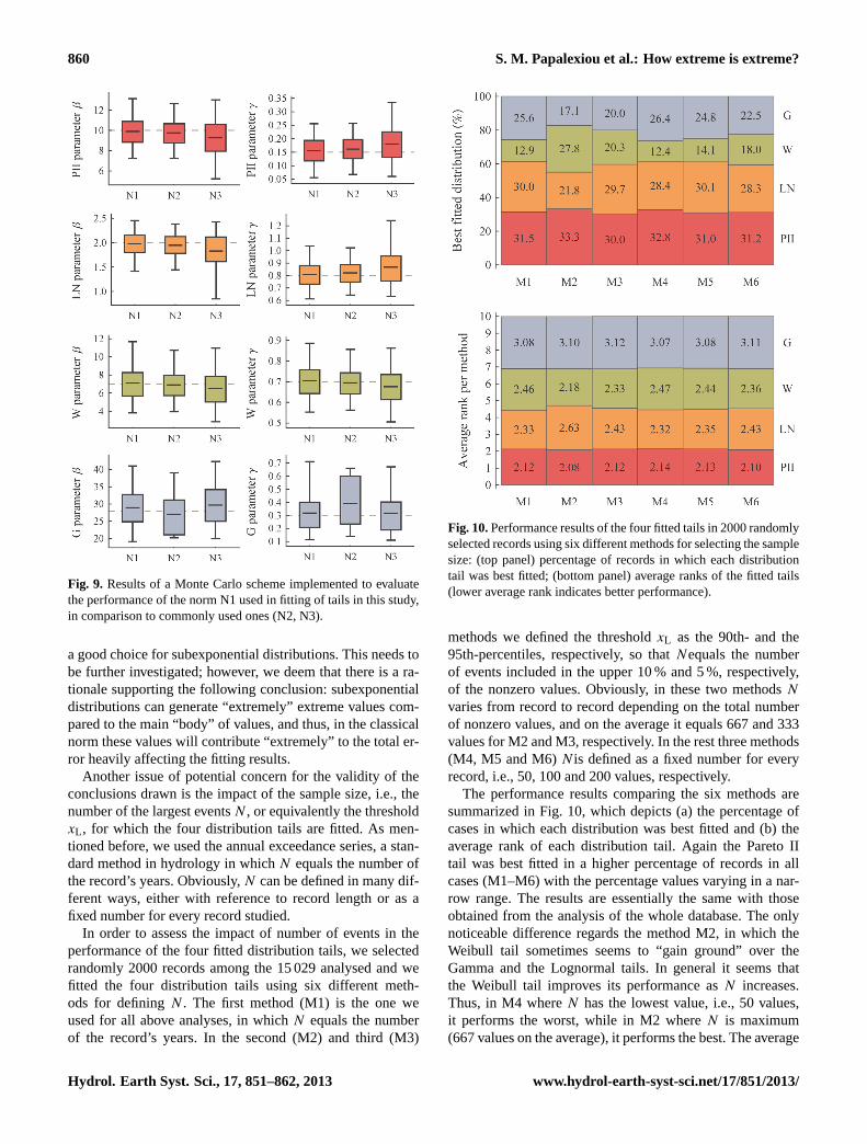
Another issue of potential concern for the validity of theconclusions drawn is the impact of the sample size, i.e., thenumber of the largest eventsN , or equivalently the thresholdxL , for which the four distribution tails are fitted. As men-tioned before, we used the annual exceedance series, a stan-dard method in hydrology in whichN equals the number ofthe record’s years. Obviously,N can be defined in many dif-ferent ways, either with reference to record length or as afixed number for every record studied.

In order to assess the impact of number of events in theperformance of the four fitted distribution tails, we selectedrandomly 2000 records among the 15 029 analysed and wefitted the four distribution tails using six different meth-ods for definingN . The first method (M1) is the one weused for all above analyses, in whichN equals the numberof the record’s years. In the second (M2) and third (M3)

Fig. 10.Performance results of the four fitted tails in 2000 randomlyselected records using six different methods for selecting the samplesize: (top panel) percentage of records in which each distributiontail was best fitted; (bottom panel) average ranks of the fitted tails(lower average rank indicates better performance).

methods we defined the thresholdxL as the 90th- and the95th-percentiles, respectively, so thatNequals the numberof events included in the upper 10 % and 5 %, respectively,of the nonzero values. Obviously, in these two methodsN

varies from record to record depending on the total numberof nonzero values, and on the average it equals 667 and 333values for M2 and M3, respectively. In the rest three methods(M4, M5 and M6)N is defined as a fixed number for everyrecord, i.e., 50, 100 and 200 values, respectively.

The performance results comparing the six methods aresummarized in Fig. 10, which depicts (a) the percentage ofcases in which each distribution was best fitted and (b) theaverage rank of each distribution tail. Again the Pareto IItail was best fitted in a higher percentage of records in allcases (M1–M6) with the percentage values varying in a nar-row range. The results are essentially the same with thoseobtained from the analysis of the whole database. The onlynoticeable difference regards the method M2, in which theWeibull tail sometimes seems to “gain ground” over theGamma and the Lognormal tails. In general it seems thatthe Weibull tail improves its performance asN increases.Thus, in M4 whereN has the lowest value, i.e., 50 values,it performs the worst, while in M2 whereN is maximum(667 values on the average), it performs the best. The average

Hydrol. Earth Syst. Sci., 17, 851–862, 2013 www.hydrol-earth-syst-sci.net/17/851/2013/

S. M. Papalexiou et al.: How extreme is extreme? 861

rank, which is a better measure of the overall performance ofthe distribution tails, remains essentially the same for eachdistribution in all methods. An exception is observed againin M2 where the Weibull tail performs better than the Log-normal tail. Apart from this exception the general conclusionis again that the Pareto II performs the best, followed by theLognormal and the Weibull tails, while the Gamma tail per-forms the worst in all cases.

7 Summary and conclusions

Daily rainfall records from 15 029 stations are used to inves-tigate the performance of four common tails that correspondto the Pareto, the Weibull, the Lognormal and the Gammadistributions. These theoretical tails were fitted to the empir-ical tails of the records and their ability to adequately capturethe behaviour of extreme events was quantified by comparingthe resulting MSE. The ranking from best to worst in termsof their performance is (a) the Pareto, (b) the Lognormal,(c) the Weibull, and (d) the Gamma distributions. The anal-ysis suggests that heavier-tailed distributions in general per-formed better than their lighter-tailed counterparts. Particu-larly, in 72.6 % of the records subexponential tails were betterfitted while the exponential-hyperexponential tails were bet-ter fitted is only 27.4 %. It is instructive that the most popularmodel used in practice, the Gamma distribution, performedthe worst, revealing that the use of this distribution under-estimates in general the frequency and the magnitude of ex-treme events. Nevertheless, we must not neglect the fact thatthe Gamma distribution was the best fitted in 25.8 % of therecords.

Additionally, we note that heavy tails tend to be hidden(see, e.g., Koutsoyiannis, 2004a, b; Papalexiou and Kout-soyiannis, 2013), especially when the sample size is small.Thus, we believe that even in the cases where the Gamma tailperformed well, the true underlying distribution tail may beheavier. This leads to the recommendation that heavy-taileddistributions are preferable as a means to model extreme rain-fall events worldwide. We also note that the tails studiedhere are as simple as possible, i.e., only one shape parame-ter controls their asymptotic behaviour. Yet there are manydistributions with more than one shape parameters whichmay affect their tail behaviour. Particularly, the GeneralizedGamma (Stacy, 1962) and the Burr type XII distributionswere compared as candidates for the daily rainfall (based onL-moments) in anonther study, using thousands of empiricaldaily records and the former performed better (Papalexiouand Koutsoyiannis, 2012).

The key implication of this analysis is that the frequencyand the magnitude of extreme events have generally been un-derestimated in the past. Engineering practice needs to ac-knowledge that extreme events are not as rare as previouslythought and to shift toward more heavy-tailed probability dis-tributions.

Acknowledgements.Four eponymous reviewers, Aaron Clauset,Roberto Deidda, Salvatore Grimaldi and Francesco Laio, and fourcommenters, Santiago Beguerıa, Federico Lombardo, Chris Onofand Patrick Willems, are acknowledged for their public reviewcomments, as is the editor Peter Molnar for his personal comments.Most of the comments helped us to improve the original manuscript.

Edited by: P. Molnar

References

Ahmad, M. I., Sinclair, C. D., and Werritty, A.: Log-logistic floodfrequency analysis, J. Hydrol., 98, 205–224,doi:10.1016/0022-1694(88)90015-7, 1988.

Alsmeyer, G. and Sgibnev, M.: On the tail behaviour of the supre-mum of a random walk defined on a Markov chain, available at:http://kamome.lib.ynu.ac.jp/dspace/handle/10131/5689(last ac-cess: 10 November 2012), 1998.

Balkema, A. A. and De Haan, L.: Residual Life Time at Great Age,Ann. Probab., 2, 792–804,doi:10.1214/aop/1176996548, 1974.

Beguerıa, S., Vicente-Serrano, S. M., Lopez-Moreno, J. I., andGarcıa-Ruiz, J. M.: Annual and seasonal mapping of peak in-tensity, magnitude and duration of extreme precipitation eventsacross a climatic gradient, northeast Spain, Int. J. Climatol., 29,1759–1779, 2009.

Ben-Zvi, A.: Rainfall intensity–duration–frequency relationshipsderived from large partial duration series, J. Hydrol., 367, 104–114,doi:10.1016/j.jhydrol.2009.01.007, 2009.

Bhattarai, K. P.: Partial L-moments for the analysis of censoredflood samples, Hydrolog. Sci. J., 49, 855–868, 2004.

Buishand, T. A.: Some remarks on the use of daily rainfall mod-els, J. Hydrol., 36, 295–308,doi:10.1016/0022-1694(78)90150-6, 1978.

Burr, I. W.: Cumulative Frequency Functions, Ann. Math. Stat., 13,215–232, 1942.

Chow, V. T.: Handbook of applied hydrology: a compendium ofwater-resources technology, McGraw-Hill, 1964.

Cunnane, C.: A particular comparison of annual maxima and partialduration series methods of flood frequency prediction, J. Hydrol.,18, 257–271,doi:10.1016/0022-1694(73)90051-6, 1973.

El Adlouni, S., Bobee, B., and Ouarda, T. B. M. J.: On the tails ofextreme event distributions in hydrology, J. Hydrol., 355, 16–33,doi:10.1016/j.jhydrol.2008.02.011, 2008.

Embrechts, P. and Goldie, C. M.: On convolution tails, Stoch. Proc.Appl., 13, 263–278,doi:10.1016/0304-4149(82)90013-8, 1982.

Embrechts, P., Kluppelberg, C., and Mikosch, T.: Modelling ex-tremal events for insurance and finance, Springer Verlag, BerlinHeidelberg, 1997.

European Commission: Directive 2007/60/EC of the European Par-liament and of the Council of 23 October 2007 on the assessmentand management of flood risks, Official Journal of the EuropeanCommunities, L, 288(6.11), 27–34, 2007.

Goldie, C. M. and Kluppelberg, C.: Subexponential distributions,in: A Practical Guide to Heavy Tails: Statistical Techniques andApplications, edited by: Adler, R., Feldman, R., and Taggu, M.S., 435–459, Birkhauser Boston, 1998.

Gupta, S. K.: Modern Hydrology and Sustainable Water Develop-ment, John Wiley & Sons, 2011.

www.hydrol-earth-syst-sci.net/17/851/2013/ Hydrol. Earth Syst. Sci., 17, 851–862, 2013

862 S. M. Papalexiou et al.: How extreme is extreme?

Heo, J. H., Boes, D. C., and Salas, J. D.: Regional flood fre-quency analysis based on a Weibull model: Part 1. Estimationand asymptotic variances, J. Hydrol., 242, 157–170, 2001a.

Heo, J. H., Salas, J. D., and Boes, D. C.: Regional flood frequencyanalysis based on a Weibull model: Part 2. Simulations and ap-plications, J. Hydrol., 242, 171–182, 2001b.

Hershfield, D. M.: Estimating the probable maximum precipitation,J. Hydraul. Eng.-ASCE, 87, 99–106, 1961.

Kl uppelberg, C.: Subexponential Distributions and Integrated Tails,J. Appl. Probab., 25, 132–141,doi:10.2307/3214240, 1988.

Kl uppelberg, C.: Subexponential distributions and characteriza-tions of related classes, Probab. Theory Rel., 82, 259–269,doi:10.1007/BF00354763, 1989.

Koutsoyiannis, D.: A probabilistic view of Hershfield’s method forestimating probable maximum precipitation, Water Resour. Res.,35, 1313–1322, 1999.

Koutsoyiannis, D.: Statistics of extremes and estimation of extremerainfall, 1, Theoretical investigation, Hydrolog. Sci. J., 49, 575–590, 2004a.

Koutsoyiannis, D.: Statistics of extremes and estimation of extremerainfall, 2, Empirical investigation of long rainfall records, Hy-drolog. Sci. J., 49, 591–610, 2004b.

Kroll, C. N. and Stedinger, J. R.: Estimation of moments and quan-tiles using censored data, Water Resour. Res., 32, 1005–1012,1996.

Mielke Jr., P. W.: Another Family of Distributions for Describingand Analyzing Precipitation Data, J. Appl. Meteorol., 12, 275–280, 1973.

Mielke Jr., P. W. and Johnson, E. S.: Some generalized beta distri-butions of the second kind having desirable application featuresin hydrology and meteorology, Water Resour. Res., 10, 223–226,1974.

Mitzenmacher, M.: A brief history of generative models for powerlaw and lognormal distributions, Internet Mathematics, 1, 226–251, 2004.

Moisello, U.: On the use of partial probability weighted momentsin the analysis of hydrological extremes, Hydrol. Process., 21,1265–1279, 2007.

Papalexiou, S. M. and Koutsoyiannis, D.: Entropy based derivationof probability distributions: A case study to daily rainfall, Adv.Water Resour., 45, 51–57,doi:10.1016/j.advwatres.2011.11.007,2012.

Papalexiou, S. M. and Koutsoyiannis, D.: Battle of extreme valuedistributions: A global survey on extreme daily rainfall, WaterResour. Res., online first,doi:10.1029/2012WR012557, 2013.

Pickands III, J.: Statistical Inference Using Extreme Order Statis-tics, Ann. Stat., 3, 119–131, 1975.

Stacy, E. W.: A Generalization of the Gamma Distribution, Ann.Math. Stat., 33, 1187–1192, 1962.

Tadikamalla, P. R.: A Look at the Burr and Related Distributions,Int. Stat. Rev., 48, 337–344, 1980.

Tavares, L. V. and Da Silva, J. E.: Partial duration series method re-visited, J. Hydrol., 64, 1–14,doi:10.1016/0022-1694(83)90056-2, 1983.

Teugels, J.: Class of subexponential distributions, Ann. Probab., 3,1000–1011,doi:10.1214/aop/1176996225, 1975.

Wang, Q. J.: Using partial probability weighted moments to fit theextreme value distributions to censored samples, Water Resour.Res., 32, 1767–1771, 1996.

Werner, T. and Upper, C.: Time variation in the tail behavior ofBund future returns, J. Future Markets, 24, 387–398, 2004.

Hydrol. Earth Syst. Sci., 17, 851–862, 2013 www.hydrol-earth-syst-sci.net/17/851/2013/