portfolio optimization with trend following strategies

Portfolio optimization with trend followingstrategies- A comparative study of methods for portfolio optimization appliedon trend following trading strategies in the futures market.Master’s thesis in Engineering Mathematics and Computational Science

Samuel Rubenson

Department of MathematicsChalmers University of TechnologyGothenburg, Sweden 2016

Abstract

This thesis investigates how the mean-variance framework for portfolio optimizationcompare against that of risk-parity and the minimum-CVaR portfolio. Within therisk measure of portfolio variance, we find that the performance of the mean-varianceportfolio is highly dependent on a well-conditioned sample covariance matrix whilerisk-parity appears to offer increased numerical stability. But with a regularizedestimate, no method consistently outperform the other. We suggest a minor exten-sion to the risk-parity allocation objective with a resulting portfolio that exhibitssuperior properties in several central aspects. The minimum-CVaR portfolio is builtaround the alternative risk measure conditional value at risk and we find that whilethe original problem formulation is prone to overfitting, a regularized version showspromising results worthy of further investigation.

Acknowledgements

I want to express my gratitude to Lynx Asset Management for making it possiblefor me to carry out this thesis work and for offering me a friendly work environment.Special thanks go to Tobias Rydén, the main supervisor of this thesis, for his guid-ance and advise throughout the whole process. I also want to thank Ola Backmanfor many valuable discussions on the direction of this thesis.

Finally I want to thank Patrik Albin, my supervisor and examiner at Chalmers, forhis help administrating and completing this thesis.

Samuel Rubenson, Stockholm, January 2017

iii

Contents

1 Introduction 11.1 Futures contracts . . . . . . . . . . . . . . . . . . . . . . . . . . . . . 11.2 Background . . . . . . . . . . . . . . . . . . . . . . . . . . . . . . . . 21.3 Thesis outline . . . . . . . . . . . . . . . . . . . . . . . . . . . . . . . 2

2 Data and parameters 32.1 Price data and returns . . . . . . . . . . . . . . . . . . . . . . . . . . 32.2 Dependence structure . . . . . . . . . . . . . . . . . . . . . . . . . . . 4

2.2.1 Regularized correlation estimate . . . . . . . . . . . . . . . . . 52.3 Prediction model . . . . . . . . . . . . . . . . . . . . . . . . . . . . . 6

3 Models 93.1 Mean-Variance portfolio . . . . . . . . . . . . . . . . . . . . . . . . . 93.2 Risk-Parity portfolio . . . . . . . . . . . . . . . . . . . . . . . . . . . 11

3.2.1 Extension to negative weights . . . . . . . . . . . . . . . . . . 123.2.2 Modified risk-parity . . . . . . . . . . . . . . . . . . . . . . . . 133.2.3 Lagrangian relaxation of the RP problem . . . . . . . . . . . . 133.2.4 Solving the RP optimization problem in practice . . . . . . . . 14

3.2.4.1 The x-update . . . . . . . . . . . . . . . . . . . . . . 153.2.4.2 The z-update . . . . . . . . . . . . . . . . . . . . . . 15

3.2.5 Exploring different RP portfolios . . . . . . . . . . . . . . . . 163.3 Minimum conditional value-at-risk portfolio . . . . . . . . . . . . . . 17

3.3.1 Extensions . . . . . . . . . . . . . . . . . . . . . . . . . . . . . 183.3.1.1 Using a fixed α . . . . . . . . . . . . . . . . . . . . . 183.3.1.2 Regularization . . . . . . . . . . . . . . . . . . . . . 193.3.1.3 Piecewise linear penalty . . . . . . . . . . . . . . . . 203.3.1.4 Efficient solver . . . . . . . . . . . . . . . . . . . . . 20

4 Methods 254.1 Choice of filter parameters . . . . . . . . . . . . . . . . . . . . . . . . 25

4.1.1 Variance estimate . . . . . . . . . . . . . . . . . . . . . . . . . 254.1.2 Correlation estimate . . . . . . . . . . . . . . . . . . . . . . . 25

4.2 Model evaluation . . . . . . . . . . . . . . . . . . . . . . . . . . . . . 25

5 Results 295.1 Comparing MV and RP . . . . . . . . . . . . . . . . . . . . . . . . . 29

v

Contents

5.1.1 Factors that have an impact on results . . . . . . . . . . . . . 305.2 LES . . . . . . . . . . . . . . . . . . . . . . . . . . . . . . . . . . . . 375.3 Results for different prediction models . . . . . . . . . . . . . . . . . 42

6 Discussion 45

Bibliography 47

vi

1Introduction

This thesis is written in cooperation with Lynx Asset Management, a hedge fundthat trades on futures markets for equities, commodities, currencies and bonds. Suchfunds are often referred to as Commodity trading advisors, or a CTA funds. Lynx’sinvestment strategies are solely based on quantitative models, and the process ofdeciding which positions to take in different assets can naturally be divided into twosteps. The first step is prediction, where based on historical data a prediction modelgenerates a signal indicating a direction (usually combined with a signal strength)that prices in different assets are expected to follow. The second step, the portfoliostep, aims at combining the available assets in a way that yields a favorable risk/re-turn profile based on the signals generated by the prediction model together withsome measure of risk. This thesis will focus on the second step, i.e. methods forportfolio optimization, applied to trend following trading strategies.

1.1 Futures contracts

A futures contract is a type of financial derivative, meaning that its current valueor future payoff is a function of the price of some underlying asset, for example astock market index. Specifically it is a standardized forward contract. A forwardcontract between two parties stipulates that one party must buy and the other onesell, a specific underlying asset for an agreed upon price at a specified future time.Forward contracts are well suited to hedge risk exposure to commodities, currenciesetc., in a way that provides physical delivery of the underlying asset at the timeof maturity. For example, say that a non-American company receives an order todeliver a product in one year and will be paid $100 at that time. The value of $1in the native currency will most likely be different at the time of payment, hencethe company has a risk exposure to the exchange rate between the two currencies.To hedge this risk, the company may enter a forward contract such that it one yearfrom now will receive a specified amount in the native currency in exchange for $100,thus removing the risk of the US dollar losing value compared to the native currency.

The exchange traded futures contract is better suited for pure speculation in theprice of the underlying asset. Similar to a forward contract there is no cost associatedwith entering a futures contract. But to reduce the risk of default, there is a dailycash settlement corresponding to the price change of the futures contract over thatday. This cash settlement is transferred between the two parties’ margin accounts

1

1. Introduction

associated with the open position. The size of the margin account generally dependon the value of the underlying asset and the volatility of its price.

1.2 BackgroundClassic portfolio theory mainly deals with the problem of allocating capital. Thatis, the problem of investing a fixed capital in different available assets, typically bybuying stocks and bonds. For a CTA fund the problem becomes a bit different seeingas when trading futures, only a fraction of the position value is required for a marginaccount and the win/loss of a position is settled daily. Basically no capital is neededto take on positions, thus the interest does not lie in the allocation of capital butrather in finding an interrelation between positions in different assets (the portfolio)that has desired properties based on current information. The absolute position sizeswill only scale the realized win/loss and is thus based on how much risk is desired toundertake. Further, when trading on futures markets there is no practical differencebetween attaining a long or a short position in an asset, making it easier to constructa well hedged portfolio that has low correlation with the ”market portfolio”.

1.3 Thesis outlineThe purpose of this thesis is to compare and improve three existing methods for port-folio optimization, with the main aim of investigating if alternatives to the standardMarkowitz model could show superior portfolio properties. The second chapter willpresent the input to these models in the form of data and parameters. Chapter 3 willreview three different methods for portfolio selection, their original form along withsuggested extensions. Both the theoretical aspects of the optimization problems aswell as efficient ways of solving them in practice will be covered in this chapter.Chapters 4 and 5 covers the methods for evaluation together with the results andincludes an investigation of how the models compare under different circumstances,how sensitive their performance is to changes in the input parameters and finallyhow the relative performance is dependent on the underlying trading model.

2

2Data and parameters

2.1 Price data and returns

The data set considered throughout this thesis contains daily observations of theOpen, Close, High and Low futures price of 74 different underlying assets datingback as far as 1980. The collection of assets are a wide mix of stock market indices,commodities, currencies and bonds. As discussed in section 1.1, a futures contracthas a limited time to maturity after which the derivative ceases to exist. Thus con-structing a continuous time series containing the futures price for an asset involvespatching together price series for similar contracts over time. Although there willgenerally be jumps in a raw combination of such time series, these jumps can be re-moved in a way that preserves the daily futures price differences (but not the actualprice) which is convenient when analysis is based on returns.

Let {St}Tt=0 be the price series of an asset over time. To simplify analysis whenworking with time series, a common practice is to transform the data in such a waythat it can be assumed to be a stationary process, implying a time independentmean and variance. In general a financial price series St can not be assumed to havea constant mean, but for the return series dSt defined as

dSt = St − St−1,

a close to zero mean can generally be assumed. Many empirical studies does howevershow that financial return series have a time dependent variance, often referred to asvolatility clustering [3]. To remove this property and make time series for differentassets comparable the return series will be normalized as

dSt = dStσt−1

, (2.1)

where σt is the standard deviation of the time series S at time t. Using σt−1 inequation (2.1) keeps dS a martingale process. Note that with this normalizationreturns are additive both over time and over assets where the unit now is standarddeviations. To obtain the normalized returns requires an estimate of the standarddeviation at each time step t. There are several ways to obtain such an estimatebut a popular method making use of both the Open, Close, High and Low price wasproposed by D.Yang and Q.Zhang [11].

3

2. Data and parameters

Let Ot, Ht, Lt, Ct be the time series containing open, high, low and close prices ofan asset. The rolling variance estimate σ2

t for this asset will be estimated accordingto Yt = (Ot − Ct−1)2 + 1

2(Ht − Lt)2 − (2 log 2− 1)(Ot − Ct)2

σ2t = ασ2

t−1 + (1− α)Yt,(2.2)

where α ∈ [0, 1] is a filter parameter that determines how fast ”old” data shouldbe forgotten. Letting α = 1− 1

τ, the parameter τ can loosely be interpreted as the

mean of how far back in time the filter weights are placed.

The transformed time series of normalized returns is denoted by

dZt = dStσt−1

,

and is assumed to have constant zero mean and unit variance. This time series dZtwill be referred to as normalized returns and is considered in all analysis throughoutthis thesis.

2.2 Dependence structureIn order to construct a portfolio with a desiered risk profile some measure of riskneeds to be defined. A very common measure is the standard deviation, or volatility,of portfolio returns.

Let our universe consist ofM assets for which the normalized returns can be modeledas random variables with zero mean and unit variance. Further, let w ∈ RM be theposition vector defining a portfolio P . Each position wi has the unit of standarddeviations and thus |wi| describes how much risk is taken in asset i; the sign ofwi represents a long (positive) or a short (negative) position. The variance of theportfolio returns RP can then be defined as

Var(RP ) =M∑i=1

M∑i=1

wiwjσi,j,

where σi,j is the correlation coefficient between assets i and j. In matrix notationthis is written as

Var(RP ) = wTΣw,

where Σ ∈ RM×M is the correlation matrix and (.)T denotes the transpose of a vector.

While the considered time series for each asset is assumed to be stationary with atime invariant variance, this is not assumed for correlations between assets. Thusfor all t ∈ {1, . . . , T} we seek to estimate

Σt = E[dZtdZTt ] ∈ RM×M ,

4


where we now consider the vector form of returns, i.e. dZt ∈ RM . Using only thesecond moment assumes that the squared expected values of returns are if non zeromuch smaller than the expected squared value, that is

E[dZt,idZt,j]� E[dZt,i]E[dZt,j] ∀i, j.

The correlation matrix Σt at time t will be taken as a linear combination of dailyobservations according to

Σt =t−1∑s=0

csdZt−sdZTt−s,

where cs are filter coefficients. Again there is a wide variety of options in how toset this coefficient but focus will be kept on variations of an exponential movingaverage, i.e. a coefficient with exponential decay.

In practice problems can arise from the fact that the estimates for assets at thebeginning of their time series can be unstable and to deal with this a burn-in periodis introduced, meaning that we enforce that X number of historical data points arerequired in order to use the correlation estimate. The main reason for this (besidesa stable estimate) is to ensure that the estimated matrix will be positive definitewhich numerically may not hold for daily observations. This is a crucial property ofa correlation matrix ensuring a strictly positive variance of portfolio returns.An exponential moving average of the daily observations can be written as

Σt =t−1∑s=0

(1− α)αsdZt−sdZTt−s,

with α ∈ [0, 1]. Now the half-life s of a daily observation can be solved for by

(1− α)αs = (1− α)2 ⇒ s = − log 2

logα.

Letting α = 1 − 1τ, s ≈ τ log 2. The parameter τ is used as input when estimating

Σt; some multiple of the half-life τ log 2 could be a reasonable way to set the burn-inperiod.

2.2.1 Regularized correlation estimateEstimating a high-dimensional correlation matrix quickly becomes a difficult prob-lem. In a setting with M assets, there are (M2 −M)/2 parameters to estimate. Inour case of M = 74 that is 2701 parameters and it is safe to assume that there willbe large errors in many of these estimates.

A frequently observed property of the sample correlation matrix is a high conditionnumber [4], i.e. that the matrix is ill-conditioned and it is not uncommon to see closeto singular estimates. In many applications making use of the correlation matrix,this property may amplify errors. An example is when solving a linear system

5


of equations where the solution involves the precision matrix (inverse correlationmatrix).As we will see later, this problem applies to some methods for portfolio optimiza-tion, and a common approach to increase numerical stability is regularization of thesample correlation matrix.

Recall that for a normal matrix A, the condition number κA can be calculated as

κA = |λmax(A)||λmin(A)| ,

where λ refers to eigenvalues. It has been suggested in [7] that the larger eigenvaluesof the correlation matrix are generally overestimated whilst the smaller eigenvaluesare underestimated. To overcome the problem of an ill-conditioned matrix andreduce the impact of estimation errors, Ledoit and Wolf proposed a shrinkage esti-mator for the correlation matrix, a linear combination of Σ and the identity matrixI [4]. Consider adding some factor of the identity matrix to Σ according to

Σ = Σ + λI, (2.3)

where λ ∈ R. As the correlation matrix is symmetric, it can be decomposed as

Σ = PDP T

where P is a orthogonal matrix consisting of eigenvectors of Σ, and D is a diagonalmatrix with the corresponding eigenvalues. It is easy to see that

PDP T + λI = P (D + λI)P T ,

and thus adding some multiple of the identity matrix to Σ will increase all eigenvaluesby the constant λ. Note that the eigenvalues ordering by size stays unchanged.This approach deals with the potential problems of a close to singular estimate,a high condition number, and the confidence placed on directions with very largeor small eigenvalues. Note in equation (2.3) that as λ increases towards infinitythe properties of the regularized correlation matrix approaches that of the identitymatrix. To simplify evaluation, the shrinkage estimator will be calculated as

Σ = (1− λ)Σ + λI,

where λ ∈ [0, 1] will be referred to as the regularization coefficient or the degree ofregularization.

2.3 Prediction modelWhen constructing a portfolio we want to take into account our beliefs about fu-ture price movements generated from some prediction model (or trading strategy).CTA funds generally use a variety of trading strategies to meet their investment

6


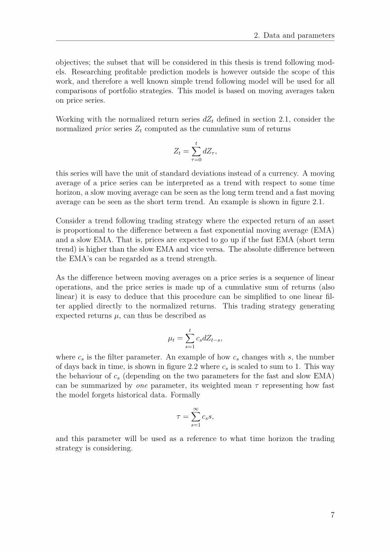
objectives; the subset that will be considered in this thesis is trend following mod-els. Researching profitable prediction models is however outside the scope of thiswork, and therefore a well known simple trend following model will be used for allcomparisons of portfolio strategies. This model is based on moving averages takenon price series.

Working with the normalized return series dZt defined in section 2.1, consider thenormalized price series Zt computed as the cumulative sum of returns

Zt =t∑

τ=0dZτ ,

this series will have the unit of standard deviations instead of a currency. A movingaverage of a price series can be interpreted as a trend with respect to some timehorizon, a slow moving average can be seen as the long term trend and a fast movingaverage can be seen as the short term trend. An example is shown in figure 2.1.

Consider a trend following trading strategy where the expected return of an assetis proportional to the difference between a fast exponential moving average (EMA)and a slow EMA. That is, prices are expected to go up if the fast EMA (short termtrend) is higher than the slow EMA and vice versa. The absolute difference betweenthe EMA’s can be regarded as a trend strength.

As the difference between moving averages on a price series is a sequence of linearoperations, and the price series is made up of a cumulative sum of returns (alsolinear) it is easy to deduce that this procedure can be simplified to one linear fil-ter applied directly to the normalized returns. This trading strategy generatingexpected returns µ, can thus be described as

µt =t∑

s=1csdZt−s,

where cs is the filter parameter. An example of how cs changes with s, the numberof days back in time, is shown in figure 2.2 where cs is scaled to sum to 1. This waythe behaviour of cs (depending on the two parameters for the fast and slow EMA)can be summarized by one parameter, its weighted mean τ representing how fastthe model forgets historical data. Formally

τ =∞∑s=1

css,

and this parameter will be used as a reference to what time horizon the tradingstrategy is considering.

7


PriceSlow EMAFast EMA

Figure 2.1: An example of a long and a short moving average taken on a priceseries.

0 50 100 150 200 250 300 350 400 450 5000

1

2

3

4

5

6

7 ·10−3

s

c s

τ = 125

Figure 2.2: The coefficient value cs placed on returns s time steps back in ourconsidered trend following trading strategy, here with ”mean” τ = 125.

8

3Models

3.1 Mean-Variance portfolio

The foundation of modern portfolio theory was laid out by Harry Markowitz in hispaper on Portfolio Selection in 1952 [6]. He proposed a model for constructing anoptimal portfolio, where optimal is under the assumption that investors are rationaland seek high returns with low risk.

Let y ∈ RM be a random variable representing the normalized returns (from section2.1) of the M markets in our universe. Further, let y have an arbitrary distributionbut assume that its first and second moments are well defined and finite. That is

−∞ < E[yi] <∞ ∀i,E[y2

i ] <∞ ∀i.

Consider constructing a portfolio consisting of these M assets, and let w ∈ RM

denote the positions vector. Then the random variable yp = yTw is the portfolioreturn and its first two moments are computed as

E[yp] =M∑i=1

wiE[yi] = µTw,

E[y2p] =

M∑i=1

M∑i=1

wiwjE[yiyj] = wTΣw, (3.1)

where µ and Σ denote the expected returns and the correlation matrix respectively.In mean-variance (MV) analysis, only the first two moments are considered and therisk of a portfolio is quantified by the variance of returns which will be approximatedby equation (3.1). The objective is to find an optimal trade-off between risk andreturn, in the sense that the portfolio weights w maximize the expected return fora given portfolio variance (propensity for risk), i.e. w solves the problem

maxw

µTw

s.t. wTΣw ≤ σ2TGT .

(3.2)

With a linear objective function maximized over a convex set (Σ is positive definite),this problem is clearly convex. For σ2

TGT > 0, the Karush-Kuhn-Tucker (KKT)

9

3. Models

conditions are both necessary and sufficient to ensure global optimality [1, p. 142-143]. The KKT conditions for (3.2) become

µ+ νΣw = 0M , (3.3)ν(wTΣw − σ2

TGT ) = 0, (3.4)ν ≥ 0,

where ν is the Lagrange multiplier. Now, equation (3.3) implies that

w? = 1ν

Σ−1µ, (3.5)

with ν > 0 and it is easy to see that equation (3.4) is satisfied by choosing thescale factor ν such that wTΣw = σ2

TGT . The fact of importance is that the inputparameter σ2

TGT only scales the weights equally and does not impact the relativeposition sizes (the strategy). In other words the solution given by (3.5) (with ar-bitrary constant ν) gives the interrelation between weights, and the final positionsare proportional to this solution, scaled to satisfy the target volatility of the portfolio.

The MV portfolio strategy has been praised in theory but often criticised for poorperformance in practice. First of all, there is the obvious problem of estimating the(M2−M)/2 correlation parameters as well asM expected returns. Further, the solu-tion in form of optimal weights is a function of the inverse correlation matrix and asdiscussed in section 2.2.1 the sample correlation matrix is generally ill-conditionedincluding close to zero eigenvalues. Because of this, directions corresponding tosmall eigenvalues will tend to be overrepresented in the optimal portfolio and smallchanges in the expected returns will cause large changes in the optimal weights re-sulting in a extensive turnovers (and thus large trading costs).

To reduce both the exposure to estimation errors and the condition number of thesample correlation matrix, Σ in equation (3.5) will be replaced by the shrinkageestimator (the regularized matrix) discussed in section 2.2.1. As previously statedthe absolute scaling of weights is of no interest in terms of strategy, hence theregularization factor λ ∈ [0, 1] is the only manually set parameter and for thepurpose of comparison with other models the weights are scaled to give the portfoliounit variance with respect to Σ.

10

3. Models

3.2 Risk-Parity portfolioOver the last few decades attention has shifted from the Mean-Variance frameworkbalancing risk and expected returns towards models that mainly focus on diversifi-cation of risk [5]. The risk-parity (RP) portfolio falls under this category and aimsat allocating risk in the sense that each asset should have equal contribution to theoverall portfolio risk. Initially we will follow the reasoning and suggestions found in[8][10].

The risk σP of a portfolio is defined in the same way as the previous section throughthe standard deviation of portfolio returns, σP =

√wTΣw. The marginal contribu-

tion to risk (MCR) for asset i can thus be obtained by

MCRi = ∂σp∂wi

= (Σw)i√wTΣw

.

Since it holds thatM∑i=1

wiMCRi =M∑i=1

wi(Σw)i√wTΣw

=√wTΣw = σP ,

the quantity wiMCRi can be interpreted as the contribution from asset i to theoverall portfolio risk σP . As the objective of risk-parity is to let each asset contributeequally to the portfolio risk, we seek to find a set of weights w ∈ RM such that

wiMCRi = σPM

∀i,

which is equivalent to

wi(Σw)i = σ2P

M∀i. (3.6)

Different from the MV objective, this system of equations is non-linear and doesnot have a closed form solution. Instead it will be shown that a position vector wsatisfying the RP objective in equation (3.6) can be found by solving the followingoptimization problem

minw

−M∑i=1

log(wi)

s.t wTΣw ≤ σ2TGT ,

(3.7)

where σ2TGT again is an input parameter. For now, assume that all weights are

positive so the objective function is well defined. As Σ is a positive-definite matrixthe constraint is clearly convex. Further, the objective function is a sum of convexfunctions and is thus also convex. With σ2

TGT > 0 the Slater constraint qualificationholds and the KKT conditions are both necessary and sufficient for global optimality[1, p. 142-143]. The KKT system for (3.7) becomes

−w−1 + 2νΣw = 0M (3.8)ν(wTΣw − σ2

TGT ) = 0 (3.9)ν ≥ 0,

11

3. Models

where ν is a Lagrange multiplier. It is easy to see that (3.8) is equivalent to

wi(Σw)i = 12ν = c ∀i, (3.10)

which is equivalent to the RP objective in equation (3.6) for some value of ν. Further,as w−1 6= 0 equation (3.8) implies that ν > 0, thus (3.9) implies that wTΣw = σ2

TGT .Using equation (3.10) yields N/(2ν) = σ2

TGT , i.e. ν? = N/(2σ2TGT ) which agrees with

equation (3.6). These results also imply that a scaling of the input parameter σ2TGT

by a factor β only results in an equal scaling in the weights by the factor√β.

To summarize we have shown that for positive weights w the problem (3.7) is convexand thus have one and only one global optimum. We have also shown that at thisoptimum the risk-parity objective in equation (3.6) is satisfied.

3.2.1 Extension to negative weightsThe RP optimization problem in equation (3.7) has an implicit constraint that allpositions are kept positive. A slight modification to keep the objective function welldefined for negative weights is to consider the problem

minw

−M∑i=1

log(|wi|)

s.t wTΣw ≤ σ2TGT .

(3.11)

The objective function is now defined for negative weights, but it is no longer convex.It is however symmetric in each quadrant, i.e. for each individual set of signs on theM weights in our position vector w. As it was previously shown that the problemis convex for the case of positive weights, it follows that problem (3.11) is convexif a sign constraint is enforced on each weight wi. This further implies that thereis one portfolio (defined by w) that satisfies the RP objective in equation (3.6) foreach possible set of signs, which for M different assets equals 2M different portfoliosthat are equivalent in the risk-parity sense. With an increasing number of assets itquickly becomes infeasible to find them all. A suggested approach is to choose theRP portfolio which has the same signs on each asset as the expected returns, i.e.the signs suggested by the underlying trading strategy.

Assume that some expected return µ is provided from a trend following tradingmodel and we want to find the RP portfolio w whit sign(wi) = sign(µi), ∀i. Consid-ering that the objective function of problem (3.11) is symmetric in each quadrantthe only difference from the case of all positive weights is the variance constraint.In practice a convenient way of setting up this optimization problem is to rotate thecorrelation matrix Σ with elements Σi,j according to

Σi,j = Σi,j sign(µiµj),

and then solve the original problem (3.7) using positive weights. After obtaininga strictly positive solution w? the only modification needed is set w? to agree with

12

3. Models

the signs of µ. The drawback is of course that the weight signs need to specifiedbeforehand.

3.2.2 Modified risk-parityThe risk-parity portfolio is as mentioned a model focusing on risk-allocation and noton expected returns. While this might be a favorable property for example in anindex fund, for a CTA fund where research focus lies on building prediction modelsthe portfolio optimization method should preferably make use of these predictions.The previously considered risk-parity model discards information in the form of the”strength” of a signal (prediction), only the directions are used.We suggest an approach to include the signal strength by modifying the RP-objectivein equation (3.6) according to

wi(Σw)i = c|µi| ∀i, (3.12)thus letting asset i carry a larger contribution to the overall portfolio risk if thesignal comes with a high level of confidence.

To find weights w that satisfy equation (3.12) the optimization problem in equation(3.7) needs to be modified. Taking the steps of the KKT-system backwards it iseasy to see that the similar problem

minw

−M∑i=1|µi| log(wi)

s.t wTΣw ≤ σ2TGT

(3.13)

yields such a solution. This is still a convex problem with the same solution prop-erties as (3.7) in terms of existence and uniqueness. In later evaluations this modelwill simply be referred to as the modified risk-parity portfolio (RPmod).

3.2.3 Lagrangian relaxation of the RP problemWe will make use of some Lagrangian duality theory in order to get closer to anunconstrained optimization problem. Define the Lagrangian function L for (3.7) as

L(w, ν) = −∑

log(wi) + ν(wTΣw − σ2TGT ).

Then (for ν ≥ 0) the Lagrangian relaxation of (3.7) becomesminw

L(w, ν). (3.14)

Note that this is in fact a relaxation as L(w, ν) is less than or equal to the objectivefunction value in (3.7) for feasible w.As (3.7) is a convex problem, L(w, ν) is also convex and one can show [1, p. 157-160]that there exists at least one Lagrangian multiplier ν? ≥ 0 such that

w? solves (3.7) ⇐⇒

w? ∈ argminwL(w, ν?)ν?(w?TΣw? − σ2

TGT ) = 0w?TΣw? − σ2

TGT ≤ 0(3.15)

13

3. Models

Further, as L(w, ν) is differentiable the condition that w? ∈ argminwL(w, ν?) isequivalent to ∇wL(w?, ν?) = 0, and note that the right hand side of (3.15) reducesto the KKT conditions of the original problem (3.7). This can be used by recallingthe calculations made below equation (3.10) where we found the explicit value ν? =N/(2σ2

TGT ). For this ν? it holds that w?TΣw? = σ2TGT where w? = argminwL(w, ν?).

Hence (3.15) reduces to

w? solves (3.7) ⇐⇒ w? = argminw L(w, ν?),

and thus the solution to the unconstrained, relaxed (convex) problem (3.14) withν = ν? also satisfies the original problem (3.7).The same applies for the modified RP problem in the previous section. Similarcalculations yield ν? = (∑i |µi|)/(2σ2

TGT ). Note that the original RP problem is thespecial case µi = 1 for all i.

3.2.4 Solving the RP optimization problem in practiceWe focus on solving the Lagrangian relaxation of the modified RP problem, that is

minw

−M∑i=1|µi| log(wi) + ν?wTΣw (3.16)

and recall that with ν? = (∑i |µi|)/(2σ2TGT ) the solution to this problem satisfies

(3.13) (let |µi| = 1 for all i to get (3.7)).

An efficient way to solve this is to use the Alternating Direction Method of Multi-pliers (ADMM algorithm) that splits the problem into several smaller sub problemsthat are solved iteratively. The details of this algorithm can be found in [2] and wewill follow the steps suggested by the authors. The ADMM algorithm is well suitedfor solving problems that can be split up on the form

minx,z

f(x) + g(z)

s.t Ax+Bz = c,

where typically the variables x and z comes from splitting the original objectivevariable into two separable parts. Note that we can formulate (3.16) as

minx,z

−M∑i=1|µi| log(xi) + ν?zTΣz

s.t x− z = 0,(3.17)

where the variable w has been split into two parts and at an optimal solution itholds that x? = z? = w?.In the previous section we defined the Lagrangian function for our problem. Theaugmented Lagrangian for (3.17) is defined as

Lρ(x, z, y) = −M∑i=1|µi| log(xi) + ν?zTΣz + y(x− z) + ρ

2 ||x− z||22 (3.18)

14

3. Models

where y is the Lagrange multiplier and ρ is a penalty coefficient. The last term isthe penalty term and is the addition to the ordinary Lagrangian. The penalty termis supposed to give robustness to the procedure of iterating towards a solution [2].Equation (3.18) can be rewritten in scaled form as

Lρ(x, z, y) = −M∑i=1|µi| log(xi) + ν?zTΣz + ρ

2 ||x− z + u||22 + ρ

2 ||u||22

where u = (1/ρ)y is the scaled dual variable. From here, the iterative scheme of theADMM algorithm can be formulated as

xk+1 = arg minx(−∑i

|µi| log(xi) + ρ

2 ||x− zk + uk||22

)(3.19a)

zk+1 = arg minz(ν?zTΣz + ρ

2 ||xk+1 − z + uk||22

)(3.19b)

uk+1 = uk + (xk+1 − zk+1)

3.2.4.1 The x-update

To solve (3.19a), note that we can separate each xi and solve M independent one-dimensional problems as it holds that

minx

∑i

(−|µi| log(xi) + ρ

2(xi − zki + uki )2)

=∑i

minxi

(−|µi| log xi + ρ

2(xi − zki + uki )2).

For each xi this is a problem in one variable and we find the minimum by settingthe derivative to zero,

∂

∂xi

(−|µi| log xi + ρ

2(xi − zki + uki )2)

= 0

⇒ −|µi|xi

+ ρ(xi − bki ) = 0 ⇒ x2i − bki xi −

|µi|ρ

= 0,

which has solutions

x?i = 12

bki ±√

(bki )2 + 4|µi|ρ

,where bk = zk− uk. Note that one of these solution is always positive and the othernegative (assuming |µi| > 0). Since there is an implicit constraint of w > 0 in (3.16),an convenient way to ensure this is to always choose positive solution x?+

i .

3.2.4.2 The z-update

The z-update is not as easily separable so we will keep the vector notation. Ourobjective is to solve (3.19b), which is a quadratic function and the minimum is found

15

3. Models

by setting the gradient to zero. Letting b = xk+1 + uk yields

∇z

(ν?zTΣz + ρ

2 ||z − b||22

)= 0 ⇒ 2ν?Σz + ρ(z − b) = 0

⇒ [2ν?Σ + ρI] z = ρb ⇒ z? = ρ [2ν?Σ + ρI]−1 b

Thus we need to solve a linear system of equations in each iteration. This procedurecan however be simplified by decomposing the matrix Σ once into the matricesH and D such that HDHT = Σ, i.e. the columns of H contains the orthonormaleigenvectors of Σ and D is a diagonal matrix of the corresponding eigenvalues. Then

zk+1 = ρH [2µ?D + ρI]−1 HT (xk+1 + uk),

where the matrix to be inverted is now a diagonal matrix. Hence the only compu-tations needed in each iteration are a few matrix multiplications.

3.2.5 Exploring different RP portfoliosThe risk-parity method was initially presented as long only method (only positiveweights) but was extended to deal with negative weights. In doing so, the optimiza-tion problem for which the optimal solution is a RP portfolio became non-convex.Recall that in a setup with M different markets, there are 2M portfolios that satisfythe RP objective in each time step, i.e. one solution for each set of weight signs(each quadrant). The question becomes which of these is the best choice. They areall equal in the risk-parity sense and hence some additional criterion to compareportfolios needs to be introduced.To include a bit of the mean-variance objective, consider searching for the RP port-folio with the highest expected return. There is however no convex optimizationproblem that finds this portfolio. Instead, we will use the following greedy iterationscheme

1. Start from the signs suggested by µ,2. Change the sign in each market one by one and solve for the respective RP

portfolio,3. If no improvement on expected return of the portfolio is found, stop. Otherwise

choose the sign change that gave the highest expected portfolio return and goback to 2.

16

3. Models

3.3 Minimum conditional value-at-risk portfolioThis model, also called Least Expected Shortfall (LES), is built around a differentrisk measure; the value-at-risk. The value-at-risk, or VaRβ, of a portfolio connectedto a confidence level β is informally defined as the smallest amount α such that theprobability of a loss larger than α is smaller than or equal to 1−β. The conditionalvalue-at-risk, CVaRβ, is then defined as the average loss given that the loss exceedsthis α.

In our universe ofM assets, assume that the the random variable y ∈ RM representsthe returns of all assets in some time step. Given that our portfolio is defined by aset of weights w ∈ RM , the portfolio loss corresponding to these weights is −wTy.If we further assume that y has a density p(y), the CVaRβ of this portfolio can bedefined as

CVaRβ(w) = 11− β

∫−yTw≥VaRβ

(−yTw)p(y)dy. (3.20)

An optimization problem similar to that of mean-variance finding optimal weightsbased on this risk measure would be on the form

maxw

µTw

s.t. CVaRβ(w) ≤ C,

where µ are the expected returns and C is a constant. But we will follow the stepstaken by Rockafellar and Uryasev [9], where focus lies on the dual of problem 3.3and thus to construct a portfolio that minimizes the CVaR for a given β, densityand a target return. As equation (3.20) depends on the value-at-risk, this appearsto be a complex problem. But it has been shown in [9] that if we define Fβ as

Fβ(w, α) = α + 11− β

∫R(yTw + α)−p(y)dy, (3.21)

where (x)− = −min(0, x), it holds that

minw

CVaRβ(w) = minw,α

Fβ(w, α),

where the right hand side is a convex problem. Thus the problem to solve for optimalweights is

minw,α

Fβ(w, α)

s.t. µTw ≥ µTGT .(3.22)

The density p(y) included in equation (3.21) is however unknown. To deal with this,it has been suggested in [9] to approximate Fβ using q samples yk from p(y) takenas historical data. Define

Fβ(w, α) = α + 1q(1− β)

q∑k=1

(yTk w + α)−,

17

3. Models

where yk ∈ RM are historical returns. The approximation of problem (3.22) usingFβ(w, α) can now be formulated as a linear program on the form

minu,α,w

α + 1q(1− β)

q∑k=1

uk

subject to yTk w + α + uk ≥ 0 for k = 1, . . . , quk ≥ 0 for k = 1, . . . , q

µTw ≥ µTGT ,

(3.23)

where uk are auxiliary variables, µTGT is the target return for the portfolio and µcontains the expected returns for each asset. For both mean-variance and the risk-parity portfolios we found that the input parameter of a target variance (σ2

TGT ) onlyscaled all weights equally. This also holds for µTGT in problem (3.23). Note that itis possible to scale the problem (3.23) with a factor C as

minu,α,w

C

(α + 1

q(1− β)

q∑k=1

uk

)

subject to C(yTk w + α + uk

)≥ 0 for k = 1, . . . , q

Cuk ≥ 0 for k = 1, . . . , qCµTw ≥ CµTGT ,

is an equivalent problem with the same solution as (3.23). Thus it is easy to seethat scaling µTGT with a factor C will only result in all variables (w, α, u) beingscaled with the same factor.

3.3.1 ExtensionsThe original model in equation (3.23) solving an approximation of the problem tominimize the conditional value at risk has shown poor results in practice. Thissection will walk through suggested steps to tackle issues including sensitivity to thetime horizon q, large turnovers and huge spread positions.

3.3.1.1 Using a fixed α

The first step will be to drop the direct connection to the definition of conditionalvalue at risk. Instead of minimizing the mean of historical portfolio returns belowthe value at risk for some given confidence level, consider setting a fixed value forα and thus removing one variable from the optimization problem. This problemwould be to find a portfolio that solves

minw

q∑k=1

ck(yTk w + α)−

s.t µTw ≥ µTGT ,

(3.24)

where ck can be taken as a simple mean (ck = 1/q) or be decreasing in time, i.e. olddata would carry less weight. Note that this formulation is similar to the dual of

18

3. Models

the mean-variance problem but with a different risk measure (the sum in equation(3.24)).

Choosing a positive α in problem (3.24), the objective becomes to minimize theaverage of portfolio losses larger than α. If instead α would be negative, the aimmoves towards pushing all historical portfolio returns towards some target returndefined by α.

There are a few things to consider in order for (3.24) to be a well formulated problemand useful in practice,

• Without constraints on variance the norm of the solution is not really con-trolled, meaning that the linear constraints might be easy to manipulate andthe resulting portfolio may be very far from the positions suggested by thetrading model (µ).

• Only considering extreme events (as intended with CVaR) will lead to a smallnumber of observations having an impact on the objective function and theresult will be sparse portfolios since w = 0 is an attractor (optimum of theunconstrained problem).

• The terms (yTk w+α) and (µTw−C) are assumed to carry the same meaning,i.e. be comparable in some way. Thus µ and yk should have at least similarnorms. Further, the values on α and C should preferably be connected.

3.3.1.2 Regularization

The potential issues laid out in the previous section need to be addressed. Consid-ering that the linear program basically tries to fit a portfolio to historical data, thisproblem might be prone to overfitting causing poor performance in practice. Toregularize the problem in equation (3.24), consider the following reformulation forλ > 0,

minw

λwTw +M∑k=1

ck(yTk w + α)−

s.t µTw ≥ ||µ||.(3.25)

A penalty on the norm of the position vector is introduced to avoid manipulationof the linear constraints. Further, the target return has been set to the norm ofthe expected returns µ. This will have the effect that when λ → ∞, the solutionw? approaches µ and when λ → 0, w? approaches the solution to the previouslyconsidered problem in equation (3.24). Hence λ is a way to control how far thesolution can go in directions agreeing well with historical returns, and also controlthe angle between the vectors µ and w?. This is intended to reduce overfitting tothe input data.

To be a well formulated problem, α should be set in relation to ||µ||. Moreover, thenorms of µ and yk should preferably be of the same order of magnitude. For sim-plicity consider letting ||µ|| = ||yk|| = 1. Then, both µTw and yTk w ∈ [−||w||, ||w|| ].

19

3. Models

As ||w|| ≥ 1, reasonable values for α could be α ∈ [−1, 1] or larger depending onλ. The parameter λ will cause the optimal solution to over time have some averagenorm ||w|| where deviations from ||µ|| suggest how large role the risk term (the sumin equation (3.25)) plays in determining the optimum. The impact of this terms willvary over time depending on how well µ agrees with the historical returns yk.

The problem of fixating a value on α remains. While the new penalty term onthe norm in equation (3.25) might help to avoid sparse portfolios, the value on αshould not be set to high. To guarantee that enough data points is used during theoptimization, α could be assigned a negative value. Then in order to keep the modelwithin the class of ”tail risk optimizers”, while letting α be negative, a suggestedextension is to put a power on the terms in the sum of equation (3.25) and thusplace a larger penalty on losses (that increases non-linearly with the size of the loss).

3.3.1.3 Piecewise linear penalty

To approximate the penalty on the terms in the sum of equation (3.25) with a powerlarger than one, consider a sum of penalties for different values of α,

minw

λwTw +n∑i=1

di

q∑k=1

ck(yTk w + αi)−

s.t µTw ≥ 1,(3.26)

where {αi}ni=1 is an increasing sequence and α1 < 0 (here ||µ|| = ||yk|| = 1). Thecoefficients di will be used to control which power is approximated and with thisapproach the need to specify the parameter α directly is eliminated. Instead, specifywhich power to put on the deviations of yTk w from something close to its maximumvalue (which will depend on λ). The coefficients di can be obtained though regressionafter choosing a suitable power with a given sequence of α’s, in later presented resultsthe power (.) 3

2 has been used.

3.3.1.4 Efficient solver

The optimization problem in equation (3.26) can be formulated as a quadratic pro-gram and there is a variety of standard software that deals with problems of thiskind. However, (3.26) becomes very computationally expensive to solve seeing aswith around one year of historical data together with a few different values on α thequadratic program formulation will include over a thousand variables.In this setting many of the solvers in standard software becomes inefficient to usein practice, thus we suggest an ADMM formulation with faster convergence.

The unconstrained formulation of problem (3.26) is

minw

λwTw +n∑i=1

di

q∑k=1

ck(yTk w + αi)− + I∞(µTw ≥ 1) (3.27)

where I∞(.) is an indicator function taking the value zero if the condition is true andtaking the value of infinity otherwise. To simplify notation below, let Y ′ ∈ Rq×M

20

3. Models

denote the historical data of returns (q observations ofM assets) and let Y ∈ Rnq×M

contain n copies of Y ′. Further, let

b =

α1α1...α1α2......αn

and f =

c1d1c2d1...

cqd1c1d2......

cqdn

,

q

hence both b and f ∈ Rnq. Now problem (3.27) can be rewritten on ADMM formas

minx,z

λxTx+nq∑k=1

fk(zk + bk)− + I∞(µTw ≥ 1)

s.t Y x− z = 0,(3.28)

where z ∈ Rnq. Taking the steps of the ADMM formulation as laid out in [2], theaugmented Lagrangian of problem (3.28) on scaled form is defined as

Lρ = λxTx+nq∑k=1

fk(zk + bk)− + I∞(µTw ≥ 1) + ρ

2 ||Y x− z + u||22,

where u is the scaled dual variable. Now the iterative scheme of the ADMM algo-rithm can be formulated as

xi+1 = arg minx(λxTx+ I∞(µTw ≥ 1) + ρ

2 ||Y x− zi + ui||22

)(3.29a)

zi+1 = arg minz( nq∑k=1

fk(zk + bk)− + ρ

2 ||Y xi − z + ui||22

)ui+1 = ui + (Y xi+1 − zi+1).

The x-update

The objective is to solve problem (3.29a), which has the constraint µTw ≥ 1. Witha Lagrangian relaxation of this problem, the x-update is taken as the minimizer of

Lx = λxTx+ ν(1− µTw) + ρ

2 ||Y x− z + u||22,

where ν ≥ 0 is the Lagrange multiplier. Note that this is a quadratic problem in x,hence the minimum is found by setting the gradient to zero.

∇xLx = 2λx+ ρY T (Y x− z + u)− νµ = 0⇒ (2λI + ρY TY )x = ρY T (z − u) + νµ

⇒ x? = g0 + νg1,

(3.30)

21

3. Models

whereg0 = ρ(2λI + ρY TY )−1(Y T (z − u))g1 = ν(2λI + ρY TY )−1µ.

(3.31)

To satisfy the explicit constraint of µTw ≥ 1, note that with the obtained solutionx?,

µTx? = µTg0 + νµTg1,

and if we can show that µTg1 always is positive, then this constraint can be satisfiedby increasing ν (if necessary). To see that this holds, note that

µTg1 = µT (2λI + ρY TY )−1µ > 0,

assuming that either Y has full column rank (the matrix Y TY is positive definite)or that λ > 0. To summarize, the x-update x? is given by equations (3.30) and(3.31) where ν ≥ 0 is taken as the smallest value such that µTx? ≥ 1. Note that thematrix inversion in each iteration can be avoided by decomposing the matrix Y TYonce, thus reducing the time complexity using a similar approach as discussed insection 3.2.4.2.

The z-update

The z-update is taken as the minimizer of

Lz =nq∑k=1

fk(zk + bk)− + ρ

2 ||Y x− z + u||22.

Letting r = Y x+ u, this can be written as

Lz =nq∑k=1

[fk(zk + bk)− + ρ

2(zk − rk)2],

which shows a convenient way of solving nq independent one-dimensional problems

minzk

fk(zk + bk)− + ρ

2(zk − rk)2. (3.32)

Recall that (t)− = −min(0, t); thus three possibilities needs to be considered.

Case z?k < −b k

The solution is found from

d

dzk

[−fk(zk + bk) + ρ

2(zk − rk)2]

= 0

⇒ z?k = fkρ

+ rk,

which is only a valid candidate if z?k < −bk.

22

3. Models

Case z?k > −b k

Here,d

dzk

[ρ

2(zk − rk)2]

= 0

⇒ z?k = rk,

which is only a valid candidate if z?k > −bk. The third case if of course that z?k = bk.The one of the valid candidates that minimizes equation (3.32) is taken as the zk-update.

23

3. Models

24

4Methods

4.1 Choice of filter parameters

4.1.1 Variance estimateSection 2.1 discussed normalizing the time series of asset returns using estimatesσ2t for each asset. As described in equation (2.2), this estimate is based on an

exponential moving average (EMA) with a parameter τ that roughly describes howmany days back in time the average weight is placed. Figure 4.1 shows the realizedaverage variance of the normalized return series for different values of τ ; recallingthe objective of unit variance reasonable values of τ appears to be between 15 and60.

4.1.2 Correlation estimateRecalling section 2.2, the correlation matrix Σ will be estimated using EMAs takenon daily observations dZtdZT

t ∈ RM×M , i.e.

Σt =t−1∑s=1

csdZt−sdZTt−s.

The coefficients in a single EMA may however decrease to fast (Σ contains a lotof parameters) and it is possible to explore variations such as a double EMA (datafiltered recursively), or a combination of these. An example of the filter coefficientsbehavior for different options is shown in figure 4.2 and the choice between thesewill depend on how fast the correlation estimate should include new informationand forget old data.

All results presented in the next chapter is based on a correlation matrix constructedas the average of a single and a double EMA, several values of the filter parameterτ are tested.

4.2 Model evaluationAll methods for portfolio selection have been evaluated on the set of historical datafrom section 2.1, using the same underlying trading strategies. All strategies aretrend following models generating expected returns µt ∈ RM for each time step tand recall that daily time steps is considered. For practical reasons, it is assumed

25

4. Methods

10 20 30 40 50

1

1.2

1.4

1.6

τ

dZ2i

10 20 30 40 50

1

1.1

1.2

τ

dZ2

Figure 4.1: Guidance in how to choose the filter parameter τ for the varianceestimate. Left: Average variance per market. Right: Average variance over allmarkets.

that information received at time t cannot be used until time t+ 1. That is, basedon information at time t the portfolio model calculates optimal positions w, and thenext day (time t+1) we are able to obtain these positions by trading on the openingprice. The unit of standard deviations is kept when calculating revenues making itpossible to sum results over different assets that are traded in different currencies.

Sharpe ratioThe main key value that will be used to compare portfolio strategies is the Sharperatio of portfolio returns. Let Rt, t = 1, . . . , T , denote the resulting revenue at timet after implementing a portfolio strategy. The Sharpe ratio measures the return(revenue) per unit of risk (standard deviation of returns), and is simply definedas the ratio between the mean and the standard deviation of the time series Rt. Acommon measure of reference is the annualized Sharpe ratio obtained by multiplyingwith the factor

√252 as there is roughly 252 trading days per year. That is,

Annualized Sharpe ratio = Mean(Rt)Std(Rt)

252√252

.

DrawdownA compliment to the Sharpe ratio will be to look at the drawdown properties of aportfolio strategy, where a drawdown refers to a time period where the equity curveis below the ”all time high”. For a managed fund a good selling point to present topotential investors would be small and short drawdowns. The equity curve E(t) isthe cumulative sum of portfolio returns Rt and to simplify comparisons it will bescaled to have an annualized standard deviation equal to 1,

E(t) = 1√252 · Std(Rt)

t∑τ=1

Rτ .

26

4. Methods

0 50 100 150 200 250 300 350 400 450 5000

2

4

6

8

·10−3

s

c sSingle EMADouble EMAAverage

Figure 4.2: A visualization of the filter coefficient as a function of s, the numberof time steps back. This example is for a filter ”mean” of τ = 125.

The drawdown series D(t) is then defined as

D(t) = E(t)−maxτ≤t

E(τ),

note that D(t) ≤ 0 and has the unit of annualized standard deviations. The quan-tity that will be compared is the average of D(t).

Holding timeThe final key value in evaluations is the holding time. This is meant to give a senseof how fast a portfolio strategy changes its positions (weights w). A large holdingtime indicates that positions are held over a longer period of time and will thusresult in lower trading costs. Let

Holding time = 2∑Mi=1

∑Tt=1 |wt,i|∑M

i=1∑Tt=1 |wt,i − wt−1,i|

. (4.1)

27

4. Methods

28

5Results

5.1 Comparing MV and RP

This section will show a comparison between mean-variance and the risk-parity port-folios, evaluating the key values described in section 4.2 and their sensitivity to theinput parameters. This is a natural setup since these methods are more alike, theyuse the same measure of risk and takes the same input. Results will be based on oneunderlying trading strategy, namely the trend following model described in section2.3 with τ = 200, which is considered to be following the long trend. TF will be theabbreviation of the trend following model without portfolio optimization and recallthat RPmod is the modified risk-parity method from section 3.2.2.

To give an indication of how sensitive the portfolio models performance is to theinput, the evaluation will be made for several randomly drawn pairs of input pa-rameters. Recall from section 4.1.1, that for the filter parameter τ estimating thevariance of price series using the Yang-Zhang method, reasonable values was foundto be between 15 and 60. Hence this parameter will be drawn uniformly in thisrange, yzτ ∈ [15, 60]. The estimate of the correlation matrix has a similar filterparameter τ . Since this estimate includes considerably more parameters a slowerfilter will be used. This parameter will be uniformly drawn as Στ ∈ [80, 180]. Foreach randomly drawn pair of parameters, the portfolio methods will be evaluatedfor several degrees of regularization (denoted λ ∈ [0, 1]) of the correlation matrix Σ,see section 2.2.1.

Figure 5.1 shows the comparison of the Sharpe ratio. For each portfolio method,the shaded area contains the mean ±2σ of results from 1000 randomly drawn pairsof parameters. For the trend following model (TF) without portfolio optimizationonly the mean is shown. But as the parameter yzτ also effects the result of TF,this variation is included in results for the portfolio strategies. A better measure forcomparison purposes may therefore be the marginal Sharpe, i.e. the difference inSharpe from applying the portfolio strategy. This is shown in figure 5.2 and givesa clearer picture of the portfolio models contributions. It is clear that the modifiedrisk-parity model outperforms both MV and RP which show similar results. RP-mod shows a smaller band width, less sensitivity to an ill-conditioned correlationmatrix and a significantly higher best case (for the λ resulting in the highest Sharpe).

Figure 5.3 shows the corresponding results for the average drawdown. Here both

29

5. Results

0 0.1 0.2 0.3 0.4 0.5 0.6 0.7 0.8 0.9 11.2

1.25

1.3

1.35

1.4

1.45

1.5

1.55

λ

Sharpe

TF MVRP RPmod

Figure 5.1: Trend following filter using τ = 200. The shaded area contains themean ±2σ based on random parameters yzτ ∈ [15, 60] and Στ ∈ [80, 180]. Theresults are shown as a function of the regularization factor λ.

RP models show superior performance to the MV portfolio, and appears to be muchless sensitive to an ill-conditioned correlation matrix. The modified risk-parity againshow the lowest sensitivity to input parameters in the form of a tight band width.

The resulting holding times as defined in equation (4.1) is shown in figure 5.4. Allmodels exhibit similar dependence on the regularization factor λ, but that a lowercondition number on Σ leads to smaller variations in portfolio positions should comeas no surprise. The original RP naturally has a lower holding period since it switchespositions in a binary way when µ changes sign. Note that when comparing MV andRPmod it must be taken into account that RPmod showed better performance forlower values on λ relative to MV, where it might take on larger trading costs. Theimpact of trading costs will be further discussed in coming sections.

5.1.1 Factors that have an impact on resultsResults over the full 35 year period does however not tell the whole story. Thequestion becomes when and why does one portfolio model perform better? Toget an idea of how the models differ in portfolio positions, consider the objectivedifferences for the very simplified case of full regularization of the correlation matrix,

MV: (Σw)i = cµi

RP: wi(Σw)i = c

RPmod: wi(Σw)i = c|µi|⇒ {Σ = I} ⇒

w = µ

w = sign(µ)

w = sign(µ)√|µ|.

(5.1)

30

5. Results

0 0.1 0.2 0.3 0.4 0.5 0.6 0.7 0.8 0.9 1−5 · 10−2

0

5 · 10−2

0.1

0.15

0.2

λ

Marginal Sharpe

MV RPRPmod


0 0.1 0.2 0.3 0.4 0.5 0.6 0.7 0.8 0.9 1−0.48

−0.46

−0.44

−0.42

−0.4

−0.38

−0.36

−0.34

λ

Ann

ualized

σ

Average Drawdown

TFMVRPRPmod


31

5. Results

0 0.1 0.2 0.3 0.4 0.5 0.6 0.7 0.8 0.9 120

40

60

80

100

120

140

λ

Holding time

TF MVRP RPmod


Equation (5.1) shows that if ignoring correlations, the positions of the MV portfoliois taken as the expected returns µ. The RP model becomes a binary version of theunderlying trend follower while the modified RP is something in between MV andRP. RPmod ”shrinks” the expected returns while keeping the signs and could beconsidered to place less confidence in the signal strength |µ|. A reasonable hypoth-esis of when the RP methods outperforms MV in terms of Sharpe could thereforebe when the signal strength is a poor estimate of future price movements. Thiscould be quantified as when a binary version of the prediction model outperformsthe original model (TF) in terms of higher Sharpe. Comparing RPmod and MV,figure 5.5 shows the difference in Sharpe between RPmod and MV plotted againstthe Sharpe difference between a binary version of TF and the original TF (tradingsign (µ) instead of µ). The two quantities show a high degree of correlation as indi-cated by the correlation coefficient ρ = 0.875. Further investigation however revealsa parameter dependence for how the Sharpe of RPmod compare to that of MV.The colormap of figure 5.5 shows the filter parameter yzτ in each evaluated pair ofparameters which clearly has an impact on these quantities. Figure 5.6 shows howthe marginal Sharpe of the respective model depend on this parameter and suggeststhat MV has a linear dependence while RPmod appears less sensitive.

Keeping the hypothesis of when RPmod outperforms MV but reducing the impactof input parameters, we will look at the rolling Sharpe over time. Figure 5.7 showsthe difference in rolling Sharpe one year back in time for the same quantities con-sidered in figure 5.5. These results are for the same underlying TF model, withparameters yzτ = 30, Στ = 100 and (for MV and RPmod) the regularization fac-

32

5. Results

−3 −2 −1 0 1 2 3 4 5 6·10−2

1

2

3

4

5

6

7

8 ·10−2

Sharpe difference BinaryTF / TF

Sharpe

diffe

renceRPm

od/MV

When is RPmod better than MV?

Correlation ρ = 0.87503

20

30

40

50

60

Y Zτ

Figure 5.5: How the difference in Sharpe between MV and RPmod depend onthe marginal contribution of |µ|. The observations are the 1000 random pairs ofparameters, using the degree of regularization resulting in the highest Sharpe forthe respective model.

20 30 40 50 605 · 10−2

0.1

0.15

0.2

yzτ

Margina

lSha

rpe

MV

20 30 40 50 605 · 10−2

0.1

0.15

0.2

yzτ

RPmod

Figure 5.6: How the marginal Sharpe depend on the input parameter yzτ used inthe variance estimate. Showing results for 1000 random pairs of input parameters.

33

5. Results

Figure 5.7: Showing similarities between the Sharpe difference between RPmodand MV, and the marginal contribution of the signal strength |µ|.

tor λ that gave the highest Sharp for the respective model. It is obvious that howthe Sharpe ratio compare between MV and RPmod during a time period greatlycoincide with the quality of the estimated signal strength |µ|. But it is unclear ifthis property is the reason for the superior Sharpe properties of the modified RPportfolio. Figure 5.8 compares RPmod and MV and shows the corresponding resultsfor the two parts of the Sharpe ratio, average return and standard deviations of re-turns. Comparing to figure 5.7 it appears as if the discussed factor, the quality of|µ|, only has an impact on the mean return of the portfolio, for which the differenceroughly seems to even out over time. Instead this figure implies that the excessin Sharpe comes from a lower realized standard deviations of returns (recall thatboth models were scaled to have the same theoretical standard deviation of returns).

It is possible to speculate in why the modified risk-parity model shows lower realizedstandard deviation of returns compared to mean-variance. As the name implies, RPfocuses on risk allocation while MV ”streches” out in directions with high expectedportfolio return. For the MV portfolio this usually results in spread positions (tak-ing a long and a short position in two correlated assets) making it possible for theposition vector to have a larger norm under the same variance. Since the RP modelscurrently have a sign restriction, meaning that signwi = signµi ∀i, the RP portfoliois relatively free from spread positions. A contributing factor to this property is thatsince µ is based on a trend following trading strategy, correlated assets will tend tohave the same sign.

34

5. Results

Figure 5.8: Parts of the rolling Sharpe ratio, comparing RPmod and MV. The ex-cess in Sharpe for the RPmod model appears to come from a lower realized varianceof returns.

35

5. Results

Figure 5.9: Parts of the rolling Sharpe ratio, comparing RPmod and MV whensearching for the RPmod portfolio with the highest expected return.

It may however be beneficial for the RP models to include the option of taking spreadpositions. This theory has been tested through the method described in section3.2.5, searching for a RPmod portfolio with a high expected return. The resultsfrom this approach corresponding to figure 5.8 (same parameters) is shown in figure5.9, and shows a trade-off between a higher average return but also a higher realizedstandard deviation of returns. Experimental simulation does however suggest thatthis approach has a positive impact on the Sharpe ratio over longer periods of time,but also that the current iteration scheme results in much higher turnover (tradingcosts). Taking the RP model down this path looks promising but requires furtherdevelopment of the algorithm to maximize expected returns over the non-convex setof RP portfolios.

36

5. Results

5.2 LESThe portfolio model described in section 3.3 that approximately minimizes the con-ditional value at risk takes different input parameters compared to mean-varianceand risk-parity, and will be evaluated separately. As previously discussed, this origi-nal model suggested in [9] has not shown any promising performance. Shortcomingsincludes a negative marginal Sharpe, high sensitivity to the input data, and largeturnover. Figures 5.10 and 5.11 shows the Sharpe ratio and the holding time ofthis portfolio as a function of its input parameters. Figure 5.10 suggests that nopositive marginal Sharpe can be expected, while figure 5.11 shows that this modelhas a very low holding time compared to the prediction model (and also comparingto the portfolio models in the previous section). As discussed in section 3.3, theseissues appear to come from overfitting to historical data. This section will insteadfocus on results from the final version presented in equation (3.26) which will stillbe referred to as Least Expected Shortfall (LES).

Figure 5.10: The Sharpe ratio of the minimum CVaR portfolio as a function ofits parameters q and β, compared to the prediction model TF without portfoliooptimization.

Results are based on the same underlying trend follower used in the previous section.As discussed in section 3.3.1.3, an increasing sequence of α ∈ [−1, 1] is used andthe coefficients di are fitted to approximate the power (.) 3

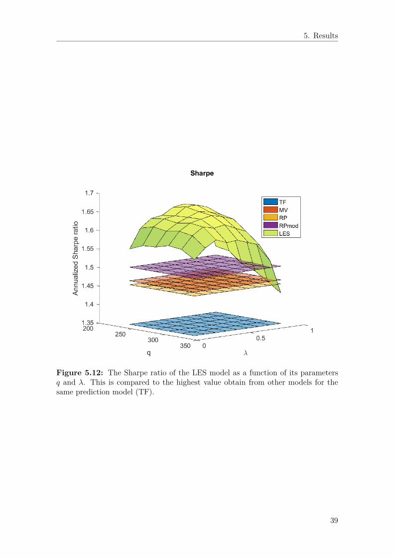
2 . Figure 5.12 shows theSharpe ratio as a function of the time horizon q and the penalty parameter λ. Forcomparison, the best results from previously considered models are included (best inthe sense of the highest Sharpe using this input). The LES model shows a significant

37

5. Results

Figure 5.11: The holding time of the minimum CVaR portfolio as a function ofits parameters q and β, compared to the prediction model TF without portfoliooptimization

boost in Sharpe with reasonably stable results for a range of values on q and λ. Recallthat as λ → 1, the LES model returns the input µ, and note that this figure onlyshows λ-values up to 0.9. Similar results are exhibited for the average drawdown,shown in figure 5.13. This quantity does however appear to be more sensitive tothe number of historical observations, q, for low values on λ. Figure 5.14 shows theresulting holding times and it is clear that LES is a ”faster” model, i.e. has a higherturnover. This will of course reduce the marginal contribution to Sharpe, but thisis not the main problem affiliated with implementing this portfolio method. Thenext section will show that some reformulation of the optimization problem (3.26)is required in order to be well suited for diversified portfolio selection.

38

5. Results

Figure 5.12: The Sharpe ratio of the LES model as a function of its parametersq and λ. This is compared to the highest value obtain from other models for thesame prediction model (TF).

39

5. Results

Figure 5.13: The average drawdown of the LES model as a function of its param-eters q and λ. This is compared to the value obtain from other portfolio models forthe same TF (µ) and the degree of regularization yielding the highest Sharpe in therespective model.

40

5. Results

Figure 5.14: The holding time of the LES model as a function of its parametersq and λ. This is compared to the value obtain from other portfolio models for thesame TF (µ) and the degree of regularization yielding the highest Sharpe in therespective model.

41

5. Results

5.3 Results for different prediction modelsAll previous results has been for portfolio methods applied on one and the sametrend following prediction model. This section will test if the results follow whenvarying this input µ. Recall from section 2.3 that the TF model (µ) was charac-terized by its filter parameter τ describing the considered time horizon. The otherfilter parameters will be kept fixed.

In the previous section the LES model showed stable results for q ∈ [230, 330].Fixating this parameter to the middle point of this interval allows for an easier com-parison. All models should now be evaluated for different TF models (TFτ ) andtheir regularization factor λ ∈ [0, 1]. Figure 5.15 shows the maximum Sharpe ratiofor any value on λ as a function of the TF parameter τ . The observation that themodified RP portfolio outperforms MV and RP in terms of Sharpe appears to holdover the different trading models while MV and RP shows similar performance. Theresults for the LES model stands out as it appears to be almost independent of theinput µ. Unfortunately this is the result of poor diversification, as the LES modelfinds basically the same positions for similar inputs µ which is a terrible propertyfor a portfolio selection method. This feature is shown in figure 5.16 that showsthe average correlation of portfolio returns between models, before (TF) and afterapplying the different methods of portfolio optimization. Obviously the LES modeldestroys all possible diversification from trading different strategies (different TFmodels), unless for λ close to unity for which it returns the input µ. Another ob-servation from figure 5.16 is that both RP models appear to increase diversificationcontrary to the MV model. Excluding the LES model from the remaining results onthe grounds of unacceptable diversification properties, figure 5.17 shows the aver-age drawdown for the degree of regularization λ yielding the highest Sharpe in therespective portfolio model (in other words the value on λ used in figure 5.15). Thisfigure suggests that the MV portfolio will exhibit better drawdown properties thanthe RP models for ”fast” prediction models, i.e. following the shorter trend. Recallthat section 5.1 used a trend following prediction model with TFτ = 200.

For a final reality check, a trading cost will be included in evaluations. Keepingthe unit of returns, the trading cost will be in terms of daily standard deviations ofreturns. The theory behind this is that since the information at time t is used totrade at time t+1, prices can be expected to have moved some amount proportionalto the standard deviation during this time leap (over night). We will examine if themarginal contribution to Sharpe is still positive when adding trading costs and alsoif these costs affect the portfolio models differently. Figure 5.18 shows the highestmarginal Sharpe (for any λ) of the different portfolio models as a function of thetrading cost and the underlying trading model. These results are consistant withprevious analysis as the trading costs affect MV and RPmod in a similar way anddoes not change how these models compare in terms of Sharpe. But as previouslydiscussed the original RP model naturally has a lower holding time and is thus moreaffected by trading costs.

42

5. Results

0 50 100 150 200 250 300 350

1.3

1.4

1.5

1.6

1.7

TF τ

Sharpe

TF MVRP RPmodLES

Figure 5.15: The maximum Sharpe ratio, for any value on λ, as a function of theTF parameter τ .

0.1 0.2 0.3 0.4 0.5 0.6 0.7 0.8 0.9 10.75

0.8

0.85

0.9

0.95

1

λ

Averagecorrelationbe

tweenmod

els

Correlation before/after

TF MVRP RPmodLES

Figure 5.16: The average correlation of returns between trading models, before(TF) and after applying the different methods of portfolio optimization, as a functionof λ.

43

5. Results

0 50 100 150 200 250 300 350−0.44

−0.42

−0.4

−0.38

−0.36

−0.34

−0.32

TF τ

Ann

ualized

Std

Average Drawdown

TF MVRP RPmod

Figure 5.17: The average drawdown, for the value on λ yielding the highest Sharpe,as a function of the TF parameter τ .

MVRP

RPmod

Figure 5.18: The highest marginal Sharpe (for any λ) of the different portfoliomodels as a function of the trading cost and the TF parameter τ .

44

6Discussion

The aim of this thesis has been to compare and improve three existing methods forportfolio optimization, with the main purpose of investigating if alternatives to thestandard mean-variance model could show superior portfolio properties. The Sharperatio of portfolio returns based on historical data has been the primary measure ofperformance followed by the average drawdown of the equity curve defined in section4.2. While the mean-variance portfolio has been criticised for poor performance inpractice, the results in sections 5.1 and 5.3 suggests that this is mainly because ofsensitivity to an ill-conditioned covariance matrix and with a regularized estimatethis model exhibits a positive contribution to both the Sharpe ratio and the averagedrawdown over time. It can thus be considered a very viable option for portfoliosection.

Perhaps the most significant result in this thesis is that the modified RP portfoliosuggested in section 3.2.2 has shown superior performance compared to both MVand the original RP in several central aspects. The results in section 5.3 suggeststhat RPmod exhibits a higher marginal Sharpe for all considered time horizons ofthe underlying prediction model. The drawdown results were however not unam-biguous and suggest that the MV portfolio will have better drawdown properties for”faster” prediction models. But how likely are these results to hold in practice? Thecomparison in section 5.1 considered one underlying prediction model and focusedon investigating the sensitivity of the portfolio performance when varying the otherinput parameters (filter parameters for the variance and correlation estimates). Asthe correlation estimates is a grave approximation of reality, and small changes inthe variance estimate causes small variations in the return series, models for whichthe performance is very sensitive to this input will be likely to perform worse outof sample. The results points to the modified RP portfolio as the most stable tochanges in these inputs considering both the Sharpe ratio and especially the aver-age drawdown, while MV and RP show similar behaviour. This suggests that theobserved performance of RPmod is more likely to hold in practice.

A closer look at how the rolling Sharpe ratio over time compare between the modifiedRP model and MV was investigated in section 5.1.1 and revealed some interestingresults. Risk-parity focuses on allocating risk, and our results show that RPmod ex-hibits almost a consistently lower realized variance of returns while over time keepingan average return very close to that of MV. During shorter periods of time, how theaverage return compares between MV and RPmod will depend on the quality onthe estimated signal strength in which RPmod places less confidence. Evidence has

45

6. Discussion

been found suggesting that there is potential gain to be made from searching for aRPmod portfolio with a high expected return (recall that for M assets there is 2Mportfolios satisfying the RP objective in each time step). Finding the RP portfoliowith the highest expected return is however a non-convex optimization problem.The greedy iteration scheme presented in section 3.2.5 requires modifications to beuseful in practice, the main issue being increased trading costs. Other possibilitiesincludes stochastic optimization algorithms with a well formulated fitness function.

The model from section 3.3.1.3, built upon the framework of minimizing the con-ditional value-at-risk of a portfolio was evaluated in section 5.2 and showed somevery promising results suggesting that this alternative risk measure can contributegreatly to both Sharpe and drawdown properties. However, it turned out that thefinal form of the optimization problem was poorly suited for portfolio selection. Theissue being that the risk term (the sum) of equation (3.26) has a dynamic impacton the solution, having the consequence that with two similar inputs µ the modelreturns the same positions. In practice this will lead to a lack of diversificationwhen trading several different (but similar) prediction models. It may be possibleto counteract this behaviour by enforcing a more strict, explicit constraint on thenorm of the position vector. In other words enforcing that the angle between µand the position vector be smaller than some suitable constant. Further work couldfocus on reformulating the ADMM algorithm in section 3.3.1.4 to fit this purpose.

46

Bibliography

[1] Andreasson, N., Evgrafov, A., Patriksson, M., Gustavsson, E., andOnnheim, M. Introduction to Continuous Optimization. Edition 2 : 1. Stu-dentlitteratur AB, 2013.

[2] Boyd, S., Parikh, N., Chu, E., Peleato, B., and Eckstein, J. Dis-tributed optimization and statistical learning via the alternating directionmethod of multipliers. Foundations and Trends in Machine Learning 3, 1 (Jan.2011), 1–122.

[3] Cont, R. Empirical properties of asset returns: stylized facts and statisticalissues. Quantitative Finance 1 (2001), 223–236.

[4] Ledoit, O., and Wolf, M. A well-conditioned estimator for large-dimensional covariance matrices. Journal of Multivariate Analysis 88, 2 (2004),365 – 411.

[5] Lee, W. Risk-Based Asset Allocation: A New Answer to an Old Question?The Journal of Portfolio Management (June 2011), 11–28.

[6] Markowitz, H. Portfolio selection. The Journal of Finance 7, 1 (1952),77–91.

[7] Mestre, X. Improved estimation of eigenvalues and eigenvectors of covari-ance matrices using their sample estimates. IEEE Transactions on InformationTheory 54, 11 (Nov 2008), 5113–5129.

[8] Qian, E. Risk parity portfolios: Efficient portfolios through true diversifica-tion. Panagora Research Paper (September 2005).

[9] Rockafellar, R. T., and Uryasev, S. Optimization of conditional value-at-risk. Journal of Risk 2 (2000), 21–41.

[10] Sébastien Maillard, T. R., and Teïletche, J. The properties of equallyweighted risk contribution portfolios. The Journal of Portfolio Management 36,4 (2010), 60–70.

[11] Yang, D., and Zhang, Q. Drift-independent volatility estimation based onhigh, low, open, and close prices. Journal of Business 70, 3 (2000), 477–491.

47

Bibliography

48

portfolio optimization with trend following strategies

Documents