core network optimization and resiliency strategies

!!!!

!!!!!!!!!

D"7.6"

Core" network" optimization" and"resiliencey"strategies"!!

Dissemination!Level:!!!!

• Dissemination!level:!PU!=!Public,!RE! =! Restricted! to! a! group! specified! by! the! consortium! (including! the!Commission!Services),!PP! =! Restricted! to! other! programme! participants! (including! the! Commission!Services),!CO! =! Confidential,! only! for! members! of! the! consortium! (including! the!Commission!Services)!

!!

08!Fall$

08!The$,$$

! !!

FP7!–!ICT!–!GA!318137! ii!DISCUS!!!

!

!

!

!Abstract:!This! deliverable! describes! the! optimization! models! and! methods! that! are!needed!in!order!to:!(i)!optimize!the!design!and!operation!of!the!DISCUS!core!network,!and!(ii)!guarantee!that!the!DISCUS!architecture!is!able!to!guarantee!to! the! provisioned! services! survivability! in! the! presence! of! core! network!element!failures.!

The!work!presented!in!the!document!is!divided!into!three!main!parts.!In!the!first!one!the!document!starts!by!introducing!a!framework!for!evaluating!the!hardware!cost!(i.e.,!Chapter!2).!This!information!is!subsequently!used!as!the!basis! for! the! design! of! single! and! multilayer! core! network! solutions! (i.e.,!Chapter!3! and!4).!The! second!part! of! the!deliverable! (i.e.,! Chapter!5! and!6)!focuses!more! on! the! network! in! operation,! i.e.,! it! addresses! the! problem!of!providing! survivability! against! failures! of! core! network! elements! in! the!presence! of! dynamic! traffic.! The! last! part! of! the! deliverable! addresses! two!additional!aspects!related!to!reliability.!Chapter!7!provides!an!insight!on!what!is! the! impact! of! energy! saving!mechanisms! on! the! lifetime! of! core! network!devices,! while! Chapter! 8! introduces! a! control! architecture! that! can! be!implemented!to!support!fast!and!accurate!reaction!to!failures.!

!

!

! !!

FP7!–!ICT!–!GA!318137! iii!DISCUS!!!

!COPYRIGHT!

© Copyright by the DISCUS Consortium. The DISCUS Consortium consists of: Participant Number

Participant organization name Participant org. short name

Country

Coordinator 1 Trinity College Dublin TCD Ireland Other Beneficiaries 2 Alcatel-Lucent Deutschland AG ALUD Germany 3 Nokia Siemens Networks GMBH & CO. KG NSN Germany 4 Telefonica Investigacion Y Desarrollo SA TID Spain 5 Telecom Italia S.p.A TI Italy 6 Aston University ASTON United

Kingdom 7 Interuniversitair Micro-Electronica Centrum

VZW IMEC Belgium

8 III V Lab GIE III-V France 9 University College Cork, National University of

Ireland, Cork Tyndall & UCC Ireland

10 Polatis Ltd POLATIS United Kingdom

11 atesio GMBH ATESIO Germany 12 Kungliga Tekniska Hoegskolan KTH Sweden

This document may not be copied, reproduced, or modified in whole or in part for any purpose without written permission from the DISCUS Consortium. In addition to such written permission to copy, reproduce, or modify this document in whole or!part, an acknowledgement of the authors of the document and all applicable portions of the copyright notice must be clearly referenced. !All rights reserved.

! !!

FP7!–!ICT!–!GA!318137! iv!DISCUS!!!

Authors: (in alphabetic order)

Name Affiliation

Norbert Ascheuer ATESIO

Oscar Gonzalez de Dios TID

Marija Furdek KTH

Victor Lopez TID

Deepak Mehta UCC

Paolo Monti KTH

Avishek Nag TCD

Barry O'Sullivan UCC

Cemalettin Ozturk UCC

Luis Quesada UCC

Christian Raack ATESIO

Lena Wosinska KTH

Internal reviewers:

Name Affiliation

Andrea Di Giglio TI

Marco Ruffini TCD

Due!date:!!30.04.2015!

Contents

1 Introduction 3

2 Cost modeling 62.1 Electronic switching at the MC node . . . . . . . . . . . . . . . . . . . . . . 72.2 Photonic switching at the MC node . . . . . . . . . . . . . . . . . . . . . . . 92.3 Fiber link cost . . . . . . . . . . . . . . . . . . . . . . . . . . . . . . . . . . . 112.4 A dimensioning exercise . . . . . . . . . . . . . . . . . . . . . . . . . . . . . 12

3 Multi-layer network design 143.1 DISCUS layers . . . . . . . . . . . . . . . . . . . . . . . . . . . . . . . . . . 153.2 The DISCUS architecture: Optical islands . . . . . . . . . . . . . . . . . . . 163.3 Data: MC node distributions, cable networks, traffic matrices . . . . . . . . 173.4 Solution methodology . . . . . . . . . . . . . . . . . . . . . . . . . . . . . . 203.5 Computations . . . . . . . . . . . . . . . . . . . . . . . . . . . . . . . . . . . 263.6 Conclusion . . . . . . . . . . . . . . . . . . . . . . . . . . . . . . . . . . . . 29

4 Resilient core network planning 314.1 Resilient core network design . . . . . . . . . . . . . . . . . . . . . . . . . . 324.2 Resilient core network dimensioning using M/C nodes based on synthetic

programmable ROADMs . . . . . . . . . . . . . . . . . . . . . . . . . . . . . 444.3 Protection of the core network in the presence of physical-layer attacks . . 494.4 Resilience strategies based on dual homed M/C nodes . . . . . . . . . . . 604.5 Conclusion . . . . . . . . . . . . . . . . . . . . . . . . . . . . . . . . . . . . 64

5 Resilient service provisioning 675.1 Survivability Strategies WDM Networks Offering High Reliability Performance 675.2 Dynamic Provisioning Utilizing Redundant Modules in Elastic Optical Net-

works Based on Architecture on Demand Nodes . . . . . . . . . . . . . . . 725.3 Restoring Optical Cloud Services with Service Relocation . . . . . . . . . . 765.4 Conclusions . . . . . . . . . . . . . . . . . . . . . . . . . . . . . . . . . . . . 80

6 Survivable Optical Metro/Core Networks with Dual-Homed Access: an Avail-ability vs. Cost Assessment Study 816.1 Reference Architecture . . . . . . . . . . . . . . . . . . . . . . . . . . . . . . 826.2 Network Design And Control Plane Algorithms . . . . . . . . . . . . . . . . 836.3 Case study . . . . . . . . . . . . . . . . . . . . . . . . . . . . . . . . . . . . 866.4 Results . . . . . . . . . . . . . . . . . . . . . . . . . . . . . . . . . . . . . . 866.5 Conclusions . . . . . . . . . . . . . . . . . . . . . . . . . . . . . . . . . . . . 89

FP7-ICT-GA 3181371

7 Impact of Energy-Efficient Techniques on a Device Lifetime 90

7.1 Impact of Sleep Mode Operations on a Device Lifetime . . . . . . . . . . . . 91

7.2 EDFA Failure Rate Model and Average Failure Rate Acceleration Factor . . 92

7.3 Case Study . . . . . . . . . . . . . . . . . . . . . . . . . . . . . . . . . . . . 94

7.4 Conclusions . . . . . . . . . . . . . . . . . . . . . . . . . . . . . . . . . . . . 98

8 Control plane interaction for resilience scenarios 99

8.1 DISCUS control plane architecture . . . . . . . . . . . . . . . . . . . . . . . 99

8.2 Centralised vs. distributed resilience mechanism . . . . . . . . . . . . . . . 100

8.3 Impact of a centralized or distributed control plane in DISCUS . . . . . . . . 102

8.4 Performance analysis of DISCUS control plane . . . . . . . . . . . . . . . . 104

8.5 Comparison between both approaches . . . . . . . . . . . . . . . . . . . . . 106

8.6 Conclusions . . . . . . . . . . . . . . . . . . . . . . . . . . . . . . . . . . . . 109

9 Conclusions 110

A Acronyms 111

B Versions 113

FP7-ICT-GA 3181372

Chapter 1

Introduction

Optical networks are exposed to a wide range of failures affecting single or multiple networkcomponents and disturbing a multitude of connections, possibly over greater geographi-cal area. Failures can be caused, for example, by physical damage to the infrastructure- accidental optical fiber cuts due to construction work are the leading cause of networkdisruptions. Fatigue, mishandling, or environmental shocks can also result in faults of net-work components and devices. Aside from individual component failures, entire nodes canbecome disabled due to weather conditions, power outages, or natural disasters. Further-more, the network infrastructure can also be targeted by malicious actions attempting todisrupt service or gain unauthorized access to information.

Due to the extremely high data rates and traffic volumes carried, nation-wide core networksmust be able to provide quick and efficient recovery of affected connections. In order toguarantee service survivability in the presence of failures, network resilience must be takeninto account both in the network design and during operation. In addition to be consideredfor deployment by the operators, the developed resiliency schemes must maintain highcost- and resource-efficiency.

The goal of this deliverable is to investigate means of increasing network resilience undera wide range of failures through judicious network design and connection provisioning instatic and dynamic traffic scenarios. To be able to do so, it is necessary to first establish aframework for evaluating the hardware cost which then serves as the basis for network de-sign. Network design further needs to consider the specific constraints of different networklayers as well as interactions between the layers, leading to a very complex integrated plan-ning problem. Furthermore, the control plane needs to support fast and accurate reactionto failures by triggering appropriate recovery mechanism.

Network resilience approaches in general rely on providing additional capacity in the net-work to be used as backup during failures. During network design, this redundancy canbe provided by setting up the interconnections between nodes in a way which ensuresthe existence of physically disjoint routes through the network between all pairs of nodes.This means that additional physical links need to be set up in the network which are notvital to ensure connectivity under normal operating conditions, but are crucial to maintainconnectivity in the event of failure. Due to the large sizes of the network, deciding whichlinks to add while keeping the cost at a minimum and satisfying the signal reach entails acomplex optimization procedure.

Redundant backup paths in the network which protect the primary paths of connectionswhen they are affected by failures can be pre-planned, which is the underlying principle ofprotection approaches, or can be reserved dynamically, upon a failure, which is inherent forrestoration. Protection strategies in the DISCUS topology can utilize the dually-homed ac-cess segment to obtain high connection availability under lower resource usage comparedto the single-homing scenario. One of the goals of the work presented in the deliverablewas to estimate the capacity overshoot needed to provide survivability in the dually-homedDISCUS reference topology when different design approaches are applied. In other words,

FP7-ICT-GA 3181373

it is important to understand how much overprovisioning (in terms of extra WDM transpon-ders) is needed to obtain a favourable tradeoff between resource usage and connectionsurvivability.

Protection and restoration strategies can also be combined into a hybrid approach toachieve a resource-efficient increase of network resiliency under overlapping failures ofmore than one link. Under dynamic scenarios, resilience of optical cloud services can sig-nificantly benefit from the concept of service relocation, where the service is moved fromone data center to another in the occurrence of a failure to allow for greater flexibility inbackup path provisioning.

Survivability from failures of node components can take place at the node level as wellwithout triggering network level recovery, provided that redundant components are placedinside the node and that the node architecture supports flexible operation. ReconfigurableAdd Drop Multiplexers (ROADMs) implemented by Architecture on Demand (AoD) repre-sent a promising approach for this functionality which could alleviate the resource con-sumption burden of failure recovery at the network level.

Survivability approaches which protect from component failures might not provide protec-tion from deliberate, attack-like events in the network because both the primary and thebackup path might be affected by the attack. Thus, such approaches need to identify thepotential risk of the primary and backup path of connections being simultaneously affectedby an attack and establish the paths in a way which reduces that risk, while maintainingresource-efficiency of conventional, failure-protection approaches.

Finally there is additional survivability aspect that is important to highlight, i.e., the impactof energy saving mechanisms on the lifetime a device. In fact a possible drawback of agreen approach is that frequent on/sleep switching may negatively impact the failure rateperformance of a device, and consequently increase its reparation costs. In particular, it isimportant to make sure that the potential savings brought by a reduced power consumptionlevel are not lower than possible extra reparation costs caused by a reduced lifetime.

While some of the survivability approaches presented in this document focus on the DIS-CUS reference topology, others have been tested on a variety of reference topologies fromthe literature in order to gain a comprehensive insight into their behaviour. This thoroughassessment of their performance will allow us to select the most promising approaches forthe consolidated network design. This deliverable is organized as follows.

Chapter 2 provides a consolidated model of cost and hardware including core photonicswitching, signal regeneration and Raman amplification. A dimensioning exercise is alsoprovided to provide insight into optimization model parametrization.

The detailed model presented in Chapter 2 then serves as the basis for multi-layer net-work design study given in Chapter 3. Instead of adopting a common bottom-up approachof decoupling different network layers, which may lead to sub-optimal results, the work inChapter 3 follows an integrated approach which allows for greater flexibility during opti-mization of the virtual topology and installation cost.

Chapter 4 focuses on resilient network planning by first incorporating resilience and signalreach constraints into network design. The work further investigates methods of providingnode-level recovery of component faults in synthetic programmable ROADMs implementedby AoD, proposes an approach for dedicated path protection which minimizes the numberof connections unprotected from physical-layer attacks aimed at service disruption, andstudies the benefits of utilizing dual homing in protection from core link failures.

FP7-ICT-GA 3181374

Chapter 5 investigates a hybrid approach for resilient service provisioning which combinespath protection with path restoration. It then analyzes the benefits of placing redundantmodules inside AoD-based ROADMs in achieving a beneficial tradeoff between connectionavailability and cost. Further, it develops an approach for restoring optical cloud servicesbased on service relocation.

Chapter 6 deals with the problem of finding a favourable tradeoff between network overdi-mensioning and the resulting network survivability performance.

Chapter 7 investigates how energy saving mechanisms based on frequent on/sleep switch-ing may impact the failure rate (i.e., lifetime) performance of a device.

Chapter 8 presents the interaction of the control plane in resilience mechanims in central-ized and distributed scenarios.

FP7-ICT-GA 3181375

Chapter 2

Cost modeling

Figure 2.1: Cost evaluation based on network dimensioning. Simplified MC-node model:MPLS-TP, IP, and Photonic switching. IP functionality is needed only for service nodes such asfor data centers (DC) and internet exchanges (IX). For optimization we simplify and assume asingle MPLS-TP, a single IP, and a single Polatis switch. This is feasible as most of the costcomes from the port count.

In this chapter, we will introduce a cost and hardware model that we will use for any op-timization related to the core network. This cost model is an extension of the tentativemodel presented in Deliverable D2.6 [6]. Starting from the model in [6], we mainly consol-idated the cost for core photonic switching and added a model for signal regeneration andRaman amplification. Our model is in large parts based on the capex-models developed inthe IDEALIST project, see [3]. We adapted the model following the DISCUS architecture. Inparticular we add cost values for the Polatis switch (see [8]) as well as for Raman amplifiersand the flex-grid signal types used within DISCUS (see [4, 10]). The flex-grid transpondermodel has been consolidated compared to Deliverable D2.6 [6].

Recall that this hardware model is designed to be used for optimization, that is, toparametrize objective functions of optimization models and to evaluate the cost of opti-mization solutions. In this respect, it only reflects a coarse view on the capital expenditureswith a clear focus on the main cost-drivers. It cannot replace a detailed cost and cash-flowanalysis. Such an analysis will be reported in Deliverable D2.8 [11].

As already mentioned in [6], for optimization it is feasible to ignore any cost that is indepen-dent of the solution, e.g. cost that is proportional to the number of customers, a constant.

FP7-ICT-GA 3181376

In many cases, it is even feasible to further simplify and combine network elements toblocks of equipment introducing the notion of link or node designs. This will be done forinstance with the core photonic switching elements below similar to what has been donein [82] and [3].

Tables 2.1, 2.2, and 2.3 present our cost and hardware model for electronic switching andphotonic switching at the MC node, and for the Core fiber link, respectively. All cost valuesare given both in EUR and in the IDEALIST cost unit (ICU), where

1 ICU = e 50,000. (2.1)

defines the conversion factor used.

All interfaces in this chapter are bidirectional. Even if we speak of a fiber line interface inthe following, or simply a fiber we refer to a fiber pair in reality (one fiber for each direction).

2.1 Electronic switching at the MC node

The MC node hardware model in Table 2.1 provides cost values for the electronic switchingelements at the MC node, see [7] and Figure 2.2.

As mentioned above, we partially made use of the models developed in the IDEALISTproject and published in [3]. We reuse the 2015 models for IP-MPLS (router, cards) andMPLS-TP (switches, cards) with a restriction to 400G slot capacities and 40G, 100G, and400G ports.

Type Provides Cost in e Cost in ICU

IP-MPLS router 16 400G Slots 215,000 4.300032 400G Slots 1,143,500 22.8700· · · · · · · · · · · ·

1152 400G Slots 416,451,000 8329.0200· · · · · · · · · · · ·

IP-MPLS card 10 40 GE ports 128,000 2.56004 100 GE ports 144,000 2.88001 400 GE port 137,000 2.7400

MPLS-TP switch, 400G slots 16 400G Slots 192,000 3.840032 400G Slots 384,000 7.6800· · · · · · · · · · · ·

112 400G Slots 1,344,000 26.8800· · · · · · · · · · · ·

MPLS-TP line-card 10 40G ports 43,360 0.86724 100G ports 54,200 1.08401 400G port 60,680 1.2136

Transceiver, Grey, Short Reach 1 40G port 400 0.00801 100G port 1,600 0.03201 400G port 4,000 0.0800

Table 2.1: MC-node hardware and cost model based on the values defined in [82] and [3].We added OLT cards for MPLS-TP switches with a cost based on the cash-flow modeling inWP2 (8 port card has been scaled to 40 port card).

FP7-ICT-GA 3181377

The node model assumes the L2, L3 routing and switching elements to be organized inthree levels: chassis, cards, and transceivers, see [6, Figure 20]. The chassis is character-ized by its capacity in terms of slots, the cards in terms of throughput and type and numberof ports, and the interfaces in terms of their client rate. Line-Cards are supposed to re-quire one slot in the chassis. We assume 400G slots for IP-MPLS as well as MPLS-TP.All cards may be equipped with short reach transceivers which in turn can be connectedto transponders. We do not assume colored long reach transceivers here for simplicity.In fact, we may assume a colored interface at the cost of a short reach interface plus atransponder. For the cost of transponders see the optical equipment below.

Type Provides Reach Cost in e Cost in ICU

Polatis Switch 100 Fiber ports 17,063 0.3413· · · · · · · · · · · ·

400 Fiber ports 34,650 0.6930· · · · · · · · · · · ·

Fixed Grid

Transponder 1 40G port 2500 km 24,000 0.48001 100G port 2000 km 50,000 1.00001 400G port 150 km 68,000 1.3600

WDM Terminal 1 Fiber port 48,000 0.9600(AWG+Interleaver+OLA)

Flexible Grid

Transponder 1 40G port 2430 km 47,500 0.95001 2x100G port 2430 km 150,000 3.00001 100G port 1170 km 50,000 1.00001 2x100G port 500 km 55,000 1.10001 400G port 1170 km 150,000 3.00001 2x400G port 500 km 160,000 3.2000

WDM Terminal 1 Fiber port 78,000 1.56(WSS + OLA)

Add Drop Block 16 Add Drop ports 32,000 0.64

Table 2.2: Hardware and cost model for optical core equipment. We assume regeneratorsat the cost of 1.6 times the corresponding transponder. Regenerators double the reach ofthe respective signal. The cost values for WDM terminals combine cost numbers from theIDEALIST model [3], which states 1 OLA = 0.3 ICU, 1 WSS (1x20/20x1) = 0.48 ICU, 1 AWG =0.07 ICU, and 1 Interleaver = 0.04 ICU.

We will assume MPLS-TP switches at all MC nodes. For simplicity, in optimization wewill not distinguish core-side and access-side switches. IP-MPLS routers exist only atservice nodes, that is, IP-nodes of service providers (SP), data-center (DC), or internetpeering points (internet exchanges, IX) see [6, Section 2.3] and Figure 2.1 compared toFigure 2.2(b). We remark that IP-routers with a slot count of more than 16 are multi-chassisrouters. There is a significant cost increase from the single chassis router (16 slots) to the2-chassis router with 32 slots. However the cost for larger routers then increases roughlylinearly and can be computed with a simple formula based on the number of required slots,see [3] and [82].

FP7-ICT-GA 3181378

(a) Switching using Optical Cross Connected based on WSS line inter-faces

(b) Switching using AWG based Mux/Demux and the Polatis switch

Figure 2.2: Two options for core photonic switching

2.2 Photonic switching at the MC node

Table 2.2 aims at providing the optical switching hardware and cost. As explained in detailin [8] and [12] there are two options for core photonic switching at the MC node compatiblewith the DISCUS architecture.

WSS line interfaces

Option (a) as indicated in Figure 2.2(a) and 2.3 is available for both flex-grid and fixed-gridWDM. It is based on optical cross connects built from WSS (wavelength selected switches)and Add/Drop blocks with 16 Add/Drop ports each. In this case, the Polatis switch isnot needed for switching core-to-core lambdas. It is used only to have more flexibility inswitching wavelength services between the access network and the core network. We willrefer to the fiber terminating elements as WDM terminals. These include the switches andamplification. For Option (a) it holds:

1 WDM Terminal = 2 WSS + 2 OLA. (2.2)

We have to provide 1 WDM Terminal for every fiber line interface at the MC node. In ad-dition we need an appropriate number of Add/Drop ports, one for each terminated lambda

FP7-ICT-GA 3181379

Figure 2.3: 2-degree core photonic switch based on (flex-grid) WSS line interfaces

channel. If f is the number of fiber ports and n the number of terminating channels, thenthe cost of the core photonic switching element for Option (a) amounts to

1.56 · f + 0.64 · d n16e ICU, (2.3)

where 1.56 is the ICU cost for on WDM terminal based on WSS and 0.64 is the cost inICU for one Add/Drop block with 16 ports. If n is the number of terminating channels, thenwe need

npolatis = 2 · n (2.4)

ports at the Polatis switch.

AWG Mux/Demux and Polatis switch

Option (b) for photonic switching as indicated in Figure 2.2(b) is based on AWG Mux/De-mux elements to (de)multiplex the WDM signals and the Polatis switch to cross-connect theindividual lambda signals. However, this option with relatively moderate switching cost isavailable only for fixed-grid WDM systems. Again we refer to the fiber terminating elementincluding amplification as WDM terminal. In case of Option (b) we have:

1 WDM Terminal = 4 AWG + 2 OLA + 2 Interleaver. (2.5)

We have to provide 1 WDM Terminal for every fiber line interface at the MC node and noadditional Add/Drop blocks. Instead an appropriate number of ports at the Polatis switchhave to be provided. If f is the number of fiber ports and n the number of terminatingchannels, then we need

npolatis = 176 · f + 2 · n (2.6)

ports at the Polatis switch. The single-sided Polatis switch has cost

0.0224 + npolatis · 0.00118 ICU, (2.7)

where npolatis is the number of fiber ports at the Polatis switch. We will assume the Polatisswitch to be used for access side and core side switching.

FP7-ICT-GA 31813710

Type Provides Cost in e Cost in ICU Unit

Duct Duct-Space 66,300 1.3260 Km

Cable 276 Fibers 7,859 0.1572 KmCable 240 Fibers 7,145 0.1429 KmCable 192 Fibers 6,145 0.1229 KmCable 144 Fibers 5,145 0.1029 KmCable 96 Fibers 4,145 0.0829 KmCable 48 Fibers 3,145 0.0629 KmCable 24 Fibers 2,716 0.0543 KmCable 12 Fibers 2,430 0.0486 Km

Raman amplifier 80 km Raman amplifier 30,000 0.6000 Piece

Optical Line Amplifier (OLA) 80 km EDFA amplifier 15,000 0.3000 Piece

Digital Gain Equalizer (DGE) 320 km equalizer 8,000 0.1600 Piece

Table 2.3: The cost per km of each individual fiber is between e 28 (276-fiber cable) ande 43.0 (96-fiber cable). Ignoring smaller cables it may hence be feasible to assume an averagefiber cost of e 40.0 per km.

Transponders and regeneration

Transponders (Fixedgrid and Flexgrid) are used on both sides of every core optical channelin combination with a short-reach transceiver interface at the MPLS-TP (or IP) switches.Depending on the signal, transponders have a certain signal-reach, see Table 2.2. Thereach can be extended by regenerating the signal at the MC node (after add/drop) whichis done using regenerators. Each transponder has a corresponding regenerator, whichallows to regenerate the signal without going to the electrical switches. That is, the use of aregenerator doubles the reach of the respective signal types. We will assume regeneratorsto have a cost of 1.6 times the cost of the corresponding transponder.

Some of the transponders in Table 2.2 provide 2 client interfaces doubling the bitrate ca-pacity. Clearly, these need two transceivers on each side.

2.3 Fiber link cost

For most of the studies in this Deliverable we assume spare dark fiber to be available tothe operators at no installation cost. However, even in the spare fiber scenario using a corefiber incurs cost. First of all Optical Line Amplifiers (OLA) have to be provided every 80kilometers and secondly, Digital Gain Equalizers (DGE) are needed every 320 kilometersof the fiber span. OLAs and DGE are already provided at all network nodes (included inthe cost for WDM Terminals, see above). That is, a fiber with length k km between two MCnodes incurs a cost of

0.3 · b k80c+ 0.16 · b k

320c ICU, (2.8)

according to the cost for OLA and DGE in Table 2.3. Moreover, notice that the cost for linetermination can be mapped to the fiber cost in all optimization models. That is, for eachindividual fiber, the cost for two WDM terminals (one on each end) can be added to thecost for OLA and DGE.

FP7-ICT-GA 31813711

If instead a green-field scenario is considered we add cable installation and duct build cost.For cable installation we use the values provided by Table 2.3, which are identical to thoseused for the backhaul and E-side of the DISCUS network, see [6]. In addition we assume aduct build probability of 5%, that is, for each used fiber link in the network (independent ofthe number of fibers in use) we assume 5% of e 66,300 = e 3,315 per km duct build cost.

2.4 A dimensioning exercise

In the following we will use the introduced hardware and cost model to dimension theequipment of a single MC node. This helps us understand how to parametrize the objectivefunctions of our optimization models.

Independent of the actual hardware and cost-model, the outcome of an optimization of theaccess network is the number of LR-PONs connected to every MC node. In fact, for corenetwork optimization, we start from a given set of MC node locations with already con-nected customers and LR-PONs. Similarly, core network optimization returns the numberof terminating fibers and the number of terminating channels at the MC node (independentof hardware and cost).

It turns out that the main cost incurring at an arbitrary MC node can be estimated startingfrom these three figures: (i) connected LR-PONs, (ii) terminating fibers, and (iii) terminatingchannels, see Figure 2.1.

Let us first assume the considered MC node does not provide data center or peering pointservices as the one in Figure 2.1. Let us further assume that optimization returns thefollowing figures for one of the MC nodes:

• p connected LR-PONs

• f connected fibers

• n400

400G channels, n100

100G channels, n100

40G channels.

In this case the cost of the MC node is estimated by counting the necessary networkelements as follows. Electronic equipment depends on the number and type of terminatedchannels (core side) and the number connected LR-PONs. Transceivers, line-cards, and

Element Number

40G transceiver n40

100G transceiver n100

400G transceiver n400

40G MPLS-TP line-card c40 = dn4010 e

100G MPLS-TP line-card c100 = dn1004 e

400G MPLS-TP line-card c400 = n400

OLT line-card c40 = d p40e

400G MPLS-TP slots c40 + c100 + c400 + c40

Table 2.4: Dimensioning: Electronic equipment at the MC node for fixed-grid WDM

FP7-ICT-GA 31813712

the MPLS-TP switch are dimensioned accordingly. The resulting dimensioning of the MCnode electronics can be found in Table 2.4.

For the optical equipment we have to count the transponders necessary to terminate thechannels and the WDM terminals to terminate the fibers. In addition the Polatis switchhas to be dimensioned based on the number of fibers and channels. See Table 2.5 andTable 2.6 for the resulting dimensioning of the MC node optics for fixedgrid and flex-gridWDM systems, respectively. Recall that in case of flex-grid WDM systems the count ofthe Polatis switch ports changes as well as the cost for the WDM terminal. In addition, wehave to provide an appropriate number of Add/Drop blocks, see Table 2.6.

Element Number

WDM Terminal (AWG) f

40G transponder fixed grid n40



Polatis switch fiber ports p+ 176f + 2(n40 + n100 + n400)

Table 2.5: Dimensioning: Optical equipment at the MC node for fixed-grid WDM

Element Number

WDM Terminal (WSS) f

Add/Drop blocks d (n40+n100+n400)16 e

40G transponder flex-grid n40



Polatis switch fiber ports p+ 2(n40 + n100 + n400)

Table 2.6: Dimensioning: Optical equipment at the MC node for flex-grid WDM

Based on these device counts and the cost values in Table 2.1 and 2.2 we can easilyprovide a reasonable estimate for the cost of a single MC node. Notice that for the costof the transponders we need to know the actual signal type in addition to the count of theinterfaces. To determine the total cost of the core network we aggregate the cost at allMC nodes and add the cost for fibers following the remarks above and values provided inTable 2.3.

FP7-ICT-GA 31813713

Chapter 3

Multi-layer network design

In this chapter, we will study the cost and scalability of core networks based on the opticalisland concept. In particular, we will compare optical islands with hierarchical architectureconcepts that are based on grooming traffic before entering a smaller inner core network.We will prove that optical islands are future-proof in the sense that they are the most cost-effective with respect to increasing traffic volumes. For selected network scenarios, we willalso present the traffic volume threshold above which optical islands are less expensivethan grooming architectures. All cost values are based on the cost model presented inChapter 2.Before we show our computational results and findings we have to introduce the requiredmathematical concepts and algorithmic machinery.

Figure 3.1: Client-Server relation in multi-layer networks: Links of the (virtual) client layer arerealized by paths in the (physical) server layer. Each of the paths consumes capacity in theserver.

In practice, telecommunication core networks consist of a stack of technologically differ-ent network layers, which are embedded into each other following a client-server relation.In the following we will think of client layers being ’on top’ server layers. The links of aclient layer can be seen as requests or demands. These request are realized by paths inthe server layer. The server layer has to provide the necessary capacities. The realizedcapacities form links in the server layer, which in turn become requests for the next under-lying network layer in the stack. In this respect each layer may be server and client at thesame time.Each layer is defined by its provided capacity unit (to realize requests from the above client)and its consumed capacity unit (the request to the next layer below). Typical capacity unitsare Gbps, channel, fiber, cable, ducts. Capacities are typically provided as multiples ofa base unit, e.g. multiples of 40, 100, 400 Gbps, or multiples of 88-slot DWDM systems(fibers). Each layer may also restrict the possible realization of its demands, e.g. it may

FP7-ICT-GA 31813714

Layer Provides capacity Requests capacityin terms of in terms of

Service Traffic in Gbps

Virtual Gbps (40G, 100G, 400G) Channel slots (1,2,4)

Physical Channel slots (88, 120) Fibers

Cable Fibers Ducts

Duct Ducts Trenches

Trench Trenches

Table 3.1: The network layer structure with provided and consumed resources. For corenetwork design we will ignore Trench and Duct layer and assume the Cable layer with sparefibers to be given.

force a single path realization instead of a splitting of the request across multiple paths. Itmay also claim a certain level of survivability of the realization of its requests.

This strong coupling of capacities embedded in capacities across multiple layers yields oneof the most challenging dimensioning problem in combinatorial optimization often calledmulti-layer network design: The task is to dimension all network layers in such a way thatall requests can be realized across all layers, while minimizing the cost for all resources.We refer to [72] for a detailed mathematical analysis of the structure of the two-layer versionof this problem, also see [77].

3.1 DISCUS layers

From a schematic and mathematical point of view we may distinguish the following networklayers within the DISCUS core network:

Service layer

Based on the traffic modeling in Deliverable D2.4 [5], Deliverable D2.6 [6] and D2.8 [11](forthcoming) we may assume that we are given a demand matrix that defines for each pairof MC nodes a traffic demand in Gbps. At this point we aggregate the traffic for differentservice characteristics (internet exchange traffic, data center traffic, peer-to-peer traffic)to a single service link. A service link is realized by paths in the underlying electronicswitching layer and consumes Gbps.

Virtual layer

For simplicity, we will refer to the electronic switching layer (IP/MPLS-TP) as the virtuallayer. The virtual layer provides capacity in terms of 40Gbps 100Gbps, or 400Gbps links,see the hardware and cost model 2. Each virtual link (a 40G,100G, or 400G link) depend-ing on the signal type (the modulation format) requests a certain channel slot capacity inthe underlying physical fiber layer. The individual slot demands of each signal type arestated in [10, Table 1].

FP7-ICT-GA 31813715

Physical layer

For simplicity, we will refer to the optical transport, WDM or fiber layer as the physical layer.The physical layer provides channel slot capacity in terms of fibers. In fixed grid scenarioswe assume fibers with 88 slots. In flex-grid scenarios a fiber has 120 slots (37.5 GHzspacing), see [4]. Fibers consume cable capacity.

Cable, duct, and trenching layers

The cable deployment layer provides fiber capacity. We distinguish cables of differentsizes, see Table 2.3. Clearly, cables need duct space. The duct layer provides cablecapacity and might need trenching.

The different layers and their resources are summarized in Table 3.1. Throughout the restof this section we will ignore trench capacities and duct capacities. We will further assumethe core cable layer with spare fibers to be given as input, see below. That is, we willconcentrate on the design of the virtual and the physical layer based on a given trafficmatrix (the service layer), which is a two-layer network design problem.

3.2 The DISCUS architecture: Optical islands

Metro-core node 1 Metro-core

node 2

Metro-core node 4Metro-core

node 3

Metro-core node 7


node 8

Metro-core node 5

Metro-core node 6Physical

cable routes

Optical channels(wavelengths)

Form logical mesh of interconnects

Optical Island

Metro-core node 1 Metro-core

node 2


node 3

Metro-core node 7


node 8

Metro-core node 5

Metro-core node 6Physical

cable routes

Optical channels(wavelengths)

Form logical mesh of interconnects

Optical Island

Figure 3.2: Optical islands: The cable links (with spare fibers) are in blue. The colored pathsare optical channels, that is, virtual links and their realizations in the fiber layer. In the opticalisland concept we assume that each service link is realized by direct virtual links (single-hopvirtual paths). It follows that the virtual layer becomes a full-mesh of optical channels. In thisfigure we see only a subset of the necessary virtual links.

In most practical situations there is a serious of constraints to be taken into account withrespect to the layer structure. In particular there are restrictions on the allowed path real-izations of a given client link. The DISCUS architecture introduces the following constraintson the client link realizations:

FP7-ICT-GA 31813716

• Service link realizations: In a pure optical island, each service link is realized as asingle-hop virtual path. That is, the service traffic between two MC nodes is sentdirectly using a direct optical channel connection (or multiple such channels). Withthis definition of an optical island there is an optical channel for each service link.Since we expect a service link (a demand) for each pair of MC nodes, the virtuallayer becomes a full-mesh network. This results in a strong restriction on the pos-sible virtual topologies and network architectures. Below we will study under whichconditions this solution is cost-effective. In particular, we will compare optical islandswith architectures that allow for grooming at intermediate MCs and their MPLS-TP orIP switches. Grooming may take place at all inner nodes of a virtual path.

• Virtual link realizations: Optical channels (virtual links) are realized as paths in thephysical fiber layer. For these realizations there is a reach limit coming from the signaltypes and the corresponding transponders. Within DISCUS we assume 3 signal-typeswith reaches of 500km (400G), 2000km (100G), and 2500km (40G) for fixedgrid sys-tems and 6 signal-types with reaches between 500 and 2430km for flex-grid systems.To realize an optical channel with a certain capacity and reach we have to providethe corresponding transponder on both sides of the virtual link, see Table 2.2. Theuse of regenerators doubles the reach of an optical channel but adds the additionalcost of one regenerator to the optical channel.

• Physical link realizations: in general, any path in the given cable layer can be seenas a possible fiber link. For simplicity and flexibility, we will assume that both thecable links itself and the realization of fiber links do not contain intermediate MCnodes. That is, if a cable or fiber passes an MC node it is also terminated at thatnode. To terminate a fiber we need a WDM terminal at the MC node. Clearly, it mightdecrease the cost if a fiber is not terminated at an MC node. However, it removesflexibility since optical channels cannot be switched without terminating the fiber.

3.3 Data: MC node distributions, cable networks, traffic matri-ces

MC node distributions

The end-to-end optimization process as introduced in Deliverable D2.6 [6] decomposesaccess network and core network optimization. For core network optimization we assumea given set of MC nodes M . To test our multi-layer network dimensioning tool we use aseries of different MC node distributions based on different reference networks (differentcountries) and different additional assumptions, e.g. assumptions on the maximum reachof the LR-PON.

Table 3.2 summarizes the instance we use for computational studies within this chapter.In all cases the given MC node distributions allow for a dual homing of all LE sites by(maximal) disjoint fiber connections within the reference fiber network, see [6]. The numberof MC nodes can be considered to be the minimum under the given constraints. For anintroduction to the reference networks for the UK, Italy, and Spain we also refer to [6].

FP7-ICT-GA 31813717

InstanceCountry maxKm # MC nodes # Fiber links

UK 110 km 75 137Italy 115 km 116 219Spain 115 km 179 321

Table 3.2: Instances used in this chapter with the number of MC nodes and the number ofpotential fiber links. Instances are characterized by their reference network (country) and themaximum LE to MC distance maxKm used to calculate the MC node distribution, see [6].

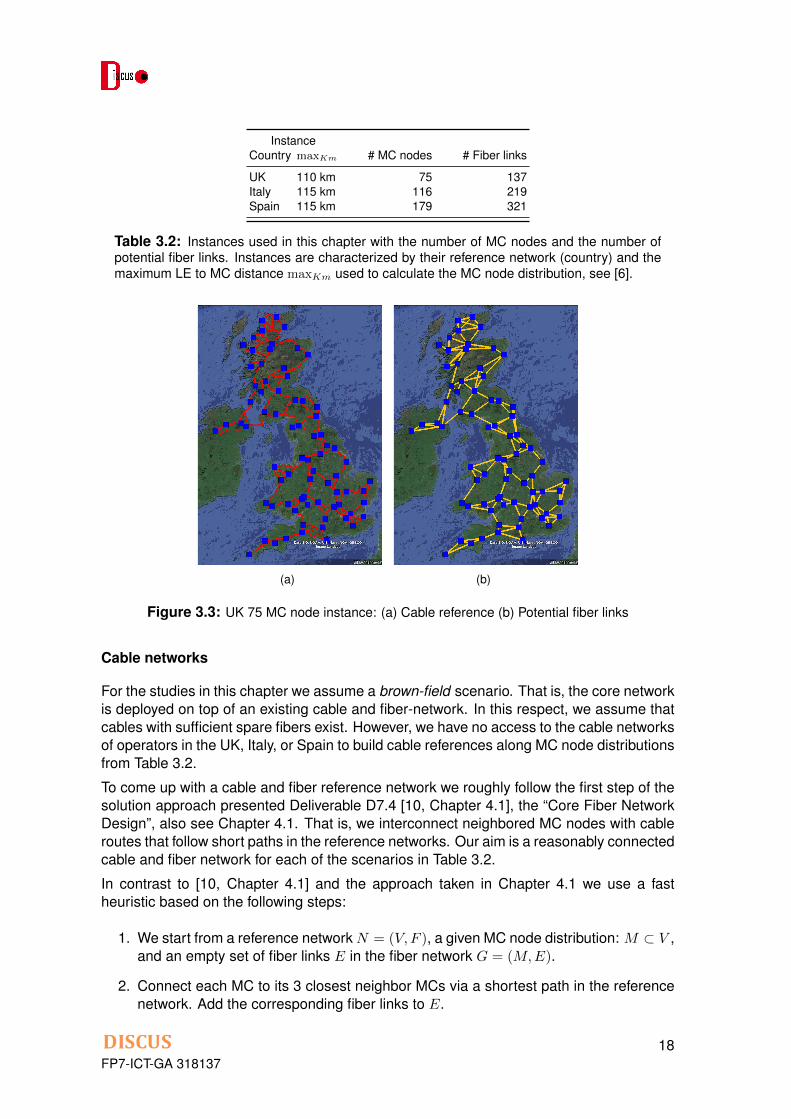
(a) (b)

Figure 3.3: UK 75 MC node instance: (a) Cable reference (b) Potential fiber links

Cable networks

For the studies in this chapter we assume a brown-field scenario. That is, the core networkis deployed on top of an existing cable and fiber-network. In this respect, we assume thatcables with sufficient spare fibers exist. However, we have no access to the cable networksof operators in the UK, Italy, or Spain to build cable references along MC node distributionsfrom Table 3.2.

To come up with a cable and fiber reference network we roughly follow the first step of thesolution approach presented Deliverable D7.4 [10, Chapter 4.1], the “Core Fiber NetworkDesign”, also see Chapter 4.1. That is, we interconnect neighbored MC nodes with cableroutes that follow short paths in the reference networks. Our aim is a reasonably connectedcable and fiber network for each of the scenarios in Table 3.2.

In contrast to [10, Chapter 4.1] and the approach taken in Chapter 4.1 we use a fastheuristic based on the following steps:

1. We start from a reference network N = (V, F ), a given MC node distribution: M ⇢ V ,and an empty set of fiber links E in the fiber network G = (M,E).

2. Connect each MC to its 3 closest neighbor MCs via a shortest path in the referencenetwork. Add the corresponding fiber links to E.

FP7-ICT-GA 31813718

3. Take the pair of MC nodes (m1

,m2

) with the largest shortest path distancelG(m1

,m2

) in G. If G is not yet connected, then lG(m1

,m2

) is infinite.

4. Let lN (m1

,m2

) be the shortest path distance in the original reference network N .

5. If lG(m1

,m2

) 2 · lN (m1

,m2

), then terminate.

6. Add the fiber link with length lN (m1

,m2

) to E. Go to step 4.

(a) (b)

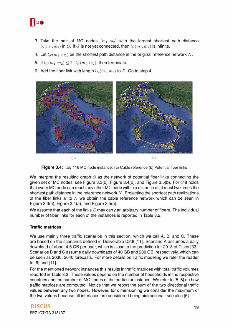
Figure 3.4: Italy 116 MC node instance: (a) Cable reference (b) Potential fiber links

We interpret the resulting graph G as the network of potential fiber links connecting thegiven set of MC nodes, see Figure 3.3(b), Figure 3.4(b), and Figure 3.5(b). For G it holdsthat every MC node can reach any other MC node within a distance of at most two times theshortest path distance in the reference network N . Projecting the shortest path realizationsof the fiber links E to N we obtain the cable reference network which can be seen inFigure 3.3(a), Figure 3.4(a), and Figure 3.5(a).We assume that each of the links E may carry an arbitrary number of fibers. The individualnumber of fiber links for each of the instances is reported in Table 3.2.

Traffic matrices

We use mainly three traffic scenarios in this section, which we call A, B, and C. Theseare based on the scenarios defined in Deliverable D2.8 [11]. Scenario A assumes a dailydownload of about 4.5 GB per user, which is close to the prediction for 2018 of Cisco [33].Scenarios B and C assume daily downloads of 40 GB and 280 GB, respectively, which canbe seen as 2030, 2040 forecasts. For more details on traffic modeling we refer the readerto [6] and [11].For the mentioned network instances this results in traffic matrices with total traffic volumesreported in Table 3.3. These values depend on the number of households in the respectivecountries and the number of MC nodes of the particular instance. We refer to [5, 6] on howtraffic matrices are computed. Notice that we report the sum of the two directional trafficvalues between any two nodes. However, for dimensioning we consider the maximum ofthe two values because all interfaces are considered being bidirectional, see also [6].

FP7-ICT-GA 31813719

(a)

(b)

Figure 3.5: Spain 179 MC node instance: (a) Cable reference (b) Potential fiber links

3.4 Solution methodology

There are several exact and heuristic approaches to tackle multi-layer network design, seefor instance [26, 59, 60, 64–66, 73]. The most common approach used in practice is prob-ably based on a bottom-up approach and decomposing the layer coupling. Starting fromthe highest network layer, each layer is dimensioned individually. Each layer dimensioningintroduces the input in terms of demands for the capacity dimensioning of the next layerin the stack. In terms of the introduced DISCUS layers, this means first providing a virtualtopology with capacitated links that is able to handle the given traffic matrix (ignoring thephysical topology), and, only in a second step, routing the virtual capacities (40G, 100G,400G channels) in the fiber network, while minimizing the fiber cost.

This approach, however, might yield to sub-optimal solutions, and may cause infeasibilities.In fact, by decomposition it is not guaranteed to find a solution even if there are many,see [72]. Moreover, decomposition ignores the fact that failures may occur in the lowestnetwork layers (in the cable or duct layer) but affect paths and services across all layers.

Starting from a given set of MC nodes M , a corresponding fiber network G = (M,E) asintroduced above, and a set of service links S ✓M ⇥M with demand values ds > 0, s 2 S

FP7-ICT-GA 31813720

Instance Traffic in TbpsCountry maxKm Demand scenario Reflected Core

UK 110 km A 178 221UK 110 km B 378 956UK 110 km C 1,373 6,014

Italy 115 km A 152 194Italy 115 km B 323 833Italy 115 km C 1,174 5,204

Spain 115 km A 253 321Spain 115 km B 536 1,404Spain 115 km C 1,944 8,736

Table 3.3: Total traffic volumes for the different network and demand scenarios. We state thetotal reflected traffic (traffic with source and target below the MC node not entering the core)and total core traffic.

(the traffic matrix), we will follow an integrated approach that tries to dimension the virtualtopology and physical topology simultaneously while minimizing the installation cost.

Following the terminology from [72] and we use a path-flow over path-flow model (withexplicit light-paths [64, 65] or disaggregated flow [72]). That is, in both layers, the virtualchannel layer, and the physical fiber layer we work with explicit set of paths. We only let theoptimization model decide which of the paths to chose. This approach has the flexibilityto work with different sets of preselected paths, easily integrating additional constraints onthe path realizations such as distance or topology restrictions, see Section 3.2. Of course,since we do not work with column generation, we can speak of optimality only with respectto the chosen set of paths.

Starting from the topology G = (M,E) of all potential fiber links we consider a preselectionof paths L in this topology. Each of these paths can be seen as the realization of a virtuallink, a potential channel connection. All preselected potential virtual links connecting theMC nodes form a virtual topology H = (M,L), see Figure 3.1.

Given the set of signals T , we denote by T` the subset of signals that can be used on theoptical channel link ` 2 L, that is, the length of the realization of ` does not exceed thesignal reach. Clearly, we may exclude from L all virtual links ` with T` = ;.In case of fixed-grid T contains 6 signal types: 40G, 100G, 400G, each either with orwithout the use of regenerators leading to a maximum signal reach of 5,000 kilometers.Similarly in case of flex-grid we have 12 different signal types, depending on the reach, thebitrate, the required bandwidth slots, and the use of regenerators, see Table 2.2.

We further denote by P all (virtual) paths in the virtual network H = (M,L). All pathscorresponding to a particular service s are denoted by Ps, that is, Ps contains all virtualpaths that can be used to realize the service link. Recall that within the strict optical islandconcept, any path in P should have not more than one hop, see 3.2.

We introduce the following three types of variables: Binary variable fp will indicate whethervirtual path p 2 P is used or not. Integer variables yt` counts how many optical channelswith signal type t 2 T are active on the virtual link ` 2 L. Eventually, integrals xe count howmany fibers are used on the fiber link e.

Given these variables the following model (TL) optimizes virtual and physical topologysimultaneously:

FP7-ICT-GA 31813721

(TL) minX

`2L

X

t2T`

tyt` +X

e2Eexe (3.1)

X

p2Ps

fp = 1, 8s 2 S, (3.2)

X

s2S

X

p2Ps

dsfp �X

t2T`

ctyt` 0, 8` 2 L, (3.3)

X

`2L:e2`

X

t2T`

rtyt` �Bxe 0, 8e 2 E (3.4)

fp 2 {0, 1} 8p 2 P, s 2 S

yt`, xe 2 Z+

8` 2 L, t 2 T`, e 2 E

Constraints (3.2) guarantee that exactly one path is chosen for each service. In an opticalisland this path is a direct virtual link between the two MC nodes. The inequality system(3.3) ensures that enough optical channels are used on a virtual link to carry the (packet)flow (in Gbps) of all paths using the link. The term ds denotes the traffic of the servicewhile ct is the bitrate capacity of the channel (40G,100G, or 400G). Similarly, system (3.4)ensures enough fibers on all fiber links. In these inequalities, the term rt refers to thenumber of bandwidth slots consumed by signal type t and B is the number of slots providedby a fiber (88 or 120). Notice that we ignore wavelength assignment in this model.

Objective (3.1) minimizes the cost of all required resources. The term t denotes thecost of an optical channel of type t 2 T . It includes the cost of two transponders and, ifnecessary, the cost of a regenerator. The term e denotes the cost of a fiber. In this casewe include the cost for WDM terminals on both sides, the cost for amplification (OLA) andthe cost for DGE, see 2.2.

3.4.1 A first step towards resiliency

Model (TL) is very flexible if used with different physical path sets L and virtual path setsP. However, it ignores resiliency in the sense that a failing fiber may cause services to fail.Resiliency within DISCUS is an end-to-end concept that already includes the dual homingfrom LE to MC sites. It clearly, has to be tested from an end-to-end perspective, see alsoChapter 4-6. In this chapter, we are not claiming to get solutions that are resilient down tothe level of cables and streets. We show how, in principle, a certain level of survivabilitycan be guaranteed across multiple layers. However, we go down to the fiber layer only(ignoring that two different fibers may follow the same street or duct system) and we donot introduce a hard resiliency constraint. Chapter 4 shows how solutions coming fromour optimizations can be improved such as to increase resiliency even down to the level ofstreets.

To introduce a certain level of resiliency we will use the following routing principle:

1. We route the traffic of each service on two different virtual paths p1

, p2

.

2. We verify that for any two virtual links `1

, `2

with `1

2 p1

and `2

2 p2

, the two physicalfiber realizations of `

1

and `2

do not use a common fiber link.

FP7-ICT-GA 31813722

This guarantees that any single fiber failure in the core does not lead to service interrup-tions as there is always a second open path with enough capacity between the end-nodesof the service. Notice that this ensures survivability on the fiber layer only. It does notguarantee resiliency on the cable or street level, see Figure 3.6. That is, we implicitly as-sume that two fibers having a cable/street link in common but take a different path in thecable/street topology are separated on the common link (in different cables, on differentsides of the street), also see Chapter 4.

(a) (b)

Figure 3.6: Zoom into the fiber (yellow) and cable (red) topologies of the (a) UK and (b) Italy.We can see that disjointedness on the fiber level does not mean disjointedness on the cablelevel. We also see one MC in both cases that has only one possible fiber connection to thenetwork.

Moreover, it turns out that for some instances caused by non-sufficient connectivity in thereference network not all MC nodes are connected to the fiber network by two disjointcore fiber routes, see Figure 3.6. At this point we could simply introduce additional linksto the fiber layer as these would probably exist in practice. Alternatively, we could removethese MCs from the distribution. However, this might introduce infeasibilities w.r.t the LE-MC connections. We decided to follow a third approach. We relax requirement 2. above,introduce a slack variable, and put into the objective function. That is, instead of a hardconstraint 2. we introduce a soft constraint, while minimizing its violation.The resulting overall survivability enhanced model (TLS) is as follows:

(TLS) minX

`2L

X

t2T`

tyt` +X

e2Eexe+

X

s2Szs (3.5)

X

p2Ps

fp = 2, 8s 2 S, (3.6)

X

s2S

X

p2Ps

dsfp �X

t2T`

ctyt` 0, 8` 2 L,

X

`2L:e2`

X

t2T`

rtyt` �Bxe 0, 8e 2 E

X

p2Ps:e2pfp 1 + zs, 8s 2 S, e 2 E (3.7)

fp, zs 2 {0, 1} 8p 2 P, s 2 S (3.8)yt`, xe 2 Z

+

8` 2 L, t 2 T`, e 2 E (3.9)

FP7-ICT-GA 31813723

Notice that we have marked changes to model (TL) in blue. Constraints (3.2) have changedto (3.6) requiring two virtual paths per service instead of only one. Constraints (3.7) arethe conflict constraints. They forbid paths of the same service to use the same fiber linksunless binary slack variable zs is switched on. In this case at most two paths may usethe same fiber link. However, the number of such situations is minimized in the new ob-jective (3.5), where the term

Ps2S zs counts how many services do violate the resiliency

requirement on at least one fiber link.

3.4.2 Path generation

Before solving models (TL) or (TLS) we have to generate reasonable sets of paths L inthe fiber graph G = (M,E) and given the resulting virtual graph H = (M,L) we have toprovide a set of virtual paths P. Clearly, all these paths should be short but they shouldalso be designed to share common sources (fibers, optical channels). Moreover, in orderto fulfill the resiliency constraint (3.5) (with zs = 0 if possible) we need paths P that aredisjoint when mapped to the fiber graph G.

Recall that in case of the pure optical island concept the set P is in fact identical to L. moreprecisely each path in P consists of exactly one link in L. However, we will compare moregeneral architectures (with optical islands) such that we allow P to contain paths with innernodes, allowing to groom traffic at intermediate MCs.

Our path generation process consists of three main steps:

• Path computation

• Path expansion

• Path filtering

Path computation

We may distinguish path computation in the physical and the virtual layer.

In the physical layer, we mainly use the Dijkstra’s algorithm [39] to compute short pathsand the Suurballe’s algorithm [57, 90] to compute short and disjoint paths. In additionwe heuristically determine disjoint paths by iteratively computing shortest paths with linkweights that forbid the links of the previous iteration. We call these paths alternative short-est paths.

In the default settings, for any pair of MC nodes, we compute a shortest path, 3 disjointpaths using Suurballe’s algorithm, and 2 alternative shortest paths. All these paths createthe set of virtual links L, a set of potentially 6 · |M |(|M |�1) elements. Recall that we do notallow virtual links that are too long in the sense that there is no signal type with sufficientreach.

In the now created potential virtual layer H = (M,L) we first create all single-hop paths,that is, all paths that use one of the links in L. We further generate all short two-hop pathsbetween any pair of MC nodes. We might, however limit the allowed intermediate MCs (thegrooming locations), see below. Then again we compute all shortest paths in H. Theseare not necessarily single hop paths as there might be pairs of MC nodes that have nodirect virtual link (because of the mentioned signal reach restrictions).

FP7-ICT-GA 31813724

We further compute shortest virtual paths with a weight function that is based on the trafficvolume. In this case a virtual link is defined short if there is large demand between its MCend-nodes. Intuitively, we want to create virtual paths that follow the traffic pattern and uselinks/nodes with large demand. All these paths enter the initial set PWe create many more possible virtual paths by Path expansion:

Path expansion

(a) (b)

(c) (d)

Figure 3.7: Path expansion. (a) Original path; (b)-(d) All possible path expansions. Fiberlinks are in yellow, virtual links in black.

From each path in p 2 P we create a series of paths by following the same physical pathbut allowing for different intermediate grooming MCs. This can be done by first mappingthe path p to the physical layer G in order to see which MC nodes Mp are visited by p.More precisely, the set Mp contains all inner nodes of p (all grooming locations) and allnodes that are inner nodes of the virtual links contained in p. The latter nodes are opticallybypassed by p.

In a second step, we consider all subsets M 0p of Mp and create new paths p0 by using all

MCs in M 0p as inner nodes following the same physical path, see Figure 3.7. We add all

paths p0 corresponding to subsets M 0p to P. Clearly, all paths p0 use the same fiber links a

p, that is, have the same physical representation but they use different virtual links, whichallows for different intermediate grooming. Notice that the path expansion operation mightcreate new virtual links that where not generated by the physical path computation above.These are added to L.

Path expansion can be an expensive operation both in terms of CPU-time and memoryusage since subsets are generated. To control the necessary computing resources we tryto include path filtering mechanisms already in the path expansion.

Path filtering

After path computation and path expansion we use several filtering techniques to reducethe size of the sets P and L and in order to implement different restrictions on the allowedpath realizations. The main filtering criteria are:

• The number of virtual hops k >= 1. Paths p 2 P only pass this filter if the number ofhops does not exceed k.

• The set of allowed grooming locations Mgroom ✓M . Paths p 2 P pass the filtering ifthey are sing-hop paths or if they contain inner nodes from Mgroom ✓M only.

FP7-ICT-GA 31813725

• We may further force grooming for selected (e.g. small) MC locations M small ⇢ M .If m 2 M small then any path in p with m as end-node has to contain a location fromMgroom. In particular, if both end-nodes are from M small path p needs an intermedi-ate node from Mgroom. We either set M small := ; or M small := M\Mgroom.

With the first filter, by setting k := 1, we force optical island topologies. By combining thelast two criteria we may force two-tier topologies, that is, topologies where the traffic frompreselected (smaller) nodes needs to get aggregated at preselected inner core nodes.

Clearly, all of the filtering criteria can partially be incorporated already in the path compu-tation and expansion.

Instance Cost in Mio eCountry maxKm Traffic Scenario Channel Fiber Switch Total

uk 110 km A OPT 331 51 140 522uk 110 km A GROOM 340 46 154 540uk 110 km A ISLAND 475 93 148 716

italy 115 km A OPT 494 107 189 790italy 115 km A GROOM 526 111 202 839italy 115 km A ISLAND 769 230 226 1224

spain 115 km A OPT 833 182 311 1325spain 115 km A GROOM 871 190 326 1387spain 115 km A ISLAND 1784 504 519 2807

Table 3.4: Cost of the core network for different architectures and networks. Trafficscenario A. Channel cost includes cost for transponders (fixed grid), regenerators, andtransceivers. Fiber cost means cost for WDM terminals, OLAs, and DGEs. Switch cost iscost for MPLS-TP switches, Polatis switches as well as for line-cards.

3.5 Computations

In this section, we use the presented data and methodology to dimension the core ofthe DISCUS architecture. In the first part, we evaluate the cost of optical islands for thenetwork instances from Table 3.2 and compare this cost with two alternative architectures.In the second part we will study how the different architectures scale with increasing trafficvolumes. In particular, we will try to understand under which conditions optical islands arecost-effective compared to architectures that allow for traffic grooming in the core or use asecond level of traffic aggregation.

To solve the models (TL) and (TLS) we use the solver CPLEX 12.6 multi-threaded with upto 6 cores and up to 50 GB RAM on a machine with 10 CPUs (2.8 Ghz). We set the timelimit to 10,000 seconds and the emphasis of the solver to finding feasible solutions.

Table 3.4 summarizes the results of our first experiment using the traffic scenario A (2018)and model (TLS). We distinguish three different runs of the optimization routine with differ-ent settings w.r.t the envisaged architecture:

• ISLAND: We force an optical island architecture by setting k := 1 in the path filteringas explained above. Regenerators are used if necessary.

FP7-ICT-GA 31813726

• GROOM: We force a two-tier type architecture by setting Mgroom to the 10 biggestMC locations. All traffic has to be groomed at these nodes (M small := M\Mgroom).The maximum number of virtual hops is restricted to k := 3.

• OPT: We still set Mgroom to the 10 biggest locations. Grooming is allowed only atthese nodes. However, we do not force grooming (M small := ;) as in GROOM. Themaximum number of virtual hops is restricted to k := 3.

Notice that the solution space corresponding to the third setting includes the solutionspaces of the first two.

(a) (b)

Figure 3.8: Virtual layer of (a) ISLAND: Full mesh optical island solution (b) GROOM: Solutionwith grooming at the 10 biggest MCs (in red); all optical channels start or end at one of these10 nodes.

Table 3.4 shows the cost in Mio e of the different solutions. We state the cost occurringin the core only. That is, for dimensioning the line-cards and switches, we ignore anyport needed in the access and we ignore traffic that is reflected at the MC node. It canbe seen that a two-tier architecture (GROOM) outperforms the optical island (ISLAND) interms of cost using traffic scenario A. The cost can be decreased even further if we relaxthe requirement to groom at one of the 10 big locations and allow for direct links betweensome of the smaller locations. That is, a mixture of the optical island and the two-tierconcept gives the cheapest network. However, the difference between the best cost andthe cost for the optical island decreases with a decreasing number of MC nodes. We save1,482 Mio e (52.8%) for Spain 434 Mio e (35.5%) for Italy, but only 194 Mio e (27.1%) forthe UK.

We note that all optical island solutions can be considered being optimal (optimality gapsbelow 1%). However, in particular the solutions for Italy and Spain and scenarios OPTand GROOM have potential to be improved (optimality gaps larger than 20%). This meansthat the mentioned differences might in fact be even larger. Moreover, even scenario OPTintroduces restrictions on the allowed virtual topologies. Further relaxing these restrictions(allowing for multi-hop paths with k > 3, allowing for more grooming locations than 10,etc.) might further decrease the cost for OPT.

This seems to be bad news for the optical island concept unless we have small countrieswith a possibly small number of MC nodes as in the case of the UK. However, the picture

FP7-ICT-GA 31813727

Instance Cost in Mio eCountry maxKm Traffic Scenario Channel Fiber Switch Total

uk 110 km 0.01·A opt 19 16 23 58uk 110 km 0.01·A groom 19 16 23 58uk 110 km 0.01·A island 284 74 77 435




uk 110 km A opt 331 51 140 522uk 110 km A groom 340 46 154 540uk 110 km A island 475 93 148 716




uk 110 km B opt 1348 172 508 2028uk 110 km B groom 1510 143 680 2332uk 110 km B island 1445 199 503 2146


uk 110 km C opt 8748 959 3217 12923uk 110 km C groom 10328 860 4655 15843uk 110 km C island 8890 1022 3215 13128

Table 3.5: Cost of the core network for the UK network with 75 MC nodes and different trafficscenarios. We used the traffic scenarios A, B, and C and also scaled scenario A with factorsfrom {0.01, 0.1, 0.3, 0.5, 2.0, 3.0, 4.0, 8.0}.

changes completely if we change the size of the traffic matrix focusing on the scalability ofthe architectures in terms of future traffic.

In Table 3.5 we report on the same computations (UK network) but with different(scaled) traffic matrices. We use matrix A as in Table 3.4 scaled with a factor from{0.01, 0.1, 0.3, 0.5, 1.0, 2.0, 3.0, 4.0, 5.0} and matrices B, C. It can be seen that for smallertraffic volumes an architecture based on grooming traffic clearly outperforms any opticalisland concept. With traffic matrix 0.01 · A the cost of an optical island is 7.5 times thecost for a two-tier architecture. In fact with very small traffic, the cost of an optical island isindependent of the traffic as we have to open one channel for each pair of nodes anyway.In case of the UK the total optical island cost is relatively constant between 435 Mio e and477 Mio e although the traffic increases by a factor of 300.

However with larger traffic volumes the advantage of grooming decreases and at somepoint optical islands outperform architectures which force to groom. Already a matrix ofsize 3 times A (around 700 Tbps total core traffic) makes the optical island cheaper than

FP7-ICT-GA 31813728

0

500

1,000

1,500

2,000

2,500

3,000

3,500

0 500 1,000 1,500 2,000

Netw

ork

Cost

in M

io E

UR

Traffic in Tbps

OptIslandGroom

Figure 3.9: Cost of different architectures as a function of the traffic volume, UK network with75 MC nodes, LEs connected with a maximum distance of 110 km.

the grooming architecture (1435 Mio e versus 1483 Mio e ). Figure 3.9 shows the costcurves as a function of the traffic and clearly visualizes the threshold of around 700 Tbps.

Of course, a mixture of both concepts (grooming to fill up the channels and optical islandsfor scalability), that is scenario OPT, gives the best results as it allows to groom trafficwhen necessary, that is, for very small MC nodes and for traffic values that are not exactmultiples of 40, 100, 400 Gbps. It should also be noticed that for higher volumes of trafficthe value found for OPT converges to that for ISLAND, clearly indicating that the use ofoptical islands tends to be the solution of choice for increasing traffic volumes.

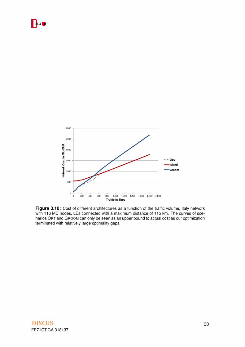
We close with Figure 3.10, which presents similar results for the Italian network. We cansee a similar behavior of the cost curves. However, the cost values for GROOM (and alsoOPT) are not as resilient as for the UK because our optimization terminated with relativelylarge optimality gaps ( > 20%). They can only be seen as an upper bound to the actualcost such that the actual cost function for GROOM (and OPT) might (!) be below the one inFigure 3.10.

3.6 Conclusion

In this chapter, we showed how to solve multi-layer core network design problems in orderto assess the impact of the DISCUS optical island concept. For different European coun-tries and different metro-core nodes locations, we solve an integrated planning problemincluding the dimensioning of the virtual channel layer and the physical cable/fiber layer.

Using our methodology we optimized different types of core networks based on differentarchitecture assumptions. We were able to show that optical islands outperform architec-tures based on aggregating (grooming) traffic towards an inner core once the traffic volumeexceeds a certain threshold depending on the cost model, the number of metro-core nodesand the available channel capacities (40G, 100G, 400G).

For the UK this threshold is around 700 Tbps total core traffic using the cost model fromChapter 2 and the smallest channel bitrate being 40 Gbps.

FP7-ICT-GA 31813729

0

1,000

2,000

3,000

4,000

5,000

6,000

0 200 400 600 800 1,000 1,200 1,400 1,600 1,800 2,000

Netw

ork

Cost

in M

io E

UR

Traffic in Tbps

OptIslandGroom

Figure 3.10: Cost of different architectures as a function of the traffic volume, Italy networkwith 116 MC nodes, LEs connected with a maximum distance of 115 km. The curves of sce-narios OPT and GROOM can only be seen as an upper bound to actual cost as our optimizationterminated with relatively large optimality gaps.

FP7-ICT-GA 31813730

Chapter 4

Resilient core network planning

Ensuring network survivability in the presence of failures is a crucial prerequisite in provid-ing highly reliable network operation with low outage times. Optical core networks are vul-nerable to a wide set of failures, ranging from individual component faults due to physicaldamage (e.g., link cuts) or fatigue, over disaster-like events affecting entire M/C nodes orwider geographical areas, to intentional malicious activities aimed at disrupting the service.This chapter focuses on ways of providing survivability in the network planning phase byconsidering single link- and node-component failures as well as deliberate physical-layerattacks targeting service disruption.

Section 4.1 addresses the requirement for survivability from link and/or node failures in thenetwork design phase. Link cuts due to, e.g., construction equipment ploughing throughthe ducts are the most common cause of component failures. Failures of entire nodes canbe seen as disasterous events disconnecting thousands of users. To adress this issuenew, 3-step network design approach is proposed which increases the number of DISCUSreference network node pairs for which physically disjoint paths can be found, such thatthe total distance between all node pairs is minimized and the path lengths do not exceedthe optical signal reach.

Section 4.2 focuses on individual node component failures and investigates means of in-creasing network reliability through the deployment of synthetic programmable ROADMsimplemented by Architecture on Demand (AoD). Such nodes provide unprecedented levelsof flexibility and are capable of so-called self healing, allowing for node components fail-ures to be healed at the node level without triggering network-level recovery mechanisms.A connection routing approach is proposed to enhance the self-healing functionality andreduce the number of failures which require recovery at the network level.

Section 4.3 studies vulnerability of transparent optical networks to deliberate physical-layerattacks aimed at service disruption. Since such attacks do not occur often, but can causemajor wide-area damage in case they do appear, high resource-efficiency is particularlydesirable in resiliency schemes which consider attacks. Therefore, consideration of attacksneeds to be incorporated into the network planning procedures as an additional damage-reduction criterion while maintaining standard optimization objectives typically aimed atminimizing resource usage and cost. To this end, an attack-aware approach for dedicatedpath protection is developed to reduce the number of connection which remain unprotectedin the presence of an attack while using the same number of wavelengths as standard,resource-minimizing protection approach.

Section 4.4 focuses on advantages of dual-homed networks in providing resource-efficientsurvivability from core link failures. Dual homing has the potential to improve resource-usage efficiency by allowing greater flexibility in the selection of backup paths. A dedicatedpath protection approach is proposed to utilize this property and satisfy the availabilityrequirements of connection requests at a lower resource consumption.

FP7-ICT-GA 31813731

4.1 Resilient core network design

Survivability to device failures is a fundamental requirement in core networks since a sin-gle failure in the network could interrupt on-line services in social and business life [71].Finding a minimum distance resilient optical core network is an intractable problem sinceit includes the constrained shortest path problem as special case [99]. Even the networkdesign is fixed, for general undirected graphs, finding node-disjoint paths is NP-complete[31].

The problem considered in this section is finding the minimum distance design (MDD)networks for both abstract and street levels where the disjointness is maximised. Moreformally, a set of trails from given street network with minimal total length are selected sothat there exists two bounded paths between each pair of metro core nodes with maximaldisjointness. In addition to the theoretical computational complexity of the problem, dueto the size of the nation-wide street networks where nodes and edges refer road junctionsand trails, there is also a scalability problem in practice. Therefore, in this section, wedecompose the problem into three steps.

Developed 3-step approach starts with abstraction process which reduces the street net-work with road junctions and road links (i.e., trails) to an abstract network where nodesand edges refer to the metro-core nodes and the links between them. After that, in thesecond step of the algorithm, a mixed integer programming (MIP) decomposition basedalgorithm is used to find the minimum distance bounded node disjoint resilient abstractnetwork. Although it is possible to find high level of node disjointness after the second stepin the abstract level, the actual disjointness which is computed after projecting/mapping theabstract solution into the street network is most likely less than the desired level. Hence,in the last step of the algorithm, we propose a greedy method to improve the disjointnessof the paths between metro-core nodes. A flowchart of the 3-step algorithm is presentedin the following and details of each step are discussed in the next sections.

STEP 1 Abstraction: Find the abstract network.

Street network input data: Junctions, Local exchanges, Metro-core nodes, trails, traffic between metro-core nodes.

STEP 2 Optimisation: Find the minimum distance design network in the abstract level that maximises node disjoint pair of nodes and minimises sharing of nodes and links.

STEP 3 Projection and improvement: Map the abstract network solution into the street network solution and improve the number of node disjoint pairs, shared nodes and the length of the links shared.

Figure 4.1: Flowchart of the 3-step algorithm for resilient core network design

FP7-ICT-GA 31813732

4.1.1 STEP 1: Abstraction

In this first step, we reduce the street network with road junctions and trails into an ab-stract network where metro-core nodes are nodes and the possible links between themare edges of the graph. Details of the abstraction procedure is given in the following.

• Let Gr = hV r, Eri be the graph corresponding to the street network.

• Let Ga = hV a, Eai be the graph corresponding to the abstract network. Here V a

correspond to the set of MC-nodes.

• SP (i, j, Gr � B) is the shortest path between metro core nodes i and j in Gr whichexcludes all other metro-core nodes to guarantee that if it exists, it does not rely onany other metro-node. If such a path does not exist, initially it is known that there isno node-disjoint path between the corresponding metro-nodes.

Based on these definitions, the abstraction procedure is given in the following which isexecuted for every pair of metro-core nodes and computes the length of the abstract linkbetween these pairs as the length of the shortest path in the street network.

for all {hi, ji|i 2 N ^ j 2 N ^ i 6= j} doB N \ {i, j}|e| = |SP (i, j, Gr �B)|

Size of the resulting abstract UK, Italy and Spain networks are summarized in Table 4.1.Note that sizes of the initial abstract and street networks refer to the sum of the all possiblelinks.Due to overlapped trails in different abstract network links, size of the sreet network ismuch smaller than the abstract network. Assume that it is required to construct a shortestpath between metro core nodes 31 and 95 in the abstract level. And furthermore, firsttwo links in the shortest path are the abstract links between metro core nodes (31-32) and(32-84). When we compute the projection of abstract link (31-32) in the street network, weobserve that the last two trails of this abstract link are (in order of occurrence in the path)trail number 29237 and 15186. Similarly, when we compute the projection of abstract link(32-84) in the reference network, first two trails are (in the order of the occurrence), trailnumbers 15186 and 29237. In other words, the same trails are used in the path between31-32 and 32-84 for connecting metro core node 32 to others. Since the length of theabstract links are immutable, we are incurring the length of these two trails twice in theabstract level solution. However, when we compute the projection in the street networklevel, we’re omitting the repeated occurrences of the same trails. Hence, the total length ofthe shortest path between 31 and 95 is in the abstract network is longer than its projectionin the street network. Therefore, the total length of the links (i.e., size of the network) inthe abstract level is more than its mapping in the street level.In addition, an initial analysis on these network topologies also show that some pair ofnodes don’t have node disjoint paths. There are 8 pair of metro-core nodes related withSardinia, Sicily and Elba islands for Italy topology which have no node-disjoint paths inthe street network withing the signal reach. Similarly, in UK reference network, metrocore node MC—scotland—Ex—4587 requires a mandatory link to metro-core node MC—scotland—Ex—4754 to connect to the nationwide UK network. Therefore, any k pathsoriginating from or terminating in MC—scotland—Ex—4587 are not node disjoint.

FP7-ICT-GA 31813733

UK Italy SpainNumber of metro core nodes (N ) 75 116 179Number of nodes in the street network, road junctions, (V r ) 15608 23689 18819Number of edges in thestreet network, trails, (E r ) 23027 32702 26480Number of nodes in the abstract network (V a ) 75 116 179Number of edges in theabstract network (E a ) 2775 6670 15931Number of not disjoint pair of metro-nodes in the street network 74 8 0Number of not disjoint pair of metro-nodes in the abstract network network 74 8 0Initial abstract network size, STEP 1 (km) 1279529 4835343 8765621Initial street network size, STEP 1 (km) 22880 23155 37606

Table 4.1: Size of the Street and the Initial Abstract Networks

4.1.2 STEP 2: Designing Minimum Distance Node Disjoint Abstract Network

Once we create the abstract graph which consists of metro-core nodes, N , and all possiblelinks between them, L, in this step, we select a subset of these links to minimise thetotal length and to ensure maximal node disjointness between any pair of nodes. Formaldefinition of the problem solved in this step is given in the following :

Definition 1 (All-Pairs k Node-Disjoint Length-Bounded Paths Problem). Given a graphhN,Li where N is a set of nodes N and L is a set of links, the All-Pairs k Node-DisjointLength-Bounded Paths Problem (AkNLPP) is to determine k � 2 bounded paths betweeneach pair of nodes {i, j} ✓ N . The objective is to first minimise the number of pairs ofnodes whose k paths are not node-disjoint, then minimise the sum of the number of nodesshared between two or more selected paths associated with the pairs of nodes which arenot node-disjoint, then minimise the sum of the lengths of the links shared between two ormore selected path of pair of nodes that are not node-disjoint, then minimise the weightedsum of the selected links used by all the selected paths and finally minimise the weightedsum of the lengths of all the paths.

There are five cases for a given pair of MC-nodes that can be observed while solvingresilient network design problem:

1. There exists k disjoint paths and length of each one of them is within the maximumsignal reach.

2. k disjoint paths do not exist and the length of the shortest path is within maximumsignal reach.

3. k disjoint paths do not exist and the length of the shortest path is more than themaximum signal reach.

4. There exists k disjoint paths but the length of only some of them is within maximumsignal reach and the length of the others exceeds the reach.

FP7-ICT-GA 31813734

5. There exists k disjoint paths but the length of each one of them exceeds the maxi-mum signal reach.

However, even classifying a given pair of nodes into one of these options is also anNP-hard problem. Hence, there is a need for effective heuristic methods for solving theAkNLPP problem. Beforehand, in the following, we provide a novel model formulation tomathematically define the problem with the following multi-objectives in the order of pref-erences

1. Maximise the number of pairs with 100% node disjoint paths which are classified ascase 1.

2. Maximise partial disjointness which means minimising the number of nodes and thelength of the links shared between paths if 100% node disjoint paths are not possiblewhich are classified in cases 2– 5.

3. Minimise the distance based size of the network.

4. Minimise the length of the paths due to minimise transponder costs.

where the following constraints must be ensured

1. Find k paths for each pair of metro-nodes ⌧ 2 †.

2. Length of each of k paths must be less than the maximum signal reach.

The reason why we distinguish between the number of pairs with fully disjoint paths (i.e.,no shared nodes between paths, 100% disjointness) and the partial disjointness (i.e., atleast one node and/or link is common between paths) is due to model five special casesdescribed above. In other words, any method that aims to solve ”All-Pairs k Node-DisjointLength-Bounded Paths Problem” must search for finding fully k disjoint paths for pair ofmetro-nodes and for ones that it is not possible, must find k paths that shares minimumnumber of nodes and length of links common. Finally, the same level of disjointness mustbe ensured with a network with minimum size in terms total length of the links and the min-imum sum of path lengths. In the following, we provide a general mathematical formulationto model ”All-Pairs k Node-Disjoint Length-Bounded Paths Problem”.

Sets and Indices

• i 2 N : the set of metro-core nodes,

• l 2 L : the set of all all possible links between metro-core nodes and is also denotedas {i, j}

• e, a 2 E: set of all directed edges between metro-core nodes. A link between metro-nodes i and j is undirected. If a physical link is installed between any pair of metro-core nodes, say i 2 N and j 2 N , then two edges hi, ji and hj, ii are defined becauseof bi-directional data transfer.

• ⌧ 2 † = {hi, ji|i 2 N ^ j 2 N ^ i 6= j} : the set of all directed pairs of metro-nodesbetween which connection requests can be made

FP7-ICT-GA 31813735

• k 2 K : index of node disjoint paths

Parameters

• cl: the cost of a link l 2 L end is equal to the length of the link.

• |e|: length of a directed edge e 2 E which is equal to the length of the correspondinglink.

• In(i) (Out(i)): all edges entering (leaving) node i 2 N .

• � : the maximum reach of any allowed optical signal, which is 2430km.

• s(⌧) (t(⌧)) : source and target nodes of pair ⌧ 2 † respectively.

• "⌧ : traffic between source and target nodes of pair ⌧ 2 †.

• ↵, �, � and ✓: big numbers that are used to model preference of objective functionssuch that ↵� � � � � ✓.

Variables

• w⌧ : a binary variable for each pair of metro nodes that is true if and only if any twoof the k paths share at least one node. In other words, this binary variable is true ifad only if all of k paths are not fully disjoint (i.e., partially disjoint).

• z⌧ i : a binary variable for each pair and node that is true if and only if node i 2 N isshared by at least two of k 2 K paths of pair ⌧ 2 †.

• yl : a binary variable for each link l 2 L which is true if and only if the link is includedin the resilient optical island.

• xk⌧e : a binary variable that is true if and only if edge e is used by path k of directedpair of nodes ⌧ 2 †.

• q⌧e : a binary variable that is true if and only if edge e is is shared by at least two ofk 2 K paths of pair ⌧ 2 †.

All-Pairs k Node-Disjoint Length-Bounded Paths Problem

min↵⇥X

⌧2†w⌧+�⇥

X

⌧2†

X

i2Nz⌧ i+�⇥

X

⌧2†

X

e2E|e|⇥q⌧e+✓⇥

X

l2Lcl⇥yl+

X

⌧2†"⌧⇥

X

e2E

X

k2K|e|⇥xk⌧e

(4.1)

8⌧2†8k2K :X

e2In(s(⌧))

xk⌧e = 0,X

e2Out(s(⌧))

xk⌧e = 1 (4.2)

8⌧2†8k2K :X

e2Out(t(⌧))

xk⌧e = 0,X

e2In(t(⌧))

xk⌧e = 1 (4.3)

8⌧2†8i2N\{s(⌧),t(⌧)}8k2K :X

e2In(i)

xk⌧e =X

e2Out(i)

xk⌧e (4.4)

FP7-ICT-GA 31813736

8⌧2†8k2K :X

e2E|e|⇥ xk⌧e � (4.5)

8⌧2†8l⌘{i,j}2L8e2{hi,ji[hj,ii}8k2K : yl � xk⌧e (4.6)

8⌧2†8i2N\{s(⌧),t(⌧)} :X

e2In(i),k2K

xk⌧e 1 + (|K|� 1)⇥ z⌧ i (4.7)

8⌧2† :X

i2Nz⌧ i |N |⇥ w⌧ (4.8)

8⌧2†8e,a2E|s(e)<t(e)^s(e)=t(a)^t(e)=s(a) :X

k2Kxk⌧e + xk⌧a 1 + (|K|� 1)⇥ q⌧e (4.9)

8⌧2†8i2N :X

e2E,k2K|s(e)=i^t(e)=i

xk⌧e � z⌧ i (4.10)

8⌧2†8e2E|s(e)<t(e) :X

k2k(xk⌧e +

X

a2E|s(a)=t(e)_t(a)=s(e)

xk⌧a) � q⌧e (4.11)

8⌧2† : w⌧ X

i2Nz⌧ i (4.12)

X

l2Lyl � |N | (4.13)

8⌧2† : w⌧ 2 {0, 1} (4.14)

8⌧2†8i2N : z⌧ i 2 {0, 1} (4.15)

8⌧2†8e2E : q⌧e 2 {0, 1} (4.16)

8⌧2†8e2E8k2K : xk⌧e 2 {0, 1} (4.17)

8l2L : yl 2 {0, 1} (4.18)

Objective function (4.1) minimises the weighted sum of the number of partially disjointpairs, total number of shared nodes, weighted sum of the lengths of the shared lengthsfor partial disjoint pairs, the total length of the links used and the total length of the pathsfor each pair of nodes that are weighted by the traffic between them. Note that we useweighted-sum method [79] to formulate this multi-criteria objective function (4.1).

Constraints (4.2) - (4.6) are used to model the network design part of the problem. Con-straints (4.2) and (4.3) ensure that for each pair of nodes, no route should reach the sourcenode or leave the target node and exactly one edge must leave (reach) from (to) the source

FP7-ICT-GA 31813737

(the target) node. Constraints (4.4) enforces that at each intermediate node of paths theincoming degree should be equal to the outgoing degree. The length of the route fromsource to target cannot exceed the threshold for each path of ⌧ 2 † with constraints (4.5).Constraints (4.6) guarantee that a link l between nodes i and j is selected if any corre-sponding directed edge between them is used by at least one of the k paths of any pair ofnodes.

Constraints (4.7) - 4.9 model node and link sharing. Constraints (4.7) label common inter-mediate nodes for each ⌧ 2 † if they are shared by at least two of k paths. Constraints (4.8)indicate that paths of pair of metro-node ⌧ 2 † are not node disjoint if at least one nodeis shared between two or more paths. Similarly, 4.9 label common links that are sharedbetween two or more paths of each ⌧ 2 †.Constraints (4.10) - (4.12) are formulated as valid inequalities which help to prune thesearch space. Constraints (4.10) bound the value of z variables for each pair and nodeand guarantee that the variable is equal to 1 if and only if that node is used in more thanone path of the corresponding pair of nodes. Similarly, Constraints (4.11) ensure that a linkis labeled as ”shared” for a pair of nodes if and only if the link is shared by at least two ofk paths of that pair. Constraints (4.12) give a valid upper-bound for node disjoint indicatorvariables for each pair of nodes ⌧ 2 † and ensure that w⌧ variable take value 1 if and only ifthere exist at most one common node shared by some of k paths of that pair. Total numberof selected link is at least equal to the number of nodes which is a valid inequality for theresilient optical network design problem and formulated as in (4.13).

The MIP model provided above is able to capture all properties of the problem and aims tosolve the problem at once with all pair of nodes. However, solving the model is intractableespecially for nation-wide networks where the number of pair of metro-core nodes might bemore than 10.000.Therefore, we develop a decomposition algorithm (Algorithm 1) whichsolves the optimisation model for only one pair of nodes at a time and updates the set ofused links iteratively.

Algorithm 1 also decomposes the complex objective function in equation 4.1 into two partsby using two different MIP models called in methods FINDCHEAPESTBOUNDEDFULLYN-ODEDISJOINTPATHS and FINDCHEAPESTBOUNDEDMAXIMALNODEDISJOINTPATHS. Fora given pair of metro core node ⌧ , Algorithm 1 first tries to find K node disjoint pathswhile minimising the distance based cost by calling the FINDCHEAPESTBOUNDEDFUL-LYNODEDISJOINTPATHS method. If the MIP model used in FINDCHEAPESTBOUNDEDFUL-LYNODEDISJOINTPATHS method can’t find K node disjoint paths, then FINDCHEAPEST-BOUNDEDFULLYNODEDISJOINTPATHS method is called and K paths with maximal dis-jointness are found. Details of these methods are given in Figures 4.2 and 4.3. Note thatconstraints 4.25 in Figure 4.2 are formulated to forbid direct links between the source andtarget nodes.

FP7-ICT-GA 31813738

Algorithm 1 BOUNDEDNODEDISJOINTNETWORK(†,N ,L,K)1: Sort † based on non-decreasing order of |SHORTESTPATH(⌧, L)|2: E {hi, ji [ hj, ii|{i, j} 2 L}3: 8⌧2† 8k2K 8e2E xk⌧e is a binary variable4: Lb ; , pathK⌧ ;5: while † 6= ; do6: Remove the first element ⌧ from the sorted set †7: xK⌧ FINDCHEAPESTBOUNDEDFULLYNODEDISJOINTPATHS(⌧ ,N ,L,Lb,K)8: if xK⌧ = ; then9: xK⌧ FINDCHEAPESTBOUNDEDMAXIMALNODEDISJOINTPATHS(⌧ ,N ,L,Lb,K)

10: pathK⌧ {e |xk⌧e = 1 ^ e 2 E}11: Lb {l ⌘ {i, j} |xk⌧e = 1 ^ e ⌘ hi, ji 2 E}12: return [Lb, pathK ]

min↵⇥X

l⌘{i,j}2L\Lb

X

e2{hi,ji[hj,ii}

X

k2Kcl · xk⌧e + "⌧ ⇥

X

e2E

X

k2K|e| · xk⌧e (4.19)

8k2K :X

e2In(s(⌧))

xk⌧e = 0,X

e2Out(s(⌧))

xk⌧e = 1 (4.20)

8k2K :X

e2Out(t(⌧))

xk⌧e = 0,X

e2In(t(⌧))

xk⌧e = 1 (4.21)

8i2N\{s(⌧),t(⌧)}8k2K :X

e2In(i)

xk⌧e =X

e2Out(i)

xk⌧e (4.22)

8k2K :X

e2E|e|⇥ xk⌧e � (4.23)

8i2N\{s(⌧),t(⌧)} :X

e2In(i),k2K

xk⌧e 1 (4.24)

X

e2In(i),k2K|s(e)=s(⌧)^t(e)=t(⌧)

xk⌧e 1 (4.25)

8e2E8k2K : xk⌧e 2 {0, 1} (4.26)

Figure 4.2: FINDCHEAPESTBOUNDEDFULLYNODEDISJOINTPATHS(⌧ ,N ,L,Lb,K): FIND KCHEAPEST BOUNDED NODE DISJOINT PATHS BETWEEN THE MC NODES OF ⌧

Size of the initial networks presented in STEP 1 are reduced as shown in 4.2 by usingAlgoritm 1 for K = 2. Note that MDD (Minimum Distance Design) is used to underline thesize of the network after minimum number and total length of the links are selected.

FP7-ICT-GA 31813739

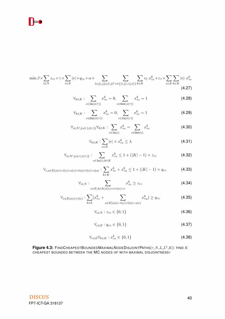
min�⇥X

i2Nz⌧ i+�⇥

X

e2E|e|⇥q⌧e+↵⇥

X

l⌘{i,j}2L\Lb

X

e2{hi,ji[hj,ii}

X

k2Kcl ·xk⌧e+"⌧⇥

X

e2E

X

k2K|e|·xk⌧e

(4.27)

8k2K :X

e2In(s(⌧))

xk⌧e = 0,X

e2Out(s(⌧))

xk⌧e = 1 (4.28)

8k2K :X

e2Out(t(⌧))

xk⌧e = 0,X

e2In(t(⌧))

xk⌧e = 1 (4.29)

8i2N\{s(⌧),t(⌧)}8k2K :X

e2In(i)

xk⌧e =X

e2Out(i)

xk⌧e (4.30)

8k2K :X

e2E|e|⇥ xk⌧e � (4.31)

8i2N\{s(⌧),t(⌧)} :X

e2In(i),k2K

xk⌧e 1 + (|K|� 1)⇥ z⌧ i (4.32)

8e,a2E|s(e)<t(e)^s(e)=t(a)^t(e)=s(a) :X

k2Kxk⌧e + xk⌧a 1 + (|K|� 1)⇥ q⌧e (4.33)

8i2N :X

e2E,k2K|s(e)=i^t(e)=i

xk⌧e � z⌧ i (4.34)

8e2E|s(e)<t(e) :X

k2k(xk⌧e +

X

a2E|s(a)=t(e)_t(a)=s(e)

xk⌧a) � q⌧e (4.35)

8i2N : z⌧ i 2 {0, 1} (4.36)

8e2E : q⌧e 2 {0, 1} (4.37)

8e2E8k2K : xk⌧e 2 {0, 1} (4.38)

Figure 4.3: FINDCHEAPESTBOUNDEDMAXIMALNODEDISJOINTPATHS(⌧ ,N ,L,Lb,K): FIND KCHEAPEST BOUNDED BETWEEN THE MC NODES OF WITH MAXIMAL DISJOINTNESS⌧

FP7-ICT-GA 31813740

Criteria UK Italy SpainMetro core nodes 75 116 179Number of pair of metro nodes 2775 6670 15931Number of not node disjoint pairs in MDD abstract network 74 8 0Percentage of Node Disjoint Pairs in the MDD abstract network 97% 99% 100%MDD abstract network size, Step 2 (km) 11523.79 34639 25161.51MDD street network Size, Step 2 (km) 8575.79 15228.19 16357.59Number of links in the MDD street network, Step 2 138 269 326Percentage of node disjoint pairs in the street network, Step 2 7% 11% 17%Percentage of edge disjoint pairs in the street network, Step 2 14% 11% 18%Ratio of total shared edge length (%) in the street network, Step 2 28% 37% 41%

Network

Table 4.2: Size of the Minimum Distance Abstract and Street Networks after Step 2

4.1.3 STEP 3: Projection of Abstract Network Solution into the Street Net-work and Improving

Although it is most likely to find high node disjointness in the abstract level after STEP2, as shown in Table 4.2 , due to not using actual trails of paths, some road junctionsmight be used by both disjoint paths. Therefore, the actual disjointness in the street levelmight be much smaller than the disjointness in the abstract level. However, since thereare still many trails that can be used in the street level solution obtained in STEP 2 canbe repaired. In this step, we provide an algorithm to repair paths of pair of metro-nodeswhich are labeled as not node-disjoint after projection in the reference network. Repairingis based changing the set of trails of an abstract link in the reference network so that thenumber of shared nodes between paths of a given pair of metro core nodes is minimised.Note that the repairing algorithm assumes that K = 2.

• Let P be the set of all pairs of MetroCore (MC) nodes.

• Let F aij and Sa

ij denotes two node-disjoint paths between nodes i and j in the abstractpath. Each path can be viewed as an ordered set of links.

• Let Rfaij be a set of pairs of MC-nodes such that the first path between each pair

of MC-nodes relies on the link between i and j. Similarly Rsaij be a set of pairs of

MC-nodes such that the second path between each pair of MC-nodes relies on thelink between i and j.

• Let Gr = hV r, Eri be the graph corresponding to the street network.

• Let F rij denotes the first path in the street network between MC-nodes i and j which is

a set of ordered arcs. Let Srij denotes the second path in the street network between

MC-nodes i and j.

• Let Q ✓M2 be the set of pairs of MC-nodes that do not have two node disjoint paths.

• Let A(i, j) be an ordered set of edges associated with the path i 2 M and j 2 M inthe street network.

• Let N(P ) be an ordered set of nodes associated with the path P in the street networkwhere the source and the target nodes of the path are excluded.

FP7-ICT-GA 31813741

• Let Ca1

and Ca2

refer to links in the F aij and Sa

ij repectively.

The presented algorithm considers the abstract graph and repairs as many links as pos-sible. The general idea is to first compute the set of pairs of metro-core nodes that are inconflict. For each such pair of metro-core node, first it tries to repair the first path and thenthe second path. For the first path the algorithm computes all the links that are source ofviolating disjoint constraint in the reference network. For each such link it iteratively tries torepair by taking in to account that other metro-core nodes might be relying on this link andthe length of the path associated with any pair of node is within threshold. If an alternateroad path is found then the mapping between abstract link and the road path changes andconsequently the length of abstract links and the total cost. The same procedure is iteratedfor the links that are still in conflict in the second path of a given pair of nodes.

Result of the Step 3 is presented in Table 4.3. Under the assumption of using the samelinks found in Step 2, the percentage of node disjoint paths are increased from 7% to 66%,11% to 40% and 17%to 58% for UK, Italy and Spain networks respectively. The cost ofimproving the node-disjointness ratio is increasing the size of the network 42%, 21% and58% based on the reference network sizes in Step 2. Total length of the shared trails inthe street network is also reduced almost 50% for each network.

Criteria UK Italy Spain

Metro core nodes 75 116 179Number of pair of metro nodes 2775 6670 15931Number of not node disjoint pairs in MDD abstract network 74 8 0MDD abstract network size, Step 3 (km) 15814.31 37281.14 36185.96MDD street network size, Step 3 (km) 12239.64 18442.67 25920.14Number of links, Step 3 138 269 326Diameter in the MDD abstract network, Step 3 (km) 2394.88 2429.98 2429.76Percentage of node disjoint pairs in the street network, Step 3 66% 40% 58%Percentage of edge disjoint pairs in the street network, Step 3 70% 41% 59%Ratio of total shared edge length (%) in the street network, Step 3 12% 23% 19%

Network

Table 4.3: Resilient designs for UK, Italy and Spain Networks

We also analyze the length of the working and protection paths in terms of utilising differentoptical signal types. Statistics in Table 4.4 show what percentage of the working/protectionpaths of the corresponding network can be served with each optical signal type. Resultsshow that most of the working paths can be served with optical signals that have 1170kmreach. However, the longest optical signals with 2430 km are the most suitable signals forthe protection paths which are usually longer than the working paths. For example, for theworking paths of UK network, 27.09% of the paths can be served with only the longestsignals (i.e., 2430 km). Similarly, 36.14% of them are suitable for serving with the shortestsignals with 500 km. However, 36.75% of them are too long to be served with 500 kmsignals and hence the optical signals with at least 1170km reach must be used.

FP7-ICT-GA 31813742

while Q 6= ; doselect and remove the pair of nodes {i, j} from the set Qif F r

ij and Srij are not node-disjoint then

Ca1

{hp1

, q1

i|hp1

, q1

i 2 F aij ^ 9hp2, q2i 2 Sa

ij s.t. N(A(p1

, q1

)) \N(A(p2

, q2

)) 6= ;}B N(Ca

2

)for all hp

1

, q1

i 2 Ca1

dofor all {l

1

, l2

} 2 Rfa(p1

, q1

) s.t. N(A(p1

, q1

)) \N(A(p2

, q2

)) = ; doB B [N(Sr

l1l2)

for all {l1

, l2

} 2 Rsa(p1

, q1

) s.t. N(A(p1

, q1

)) \N(A(p2

, q2

)) = ; doB B [N(F r

l1l2)

temp(p1

, q1

) SP (p1

, q1

, Gr �B)feasible = truefor all {l

1

, l2

} 2 Rfa(p1

, q1

) dofor all hp

1

, q1

i 2 F al1l2

\ Ca1

doCurrentPath(l

1

, l2

) CurrentPath(l1

, l2

) [A(p1

, q1

)CurrentPath(l

1

, l2

) CurrentPath(l1

, l2

) [ temp(p1

, q1

)if len(CurrentPath(l

1

, l2

)) > � thenfeasible = falsebreak

if feasible thenfor all {l

1

, l2

} 2 Rsa(p1

, q1

) dofor all hp

1

, q1

i 2 Sal1l2

\ Ca1

doCurrentPath(l

1

, l2

) CurrentPath(l1

, l2

) [A(p1

, q1

)CurrentPath(l

1

, l2

) CurrentPath(l1

, l2

) [ temp(p1

, q1

)if len(CurrentPath(l

1

, l2

)) > � thenfeasible = falsebreak

if feasible thenA(p

1

, q1

) temp(p1

, q1

)for all {l

1

, l2

} 2 Rfa(p1

, q1

) doA(l

1

, l2

) = ;for all hp

1

, q1

i 2 F al1l2

\ Ca1

doA(l

1

, l2

) A(l1

, l2

) [A(p1

, q1

)A(l

1

, l2

) A(l1

, l2

) [A(p1

, q1

)for all {l

1

, l2

} 2 Rsa(p1

, q1

) doA(l

1

, l2

) = ;for all hp

1

, q1

i 2 Sal1l2

\ Ca1

doA(l

1

, l2

) A(l1

, l2

) [A(p1

, q1

)A(l

1

, l2

) A(l1

, l2

) [A(p1

, q1

)

FP7-ICT-GA 31813743

Network Working Path Protection Path Working Path Protection Path Working Path Protection PathUK 27.09% 39.89% 36.75% 41.90% 36.14% 18.19%Italy 27.94% 70.37% 47.21% 18.60% 24.84% 11.01%Spain 25.44% 55.10% 55.13% 27.50% 19.42% 17.38%

1170 km 500 kmPercentage of Pairs can be Served with Different Signal Reaches

2430 km

Table 4.4: Optical Signal Distribution for Working and Protection Paths

Finally, we would like to note that the following assumptions can be further relaxed toimprove the percentage of the node disjoint pairs :

• A pair of MC-nodes can only be connected via one path in the street network or onelink in the abstract network

• The abstract network is fixed that means the set of abstract links never changes whilerepairing

• The disjoint is not quantified. Therefore the path in the reference network associatedwith a link in the abstract network is modified only if it reduced the number of pairs ofMC-nodes that have node-disjoint paths.

Furthermore, instead of finding the shortest bounded node disjoint paths in STEP 2, alter-native bounded node paths can be generated and tested until a desired level of disjointnessin the street network is achieved.

4.2 Resilient core network dimensioning using M/C nodesbased on synthetic programmable ROADMs

In general, approaches for increasing network availability and reducing service disruption,along with the associated data and revenue losses, include (i) providing redundancy inthe network to be used for failure recovery, and (ii) reducing the number of failure-pronecomponents used by each optical connection (i.e., lightpath), thus lowering the associatedrisk of failure.

Recovery from link and node failures most commonly takes place at the network level byrerouting connections to disjoint paths when components at links or nodes included in theworking paths of connections fail. Recently introduced synthetic reconfigurable add-dropmultiplexers (ROADMs) implemented by Architecture on Demand (AoD) [21] offer newprospects of improving network reliability performance by supporting node-level recovery,i.e. self-healing from failures of node components. Recovery from optical node componentfailures at the node level, without triggering network-level recovery, favors the reuse ofexisting resources at the node rather than relying on extra spare resources in the network.

Technical requirements necessary to enable such functionality depend strongly on the op-tical node architecture. A common characteristic of various existing ROADM architectures[56] is that their constituent components are physically interconnected in a hard-wiredmanner. This gives rise to several drawbacks and limitations of such ROADMs, includingrestricted architectural flexibility, scalability and upgradability, as well as possibly inefficient

FP7-ICT-GA 31813744

component usage which can inherently degrade lightpath availability and increase powerconsumption.Recently, synthetic programmable optical switching nodes implemented by Architectureon Demand (AoD) have been proposed [20] in order to address the limitations of exist-ing optical nodes by providing flexible processing and switching of optical signals throughprogrammable architecture. In an AoD node, optical modules, such as optical splitters,amplifiers, or bandwidth-variable wavelength-selective switches (BV-WSSs) are intercon-nected through an optical backplane (i.e., optical switch) in contrast to a hard-wired manneras in conventional ROADMs. Deployment of AoD nodes has been shown to have superiorperformance compared to hard-wired ROADMs in terms of cost-efficiency [68], power con-sumption [51], scalability[50] and resiliency[40]. The concept of Architecture on Demand issuitable for the DISCUS architecture as the envisioned ROADMs deploy a high-port countPolatis switch which can be used as the optical backplane.The prinicple of self-healing in AoD nodes is illustrated in Fig. 4.4. Inside the node, con-nections use only the components necessary for satisfying the processing requirementsand bypass unneeded components, rendering them idle. When a component of a certaintype fails, the optical backplane can easily be reconfigured to use an idle component ofthe same type located at the node, enabling fast failure recovery (down to 10 ms, i.e. theoptical backplane switching time [96]) without activating network-wide survivability mech-anisms. Note that the backup component can be an idle working component, or it canbe added in the node specifically for failure recovery. In this way, AoD can provide re-dundancy for any type of components and supports addition of an arbitrary number ofredundant components without disturbing the existing lightpaths.In the example shown inthe figure, the traffic is supported by two splitters and two WSSs, while one splitter andone WSS remain in idle state. When working WSS 2 fails, the idle WSS (here WSS 3),takes over the failed connections.

λ11

λ21 λ1

2 λ2

2 λ1

3

λ23

λ11

λ21

λ12

λ23

λ13

λ22

Optical backplane

1 2 3 1 2 3

Splitter 1

WSS 3

WSS 2

WSS 1

Splitter 2

Splitter 3

X X X

Figure 4.4: Self-healing in an AoD ROADM.

4.2.1 Enforced Fiber Switching (EFS) Routing Algorithm

A particularly beneficial AoD node functionality from the network reliability performancepoint of view is their ability to support switching at the fiber level, i.e., bypass all com-ponents between an input and an output port. This mechanism reduces the number ofcomponents traversed by each lightpath, which reduces the related risk of failure, andincreases the number of idle components which can be reused for failure recovery [41].With that in mind, we design a lightpath routing strategy called Enforced Fiber Switching(EFS) routing, which obtains a targeted portion of lightpaths undergoing fiber switching(FS) along their paths.

FP7-ICT-GA 31813745

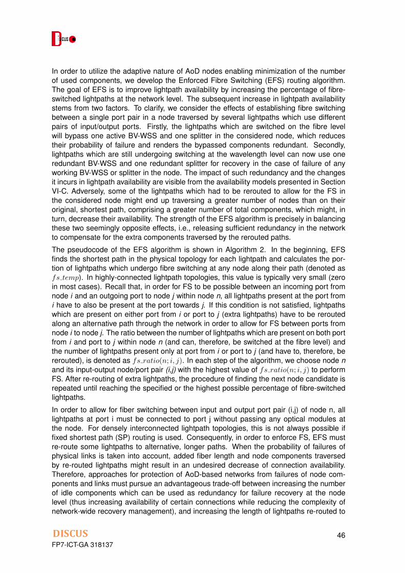
In order to utilize the adaptive nature of AoD nodes enabling minimization of the numberof used components, we develop the Enforced Fibre Switching (EFS) routing algorithm.The goal of EFS is to improve lightpath availability by increasing the percentage of fibre-switched lightpaths at the network level. The subsequent increase in lightpath availabilitystems from two factors. To clarify, we consider the effects of establishing fibre switchingbetween a single port pair in a node traversed by several lightpaths which use differentpairs of input/output ports. Firstly, the lightpaths which are switched on the fibre levelwill bypass one active BV-WSS and one splitter in the considered node, which reducestheir probability of failure and renders the bypassed components redundant. Secondly,lightpaths which are still undergoing switching at the wavelength level can now use oneredundant BV-WSS and one redundant splitter for recovery in the case of failure of anyworking BV-WSS or splitter in the node. The impact of such redundancy and the changesit incurs in lightpath availability are visible from the availability models presented in SectionVI-C. Adversely, some of the lightpaths which had to be rerouted to allow for the FS inthe considered node might end up traversing a greater number of nodes than on theiroriginal, shortest path, comprising a greater number of total components, which might, inturn, decrease their availability. The strength of the EFS algorithm is precisely in balancingthese two seemingly opposite effects, i.e., releasing sufficient redundancy in the networkto compensate for the extra components traversed by the rerouted paths.

The pseudocode of the EFS algorithm is shown in Algorithm 2. In the beginning, EFSfinds the shortest path in the physical topology for each lightpath and calculates the por-tion of lightpaths which undergo fibre switching at any node along their path (denoted asfs temp). In highly-connected lightpath topologies, this value is typically very small (zeroin most cases). Recall that, in order for FS to be possible between an incoming port fromnode i and an outgoing port to node j within node n, all lightpaths present at the port fromi have to also be present at the port towards j. If this condition is not satisfied, lightpathswhich are present on either port from i or port to j (extra lightpaths) have to be reroutedalong an alternative path through the network in order to allow for FS between ports fromnode i to node j. The ratio between the number of lightpaths which are present on both portfrom i and port to j within node n (and can, therefore, be switched at the fibre level) andthe number of lightpaths present only at port from i or port to j (and have to, therefore, bererouted), is denoted as fs ratio(n; i, j). In each step of the algorithm, we choose node nand its input-output node/port pair (i,j) with the highest value of fs ratio(n; i, j) to performFS. After re-routing of extra lightpaths, the procedure of finding the next node candidate isrepeated until reaching the specified or the highest possible percentage of fibre-switchedlightpaths.

In order to allow for fiber switching between input and output port pair (i,j) of node n, alllightpaths at port i must be connected to port j without passing any optical modules atthe node. For densely interconnected lightpath topologies, this is not always possible iffixed shortest path (SP) routing is used. Consequently, in order to enforce FS, EFS mustre-route some lightpaths to alternative, longer paths. When the probability of failures ofphysical links is taken into account, added fiber length and node components traversedby re-routed lightpaths might result in an undesired decrease of connection availability.Therefore, approaches for protection of AoD-based networks from failures of node com-ponents and links must pursue an advantageous trade-off between increasing the numberof idle components which can be used as redundancy for failure recovery at the nodelevel (thus increasing availability of certain connections while reducing the complexity ofnetwork-wide recovery management), and increasing the length of lightpaths re-routed to

FP7-ICT-GA 31813746

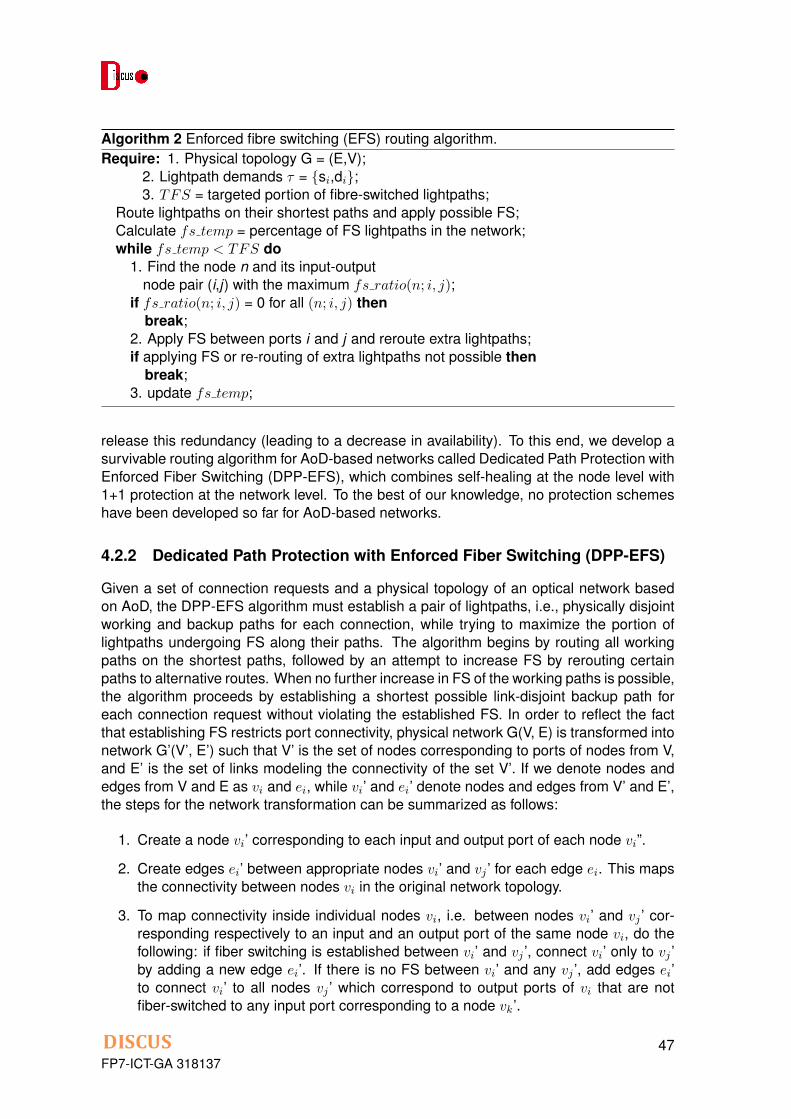
Algorithm 2 Enforced fibre switching (EFS) routing algorithm.Require: 1. Physical topology G = (E,V);

2. Lightpath demands ⌧ = {si,di};3. TFS = targeted portion of fibre-switched lightpaths;

Route lightpaths on their shortest paths and apply possible FS;Calculate fs temp = percentage of FS lightpaths in the network;while fs temp < TFS do

1. Find the node n and its input-outputnode pair (i,j) with the maximum fs ratio(n; i, j);

if fs ratio(n; i, j) = 0 for all (n; i, j) thenbreak;

2. Apply FS between ports i and j and reroute extra lightpaths;if applying FS or re-routing of extra lightpaths not possible then

break;3. update fs temp;

release this redundancy (leading to a decrease in availability). To this end, we develop asurvivable routing algorithm for AoD-based networks called Dedicated Path Protection withEnforced Fiber Switching (DPP-EFS), which combines self-healing at the node level with1+1 protection at the network level. To the best of our knowledge, no protection schemeshave been developed so far for AoD-based networks.

4.2.2 Dedicated Path Protection with Enforced Fiber Switching (DPP-EFS)

Given a set of connection requests and a physical topology of an optical network basedon AoD, the DPP-EFS algorithm must establish a pair of lightpaths, i.e., physically disjointworking and backup paths for each connection, while trying to maximize the portion oflightpaths undergoing FS along their paths. The algorithm begins by routing all workingpaths on the shortest paths, followed by an attempt to increase FS by rerouting certainpaths to alternative routes. When no further increase in FS of the working paths is possible,the algorithm proceeds by establishing a shortest possible link-disjoint backup path foreach connection request without violating the established FS. In order to reflect the factthat establishing FS restricts port connectivity, physical network G(V, E) is transformed intonetwork G’(V’, E’) such that V’ is the set of nodes corresponding to ports of nodes from V,and E’ is the set of links modeling the connectivity of the set V’. If we denote nodes andedges from V and E as vi and ei, while vi’ and ei’ denote nodes and edges from V’ and E’,the steps for the network transformation can be summarized as follows:

1. Create a node vi’ corresponding to each input and output port of each node vi”.

2. Create edges ei’ between appropriate nodes vi’ and vj ’ for each edge ei. This mapsthe connectivity between nodes vi in the original network topology.

3. To map connectivity inside individual nodes vi, i.e. between nodes vi’ and vj ’ cor-responding respectively to an input and an output port of the same node vi, do thefollowing: if fiber switching is established between vi’ and vj ’, connect vi’ only to vj ’by adding a new edge ei’. If there is no FS between vi’ and any vj ’, add edges ei’to connect vi’ to all nodes vj ’ which correspond to output ports of vi that are notfiber-switched to any input port corresponding to a node vk’.

FP7-ICT-GA 31813747

An illustrative example of transforming a simple 5-node network is shown in Fig. 4.5. Afterrouting the four lightpaths on the routes shown in the left part of the figure, FS is establishedin nodes B and D. The right part of the figure shows the network after transformation.Vertices 1 to 24 correspond to the input and the output ports of nodes A to E. The redlines denote FS between a pair of input/output ports inside the same network node. Forexample, vertices 5 and 9 of node B correspond to FS ports and are connected only toeach other, because routing any connection from port 5 to any output port but 9 wouldviolate the established FS. The same applies to ports 15 and 18 of node D. On the otherhand, connectivity of ports not connected via FS to any other port is much greater, as canbe seen, e.g., inside node E in the figure.

A

B C

DE1

2

3

4

5

6

7

8

9

10

11

12

13

14

15

16

17

18

19

20

21

22

23

24

A

B C

DEFiber switching:Node B: ports from A to CNode D: ports from C to D

Figure 4.5: Transforming the network to reflect the impact of established FS to port connec-tivity.

After the network is transformed to incorporate the changes in connectivity introduced byFS, the backup path for each connection is found by deleting the nodes and links usedby the working path and running Dijkstra’s algorithm. We then evaluate the impact of theproposed approaches to network availability via simulation.

4.2.3 Numerical results

DPP-EFS was implemented in C++ and evaluated on a country-wide network of Germanywith 11 nodes and 34 bidirectional links (Fig. 4.6 a)). Lightpath requests between nodepairs were created to serve traffic which was generated proportionally to node populationsand inversely proportional to their distances. The total traffic was scaled to model sparserand denser lightpath topologies. The algorithm was tested on 3 different test instances ofeach load. Failures of optical fibers, splitters, BV-WSSs and MEMS mirrors were gener-ated using Monte Carlo simulations with exponentially distributed times to failure and torepair, under failure rates expressed in FIT (1 FIT = 1 failure in 109 hours) and summarizedin Fig. 4.6 b), and a mean time to repair equal to 6 h. We simulated total time of 1010 hoursand measured minimum (s,t) connection availability and mean down time (MDT) of thenetwork, defined as the average number of minutes per year when at least one connectionis in DOWN state due to failures. The results, shown in Fig. 4.7, were compared to anetwork deploying (i) hard-wired (H-W) and (ii) AoD ROADMs with DPP using SP routingfor the working and the backup paths (denoted as DPP-SP). As shown in Fig. 4.7 a), thes,t availability in network deploying AoD under lower traffic load is greater than for H-WROADMs even when SP routing is used, due to the fact that enough components remainidle and can be used for self-healing. When the logical topology becomes fully connected(� 122 lightpaths), applying DPP-SP renders all components in AoD nodes utilized. In

FP7-ICT-GA 31813748

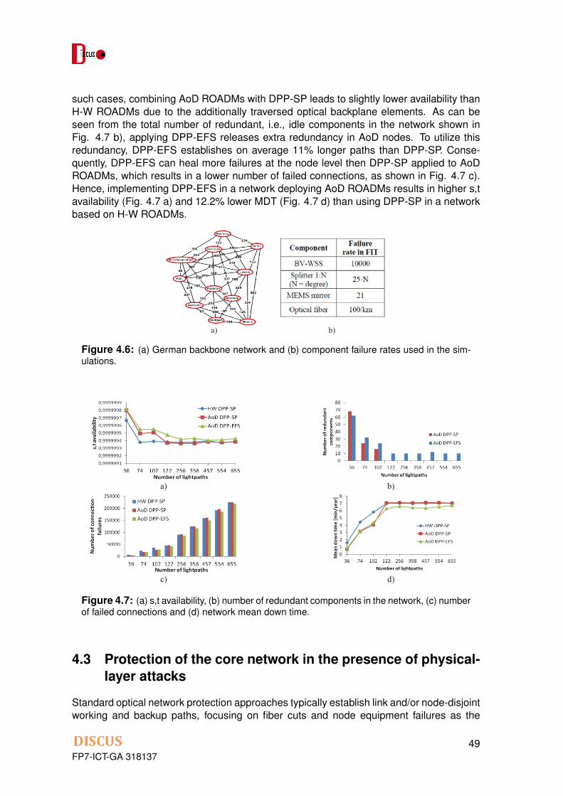
such cases, combining AoD ROADMs with DPP-SP leads to slightly lower availability thanH-W ROADMs due to the additionally traversed optical backplane elements. As can beseen from the total number of redundant, i.e., idle components in the network shown inFig. 4.7 b), applying DPP-EFS releases extra redundancy in AoD nodes. To utilize thisredundancy, DPP-EFS establishes on average 11% longer paths than DPP-SP. Conse-quently, DPP-EFS can heal more failures at the node level then DPP-SP applied to AoDROADMs, which results in a lower number of failed connections, as shown in Fig. 4.7 c).Hence, implementing DPP-EFS in a network deploying AoD ROADMs results in higher s,tavailability (Fig. 4.7 a) and 12.2% lower MDT (Fig. 4.7 d) than using DPP-SP in a networkbased on H-W ROADMs.

a) b)

Figure 4.6: (a) German backbone network and (b) component failure rates used in the sim-ulations.

a) b)

c) d)

Figure 4.7: (a) s,t availability, (b) number of redundant components in the network, (c) numberof failed connections and (d) network mean down time.

4.3 Protection of the core network in the presence of physical-layer attacks

Standard optical network protection approaches typically establish link and/or node-disjointworking and backup paths, focusing on fiber cuts and node equipment failures as the

FP7-ICT-GA 31813749

leading causes of network interruptions. Although effective in the presence of failures,such approaches may not provide adequate protection in the presence of attacks due totheir specific propagation characteristics. A number of optical-layer security breaches andphysical-layer attack methods have been identified in the literature [58], [48], [84], [75],[49], [83], particularly in transparent optical networks. Attacks can induce financial lossesto the clients or cause network-wide service disruption, possibly leading to huge data andrevenue losses for operators. Attacks targeting service degradation, which are in the fo-cus of this study, such as power jamming, typically involve inserting malicious signals intothe network which can potentially propagate along configured connections causing wide-spread damage. To deal with this problem, in this section, we introduce the concept of anAttack Group (AG) defined as a set of connections which can affect each other in case theycarry a malicious attacking signal. A connection is assumed to be attack-protected if itsprimary and backup paths are AG-disjoint. Protecting all connections from attacks couldincur significant resource utilization and may not be economically viable. Thus, we incor-porate attack-awareness into standard link-disjoint dedicated path protection to minimizethe number of attack-unprotected connections only where little or no extra resources arerequired. We refer to the approach as Attack-Aware Dedicated Path Protection (AA-DPP).We develop a 2-step Integer Linear Program (ILP) formulation for AA-DPP, as well as aniterative heuristic for larger instances.

4.3.1 Propagation characteristics of service degradation attacks

Service degradation attacks generally involve inserting malicious signals into the network,such as optical signals of excessive power (e.g., 5-20 dB above other, legitimate signals),to degrade other user connections. Such a signal can be inserted on a legitimate channelused in the network (in-band jamming) or on a wavelength outside the signal window (out-of-band jamming) [83] and can degrade co-propagating user channels due to increasedcrosstalk and nonlinear effects in fibers. Furthermore, a jamming signal can cause so-called gain competition in optical amplifiers where the high-powered signal robs weakerlegitimate signals of gain. Even if electronic equalization in amplifiers counteracts gaincompetition in the steady-state, initial brief oscillations in gain can occur. Additionally, in-band jamming signals can increase intra-channel crosstalk in optical switches to other usersignals traversing the switch on the same wavelength. In a ROADM-based network envi-sioned by DISCUS, a jamming signal would be attenuated at intermediate nodes. However,some propagation may be achieved depending on the strength of the jamming signal andthe working range of the associated VOAs. In Mixed Line Rate and elastic optical networks,an alternative service degradation attack could be achieved by inserting a lower line-rateOOK-modulated signal near a higher line-rate 40/100/200G channel using BPSK, QPSKor DP-QPSK modulation without allowing for enough guardband [49]. This could causeincreased cross phase modulation effects significantly degrading the higher line-rate sig-nals. If such a signal were inserted as a legitimate connection, it could propagate throughthe network degrading all co-propagating neighboring higher-rate channels. Such a signalwould not be thwarted by power equalizing components or even be detected as maliciousby power monitoring equipment.

4.3.2 Attack groups and the considered propagation model

In order to model the propagation characteristics of various attacks and incorporate theminto the protection process, we introduce the concept of an Attack Group (AG). We de-

FP7-ICT-GA 31813750

fine an Attack Group of a working or backup path i, denoted as AG(i), to be comprisedof all other working paths which, if carrying an attacking signal, could potentially degradepath i. Naturally, this depends on the type of attack, its propagation characteristics andphysical routing and wavelength assignment of all the connections in the network. Theconcept of AGs can be applied to individual attacks by considering their distinctive propa-gation characteristics or a combination of them. To cover for the worst-case scenario, weconsider the propagation scenario where an attack inserted on any legitimate connectioncould potentially compromise all other connections sharing common links with it, as well asconnections assigned the same wavelength and traversing common switches with it. Cal-culation of the Attack Groups of individual connections based on our propagation modeland the impact of different path protection schemes is illustrated in Fig. 4.8. Assume fourdirected connection requests: c1:(5-4), c2:(5-6), c3:(4-2) and c4:(6-2); and three availablewavelengths: �

1

, �2

, and �3

. Two different dedicated path protection schemes are shownin Figs. 4.8 a) and 4.8 b), where the working and backup paths of each connection ci aredenoted as cWi and cBi , respectively. In order to find the AG of each connection, we modelattacking relations between connections with a so-called attack graph. In the attack graph,nodes represent the working and backup paths of individual connections and directed linksindicate whether an attacking signal inserted on one of them can affect the other. Note,we assume 1:1 protection where only working paths can be the source of attack.

1

2

6

3

5

4

c1W

c1B

c2W

c2B

c3B

c3W

c4W

c4B

λ1λ2λ3

a) c1W c1

B

c2W

c2B

c3Wc3

B

c4W

c4B

AG(c1W)∩AG(c1

B)={c2W, c3

W}∩{c2W}=c2

W

AG(c2W)∩AG(c2

B)={c1W}∩Ø=Ø

AG(c3W)∩AG(c3

B)={c1W, c4

W}∩{c2W,c4

W}=c4W

AG(c4W)∩AG(c4

B)={c3W}∩Ø=Ø

1

2

6

3

5

4

c1B

c1W

c2W

c2B

c3B

c3Wc4

W

c4B

b) c1W c1

B

c2W

c2B

c3Wc3

B

c4W

c4B

AG(c1W)∩AG(c1

B)=Ø∩{c3W}=Ø

AG(c2W)∩AG(c2

B)=Ø∩{c1W,c3

W,c4W}=Ø

AG(c3W)∩AG(c3

B)={c4W}∩Ø=Ø

AG(c4W)∩AG(c4

B)={c3W}∩{c2

W}=Ø

Figure 4.8: Two possible DPP schemes as their associated attack graphs.

The attack group of a working or backup path is then composed of all the nodes in theattack graph with which it is connected with via incoming links. For example, the attackgroup of working path cW

1

in Fig. 4.8 a) is AG(cW1

) = {cW2

, cW3

}. Namely, connection cW1

could potentially be degraded by an attack inserted on connection cW2

since they share acommon link (5-4), as well as by an attack inserted on cW

3

since they share a commonswitch (4) and are routed on the same wavelength (�

1

). To evaluate whether a connectionis attack-protected, the attack groups of the primary and backup paths should be disjoint.The associated calculations of AG-disjointedness are shown in the figure. We can seethat connection c

1

is not protected because its working and backup paths share a commonAG element, i.e., cW

2

. Similar considerations apply to connection c3

, whose working andbackup paths can both potentially be degraded by an attack inserted on cW

4

. Fig. 4.8 b)shows a slightly different path protection scheme which achieves better attack-protectionwhile using the same number of wavelengths and total path length as the solution in Fig.4.8 a). In Fig. 4.8 b), all connections are attack-protected, i.e. all connections have AG-disjoint working and backup paths.

FP7-ICT-GA 31813751

4.3.3 Attack-Aware Dedicated Path Protection: Problem Definition

Given is a physical topology graph G = (V,E), comprised of a set of nodes V intercon-nected by a set E of directional links. Given are also a set of available wavelengths Wanda set C of connection requests, each defined by their source and destination nodes. TheAttack-Aware Dedicated Path Protection (AA-DPP) problem consists of finding a pair oflink-disjoint paths for each connection request, along with their associated routing andwavelength assignment schemes, while minimizing the number of attack-unprotected con-nections. A connection is assumed attack-unprotected if the working and backup paths ofthe connection are not AG-disjoint according to the attack propagation model describedabove. Due to the high complexity of the AA-DPP problem with the described propagationmodel, we formulate a 2-step ILP which solves the routing and the wavelength assignmentphases subsequently. The routing phase models attacking relations between connectionsharing common links, while the wavelength assignment phase models attacking relationsbetween connection traversing common switches on the same wavelength.

4.3.4 The 2-step ILP formulation (AA-DPP-ILP)

Due to the high complexity of the AA-DPP problem with the described propagation model,we formulate a 2-step ILP which solves the routing and the wavelength assignment phasessubsequently. The routing phase models attacking relations between connection sharingcommon links, while the wavelength assignment phase models attacking relations betweenconnection traversing common switches on the same wavelength. Note, an integrated ILPcould be run by combining the two formulations to find a globally optimal solution butexperimental results indicate that the integrated ILP could only be run in reasonable timefor extremely small instances (4 nodes).

Step 1: The routing phase of AA-DPP-ILP

Notation and parameters:v 2 V : network nodese 2 E: directed network linksoe, te 2 V : the source and destination node of link e, respectivelyc, d 2 C: connection requestsoc, tc 2 V : the source and destination node of connection c, respectivelyH: maximal total hop length

Routing variables:pce = 1 if the working path of connection c uses link e, 0 otherwise.pce = 1 if the backup path of connection c uses link e, 0 otherwise.qcv = 1 if the working path of connection c uses node v, 0 otherwise.qcv = 1 if the backup path of connection c uses node v, 0 otherwise.

Link-sharing and attack-reach variables:lec,d = 1 if the working path of connection c shares link e with the working path of connectiond, 0 otherwise.lec,d = 1 if the backup path of connection c shares link e with the working path of connectiond, 0 otherwise.lc,d = 1 if the working path of connection c shares any link with the working path of con-

FP7-ICT-GA 31813752

nection d, 0 otherwise.lc,d = 1 if the backup path of connection c shares any link with the working path of connec-tion d, 0 otherwise.aLc,d = 1 if the working and the backup path of connection c both share link(s) with theworking path of connection d (and can, thus, be attacked by d on links), 0 otherwise.aLc = 1 if the backup path of connection c is attack-unprotected on links, 0 otherwise.

Objective: minimize the number of attack-unprotected connections under the assumptionthat an attack inserted on a working path can degrade any other working or backup path ifthey share a common link.

minX

c2CaLc (4.39)

Subject to:

8c2C , 8v2V :X

e2E:v=oe,te

pce =

(1 if v = oc or v = tc

2qcv otherwise(4.40)

8c2C , 8v2V :X

e2E:v=oe,te

pce =

(1 if v = oc or v = tc

2qcv otherwise(4.41)

pce + pce 1, 8c2C , 8v2V (4.42)

X

c2C

X

e2Epce + pce H (4.43)

Eqs. 4.40-4.41 define flow conservation and node usage, Eq. 4.42 ensures the workingand back-up paths are link-disjoint and Eq. 4.43 limits the total hop length of all the pathsto H.

lec,d = pce ^ pde , 8e2E , 8c,d2C (4.44)

lec,d = pce ^ pde , 8e2E , 8c,d2C , (4.45)

lc,d =_

e2Elec,d, 8c,d2C (4.46)

lc,d =_

e2Elec,d, 8c,d2C (4.47)

Eqs. 4.44-4.49 of AA-DPP-ILP ensure that if the working and the backup paths of a con-nection c both share links with the working path of any other connection, then connectionc is marked as attack-unprotected. Eqs. 4.44 and 4.45 couple the working and the backuppath of connection c, respectively, to any connection d whose working path shares a linkwith them, while 4.46 and 4.47 mark link-sharing over all connections. For the sake ofbrevity, symbols ^ and _ are used to denote logical AND and OR operations, respectively.

FP7-ICT-GA 31813753

Relation c = a ^ b is implemented as c a; c b; c � a+ b� 1. Similarly, relation c = _iaiis implemented as c � ai, 8i; c

Pi ai.

aLc,d = lc,d ^ lc,d, 8c,d2C (4.48)

aLc =_

d2CaLc,d, 8c,d2C (4.49)

Eq. 4.48 identifies connections c whose both the working and the backup path can beattacked by a connection d, while 4.49 denotes connection c as unprotected if any suchconnection d exists.

Step 2: The wavelength assignment phase of AA-DPP-ILP

In the Wavelength Assignment (WA) phase of AA-DPP-ILP, the values for the routing, link-sharing and attack-reach variables found by solving the routing phase of AA-DPP-ILP areused as input parameters, in addition to the set of nodes, links and connection requests.An additional parameter and the variables for the wavelength assignment phase are asfollows

Notation and parameters:w 2W : Set of available wavelengths

Wavelength assignment variables:rcw = 1 if the working path of c uses wavelength w; 0 otherwise.rcw = 1 if the working path of c uses wavelength w; 0 otherwise.

Switch- and Wavelength-sharing and attack-reach variables:sc,dv,w = 1 if the working path of connection c shares switch v and wavelength w with theworking path of connection d, 0 otherwise.sc,dv,w = 1 if the backup path of connection c shares switch v and wavelength w with theworking path of connection d, 0 otherwise.sc,d = 1 if the working path of connection c shares any common switch and a wavelengthwith the working path of connection d, 0 otherwise.sc,d = 1 if the working path of connection c shares any common switch and a wavelengthwith the working path of connection d, 0 otherwise.aLSc,d = 1 if the working path of d can attack the working path of c on links, and the backuppath of c in switches, 0 otherwise.aSLc,d = 1 if the working path of d can attack the working path of c in switches, and thebackup path of c on links, 0 otherwise.aSc,d = 1 if both the working and the backup path of connection c can be attacked by theworking path of d in switches, 0 otherwise.ac,d = 1 if both the working and the backup path of connection c can be attacked by theworking path of d, 0 otherwise.ac = 1 if connection c is attack-unprotected on links and/or switches, 0 otherwise.

Objective: minimize the number of connections which remain unprotectedfrom attacks(on links or inside switches) according to are assumed propagation model described inSection 4.3.1.

FP7-ICT-GA 31813754

minX

c2Cac (4.50)

Subject to:

X

w2Wrcw = 1, 8c2C (4.51)

X

w2Wrcw = 1, 8c2C (4.52)

X

c2Cpcer

cw +

X

c2Cpcer

cw = 1, 8e2E , 8w2W (4.53)

Equations 4.51-4.53 model the wavelength clash and continuity constraints.

sc,dv,w = qcvrcw ^ qdvr

dw, 8c,d2C , 8v2V , 8w2W (4.54)

sc,dv,w = qcv rcw ^ qdvr

dw, 8c,d2C , 8v2V , 8w2W (4.55)

sc,d =_

v2V,w2Wsc,dv,w, 8c,d2C (4.56)

sc,d =_

v2V,w2Wsc,dv,w, 8c,d2C (4.57)

Eqs. 4.54-4.57 identify wavelength- and switch-sharing among working and backup pathpairs which determine individual attack groups. Eqs. 4.54 and 4.55 couple the workingand the backup path of connection c, respectively, to any connection d whose workingpath shares a wavelength and a switch with them, while 4.56 and 4.57 mark wavelength-and switch-sharing over all connections.

aSc,d = sc,d ^ sc,d, 8c,d2C (4.58)

aSLc,d = sc,d ^ lc,d, 8c,d2C (4.59)

aLSc,d = lc,d ^ sc,d, 8c,d2C (4.60)

ac,d = aSc,d _ aLc,d _ aSLc,d _ aLSc,d , 8c,d2C (4.61)

ac,d =_

d2Cac,d, 8c2C (4.62)

Eqs. 4.58-4.62 identify all possibilities in which the working and the backup path of aconnection c can both be affected by an attacking signal carried on the working path of

FP7-ICT-GA 31813755

a connection d, i.e. check if the working and backup paths of a connection are attackgroup disjoint. Eq. 4.58 identifies connections c whose working and backup paths canboth be attacked by such a connection d in switches. Eq. 4.59 identifies connections cwhose working paths can be attacked by connection d in switches, while its backup pathcan be attacked by connection d in links (and vice versa for 4.60). Eq. 4.61 identifiesconnections c where both the working and backup path can be attacked by a connectiond on links and/or in switches, while 4.62 denotes connection c as attack-unprotected if anysuch connection d exists.

4.3.5 Attack-Aware Dedicated Path Protection heuristic (AA-DPP-H)

For larger problem instances, solving the 2-step AA-DPP-ILP becomes computation-ally intractable. Therefore, we propose an iterative heuristic for attack-aware dedi-cated path protection, denoted as AA-DPP-H. The pseudocode of the AA-DPP-H al-gorithm is shown in Fig. 4.9. As in the ILP, the objective of AA-DPP-H is to mini-mize the number of attack-unprotected connections according to the propagation modeldescribed in Section 4.3.1. Since the heuristic offers more flexibility than the ILP, weapply a secondary objective to minimize the number of working paths that can simul-taneously be affected by a single attack inserted on any one of them, referred to asthe Attack Radius (AR). The AR corresponds to the maximal size of the attack groupof any working path. For example, the AR of the example shown in Fig. 4.8 a) isAR = max{|AG(cW

1

)|, |AG(cW2

)|, |AG(cW3

)|, |AG(cW4

)|} = max{2, 1, 2, 1} = 2. Analo-gously, the AR of the DPP scheme in Fig. 4.8 b) is equal to 1.

The AA-DPP-H algorithm takes as input the physical topology G = (V,E), the number ofavailable wavelengths W , the set of connection requests C, the maximum allowed numberof iterations iMAX , and the number of K shortest paths to be considered as candidateroutes. In the beginning, the incumbent solution, denoted as CSOL, is empty, while thenumber of unprotected connections (UC) and the AR are initialized to a large numericalvalue modeling infinity. The algorithm iteratively constructs a feasible solution CSOL i us-ing a greedy attack-aware approach, and updates the incumbent solution if a more securesolution CSOLi is found. The algorithm ends if a solution where all connections are attackprotected is found or the maximal number of iterations is reached. Details of the construc-tion and evaluation phases are described below.

FP7-ICT-GA 31813756

yes

Input: G=(V,E) //physical topology C //set of connection requests W //set of available wavelengths iMAX //maximum number of iterations K //number of considered shortest paths Initialization: CSOL Å {} //final solution; set of connections with assigned working and backup paths and wavelengths UCÅ∞ //number of connections unprotected from jamming ARÅ∞ //attack radius in the network i = 1 //number of iterations

Evaluate overall security of the solution CSOL_i 28: UC_i Å ∞; 29: For each connection do 30: AG(cW)Å attack group of the working path of c; 31: AG(cB) Å attack group of the backup path of c; 32: If AG(cW) ∩ AG(cB) ≠ Ø then 33: UC_i++; 34: If |AG(cW)| > AR_i then 35: AR_i Å|AG(cW)|; 36: If UC_i < UC or (UC_i == UC and AR_i < AR) then 37: CSOL ÅCSOL_i; AR Å AR_i; UC Å UC_i; 38: i++;

UC>0 and i ≤ iMAX End no

Construct a feasible solution CSOL_i 1: Do 2: CSOL_i Å {}; feasible Åtrue; 3: For each connection do 4: caMIN Å ∞; UCcMIN Å ∞; cWÅ Ø; cBÅ Ø; 5: For each wavelength do 6: cW

w Å set of up to K shortest paths for the working path available on w; 7: If cW

w ≠Ø then 8: For each candidate working path cW

wj do 10: AG(cW

wj) Å attack group of cWwj;

11: AG(cWwj) Å set of backup paths which be attacked by cW

wj; 12: UCc Å|AG(cW

wj) ∩ AG(cWwj)|;

13: For each wavelength do 14: Denote links included in cW

wj as temporarily unavailable on z; 15: cB

z Åset of up to K shortest paths for the backup path on z; 16: If cB

z ≠Ø then 17: For each candidate backup path cB

zk do 18: AG(cB

zk) Åattack group of cBzk;

19: ca Å AG(cWwj) ∩ AG(cB

zk); 20: If ca < caMIN or (ca== caMIN and UCc < UCcMIN) then 21: cWÅ cW

wj; cBÅ cBzk;

22: caÅ caMIN; UCc Å UCcMIN; 23: If cW

≠ Ø and cB ≠ Ø then

24: CSOL_iÅCSOL_i ∪ c; Delete links of cW from w and of cB from z;

25: Else feasible Åfalse; 26: If ⌐feasible then Release all network resources and shuffle set C; 27: While CSOL_i not complete

Figure 4.9: Flow-chart of the AA-DPP algorithm.

Construction phase

In order to construct a feasible solution, the algorithm processes one connection request cat a time while attempting to minimize (i) the number of potential common attackers sharedamong its working path cW and backup path cB (denoted as ca in the pseudocode); and (ii)the number of existing connections whose AG-disjointedness is violated by cW (denoted asUCc). We use a layered graph approach where a copy of the physical topology is made foreach wavelength, and occupied wavelength-links in the current partial solution are deletedfrom their corresponding layers when searching for paths for subsequent requests. Foreach connection request, the approach first searches for up to K available shortest pathcandidates for cW on each available wavelength (row 6). For each cW candidate, denotedas cWwj , the corresponding AG is identified (row 10), as well as the set of existing backuppaths which can be attacked by cWwj , denoted as AG (row 11). The latter is needed tocalculate the value of UCc as the number of elements in the intersection of sets AG andAG (row 12).

The algorithm proceeds by finding a set of up to K shortest path candidates for cB on eachof the available wavelengths, which are link-disjoint with cWwj (row 15). After calculating theAG of each cB candidate, denoted as cBzk (row 18), common potential attackers on cWwj

and cBzk are identified (row 19) and the pair of candidate paths with the minimum value ofca is selected as the solution for cW and cB (row 20). If the value of ca is the same fortwo candidate path pairs, the pair yielding lower UCc value is selected. The combinedpath length of cWwj and cBzk is used as a second tie-breaking rule to prioritize shorter paths(omitted from the pseudocode for the sake of brevity). Finally, if cW and cB are found, theyare added to CSOL i and their links are marked as unavailable on the selected wavelengthsw and z (row 24). If no feasible solution is found all resources are released and set C isshuffled randomly (row 26). The procedure is repeated until a feasible solution CSOL i isfound.

FP7-ICT-GA 31813757

Evaluation phase

In the evaluation phase, the feasible solution found in the construction phase is evalu-ated with respect to the previously described optimization criteria (i.e. number of attack-unprotected connection and the attack radius). The algorithm calculates the AGs for allworking and backup paths (rows 30-31), identifies attack-unprotected connections (rows32-33) and calculates the network AR (rows 34-35). If the current solution CSOL i hasfewer attack-unprotected connections UCi, or the same UCi but a lower AR (row 36), theincumbent solution is updated (row 37).

4.3.6 Simulation results

To evaluate the efficiency of the proposed approaches, they are compared to standardattack-unaware DPP aimed at minimizing the lengths of the established paths and thenumber of wavelengths used. We consider 2 non-attack-aware benchmarking approaches,denoted as DPP-ILP and DPP-H.

DPP-ILP is a 2-step ILP formulation, analogous to AA-DPP-ILP, but instead of minimizingthe number of attack-unprotected connections, the routing phase aims at minimizing thetotal path length used, while the wavelength assignment phase minimizes the number ofwavelengths used. The formulation is derived from formulation AA-DPP-ILP as follows.The link/switch-sharing and attack-reach variables are dropped in both phases, as wellas input parameters H and W . The routing sub-problem of DPP-ILP is then solved withthe objective of minimizing the total length of the established paths, equal to the left-handside of Eq. 4.43, and by considering only constraints 4.40-4.42 from 4.3.4. The WA sub-problem of DPP ILP is aimed at minimizing the number of used wavelengths. Thus, theformulation employs the wavelength assignment variables from 4.3.4 as well as an addi-tional binary variable yw indicating whether wavelength w is used in the final solution. Theobjective is then to minimize the total number of wavelengths used, i.e.

Pw2W yw. The

WA phase is solved by applying the constraints described in Eqs. 4.51-4.53, as well as thefollowing 2 constraints which indicate the wavelengths used:

rcw yw, 8c2C , 8w2W (4.63)

rcw yw, 8c2C , 8w2W (4.64)

DPP-H is a heuristic approach also run as an iterative process with different connectionrequest orderings analogous to AA-DPP-H, but without considering attacks. In every it-eration, it searches for a working and a backup path of all requests with the objective ofminimizing the number of used wavelengths. The working and backup path of each con-nection are assigned the shortest path on the first available wavelength. In every iteration,the algorithm begins by using just one wavelength and adds a new one only when theworking or the backup path cannot fit on any of the previously used wavelengths. At theend of each iteration, the incumbent solution is updated if a solution has been found usingfewer wavelengths, or the same number of wavelengths as the incumbent, but shorter totalpath length.

The 2-step ILP formulations AA-DPP-ILP and DPP-ILP were solved using CPLEX v12.4,while the heuristics AA-DPP-H and DPP-H were implemented as a software tool in C++. All

FP7-ICT-GA 31813758

Seattle

Palo Alto

San Diego

Salt Lake City

BoulderLincoln

Champaign

Houston

Ann Arbor

Ithaca

Pittsburgh

Atlanta

College Pk

Princeton1133

6951715

995569

20951425

721

19731129

2833

750

2350

695

594789

451385

839

367248

Dublin

Glasgow

Oslo

StockholmCopenhagen

Amsterdam

Brussels

Paris

Hamburg

Berlin Warsaw

Munich

London

Frankfurt

Zurich

Lisbon

Bordeaux

MadridBarcelona Milan

Rome

Prague

ViennaBudapest

Zagreb

Kiev

Athens

Marseille

Helsinki

Moscow

503

1588

505444

339

858

515

506

499

1053

5174761024

268302217

349

306489 355

304502

255443

546 895

280

479

392

262

173

343 356463

713 365309 254516

354 809

691

485522

415 396 892

756

2

1

3

4

6

5

7

8a)

b) c)

Figure 4.10: (a) The 8-node, (b) 14-node NSF, and (c) 28-node EON network used in thesimulations.

algorithms were run on an HP workstation equipped with 8 Intel Xeon 2.67 GHz processorsand 16 GB RAM. Three networks were considered, shown in Figure 4.10. Due to thecomplexity of the 2-step attack-aware ILP formulation, AA-DPP-ILP and DPP-ILP wereonly tested for the network shown in Fig. 4.10 a) comprising 8 nodes and 12 bi-directionallinks, each representing two directed links. The AA-DPP-H and DPP-H heuristics wereevaluated on the 8-node network, as well as on the well-known reference networks shownin Figs. 4.10 b) and c) corresponding to the US NSF network (14 nodes, 21 bidirectionallink) and European EON network (28 nodes, 41 bidirectional links), respectively. The trafficfor the 8-node network was generated randomly, with the average logical degree equal to2.86. Traffic for the NSF and EON network was generated based on the node populationand distances, with the average number of lightpaths ranging from 125 to 250.

Fig. 4.11 shows the performance of all the implemented algorithms for the 8-node testcases. Fig. 4.11 a) shows the percentage of attack-unprotected connections for each testcase. AA-DPP-ILP obtains solutions in which all connection are attack-protected, whileAA-DPP-H leaves an average only 7% of connections attack-unprotected. In comparison,the attack-unaware approaches, DPP-ILP and DPP-H, obtain solutions with an averageof 71% and 80% connections attack-unprotected, respectively. Figs. 4.11 b) and c) showresource consumption of the proposed approaches in terms of the total number of hopsin the established paths and the number of used wavelengths. Since the routing phaseof AA-DPP-ILP takes as input the total hop count obtained by the routing phase of DPP-ILP (whose objective is to minimize hop count), both formulations establish solutions withequal hops and are, thus, shown together in the figure. All the approaches gave similarresults with respect to the total average hop count. The wavelength usage in the solutionsobtained was also similar for all the approaches. Since the number of wavelengths usedby DPP-ILP and DPP-H (whose objectives are to minimize wavelengths) were fed as inputparameters to their attack-aware counterparts, they yielded the same number in all thecases tested and are, thus, shown together in the figure.

Fig. 4.12 shows the performance of the heuristics for the NSF and EON test cases. Onaverage, DPP-H leaves more than 80% of connections unprotected from attacks in bothnetworks, while AA-DPP-H reduces the number of vulnerable connections to only 3% in theNSF and 13% in the EON network. Since AA-DPP uses the same number of wavelengthsas wavelength-minimizing DPP while establishing slightly shorter paths, we can concludeit represents a resource-efficient approach of reducing the potential damage from attacks.

FP7-ICT-GA 31813759

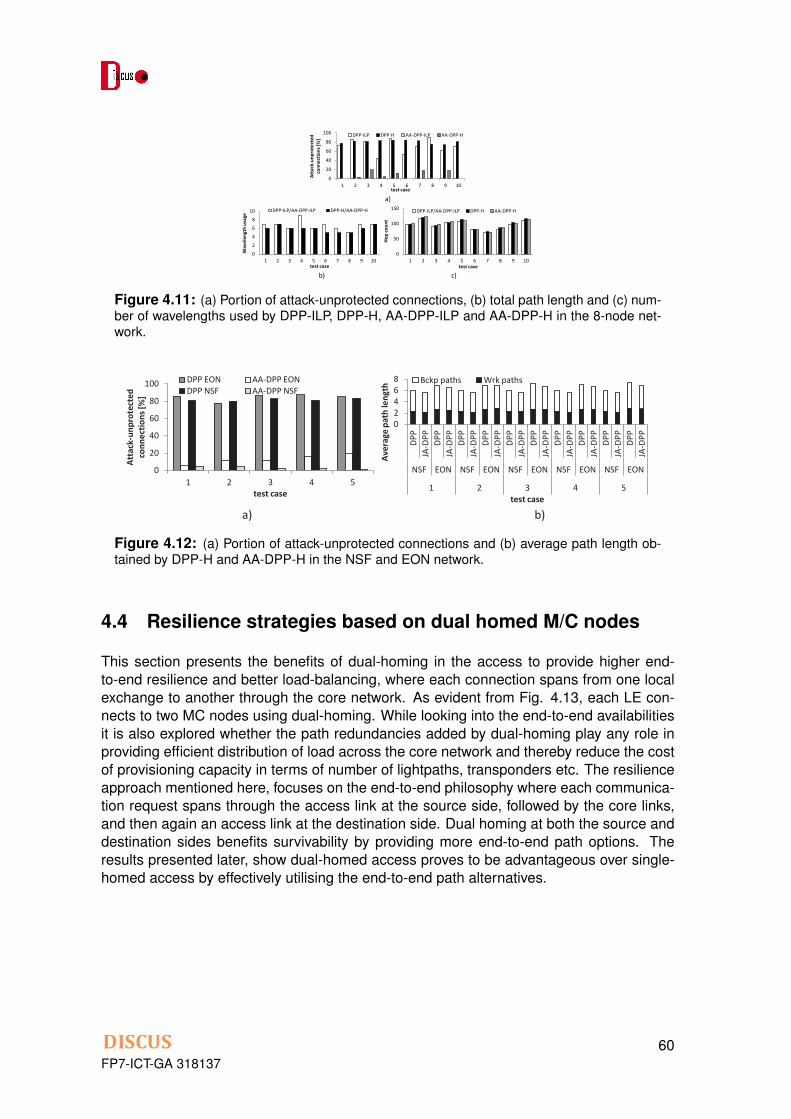
a)

b) c)

0

20

40

60

80

100

1 2 3 4 5 6 7 8 9 10

Atta

ck-u

npro

tect

ed

conn

ectio

ns [%

]

test case

DPP-ILP DPP-H AA-DPP-ILP AA-DPP-H

0

50

100

150

1 2 3 4 5 6 7 8 9 10

Hop

coun

t

test case

DPP-ILP/AA-DPP-ILP DPP-H AA-DPP-H

0 2 4 6 8

10

1 2 3 4 5 6 7 8 9 10

Wav

elen

gth

usag

e

test case

DPP-ILP/AA-DPP-ILP DPP-H/AA-DPP-H

Figure 4.11: (a) Portion of attack-unprotected connections, (b) total path length and (c) num-ber of wavelengths used by DPP-ILP, DPP-H, AA-DPP-ILP and AA-DPP-H in the 8-node net-work.

a) b)

0

20

40

60

80

100

1 2 3 4 5

Atta

ck-u

npro

tect

ed

conn

ectio

ns [%

]

test case

DPP EON AA-DPP EON DPP NSF AA-DPP NSF

0 2 4 6 8

DPP

JA-D

PP

DPP

JA-D

PP

DPP

JA-D

PP

DPP

JA-D

PP

DPP

JA-D

PP

DPP

JA-D

PP

DPP

JA-D

PP

DPP

JA-D

PP

DPP

JA-D

PP

DPP

JA-D

PP

NSF EON NSF EON NSF EON NSF EON NSF EON

1 2 3 4 5

Aver

age

path

leng

th

test case

Bckp paths Wrk paths

Figure 4.12: (a) Portion of attack-unprotected connections and (b) average path length ob-tained by DPP-H and AA-DPP-H in the NSF and EON network.

4.4 Resilience strategies based on dual homed M/C nodes

This section presents the benefits of dual-homing in the access to provide higher end-to-end resilience and better load-balancing, where each connection spans from one localexchange to another through the core network. As evident from Fig. 4.13, each LE con-nects to two MC nodes using dual-homing. While looking into the end-to-end availabilitiesit is also explored whether the path redundancies added by dual-homing play any role inproviding efficient distribution of load across the core network and thereby reduce the costof provisioning capacity in terms of number of lightpaths, transponders etc. The resilienceapproach mentioned here, focuses on the end-to-end philosophy where each communica-tion request spans through the access link at the source side, followed by the core links,and then again an access link at the destination side. Dual homing at both the source anddestination sides benefits survivability by providing more end-to-end path options. Theresults presented later, show dual-homed access proves to be advantageous over single-homed access by effectively utilising the end-to-end path alternatives.

FP7-ICT-GA 31813760

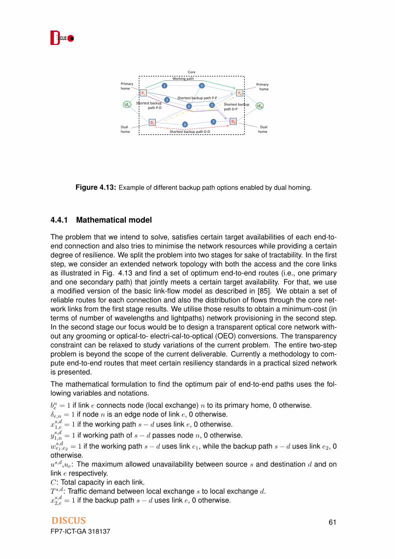
Illustrative example

• LEs = local exchange at the source side; LEd = local exchange at the destination side • P = primary home; D = dual home • The shortest backup path between dual homes on both sides (Ds -Dd) is shorter

than the shortest backup paths between any other combination of the primary and dual homes at the source and destination side (Ps-Pd ,Ps-Dd or Ds-Pd)

1 2

3

4 5

6 7

LEs LEd

Ps

Ds Dd

Pd

Primary home

Dual home

Primary home

Dual home

Working path

Shortest backup path P-P

Shortest backup path D-D

Shortest backup path P-D

Shortest backup path D-P

4

Core

Figure 4.13: Example of different backup path options enabled by dual homing.

4.4.1 Mathematical model

The problem that we intend to solve, satisfies certain target availabilities of each end-to-end connection and also tries to minimise the network resources while providing a certaindegree of resilience. We split the problem into two stages for sake of tractability. In the firststep, we consider an extended network topology with both the access and the core linksas illustrated in Fig. 4.13 and find a set of optimum end-to-end routes (i.e., one primaryand one secondary path) that jointly meets a certain target availability. For that, we usea modified version of the basic link-flow model as described in [85]. We obtain a set ofreliable routes for each connection and also the distribution of flows through the core net-work links from the first stage results. We utilise those results to obtain a minimum-cost (interms of number of wavelengths and lightpaths) network provisioning in the second step.In the second stage our focus would be to design a transparent optical core network with-out any grooming or optical-to- electri-cal-to-optical (OEO) conversions. The transparencyconstraint can be relaxed to study variations of the current problem. The entire two-stepproblem is beyond the scope of the current deliverable. Currently a methodology to com-pute end-to-end routes that meet certain resiliency standards in a practical sized networkis presented.

The mathematical formulation to find the optimum pair of end-to-end paths uses the fol-lowing variables and notations.

bne = 1 if link e connects node (local exchange) n to its primary home, 0 otherwise.�e,n = 1 if node n is an edge node of link e, 0 otherwise.xs,d1,e = 1 if the working path s� d uses link e, 0 otherwise.

ys,d1,n = 1 if working path of s� d passes node n, 0 otherwise.ws,de1,e2 = 1 if the working path s� d uses link e

1

, while the backup path s� d uses link e2

, 0otherwise.us,d,ue: The maximum allowed unavailability between source s and destination d and onlink e respectively.C: Total capacity in each link.T s,d: Traffic demand between local exchange s to local exchange d.xs,d2,e = 1 if the backup path s� d uses link e, 0 otherwise.

FP7-ICT-GA 31813761

ys,d2,n = 1 if the backup path s� d passes node n, 0 otherwise.

The MILP model of the problem is the following.

Objective:Min

X

s,d

X

e2Exs,d1,e + xs,d

2,e (4.65)

Subject to:

X

e2E:�e,n=1

xs,d1,e =

(1 if n = s or n = d

2ys,d1,n otherwise

(4.66)

X

e2E:�e,n=1

xs,d2,e =

(1 if n = s or n = d

2ys,d2,n otherwise

(4.67)

Constraints 4.66-4.67 are flow conservation constraints that maps the flow of links and theassociated nodes.

xs,d1,e 1� bse 8s, d 2 V, e 2 E (4.68)

xs,d1,e 1� bde 8s, d 2 V, e 2 E (4.69)

Constraints 4.68-4.69 denotes that working paths must use the primary homes on bothsource and destination sides, i.e. are not allowed to use feeder fiber which connects it tothe dual home.

xs,d1,e + xs,d

2,e 1 8s, d 2 V, e 2 E (4.70)

Constraint 4.70 accounts for link-disjointedness between primary and backup paths.

X

s,d2V(xs,d

1,e + xs,d2,e) · T

s,d C 8e 2 E (4.71)

X

e12E

X

e22Ews,de1,e2 · ue1 · ue2 us,d 8s, d 2 V (4.72)

Constraint 4.71 enforces the capacity constraint whereas constraint 4.72 is the end-to-endavailability constraint. The MILP provides us with the flow of links that each end-to-endconnection follows through the extended topology including both access and core.

The above ILP model is not scalable for practical network instances because the size ofthe problem is inherently large as we consider an end-to-end topology including the corenetwork as well as thousands of local exchanges. Therefore, we propose a heuristicmodel described in Algorithm 3, to compute the availability-aware routes for each end-to-end connections.

The algorithm takes the extended topology including the MC nodes as well as local ex-changes and their associated connectivities as in-put. It also takes an end-to-end demand

FP7-ICT-GA 31813762

Algorithm 3 Heuristic for Link-Flow ModelInput: End-to-end topology G = (V,E), traffic matrix T =

⇥⇤sd

⇤, set of connections S, link

availabilities set A, core network link capacity upper limit C, target availability At

Output: Set of two disjoint paths between each connection in S meeting target availabilityAt.

1. Sort connections in descending orders based on their demand and put them in a listL.

2. for each connection in L, starting with the first connection, do (a) to (c) until no pathfound

(a) Choose primary-home-to-primary-home path as working path.(b) Reserve capacities for the working path on the intermediate links and update

residual capacities.(c) Sort 4 backup path options based on their ascending hop counts and store them

in list BP .(d) for each of the 4 backup path options of the connection in BP , choose the first

option and do:i. if availability of combination of working and backup path � At, do

A. Check if residual capacities on the links of the chosen backup path cansupport the demand of the connection,

B. If above condition is satisfied, assign the backup path and update thelink capacities of each link in the backup path.

C. Update residual capacities.D. if condition in (A) not satisfied, go to next backup option.

ii. if availability of combination of working and backup path At, go to nextbackup path option.

iii. if availability and capacity condition is not satisfied, return ‘no solution’.

3. calculate total path length for all working and backup paths.

FP7-ICT-GA 31813763

matrix (T), the set of de-mands (S), the link availability set (A), the core network link ca-pacity limit (C), a set of two disjoint shortest paths between each MC node pair, and thetarget availability (At) as input. The output of the algorithm returns a set of two disjointpaths between each connection in S meeting target availability At. The link flow modelheuristic sorts the connections in descending order and for each connection it sets theprimary-home-to-primary-home path for each connection as the working path (as shownin Fig. 4.13). Out of four choices of secondary or backup paths, the heuristic chooses theoptimum path which meets both the link capacity requirement constrained by the capacitylimit C and the target availability requirement i.e., the combined availability of the workingand the backup path should be greater than the target availability At.

4.4.2 Numerical results

The results of dual-homing based resilience heuristic are presented in Table 4.5. The ref-erence topology is a 20-node, 66-link. The different parameters for the illustrative resultson the 6-node topology are as follows: (1) the sustained data rate has been assumed to be10 Mbps per user; (2) the core network is assumed to have a capacity of 80 wavelengthsper fiber with each wavelength carrying 40 Gbps of capacity; (3) The availability per kilo-metre of fiber is used to be 0.999979. End-to-end traffic is calculated using the well-knowngravity model.

We observe that dual homing utilizes the core network resources in a better way thanthe single homing case. The number of hops and the number of links utilized in the dualhoming case is less which is due to the fact that dual homing provides more options forend-to-end routing. Moreover, we also observe that the percentage of connections fallinginto higher availability class is more in case of dual homing than single homing for thesame target availabilities. This proves that dual homing also provides better end-to-endresiliency.

The approach was also tested on a DISCUS UK reference topology and the results areshown in Table 4.6. The UK topology that we have used here is optimized based onminimum fiber distances and it is not always ensured that each MC-node pair has twodisjoint paths. Therefore, some of the end-to-end routes only has one path if we do notconsider dual homing. This degrades the availability considerably as we can notice fromthe table. Dual homing in this case proves to be significantly beneficial as it improves theaverage availabilities and hence the overall resilience.

4.5 Conclusion

In this chapter, we presented planning approaches for providing core-network survivabilityin the presence of single link- and nodefailures, individual node component faults and de-liberate physical-layer attacks targeting service disruption. We developed an abstraction-based design method for increasing the number of node pairs for which there are dis-joint paths of minimized total length and satisfying the signal reach. Compared to thepreliminary network design approaches which did not take resiliency into account, thenew approach brings a significant increase in the number of node pairs connected bydisjoint paths. To account for failures of individual components within nodes, we con-sidered self-healing node architecture based on AoD and proposed a connection routingapproach which alleviates the load of network-level recovery mechanisms by supporting

FP7-ICT-GA 31813764

Scenarios Total LinkUsage

C1(At �0.99999)

C2(0.9999 At <0.99999)

C3(0.999 At <0.9999)

AveragePri-maryHop

AverageSec-ondaryHop

MeanAvailabil-ity

Dual Hom-ing, At =0.99

8901295 14.76% 85.22% 0.014% 6.39 6.05 0.9999784

SingleHoming,At = 0.99

9438945 7.77% 92.23% 0 6.39 6.87 0.9999773


8601283 14.76% 85.22% 0.017% 6.39 6.05 0.9999785


9438945 7.77% 92.23% 0 6.39 6.87 0.9999773


8601270 14.76% 85.24% 0 6.39 6.05 0.9999786


9438945 7.77% 92.23% 0 6.39 6.87 0.9999773

Table 4.5: Dual Homing vs. Single Homing with the Irish topology

Scenarios Total LinkUsage

C1(At �0.99)

AveragePrimaryHop

AverageSec-ondaryHop

MeanAvailability


252746052 100% 6.83 6.44 0.9998


254046744 24.38% 6.83 6.48 0.9848


252890573 100% 6.83 6.44 0.9998


203578793 25.09% 6.83 6.44 0.9923

Table 4.6: Dual Homing vs. Single Homing with the UK topology

FP7-ICT-GA 31813765

node-level recovery. The proposed approach brings a considerable portion of node com-ponent failures that can be healed at the node level and decreases the moan down timein the network. We also developed a protection approach to reduce the potential dam-age from deliberate physical-layer attacks targeting service disruption while maintainingresource-efficiency of standard, resource-minimizing protection approaches which con-sider only component faults. The developed approach dramatically reduces the number ofconnections which remain unprotected in the presence of attacks while requiring no extraresources. Finally, we presented a framework to calculate end-to-end resilient routes for anetwork architecture that consists both of a core network and an extended topology includ-ing access local exchanges. We compared two access architectures viz., dual homing vs.single homing and found that dual homing which has been an efficient resilience techniquein the access can also provide better end-to-end resiliency and efficient load balancing inthe core network.

FP7-ICT-GA 31813766

Chapter 5

Resilient service provisioning

The resiliency work presented in Chapter 4 was mainly focused on design problems (i.e,the traffic matrix describing the services to be provisioned is known before hand). In thischapter we will consider, on the other hand, scenarios where services needs to be pro-visioned on the spot, without any prior knowledge of neither their arrival time nor theirduration (i.e., a dynamic service provisioning scenarios).

Section 5.1 presents a study where the aim is to find hybrid network survivability strate-gies that combine the benefits of both protection- and restoration-based survivable schmes(i.e., high availability with low blocking rate). More specifically, the paper focuses on a dou-ble link failure scenario and proposes two strategies. The first one, couples dedicatedpath protection DPP (1:1) with path restoration (referred to as DPP+PR) to minimize thenumber of dropped connections. The second scheme adds up the concept of backup re-provisioning (BR), referred to as DPP+BR+PR, in order to further increase the connectionavailability achieved by DPP+PR.

Section 5.2 proposes a dynamic connection provisioning strategy which exploits the idleredundant modules use in survivable synthetic ROADMs to support failure recovery. Theintuition behind the proposed approach is to use these modules to provision regular trafficwith the aim of improving the blocking performance of the overall system.

Finally, Section 5.3 presents a heuristic based on the service relocation concept to be usedfor the dynamic restoration of optical cloud services. In other words, upon the occurrenceof a network failure the proposed heuristic solves the routing and resource (i.e., transportplus cloud) allocation problem for each disrupted cloud service allowing, if necessary, torelocate some cloud services to different datacenter nodes.

5.1 Survivability Strategies WDM Networks Offering High Reli-ability Performance

Achieving high reliability performance is a key issue in survivable wavelength division mul-tiplexing (WDM) networks. This is particularly important for mission-critical dynamic ap-plications, where it is crucial to avoid data losses as a consequence of traffic-disruptionscaused by failures. Path-protection-based survivability approaches providing fast recov-ery from fiber cut have been widely studied in the literature and dedicated path protection(DPP) is the most common strategy utilized by network operators, mainly because of itsfast protection switching times [81] as well as its ease of design and implementation. How-ever, path protection schemes are typically designed to provide 100% survivability againstsingle link failures, while the occurrence of multiple link failures will degrade the networkreliability performance. Obviously, adding more backup paths (e.g., DPP 1:N) would im-prove the reliability but it is costly, thus not preferred by network operators. In this context,backup reprovisioning (BR) approaches can be used to protect existing connections andto improve network reliability performance [89, 98]. The key idea is that after the first link

FP7-ICT-GA 31813767

failure, BR is attempted for the vulnerable connections, i.e. the ones left without protection.If any of these connections will be affected by a second failure they will have a new backuppath available. However, BR may not always be effective in multiple link failure scenarios,with total downtime values (i.e., the recovery time, if/when backup resources are available,or alternatively the remaining portion of the service time during which the connection isdown, if a connection cannot recover from a failure) that tend to increase drastically.

This work presented in this section addresses this problem by involving path restoration(PR). We propose two failure recovery schemes, i.e., DPP+PR and DPP+BR+PR providingextra recovery options to vulnerable connections, thus maximizing the average connectionavailability. Time-efficient ILP models (i.e., with computation times less then 50ms) havebeen studied to implement optimal failure recovery for the proposed schemes in a PCE(Path Computation Element)-based [13] WDM network. Results show that, in a double linkfailure scenario, the proposed schemes can achieve higher connection availability, andlower downtime (compared to BR-based approaches), while showing far lower blockingprobability compared to protection strategies based on multiple dedicated backup paths(i.e., DPP 1:2).

5.1.1 Survivable Provisioning Framework and Failure Recovery Schemes

This section first provides a general description of the survivable connection provisioningframework developed in this work. Then it describes the intuition behind the two proposedhybrid survivability schemes, i.e., DPP + PR and DPP + BR + PR. Finally, two additionalschemes, i.e., DPP (1:2) and DPP + BR, used for benchmarking purposes are also in-troduced and described. For space reason the details about the ILP formulation of thevarious schemes are omitted but can be found in [17].

Framework for Survivable Connection Provisioning

The work in this section assumes a dynamic traffic provisioning scenario, where no morethan two failures, regardless of their type, can affect the network simultaneously, i.e., onlya double failure scenario in the network is considered.

Fig. 5.1 illustrates the finite state machine describing the various states in which a con-nection can be when provisioned in the network. Transitions among states are possiblein the presence of specific events: (i) a failure happening in the network, (ii) a failed ele-ment being successfully repaired, (iii) a backup reprovisioning attempt being successful orunsuccessful, and (iv) a path restoration attempt being successfully/unsuccessfully madefor a specific connection. Upon the occurrence of a failure, a connection can find itself ina number of different states depending on what is its current status, the failure recoveryscheme adopted, and on the occurrence of other events (i.e., reparation and/or additionalfailure) in the network. More details are provided next.

According to the proposed framework, a connection is established along with a reserved,dedicated protection path (i.e., DPP). This guarantees the ability to survive to at leastone failure, i.e., the connection is in a PROTECTED state. If a failure affects a protectedconnection, then a transition to the VULNERABLE state takes place. This state is usedto characterize a connection that is still working normally but it is vulnerable against apossible additional failure striking the network, i.e., while already another failure is underreparation. Note that a connection ends up in the VULNERABLE state regardless of which

FP7-ICT-GA 31813768

two proposed hybrid survivability schemes, i.e., DPP! PRand DPP! BR! PR. Finally, two additional schemes, i.e.,DPP (1∶2) and DPP! BR, used for benchmarking purposesare also introduced and described.

A. Framework for Survivable ConnectionProvisioning

The work in this paper assumes a dynamic traffic provi-sioning scenario, where no more than two failures, regard-less of their type, can affect the network simultaneously, i.e.,only a double failure scenario in the network is considered.

Figure 1 illustrates the finite state machine describingthe various states in which a connection can be when provi-sioned in the network. Transitions among states arepossible in the presence of specific events: i) a failure hap-pening in thenetwork, ii) a failed element being successfullyrepaired, iii) a backup reprovisioning attempt beingsuccessful or unsuccessful, and iv) a path restorationattempt being successfully/unsuccessfully made for aspecific connection. Upon the occurrence of a failure, a con-nection can find itself in a number of different states,depending on its current status, the failure recovery schemeadopted, and the occurrence of other events (i.e., reparationand/or additional failure) in the network. More details areprovided next.

According to the proposed framework, a connection is es-tablished along with a reserved, dedicated protection path

(i.e., DPP). This guarantees the ability to survive at leastone failure, i.e., the connection is in a PROTECTED state.If a failure affects a protected connection, then a transitionto the VULNERABLE state takes place. This state is usedto characterize a connection that is still working normallybut is vulnerable to a possible additional failure strikingthe network, i.e., while another failure is already underreparation. Note that a connection ends up in theVULNERABLE state regardless of which path (i.e., pri-mary or backup) is affected by the failure. One possibilityto get back to the PROTECTED state is via a backup repro-visioning attempt. If the attempt is not successful (i.e., lackof wavelength resources), then the connection stays in theVULNERABLE state until the failure is repaired. In themeantime, if another failure affects this vulnerable connec-tion, then a transition to the FAILED state takes place.This state is used to represent a connection that is inter-rupted, i.e., the services provisioned via this connectionare down. At this point, two options are available to getback to the VULNERABLE state. The first one is to doa path restoration attempt. If path restoration is not suc-cessful (i.e., lack of wavelength resources) then the connec-tion ends up in the DROPPED state. Once a connection isdropped, it cannot be recovered and its wavelength resour-ces are released. Restoration is chosen in this frameworkfor its reactive nature and for its inherent ability to effi-ciently use wavelength resources, i.e., backup paths arecomputed only after a failure occurs, and no backup resour-ces are reserved beforehand. The other option to go back tothe VULNERABLE state is to just wait until one of the twofailures is repaired. This option might not always be viable,especially for services with strict downtime requirements.

Using the framework described so far it is possible topropose a number of hybrid survivability schemes thatcombine one or more of the transition options justdescribed. The choice depends on which performance mea-sure (i.e., number of dropped connections versus averageconnection downtime versus efficient use of networkresources) or combination of them is to be addressed.In this paper we propose specifically two survivabilityschemes: DPP! PR and DPP! BR! PR.

Finally, the last two survivability schemes described inthis section, i.e., DPP (1∶2) and DPP! BR, will be used inSection IV for benchmarking purposes.

B. Dedicated Path Protection + Path Restoration

The DPP! PR scheme tries to minimize the number ofdropped connections while limiting the occupied wave-length resources overall in the network. This is achievedby attempting path restoration each time a connection isin the FAILED state but no backup reprovisioning isattempted in any case. On the other hand, as it wasalreadypointedout, path restorationdoesnot giveanyguar-antee of success, especially at a medium or high networkload where wavelength resources might become scarce. Inaddition, the recovery time of path restoration is relativelylong. Both of these aspects are addressed in the schemedescribed next.

Fig. 1. Finite state machine showing the possible states of aconnection and the type of transition a connection can experiencewhile provisioned in the network.

A154 J. OPT. COMMUN. NETW./VOL. 5, NO. 10/OCTOBER 2013 Ahmed et al.

Figure 5.1: Finite State Machine showing: the possible states of a connection and the typeof transition a connection can experience while provisioned in the network.

path (i.e., primary or backup) is affected by the failure. One possibility to get back to thePROTECTED state is via a backup reprovisioning attempt. If the attempt is not successful(i.e., lack of wavelength resources) then the connection stays in the VULNERABLE stateuntil the failure is repaired. In the meantime, if another failure affects this vulnerable con-nection, then a transition to the FAILED state takes place. This state is used to represent aconnection that is interrupted, i.e., the services provisioned via this connection are down.At this point two options are available to get back to the VULNERABLE state. The first oneis to do a path restoration attempt. If path restoration is not successful (i.e., lack of wave-length resources) then the connection ends up in the DROPPED state. Once a connectionis dropped, it cannot be recovered and its wavelength resources are released. Restorationis chosen in this framework for its reactive nature and for its inherent ability to efficientlyuse wavelength resources, i.e., backup paths are computed only after a failure occurs, andno backup resources are reserved beforehand. The other option to go back to the VUL-NERABLE state is to just wait until one of the two failures is repaired. This option mightnot be always viable, especially for services with strict downtime requirements.Using the framework described so far it is possible to propose a number of hybrid surviv-ability schemes that combine one or more of the transitions options just described. Thechoice depends on which performance measure (i.e., number of dropped connections vs.average connection downtime vs. efficient use of network resources) or combination ofthem is to be addressed. In this section we propose specifically two survivability schemes,i.e. DPP + PR and DPP + BR + PR. Finally, the last two survivability schemes describedin this section, i.e., DPP (1:2) and DPP + BR, will be used for benchmarking purposes.Dedicated Path Protection + Path Restoration (DPP + PR). The DPP + PR schemetries to minimize the number of dropped connections while limiting the amount of occu-pied wavelength resources overall in the network. This is achieved by attempting path

FP7-ICT-GA 31813769

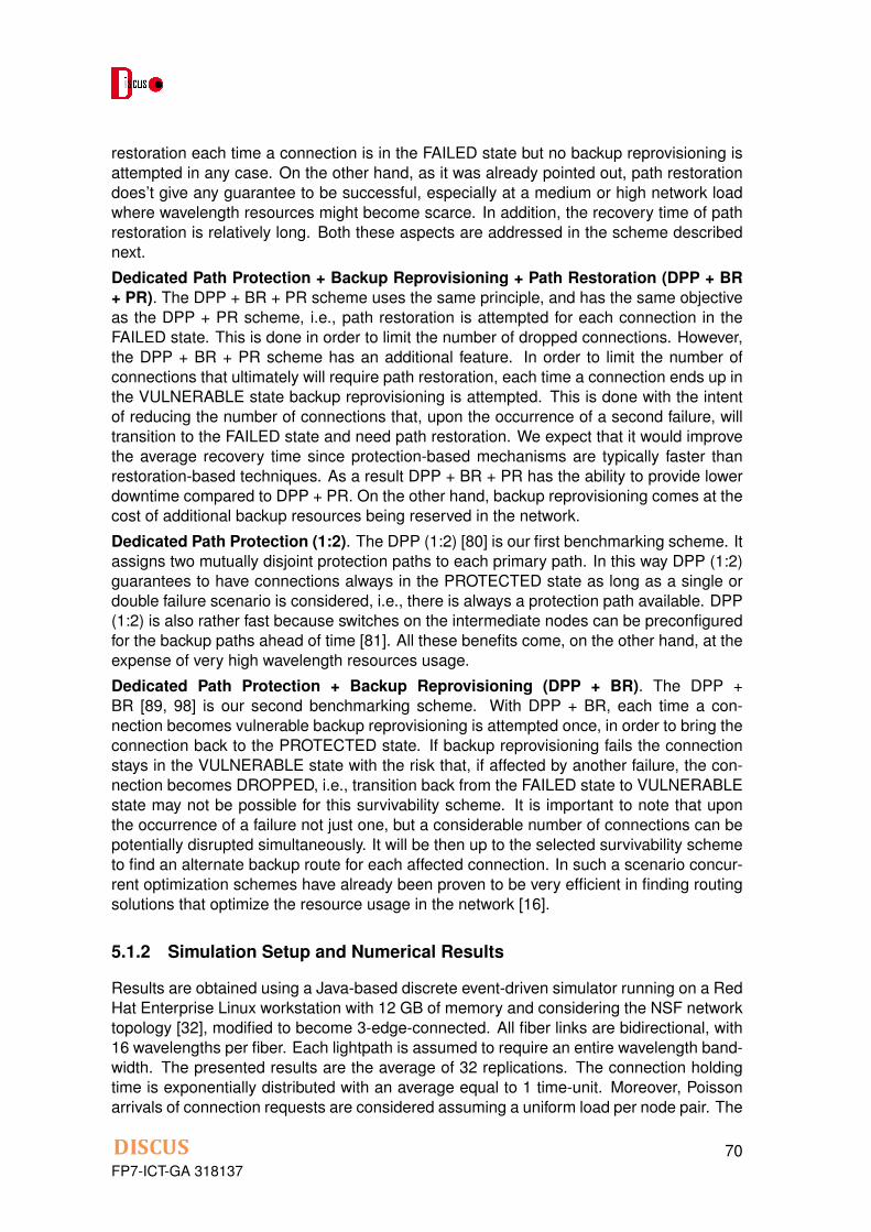
restoration each time a connection is in the FAILED state but no backup reprovisioning isattempted in any case. On the other hand, as it was already pointed out, path restorationdoes’t give any guarantee to be successful, especially at a medium or high network loadwhere wavelength resources might become scarce. In addition, the recovery time of pathrestoration is relatively long. Both these aspects are addressed in the scheme describednext.Dedicated Path Protection + Backup Reprovisioning + Path Restoration (DPP + BR+ PR). The DPP + BR + PR scheme uses the same principle, and has the same objectiveas the DPP + PR scheme, i.e., path restoration is attempted for each connection in theFAILED state. This is done in order to limit the number of dropped connections. However,the DPP + BR + PR scheme has an additional feature. In order to limit the number ofconnections that ultimately will require path restoration, each time a connection ends up inthe VULNERABLE state backup reprovisioning is attempted. This is done with the intentof reducing the number of connections that, upon the occurrence of a second failure, willtransition to the FAILED state and need path restoration. We expect that it would improvethe average recovery time since protection-based mechanisms are typically faster thanrestoration-based techniques. As a result DPP + BR + PR has the ability to provide lowerdowntime compared to DPP + PR. On the other hand, backup reprovisioning comes at thecost of additional backup resources being reserved in the network.Dedicated Path Protection (1:2). The DPP (1:2) [80] is our first benchmarking scheme. Itassigns two mutually disjoint protection paths to each primary path. In this way DPP (1:2)guarantees to have connections always in the PROTECTED state as long as a single ordouble failure scenario is considered, i.e., there is always a protection path available. DPP(1:2) is also rather fast because switches on the intermediate nodes can be preconfiguredfor the backup paths ahead of time [81]. All these benefits come, on the other hand, at theexpense of very high wavelength resources usage.Dedicated Path Protection + Backup Reprovisioning (DPP + BR). The DPP +BR [89, 98] is our second benchmarking scheme. With DPP + BR, each time a con-nection becomes vulnerable backup reprovisioning is attempted once, in order to bring theconnection back to the PROTECTED state. If backup reprovisioning fails the connectionstays in the VULNERABLE state with the risk that, if affected by another failure, the con-nection becomes DROPPED, i.e., transition back from the FAILED state to VULNERABLEstate may not be possible for this survivability scheme. It is important to note that uponthe occurrence of a failure not just one, but a considerable number of connections can bepotentially disrupted simultaneously. It will be then up to the selected survivability schemeto find an alternate backup route for each affected connection. In such a scenario concur-rent optimization schemes have already been proven to be very efficient in finding routingsolutions that optimize the resource usage in the network [16].

5.1.2 Simulation Setup and Numerical Results

Results are obtained using a Java-based discrete event-driven simulator running on a RedHat Enterprise Linux workstation with 12 GB of memory and considering the NSF networktopology [32], modified to become 3-edge-connected. All fiber links are bidirectional, with16 wavelengths per fiber. Each lightpath is assumed to require an entire wavelength band-width. The presented results are the average of 32 replications. The connection holdingtime is exponentially distributed with an average equal to 1 time-unit. Moreover, Poissonarrivals of connection requests are considered assuming a uniform load per node pair. The

FP7-ICT-GA 31813770

connected. All fiber links are bidirectional, with 16 wavelengths per fiber. Each lightpath is assumed to require an entire wavelength bandwidth. The presented results are the average of 32 replications. The connection holding time is exponentially distributed with an average equal to 1 time-unit. Moreover, Poisson arrivals of connection requests are considered assuming a uniform load per node pair. The ILP models are solved using the Gurobi Optimizer 4.51 [6]. Time between failures occurring in the whole network is assumed to be exponentially distributed with an average equal to 2.5 time-units. Mean time to repair (MTTR) of a broken link is considered to be equal to 0.5 time-units. For dynamic DPP 1:1 connection provisioning, the heuristic presented in [7] is used. During failure recovery, the original primary path is restored back after a failed link is repaired.. α, β, γ1 and γ2 in the ILP objective functions are assumed to be 10,000, 1.0, 0.5 and 0.25 respectively, for the reasons explained in the previous section.

20 40 60 80 1000.01

0.1

1

10

100

20 40 60 80 100

1

10

100

400

20 40 60 80 100

1E-4

1E-3

0.01

0.1

20 40 60 80 100

100

200

300

400

500

600

Bloc

king

Pro

babl

ity [%

]

(a) Load [Erlangs]

DPP + PR DPP + BR + PR DPP 1:2 DPP + BR

Avg

. Con

nec.

Dro

pped

[#]

(b) Load [Erlangs]

DPP + PR DPP + BR + PR DPP + BR

Avg

. Con

nec.

Una

vaila

bilit

y [%

]

(c) Load [Erlangs]


Wav

elen

gth

Reso

urce

Usa

ge [#

]

(d) Load [Erlangs]

DPP + PR (Primary) DPP + PR (Backup) DPP + BR + PR (Primary) DPP + BR + PR (Backup) DPP 1:2 (Primary) DPP 1:2 (Backup) DPP + BR (Primary) DPP + BR (Backup)

Fig.1. (a) Blocking Probability, (b) Avg. # of Dropped Connections, (c) Avg. Connection Unavailability, (d), Number of Used Wavelengths.

DPP+PR DPP+BR+PR DPP+BR Load [Erlangs] 20 60 100 20 60 100 20 60 100

Downtime [time-units] 0.415 5.31 17.56 0.345 3.34 8.68 273 284 309 Table.1. Total connection downtime for different schemes.

Fig. 1(a) shows that the blocking probability (BP) is substantially higher for DPP 1:2 because it provisions three mutually link-disjoint paths (one primary and two backups) per each connection. It is also shown that DPP+BR+PR has slightly worse BP performance compared to DPP+PR because of the BR operations. DPP+PR drops almost twice as many connections as DPP+BR+PR (Fig. 1(b)), but still, both DPP+PR and DPP+BR+PR have a substantially fewer number of connections dropped than DPP+BR. Both proposed schemes show low connection unavailability values (Fig. 1(c)) which are worse than DPP 1:2, but way better than DPP+BR. Finally (Fig. 1(d)), DPP 1:2 requires significantly more backup resources as compared to the two proposed schemes. The total connection downtime values, in low load conditions, are very small for both the proposed schemes, but they grow more rapidly for DPP+PR at higher loads (i.e., 60-100 Erlangs). The reason is that DPP+BR+PR utilizes BR first to minimize the downtime, and PR is only attempted as a last-resort to avoid dropping a connection. On the other hand, the total connection downtime for DPP 1:2 can be neglected since it is equal to the switching time of an automatic optical switch, as a protection path for a provisioned connection is always guaranteed. 4. Conclusion Two dynamic failure recovery schemes for PCE-based WDM networks (incl. ILP models) are proposed and evaluated against two benchmark schemes, i.e., DPP 1:2 and DPP+BR. In a double link failure scenario, the proposed schemes, i.e., DPP+PR and DPP+BR+PR, show a substantially better BP performance compared to DPP 1:2, while still being able to achieve significantly lower connection unavailability values than DPP+BR. Finally, DPP+BR+PR shows low total connection downtime values, and drops only half as many connections as DPP+PR in high network load conditions, an important performance criterion for network service providers. References [1] S. Ramamurthy, et. al., IEEE/OSA Journal of Lightwave Technology, 21, 870- (2003). [2] L. Song, et. al., IEEE/ACM Transactions on Networking, vol.16, no.6, pp.1366-1377, December, 2008. [3] J. Zhang et. al., IEEE Journal on Selected Areas in Communications, vol.24, no.8, pp.57-67, August, 2006. [4] A. Farrel, et al., “A Path Computation Element (PCE) Based Architecture”, IETF RFC 4655, August, 2006. [5] X.-W. Chu, et al., in Proc. of IEEE INFOCOM 2003. San Francisco, CA, USA, April, 2003. [6] Gurobi Optimizer, Online URL: http://www.gurobi.com/. [7] J. Ahmed, et. al., in Proc. of NOC/OC&I 2009, Valladolid, Spain, June 2009.

Figure 5.2: Blocking Probability (a), Avg. # of Dropped Connections (b), Avg. ConnectionUnavailability (c), Number of Used Wavelengths (d) as a function of the network load.

ILP models are solved using the Gurobi Optimizer 4.51 [1]. Time between failures occur-ring in the whole network is assumed to be exponentially distributed with an average equalto 2.5 time-units. Mean time to repair (MTTR) of a broken link is considered to be equalto 0.5 time-units. For dynamic DPP 1:1 connection provisioning, the heuristic presentedin [18] is used. During failure recovery, the original primary path is restored back after afailed link is repaired. ↵, �, �1 and �2 in the ILP objective functions presented in [17] areassumed to be 10,000, 1.0, 0.5 and 0.25 respectively.

Fig. 5.2(a) shows that the blocking probability (BP) is substantially higher for DPP 1:2 be-cause it provisions three mutually link-disjoint paths (one primary and two backups) pereach connection. It is also shown that DPP+BR+PR has slightly worse BP performancecompared to DPP+PR because of the BR operations. DPP+PR drops almost twice asmany connections as DPP+BR+PR (Fig. 5.2(b)), but still, both DPP+PR and DPP+BR+PRhave a substantially fewer number of connections dropped than DPP+BR. Both proposedschemes show low connection unavailability values (Fig. 5.2(c)) which are worse thanDPP 1:2, but way better than DPP+BR. Finally (Fig. 5.2(d)), DPP 1:2 requires significantlymore backup resources as compared to the two proposed schemes. The table reported inFig. 5.3 shows the connection downtime values experienced when using different failurerecovery schemes. The connection downtime is defined as the time in which a connectionis not in normal working conditions because of a protection switching event, a restora-tion attempt being under way, or because of the connection being dropped. As can beexpected from the connection unavailability results presented in Fig. 5.2(c), the DPP+BRscheme shows the worst downtime values because of the lack of any dynamic restorationprocedure to recover from a failure after an unsuccessful backup reprovisioning attempt.On the other hand, the DPP + PR and the DPP + BR + PR schemes show much lowerdowntime values. Note that the downtime results for DPP (1:2) are not shown becauseof their negligible values since the only time a connection is down is during protectionswitching.

FP7-ICT-GA 31813771

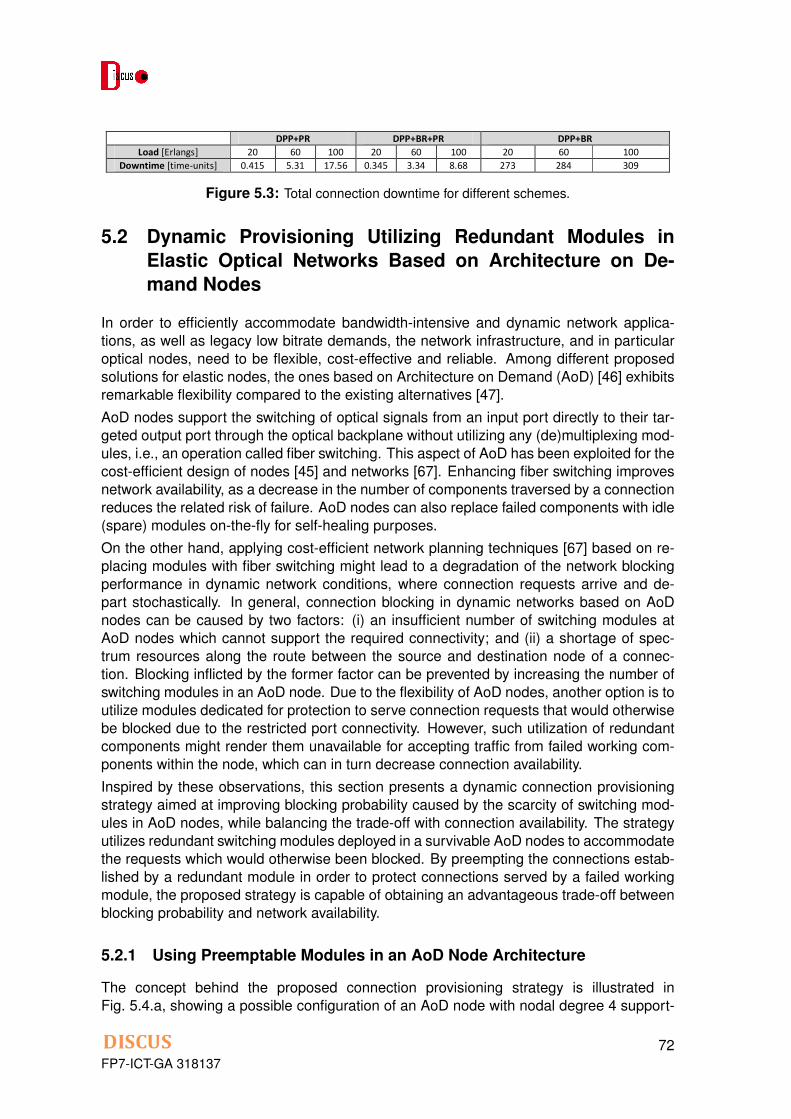
connected. All fiber links are bidirectional, with 16 wavelengths per fiber. Each lightpath is assumed to require an entire wavelength bandwidth. The presented results are the average of 32 replications. The connection holding time is exponentially distributed with an average equal to 1 time-unit. Moreover, Poisson arrivals of connection requests are considered assuming a uniform load per node pair. The ILP models are solved using the Gurobi Optimizer 4.51 [6]. Time between failures occurring in the whole network is assumed to be exponentially distributed with an average equal to 2.5 time-units. Mean time to repair (MTTR) of a broken link is considered to be equal to 0.5 time-units. For dynamic DPP 1:1 connection provisioning, the heuristic presented in [7] is used. During failure recovery, the original primary path is restored back after a failed link is repaired.. α, β, γ1 and γ2 in the ILP objective functions are assumed to be 10,000, 1.0, 0.5 and 0.25 respectively, for the reasons explained in the previous section.

20 40 60 80 1000.01

0.1

1

10

100

20 40 60 80 100

1

10

100

400

20 40 60 80 100

1E-4

1E-3

0.01

0.1

20 40 60 80 100

100

200

300

400

500

600

Bloc

king

Pro

babl

ity [%

]

(a) Load [Erlangs]


Avg

. Con

nec.

Dro

pped

[#]

(b) Load [Erlangs]

DPP + PR DPP + BR + PR DPP + BR

Avg

. Con

nec.

Una

vaila

bilit

y [%

](c) Load [Erlangs]


Wav

elen

gth

Reso

urce

Usa

ge [#

]

(d) Load [Erlangs]

DPP + PR (Primary) DPP + PR (Backup) DPP + BR + PR (Primary) DPP + BR + PR (Backup) DPP 1:2 (Primary) DPP 1:2 (Backup) DPP + BR (Primary) DPP + BR (Backup)

Fig.1. (a) Blocking Probability, (b) Avg. # of Dropped Connections, (c) Avg. Connection Unavailability, (d), Number of Used Wavelengths.

DPP+PR DPP+BR+PR DPP+BR Load [Erlangs] 20 60 100 20 60 100 20 60 100

Downtime [time-units] 0.415 5.31 17.56 0.345 3.34 8.68 273 284 309 Table.1. Total connection downtime for different schemes.

Fig. 1(a) shows that the blocking probability (BP) is substantially higher for DPP 1:2 because it provisions three mutually link-disjoint paths (one primary and two backups) per each connection. It is also shown that DPP+BR+PR has slightly worse BP performance compared to DPP+PR because of the BR operations. DPP+PR drops almost twice as many connections as DPP+BR+PR (Fig. 1(b)), but still, both DPP+PR and DPP+BR+PR have a substantially fewer number of connections dropped than DPP+BR. Both proposed schemes show low connection unavailability values (Fig. 1(c)) which are worse than DPP 1:2, but way better than DPP+BR. Finally (Fig. 1(d)), DPP 1:2 requires significantly more backup resources as compared to the two proposed schemes. The total connection downtime values, in low load conditions, are very small for both the proposed schemes, but they grow more rapidly for DPP+PR at higher loads (i.e., 60-100 Erlangs). The reason is that DPP+BR+PR utilizes BR first to minimize the downtime, and PR is only attempted as a last-resort to avoid dropping a connection. On the other hand, the total connection downtime for DPP 1:2 can be neglected since it is equal to the switching time of an automatic optical switch, as a protection path for a provisioned connection is always guaranteed. 4. Conclusion Two dynamic failure recovery schemes for PCE-based WDM networks (incl. ILP models) are proposed and evaluated against two benchmark schemes, i.e., DPP 1:2 and DPP+BR. In a double link failure scenario, the proposed schemes, i.e., DPP+PR and DPP+BR+PR, show a substantially better BP performance compared to DPP 1:2, while still being able to achieve significantly lower connection unavailability values than DPP+BR. Finally, DPP+BR+PR shows low total connection downtime values, and drops only half as many connections as DPP+PR in high network load conditions, an important performance criterion for network service providers. References [1] S. Ramamurthy, et. al., IEEE/OSA Journal of Lightwave Technology, 21, 870- (2003). [2] L. Song, et. al., IEEE/ACM Transactions on Networking, vol.16, no.6, pp.1366-1377, December, 2008. [3] J. Zhang et. al., IEEE Journal on Selected Areas in Communications, vol.24, no.8, pp.57-67, August, 2006. [4] A. Farrel, et al., “A Path Computation Element (PCE) Based Architecture”, IETF RFC 4655, August, 2006. [5] X.-W. Chu, et al., in Proc. of IEEE INFOCOM 2003. San Francisco, CA, USA, April, 2003. [6] Gurobi Optimizer, Online URL: http://www.gurobi.com/. [7] J. Ahmed, et. al., in Proc. of NOC/OC&I 2009, Valladolid, Spain, June 2009.

Figure 5.3: Total connection downtime for different schemes.

5.2 Dynamic Provisioning Utilizing Redundant Modules inElastic Optical Networks Based on Architecture on De-mand Nodes

In order to efficiently accommodate bandwidth-intensive and dynamic network applica-tions, as well as legacy low bitrate demands, the network infrastructure, and in particularoptical nodes, need to be flexible, cost-effective and reliable. Among different proposedsolutions for elastic nodes, the ones based on Architecture on Demand (AoD) [46] exhibitsremarkable flexibility compared to the existing alternatives [47].AoD nodes support the switching of optical signals from an input port directly to their tar-geted output port through the optical backplane without utilizing any (de)multiplexing mod-ules, i.e., an operation called fiber switching. This aspect of AoD has been exploited for thecost-efficient design of nodes [45] and networks [67]. Enhancing fiber switching improvesnetwork availability, as a decrease in the number of components traversed by a connectionreduces the related risk of failure. AoD nodes can also replace failed components with idle(spare) modules on-the-fly for self-healing purposes.On the other hand, applying cost-efficient network planning techniques [67] based on re-placing modules with fiber switching might lead to a degradation of the network blockingperformance in dynamic network conditions, where connection requests arrive and de-part stochastically. In general, connection blocking in dynamic networks based on AoDnodes can be caused by two factors: (i) an insufficient number of switching modules atAoD nodes which cannot support the required connectivity; and (ii) a shortage of spec-trum resources along the route between the source and destination node of a connec-tion. Blocking inflicted by the former factor can be prevented by increasing the number ofswitching modules in an AoD node. Due to the flexibility of AoD nodes, another option is toutilize modules dedicated for protection to serve connection requests that would otherwisebe blocked due to the restricted port connectivity. However, such utilization of redundantcomponents might render them unavailable for accepting traffic from failed working com-ponents within the node, which can in turn decrease connection availability.Inspired by these observations, this section presents a dynamic connection provisioningstrategy aimed at improving blocking probability caused by the scarcity of switching mod-ules in AoD nodes, while balancing the trade-off with connection availability. The strategyutilizes redundant switching modules deployed in a survivable AoD nodes to accommodatethe requests which would otherwise been blocked. By preempting the connections estab-lished by a redundant module in order to protect connections served by a failed workingmodule, the proposed strategy is capable of obtaining an advantageous trade-off betweenblocking probability and network availability.

5.2.1 Using Preemptable Modules in an AoD Node Architecture

The concept behind the proposed connection provisioning strategy is illustrated inFig. 5.4.a, showing a possible configuration of an AoD node with nodal degree 4 support-

FP7-ICT-GA 31813772

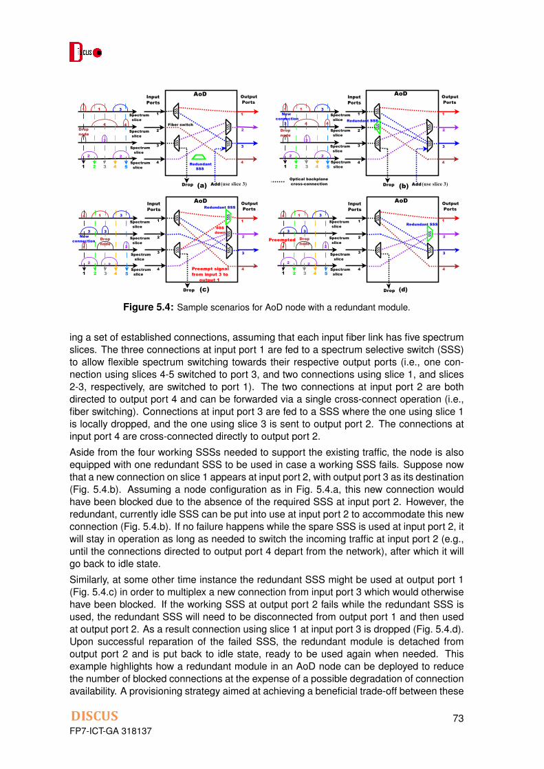
Figure 5.4: Sample scenarios for AoD node with a redundant module.

ing a set of established connections, assuming that each input fiber link has five spectrumslices. The three connections at input port 1 are fed to a spectrum selective switch (SSS)to allow flexible spectrum switching towards their respective output ports (i.e., one con-nection using slices 4-5 switched to port 3, and two connections using slice 1, and slices2-3, respectively, are switched to port 1). The two connections at input port 2 are bothdirected to output port 4 and can be forwarded via a single cross-connect operation (i.e.,fiber switching). Connections at input port 3 are fed to a SSS where the one using slice 1is locally dropped, and the one using slice 3 is sent to output port 2. The connections atinput port 4 are cross-connected directly to output port 2.Aside from the four working SSSs needed to support the existing traffic, the node is alsoequipped with one redundant SSS to be used in case a working SSS fails. Suppose nowthat a new connection on slice 1 appears at input port 2, with output port 3 as its destination(Fig. 5.4.b). Assuming a node configuration as in Fig. 5.4.a, this new connection wouldhave been blocked due to the absence of the required SSS at input port 2. However, theredundant, currently idle SSS can be put into use at input port 2 to accommodate this newconnection (Fig. 5.4.b). If no failure happens while the spare SSS is used at input port 2, itwill stay in operation as long as needed to switch the incoming traffic at input port 2 (e.g.,until the connections directed to output port 4 depart from the network), after which it willgo back to idle state.Similarly, at some other time instance the redundant SSS might be used at output port 1(Fig. 5.4.c) in order to multiplex a new connection from input port 3 which would otherwisehave been blocked. If the working SSS at output port 2 fails while the redundant SSS isused, the redundant SSS will need to be disconnected from output port 1 and then usedat output port 2. As a result connection using slice 1 at input port 3 is dropped (Fig. 5.4.d).Upon successful reparation of the failed SSS, the redundant module is detached fromoutput port 2 and is put back to idle state, ready to be used again when needed. Thisexample highlights how a redundant module in an AoD node can be deployed to reducethe number of blocked connections at the expense of a possible degradation of connectionavailability. A provisioning strategy aimed at achieving a beneficial trade-off between these

FP7-ICT-GA 31813773

two objectives is presented next.

5.2.2 Dynamic Provisioning with Preemptable Spectrum Selective Switches(DP-PSSS)

This section describes how the concept of preemptable modules introduced in the previ-ous section can be integrated in a dynamic provisioning strategy for AoD-based opticalnetworks.The connection set-up strategy presented in this section (i.e., Dynamic Provisioning withPreemptable Spectrum Selective Switches, or DP-PSSS) works as follows. Given thesource and the destination node of a connection to be set up, DP-PSSS checks, for eachroute within a set of pre-computed k-shortest paths candidate, if all the AoD nodes tra-versed by a candidate path are capable to switch the signal from the required input to therequired output port. Note that once fiber switching is used to connect an input port i withan output port j at a given node, it is no longer possible to switch signals from port i to anyoutput port different from j as long as the connection(s) that is (are) fiber-switched betweenports i and j are active. If the required connectivity at a given node along a candidate routeis not supported due to fiber switching, DP-PSSS checks if there is an idle redundant SSSin that node. If yes, then the redundant SSS is used to switch the connection. If no spareSSSs are available, the candidate path is removed from further consideration. If there areno viable candidate paths for the current request, the connection is blocked. Otherwise,the spectrum availability is checked on each of the viable candidate paths. If free, continu-ous, and contiguous spectrum slices are found, the path remains a viable candidate routefor provisioning the connection request. Among all the viable candidate routes, the onethat requires a smaller number of new, previously unused SSSs is selected.

5.2.3 Numerical Results

A custom-built event-driven simulator is used to study the performance of the DP-PSSSstrategy. Simulations are carried out on the NSF topology [42], with 14 nodes and 42unidirectional fiber links, each supporting 80 spectrum slices. It is assumed that onlysingle SSS failure can occur in the network, i.e., the probability that two or more SSSswill fail at the same time is considered to be negligible. Connections are assumed toarrive in the network following a Poisson process, each one requiring a number of slicesuniformly distributed among {2, 4, 6, 8} with an exponentially distributed duration, whoseaverage value is set to 1 time unit. Source/destination pairs of connection requests areassumed to be uniformly distributed among all nodes. The number of candidate paths foreach connection request is set to 5. The performance of DP-PSSS is assessed in termsof the number of demands rejected due to a limited number of switching modules at AoDnodes, and in terms of average connection availability. Results are compared against abenchmark strategy that works exactly as DP-PSSS, but does not allow using redundantSSSs to provision regular traffic. The presented results are averaged over fifty experimentsfor each traffic load value.The number of active SSSs initially placed at each node is determined by the offline de-sign procedure described in [42], where the network is dimensioned differently for eachspecific traffic condition. This translates in an overall number of switching modules in thenetwork that is relatively small for low loads, and increases for higher load values. Suchapproach avoids over-provisioning of switching modules in nodes when and where they

FP7-ICT-GA 31813774

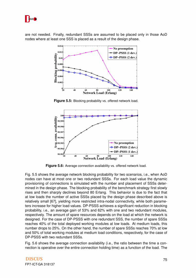
are not needed. Finally, redundant SSSs are assumed to be placed only in those AoDnodes where at least one SSS is placed as a result of the design phase.

20 40 60 80 100 120 1400

0.002

0.004

0.006

0.008

0.01

0.012

0.014

Network Load (Erlang)

Blo

ckin

g p

rob

ab

ilit

y

No preemption

DP−PSSS (1 dev.)

DP−PSSS (2 dev.)

Figure 5.5: Blocking probability vs. offered network load.

20 40 60 80 100 120 14099.993

99.994

99.995

99.996

99.997

99.998

99.999

100

Network Load (Erlang)

Avg. co

nn

. avail

ab

ilit

y

No preemption

DP−PSSS (2 dev.)

DP−PSSS (1 dev.)

Figure 5.6: Average connection availability vs. offered network load.

Fig. 5.5 shows the average network blocking probability for two scenarios, i.e., when AoDnodes can have at most one or two redundant SSSs. For each load value the dynamicprovisioning of connections is simulated with the number and placement of SSSs deter-mined in the design phase. The blocking probability of the benchmark strategy first slowlyrises and then sharply declines beyond 80 Erlang. This behavior is due to the fact thatat low loads the number of active SSSs placed by the design phase described above isrelatively small [67], yielding more restricted intra-nodal connectivity, while both parame-ters increase for higher load values. DP-PSSS achieves a significant reduction in blockingprobability, i.e., an average gain of 53% and 62% with one and two redundant modules,respectively. The amount of spare resources depends on the load at which the network isdesigned. For the case of DP-PSSS with one redundant SSS, the number of spare SSSsreaches 40% of the total deployed working modules at low loads. At medium loads, thisnumber drops to 25%. On the other hand, the number of spare SSSs reaches 70% at lowand 50% of total working modules at medium load conditions, respectively, for the case ofDP-PSSS with two redundant SSSs.

Fig. 5.6 shows the average connection availability (i.e., the ratio between the time a con-nection is operative over the entire connection holding time) as a function of the load. The

FP7-ICT-GA 31813775

benchmark strategy, which employs the redundant resources only for failure recovery dis-plays 100% availability. The lower blocking obtained by DP-PSSS comes at the expenseof slightly degraded availability due to preemption of connections which traverse a backupSSS in the event of a working module failure. However, this degradation is relatively con-tained, as it is shown that the average value of the connection availability never dropsbelow four nines.

5.3 Restoring Optical Cloud Services with Service Relocation

The optical cloud is a very popular concept by which storage and computing resources,also referred to as IT resources, are spread over different datacenter (DC) locations in-terconnected via high-speed optical wavelength division multiplexing (WDM) links. In thisparadigm cloud services are provisioned in an anycast fashion, where only the sourcenode needs to be specified in the routing and resource assignment phase, while any ofthe DCs can be used to accommodate a cloud service, as long as its IT resource require-ments are met. Anycast provisioning has a number of advantages already recognized byoptical cloud providers [36, 37]. It allows, for example, for the live relocation of those cloudservices that are already provisioned, i.e., a concept also known as service relocation. Ifthe DC location is not essential while provisioning a certain cloud service, it becomes thenpossible to relocate the job over multiple DC locations. This allows for a more efficientmanagement of both cloud and transport network resources. There are also energy ben-efits that might derive from relocating, whenever possible, a service in a DC powered bygreen energy source [62].Service relocation has also the potential to bring an extra degree of flexibility to surviv-ability strategies. In fact, by opportunely relocating a cloud service it is possible to usea protection path terminating at a DC that is different from the one used by the primarypath. These benefits have been assessed in the literature showing the ability of servicerelocation to improve resource efficiency when used in conjunction with path protectionstrategies [37]. Another instance in which service relocation might be beneficial is whenit is combined with restoration-based survivability strategies. These strategies are veryefficient in the way they use backup resources, i.e., they are dynamically provisioned onlyupon a failure, but restoration-based approaches suffer from a certain risk that the backupnetwork resources might not be available when needed [17]. Service relocation can poten-tially alleviate this problem. Our preliminary study in this direction confirms that relocatinga cloud service disrupted by a network failure is beneficial in terms of both restorabilityand average connection availability [19]. The results in [19] are based on the solution of aninteger linear programming (ILP) model, which is fairly complex and does not scale well.In order to fully assess the benefits of combining the cloud service relocation concept withrestoration, we proposed, in addition to the ILP formulation [19], an efficient and scal-able heuristic algorithm. A simple but powerful strategy was developed, able to jointlysolve the restoration and service relocation problem. The proposed heuristic, calledH RELOCATION and presented in this section, selects for each failed cloud servicethe best combination of IT and network resources such that the number of restored cloudservices is maximized, while the number of cloud service that need relocation is mini-mized. Simulation results show that the performance of H RELOCATION in terms ofboth restorability and average connection availability is very close to the optimal result ob-tained by the ILP formulation used as a benchmark [19], while offering a significant gain interms of processing time.

FP7-ICT-GA 31813776

close to the optimal result obtained by the ILP formulation used as a benchmark [5], while offering a significant gain in terms of processing time.

2. RESTORATION WITH SERVICE RELOCATION HEURISTIC

This section first describes the restoration with service relocation problem and then presents a heuristic (i.e., H_RELOCATION) specifically tailored to solve it.

Let G(N,E) be the graph describing the status of the optical transport network after the occurrence of a failure (i.e., where the failed network element(s) are not included in the graph representation). In this work only a single failure scenario is considered, but the problem and the proposed heuristic can be easily extended to a multi-failure scenario. G(N,E) consists of N nodes and E fiber links. NDC represents the set of datacenters nodes (NDC ⊂ N) each one having 𝐷𝐶𝑘

𝑠𝑡 available storage units, and 𝐷𝐶𝑘

𝑝𝑢 available processing units, with DCk ∈ NDC. Let Q be the set of disrupted cloud services that need to be restored after the occurrence of a failure in the network, each one (Qi ∈ Q) requiring 𝑄𝑖

𝑠𝑡 storage units and 𝑄𝑖𝑝𝑢 processing units. The source

node of Qi is si, while di represents the DC node serving Qi before the failure. The auxiliary variable curRoute is used to store the temporary best route to a cloud service.

The objective of the restoration with service relocation problem is to maximize the number of recovered cloud services Qi ∈ Q while minimizing the number of service relocations. A heuristic, which solves this problem, is presented next.

The H_RELOCATION heuristic is described in

Fig. 1. In the figure the shortestPath function returns the shortest available (i.e., with available wavelengths) path between two given nodes out of a set of pre-computed k shortest paths between them. If no such path exists or if there are no available wavelength resources on any of the pre-computed paths the shortestPath function returns NULL. The function

hopCount returns the number of hops of a given route, or MAX_VALUE when curRoute=NULL.

H_RELOCATION tries to restore each cloud service Qi ∈ Q sequentially. For each Qi the heuristic first checks if there is an available path in G(N,E) from si to the DC already in use (i.e., di). This is done to reduce the number of unnecessary service relocations. If no such path exists H_RELOCATION tries to find an alternative DC with enough storage (i. e. , 𝑄𝑖

𝑠𝑡) and computing (i.e., 𝑄𝑖

𝑝𝑢) resources able to accommodate Qi. If more than one DC with enough resources is reachable, the heuristic chooses the one that is the closest to si in terms of hop count. Once the new DC is selected the cloud service is relocated and a lightpath from si to the new DC is established. In case neither a suitable DC nor an available path to it can be found, the cloud service is dropped.

3. PERFORMANCE ASSESSMENT This section describes the scenario used to assess the performance of the H_RELOCATION heuristic, and then discusses a number of simulation results. 3.1 Scenario and assumptions The NSF network (Fig. 2) is considered as a reference topology [5], where nodes 3, 4, 10 and 11 are assumed to be DC nodes due to their high connectivity. Each DC is equipped with 3000 storage units and 150 processing units. All fiber links in the network are bidirectional, comprising 16 wavelengths each (with the exception of

Input: G(N, E), NDC, Qi �Q and network state Output: selectedRoute if path is provisioned else NULL Auxiliary: curRoute := NULL

1: if ((selectedRoute := shortestPath(si, di)) != NULL) return selectedRoute; 2: for each DCk ∈ NDC | (𝐷𝐶𝑘

𝑠𝑡 >= 𝑄𝑖𝑠𝑡)∧(𝐷𝐶𝑘

𝑣𝑚 >= 𝑄𝑖𝑣𝑚)

3: curRoute := shortestPath(si, DCk); 4: if (hopCount(curRoute) < hopCount(selectedRoute)) selectedRoute := curRoute; 5: if (selectedRoute = NULL) return NULL; 6: else return selectedRoute;

Fig. 1: Pseudo-code for H_RELOCATION heuristic

Fig. 2: NSF topology with 4 DCs

1

2

3

5

6

7

8

9

11

12

13

14

104

Figure 5.7: Pseudo-code for H RELOCATION heuristic.

5.3.1 Restoration with Service Relocation Heuristic

This section first describes the restoration with service relocation problem and thenpresents a heuristic (i.e., H RELOCATION ) specifically tailored to solve it. Let G(N,E)be the graph describing the status of the optical transport network after the occurrence ofa failure (i.e., where the failed network element(s) are not included in the graph represen-tation). In this work only a single failure scenario is considered, but the problem and theproposed heuristic can be easily extended to a multi-failure scenario. G(N,E) consistsof N nodes and E fiber links. NDC represents the set of datacenters nodes (NDC ⇢ N )each one having DCk

st available storage units, and DCkpu available processing units, with

DCk ⇢ NDC . Let Q be the set of disrupted cloud services that need to be restored af-ter the occurrence of a failure in the network, each one (Qi ⇢ Q) requiring Qi

st storageunits and Qi

pu processing units. The source node of Qi is si, while di represents the DCnode serving Qi before the failure. The auxiliary variable curRoute is used to store thetemporary best route to a cloud service.

The objective of the restoration with service relocation problem is to maximize the numberof recovered cloud services Qi ⇢ Q while minimizing the number of service relocations.The remainder of the section presents a heuristic which solves this problem.

The H RELOCATION heuristic is described in Fig. 5.7. In the figure the shortestPathfunction returns the shortest available (i.e., with available wavelengths) path between twogiven nodes out of a set of pre-computed k shortest paths between them. If no such pathexists or if there are no available wavelength resources on any of the pre-computed pathsthe shortestPath function returns NULL. The function hopCount returns the number ofhops of a given route, or MAX V ALUE when curRoute=NULL.

H RELOCATION tries to restore each cloud service Qi ⇢ Q sequentially. For each Qi

the heuristic first checks if there is an available path in G(N,E) from si to the DC already inuse (i.e., di). This is done to reduce the number of unnecessary service relocations. If nosuch path exists H RELOCATION tries to find an alternative DC with enough storage(i.e.,Qi

st) and computing (i.e., Qipu) resources able to accommodate Qi. If more than one

DC with enough resources is reachable, the heuristic chooses the one that is the closestto si in terms of hop count. Once the new DC is selected the cloud service is relocated

FP7-ICT-GA 31813777

close to the optimal result obtained by the ILP formulation used as a benchmark [5], while offering a significant gain in terms of processing time.

2. RESTORATION WITH SERVICE RELOCATION HEURISTIC

This section first describes the restoration with service relocation problem and then presents a heuristic (i.e., H_RELOCATION) specifically tailored to solve it.

Let G(N,E) be the graph describing the status of the optical transport network after the occurrence of a failure (i.e., where the failed network element(s) are not included in the graph representation). In this work only a single failure scenario is considered, but the problem and the proposed heuristic can be easily extended to a multi-failure scenario. G(N,E) consists of N nodes and E fiber links. NDC represents the set of datacenters nodes (NDC ⊂ N) each one having 𝐷𝐶𝑘

𝑠𝑡 available storage units, and 𝐷𝐶𝑘

𝑝𝑢 available processing units, with DCk ∈ NDC. Let Q be the set of disrupted cloud services that need to be restored after the occurrence of a failure in the network, each one (Qi ∈ Q) requiring 𝑄𝑖

𝑠𝑡 storage units and 𝑄𝑖𝑝𝑢 processing units. The source

node of Qi is si, while di represents the DC node serving Qi before the failure. The auxiliary variable curRoute is used to store the temporary best route to a cloud service.

The objective of the restoration with service relocation problem is to maximize the number of recovered cloud services Qi ∈ Q while minimizing the number of service relocations. A heuristic, which solves this problem, is presented next.

The H_RELOCATION heuristic is described in

Fig. 1. In the figure the shortestPath function returns the shortest available (i.e., with available wavelengths) path between two given nodes out of a set of pre-computed k shortest paths between them. If no such path exists or if there are no available wavelength resources on any of the pre-computed paths the shortestPath function returns NULL. The function

hopCount returns the number of hops of a given route, or MAX_VALUE when curRoute=NULL.

H_RELOCATION tries to restore each cloud service Qi ∈ Q sequentially. For each Qi the heuristic first checks if there is an available path in G(N,E) from si to the DC already in use (i.e., di). This is done to reduce the number of unnecessary service relocations. If no such path exists H_RELOCATION tries to find an alternative DC with enough storage (i. e. , 𝑄𝑖

𝑠𝑡) and computing (i.e., 𝑄𝑖

𝑝𝑢) resources able to accommodate Qi. If more than one DC with enough resources is reachable, the heuristic chooses the one that is the closest to si in terms of hop count. Once the new DC is selected the cloud service is relocated and a lightpath from si to the new DC is established. In case neither a suitable DC nor an available path to it can be found, the cloud service is dropped.

3. PERFORMANCE ASSESSMENT This section describes the scenario used to assess the performance of the H_RELOCATION heuristic, and then discusses a number of simulation results. 3.1 Scenario and assumptions The NSF network (Fig. 2) is considered as a reference topology [5], where nodes 3, 4, 10 and 11 are assumed to be DC nodes due to their high connectivity. Each DC is equipped with 3000 storage units and 150 processing units. All fiber links in the network are bidirectional, comprising 16 wavelengths each (with the exception of

Input: G(N, E), NDC, Qi �Q and network state Output: selectedRoute if path is provisioned else NULL Auxiliary: curRoute := NULL

1: if ((selectedRoute := shortestPath(si, di)) != NULL) return selectedRoute; 2: for each DCk ∈ NDC | (𝐷𝐶𝑘

𝑠𝑡 >= 𝑄𝑖𝑠𝑡)∧(𝐷𝐶𝑘

𝑣𝑚 >= 𝑄𝑖𝑣𝑚)

3: curRoute := shortestPath(si, DCk); 4: if (hopCount(curRoute) < hopCount(selectedRoute)) selectedRoute := curRoute; 5: if (selectedRoute = NULL) return NULL; 6: else return selectedRoute;

Fig. 1: Pseudo-code for H_RELOCATION heuristic

Fig. 2: NSF topology with 4 DCs

1

2

3

5

6

7

8

9

11

12

13

14

104

Figure 5.8: NSF topology with 4 DCs.

and a lightpath from si to the new DC is established. In case neither a suitable DC nor anavailable path to it can be found, the cloud service is dropped.

5.3.2 Performance Assessment

The NSF network (Fig. 5.8) is considered as a reference topology [19], where nodes 3,4, 10 and 11 are assumed to be DC nodes due to their high connectivity. Each DC isequipped with 3000 storage units and 150 processing units. All fiber links in the networkare bidirectional, comprising 16 wavelengths each (with the exception of the link connect-ing each DC to its network node, which have unlimited capacity). All nodes have fullwavelength conversion capability.Each experiment consists of one million anycast cloud services to be provisioned from aclient (i.e., non-DC) node to a DC node (which are uniformly chosen for each cloud service)with enough storage and processing resources, in the interval from 1 to 100 and from 1to 5, respectively. Each cloud service is also assumed to require the entire capacity of awavelength channel.In the normal operating conditions each cloud service is provisioned using theDC CLOSEST heuristic [61], while upon the occurrence of a failure, H RELOCATIONis applied to restore as many cloud services as possible. Each cloud service holding timeis assumed to be exponentially distributed with an average value equal to 60 time-unitswhile service request arrivals at the client nodes follow a Poisson process, with mean timebetween arrivals defined by the current load. Only fiber link failures are considered inthis work. The time between two consecutive failures in the network is exponentially dis-tributed, with a mean value equal to 1000 time units, while the link reparation time, alsoexponential distributed, has a mean time to repair equal to 10 time units.

FP7-ICT-GA 31813778

the link connecting each DC to its network node, which have unlimited capacity). All nodes have full wavelength conversion capability.

Each experiment consists of one million anycast cloud services to be provisioned from a client (i.e., non-DC) node to a DC node (which are uniformly chosen for each cloud service) with enough storage and processing resources, in the interval from 1 to 100 and from 1 to 5, respectively. Each cloud service is also assumed to require the entire capacity of a wavelength channel.

In the normal operating conditions each cloud service is provisioned using the DC_CLOSEST heuristic [6], while upon the occurrence of a failure, H_RELOCATION is applied to restore as many cloud services as possible. Each cloud service holding time is assumed to be exponentially distributed with an average value equal to 60 time-units while service request arrivals at the client nodes follow a Poisson process, with mean time between arrivals defined by the current load. Only fiber link failures are considered in this work. The time between two consecutive failures in the network is exponentially distributed, with a mean value equal to 1000 time units, while the link reparation time, also exponential distributed, has a mean time to repair equal to 10 time units.

All the presented results are the average of 30 different experiments, carried out using a Java-based discrete event-driven simulator [7]. The workstation used is a Red Hat Enterprise Linux with 8 Intel Xeon CPUs (4 cores per CPU) clocked at 2.67 GHz and with 16 GB of RAM memory. The confidence interval of the blocking probability is 5% or lower, with 95% of confidence level, except for the lower loads.

3.2 Performance evaluation In the performance evaluation phase three survivability strategies are used for benchmarking purposes. The first one is a protection strategy for anycast cloud services called Backup Server via Physically disjoint Path (BSPP) [8], while the other two are ILP models representing: (i) an optimal restoration strategy without relocation capabilities (i.e., ILP_PR) [4], and (ii) an optimal restoration strategy with relocation capabilities and minimum number of cloud service relocations (i.e., ILP_RELOCATION) [5].

Figure 3 shows some performance results of the H_RELOCATION strategy as a function of the network load. The first thing that can be noticed is the inherent benefit, in terms of blocking probability (Fig. 3a), when using restoration-based strategies. More than one order of magnitude can be gained at low to medium loads when no dedicated protection resources are assigned. In addition it can also be noticed that using cloud service relocation (and consequently potentially longer restoration paths) has a little impact on the blocking probability. Fig. 3b shows the ratio between the number of successfully recovered cloud services over the total number of recovery attempts (i.e., restorability) as a function of load. As expected, BSPP guarantees 100% recovery against any single failure. However, as shown in Fig.3a, this comes at the expense of very high blocking probability, even in relatively low load conditions. On the other hand, the relocation opportunity is quite efficient in increasing the chances of a cloud service being recovered. In this respect

(a) (b)

(c) (d)

Fig. 3: Simulation results

0,001

0,01

0,1

1

10

100

120 130 140 150 160 170 180 190

Bloc

king

pro

babi

lity

[%]

Load [Erlangs]

BSPPILP_PRILP_PR_RELOCATIONH_RELOCATION

40

50

60

70

80

90

100

120 130 140 150 160 170 180 190

Res

tora

bilit

y [%

]

Load [Erlangs]


99,85

99,87

99,89

99,91

99,93

99,95

99,97

99,99

120 130 140 150 160 170 180 190

Av.

Ava

ilabi

lity

[%]

Load [Erlangs]


0

2

4

6

8

10

12

14

16

120 130 140 150 160 170 180 190

Rel

ocat

ions

[%]

Load [Erlangs]

ILP_PR_RELOCATIONH_RELOCATION

Figure 5.9: Simulation results.

All the presented results are the average of 30 different experiments, carried out usinga Java-based discrete event-driven simulator [15]. The workstation used is a Red HatEnterprise Linux with 8 Intel Xeon CPUs (4 cores per CPU) clocked at 2.67 GHz and with16 GB of RAM memory. The confidence interval of the blocking probability is 5% or lower,with 95% of confidence level, except for the lower loads.

In the performance evaluation phase three survivability strategies are used for bench-marking purposes. The first one is a protection strategy for anycast cloud services calledBackup Server via Physically disjoint Path (BSPP) [86], while the other two are ILP mod-els representing: (i) an optimal restoration strategy without relocation capabilities (i.e.,ILP PR) [17], and (ii) our optimal restoration strategy with relocation capabilities and min-imum number of cloud service relocations (i.e., ILP RELOCATION ) [19].

Fig. 5.9 shows some performance results of the H RELOCATION strategy as a func-tion of the network load. The first thing that can be noticed is the inherent benefit, interms of blocking probability (Fig. 5.9a), when using restoration-based strategies. Morethan one order of magnitude can be gained at low to medium loads when no dedicatedprotection resources are assigned. In addition it can also be noticed that using cloud ser-vice relocation (and consequently potentially longer restoration paths) has a little impacton the blocking probability. Fig. 5.9b shows the ratio between the number of successfullyrecovered cloud services over the total number of recovery attempts (i.e., restorability)as a function of load. As expected, BSPP guarantees 100% recovery against any singlefailure. However, as shown in Fig. 5.9a, this comes at the expense of very high block-ing probability, even in relatively low load conditions. On the other hand, the relocationfeature is quite efficient in increasing the chances of a cloud service being recovered. Inthis respect H RELOCATION presents restorability values that are very close to theoptimal (i.e., ILP RELOCATION ). Similar conclusions can also be drawn while exam-

FP7-ICT-GA 31813779

ining the average connection availability (i.e., the ratio between the time a cloud serviceis operative over the entire cloud service holding time) value shown in Fig 5.9c. In thiscase H RELOCATION is slightly worse than ILP RELOCATION , which is due tothe sequential nature of the heuristic that cannot concurrently optimize the restorationattempt of batch of disrupted cloud services. Finally, Fig 5.9.d shows efficiency of the pro-posed H RELOCATION heuristic in containing the number of required relocations (i.e.,ratio between the number of restored cloud service that required relocation over the totalrestoration attempts) when compared to their minimal value (i.e., ILPPRRELOCATION ).The graph also shows that when the blocking probability is low, the number of relocationsgrows with the load, but after the system saturates, the number of relocations stabilizes,showing that the DCs and network resources are already highly utilized and it is difficult toaccommodate services to be relocated from the affected DC to another DC, which reducesthe number of possible relocations when the load is further increasing.

5.4 Conclusions

This chapter first addressed the problem of guaranteeing high survivability levels in WDMtransport networks in the presence of multiple failures. More specifically, the work focusedon double link failure scenarios and proposes two hybrid survivability schemes, namelyDPP + PR and DPP + BR + PR. These schemes combine the backup reprovisionig (BR)concept with an end-to-end path restoration (PR) scheme with a focus on maximizing theconnection availability without a significant impact on the blocking performance. Thesetwo schemes were evaluated against two benchmark solutions, namely DPP (1:2) andDPP + BR. Simulation results show that both proposed schemes achieve substantiallybetter blocking probability performance than DPP (1:2), while still maintaining acceptableconnection availability levels. Furthermore, their performance in terms of connection avail-ability is far better than DPP+BR. Finally, the DPP + BR + PR scheme results in low con-nection downtime values, and drops only half as many connections as DPP + PR underhigh load, which is an important performance parameter for network service providers.

As a second contribution the chapter presented a dynamic connection provisioning strat-egy for optical networks with programmable ROADMs. The proposed strategy exploitsthe presence of switching modules deployed for failure recovery to establish connections,which would otherwise be dropped. Simulation results confirm that the proposed approachreduces connection blocking by more than 50% without a drastic impact on the connectionavailability performance.

Finally the chapter presented a sequential heuristic (i.e., H RELOCATION ) aimed atrestoring a set of failed cloud services using service relocation in a dynamic optical cloudnetwork scenario. When benchmarked against optimal solutions provided by two ILP for-mulations, H RELOCATION shows restorability and average connection availability val-ues that are very close to the optimum, with only a slightly increase in the number ofservices that need to be relocated to a different datacenter.

FP7-ICT-GA 31813780

Chapter 6

Survivable Optical Metro/Core Networks withDual-Homed Access: an Availability vs. CostAssessment Study

Long Reach Passive Optical Networks (LR-PONs) allow to consolidate the number of elec-tronic nodes in the central office (CO) and to provide maximum reach of the access seg-ment in the order of a hundred kilometers, while being able to support a large number ofcustomers in the service area. Nonetheless, certain failures, especially in the feeder partof a LR-PON, may affect a large number of customers. One possibility to protect customersfrom being disconnected after a feeder fiber cut or a CO failure is to use dual-homing.

As can be seen from Fig. 6.1, 100% survivability for a LE-to-LE connection under any sin-gle M/C node failure scenario can be ensured by provisioning a pair of node-disjoint pathsi.e., applying dedicated-path protection (DPP). However, DPP may be quite expensive interms of resources to be deployed and reserved in the M/C nodes, i.e., both the number ofOLTs on the client-side [69] and WDM transponders on the line-side, where lightpaths areinitiated/terminated.

In the work presented in this chapter, we propose a different approach to providing surviv-ability for dual-homed LE-to-LE connections in the presence of single M/C node failures.Our hypothesis is that multilayer restoration in combination with an adequate over dimen-sioning of the number of WDM transponders in the M/C nodes can yield similar connec-tion availability performance as DPP, but at a significantly smaller resource overbuild (i.e.,number of WDM transponders deployed in each M/C node). This proposal is based onthe reasoning that allocating extra transponders in M/C nodes increases the chances offinding backup paths during the restoration process. In this context, the following questionarises: how much overprovisioning (i.e., extra WDM transponders) is needed to obtain afavorable tradeoff with connection survivability performance?

In order to answer this question we studied two design strategies that can be used to de-cide what is a reasonable level of overprovisioning for the WDM transponders. The strate-gies work in a similar way. They both begin by evaluating the number of extra transpon-

On the Dimensioning of Survivable Optical Metro/Core Networks with Dual-Homed Access

Jose-Luis Izquierdo-Zaragoza, Marija Furdek, Avishek Nag, Paolo Monti, Lena Wosinska, Pablo Pavon-Marino

Abstract—Long-reach passive optical networks (LR-PONs) are able to effectively support the growing demand of traffic originating from residential and business customers. Failures of metro/core (M/C) nodes serving the traffic to/from the access networks covered by LR-PONs, may potentially affect hundreds or thousands of customers. One way of guaranteeing 100% survivability from single-node failures is to apply dual-homing, where each LR-PON is connected to two M/C nodes, and combine it with node-disjoint dedicated-path protection (DPP). In this paper, we present a new approach to provide network survivability against single M/C node failures. Instead of applying dedicated path protection (DPP) strategy, which can require huge amount of extra resources, we combine an unprotected network design with a dynamic multilayer restoration algorithm. Our aim is to determine a suitable amount of resource overbuild (in terms of extra transponders) needed to provide average connection availability close to that guaranteed by DPP. Preliminary results show that dimensioning for the worst-case scenario among a set of predefined M/C node failures, i.e., the one disrupting the highest number of connections, yields to a cost-effective strategy requiring up to 35% less transponders than DPP, while offering the same average connection availability.

Keywords—Dual-homing, LR-PON, flat metro/core network, IP-over-WDM resilience schemes, traffic blocking and survivability

I. INTRODUCTION Long-reach passive optical networks (LR-PONs) are a

cost-effective alternative for providing ubiquitous high-speed broadband services. With LR-PONs it is possible to consolidate the number of electronic nodes in the central office (CO) and provide maximum reach of the access segment in the order of a hundred kilometers, while being able to support hundreds or even thousands of customers in the service area. Nonetheless, certain failures, especially in the feeder part of the LR-PON, may affect a large number of customers. In such a scenario adding redundant network resources for protection purposes becomes essential to guarantee satisfactory survivability performance. One possibility to protect customers from being disconnected after a feeder fiber cut or a CO failure is to use dual-homing. This is for example the architectural option embraced by the FP7 project DISCUS [1], where the first stage splitting node, referred to as a Local Exchange (LE) is connected to two different Metro/Core (M/C) nodes using disjoint feeder fibers, protecting the access segment against feeder fiber and/or M/C node failures.

Fig. 1 illustrates the network architecture envisioned by

DISCUS. The network can be divided into long-reach access (eliminating metro-aggregation) and core segments. In the access part, optical network units (ONUs) at the customer premises are connected via several splitting stages to their root LE (1st stage splitting in Fig. 1). LEs are connected using disjoint feeder fibers to two optical line terminals (OLTs), each one located at a different M/C node. With this architectural option, users are never disconnected after a feeder fiber cut or M/C node failure. Upon a failure, the services are transferred to the alternate metro/core node. In turn, M/C nodes serve the aggregated traffic via a logical full-mesh of transparent lightpaths, which comprises the core of the network.

Fig. 1. Network architecture from DISCUS project. Reproduced from [3].

As can be seen from Fig. 2, 100% survivability for a LE-to-LE connection under any single M/C node failure scenario can be ensured by provisioning a pair of node-disjoint paths i.e., applying dedicated-path protection (DPP). However, DPP may be quite expensive in terms of resources to be deployed and reserved in the M/C nodes, i.e., both the number of OLTs on the client-side [3] and WDM transponders on the line-side, where lightpaths are initiated/terminated.

Fig. 2. Network architecture with dual-homed local exchanges (LEs) with a working path and different options for backup paths. Reproduced from [4].

This work was partially supported by the EC FP7 DISCUS project (grantno. 318137), the FPU predoctoral fellowship program of the Spanish Ministry of Education, Culture and Sport (reference no. FPU12/04571) and researchproject 3704/13TIC. It was also developed in the framework of the “Programade Formación del PDI a través de la Movilidad” (PMPDI-2014) funded byUniversidad Politécnica de Cartagena.

J.L. Izquierdo-Zaragoza and P. Pavon-Marino are with the Department of Information and Communication Technologies, Universidad Politécnica deCartagena, Spain (e-mail: {josel.izquierdo, pablo.pavon}@upct.es).

M. Furdek, P. Monti and L. Wosinska are with the Optical Networks Lab,KTH Royal Institute of Technology, Sweden (e-mail: {marifur, pmonti,wosinska}@kth.se).

A. Nag is with the Center for Telecommunication Value-Chain Research,Trinity College Dublin, Ireland (e-mail: [email protected]).

Figure 6.1: Network architecture with dual-homed local exchanges (LEs) with a working pathand different options for backup paths.

FP7-ICT-GA 31813781

ders needed at each node for ensuring successful restoration of all connections disruptedin each possible single M/C node failure scenario. The first strategy, denoted as Dual-Homing Path Restoration Max (DH-PR-MAX), then allocates in each M/C node the numberof extra transponders needed to recover from the M/C node failure scenario which disruptsthe maximum number of connections. The second strategy, denoted as Dual-Homing PathRestoration Average (DH-PR-AVG), allocates the average number of extra transpondersneeded for recovering connections from M/C node failure calculated over all M/C nodefailure scenarios. For benchmarking purposes, we propose also a multilayer design algo-rithm to provide DPP, i.e., Dual-Homing DPP (DH-DPP). This strategy is extended from thealgorithm proposed in [14] to support the wavelength continuity constraint.

The performance of the two proposed design strategies in terms of the number of deployedtransponders is compared with DH-DPP in a realistic network dimensioning scenario. Thethree design strategies (i.e., DH-PR-MAX, DH-PR-AVG, and DH-DPP) are then deployedin a live network operation scenario where LE-to-LE connections and single M/C nodefailures appear at random, and evaluated in terms of average connection blocking proba-bility and connection availability performance. Our results demonstrate that by combiningmultilayer restoration with the right amount of transponder overprovisioning it is possibleto achieve average connection availability very similar to DPP but with lower blocking, andusing a lower (up to 35%) number of WDM transponders. The results were obtained usingthe open-source Net2Plan tool [74], and source code is available on the website [2].

6.1 Reference Architecture

Without loss of generality, we consider an IP/MPLS-over-WDM multilayer architecturewhere LEs represent source and destination of the IP traffic. M/C nodes are in chargeof routing the traffic on top of a full-mesh of lightpaths, built over an arbitrary fiber topologyinterconnecting such nodes.

In our model, M/C nodes are equipped with an optical switch (i.e., reconfigurable opticaladd/drop multiplexer) co-located with an IP/MPLS router, which aggregates traffic from/toLEs. Transponders installed between IP/MPLS routers and optical switches are used toinitiate/terminate lightpaths. Installed transponders are assumed to be tunable in eachdirection. In addition, M/C nodes acting as homes (Fig. 6.1) are the only electronic pro-cessing interface between source and destination LEs, and in order to better utilize light-path capacity, low rate traffic is multiplexed into lightpaths in the source M/C node anddemultiplexed in the destination M/C node.

The design algorithms will be in charge of determining how many transponders have to beinstalled in each M/C node to support the forecasted traffic, that is, to establish the requirednumber of lightpaths and route the traffic on top of them, when the network is failure-free.Additionally, algorithms should also consider that some failures may happen, and installextra transponders for backup lightpaths.

Regarding the dynamic scenario, which is used as an assessment framework for block-ing and availability performance comparison in the second part of our study, we considerthat the network is orchestrated by a centralized controller with full information about thenetwork state.

This element receives notification of different events (i.e., connection requests, failure no-tifications) and is taking decisions (i.e., set-up a new lightpath, reroute traffic) according

FP7-ICT-GA 31813782

grooming because we restrict IP traffic to traverse at most one lightpath within the M/C network, and grooming requires O/E/O at intermediate hops. Also, note that some LEs may share the same home (either primary or secondary) and their point-to-point traffic will not enter the M/C network. The implications of the latter aspect will be explained in Section IV.

The design algorithms will be in charge of determining how many transponders have to be installed in each M/C node to support the forecasted traffic, that is, to establish the required number of lightpaths and route the traffic on top of them, when the network is failure-free. Additionally, algorithms should also consider that some failures may happen, and install extra transponders for backup lightpaths.

Regarding the dynamic scenario, which is used as an assessment framework for blocking and availability performance comparison in the second part of our study, we consider that the network is orchestrated by a centralized controller with full information about the network state. This element receives notification of different events (i.e., connection requests, failure notifications) and is taking decisions (i.e., set-up a new lightpath, reroute traffic) according to a control and management plane module that is disseminated to distributed agents installed in M/C nodes across the network. Protocols and interaction mechanisms between the controller and the rest of the elements are out of the scope of the paper.

IV. NETWORK DESIGN AND CONTROL PLANE ALGORITHMS In this section, we provide high-level description of the

developed algorithms. Due to the space limitation we do not show all the implementation details, but the source code can be found in [6].

Our design algorithms solve both the virtual topology design (VTD) problem and the routing and wavelength assignment (RWA) problem. The former decides how many lightpaths to install, whereas the latter is devoted to determine their physical route and wavelength. Inputs of our algorithms are the set of LEs and M/C nodes, the LE-MC dual-home assignment, the fiber topology, and a traffic matrix, which contains aggregated information of the traffic offered by each LE-LE pair. Conversely, the output of the algorithm gives the total number of transponders to be installed in each M/C node, our cost metric, calculated as the maximum between the number of incoming and outgoing lightpaths per M/C node. Recall that we assume our transponders are tunable independently in each direction (transmission and reception).

It is well-known that the combined VTD+RWA problem is computationally intractable. Hence, our algorithms are based on the following heuristic scheme: (i) we sort the set of static demands from the traffic matrix according to a certain criteria, and (ii) we accommodate them on a one-by-one basis, using a certain allocation algorithm. Algorithm 1 summarizes the skeleton of the design algorithms.

Input: Set of LEs and M/C nodes, LE-MC dual-home assignment, fiber topology, traffic matrix Output: Number of transponders to be installed in each M/C node Step 1. Sort demands from traffic matrix according to a certain criteria. Step 2. For each demand, apply the VTD+RWA allocation algorithm corresponding to the given resilience scheme. Step 3: For each M/C node, compute the number of transponders to be installed as the maximum between the number of incoming and outgoing lightpaths from/to that node. Algorithm 1. Scheme of the network design algorithms.

Interestingly, this scheme is readily adaptable to the dynamic scenario, where connection requests arrive independently, since the allocation algorithm can be reused. The extended algorithm for the in-operation scenario should also include three additional functionalities, each of them related to one of the new possible events received by the network controller: (i) connection release, (ii) failure detection, and (iii) reparation notification. Naturally, the allocation algorithm of the design phase is applied upon arrival of connection request events.

In the following subsections, we describe the pseudo-code of the proposed approaches. To simplify the description, for each resilience scheme (protection and restoration) we first present the allocation algorithm (called “Connection request”), applied either in the design phase or in the in-operation phase, and then the other three reaction-to-event procedures.

To avoid ambiguities and for clarity of the description, we remark that whenever we mention “try to set-up lightpath” and “find a lightpath with spare capacity” actions, we refer to the set of resources that are currently in the operational state, that is, not affected by any failure. Also as a general rule, to set-up a new lightpath, all the wavelength planes are explored, taking the shortest path (in km) among all candidates, using first-fit wavelength assignment. Note that the number of lightpaths that can be established between each M/C node pair is limited by the number of installed transponders. On the other hand, since IP/MPLS routes only traverse at most one lightpath, IP traffic is routed using best-fit, that is, we choose the lightpath whose spare capacity is the closest to the requested bandwidth of the connections. Ties are broken arbitrarily. A.! Dual-homing dedicated path protection algorithm (DH-

DPP) The first algorithm is used for 1:1 node-disjoint protection,

which guarantees 100% availability under single M/C node failure by allocating each connection over a pair of node-disjoint lightpaths. If such pair of lightpaths cannot be found, the connection is blocked.

Before describing the allocation algorithm, we would like to remark that Suurballe’s algorithm [8] is the reference algorithm for finding pairs of node-disjoint paths in IP/MPLS networks. However, the problem is challenging (in fact NP-complete [9]) in the context of non-wavelength-convertible IP/MPLS-over-WDM networks due to the additional wavelength conversion constraint. In this paper, we are inspired by a modified version of the algorithm presented in [10], which first tries to apply Suurballe’s algorithm on each wavelength plane, and if that fails, applies Dijkstra’s algorithm on different wavelength planes.

1)! Connection request allocation algorithm When a request is received, the algorithm explores all

possible options to allocate the connection. To reduce cost, we

Figure 6.2: Scheme of the network design algorithms.

to a control and management plane module that is disseminated to distributed agents in-stalled in M/C nodes across the network. Protocols and interaction mechanisms betweenthe controller and the rest of the elements are out of the scope of the section.

6.2 Network Design And Control Plane Algorithms

In this section, we provide a high-level description of the developed algorithms. Due to thespace limitation we do not show all the implementation details, but the source code can befound in [2].

Our design algorithms solve both the virtual topology design (VTD) problem and the rout-ing and wavelength assignment (RWA) problem. The former decides how many lightpathsto install, whereas the latter is devoted to determine their physical route and wavelength.Inputs of our algorithms are the set of LEs and M/C nodes, the LE-MC dual-home assign-ment, the fiber topology, and a traffic matrix, which contains aggregated information of thetraffic offered by each LE-LE pair. The output of the algorithm gives the total number oftransponders to be installed in each M/C node, our cost results, calculated as the maxi-mum between the number of incoming and outgoing lightpaths per M/C node. Recall thatwe assume our transponders are tunable independently in each direction (transmissionand reception).

It is well-known that the combined VTD+RWA problem is computationally intractable.Hence, our algorithms are based on the following heuristic scheme: (i) we sort the setof static demands from the traffic matrix according to a certain criteria, and (ii) we accom-modate them on a one-by-one basis, using a certain allocation algorithm. Algorithm 1 inFig. 6.2 summarizes the skeleton of the design algorithms.

Interestingly, this scheme is readily adaptable to the dynamic scenario, where connectionrequests arrive independently, since the allocation algorithm can be reused. The extendedalgorithm for the in-operation scenario should also include three additional functionalities,each of them related to one of the new possible events received by the network controller:(i) connection release, (ii) failure detection, and (iii) reparation notification. Naturally, the al-location algorithm of the design phase is applied upon arrival of connection request events.

In the following subsections, we describe the pseudo-code of the proposed approaches.To simplify the description, for each resilience scheme (protection and restoration) we firstpresent the allocation algorithm (called “Connection request”), applied either in the designphase or in the in-operation phase, and then the other three reaction-to-event procedures.

To avoid ambiguities and for clarity of the description, we remark that whenever we mention“try to set-up lightpath” and “find a lightpath with spare capacity” actions, we refer to the

FP7-ICT-GA 31813783

try to reuse resources on existing ligthpaths as much as possible, while we try to set-up new lightpaths only if we cannot find a node-disjoint pair of existing lightpaths with spare capacity. The pseudo-code of the procedure is shown in Algorithm 2. Step 1. If LEs share the same M/C node assignment (either primary/primary + secondary/secondary or primary/secondary + secondary/primary), go to Step 6. Otherwise, go to Step 2. Step 2. If LEs share one M/C home node (any combination: primary/primary, primary/secondary, secondary/primary, secondary/secondary), only a node-disjoint lightpath (using the other M/C home node) is required.

Step 2.1. Find a node-disjoint lightpath (using the other M/C home nodes) with spare capacity. If found, go to Step 6. Otherwise, go to Step 2.2.

Step 2.2. Try to set-up a new node-disjoint lightpath (using the other M/C home nodes). If established, go to Step 6. Otherwise, go to Step 3. Step 3. Try to find an existing node-disjoint lightpath pair with spare capacity. If found, go to Step 6. Otherwise, go to Step 4. Step 4. Try to find a lightpath with spare capacity, and set-up an additional node-disjoint lightpath. If possible, go to Step 6. Otherwise, go to Step 5. Step 5. Try to set-up a node-disjoint lightpath pair using the following adaptation of the wavelength-scan algorithm in [10].

Step 5.1. For each wavelength, run Suurballe’s algorithm and return the two disjoint paths with the minimum total length. If found, go to Step 6. Otherwise, go to Step 5.2.

Step 5.2. For all wavelengths, run Dijkstra’s algorithm to find a lightpath in each of them, and loop over all the wavelengths again to find a node-disjoint lightpath with the minimum total length. If found, go to Step 6. Otherwise, block the request. Step 6. Assign resources to allocate the connection. Algorithm 2. Connection request procedure for the DH-DPP algorithm.

2)! Connection release Whenever a connection is released, the related lightpath

pair capacity is released. If this leaves some lightpath empty, it is also torn-down and the associated transponders are released.

3)! Failure detection and reparation notification Upon a failure, affected connections are transferred to their

pre-reserved backup lightpaths. Upon reparation, they are restored back to their original working lightpaths. B.! Dual-homing with path restoration (DH-PR)

This strategy considers that the network is able to set-up backup lightpaths on demand after a failure occurs, and provisions only working paths in the design phase. In our case study, we analyze two variants of this algorithm. In the first variant, denoted as “usePrimaryMC”, we assume that connections can only be accommodated by primary-to-primary lightpaths. In the second variant, denoted as “useAnyMC”, we consider that any of the four possible path combinations can accommodate connections. The decision on the applied variant can be made by operators depending on the technological constraints.

A design algorithm as the one depicted in Algorithm 1 returns the number of transponders for the unprotected (failure-free) scenario, denoted as “DP-PR-UNP”. To ensure additional resources for connection restoration in case of failures, DH-PR needs to be combined with different over-dimensioning strategies. As discussed in [11], the number of extra transponders can be calculated as the worst case among all possible single M/C node failures (the DH-PR-MAX approach). However, due to the very low utilization of some lightpaths (below 10%), reasonable availability figures could still be provided at a reduced cost. Therefore, in the DH-PR-AVG scenario, nodes are equipped with the average number of extra transponders required across all possible failure

scenarios. 1)! Connection request allocation algorithm The process entails provisioning only the working path of

the request. The pseudo-code of this procedure is shown in Algorithm 3. Step 1. Find a lightpath with spare capacity. If found, go to Step 3. Otherwise, go to Step 2. Step 2. Try to set-up a new lightpath. If established, go to Step 3. Otherwise, block the request. Step 3. Assign resources to allocate the connection. Algorithm 3. Connection request procedure for the DH-PR algorithm.


capacity is released. If this leaves the lightpath empty, it is also torn-down and the associated transponders are released.

3)! Failure detection Upon a failure, the algorithm considers a bottom-up

escalation strategy [11] based on a refinement of the optical-followed-by-IP restoration mechanism presented in [12]. The algorithm first tries to reroute the failing lightpaths over the surviving fiber topology. For restored lightpaths, the IP layer remains unnoticed. For non-restored lightpaths, their carried connections are rerouted using the allocation algorithm. If a connection cannot be rerouted, it goes down until resources become available. Note that by recovering first at the optical layer only one event has to be treated and the number of required recovery actions is minimal, compared to rerouting multiple connections at the IP layer.

For the “usePrimaryMC” scenario, we always try to reroute the traffic over primary-to-primary lightpaths, and if and only if primary-to-primary lightpath cannot be found or set-up, the traffic is switched to any of the other possible combinations. Hence, secondary homes are used only when primary ones cannot provide backup paths.

4)! Reparation notification Upon reparation, affected lightpaths and connections are

restored to primary paths using a make-before-break policy [13].

V. CASE STUDY In this preliminary work, we analyze a simple scenario

based on the reference architecture in Section III, where only one single M/C node may fail at a time. Depending on the design strategy, we dimension the number of transponders that should be installed in the M/C nodes accordingly. The case study is divided into a dimensioning and in-operation phase. A.! Dimensioning phase

In this first stage, we start with an empty multilayer network design, as defined in Section III, and a set of LE-LE traffic demands from traffic forecasts. The network design algorithms are fed with these traffic demands sorted in descending order of the requested bandwidth and physical distance product, so that priority is given to demands requesting high capacity over long distances. B.! In-operation simulation

In the second stage of the study, we take as an input the same empty network design used for the dimensioning, but using the number of transponders obtained after running the first phase. We then perform a long-run simulation of network

Figure 6.3: Connection request procedure for the DH-DPP algorithm.

set of resources that are currently in the operational state, that is, not affected by anyfailure. Also as a general rule, to set-up a new lightpath, all the wavelength planes areexplored, taking the shortest path (in km) among all candidates, using first-fit wavelengthassignment. Note that the number of lightpaths that can be established between eachM/C node pair is limited by the number of installed transponders. On the other hand, sinceIP/MPLS routes only traverse at most one lightpath, IP traffic is routed using best-fit, thatis, we choose the lightpath whose spare capacity is the closest to the requested bandwidthof the connections. Ties are broken arbitrarily.

6.2.1 Dual-homing dedicated path protection algorithm (DH-DPP)

The first algorithm is used for 1:1 node-disjoint protection, which guarantees 100% avail-ability under single M/C node failure by allocating each connection over a pair of node-disjoint lightpaths. If such pair of lightpaths cannot be found, the connection is blocked.

Before describing the allocation algorithm, we would like to remark that Suurballe’s algo-rithm [87] is the reference algorithm for finding pairs of node-disjoint paths in IP/MPLSnetworks. However, the problem is challenging (in fact NP-complete [22]) in the contextof non-wavelength-convertible IP/MPLS-over-WDM networks due to the additional wave-length conversion constraint. For this reason we decided to use a modified version of thealgorithm presented in [97], which first tries to apply Suurballe’s algorithm on each wave-length plane, and if that fails, applies Dijkstra’s algorithm on different wavelength planes.

Connection request allocation algorithm. When a request is received, the algorithmexplores all possible options to allocate the connection. To reduce cost, we try to reuseresources on existing ligthpaths as much as possible, while we try to set-up new lightpathsonly if we cannot find a node-disjoint pair of existing lightpaths with spare capacity. Thepseudo-code of the procedure is shown in Fig. 6.3.

FP7-ICT-GA 31813784

try to reuse resources on existing ligthpaths as much as possible, while we try to set-up new lightpaths only if we cannot find a node-disjoint pair of existing lightpaths with spare capacity. The pseudo-code of the procedure is shown in Algorithm 2. Step 1. If LEs share the same M/C node assignment (either primary/primary + secondary/secondary or primary/secondary + secondary/primary), go to Step 6. Otherwise, go to Step 2. Step 2. If LEs share one M/C home node (any combination: primary/primary, primary/secondary, secondary/primary, secondary/secondary), only a node-disjoint lightpath (using the other M/C home node) is required.

Step 2.1. Find a node-disjoint lightpath (using the other M/C home nodes) with spare capacity. If found, go to Step 6. Otherwise, go to Step 2.2.

Step 2.2. Try to set-up a new node-disjoint lightpath (using the other M/C home nodes). If established, go to Step 6. Otherwise, go to Step 3. Step 3. Try to find an existing node-disjoint lightpath pair with spare capacity. If found, go to Step 6. Otherwise, go to Step 4. Step 4. Try to find a lightpath with spare capacity, and set-up an additional node-disjoint lightpath. If possible, go to Step 6. Otherwise, go to Step 5. Step 5. Try to set-up a node-disjoint lightpath pair using the following adaptation of the wavelength-scan algorithm in [10].

Step 5.1. For each wavelength, run Suurballe’s algorithm and return the two disjoint paths with the minimum total length. If found, go to Step 6. Otherwise, go to Step 5.2.

Step 5.2. For all wavelengths, run Dijkstra’s algorithm to find a lightpath in each of them, and loop over all the wavelengths again to find a node-disjoint lightpath with the minimum total length. If found, go to Step 6. Otherwise, block the request. Step 6. Assign resources to allocate the connection. Algorithm 2. Connection request procedure for the DH-DPP algorithm.


pair capacity is released. If this leaves some lightpath empty, it is also torn-down and the associated transponders are released.

3)! Failure detection and reparation notification Upon a failure, affected connections are transferred to their

pre-reserved backup lightpaths. Upon reparation, they are restored back to their original working lightpaths. B.! Dual-homing with path restoration (DH-PR)

This strategy considers that the network is able to set-up backup lightpaths on demand after a failure occurs, and provisions only working paths in the design phase. In our case study, we analyze two variants of this algorithm. In the first variant, denoted as “usePrimaryMC”, we assume that connections can only be accommodated by primary-to-primary lightpaths. In the second variant, denoted as “useAnyMC”, we consider that any of the four possible path combinations can accommodate connections. The decision on the applied variant can be made by operators depending on the technological constraints.

A design algorithm as the one depicted in Algorithm 1 returns the number of transponders for the unprotected (failure-free) scenario, denoted as “DP-PR-UNP”. To ensure additional resources for connection restoration in case of failures, DH-PR needs to be combined with different over-dimensioning strategies. As discussed in [11], the number of extra transponders can be calculated as the worst case among all possible single M/C node failures (the DH-PR-MAX approach). However, due to the very low utilization of some lightpaths (below 10%), reasonable availability figures could still be provided at a reduced cost. Therefore, in the DH-PR-AVG scenario, nodes are equipped with the average number of extra transponders required across all possible failure

scenarios. 1)! Connection request allocation algorithm The process entails provisioning only the working path of

the request. The pseudo-code of this procedure is shown in Algorithm 3. Step 1. Find a lightpath with spare capacity. If found, go to Step 3. Otherwise, go to Step 2. Step 2. Try to set-up a new lightpath. If established, go to Step 3. Otherwise, block the request. Step 3. Assign resources to allocate the connection. Algorithm 3. Connection request procedure for the DH-PR algorithm.


capacity is released. If this leaves the lightpath empty, it is also torn-down and the associated transponders are released.

3)! Failure detection Upon a failure, the algorithm considers a bottom-up

escalation strategy [11] based on a refinement of the optical-followed-by-IP restoration mechanism presented in [12]. The algorithm first tries to reroute the failing lightpaths over the surviving fiber topology. For restored lightpaths, the IP layer remains unnoticed. For non-restored lightpaths, their carried connections are rerouted using the allocation algorithm. If a connection cannot be rerouted, it goes down until resources become available. Note that by recovering first at the optical layer only one event has to be treated and the number of required recovery actions is minimal, compared to rerouting multiple connections at the IP layer.

For the “usePrimaryMC” scenario, we always try to reroute the traffic over primary-to-primary lightpaths, and if and only if primary-to-primary lightpath cannot be found or set-up, the traffic is switched to any of the other possible combinations. Hence, secondary homes are used only when primary ones cannot provide backup paths.

4)! Reparation notification Upon reparation, affected lightpaths and connections are

restored to primary paths using a make-before-break policy [13].

V. CASE STUDY In this preliminary work, we analyze a simple scenario

based on the reference architecture in Section III, where only one single M/C node may fail at a time. Depending on the design strategy, we dimension the number of transponders that should be installed in the M/C nodes accordingly. The case study is divided into a dimensioning and in-operation phase. A.! Dimensioning phase

In this first stage, we start with an empty multilayer network design, as defined in Section III, and a set of LE-LE traffic demands from traffic forecasts. The network design algorithms are fed with these traffic demands sorted in descending order of the requested bandwidth and physical distance product, so that priority is given to demands requesting high capacity over long distances. B.! In-operation simulation

In the second stage of the study, we take as an input the same empty network design used for the dimensioning, but using the number of transponders obtained after running the first phase. We then perform a long-run simulation of network

Figure 6.4: Connection request procedure for the DH-PR algorithm.

Connection release. Whenever a connection is released, the related lightpath pair capac-ity is released. If this leaves some lightpath empty, it is also torn-down and the associatedtransponders are released.

Failure detection and reparation notification. Upon a failure, affected connections aretransferred to their pre-reserved backup lightpaths. Upon reparation, they are restoredback to their original working lightpaths.

6.2.2 Dual-homing with path restoration (DH-PR)

This strategy considers that the network is able to set-up backup lightpaths on demandafter a failure occurs, and provisions only working paths in the design phase. In our casestudy, we analyze two variants of this algorithm. In the first variant, denoted as “usePrima-ryMC”, we assume that connections can only be accommodated by primary MC-to-primaryMC lightpaths. In the second variant, denoted as “useAnyMC”, we consider that any of thefour possible path combinations can accommodate connections. The decision on the ap-plied variant can be made by the operator depending on the technological constraints.

The design algorithm depicted in Fig. 6.2 is used to calculate the number of transpondersfor the unprotected (failure-free) scenario, denoted as “DP-PR-UNP”. To ensure additionalresources for connection restoration in case of failures, DH-PR needs to be combinedwith different over-dimensioning strategies. As discussed in [92], the number of extratransponders can be calculated as the worst case among all possible single M/C nodefailures (the DH-PR-MAX approach). However, due to the very low utilization of somelightpaths (below 10%), reasonable availability figures could still be provided at a reducedcost. Therefore, in the DH-PR-AVG scenario, nodes are equipped with the average numberof extra transponders required across all possible failure scenarios.

Connection request allocation algorithm. The process entails provisioning only theworking path of the request. The pseudo-code of this procedure is shown in Fig. 6.4.

Connection release. Whenever a connection is released, the related lightpath capacityis released. If this leaves the lightpath empty, it is also torn-down and the associatedtransponders are released.

Failure detection. Upon a failure, the algorithm considers a bottom-up escalation strat-egy [92] based on a refinement of the optical-followed-by-IP restoration mechanism pre-sented in [54]. The algorithm first tries to reroute the failing lightpaths over the survivingfiber topology. For restored lightpaths, the IP layer remains unnoticed. For non-restoredlightpaths, their carried connections are rerouted using the allocation algorithm (Fig. 6.4).If a connection cannot be rerouted, it goes down until resources become available. Notethat, by recovering first at the optical layer only one event has to be treated and the numberof required recovery actions is minimal, compared to rerouting multiple connections at theIP layer.

FP7-ICT-GA 31813785

For the “usePrimaryMC” scenario, we always try to reroute the traffic over primary-to-primary lightpaths, and if and only if primary-to-primary lightpath cannot be found or set-up, the traffic is switched to any of the other possible combinations. Hence, secondaryhomes are used only when primary ones cannot provide backup paths.

Reparation notification. Upon reparation, affected lightpaths and connections are re-stored to primary paths using a make-before-break policy [88].

6.3 Case study

In this work, we analyze a simple scenario where only one single M/C node may fail ata time. Depending on the design strategy, we dimension the number of transpondersthat should be installed in the M/C nodes accordingly. The case study is divided into adimensioning and in-operation phase.

Dimensioning phase. In this first stage, we start with an empty multilayer network designand a set of LE-LE traffic demands from traffic forecasts. The network design algorithmsare fed these traffic demands sorted in descending order of the requested bandwidth andphysical distance product, so that priority is given to demands requesting high capacityover long distances.

In-operation simulation. In the second stage of the study, we take as an input the sameempty network design used for the dimensioning, but using the number of transpondersobtained after running the first phase. We then perform a long-run simulation of networkoperation, where connections and single M/C node failures appear at random. In eachscenario, we evaluate blocking probability and availability performance. The former refersto the quotient between the number of offered and accepted connections. The latter rep-resents the average traffic survivability, which is equal to the average ratio of the up timeover the holding time for the set of accepted connections.

6.4 Results

This section presents an analysis of the resource consumption (in terms of number oftransponders) and blocking/availability metrics obtained by the proposed algorithms in thecase study just described.

In our tests, we consider a country-wide network topology consisting of 1204 LEs and 20M/C nodes. Information provided by the local operator includes only fiber links (supportingup to 40 wavelengths [88] of 100 Gbps of capacity) between M/C nodes. We assume thatthe M/C node closest to each LE is its primary home, and the second closest one is itssecondary home.

The traffic matrix between LE pairs is obtained from a population-distance model, wheretraffic TAB between LE A and B is calculated as: TAB = K ⇥ (NA ⇥NB)/D2. NA and NB

represent the number of users served by A and B, respectively, D is the distance betweenthe two LEs, and K is the traffic load factor. We use different scaling factors K to modeldifferent total offered traffic values.

FP7-ICT-GA 31813786

operation, where connections and single M/C node failures appear at random. In each scenario, we evaluate blocking probability and availability performance. The former refers to the quotient between the number of offered and accepted connections. The latter represents the average traffic survivability, which is equal to the average ratio of the up time over the holding time for the set of accepted connections.

C.! Net2Plan open-source simulation framework In this work we made extensive use of the open-source

Net2Plan tool [5]. For the static scenario, we apply the network design algorithms in the offline network design tool. Then, we use the online simulator to obtain blocking and availability metrics from long-run simulations.

VI. RESULTS This section presents an analysis of the resource

consumption (in terms of number of transponders) and blocking/availability metrics obtained by the proposed algorithms in the case study presented above.

In our tests, we consider a country-wide network topology consisting of 1204 LEs and 20 M/C nodes. Information provided by the local operator includes only fiber links (supporting up to 40 wavelengths [13] of 100 Gbps of capacity) between M/C nodes. Hence, we assume that the M/C node closest to each LE is its primary home, and the second closest one is its secondary home. In order to reduce the computational complexity we aggregate LEs sharing the same M/C assignment into a common one. In this way, the reduced design only has 66 LEs.

The traffic matrix between LE pairs is obtained from a population-distance model, where traffic TAB between LEs A and B is calculated as: TAB = K × (NA × NB) / D2. NA and NB represent the number of users served by A and B, respectively, D is the Haversine distance between the two LEs [14], and K is the traffic load factor. We use different scaling factors K to model different total offered traffic values.

A.! Dimensioning phase We executed our design algorithms for 34 growing traffic

matrices, ranging from a low traffic scenario with 1 Tbps of total offered traffic to a high traffic load with 34 Tbps of total offered traffic. We observed that for 35 Tbps of offered traffic, we could not provision enough resources for all the traffic.

Fig. 3 shows the total number of transponders to be allocated in the M/C nodes for each design strategy. As can be seen, trends are similar for both “usePrimaryMC” (Fig. 3a) and “useAnyMC” scenarios (Fig. 3b). As expected, DH-PR-MAX is a cheaper alternative to DH-DPP considering that both provide 100% availability under single M/C node failure in the design phase, and similar behavior is expected in the in-operation phase. The number of transponders is reduced by 15% and 35% for the “usePrimaryMC” and “useAnyMC” scenarios, respectively. Besides, there is a huge gap between DH-PR-MAX and DH-PR-UNP/AVG. This is due to the fact that there is a single M/C node failure that dramatically affects the traffic survivability over the whole set of failures. Recall that if LEs share an M/C home node (the primary home, in case of “usePrimaryMC”, or any in case of “useAnyMC”), connections between them do not require lightpaths as they do

not enter the core in a failure-free state. In the used topology, we found that there is a LE pair whose offered traffic accounts for 35% of the total offered traffic, and shares the primary M/C home. Hence, traffic only enters the M/C network in case of failure, requiring a lot of additional lightpaths to be established.

Differences between “usePrimaryMC” and “useAnyMC” scenarios come from the following observation: in “usePrimaryMC” scenario, we enforce traffic to use primary-to-primary lightpaths (except when LEs share primary homes), even though LEs may share some other M/C node (any possible combination but primary-to-primary). Hence, the number of lightpaths for the unprotected design is larger than for “useAnyMC”. In contrast, many additional lightpaths (in relative numbers) are required for the “useAnyMC” approach with respect to “usePrimaryMC” in case of failure, since all the traffic carried in the network edge for the unprotected case will now enter the core network. Note that results for DH-DPP do not depend on the scenario because both scenarios apply the same allocation algorithm.

(a) “usePrimaryMC” scenario

(b) “useAnyMC” scenario

Fig. 3. Total number of transponders required by each dimensioning strategy.

B.! In-operation simulation The in-operation simulation allows us to assess the

performance of the algorithms in terms of connection blocking probability and connection availability.

In our experiments, the connection interarrival time and connection holding time are assumed to be exponentially distributed and independent for each LE-LE pair, where the connection requested bandwidth is equal to 1 Gbps. Mean interarrival time is set to 1 normalized time unit. Holding times are adjusted to match a certain traffic load, proportional for each LE-LE pair to its value in the traffic matrix.

Similarly, we assume that the mean times to failure and to reparation of M/C node faults are also exponentially distributed, with mean average values equal to 0.9 and 0.1 normalized units, respectively. The failed M/C node is chosen randomly using a uniform distribution. Note that the failure arrival rate is chosen to be much more aggressive than in reality to test the robustness of our approaches as well as to obtain decent performance results within a reasonable amount of simulation time. For each scenario, we obtain our metrics from a long-run simulation of 108 connection requests (10% of transitory).

Figure 6.5: Total number of transponders required by each dimensioning strategy.

6.4.1 Dimensioning phase

We executed our design algorithms for 34 growing traffic matrices, ranging from a lowtraffic scenario with 1 Tbps of total offered traffic to a high traffic load with 34 Tbps of totaloffered traffic. We observed that with 35 Tbps of offered traffic, we could not provisionenough resources for all the traffic.

Figure 6.5 shows the total number of transponders to be allocated in the M/C nodesfor each design strategy. As can be seen, trends are similar for both “usePrimaryMC”(Fig. 6.5a) and “useAnyMC” scenarios (Fig. 6.5b). As expected, DH-PR-MAX is a cheaperalternative to DH-DPP considering that both provide 100% availability under single M/Cnode failure in the design phase, and similar behavior is expected in the in-operationphase. The number of transponders is reduced by 15% and 35% for the “usePrimaryMC”and “useAnyMC” scenarios, respectively. Besides, there is a huge gap between DH-PR-MAX and DH-PR-UNP/AVG. This is due to the fact that there is a single M/C node failurethat dramatically affects the traffic survivability over the whole set of failures. Recall thatif LEs share an M/C home node (the primary home, in case of “usePrimaryMC”, or anyin case of “useAnyMC”), connections between them do not require lightpaths as they donot enter the core in a failure-free state. In the used topology, we found that there is aLE pair whose offered traffic accounts for 35% of the total offered traffic, and shares theprimary M/C home. Hence, traffic only enters the M/C network in case of failure, requiringa lot of additional lightpaths to be established. Differences between “usePrimaryMC” and“useAnyMC” scenarios come from the following observation: in “usePrimaryMC” scenario,we enforce traffic to use primary-to-primary lightpaths (except when LEs share primaryhomes), even though LEs may share some other M/C node (any possible combination butprimary-to-primary). Hence, the number of lightpaths for the unprotected design is larger

FP7-ICT-GA 31813787

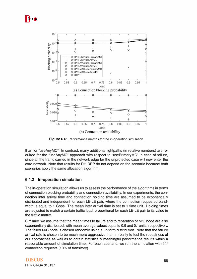
Fig. 4 shows the results for the two performance metrics for a single design scenario with 30 Tpbs of total offered traffic. The results for other traffic values are similar and omitted due to lack of space. The holding times are adjusted to match certain loads values (or fractions of 30 Tbps).

(a) Connection blocking probability

(b) Connection availability

Fig. 4. Performance metrics for the in-operation simulation.

Fig. 4a represents the blocking probability. As can be seen, the DH-DPP algorithm performs the poorest. This is greatly due to the fact that a connection cannot be allocated unless two active node-disjoint lightpaths are found (see Section IV.A.1), which is always the case when an M/C home node fails. The DH-PR-UNP and DH-PR-AVG approaches also obtain high blocking probability. Interestingly, the blocking probability of DH-PR-MAX approach is relatively poor when it is combined with “usePrimaryMC”, but improves drastically when the “useAnyMC” strategy is applied, remaining below 10-4 for all considered loads. Note that the gap between the “usePrimaryMC” and “useAnyMC” strategies stems from the allocation algorithm definitions (see Section IV.B.1). Namely, while “useAnyMC” considers up to 4 possible combinations for the primary path, the “usePrimaryMC” case enforces the usage of primary M/C home nodes for the primary path and blocks the connections otherwise.

Fig. 4b shows the average connection availability. Apart from DH-DPP, which guarantees 100% availability in the considered single-node failure scenario, DH-PR-MAX achieves more than six-nine availability at any load, indicating that the suitable degree of overdimensioning has been found. Interestingly, unavailability in the case of “useAnyMC” is higher than in “usePrimaryMC”. This can be explained by the fact that the higher the number of active connections (see Fig. 4a) implies lower spare capacity to reroute traffic in case of failure. Again, performance of DH-PR-UNP and DH-PR-AVG is poor even at low loads, which can be expected considering their low number of allocated transponders.

VII. CONCLUSIONS In this work, we present our preliminary results on the

dimensioning of metro/core networks with dual-homed access under the assumption of single metro/core node failure scenario. Our results show that equipping each M/C node with just enough transponders to recover from the most-damaging M/C node failure scenario and applying path restoration, we are capable of obtaining almost the same availability performance at a significantly reduced cost (up to 35% less transponders) than with dedicated path protection. Our future work will extend this preliminary assessment to other topologies and traffic patterns and to a disaster-aware scenario where multiple failures can happen simultaneously.

REFERENCES [1] M. Ruffini, et al., “DISCUS: An End-to-End Solution for Ubiquitous

Broadband Optical Access,” IEEE Communications Magazine, vol. 52, no. 2, pp. 24-32, February 2014.

[2] A. J. Phillips, et al., “Redundancy Strategies for a High Splitting Optically Amplified Passive Optical Network,” IEEE/OSA Journal of

Lightwave Technology, vol. 19, no. 2, February 2001. [3] A. Nag, D. B. Payne, and M. Ruffini, “N:1 Protection Design for

Minimising OLTs in Resilient Dual-Homed Long-Reach Passive Optical Network,” in Proc. of OFC 2014, San Francisco (USA), March 2014.

[4] S. Abeywickrama, M. Furdek, P. Monti, L. Wosinska, A. Nag, and E. Wong, “Dual-Homing Based Protection for Enhanced Network Availability and Resource Efficiency,” in Proc. of ACP2014, Shangai (China), November 2014.

[5] P. Pavon-Marino and J.-L. Izquierdo-Zaragoza, “Net2Plan: An open-source network planning tool for bridging the gap between academia and industry,” IEEE Network Magazine, in press.

[6] Net2Plan – The open-source network planner [Online]. Available: http://www.net2plan.com [Last accessed: January 1, 2015]

[7] J. Wang, V. M. Vokkarane, R. Jothi, X. Qi, B. Raghavachari and J. P. Jue, “Dual-Homing Protection in IP-Over-WDM Networks,” IEEE/OSA

Journal of Lightwave Technology, vol. 23, no. 10, pp. 3111-3124, October 2005.

[8] J. W. Suurballe, “Disjoint paths in a network,” Networks, vol. 4, no. 2, pp. 125-145, 1974.

[9] R. Andersen, F. Chung, A. Sen, and G. Xue, “On Disjoint Path Pairs with Wavelength Continuity Constraint in WDM Networks,” in Proc. of

INFOCOM2004, Hong Kong (China), March 2004. [10] S. Yuan and J. P. Jue, “Dynamic Lightpath Protection in WDM Mesh

Networks under Wavelength Continuity Constraint,” in Proc. of

GLOBECOM2004, Dallas (USA), December 2004. [11] J. P. Vasseur, M. Pickavet, and P. Demeester, Network Recovery:

Protection and Restoration, SONET-SDH, IP, and MPLS, Morgan Kaufmann, 2004.

[12] J. L. Izquierdo Zaragoza and P. Pavon-Marino, “Assessing IP vs optical restoration using the open-source Net2Plan tool,” in Proc. of

NETWORKS2014, Madeira (Portugal), September 2014. [13] J. M. Simmons, Optical Network Design and Planning, 2nd ed.,

Springer, 2014. [14] R. W. Sinnott, “Virtues of the Haversine,” Sky and Telescope, vol. 68,

no. 2, p. 159, 1984.

Figure 6.6: Performance metrics for the in-operation simulation.

than for “useAnyMC”. In contrast, many additional lightpaths (in relative numbers) are re-quired for the “useAnyMC” approach with respect to “usePrimaryMC” in case of failure,since all the traffic carried in the network edge for the unprotected case will now enter thecore network. Note that results for DH-DPP do not depend on the scenario because bothscenarios apply the same allocation algorithm.

6.4.2 In-operation simulation

The in-operation simulation allows us to assess the performance of the algorithms in termsof connection blocking probability and connection availability. In our experiments, the con-nection inter arrival time and connection holding time are assumed to be exponentiallydistributed and independent for each LE-LE pair, where the connection requested band-width is equal to 1 Gbps. The mean inter arrival time is set to 1 time unit. Holding timesare adjusted to match a certain traffic load, proportional for each LE-LE pair to its value inthe traffic matrix.

Similarly, we assume that the mean times to failure and to reparation of M/C node are alsoexponentially distributed, with mean average values equal to 0.9 and 0.1units, respectively.The failed M/C node is chosen randomly using a uniform distribution. Note that the failurearrival rate is chosen to be much more aggressive than in reality to test the robustness ofour approaches as well as to obtain statistically meaningful performance results within areasonable amount of simulation time. For each scenario, we run the simulation with 108

connection requests (10% of transitory).

FP7-ICT-GA 31813788

Figure 6.6 shows the results for the two performance metrics for a single design scenariowith 30 Tbps of total offered traffic. The results for other traffic values are similar andomitted due to lack of space. The holding times are adjusted to match certain loads values(or fractions of 30 Tbps).

Fig. 6.6a represents the blocking probability. As can be seen, the DH-DPP algorithm per-forms the poorest. This is due to the fact that a connection cannot be allocated unless twoactive node-disjoint lightpaths are found. The DH-PR-UNP and DH-PR-AVG approachesalso obtain high blocking probability. Interestingly, the blocking probability of DH-PR-MAXapproach is relatively poor when it is combined with “usePrimaryMC”, but improves dras-tically when the “useAnyMC” strategy is applied, remaining below 10�4 for all consideredloads. Note that the gap between the “usePrimaryMC” and “useAnyMC” strategies stemsfrom the allocation algorithm definitions. Namely, while “useAnyMC” considers up to 4possible combinations for the primary path, the “usePrimaryMC” case enforces the usageof primary M/C home nodes for the primary path and blocks the connections otherwise.

Fig. 6.6b shows the average connection availability. Apart from DH-DPP, which guarantees100% availability in the considered single-node failure scenario, DH-PR-MAX achievesmore than six-nine availability at any load, indicating that the suitable degree of overdi-mensioning has been found. Interestingly, unavailability in the case of “useAnyMC” ishigher than in “usePrimaryMC”. This can be explained by the fact that the higher the num-ber of active connections (Fig. 6.6a) implies lower spare capacity to reroute traffic in caseof failure. Again, performance of DH-PR-UNP and DH-PR-AVG is poor even at low loads,which can be expected considering their low number of allocated transponders.

6.5 Conclusions

In this work, we present a study on the dimensioning of metro/core networks with dual-homed access under the assumption of single metro/core node failure scenario. Our re-sults show that by equipping each M/C node with just enough transponders to recoverfrom the most-damaging M/C node failure scenario and by applying path restoration, it ispossible to obtain almost the same availability performance of dedicated path protectionbut at a significantly reduced cost (up to 35% less transponders).

FP7-ICT-GA 31813789

Chapter 7

Impact of Energy-Efficient Techniques on a DeviceLifetime

Telecom operators became particularly interested in energy-efficient techniques, sincethey see green ICT as a possible way to reduce their electricity bill. Looking at backbonenetworks, the active network elements consume a non-negligible amount of energy [91].This is due to the fact that they have to handle a huge amount of traffic. This requireshigh-capacity devices which are constantly powered on a 24-hour basis. Moreover, thetraffic exchanged by users will continuously increase in the forthcoming years, due to thepenetration of Internet connectivity as well as the multitude of smart devices coupled withbandwidth-intensive services. As a result, the power consumption of backbone networks isexpected to continue growing [52], unless proper counter measures are taken into account.

To this end, different energy-efficient approaches have been proposed in the literature, tar-geting both design and dynamic operations of backbone networks (see [28, 38] for detailedsurveys). Focusing on optical backbone networks, the majority of the energy-efficient al-gorithms are based on putting optical devices (e.g., transponders, regenerators, Reconfig-urable Optical Add/Drop Multiplexer (ROADMs), and Erbium Doped Fiber Amplifiers (ED-FAs)) into an energy-efficient mode (e.g., sleep mode) to reduce their power consumption.However, a possible drawback of this approach is that frequent on/sleep switching maynegatively impact the failure rate performance of a device, and consequently increase itsreparation costs [29, 30, 94]. This aspect cannot be neglected when considering the over-all benefits of a green strategy. In particular, it is important to make sure that the potentialsavings brought by a reduced power consumption level are not lower than the possibleextra reparation costs caused by a reduced lifetime. The work presented in Deliverable7.1 [9] pointed out this aspect and assessed different types of active components with themaximum allowable failure rate increase due to setting them into sleep mode on a regularbasis to save energy.

Leveraging these previous works, the aim of the work presented in this chapter is to pro-vide answers to the following questions: (i) what are the main sleep mode and hardware(HW) parameters that influence the failure rate performance of EDFAs in optical backbonenetworks?, and (ii) under which conditions may the lifetime of an EDFA increase as a re-sult of being set into sleep mode? The material presented in the chapter is organized asfollows. We first present the main causes that impact the EDFA lifetime. Then, a failurerate acceleration factor model is presented in order to understand the role of both sleepmode and HW parameters in the potential changes of the failure rate of an EDFA . Themodel is then evaluated by considering energy-efficient schemes that are based on puttingthe EDFA into sleep mode. In particular, the section considers an energy-efficient RWAalgorithm, where the main idea is to route the traffic over already used fiber links. In thisway it is possible to maximize the number of EDFAs that can be set into sleep mode andtherefore save energy.

FP7-ICT-GA 31813790

7.1 Impact of Sleep Mode Operations on a Device Lifetime

This section provides a general overview of the physical phenomena that may impact thelifetime of a network device put into sleep mode in order to save energy.

Transitions between on and sleep states affect the conditions in which a device operates,in particular its temperature [25]. There are several models that describe how temperatureimpacts the lifetime of a device. One of them is the Arrhenius law [24], which defines interms of an acceleration factor how much the lifetime of a device could increase/decreaseif operated at a temperature different from a reference one. More formally, the accelerationfactor derived from the Arrhenius law can be expressed as:

AF T1 =�T1

�Tr= e

�EaK (

1T1

� 1Tr ) (7.1)

where Ea is the activation energy, K is the Boltzmann constant, and �T1 and �Tr are thefailure rate at the operating T

1

and reference Tr temperatures, respectively. If the effectsof the Arrhenius law were the only phenomenon to consider, an energy-efficient schemewould have a positive impact on the lifetime of a device, as the operating temperature ofa device in sleep mode is typically lower than in normal working conditions (i.e., when adevice is powered on).

However, there are also other physical phenomena that need to be considered, whichmight negatively impact the lifetime of a device. For example, it is well known that temper-ature changes may affect differently the expansion of different materials within the samecomponent due to different Coefficients of Temperature expansion (CTEs). In turn, thedevice may suffer strain and fatigue when temperature conditions change, in particularwhen this happens in a cyclic way. This phenomenon can be observed for many electronicdevices, in particular in solder junctions. The Coffin-Manson model [34, 63] describes theeffects of material fatigue caused by cyclic thermal stress and it is used to predict the num-ber of temperature cycles that a component can endure before failing. More formally, thenumber of cycles to failure can be expressed by the following equation [35, 55]:

Nf = C0

(�T ��T0)�q (7.2)

where �T is the temperature variation, �T0 is the maximum temperature variation thatcan be afforded without an impact on the failure rate, C

0

is a material dependent constant,and q is the Coffin-Manson exponent. Then using Eq. (7.2), the failure rate due to thermalcycling can be defined as:

��T =fTC

Nf(7.3)

where fTC is the frequency of thermal cycling and ��T is the estimated failure rate. Thevalue of fTC can be obtained via experimental measures. In this case, both the frequencyof temperature changes and the temperature variation play an important role. It is becausethe more often a device experiences a temperature gradient (i.e., as a result of being putinto sleep mode), the shorter its lifetime might be. There are other models available inthe literature (e.g., Engelmeier [43], Norris-Lanzberg [70]) that introduce additional factors(e.g., solder dimensions, chemical characteristics, dwell time) into a lifetime predictionmodel. On the other hand, they all share their dependence on the temperature variationand frequency of the temperature cycles.

FP7-ICT-GA 31813791

One could argue that on/sleep switching (i.e., power cycling) based schemes produce alocalized and internally induced heating in the device (Joule heating) so that the resultingtemperature variation may not be uniformly distributed over the whole device as it happenswith thermal cycling, where the device heating is externally induced. On the other hand,the work in [78] and [76] confirms that the fast local temperature changes caused by powercycling (that can be up to 100 times faster [23] than the thermal cycling) also negativelyimpact the lifetime of a device. From the consideration above it can be concluded thattemperature and the temperature variations are relevant phenomena that might impact thelifetime of a device.

When looking at optical backbone networks, the set of elements that may be the target ofan energy-efficient scheme include: transponders, regenerators, ROADMs, and EDFAs.Among these various elements, the EDFA is the one where the impact of the temperatureconditions and temperature variations is the most critical [94].

7.2 EDFA Failure Rate Model and Average Failure Rate Accel-eration Factor

This section focuses on modeling the lifetime variations of an EDFA as a function of itstemperature and temperature variations1.

Let us denote as Dijk the lifetime of the EDFA i placed on the fiber link from node j tonode k. Dijk is defined as the inverse of the EDFA failure rate �ijk:

Dijk =1

�ijk[h]. (7.4)

When an EDFA is in a low-power state (or sleep state), its temperature is reduced com-pared to the full-power state. According to the Arrhenius law, Eq. (7.1), this induces adecrease in the failure rate compared to the full power state. The failure rate �on�sleep

ijk ofEDFA i implementing sleep mode capabilities and placed on the fiber link between node jand node k is:

�on�sleepijk =

h(1� ⌧ sleepijk )�onijk + ⌧ sleepijk �sleepijk

i[1/h], (7.5)

where, �sleepijk is the failure rate when EDFA i is in sleep mode, �onijk is the failure rate at fullpower, and ⌧ sleepijk 2 [0, 1] is the normalized time in which EDFA i is in sleep mode (if equalto 1 the EDFA i is always in sleep mode). Thus, the overall failure rate is the averagedsum of the failure rates at full power and in sleep mode. The first consideration is that thelonger the EDFA is in sleep mode, the higher the reduction in the failure rate. However, asreported in Eqs. (7.2) and (7.3), also the interval in which the temperature varies (i.e., �T )and the frequency of thermal cycling (i.e., fTC in [cycle/h]) impacts the failure rate. Let usdefine �trijk as the failure rate of the device when a temperature variation occurs. FollowingEq. (7.3), �trijk can be defined as:

�trijk =f trijk

Nfijk

[1/h], (7.6)

1The model is general enough that can be extended to model the failure rate and the failure rate variationsof any other network device.

FP7-ICT-GA 31813792

where f trijk is the on/sleep frequency and Nf

ijk is the number of cycles to failure. FromEq. (7.6) it can be seen that as the power switching frequency is reduced, the failure rate�trijk is also reduced. Moreover, Nf

ijk is a technological parameter that depends on thespecific HW used to assembly the EDFA.

In order to put together both the effects of Eq. (7.6) and Eq. (7.5), we assume that �on�sleepijk

and �trijk are statistically independent [27] and their effects are additive [35]. In this way,the overall failure rate �ijk is the sum of the individual failure rates:

�ijk = �on�sleepijk + �trijk[1/h]. (7.7)

Since we are interested in evaluating in which way the sleep mode may impact the lifetimeof an EDFA, we define a failure rate acceleration factor, i.e., AFijk, similar in concept tothe one defined by the Arrhenius law, i.e., Eq. (7.1). The acceleration factor is a metric thatmeasures the increase of the failure rate with respect to a reference temperature. In orderto model the value of AFijk, we first define the failure rate acceleration factor of an EDFAin sleep mode as:

AF sleepijk =

�sleepijk

�onijk, (7.8)

which is always lower than one. This term can be computed from using the Arrhenius lawgiven the difference in the operating temperature of the device and its activation energy.Moreover, we introduce the parameter �ijk:

�ijk =1

�onijkNfijk

[h/cycle], (7.9)

which is defined as the inverse of the failure rate at full power multiplied by the numberof cycles to failure. Both terms are fixed and can be measured on the device when sleepmodes are not applied. Finally, the overall failure rate acceleration factor of an EDFA canbe defined as:

AFijk =�ijk�onijk

= 1� (1�AF sleepijk )⌧ sleepijk + �ijkf

trijk. (7.10)

The acceleration factor AFijk comprises two terms: the first one is (1 � AF sleepijk )⌧ sleepijk

which tends to decrease the AFijk value, and the second one �ijkf trijk which has the oppo-

site effect. Moreover, AFijk is influenced by two types of parameters: technological (i.e.,AF sleep

ijk and �ijk) which are strictly related to the HW used to build the EDFA, and sleep-mode-related (i.e., ⌧ sleepijk and f tr

ijk) which instead depend on the energy-efficient algorithmused.

When, in a given network, a number of EDFAs are put into sleep mode in order to save en-ergy (with on/sleep switching frequencies and sleep periods that might not be necessarilythe same for each one of them), it is important to model their overall performance in termsof failure rate acceleration factor. We define the following metric for this purpose:

AF =

Pijk AFijk

I. (7.11)

The AF in Eq. (7.11) defines the average EDFA failure rate acceleration factor, where I isthe total number of EDFAs deployed in the network. If AF > 1, it can be expected that,on average, the EDFAs in the network will fail more frequently than in normal operating

FP7-ICT-GA 31813793

conditions (i.e., when a green strategy is not used). If AF = 1, the average failure rate ofEDFAs will not change, and if AF < 1 it can be expected that, on average, the EDFAs inthe network will fail less frequently. It should be noticed that AF is not the only metric thatcan be used. The choice is up to the network operator that might focus also on a differentmetric, e.g., on the EDFA with the worst failure rate acceleration performance.

7.3 Case Study

This section presents a case study where a green strategy putting EDFAs into sleep modeis applied to a specific optical backbone network under a dynamic lightpath provisioningscenario. We first explain how the green algorithm works, and then present an analysis ofthe various parameters impacting the average EDFA failure rate acceleration factor value

7.3.1 Green Strategy and Simulation Scenario

This simulation study is based on a green RWA strategy called Weighted Power AwareLightpath Routing (WPA-LR) [93] tested on the COST239 optical backbone network. Theprovisioning scenario considers dynamic traffic where each connection request is assumedto require a full wavelength capacity.

The WPA-LR algorithm works in the following way. A separate network connectivity graphis considered for each wavelength, i.e., a wavelength plane approach is utilized. If a givenwavelength is already used on a fiber link to provision a lightpath, the fiber link will notappear on that specific wavelength plane. For an incoming connection request the pathat minimum cost (if any) is computed on each wavelength plane. The path that has theoverall minimum cost (among the ones found on each wavelength plane) is then chosenas the route for the connection request. If no path can be found on any wavelength plane,the connection is rejected. Under the assumption that the only devices that are put intosleep mode (in order to save energy) are the EDFAs (i.e., the other network componentssuch as transceivers, ROADMs, or higher layer electronics are considered to be alwayson), the cost function used in the WPA-LR algorithm works as follows. If a fiber link isnot in use, its cost is equal to the power necessary to operate all the EDFAs deployedalong its length (i.e., the fiber link power consumption cost). If a fiber link is in use, itsrouting cost becomes the product of its power consumption cost and a parameter ↵ thatvaries in the range (0;1]. Values of ↵ close to 0, encourages WPA-LR to select routes atminimum power cost, while with 0 < ↵ < 1 WPA-LR tends to make routing choices that area compromise between power consumption minimization and (fiber) resource efficiencymaximization. When ↵ = 1, the WPA-LR behaves in the same way as a conventionalshortest path (SP) approach, where still some energy savings can be achieved becausethe EDFAs that are not used can be set into sleep mode. More details about the WPA-LRstrategy are available in [93].

In the simulation work on the COST239 network topology it is assumed that each fiberlink comprises two unidirectional fibers each one carrying 16 wavelengths. It is assumedthat wavelength conversion is not available. Connection requests are bidirectional andtheir source and destination pairs are uniformly chosen among the network nodes. Theyarrive according to a Poisson process while the service time for each connection request isexponentially distributed with an average holding time equal to 6 hours. EDFAs are placed

FP7-ICT-GA 31813794

0 100 200 300 400 50010

20

30

40

50

60

70

80

90

100

Load [Erlang]

Ave

rag

e N

orm

aliz

ed

Tim

e in

Act

ive

Sta

te [

%]

α=1 (SP)

α = 0.75

α = 0.5

α = 0.25

α ≈ 0

0 100 200 300 400 5000

0.2

0.4

0.6

0.8

1

1.2

1.4

Load [Erlang]

Ave

rag

e O

n/S

lee

p F

req

ue

ncy

[cy

cle

s/d

ay]

α=1 (SP)

α = 0.75

α = 0.5

α = 0.25

α ≈ 0

Figure 7.1: Average normalized time in percentage an EDFA is in active state (left), andaverage EDFA on/sleep frequency (right) as a function of the network load.

every 80 km and the power consumed by an EDFA in sleep mode is assumed to be 20%of the power when fully operational.In the case study the traffic load is varied from 10 to 420 Erlang. These values are chosenin order to investigate different conditions where the network blocking probability does notexceed 10%. In order to measure the value of the average EDFA failure rate accelerationfactor (i.e., AF as defined in equation 7.11), it is assumed that all the EDFAs deployedin the network have the same HW characteristics, while the value of the frequency andthe duration of each sleep cycles are collected by simulating the WPA-LR algorithm fordifferent values of ↵. Simulation results are averaged over a series of 10 experiments with105 connection requests in each experiment.

7.3.2 Impact of Traffic Load on the Sleep Mode Duration and the On/SleepFrequency

Fig. 7.1 reports the average normalized time in active state (left) and the on/sleep fre-quency (right) for the EDFAs in the network as a function of the load. Results are pre-sented for different values of the parameter ↵. Several considerations hold in this case.First, the average normalized time in active state tends to increase with increasing loadvalues (as expected), since more EDFAs need to be powered on in order to meet the traf-fic requirements. Moreover, for load higher than 350 Erlang the average normalized time inactive state is nearly equal to 100%, meaning that all the EDFAs in the network are alwayspowered on. Second, the average on/sleep frequency tends to decrease with increasingload. However, the maximum value of the on/sleep frequency does not always occur at theminimum value of load. This is due to the fact that some of the EDFAs are always in sleepmode when traffic is very low. Third, the parameter ↵ has a strong impact on the results. Inparticular, when the algorithm tends to exploit short paths (↵ = 1) the average normalizedtime in active state is higher compared to a pure power minimization approach, i.e., ↵ = 0,and the average on/sleep frequency is almost one order of magnitude higher since EDFAsfrequently change their power state.

7.3.3 Average EDFA Failure Rate Acceleration Factor

Fig. 7.2 reports a number of level curves representing the average EDFA failure rate ac-celeration factor (AF ) (equation 7.11) as a function of the value of AF sleep defined as

FP7-ICT-GA 31813795

0 1 2 3 4 50

0.1

0.2

0.3

0.4

0.5

0.6

0.7

0.8

0.9

1

χ [h/cycle]

AF

sle

ep

0.7

0.8

0.9

1

1.1

1.2

1.3

1.4

1.5

1.6

AF

Figure 7.2: Average EDFA failure rate acceleration factor (AF ) as a function of AF sleep and�, with ↵ = 0.5 and a load of 150 Erlang.

(P

ijk AFsleepijk )/I, and � defined as (

Pijk �ijk)/I. The results are obtained with ↵ = 0.5 at

load equal to 150 Erlang.

The red dashed line highlights the level curve AF = 1. The region on the left of thiscrossover line represents the zone where on average EDFAs in the network fail less oftenwhen compared to the case in which the WPA-LR algorithm is not used, i.e., AF < 1.On the contrary, the region on the right is the zone in which AF > 1, i.e., EDFAs onaverage are expected to fail more often when compared to the case in which the WPA-LR algorithm is not used. From the figure, it can be noticed that both AF sleep and � playa crucial role in determining the effectiveness of an energy-efficient strategy in terms ofaverage EDFA failure rate increase/decrease. In particular, AF sleep is influenced by thedecrease of temperature on the device, which is expected to happen when EDFAs are insleep mode. On the other hand � becomes the discriminating factor, meaning that deviceswhose � is very high (in this case higher than 2.7 h/cycle) will experience on average anincrease of their failure rate.

Fig. 7.3, on the other hand, considers the impact of the parameter ↵ on the position of thevalue for AF = 1. The traffic load is equal to 150 Erlang, which corresponds to mediumtraffic conditions. It is interesting to notice that as the algorithm tends to target the powerminimization (low values of ↵), the region in which AF < 1 is increased. This is mainlydue to the fact that, as shown in Fig. 7.1, with decreasing values of ↵ EDFAs on averagespend more time in sleep mode and the average value of their on/sleep transitions is alsolower.

7.3.4 Impact of the HW parameters

The left part of Fig. 7.4 reports the different values of � (i.e., (P

ijk �ijk)/I), that are re-quired to have AF = 1. The value of � is presented as a function of the traffic load and fordifferent values of AF sleep (i.e., (

Pijk AF sleep

ijk )/I). The algorithm parameter ↵ is set to 0.5.

Note that the areas below each curve represent values of � for which AF < 1. For lowvalues of load � is very small, i.e., � < 1 [h/cycle]. This is due to the fact that the averagefrequency of on/sleep transitions is relatively high as shown in Fig. 7.1. This means that

FP7-ICT-GA 31813796

0 2 4 6 80

0.2

0.4

0.6

0.8

1

χ [h/cycle]

AFsl

eep

α=1 (SP)α = 0.75α = 0.5α = 0.25α ≈ 0

Figure 7.3: Level curves for AF = 1 for different values of ↵ with a load of 150 Erlang.

50 100 150 200 250 300 350 4000

1

2

3

4

5

6

7

Load [Erlang]

χ [

h/c

ycle

]

AFsleep=0.8

AFsleep=0.5

AFsleep=0.2

50 100 150 200 250 300 350 4000.5

1

1.5

Load [Erlang]

AF

Lower Bound

χ=0.1

χ=0.5

χ=0.9

χ=1.5

Figure 7.4: Values of � required to have AF = 1 with ↵ = 0.5 (left), and AF with AF sleep =0.5 and ↵ = 0.5 (right), both as a function of the load.

even if a device is equipped with better hardware capabilities to limit the thermal cyclingeffect, high average on/sleep frequency may still negatively impact the value of AF . How-ever, for intermediate values of load (between 20 and 125 Erlang), the frequency of cyclespromptly decreases, allowing higher values for �, i.e., up to a max of 5.5 [h/cycle], whilestill ensuring favorable conditions in terms of EDFAs average failure rate acceleration fac-tor, i.e., AF < 1. For high traffic values, the average normalized time EDFAs spend inactive state is almost 100%, setting the value of AF to be greater than 1 even for verysmall values of �. Finally, it can be observed that the trend does not change with differentvalues of AF sleep (even though the absolute values are different).

The right part of Fig. 7.4 presents values of AF for different values of the traffic load and �when ↵ = 0.5 and AF sleep = 0.5. The figure reports also a lower bound, which correspondsto the case of � = 0, i.e., no thermal cycling effect. Two considerations hold in this case.First, for increasing values of the traffic load, AF converges to one, which corresponds tothe situation in which all devices are always powered on, and therefore the average EDFAfailure rate acceleration factor AF remains unchanged. Second, it can be seen that when� is increasing, the region in which the AF < 1 is reduced. However, the effect is mitigatedfor intermediate values of load, meaning that there is a tradeoff between power efficiencyand the value of the average failure rate acceleration factor.

FP7-ICT-GA 31813797

7.4 Conclusions

The chapter considered the impact that energy-efficient techniques have on the compo-nent lifetime in an optical backbone network. The focus was on understanding the effectsof putting EDFAs into sleep mode. We have developed a simple model, showing thatthe EDFA failure rate variations are influenced by the traffic, the energy-aware algorithmparameters, the time spent in sleep mode, the frequency of on/sleep cycles, and the char-acteristics of the EDFA HW. The chapter showed that frequent on/sleep transitions mayhave a negative impact on the EDFA failure rate. However, this work is a first step towardsa more comprehensive approach, since there might be conditions under which the failurerate of a component may benefit from long (and not frequent) sleep periods. As next stepsit will be worth to consider the influence of various traffic patterns (including bursty traffic),and to investigate energy-efficient algorithms targeting explicitly the increase of lifetime foroptical networks.

FP7-ICT-GA 31813798

Chapter 8

Control plane interaction for resilience scenarios

The end-to-end optical transport networks where DISCUS control plane architecture isinvolved moves huge volumes of data from one point to another in geographically differentlocations. It is not uncommon a failure in a fiber links or some component in a DISCUSnode. The source of the failures is related to failure of equipment in a link (e.g., amplifiers),cuts in the fibers, e.g., because of roadworks , digging, power failure or bad weather. FCCreports publish findings that long haul networks experience annually 3 cuts for 1500 kmsof fiber. Internal operator data reports even higher fiber cut failure in areas with numerousroadworks. FCC data implies a cut every four days in a typical long haul network with45000 km of fiber. Thus, it is necessary to provide the network means of maintaining theservice continuity in the presence of failures. Not only should the network be able to reactto a single failure, but also to a multiple failure situation in which several link or nodesare affected simultaneously (or one after the other). In this chapter, the relation betweenthe DISCUS control plane and network survivability is analyzed. First the control planearchitecture and its main components that interact in case of failure are presented. Next, acomparative between the traditional distributed control plane approach and the centralizedSDN approach is presented. Next, a use case is analyzed. Finally, a study shows which isthe optimal location of a DISCUS core network controller to minimize the restoration time.

8.1 DISCUS control plane architecture

Considering the architecture of the MC node, as defined in Deliverable D6.1, it is possibleto identify three main logical component for the network control plane : the access networkcontroller, in charge of controlling the access network elements; the core network con-troller, in charge of controlling the elements carrying out core transmission; the networkorchestrator, in charge of taking requests from the SP and translating them into high-levelcommands for the access and core network controllers.

The network orchestrator is defined as a parent controller or a centralized “controller ofcontrollers”. It handles the automation of end-to-end connectivity provisioning, working ata higher, abstracted level and covering inter-domain aspects between the access and themetro/core network. Its functionalities are the following: The access network controller isin charge of controlling the access network elements, while the core controller is in chargeof receiving commands from the network orchestrator and transforming them in the D-CPIfor the metro/core network. For the core network controller, the technologies that are inthe underlying network are Wavelength Switched Optical Network / Spectrum SwitchedOptical Network (WSON/SSON) which are based on the GMPLS distributed control plane.

As it can be seen in the previous definition of the entities, some feedback from the networkis required for failure scenarios. The following section compares the resilience mecha-nisms in centralized and distributed scenarios.

FP7-ICT-GA 31813799

8.2 Centralised vs. distributed resilience mechanism

8.2.1 Distributed control plane approach for failure scenarios

When the functions of the control plane are co-located with the nodes and do no rely on acentralized controller, they need to interact with each other in a distributed way in order torecover from network failures. Pure distributed GMPLS is an example of such distributedapproach. The main concept in a distributed control plane is that the owner of a service(e.g. LSP, lambda, etc.) is the responsible of initiating any survivability actions. The mainresilience mechanisms are protection and restoration. In the case of protection, when theelement in control of the service detects a problem in the main path, the service is au-tomatically switched to the backup path. Resources for both main and backup paths arealways reserved, and thus, there is a huge resource consumption. The main benefit isthe sub-50 ms recovery time that can be achieved with protection. The other main re-silience mechanism is restoration. In this case, the nodes adjacent to the elements thathave failed (in the case of a fiber cut, the switching nodes adjacent to the fiber) notify viarouting protocol the failure. Then, the routing protocols keeps on disseminating the newstate of the network, and all nodes become aware of the existing resource failed. Also,a second mechanism is used to speed up the recovery. The signaling mechanism (e.g.RSVP-TE in distributed GMPLS) maintains state in all the nodes of the path. When afailure happens, and the adjacent nodes become aware of the failure, using the signalingprotocol, the source node (owner of the service) is notified. Then, each node that ownsservices that have failed recomputed a new path. Note that for the new compute path tobe accurate, either the routing protocol has informed about the exact failure, or the sig-naling protocol carries information about the exact location of the failure. The restorationprocedure takes longer that the protection, but is able to adapt to changing network cir-cumstances, but cannot achieve an optimal resource usage after the failure, as all pathcomputation recoveries are performed un-coordinately. Finally, restoration in a distributedcontrol plane suffers the problem of piggybacking. As mentioned previously, when thereis a failure all nodes that own a service that uses the failed element are notified. At thatpoint, all of them compute their backup path. It may be entirely possible that the pathsresulting from these almost concurrent computations share resources (e.g. a lambda insome path). This will trigger a race between signaling sessions. The fastest one gets theresource, while the following ones, need to piggyback and compute again the path. Thissecond computation is not done immediately, but a random time is left, to avoid concurringagain in a computation. The problem of piggybacking can lead to high restoration timeswhen the network is highly utilized. A centralized approach for the computation can solvethe problems of the distributed control plane.In spite of the problems of the recovery of a distributed control plane, it is a very robustscheme, as it can survive many failure scenarios (including controllers).Figure 8.1 shows the message exchange between nodes in the control plane. Let’s as-sume there is a path from N

0

to N3

. When there is a failure at a node, for instance N2

,this node sends an RSVP Error message to the head-end node (in this case N

0

). Oncethe head-end node receives the failure notification, it computes a new path avoiding thisfailed node and establishes a new connection. This is done using the RSVP Path-Resvmessage exchange, as shown in Figure 8.1 .The restoration in a distributed control plane suffers the problem of piggybacking. As men-tioned previously, when there is a failure all nodes that own a service that uses the failed

FP7-ICT-GA 318137100

! !!

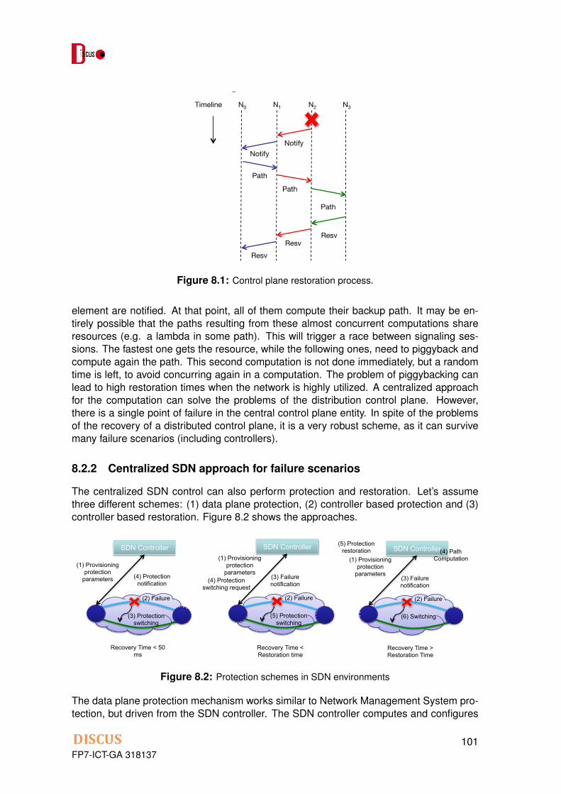
FP7!–!ICT!–!GA!318137! 10!DISCUS!!!

adapt! to! changing! network! circumstances,! but! cannot! achieve! an! optimal! resource!usage! after! the! failure,! as! all! path! computation! recoveries! are! performed! un\coordinately.!Figure! 1\2! shows! the!message! exchange! between! nodes! in! the! control! plane.! ! Let’s!assume!there!is!a!path!from!N0!to!N3.!When!there!is!a!failure!at!a!node,!for!instance!N2,!this!node!sends!an!RSVP!Error!message!to!the!head\end!node!(in!this!case!N0).!Once!the!head\end!node! receives! the! failure! notification,! it! computes! a! new!path! avoiding! this!failed!node!and!establishes! a!new!connection.!This! is!done!using! the!RSVP!Path\Resv!message!exchange,!as!shown!in!Figure!1\2.!

!Figure 1-2 Control plane restoration process

The!restoration!in!a!distributed!control!plane!suffers!the!problem!of!piggybacking.!As!mentioned!previously,!when!there!is!a!failure!all!nodes!that!own!a!service!that!uses!the!failed!element!are!notified.!At!that!point,!all!of!them!compute!their!backup!path.!It!may!be!entirely!possible!that!the!paths!resulting!from!these!almost!concurrent!computations!share!resources!(e.g.!a!lambda!in!some!path).!This!will!trigger!a!race!between!signaling!sessions.!The!fastest!one!gets!the!resource,!while!the!following!ones,!need!to!piggyback!and!compute!again!the!path.!This!second!computation!is!not!done!immediately,!but!a!random!time!is!left,!to!avoid!concurring!again!in!a!computation.!!The!problem!of!piggybacking-can!lead!to!high!restoration!times!when!the!network!is!highly!utilized.!A!centralized!approach!for!the!computation!can!solve!the!problems!of!the!distribution!control!plane.!However,!there!is!a!single!point!of!failure!in!the!central!control!plane!entity.!In!spite!of!the!problems!of!the!recovery!of!a!distributed!control!plane,!it!is!a!very!robust!scheme,!as!it!can!survive!many!failure!scenarios!(including!controllers).!

1.2.2 Centralized-SDN-approach-for-failure-scenarios-

The!centralized!SDN!control!can!also!perform!protection!and!restoration.!Let’s!assume!three!different!schemes:!(1)!data!plane!protection,!(2)!controller!based!protection!and!(3)!controller!based!restoration.!!The!data!plane!protection!mechanism!works!similar!to!Network!Management!System!protection,!but!driven!from!the!SDN!controller.!The!SDN!controller!computes!and!configures!a!working!and!a!protection!path,!which!are!instantiated!in!the!network!

N0 N1 N2 N3

Path

Path

Path

Resv

Timeline

Resv Resv

Notify Notify

Figure 8.1: Control plane restoration process.

element are notified. At that point, all of them compute their backup path. It may be en-tirely possible that the paths resulting from these almost concurrent computations shareresources (e.g. a lambda in some path). This will trigger a race between signaling ses-sions. The fastest one gets the resource, while the following ones, need to piggyback andcompute again the path. This second computation is not done immediately, but a randomtime is left, to avoid concurring again in a computation. The problem of piggybacking canlead to high restoration times when the network is highly utilized. A centralized approachfor the computation can solve the problems of the distribution control plane. However,there is a single point of failure in the central control plane entity. In spite of the problemsof the recovery of a distributed control plane, it is a very robust scheme, as it can survivemany failure scenarios (including controllers).

8.2.2 Centralized SDN approach for failure scenarios

The centralized SDN control can also perform protection and restoration. Let’s assumethree different schemes: (1) data plane protection, (2) controller based protection and (3)controller based restoration. Figure 8.2 shows the approaches.

! !!

FP7!–!ICT!–!GA!318137! 11!DISCUS!!!

elements.!When!there!is!a!failure,!the!network!elements!can!notify!the!controller,!which!can!configure!the!protection!path!to!recover!from!the!failure!in!the!network.!The!protection,!as!well!with!the!distributed!control!plane,!can!be!performed!by!the!data!plane!in!case!sub\50!ms!recovery!time!is!needed.!In!this!case,!the!control!plane!is!in!charge!only!of!computing!and!setting!up!the!working!and!protection!paths,!but!it!is!not!involved!at!failure!time.!

The!controller,!according!to!ITU\T1,!can!be!used!to!perform!a!controller\based!protection,!or!controller\based!restoration.!!

!Figure 1-3 Protection schemes in SDN environments

In!the!controller!based!protection,!SDN!controller!is!in!charge!of!provisioning!both!working!and!protection!path!and!instructs!the!data!plane!to!notify!the!controller!whenever!a!failure!happen.!When!the!failure!happens,!the!SDN!controller!commands!to!switch!to!the!protection!path.!This!mechanism!is!not!as!fast!as!the!data!plane!protection,!but!faster!than!a!restoration!as!it!does!not!need!to!compute!path.!The!advantage!is!that!it!lowers!the!data!plane!requirements.!

In!the!controller!based!restoration,!the!SDN!controller!is!notified!of!all!the!failures.!The!main!difference!with!the!distributed!case!is!that!the!SDN!controller!is!the!owner!of!all!the!services.!When!the!SDN!controller!receives!the!notification!of!the!failed!element,!it!will!look!in!its!database!and!see!how!many!services!are!affected!by!the!failure.!Then,!it!performs!the!computation!of!new!paths!for!all!the!services.!Such!computation!can!be!performed!in!a!single!computational!step,!which!allows!to!apply!optimization!techniques.!The!result!of!the!recovery!of!multiple!paths!via!SDN!controller!can!lead!to!a!very!high!restorability!degree,!and!an!optimal!use!of!resources.!Furthermore,!as!the!controller!centralizes!the!provisioning!and!computation,!no!piggybacking!is!needed.!All!paths!computed!by!the!SDN!controller!will!be!valid.!

The!main!problem!of!the!centralized!SDN!controller!approach!is!its!high!dependability!on!the!controller,!and!having!a!path!to!the!controller.!For!the!availability!of!the!controller,!dual\controller!approach!(service\backup)!is!recommended!for!deployments.!!

To!sum!up,!following!table!presents!a!comparison!between!the!different!controllers!approaches:!

!!!!!!!!!!!!!!!!!!!!!!!!!!!!!!!!!!!!!!!!!!!!!!!!!!!!!!!!1!ITU\T!meeting!Bundang,!South!Korea,!9!–13!Mar.!2015!“Controller!based!protection”!

SDN Controller

(1) Provisioning protection

parameters (4) Protection notification

(2) Failure

(3) Protection switching

Recovery Time < 50 ms

SDN Controller (1) Provisioning

protection parameters

(3) Failure notification

(2) Failure

(5) Protection switching

Recovery Time < Restoration time

(4) Protection switching request

SDN Controller (1) Provisioning

protection parameters

(3) Failure notification

(2) Failure

(6) Switching

Recovery Time > Restoration Time

(5) Protection restoration (4) Path

Computation

Figure 8.2: Protection schemes in SDN environments

The data plane protection mechanism works similar to Network Management System pro-tection, but driven from the SDN controller. The SDN controller computes and configures

FP7-ICT-GA 318137101

a working and a protection path, which are instantiated in the network elements. Whenthere is a failure, the network elements can notify the controller, which can configure theprotection path to recover from the failure in the network. The protection, as well with thedistributed control plane, can be performed by the data plane in case sub-50 ms recoverytime is needed. In this case, the control plane is in charge only of computing and settingup the working and protection paths, but it is not involved at failure time.

The controller, according to ITU-T [53], can be used to perform a controller-based protec-tion, or controller-based restoration.

In the controller based protection, SDN controller is in charge of provisioning both workingand protection path and instructs the data plane to notify the controller whenever a failurehappen. When the failure happens, the SDN controller commands to switch to the protec-tion path. This mechanism is not as fast as the data plane protection, but faster than arestoration as it does not need to compute path. The advantage is that it lowers the dataplane requirements.

In the controller based restoration, the SDN controller is notified of all the failures. Themain difference with the distributed case is that the SDN controller is the owner of all theservices. When the SDN controller receives the notification of the failed element, it will lookin its database and see how many services are affected by the failure. Then, it performsthe computation of new paths for all the services. Such computation can be performedin a single computational step, which allows to apply optimization techniques. The resultof the recovery of multiple paths via SDN controller can lead to a very high restorabilitydegree, and an optimal use of resources. Furthermore, as the controller centralizes theprovisioning and computation, no piggybacking is needed. All paths computed by the SDNcontroller will be valid.

The main problem of the centralized SDN controller approach is its high dependability onthe controller, and having a path to the controller. For the availability of the controller,dual-controller approach (service-backup) is recommended for deployments.

8.3 Impact of a centralized or distributed control plane in DIS-CUS

DISCUS defined use cases in D6.1. One of this scenarios is the PON protection with adual-homed N:1 OLT scheme. This scenario emulates the provisioning of a dedicated as-sured L1 service over PON, describing the interaction between ONU, OLT, node controller,and network control plane. We assume this service is a point-to-point service betweenany two points in the network. In order to understand the requirements on all interfacesinvolved we carry out an analysis of the upstream and downstream control messages re-quired. The interactions between the control plane elements is the following:

1. The fibre cut is identified by a fault management system that triggers an alarm.

2. The access controller in MC node 1 informs the network orchestrator about the fail-ure.

3. The orchestrator informs the core controller to setup the pre-calculated core backuppaths corresponding to the failure.

FP7-ICT-GA 318137102

4. The orchestrator then communicates to the access controller in the MC node hostingthe standby OLT, passing the information required to activate the OLT as well as theappropriate protection paths that need to be activated in the node.

5. In the meantime the core controller will configure the core nodes

6. The access controller will configure the access elements

7. The core controller will then provide feedback to the orchestrator.

8. The access controller of the standby node on the access protection.

Figure 8.3 presents graphically the steps just described in the reference architecture.

! !!

FP7!–!ICT!–!GA!318137! 11!DISCUS!!!

1.3 Use$case$example$for$resilience$mechanisms$

DISCUS!defined!use!cases!in!D6.1.!One!of!this!scenarios!is!the!PON!protection!with!a!dual[homed!N:1!OLT!scheme.!This!scenario!emulates!the!provisioning!of!a!dedicated!assured!L1!service!over!PON,!describing!the!interaction!between!ONU,!OLT,!node!controller,!and!network!control!plane.!We!assume!this!service!is!a!point[to[point!service!between!any!two!points!in!the!network.!In!order!to!understand!the!requirements!on!all!interfaces!involved!we!carry!out!an!analysis!of!the!upstream!and!downstream!control!messages!required.!The!interactions!between!the!control!plane!elements!is!the!following:!

1. The!fibre!cut!is!identified!by!a!fault!management!system!that!triggers!an!alarm.!!2. The!access!controller!in!MC!node!1!informs!the!network!orchestrator!about!the!

failure.!!3. The!orchestrator!informs!the!core!controller!to!setup!the!pre[calculated!core!

backup!paths!corresponding!to!the!failure.!!4. The!orchestrator!then!communicates!to!the!access!controller!in!the!MC!node!

hosting!the!standby!OLT,!passing!the!information!required!to!activate!the!OLT!as!well!as!the!appropriate!protection!paths!that!need!to!be!activated!in!the!node.!

5. In!the!meantime!the!core!controller!will!configure!the!core!nodes!!6. The!access!controller!will!configure!the!access!elements!!7. The!core!controller!will!then!provide!feedback!to!the!orchestrator.!8. The!access!controller!of!the!standby!node!on!the!access!protection.!!

Next!figure!presents!the!graphically!previous!steps!in!the!reference!architecture.!!

!Figure 1-2 Scenario 3: PON protection with a dual-homed N:1 OLT scheme

Control plane

Data plane

Network Orchestrator

I-CPI

Core Network Controller

Access Network Controller

I-CPI

Application plane

NSM Application OSS

Access Network Controller

I-CPI

1"

2"

5"

4"

7"

8"

D-CPI

A-CPI

Discus"Node"

Op3cal"switch"

10GE"Access"switch" OLT"Core"

elements"

6"

Discus"Node"

Op3cal"switch"

OLT" Access"switch"

Core"elements"

3"

ONU"User"

Figure 8.3: PON protection with a dual-homed N:1 OLT scheme.

Two options were considered in the definition of the control plane solution for the coresegment (distributed or centralized control plane). However, in the definition of the controlplane for the access-metro region, DISCUS control plane is configured from the accessnetwork controller. This controller is local and all elements that it is managing are co-located with it. All actions that happen in the local area are not impacted by the definitionof a distributed or central control plane in the core part. For instance, when there is a fibrecut, this is identified by a fault management system that triggers an alarm. This informationis local to the access controller in MC node 1, which informs the network orchestrator aboutthe failure. All actions that are defined in the network orchestrator or the access controllerare not impacted.

On the other hand all actions that has to cross between multiple optical islands are im-pacted by the utilization of the control plane.

FP7-ICT-GA 318137103

8.4 Performance analysis of DISCUS control plane

8.4.1 Distributed control plane delay analysis

The control plane performance is analyzed considering a worst-case scenario when afailure happens. Let us assume a network where the longest shortest path contains Nmaxhops. The worst-case scenario for a failure is when the error is in the last hop of the path.Figure 8.4 shows the time consumed for this scenario.

! !!

FP7!–!ICT!–!GA!318137! 14!DISCUS!!!

!Figure 1-5 Distribute control plane delay analysis for the worst case scenario

After!a!failure!happens!at!Nmax\1,!this!node!notifies!to!the!head\end!node!the!failure,!so!the!path!can!be!restored.!This!means!that!Nmax\2!Notify!messages!are!generated.!Each!Notify!message!is!generated!and!processed.!Therefore,!the!control!plane!delay!to!alert!the!head\end!node!of!the!failure!is!(Nmax\2)!(Tgen+Tproc+Tprop),!where,!Tgen!is!the!generation!time!for!the!Notify!message,!Tproc!is!its!processing!time,!and!Tprop!is!the!propagation!delay!of!the!packet.!We!have!assumed!the!same!time!to!process!and!generate!all!RSVP!messages!as!done!in!previous!work2.!Once!the!message!is!received!at!the!head\end,!the!end\to\end!path!must!be!computed!if!there!is!no!back\up!path!precomputed.!This!time!is!defined!as!Tcomp.!

A!similar!reasoning!can!be!done!for!the!Path!and!Resv!messages,!so!the!provisioning!time!is!2*(Nmax\1)!(Tgen+Tproc+Tprop).!Therefore,!the!recovery!time!for!the!worst\case!scenario!is:!

Trec\wc=(3Nmax\4)!(Tgen+Tproc+Tprop)!+Tcomp!

1.4.2 Centralized-control-plane-delay-analysis-

The!centralized!control!plane!assumes!that!there!is!an!SDN!controller,!which!can!configure!the!network!elements.!This!entity!could!follow!any!of!the!previous!schemes,!but!for!the!sake!of!comparison,!let’s!assume!a!controller!based!restoration!scheme.!As!

!!!!!!!!!!!!!!!!!!!!!!!!!!!!!!!!!!!!!!!!!!!!!!!!!!!!!!!!2!Jing!Wu,!Michel!Savoie,!Recovery!from!control!plane!failures!in!the!RSVP\TE!signaling!protocol,!Computer!Communications,!Volume!34,!Issue!16,!1!October!2011,!Pages!1956\1967,!ISSN!0140\3664,!http://dx.doi.org/10.1016/j.comcom.2011.06.001!.!

N0 N1 Nmax-1 Nmax

Path

Path

Path

Resv

Timeline

Resv Resv

Notify Notify

… Notify

N2 Nmax-2

TProc+TGen

TProc+TGen

TProc+TComp+TGen

TProc+TGen

Path

Resv

…

… TProc+TGen

TProc

TProc+TGen

TProc+TGen

TProc+TGen

TGen

Paolo Monti� 26/4/2015 20:39Comentario [3]: I!might!have!missed!something!but!if!the!message!starts!at!nmax!\1!and!I!have!nmax\1!hops!to!get!to!No,!correct?!So!why!nmax!\2?!

Figure 8.4: Distribute control plane delay analysis for the worst case scenario.

After a failure happens at Nmax-1, this node notifies to the head-end node the failure, sothe path can be restored. This means that Nmax-1 Notify messages are generated. EachNotify message is generated and processed. Therefore, the control plane delay to alert thehead-end node of the failure is (Nmax-1) (Tgen+Tproc+Tprop), where, Tgen is the generationtime for the Notify message, Tproc is its processing time, and Tprop is the propagationdelay of the packet. We have assumed the same time to process and generate all RSVPmessages as done in previous work [95]. Once the message is received at the head-end,the end-to-end path must be computed if there is no back-up path precomputed. This timeis defined as Tcomp. A similar reasoning can be done for the Path and Resv messages,so the provisioning time is 2*Nmax (Tgen+Tproc+Tprop). Therefore, the recovery time for theworst-case scenario is:

Trec�wc = (3Nmax � 1)(Tgen + Tproc + Tprop) + Tcomp (8.1)

8.4.2 Centralized control plane delay analysis

The centralized control plane assumes that there is an SDN controller, which can config-ure the network elements. This entity could follow any of the previous schemes, but for thesake of comparison let us assume a controller based restoration scheme. As previously

FP7-ICT-GA 318137104

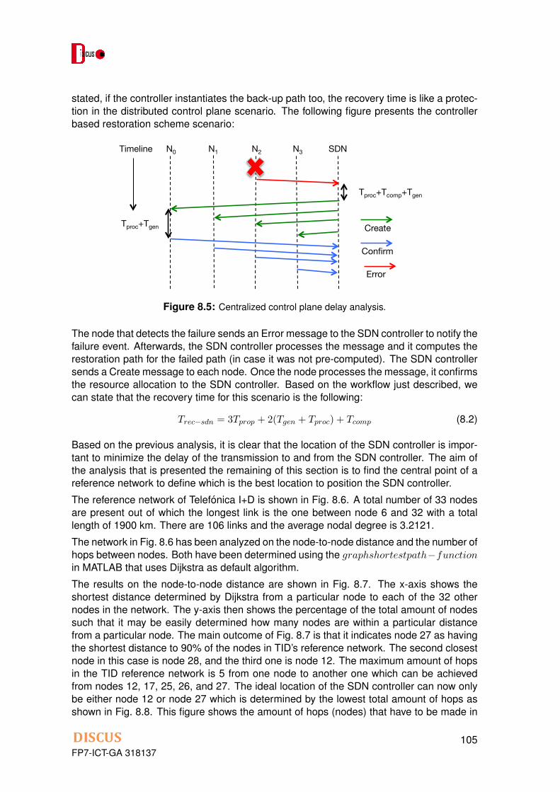
stated, if the controller instantiates the back-up path too, the recovery time is like a protec-tion in the distributed control plane scenario. The following figure presents the controllerbased restoration scheme scenario:

! !!

FP7!–!ICT!–!GA!318137! 15!DISCUS!!!

previously!stated,!if!the!controller!instantiates!the!back\up!path!too,!the!recovery!time!is!like!a!protection!in!the!distributed!control!plane!scenario.!!

The!following!figure!presents!the!controller!based!restoration!scheme!scenario:!

!Figure 1-6 Centralized control plane delay analysis

!

The!node!that!detects!the!failure!sends!an!Error!message!to!the!SDN!controller!to!notify!the!failure!event.!Afterwards,!the!SDN!controller!processes!the!message!and!it!computes!the!restoration!path!for!the!failed!path!(in!case!it!was!not!pre\computed).!The!SDN!controller!sends!a!Create!message!to!each!node.!Once!the!node!processes!the!message,!it!confirms!the!resource!allocation!to!the!SDN!controller.!Based!on!the!workflow!just!described,!we!can!state!that!the!recovery!time!for!this!scenario!is!the!following:!

Trec\sdn=3!Tprop!+!2!(Tgen+Tproc)!+Tcomp!

!

Based!on!the!previous!analysis,!it!is!clear!that!the!location!of!the!SDN!controller!is!important!to!minimize!the!delay!of!the!transmission!to!and!from!the!SDN!controller.!The!aim!of!the!analysis!that!is!presented!the!remaining!of!this!section!is!to!find!the!central!point!of!a!reference!network!to!define!which!is!the!best!location!to!position!the!SDN!controller.!!

The!reference!network!of!Telefónica!I+D!is!shown!in!Figure!7.!A!total!number!of!33!nodes!are!present!out!of!which!the!longest!link!is!the!one!between!node!6!and!32!with!a!total!length!of!1900!km.!There!are!106!links!and!the!average!nodal!degree!is!3.2121.!

N0 N1 N2 N3 Timeline SDN

Create

Confirm

Error

Tproc+Tcomp+Tgen

Tproc+Tgen

Figure 8.5: Centralized control plane delay analysis.

The node that detects the failure sends an Error message to the SDN controller to notify thefailure event. Afterwards, the SDN controller processes the message and it computes therestoration path for the failed path (in case it was not pre-computed). The SDN controllersends a Create message to each node. Once the node processes the message, it confirmsthe resource allocation to the SDN controller. Based on the workflow just described, wecan state that the recovery time for this scenario is the following:

Trec�sdn = 3Tprop + 2(Tgen + Tproc) + Tcomp (8.2)

Based on the previous analysis, it is clear that the location of the SDN controller is impor-tant to minimize the delay of the transmission to and from the SDN controller. The aim ofthe analysis that is presented the remaining of this section is to find the central point of areference network to define which is the best location to position the SDN controller.The reference network of Telefonica I+D is shown in Fig. 8.6. A total number of 33 nodesare present out of which the longest link is the one between node 6 and 32 with a totallength of 1900 km. There are 106 links and the average nodal degree is 3.2121.The network in Fig. 8.6 has been analyzed on the node-to-node distance and the number ofhops between nodes. Both have been determined using the graphshortestpath�functionin MATLAB that uses Dijkstra as default algorithm.The results on the node-to-node distance are shown in Fig. 8.7. The x-axis shows theshortest distance determined by Dijkstra from a particular node to each of the 32 othernodes in the network. The y-axis then shows the percentage of the total amount of nodessuch that it may be easily determined how many nodes are within a particular distancefrom a particular node. The main outcome of Fig. 8.7 is that it indicates node 27 as havingthe shortest distance to 90% of the nodes in TID’s reference network. The second closestnode in this case is node 28, and the third one is node 12. The maximum amount of hopsin the TID reference network is 5 from one node to another one which can be achievedfrom nodes 12, 17, 25, 26, and 27. The ideal location of the SDN controller can now onlybe either node 12 or node 27 which is determined by the lowest total amount of hops asshown in Fig. 8.8. This figure shows the amount of hops (nodes) that have to be made in

FP7-ICT-GA 318137105

Figure 8.6: The reference network of Telefonica I+D for SDN placement.

order to reach a particular node. It is clearly shown in Fig. 8.8 that node 12 (with a total of88 hops; node 27 has 96 hops) is the ideal location of the SDN controller in TID’s referencenetwork. ! !

!

FP7!–!ICT!–!GA!318137! 13!DISCUS!!!

!Figure 4: Distance between nodes vs. Percentage of nodes in TID’s reference network

!Figure 5: Total number of hops in TID’s reference network (shown per node)

!!! !

0 500 1000 1500 2000 2500 30000

0.1

0.2

0.3

0.4

0.5

0.6

0.7

0.8

0.9

1

Distance (km)

P(X<

x)

Node 1Node 2Node 3Node 4Node 5Node 6Node 7Node 8Node 9Node 10Node 11Node 12Node 13Node 14Node 15Node 16Node 17Node 18Node 19Node 20Node 21Node 22Node 23Node 24Node 25Node 26Node 27Node 28Node 29Node 30Node 31Node 32Node 33

Node 27

0 2 4 6 8 10 12 14 16 18 20 22 24 26 28 30 32 340

20

40

60

80

100

120

140

160

180

Node number

Tota

l num

ber o

f hop

s

Figure 8.7: Distance between nodes vs. Percentage of nodes in TID’s reference network.

8.5 Comparison between both approaches

Once both scenarios are analysed this section compares both control plane approachesbased on a given scenario.

8.5.1 GMPLS control plane delay values

The value of Tproc is set to 50 ms and the one of Tgen to 10 ms [95] . Moreover, thepropagation delay as well as the queuing delays are assumed to be negligible 3. Wehave compared the values in the reference with the results in Telefonica GMPLS control

FP7-ICT-GA 318137106

! !!

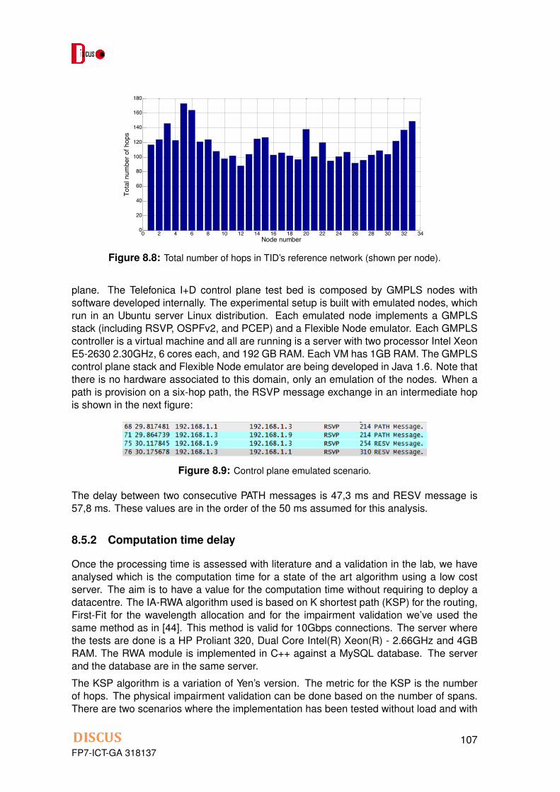
FP7!–!ICT!–!GA!318137! 13!DISCUS!!!

!Figure 4: Distance between nodes vs. Percentage of nodes in TID’s reference network

!Figure 5: Total number of hops in TID’s reference network (shown per node)

!!! !

0 500 1000 1500 2000 2500 30000

0.1

0.2

0.3

0.4

0.5

0.6

0.7

0.8

0.9

1

Distance (km)

P(X<

x)

Node 1Node 2Node 3Node 4Node 5Node 6Node 7Node 8Node 9Node 10Node 11Node 12Node 13Node 14Node 15Node 16Node 17Node 18Node 19Node 20Node 21Node 22Node 23Node 24Node 25Node 26Node 27Node 28Node 29Node 30Node 31Node 32Node 33

Node 27

0 2 4 6 8 10 12 14 16 18 20 22 24 26 28 30 32 340

20

40

60

80

100

120

140

160

180

Node number

Tota

l num

ber o

f hop

s

Figure 8.8: Total number of hops in TID’s reference network (shown per node).

plane. The Telefonica I+D control plane test bed is composed by GMPLS nodes withsoftware developed internally. The experimental setup is built with emulated nodes, whichrun in an Ubuntu server Linux distribution. Each emulated node implements a GMPLSstack (including RSVP, OSPFv2, and PCEP) and a Flexible Node emulator. Each GMPLScontroller is a virtual machine and all are running is a server with two processor Intel XeonE5-2630 2.30GHz, 6 cores each, and 192 GB RAM. Each VM has 1GB RAM. The GMPLScontrol plane stack and Flexible Node emulator are being developed in Java 1.6. Note thatthere is no hardware associated to this domain, only an emulation of the nodes. When apath is provision on a six-hop path, the RSVP message exchange in an intermediate hopis shown in the next figure:

Figure 8.9: Control plane emulated scenario.

The delay between two consecutive PATH messages is 47,3 ms and RESV message is57,8 ms. These values are in the order of the 50 ms assumed for this analysis.

8.5.2 Computation time delay

Once the processing time is assessed with literature and a validation in the lab, we haveanalysed which is the computation time for a state of the art algorithm using a low costserver. The aim is to have a value for the computation time without requiring to deploy adatacentre. The IA-RWA algorithm used is based on K shortest path (KSP) for the routing,First-Fit for the wavelength allocation and for the impairment validation we’ve used thesame method as in [44]. This method is valid for 10Gbps connections. The server wherethe tests are done is a HP Proliant 320, Dual Core Intel(R) Xeon(R) - 2.66GHz and 4GBRAM. The RWA module is implemented in C++ against a MySQL database. The serverand the database are in the same server.

The KSP algorithm is a variation of Yen’s version. The metric for the KSP is the numberof hops. The physical impairment validation can be done based on the number of spans.There are two scenarios where the implementation has been tested without load and with

FP7-ICT-GA 318137107

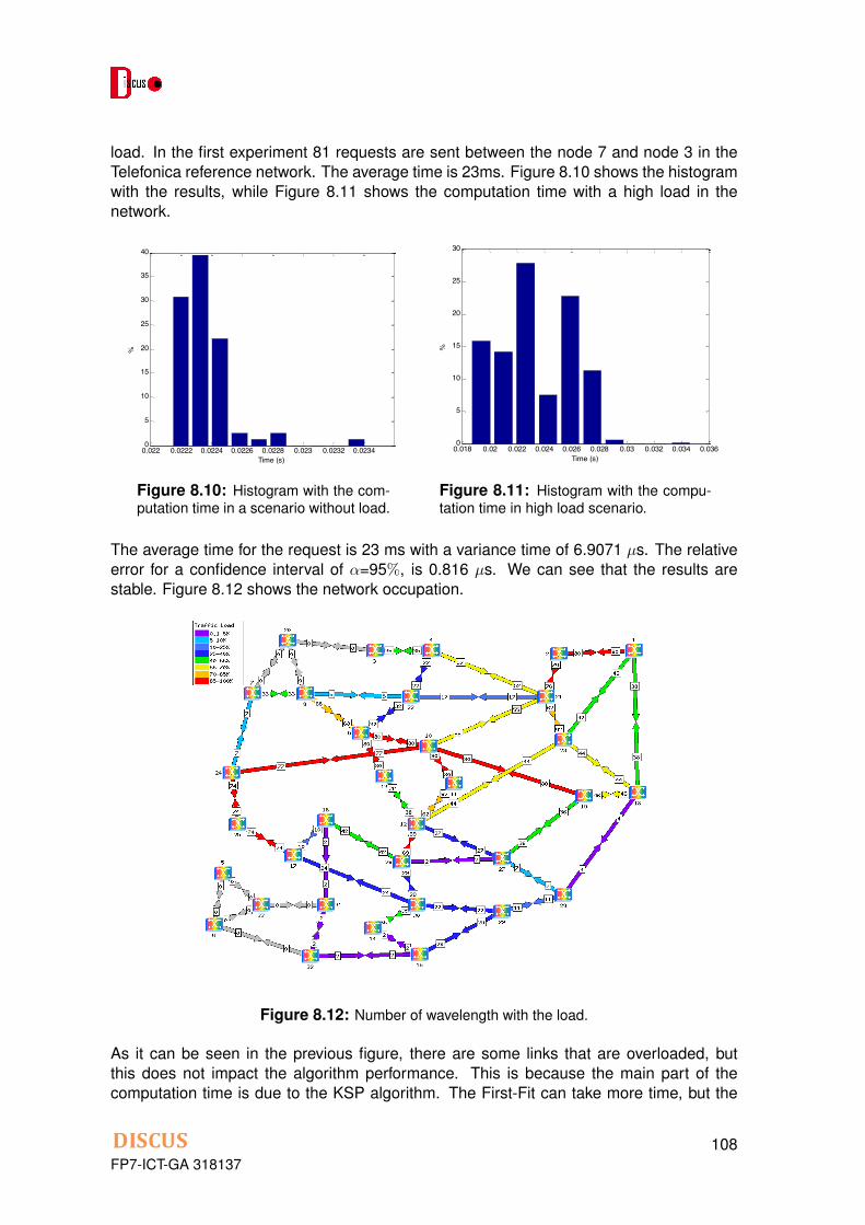
load. In the first experiment 81 requests are sent between the node 7 and node 3 in theTelefonica reference network. The average time is 23ms. Figure 8.10 shows the histogramwith the results, while Figure 8.11 shows the computation time with a high load in thenetwork.! !

!

FP7!–!ICT!–!GA!318137! 19!DISCUS!!!

!Figure 12: Histogram with the computation time in a scenario without load

Next!figure!shows!the!computation!time!with!a!high!load!in!the!network:!

!Figure 13: Histogram with the computation time in a scenario with high load

!The!average!time!for!the!request!is!23!ms!with!a!variance!time!of!6.9071!µs.!The!relative!error!for!a!confidence!interval!of!α=95%,!is!0.816!µs.!We!can!see!that!the!results!are!stable.!The!following!figure!shows!the!network!occupation:!!

0.022 0.0222 0.0224 0.0226 0.0228 0.023 0.0232 0.02340

5

10

15

20

25

30

35

40

%

Time (s)

0.018 0.02 0.022 0.024 0.026 0.028 0.03 0.032 0.034 0.0360

5

10

15

20

25

30

%

Time (s)

Figure 8.10: Histogram with the com-putation time in a scenario without load.

! !!

FP7!–!ICT!–!GA!318137! 19!DISCUS!!!

!Figure 12: Histogram with the computation time in a scenario without load

Next!figure!shows!the!computation!time!with!a!high!load!in!the!network:!

!Figure 13: Histogram with the computation time in a scenario with high load

!The!average!time!for!the!request!is!23!ms!with!a!variance!time!of!6.9071!µs.!The!relative!error!for!a!confidence!interval!of!α=95%,!is!0.816!µs.!We!can!see!that!the!results!are!stable.!The!following!figure!shows!the!network!occupation:!!

0.022 0.0222 0.0224 0.0226 0.0228 0.023 0.0232 0.02340

5

10

15

20

25

30

35

40

%

Time (s)

0.018 0.02 0.022 0.024 0.026 0.028 0.03 0.032 0.034 0.0360

5

10

15

20

25

30

%

Time (s)

Figure 8.11: Histogram with the compu-tation time in high load scenario.

The average time for the request is 23 ms with a variance time of 6.9071 µs. The relativeerror for a confidence interval of ↵=95%, is 0.816 µs. We can see that the results arestable. Figure 8.12 shows the network occupation.

Figure 8.12: Number of wavelength with the load.

As it can be seen in the previous figure, there are some links that are overloaded, butthis does not impact the algorithm performance. This is because the main part of thecomputation time is due to the KSP algorithm. The First-Fit can take more time, but the

FP7-ICT-GA 318137108

main contribution is KSP.

8.5.3 Assessment of central and distributed solution

Based on the values previously defined and justified, the recovery delay for the centralizedand the distributed recovery are compared. Figure 8.13 shows the recovery time for bothapproaches.! !

!

FP7!–!ICT!–!GA!318137! 21!

DISCUS!!!

!

Figure 15: Recovery time for SDN and GMPLS without propagation delay

GMPLS!is!as!fast!as!the!SDN!controller!only!when!the!number!of!hops!is!2.!The!reason!

is!that!the!SDN!controller!is!at!two!hops!from!any!failure.!The!reason!is!that!the!failure!is!

notified!to!the!controller,!which,!afterwards,!configures!the!nodes!with!the!failure.!

We!assumed!that!the!propagation!delay!in!the!control!plane!is!negligible.!However,!if!

this!value!were!250ms!and!the!average!number!of!hops!to!the!SDN!controller!where!5,!

the!delay!figure!would!be!different.!Next!figure!shows!the!recovery!time:!

!


!

The!SDN!approach!could!minimize!the!computation!time.!However!for!current!analysis!

the!impact!of!the!algorithm!is!so!small!that!it!won’t!benefit!this!scenario.!

Figure 8.13: Recovery time for SDNand GMPLS without propagation delay.

! !

!

FP7!–!ICT!–!GA!318137! 21!

DISCUS!!!

!


GMPLS!is!as!fast!as!the!SDN!controller!only!when!the!number!of!hops!is!2.!The!reason!

is!that!the!SDN!controller!is!at!two!hops!from!any!failure.!The!reason!is!that!the!failure!is!

notified!to!the!controller,!which,!afterwards,!configures!the!nodes!with!the!failure.!

We!assumed!that!the!propagation!delay!in!the!control!plane!is!negligible.!However,!if!

this!value!were!250ms!and!the!average!number!of!hops!to!the!SDN!controller!where!5,!

the!delay!figure!would!be!different.!Next!figure!shows!the!recovery!time:!

!


!

The!SDN!approach!could!minimize!the!computation!time.!However!for!current!analysis!

the!impact!of!the!algorithm!is!so!small!that!it!won’t!benefit!this!scenario.!

Figure 8.14: Recovery time for SDNand GMPLS with propagation delay.

GMPLS is as fast as the SDN controller only when the number of hops is 2. The reasonis that the SDN controller is at two hops from any failure. The reason is that the failureis notified to the controller, which, afterwards, configures the nodes with the failure. Weassumed that the propagation delay in the control plane is negligible. However, if thisvalue were 250ms and the average number of hops to the SDN controller where 5, thedelay figure would be different. Figure 8.14 shows the recovery time.

The SDN approach could minimize the computation time. However for current analysis theimpact of the algorithm is so small that it won’t benefit this scenario.

8.6 Conclusions

Control plane architecture defined in DISCUS project considered distributed control planefor the core part. The distributed control plane is more resilient that the centralized ap-proach, but if the SDN controller is in two datacentres with multiple VMs, the resilienceproblems are minimized. Based on the analysis done in this document with realistic sce-narios, the controller-based approach is very promising as it minimized the recovery time.This validates the DISCUS control plane architecture not only in terms of functional fea-tures, but also in resilience scenarios.

FP7-ICT-GA 318137109

Chapter 9

Conclusions

This deliverable presented a number of optimization models and methods that can be usedto dimension the core network segment of the DISCUS architecture. The focus of thesemodels has been mainly on cost minimisation and on the maximisation of the resiliencylevels that can be offered to the provisioned services. The scenarios considered includedboth network design and in-operation optimization problems.

The contribution of the deliverable is manyfold. This was done on purpose since the mainobjective of the set of studies carried out so far in the project was to assess the perfor-mance of a wide set of options in terms of core network optimization strategies. The planis to identify the most promising ones to be used in the optimization work for the final con-solidated/integrated optical core design phase, that will be presented in Deliverable D7.7.A few concluding remarks about the various contributions presented in this deliverable arepresented next.

Chapter 2 provided a consolidated model of cost and hardware including core photonicswitching, signal regeneration, and Raman amplification, while Chapter 3 presented meth-ods that can be used to solve multi-layer core network design problems in order to assessthe impact of the DISCUS optical island concept. It was found that optical islands out-perform architectures based on aggregating (grooming) traffic towards an inner core oncethe traffic volume exceeds a certain threshold. These results are dependent on the costmodel, the number of metro-core nodes, and the available channel capacities (40G, 100G,400G).

Chapter 4 presented planning approaches for providing core-network survivability in thepresence of single link- and nodefailures, individual node component faults and deliberatephysical-layer attacks targeting service disruption. On the other hand Chapter 5 lookedmore into the problem of providing resiliency to services in the presence of dynamic trafficwhere both single and double link failures scenarios where considered.

Chapter 6 presented a study on the dimensioning of metro/core networks with dual-homedaccess under the assumption of single metro/core node failure scenario. The resultsdemonstrate that multilayer restoration combined with the right amount of transponderoverprovisioning allows to achieve average connection availability levels very similar to theones achieved by dedicated path protection but with lower service blocking levels and atthe same time using a lower number of WDM transponders.

Chapter 7 evaluated the impact that energy-efficient techniques have on the componentlifetime in an optical backbone network. The focus was on understanding the effects ofputting EDFAs into sleep mode. The study showed that frequent on/sleep transitions mayhave a negative impact on the EDFA failure rate. Finally, Chapter 8 presented a studyevaluating centralized versus distributed control plane architectures in terms of recoverytime offered to services. It was found that the propagation delay of control messageshas a non trascurable impact on the overall recovery time. For this reason the controllerplacement within the network needs to be carefully considered.

FP7-ICT-GA 318137110

Appendix A

Acronyms

Acronym Explanation

AA-DPP Attack-Aware Dedicated Path ProtectionAA-DPP-H Attack-Aware Dedicated Path Protection HeuristicAF Accelleration FactorAG Attack GroupAkNLPP All-Pairs k Node-Disjoint Length-Bounded Paths ProblemAoD Architecture on DemandAWG Arrayed Waveguide GratingBPSK Binary Phase-Shift KeyingBV-WSS Bandwidth-Variable Wavelength Selective SwitchesBR Backup ReprovisioningBSPP Backup Server via Physically disjoint PathCO Central OfficeCTE Coefficient of Temperature ExpansionDC Data CenterDGE Digital Gain EqualizerDH-DPP Dual Homin Dedicated Path ProtectionDH-PR-AVG Dual Homing Path Restoration AverageDH-PR-MAX Dual Homing Path Restoration MaxDH-PR-UNP Dual Homing Path Restoration UnprotectedDP-QPSK Dual Polarization Quadrature Phase-Shift KeyingDPP Dedicated Path ProtectionDPP-EFS Dedicated Path Protection with Enforced Fiber SwitchingDPP-SP Dedicated Path Protection with Shortest Path routingDWDM Dense WDMEDFA Erbium Doped Fiber AmplifiersEFS Enforced Fiber SwitchingFCC Federal Communication CommissionFIT Failure In TimeFS Fiber SwitchingGB GigabyteGbps Gigabit per secondHW HardwareH-W Hard-WiredKSP K shortest pathIA-RWA Impairment Aware Routing and Wavelength AssignmentICU Idealist Cost UnitIP Internet ProtocolILP Integer Linear ProgramIX Internet Exchange, Peering Point

FP7-ICT-GA 318137111

LE Local ExchangeLP Linear ProgramLR-PON Long Reach PONLSP Labeled Switched PathMC Metro-coreMbps Megabit per secondMDD Minimum Distance DesignMDT Mean Down TimeMEMS Micro Electro Mechanical SwitchesMIP Mixed Integer Program (MILP)MILP Mixed ILPGMPLS Generalized Multi-Protocol Label SwitchingMPLS Multi-Protocol Label SwitchingMPLS-TP MPLS Transport ProfileODN Optical Distribution NetworkOEO Optical-to-Electrical-to-OpticalOLT Optical Line TerminationOLA Optical Line AmplifierONU Optical Network UnitOOK On-Off KeyingOSPF Open Shortest Path FirstOXC Optical Cross ConnectPCE Path Computation ElementPCEP Path Computation Element communication ProtocolPON Passive Optical NetworkPR Path RestorationQPSK Quadrature Phase-Shift KeyingROADM Reconfigurable Optical Add Drop MultiplexerRSVP Resource Reservation ProtocolRWA Routing and Wavelength AssignmentSDN Software Defined NetworksSD Standard DefinitionSSS Spectrum Selective SwitchSSON Spectrum Switched Optical NetworksTbps Terabit per secondTE Traffic EngineeringUK United KingdomVOA Variale Optical AttenuatorVTD Virtual Topology DesignWDM Wavelength Division MultiplexingWP2/WP4/WP7 DISCUS Work Package 2/4/7WPA-LR Weighted Power Aware Lightpath RoutingWSON Wavelength Switched Optical NetworksWSS Wavelength Selective Switch

FP7-ICT-GA 318137112

Appendix B

Versions

Version1 Date submitted CommentsV1.0 30/04/2015 First version sent to the commission

1Last row represents the current document version

FP7-ICT-GA 318137113

Bibliography

[1] Gurobi Optimizer. URL http://www.gurobi.com/.

[2] Net2Plan – The open-source network planner. URL http://www.net2plan.com.

[3] IDEALIST, Deliverable 1.1, Elastic Optical Network Architecture: reference scenario,cost and planning. Technical report, IST IP IDEALIST: Industry-Driven Elastic andAdaptive Lambda Infrastructure for Service and Transport Network, 2013.

[4] DISCUS, Deliverable 7.2, Optical Island Description. Technical report, The DISCUSProject (FP7 Grant 318137), 2013.

[5] DISCUS, Deliverable 2.4, Progress report on traffic and service modelling. Technicalreport, The DISCUS Project (FP7 Grant 318137), 2014.

[6] DISCUS, Deliverable 2.6, Architectural optimization for different geo-types . Technicalreport, The DISCUS Project (FP7 Grant 318137), 2014.

[7] DISCUS, Deliverable 6.1, First Report on the Specification of the Metro/Core NodeArchitecture. Technical report, The DISCUS Project (FP7 Grant 318137), 2014.

[8] DISCUS, Deliverable 6.2, Report on the design and control mechanism of a 3-stageoptical switch. Technical report, The DISCUS Project (FP7 Grant 318137), 2014.

[9] DISCUS, Deliverable 7.1, Power Consumption Studies. Technical report, The DISCUSProject (FP7 Grant 318137), 2014.

[10] DISCUS, Deliverable 7.2, Preliminary quantitative results for flat optical network. Tech-nical report, The DISCUS Project (FP7 Grant 318137), 2014.

[11] DISCUS, Deliverable 2.8, DISCUS end-to-end techno-economic model. Technical re-port, The DISCUS Project (FP7 Grant 318137), 2015, in preparation.

[12] DISCUS, Deliverable 6.5, Final report on the specification of the metro/core nodearchitecture. Technical report, The DISCUS Project (FP7 Grant 318137), 2015, inpreparation.

[13] A. Farrel, et al. A Path Computation Element (PCE) Based Architecture, 2006. URLhttps://tools.ietf.org/html/rfc4655.

[14] Sandu Abeywickrama, Marija Furdek, Paolo Monti, Avishek Nag, and Elaine Wong.Dual-homing based protection for enhanced network availability and resource effi-ciency. In Asia Communications and Photonics Conference 2014, page ATh1H.6.Optical Society of America, 2014.

[15] J. Ahmed and S. Nawaz. Proc. ncet. In POSE: A New Discrete Event Optical Simu-lator for the Java Platform, 2004.

[16] J. Ahmed, C. Cavdar, P. Monti, and L. Wosinska. A dynamic bulk provisioning frame-work for concurrent optimization in pce-based wdm networks. Lightwave Technology,Journal of, 30(14):2229–2239, July 2012.

FP7-ICT-GA 318137114

http://www.gurobi.com/

http://www.net2plan.com

https://tools.ietf.org/html/rfc4655

[17] J. Ahmed, C. Cavdar, P. Monti, and L. Wosinska. Hybrid survivability schemes achiev-ing high connection availability with a reduced amount of backup resources [invited].Optical Communications and Networking, IEEE/OSA Journal of, 5(10):A152–A161,Oct 2013.

[18] Jawwad Ahmed, Paolo Monti, and Lena Wosinska. Benefits of connection requestbundling in a pce-based wdm network. In Proc. of European Conference on Networksand Optical Communications (NOC), 2009.

[19] Jawwad Ahmed, Paolo Monti, Lena Wosinska, and Salvatore Spadaro. Enhancingrestoration performance using service relocation in pce-based resilient optical clouds.In Optical Fiber Communication Conference, page Th3B.3. Optical Society of Amer-ica, 2014.

[20] Norberto Amaya, Georgios Zervas, and Dimitra Simeonidou. Architecture on demandfor transparent optical networks. In ICTON, pages 1–4, 2011.

[21] Norberto Amaya, Georgios Zervas, and Dimitra Simeonidou. Introducing Node Archi-tecture Flexibility for Elastic Optical Networks. IEEE/OSA Journal of Optical Commu-nications and Networking, 5(6):593–608, 2013.

[22] R. Andersen, Fan Chung, A. Sen, and Guoliang Xue. On disjoint path pairs withwavelength continuity constraint in wdm networks. In INFOCOM 2004. Twenty-thirdAnnualJoint Conference of the IEEE Computer and Communications Societies, vol-ume 1, pages –535, March 2004.

[23] Takashi Anzawa, Qiang Yu, Masanori Yamagiwa, Tadahiro Shibutani, and MasakiShiratori. Power cycle fatigue reliability evaluation for power device using coupledelectrical-thermal-mechanical analysis. In Proc. of the ITHERM, Orlando, USA, May2008.

[24] S. Arrhenius. Uber die Reaktionsgeschwindigkeit bei der Inversion von Rohrzuckerdurch Sauren. Wilhelm Engelmann, 1889.

[25] F. Bayle and A Mettas. Temperature acceleration models in reliability predictions:Justification & improvements. In Proc. of the RAMS, San Jose, USA, January 2010.

[26] Pietro Belotti, Antonio Capone, Giuliana Carello, and Frederico Malucelli. Multi-layerMPLS network design: The impact of statistical multiplexing. Computer Networks, 52(6):1291–1307, 2008.

[27] Richard Blish and Noel Durrant. Semiconductor device reliability failure models. In-ternational Sematech Technology Transfer #00053955A-XFR, May 2000.

[28] R. Bolla, R. Bruschi, F. Davoli, and F. Cucchietti. Energy efficiency in the futureinternet: a survey of existing approaches and trends in energy-aware fixed networkinfrastructures. IEEE Communications Surveys & Tutorials, 13(2):223–244, 2011.

[29] L. Chiaraviglio and M. Listanti. On the interplay between sleep modes and devicelifetime in telecommunication networks. In Proc. of the EINS Workshop on Under-standing the Interplay Between Sustainability, Resilience, and Robustness in Net-works (USRR), Ghent, Belgium, April 2014.

FP7-ICT-GA 318137115

[30] Luca Chiaraviglio, Antonio Cianfrani, Angelo Coiro, Marco Listanti, Josip Lorincz, andMarco Polverini. Increasing device lifetime in backbone networks with sleep modes.In Proc. of the SoftCOM, Primosten, Croatia, September 2013.

[31] Biing-Feng Wang Chih-Chiang Yu, Chien-Hsin Lin. Improved algorithms for findinglength-bounded two vertex-disjoint paths in a planar graph and minmax k vertex-disjoint paths in a directed acyclic graph. Journal of Computer and System Sciences,76:697–708, 2010.

[32] X. Chu, B. Li, and Z. Zhang. A dynamic rwa algorithm in a wavelength-routed all-optical network with wavelength converters. In INFOCOM 2003. Twenty-Second An-nual Joint Conference of the IEEE Computer and Communications. IEEE Societies,volume 3, pages 1795–1804 vol.3, March 2003.

[33] Cisco. Cisco Visual Networking Index: Forecast and Methodology, 2013– 2018, 2015. URL http://http://www.cisco.com/c/en/us/solutions/

collateral/service-provider/ip-ngn-ip-next-generation-network/white_

paper_c11-481360.html.

[34] (L. F.) Coffin Jr. and U.S. Atomic Energy Commission and General Electric Company.A Study of the Effects of Cyclic Thermal Stresses on a Ductile Metal. Knolls AtomicPower Laboratory, 1953.

[35] Ayse K Coskun, Richard Strong, Dean M Tullsen, and Tajana Simunic Rosing. Eval-uating the impact of job scheduling and power management on processor lifetime forchip multiprocessors. In Proc. of the SIGMETRICS/Performance, Seattle, USA, June2009.

[36] C. Develder, M. De Leenheer, B. Dhoedt, M. Pickavet, D. Colle, F. De Turck, and P. De-meester. Optical networks for grid and cloud computing applications. Proceedings ofthe IEEE, 100(5):1149–1167, May 2012.

[37] C. Develder, J. Buysse, B. Dhoedt, and B. Jaumard. Joint dimensioning of serverand network infrastructure for resilient optical grids/clouds. Networking, IEEE/ACMTransactions on, 22(5):1591–1606, Oct 2014.

[38] M. Nishan Dharmaweera, Rajendran Parthiban, and Y. Ahmet Sekercioglu. Towardsa power-efficient backbone network: The state of research. IEEE CommunicationsSurveys & Tutorials, 2014. accepted for publication.

[39] E.W. Dijkstra. A Note on Two Problems in Connection with Graphs. NumerischeMathematik, 1(1):269–271, 1959.

[40] Matija Dzanko, Marija Furdek, Norberto Amaya, Georgios Zervas, Branko Mikac, andDimitra Simeonidou. Self-healing Optical Networks with Architecture on DemandNodes. In European Conference and Exibition on Optical Communication, pages1–3, 2013.

[41] Matija Dzanko, Marija Furdek, Georgios Zervas, and Dimitra Simeonidou. Evalu-ating Availability of Optical Networks Based on Self-Healing Network Function Pro-grammable ROADMs. IEEE/OSA Journal of Optical Communications and Network-ing, 6(11):974–987, 2014.

FP7-ICT-GA 318137116

[42] M. Dzanko, M. Furdek, N.A. Gonzalez, G. Zervas, B. Mikac, and D. Simeonidou.Experimental demonstration and benefits of self-healing hard-wired and syntheticroadms. In Optical Fiber Communications Conference and Exhibition (OFC), 2014,pages 1–3, March 2014.

[43] W. Engelmeier. Solder Joints in Electronics: Design for Reliability. URL http://

analysistech.com/downloads/SolderJointDesignForReliability.pdf.

[44] D. Alvarez et al. Utilization of temporary reservation of path computed resources formulti-domain pce protocols in wdm networks. In Network of the Future Conference,Nov 2011.

[45] M. Garrich et al. Architecture on demand: synthesis and scalability. In Proc. of IEEEOptical Network Design and Modeling, ONDM, 2012.

[46] N. Amaya et al. Architecture on demand for transparent optical networks. In Proc. ofIEEE International Conference on Transparent Optical Networks, ICTON, 2011.

[47] Y. Wang et al. Multi-granular optical switching: A classified overview for the past andfuture. IEEE Communications Surveys and Tutorials, 14(3):698–713, 2013.

[48] Mabel P. Fok, Z. Wang, Y. Deng, and Paul R. Prucnal. Optical layer security in fiber-optic networks. IEEE T. Inf. Foren. Sec, 6(3):725–736, 2011.

[49] Marija Furdek, Nina Skorin-Kapov, Szilard Zsigmond, and Lena Wosinska. Vulnera-bilities and security issues in optical networks. In ICTON, pages 1–4, 2014.

[50] Miquel Garrich, Norberto Amaya, Georgios Zervas, Paolo Giaccone, and DimitraSimeonidou. Architecture on Demand: Synthesis and Scalability. In InternationalConference on Optical Network Design and Modeling, pages 1–6, 2012.

[51] Miquel Garrich, Norberto Amaya, Georgios Zervas, Paolo Giaccone, and DimitraSimeonidou. Power Consumption Analysis of Architecture on Demand. In EuropeanConference and Exhibition on Optical Communication, pages 1–3, 2012.

[52] Filip Idzikowski, Luca Chiaraviglio, Raul Duque, Felipe Jimenez, and EstherLe Rouzic. Green horizon: Looking at backbone networks in 2020 from the per-spective of network operators. In Proc. of the ICC, Budapest, Hungary, June 2013.

[53] ITU-T meeting Bundang, South Korea. Controller based protection, 2015.

[54] J.-L. Izquierdo Zaragoza and P. Pavon-Marino. Assessing ip vs optical restorationusing the open-source net2plan tool. In Telecommunications Network Strategy andPlanning Symposium (Networks), 2014 16th International, pages 1–6, Sept 2014.

[55] JEDEC Solid State Technology Association et al. Failure mechanisms and models forsemiconductor devices. JEDEC Publication JEP122-C, March 2006.

[56] P. N. Ji and Y. Aono. Colorless and directionless multi-degree reconfigurable opticaladd/drop multiplexers. In Wireless and Optical Communications Conference, pages1–5, 2010.

[57] R.E Tarjan J.W. Suurballe. A quick method for finding shortest pairs of disjoint paths.Networks, 14(2):325–336, 1984.

FP7-ICT-GA 318137117

http://analysistech.com/downloads/SolderJointDesignForReliability.pdf

http://analysistech.com/downloads/SolderJointDesignForReliability.pdf

[58] Ken-Ichi Kitayama, M. Sasaki, S. Araki, M. Tsubokawa, A. Tomita, K. Inoue, K. Ha-rasawa, Y. Nagasako, and A. Takada. Security in photonic networks: threats andsecurity enhancement. IEEE/OSA Journal of Lightwave Technology, 29(21):3210–3222, 2011.

[59] Arie M. C. A. Koster, Sebastian Orlowski, Christian Raack, Georg Baier, and ThomasEngel. Single-layer Cuts for Multi-Layer Network Design Problems. In Bruce Golden,Subramanian Raghavan, and Edward Wasil, editors, Telecommunications ModelingPolicy and Technology, also ZIB Report ZR-07-21, chapter 1, pages 1–23. Springer,College Park, MD, U.S.A., 2008. Selected proceedings of the 9th INFORMS Telecom-munications Conference.

[60] Arie M. C. A. Koster, Sebastian Orlowski, Christian Raack, Georg Baier, ThomasEngel, and Pietro Belotti. Branch-and-cut techniques for solving realistic two-layernetwork design problems. In Arie M. C. A. Koster and Xavier Munoz, editors, Graphsand Algorithms in Communication Networks, chapter 3, pages 95–118. Springer, De-cember 2009.

[61] G. Landi, N. Ciulli, J. Buysse, K. Georgakilas, M. Anastasopoulos, A. Tzanakaki,C. Develder, E. Escalona, D. Parniewicz, A. Binczewski, and B. Belter. A networkcontrol plane architecture for on-demand co-provisioning of optical network and itservices. In Future Network Mobile Summit (FutureNetw), July 2012.

[62] U. Mandal, M. Habib, Shuqiang Zhang, B. Mukherjee, and M. Tornatore. Greening thecloud using renewable-energy-aware service migration. Network, IEEE, 27(6):36–43,November 2013.

[63] S. S. Manson. Behavior of materials under conditions of thermal stress. NACA Report1170, 1954.

[64] Sara Mattia. Solving survivable two-layer network design problems by metric inequal-ities. Computational Optimization and Applications, pages 1–26, 2010.

[65] Sara Mattia. A Polyhedral Study of the Capacity Formulation of the Multilayer NetworkDesign Problem. Networks, 62(1):17–26, 2013.

[66] Ullrich Menne, Christian Raack, and Roland Wessaly. Impact of technology, architec-ture, and price trends on optimal multi-layer network designs. In Proceedings of 16thInternational Conference on Optical Networking Design and Modeling (ONDM 2012),ONDM 2012, 2012, submitted. submitted.

[67] A. Muhammad, G. S. Zervas, N. Amaya, D. E. Simeonidou, and R. Forchheimer. Cost-efficient design of flexible optical networks implemented by architecture on demand.In Proc. of IEEE/OSA Optical Fiber Communication Conference and Exposition, OFC,2014.

[68] Ajmal Muhammad, Georgios Zervas, Norberto Amaya, Dimitra Simeonidou, andRobert Forchheimer. Introducing Flexible and Synthetic Optical Networking: Plan-ning and Operation Based on Network Function Programmable ROADMs. IEEE/OSAJournal of Optical Communications and Networking, 6(7):635–648, 2014.

[69] Avishek Nag, David B. Payne, and Marco Ruffini. N:1 protection design for minimis-ing olts in resilient dual-homed long-reach passive optical network. In Optical FiberCommunication Conference, page Tu2F.7. Optical Society of America, 2014.

FP7-ICT-GA 318137118

[70] K.C. Norris and A.H. Lanzberg. Reliability of controlled collapse interconnections.IBM Journal of Research and Development, 13(3):266–271, May 1969.

[71] E. Oki. Linear Programming and Algorithms for Communication Networks A PracticalGuide to Network Design, Control, and Management. CRC Press, 2013.

[72] Sebastian Orlowski. Optimal Design of Survivable Multi-layer Telecommunication Net-works. PhD thesis, Technische Universitat Berlin, May 2009.

[73] Sebastian Orlowski, Arie M. C. A. Koster, Christian Raack, and Roland Wessaly. Two-layer Network Design by Branch-and-Cut featuring MIP-based Heuristics. In Proceed-ings of the 3rd International Network Optimization Conference (INOC 2007), Spa,Belgium, 2007.

[74] Pablo Pavon-Marino and Jose-Luis Izquierdo-Zaragoza. On the role of open-sourceoptical network planning. In Optical Fiber Communication Conference, page Th1E.1.Optical Society of America, 2014.

[75] Y. Peng, Z. Sun, S. Du, and K. Long. Propagation of all-optical crosstalk attack intransparent optical networks. Optical Engineering, 50(8):085002.1–3, 2011.

[76] Andrew Eugene Perkins. Investigation and prediction of solder joint reliability for ce-ramic area array packages under thermal cycling, power cycling, and vibration envi-ronments. PhD thesis, Georgia Institute of Technology, May 2007.

[77] Michal Pioro and Deepankar Medhi. Routing, Flow, and Capacity Design in Commu-nication and Computer Networks. Morgan Kaufmann Publishers, 2004.

[78] Diane E. Hodges Popp, Andrew Mawer, and Gabriel Presas. Flip chip PBGA sol-der joint reliability: power cycling versus thermal cycling. Motorola SemiconductorProducts Sector, Austin, TX, 2005.

[79] J. S. Arora R. T. Marler. The weighted sum method for multi-objective optimization:new insights. Structural and Multidisciplinary Optimization, 41(6):853–862, 2010.

[80] S. Ramamurthy and B. Mukherjee. Survivable wdm mesh networks. part i-protection.In INFOCOM ’99. Eighteenth Annual Joint Conference of the IEEE Computer andCommunications Societies. Proceedings. IEEE, volume 2, pages 744–751 vol.2, Mar1999.

[81] S. Ramamurthy, L. Sahasrabuddhe, and B. Mukherjee. Survivable wdm mesh net-works. J. Lightwave Technol., 21(4):870, Apr 2003.

[82] Franz Rambach, Beate Konrad, Lars Dembeck, Ulrich Gebhard, Matthias Gunkel,Marco Quagliotti, Laura Serra, and Vıctor Lopez. A Multilayer Cost Model for Metro/-Core Networks. J. OPT. COMMUN. NETW., 5(3):210–225, 2013.

[83] Ridha Rejeb, Mark S. Leeson, and Roger Green. Fault and attack management inall-optical networks. IEEE Communications Magazine, 44(11):79–86, 2006.

[84] Ridha Rejeb, Mark S. Leeson, Carmen Mas Machuca, and Ioannis Tomkos. Controland management issues in all-optical networks. Journal of Networks, 5(2):132–139,2010.

FP7-ICT-GA 318137119

[85] D.A. Schupke and Franz Rambach. A link-flow model for dedicated path protectionwith approximative availability constraints. Communications Letters, IEEE, 10(9):679–681, Sept 2006.

[86] Qingya She, Xiaodong Huang, Qiong Zhang, Yi Zhu, and J.P. Jue. Survivable traf-fic grooming for anycasting in wdm mesh networks. In Global TelecommunicationsConference, 2007. GLOBECOM ’07. IEEE, pages 2253–2257, Nov 2007.

[87] Deepinder Sidhu, Raj Nair, and Shukri Abdallah. Finding disjoint paths in networks.SIGCOMM Comput. Commun. Rev., 21(4):43–51, August 1991. ISSN 0146-4833.

[88] Jane M. Simmons. Optical Network Design and Planning. Springer Publishing Com-pany, Incorporated, 1 edition, 2008. ISBN 0387764755, 9780387764757.

[89] L. Song, J. Zhang, and B. Mukherjee. A comprehensive study on backup-bandwidthreprovisioning after network-state updates in survivable telecom mesh networks. Net-working, IEEE/ACM Transactions on, 16(6):1366–1377, Dec 2008.

[90] J.W. Suurballe. Disjoint paths in a network. NETWORKS, 4(2):125–145, 1974.

[91] Ward Van Heddeghem, Filip Idzikowski, Willem Vereecken, Didier Colle, Mario Pick-avet, and Piet Demeester. Power consumption modeling in optical multilayer net-works. Photonic Network Communications, 24(2):86–102, October 2012.

[92] Jean-Philippe Vasseur, Mario Pickavet, and Piet Demeester. Network Recovery: Pro-tection and Restoration of Optical, SONET-SDH, IP, and MPLS. Morgan KaufmannPublishers Inc., San Francisco, CA, USA, 2004. ISBN 012715051X.

[93] P. Wiatr, P. Monti, and L. Wosinska. Power savings versus network performance indynamically provisioned WDM networks. IEEE Communications Magazine, 50(5):48–55, May 2012. ISSN 0163-6804. doi: 10.1109/MCOM.2012.6194382.

[94] Pawel Wiatr, Jiajia Chen, Paolo Monti, and Lena Wosinska. Energy efficiency andreliability tradeoff in optical core networks. In Proc. of the OFC, San Francisco, USA,March 2014.

[95] Jing Wu and Michel Savoie. Recovery from control plane failures in the rsvp-te sig-naling protocol. Computer Communications, 34(16):1956–1967, October 2011.

[96] Yoshiyuki Yamada, Hiroshi Hasegawa, and Ken-Ichi Sato. Survivable HierarchicalOptical Path Network Design With Dedicated Wavelength Path Protection. IEEE/OSAJournal of Lightwave Technology, 29(21):3196–3209, 2011.

[97] Shengli Yuan and J.P. Jue. Dynamic lightpath protection in wdm mesh networks underwavelength continuity constraint. In Global Telecommunications Conference, 2004.GLOBECOM ’04. IEEE, volume 3, pages 2019–2023 Vol.3, Nov 2004.

[98] J. Zhang, K. Zhu, and B. Mukherjee. Backup reprovisioning to remedy the effectof multiple link failures in wdm mesh networks. Selected Areas in Communications,IEEE Journal on, 24(8):57–67, Aug 2006.

[99] Mark Ziegelmann. Constrained Shortest Paths and Related Problems - ConstrainedNetwork Optimization. VDM Verlag, Saarbrucken, Germany, Germany, 2007. ISBN3836446332, 9783836446334.

FP7-ICT-GA 318137120

core network optimization and resiliency strategies

Documents