portfolio - mark alan weir of copper in brass by atomic absorption spectroscopy ... spectroscopic...
TRANSCRIPT

Portfolio
Mark A. Weir 546 Scenic Dr. Ashland, OR 97520 619.980.8220 [email protected]
Dual Degrees from Southern Oregon University:
Biochemistry (ACS Certified)
Biology, Cell/Molecular option (Honors)
Table of Contents
Core Academics .................................................................................................................. 4
Core Requirements .......................................................................................................... 4
General Education Requirements .................................................................................... 4
Electives .......................................................................................................................... 5
Oral Presentations ............................................................................................................... 6
Instrument Proficiency ......................................................................................................... 7
Gas Chromatography – Mass Spectroscopy .................................................................... 7
Nuclear Magnetic Resonance Spectroscopy .................................................................... 7
Ultraviolet-Visible Spectroscopy ....................................................................................... 7
High-Performance Liquid Chromatography ...................................................................... 7
Atomic Absorption Spectroscopy ..................................................................................... 7
Inductively Coupled Plasma – Optical Emission Spectrometry ......................................... 7
Fourier Transform – Infrared Spectroscopy ...................................................................... 8
Gas Exchange & Fluorescence ........................................................................................ 8
DNA Sequencer ............................................................................................................... 8
Determination of Ethanol in Wine by Gas Chromatography .......................................... 9
Fractional Distillation .................................................................................................. 15
A Comparison of Fatty Acids Isolated from the Triglycerides of Grain-Fed and Grass-Fed Beef .......................................................................................................................... 18
Sequence Determination of an Unknown Dipeptide .................................................... 30
Simultaneous Determination of Caffeine and Benzoic Acid in Mountain Dew by Ultraviolet Spectroscopy ................................................................................................... 41
Stability of Aspirin by Reversed-Phase HPLC ............................................................. 49
Determination of Copper in Brass by Atomic Absorption Spectroscopy ...................... 63
Constituents of Lithia Water ........................................................................................ 70
Symmetry, Point Groups, and Infrared Spectroscopy ................................................. 77
Effects of Varied Nitrogen Treatments on Growth and Physiology among Raphanus sativus .............................................................................................................................. 82
Isolation and Identification of Putative Plant Growth Promoting Bacterial Isolates Containing the acdS (ACC Deaminase) Gene .................................................................. 93
Computer Skills ............................................................................................................... 105
Molecular Modeling ...................................................................................................... 105
Spectroscopic Analysis ................................................................................................ 105

Programing and Mathematics ...................................................................................... 105
Spreadsheets and Word Processing ............................................................................ 105
Genetics....................................................................................................................... 105
Research ......................................................................................................................... 106
Cooperative Learning ...................................................................................................... 108
Honors and Awards ......................................................................................................... 109
Additional References .......................................................... Error! Bookmark not defined.
Core Academics
Below is the core, general and elective courses taken to satisfy an ACS Biochemistry degree and a Cellular /Molecular Biology at Southern Oregon University.
Core Requirements
General Biology / General Biology Lab (BI 211, 212, 213)
General Chemistry / General Chemistry Lab (CH 221, 222, 223, 224, 225, 226)
Calculus I, II, III (CH 251, 252, 253), Differential Equations (MT 321)
General Physics / General Physics Lab (PH 221, 222, 223, 224, 225, 226)
Chemical Research Communication (CH 314, 315, 316)
Organic Chemistry / Organic Chemistry Labs (CH 334, 335, 336, 337, 340, 341)
Computer Applications in Chemistry (CH 371)
Physical Chemistry (CH 441, 442, 443)
Physical-Chemical Measurements (CH 444)
Analytical Chemistry / Analytical Chemistry Lab (CH 421, 422)
Instrumental Analysis / Instrumental Analysis Lab (CH 425, 426)
Inorganic Chemistry / Inorganic Chemistry Lab (CH 411, 414)
Molecular Biology (BI 425), Genetics (BI 341)
Senior Capstone (CH 497, 498, 499)
General Education Requirements
Cultural Anthropology (Anth 213)
World Civilizations (HST 110)
English Composition (WR 121, 122)
Economics (EC 201, 202)
Law, Politics and Constitution (PS 202)
Sociological Imagination (SOC 204)
Public Speaking (COMM 210)
International Business – (BA 477)
Science and the Young Child – (ED 437)
Corporate Sustainability – (BA 490)
Electives
Human Anatomy & Physiology I,II, III (BI 231, 232, 233)
Spanish 1st and 2nd year (SPAN 101, 102, 103, 201, 202)
Microbiology (BI 234)
Cell Biology (BI 342)
Developmental Biology (BI 343)
Plant Ecology (BI 454)
Plant Physiology (BI 331)
Evolution (446)
Intro Ecology (BI 340)
Plant Systematics (BI 411)
Entomology (BI 466)
Plant Form and Function (BI 434)
Oral Presentations
Listed below are oral presentations which Mark Weir has delivered relating to the chemical and biological sciences while at SOU (listed in ACS Citation Format).
Weir, M. A. Identification and Quantification of Enzymatic Activity Among Plant Growth Promoting Rhizobacteria Expressing 1-Aminocyclopropane-1-Carboxylate Deaminase. Presented at Southern Oregon Arts & Research - Chemistry, Ashland, OR, 15 May 2014.
Weir, M. A.; Kim. W. Isolation and Identification of Putative Plant Growth Promoting Bacterial from Salt Stressed Agricultural Sites in the Klamath Basin. Presented at Southern Oregon Arts & Research – Biology Panel, Ashland, OR, 15 May 2014.
Weir. M. A.; Dirks, M. R. Isolation and Identification of Putative Plant Growth Promoting Bacteria isolates containing the acdS (ACC deaminase) gene from Commercial Plant Growth Promoting Products. Presented at Molecular Biology – BI 425, Ashland, OR, 3, June 2013.
Weir. M. A.; Liebler, C. Gomes, J. Endophytic Nitrogen Fixation in Dune Grasse (Ammophila arenaria and Elymus mollis) from Oregon by Dalton et al. - A Review. Presented at Ecology – BI 340, Ashland, OR, 21 May 2013.
Weir, M. A. Two Novel Forms of Bacterial Transmission among Insects – A Review. Presented at Entomology – BI 466, Ashland, OR, 29 May 2013.
Weir, M. A. Ecology, Genetic Diversity and Screening Strategies of Plant Growth Promoting Rhizobacteria (PGPR) by Barriuso et al. and Ecology of Plant Growth Promoting Rhizobacteria by Antoun and Prevost – A Review. Presented at Plant Ecology – BI 454, Ashland, OR, 1 Dec 2012.
Weir. M. A. Employing Selective Substrate to Isolate and Identify Beneficial Soil Microbes. Presented at Chemical Communications – CH 314, Ashland, OR, 4 Dec 2012.
Weir, M. A. Use of Plant Growth Promoting Rhizobacteria (PGPR) to reduce 1-Aminocyclopropane-1-carboxylate in Lycopersicon lycopersicum. Presented at Developmental Biology – BI 343, Ashland, OR, 24 Mary 2012.
Weir, M. A. Review of Total Synthesis of (+)-Erogorgiaene with Emphasis on Noyori Reduction Step. Presented at Organic Chemistry – CH 336, Ashland, OR, 21 May 2012.
Weir. M. A. Functional Groups of Pyrethrin II. Presented at Organic Chemistry – CH 334, Ashland, OR, 01 Dec 2011
Weir, M. A.; Harris, J. Effects of Free Living Azotobacter vinelandii on growth of Lactuca satva and Beta vulgaris subsp. Cicla. Presented at Rogue Community College, Medford, OR, 06 June 2011.
Weir, M. A. Determination of Total Nitrogen Content of Various Soil Samples by Kjeldahl Method. Presented at Rogue Community College, Medford, OR, 2 March 2011.
Weir, M. A. Field Determination of Percent Carbon of Samples of Biomass via Combustion and Subsequent ORSAT Analysis (Bio Mass CO2). Presented at Rogue Community College, Medford, OR, 10 Oct 2010.
Instrument Proficiency
Listed below are instruments which Mark Weir has demonstrated proficiency in. A copy of reports resulting from data collected with each instrument is included to highlight synthesis and analysis of the data. The titles of reports follow each instrument in italics.
Gas Chromatography – Mass Spectroscopy
Hewlett-Packard 5890 GC with Flame-Ionization detector Determination of Ethanol in Wine by Gas Chromatography
Agilent Technologies 6890N GC running software package Chemstation A.10.01(1635) Fractional Distillation
Agilent Technologies 6890N GC with a Agilent 5973 mass-selective detector running software package Enhanced Chemstation E.02.01.1177 A Comparison of Fatty acids Isolated for the Triglycerides of Grain-fed and Grass-fed Beef
Nuclear Magnetic Resonance Spectroscopy
Bruker Ultrasheild 400 MHz FT-NMR running software package Topsin 1.3 Sequence Determination of an Unknown Dipeptide
Ultraviolet-Visible Spectroscopy
Varian Cary 1E UV-Vis Spectrophotometer running software package Varian 3.00(182) Simultaneous Determination of Caffeine and Benozic Acid in Mountain Dew by Ultraviolet Spectroscopy
High-Performance Liquid Chromatography
Agilent 1100 HPLC with Autosampler, Column temperature control and diode array detector Sequence Determination of an Unknown Dipeptide
Waters 600 HPLC with Waters 2996 Photdiode Array (PDA) UV-Visible detector Stability of Aspirin by Reversed-Phase HPLC
Atomic Absorption Spectroscopy
TJA-Unicam SOLAAR 989 Flame Atomic Absorption (FLAA) Spectrometer running software package SOLAAR 6.15 Determination of Copper in Brass by Atomic Absorption Spectroscopy
Inductively Coupled Plasma – Optical Emission Spectrometry
Perkin-Elmer Optima 2100 DV running software package WinLab 32 3.1.0.0107 Constituents of Lithia Water
Fourier Transform – Infrared Spectroscopy
Perkin-Elmer Spectrum One FT-IR with an Attenuated Total Reflectance accessory running software package Spectrum 5.0.1 Symmetry, Point Groups and Infrared Spectroscopy
Gas Exchange & Fluorescence
LI-6400 XT Portable Photosynthesis System
Opti-Sciences OS5P+ Advanced Portable Chlorophyll Fluorometer Effects of Varied Nitrogen Treatments on Growth and Physiologyamong Raphanus sativus
DNA Sequencer
Applied Biosystems ABI310 Capillary DNA Sequencer
MJ Research / BioRad S100 Thermal Cyclers Isolation and Identification of Putative Plant Growth Promoting Bacterial Isolates Containing the acdS (ACC Deaminase) Gene
Mark Weir 05-Feb-2014
Determination of Ethanol in Wine by Gas Chromatography
Introduction
Gas Chromatography (GC) provides for a relatively quick and precise separation of volatile compounds based upon varying polarity matching of analyte to stationary/mobile phase combinations. Ethanol concentrations in wine samples can thus be determined with a high level of precision based on the proper matching of a column and comparison against known standards. The retention times of varying ethanol concentrations can be used to construct a linear external calibration model based on signal from a flame-ionization detector attached to the output of a GC column. This model can then be used to determine the % (v/v) ethanol content in wine samples sharing similar retention time peaks. The external calibration model was based on the chromatographic peak heights and areas produced by the series of ethanol standard solutions using a least squares analysis to construct a best fit model. Additionally, adjustments to the split of analyte allow for increased sensitivity and optimization of the method by reducing the analyte concentration and thereby the potential for column overload.
Apparatus
The instrument used in this experiment was a HP 5890 Series II Gas Chromatograph equipped with an auto sampler, a Carbowax (CP-52), 25 m x 0.32 mm x 1.2 µm column, and a flame-ionization detector (FID). Class A glassware was used throughout the experiment.
Procedure
The experiment was performed according to the Chemistry 426 Laboratory Manual.1
Dilutions of pure ACS grade ethanol were used to produce a 5.0% (v/v) ethanol stock solution in deionized water. This was further diluted to produce three standards with final concentrations 0.2%, 0.5% and 1.0% Ethanol/water (v/v).
Ethanol in wine was examined for a sample of Almaden wine with a stated concentration of 10% Ethanol (v/v).
An internal standard was not employed in this experiment.
The GC inlet temperature was set to 195° C, oven temperature ramp was from 50 to 175 ° C at 25° C/min and the temperature of the FID was set to 195° C.
Do to time constraints caused by an auto injector malfunction only two of the three proposed split ratios were conducted as described later.
Calculations and Results
Ethanol Calibration Standards Calculation of the ethanol (EtOH) stock solution concentration expressed as %(v/v), Cstock,
is shown in eq 1:
The concentration of any given standard, Cstd, was calculated according to eq 2, where V is the aliquot volume in mL.
(1)

Constructed standard concentrations are shown in Table 2. A sample calculation for standard #1 is shown in eq 3:
Table 1. Calculated concentration of ethanol GC standards
Standard # Concentration %(v/v)
1 0.200
2 0.500
3 1.00
Determination of ethanol in wine requires the examination of peak areas and heights for the ethanol standards. Ethanol peak area and height as reported by the HP Chem Station Software (version B.01.02) are displayed in Table 2, a copy of each chromatogram and associated software derived calculations are attached at the end of this report in an appendix.
Table 2. Quantitative peak areas and heights for ethanol standards
Concentration %(v/v) EtOH Peak Area EtOH Peak Height
0.200 128890 42921
0.500 293231 106971
1.00 558370 204399
Calculation of Calibration Model A least-squares calculation was used to compute the slope, intercept, and their standard
deviations using an external linear calibration model for the data in Tables 2. The LINEST regression function in the Microsoft Excel was used for calculation. The results for both peak areas and heights using external calibration are shown as equations 4 and 5, respectively. A percent Relative Standard Deviation (%RSD) was only calculated for the peak area model owing to its selection for later concentration calculations.
The calibration curves for the determination of ethanol using GC are shown in Figures 1 and 2 as plotted using the Microsoft Excel graphing functions.
(3)
(2)
(5)
(4)
Figure 1. External GC calibration data for the determination of ethanol in wine. The line, which is the line of best fit, is y = (5.36*105)* x + (2.30*104) where x is ethanol concentration in %(v/v) and y is the peak area.
Figure 2. External GC calibration data for the determination of ethanol in wine. The line, which is the line of best fit, is y = (2.01*105)* x + (4.12*104) where x is ethanol concentration in %(v/v) and y is the peak height.
Based on the decreased variance of the peak area model it was selected for calculation of the ethanol in wine. The detection limit of this model was determined to be 0.017% ethanol (v/v) as shown in eq 6 below.
Chromatographic Retention Time and Peak Study
(6)
The retention times of the wine sample, their peak area, height, and width by integration were analyzed using the HP Chem Station software package. Additional runs conducted at varying split ratios are also included with the split ratios calculations summarized following. The data for the wine sample at various split ratios is shown in Table 3.
Table 3. Retention of ethanol in wine samples by GC at various split ratios
Split Ratio Retention Time (min)
Peak Area Peak Height
Peak Width
12.8 2.078 321713 119692 0.042
28.7 2.014 214160 78410 0.042
42.5 1.942 164431 62031 0.041
Split Ratio Study
The split ratio for the calibration data was 12.7 and calculated according to eq 7:1
The column flow rate was measured by soap bubble flowmeter and assumed to be constant at 5.2 mL/s. A sample calculation is shown in eq 8,
The retention of ethanol in wine was performed at the ratio for the calibration and at two adjusted split ratios shown in Table 4.
Table 4. Split ratios for various adjusted flow rates
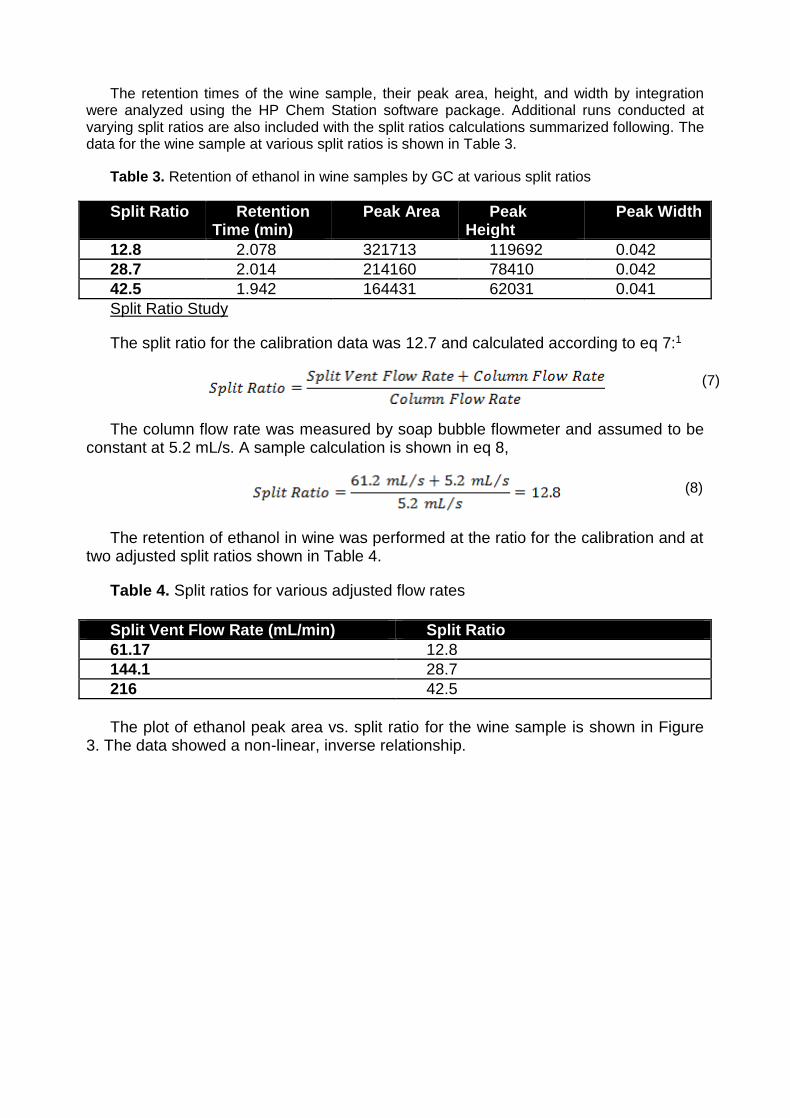
The plot of ethanol peak area vs. split ratio for the wine sample is shown in Figure
3. The data showed a non-linear, inverse relationship.
Split Vent Flow Rate (mL/min) Split Ratio
61.17 12.8
144.1 28.7
216 42.5
(7)
(8)
Figure 3. Ethanol peak area vs. split ratio for wine sample showing a non-linear, inverse decrease in the peak area as the split ratio increases. Coefficient of determination of the model was 1.
Computation of Ethanol Concentration For the external calibration, peak area was chosen for computation of concentration instead
of peak height based on linearity and the lower variance computed in Microsoft Excel. The peak area of the Almaden wine samples was recorded as 321713 for a split ratio of 12.8. This value was used with the computed slope and intercept (eq 4) to determine the concentration of the ethanol in the diluted wine sample with a split ratio matching that of the external calibration. A sample calculation is shown as eq 9.
Accounting for the dilution factors is shown in eq 10 and generates the ethanol concentration in the original sample.
ethanol (v/v)
The uncertainty in the model was calculated according to eq 11 using Microsoft Excel, where m is the number of measurements of the sample, n is the data points, and ysamp is the measured peak area of the sample.
From the calculation in eq 8, 9, and 10 the concentration of the wine was calculated as 13.9±0.2 % ethanol (v/v).
Accuracy of Ethanol Determination in Wine The manufactures reported amount of ethanol in Almaden is 10.0% (v/v). Therefore, the
percent relative error in this ethanol determination is given by eq 12:
(11)
(9)
(10)
A sample calculation is shown in eq 13.
Discussion Questions
The concentration of ethanol in the Almaden wine sample was determined to be 13.9 ± 0.2 % (v/v). The two external standard calibration models produced an excellent fit to the experimental data as evidence by the high value of the linear correlation coefficients which were 0.9999 for peak area and 0.9994 for peak height. The peak area was used for the computation of the concentrations because the variance for the slope and intercept were lower for the peak area in comparison with the height data. The stated concentration of Almaden was 10.0 % (v/v). Wineries have a ±1.5% leeway, so the Almaden was not within the leeway at the 95% confidence interval based on the calibration model.
Given that various class A volumetric pipets were employed in the preparation of the calibration standards from the stock solution and that these concentrations produced a low variance model, it may be the case that the initial production of the 5% (v/v) stock contained less than 5%, thus creating an determinate error resulting in higher calculated values for the wine sample. Without retesting the calibration standards against a second set of standards it is not possible to determine if the error is caused by an initial pipetting error or a lower concentration (sub 100% ethanol) in the reagent used to prepare the 5% stock.
The relationship between the ethanol peak area vs. the split ratio is shown in Figure 3. As the split ratio increased, there was a polynomial decrease in the ethanol peak area. The split ratio is required in GC because the column is 1.2 µm which may result in a saturation of the column and thus column overloading. The split ratio divides the sample flowing into the column by the value determined from eq 7. The less divisions (smaller split ratio), the more concentrated the sample being run through the column. From Figure 3, the ethanol peak area appears to approach an asymptote of 150,000 mV * min peak area as it extends past split ratios of 40. At these increased split ratios, less sample is being introduced into the column which results in lower peak areas and heights. Of note is the reduction in peak width recorded for the highest split ratio. A narrowing of the bands is what we would expect given the larger relative volumes of carrier gas the analyte is exposed to at higher split ratios and is present in the data from table 3. The inverse relationship between the peak area and the split ratio is a result of the proportional decrease in analyte concentration resulting from the split.
References
1. Chemistry 426: Instrumental Analysis Laboratory Manual, Department of
Chemistry, Southern Oregon University: Ashland, OR, 2013; pp 20-28.
(12)
(13)
Mark Weir
Fall 2012
Fractional Distillation
Introduction
The primary focus of the experiment was the isolation of pure samples of cyclohexane and toluene from a supplied 3:2 mixture. Due to relative closeness of boiling points of cyclohexane and toluene, the preferred method for separation proved to be fractional distillation using a packed column. In contrast to simple distillation, the packed column allows varying theoretical plates to be created which exploit the differences between liquid and vapor phases for mixture of two compounds. The plates are the result of multiple vaporization-condensation events which occur when a mixture of two liquids (with different boiling points) pass through a material, allowing the compound with the higher boiling point to condense back to a liquid and return down the column. Adaption of the methods outlined in the procedure can be scaled up to allow for large scale separation of homogenous mixtures of organic solutions.
Procedure
A fractional distillation apparatus was constructed as outlined in figure 1 (attached at the end of this document). All joints were secured to insure that no leaks were present. 25 ml of a supplied 3:2 mixture of cyclohexane to toluene was added to the 50 ml flask which was then placed in the heating mantel. A digital k-style thermometer (0.1 °C precision) was attached to the base of the heating mantel and an alcohol thermometer ( 0.5 °C precision) was placed in the distillation head. A powermite was used to regulate temperature starting with a setting of 3 and slowly increased over time. The distillation head was monitored for reflux ring approach with the temperature setting on the powermite being decreased upon a breach of the distill head – condenser junction. Temperatures at the boiling flask were monitored and kept at apx 126.5 C until a change in still head temperature of 1 °C was observed. All mixtures were collected into graduated cylinders with at least 1ml precision. When still head temperature increased by 1 °C, collection vessels were changed out to allow for isolation of samples. Distillation was carried out until approximately 2 ml of liquid remained in boiling flask. Collected samples where then combined into three theoretical groups, pure cyclohexane, a mixture of cyclohexane & toluene, and pure toluene, based on a recorded graph of distill head temperatures vs ml of collected sample. Finally, the three theoretical separations were run through a gas chromatograph (GC) at the SOU Chemistry lab to check for isolation of cyclohexane and toluene.
Results
The following tables summarize the attached lab data sheet, still head temperature vs. distillate collected graph and gas chromatograph data sheets (all attached to the end of this document).
Fraction –
Sample
Volume
of
Fractio
n (ml)
Temp.
Range of
Collection
(oC)
GC
Retention
Time for
Cyclohexane
(min)
GC
Retention
time for
Toluene
(min)
GC
Normalized
Percent of
Cyclohexane
in Fraction
GC
Normalized
Percent of
Toluene in
Fraction
1 - mw1 10.0 75.5 – 76.5 3.092 3.725 95.88 4.12
2 - mw2 9.0 76.5 –
103.5
3.099 3.784 43.24 56.76
3 - mw3 4.0 103.5 3.110 3.834 1.18 98.82
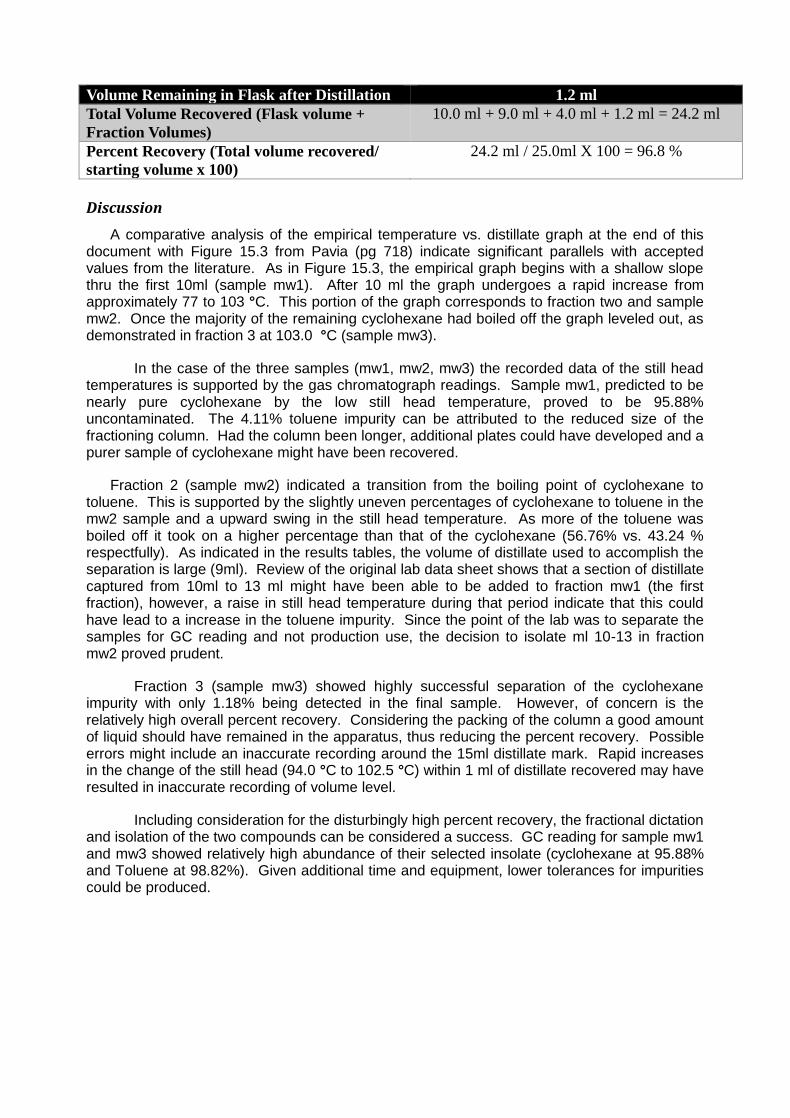
Volume Remaining in Flask after Distillation 1.2 ml
Total Volume Recovered (Flask volume +
Fraction Volumes)
10.0 ml + 9.0 ml + 4.0 ml + 1.2 ml = 24.2 ml
Percent Recovery (Total volume recovered/
starting volume x 100)
24.2 ml / 25.0ml X 100 = 96.8 %
Discussion
A comparative analysis of the empirical temperature vs. distillate graph at the end of this document with Figure 15.3 from Pavia (pg 718) indicate significant parallels with accepted values from the literature. As in Figure 15.3, the empirical graph begins with a shallow slope thru the first 10ml (sample mw1). After 10 ml the graph undergoes a rapid increase from approximately 77 to 103 °C. This portion of the graph corresponds to fraction two and sample mw2. Once the majority of the remaining cyclohexane had boiled off the graph leveled out, as demonstrated in fraction 3 at 103.0 °C (sample mw3).
In the case of the three samples (mw1, mw2, mw3) the recorded data of the still head temperatures is supported by the gas chromatograph readings. Sample mw1, predicted to be nearly pure cyclohexane by the low still head temperature, proved to be 95.88% uncontaminated. The 4.11% toluene impurity can be attributed to the reduced size of the fractioning column. Had the column been longer, additional plates could have developed and a purer sample of cyclohexane might have been recovered.
Fraction 2 (sample mw2) indicated a transition from the boiling point of cyclohexane to toluene. This is supported by the slightly uneven percentages of cyclohexane to toluene in the mw2 sample and a upward swing in the still head temperature. As more of the toluene was boiled off it took on a higher percentage than that of the cyclohexane (56.76% vs. 43.24 % respectfully). As indicated in the results tables, the volume of distillate used to accomplish the separation is large (9ml). Review of the original lab data sheet shows that a section of distillate captured from 10ml to 13 ml might have been able to be added to fraction mw1 (the first fraction), however, a raise in still head temperature during that period indicate that this could have lead to a increase in the toluene impurity. Since the point of the lab was to separate the samples for GC reading and not production use, the decision to isolate ml 10-13 in fraction mw2 proved prudent.
Fraction 3 (sample mw3) showed highly successful separation of the cyclohexane impurity with only 1.18% being detected in the final sample. However, of concern is the relatively high overall percent recovery. Considering the packing of the column a good amount of liquid should have remained in the apparatus, thus reducing the percent recovery. Possible errors might include an inaccurate recording around the 15ml distillate mark. Rapid increases in the change of the still head (94.0 °C to 102.5 °C) within 1 ml of distillate recovered may have resulted in inaccurate recording of volume level.
Including consideration for the disturbingly high percent recovery, the fractional dictation and isolation of the two compounds can be considered a success. GC reading for sample mw1 and mw3 showed relatively high abundance of their selected insolate (cyclohexane at 95.88% and Toluene at 98.82%). Given additional time and equipment, lower tolerances for impurities could be produced.

References
Pavia, Donald L. Introduction to Organic Laboratory Techniques: a Microscale Approach. Belmont, CA: Thomson Brooks/Cole, 2007. Print.
Figure 1 – Diagram of fractional distillation apparatus suggested by Pavia (source, Pavia, 2004)
Mark Weir and Jerad Harris 15 March 2013
A Comparison of Fatty Acids Isolated from the Triglycerides of Grain-Fed and
Grass-Fed Beef
Abstract
Fatty acid profiles for grass and grain-fed beef were analyzed by GC-MS to determine
ratios and composition of saturated fatty acids (SFA) and unsaturated fatty acids (UFA). Grass-fed beef was found to have higher average percentages of SFA (59.06% vs. 52.88%) including higher stearic acid composition (20.72% vs. 29.67). Vaccenic acid, a UFA precursor conjugated linoleic acid was found only in grass fed samples (3.06%). Omega-3 to 6 ratios, an important nutritional bench mark, were found to be 1:3.47 in grass-fed beef and 1:7.6 in grain-fed with one grain fed sample containing no omega-3 UFA. Taken collectively, it was determined that the grass-fed beef contained a healthier profile of fatty acids.
Introduction
Recently a litany of claims have been made by select beef producers and natural food enthusiasts claiming grass-fed beef is inherently healthier than meat from grain-fed cattle1. These claims are buttressed by numerous scientific studies which support a host of potential benefits ranging from decreased cardiac arrest2, increased anti-oxidative capacity3 and anit-carcinogenic properties4. So extensive are the purported benefits that numerous scientific review articles have been dedicated to the subject5. As summarized by Daley et. al. the increased nutrition value of grass-fed beef stems from improved complexity of fatty acids (FA) found in the meat. Conjugated Linoleic Acid (CLA), trans vaccenic acid (TVA), and omega-3 (n-3) FA have all been demonstrated to be higher in grass-fed beef and increased ratios of each are considered to have positive heath benefits5.
Before discussing the importance of the FA classes CLA, TVA and n-3, it is valuable to cover the common saturated fatty acids (SFA) found in beef. As noted by Daley et. al., there is little difference reported in the total SFA content observed in cattle between grass and grain-fed. There is however clear indications that grain-fed beef contains higher relative levels of lauric (C12:0), myristic (C14:0) and palmitic (C16:0) acids. These three SFA are significant - as compared to stearic acid (C18:0), another SFA – in that higher ratios of each (or all) have been linked to increases in low-density-lipoprotein (LDL) cholesterol which ultimately results in increased incidences of cardiovascular disease (CVD). By contrast, the fore mentioned stearic acid does not appear to have adverse effects on cholesterol concentrations. Thus elevated concentrations of stearic acid, relative to the total SFA, can provide a source of significant metabolic energy sans undesirable side effects. Elevated levels of arachidic acid (C20:0), a long SFA, have been shown to induce prolonged inflammatory response, however most studies show only limited quantities of the FA in beef (less than 0.25% of total fat by weight).5, 6
As alluded to previously, unsaturated fatty acids (UFA) can play a diverse role in metabolic well-being. Numerous studies have shown that increased concentrations of UFA -particularly poly UFA (PUFA) - consumed as part of a steady caloric diet, can reduce chances of death resulting from CVD5. Grass-fed samples have been show to contain TVA which are valuable for their high conversion within humans (19% to 30%) to CLA7. Conjugated linoleic acid, has experienced two decades of extensive study with research linking heighted levels to decreased risk of hardening of the heart, cancer and diabetes.

The ratio of Omega-3 to Omega-6 fatty acids has also been shown to correlate to better health. Specifically, increasing the amount of n-3 to bring its ratio to approximately ¼ of n-6 more closely aligns it with dietary needs. Two essential components of human metabolism are α-linolenic acid (αLA, a n-3 FA) and linoleic acid (LA, a n-6 FA), found to be in a more balanced ratio in grass verses grain-fed beef5. These FA must be consumed in the diet and are important primary metabolites, undergoing elongation and specialization in the human body.
While it is clear that increased levels of TVA, αLA, LA and other PUFA have potential benefits, the quantification of each requires separation and identification of the FA profile. Presented here is the comparative examination of lipid profiles for two beef samples, one grass-fed and one grain-fed. Following isolation, saponification (the cleaving of the individual fatty acids from the triglyceride) and methylation of the fatty acid, Gas Chromatography-Mass Spectrometry (GC-MS) was employed to identify the associated fatty acid profiles. It was initially hypothesized that that grass-fed beef would contain a more complex assemblage of fatty acids and have higher ratios of CLA, TVA and lower frequencies of myristic and palmitic fatty acids with higher ratios of n-3 to n-6 omegas.
Experimental
Chemicals Beef samples were collected from a local supplier (Cherry Creek Meats,
Medford, OR) and consisted of two grades, grass-fed bovine and grain-fed bovine. Initial samples consisted of quantities as described in Table 1:
Table 1. Beef Sample Feed Type and Initial Sample Weight
Sample Number Type of Beef Weight (grams)
Sample 1 Grain-Fed 20.0007
Sample 2 Grain-Fed 20.1167
Sample 3 Grass-Fed 20.0400
Sample 4 Grass-fed 20.8733
40 mL of 2 M Potassium Hydroxide (KOH) was prepared in a 50% methanol: water (CH4O:H2O) solution. Methanol (MeOH), Chloroform (CHCl3), Acetone (C2H6O) and Boron trifluoride-methanol (BF3-MeOH) were all of laboratory grade.
Isolation of Triglycerides Beef samples were individually homogenized in a minimal amount of MeOH
(apx 20mL) and the contents were separated and mixed with a 2:1 chloroform:MeOH solution (60mL:30mL) before being purified through Whatman #3 filter paper via vacuum filtration. Solvated triglycerides were transferred to a Buchi Rotavapor under vacuum and evaporated to the consistency of viscous oil (apx 2mL).
Recrystallization of Unknown Lipids Oil and residue condensed by the Rotavapor were dissolved in 30 mL of warm
acetone and 10 mL of MeOH. All solids were allowed to dissolve and the contents were covered and transferred to a freezer over night to induce crystallization. The supernate was removed by vacuum filtration using Whatman 42 filter paper and the crystals were twice washed with 10 mL aliquots of Acetone (cold).
Saponification of Triglycerides from Fatty Acid Analysis Crystal samples as indicated in table 2 were mixed with 5 mL of 2 M KOH (50%
MeOH as described earlier) in a small conical test tube.
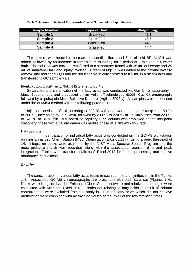
Table 2. Amount of Isolated Triglyceride Crystal Subjected to Saponification
Sample Number Type of Beef Weight (mg)
Sample 1 Grain-Fed 41.1
Sample 2 Grain-Fed 45.7
Sample 3 Grass-Fed 44.0
Sample 4 Grass-fed 44.4
The mixture was heated in a steam bath until uniform and 5mL of cold BF3-MeOH was added, followed by an increase in temperature to boiling for a period of 3 minutes in a water bath. The solution was cooled, transferred to a separatory funnel with 25 mL of hexane and 25 mL of saturated NaCl and lightly inverted. 1 gram of MgSO4 was added to the hexane layer to remove any additional H2O and the solutions were concentrated to 0.5 mL in a steam bath and transferred to GC sample vials.
Identification of Fatty Acid Methyl Esters using GC-MS Separation and identification of the fatty acids was conducted via Gas Chromatography –
Mass Spectrometry and processed on an Agilent Technoloiges 6890N Gas Chromatograph, followed by a qudrapole Mass Selective Detector (Agilent 5973N). All samples were processed under the auto454 method with the following parameters:
Injection consisted of 1µL, entering at 200 °C with and oven temperature ramp from 50 °C to 200 °C, increasing by 25 °C/min, followed by 200 °C to 220 °C at 1 °C/min, then from 220 °C to 240 °C at 10 °C/min. A fused-silica capillary HP-5 column was employed as the non-polar stationary phase with a helium carrier gas mobile phase at 1.7mL/min flow-rate.
Data analysis Identification of individual fatty acids was conducted on the GC-MS workstation
running Enhanced Chem Station (MSD Chemstation E.02.01.1177) using a peak threshold of 14. Integration peaks were examined by the NIST Mass Spectral Search Program and the most probable match was recorded along with the associated retention time and peak integration. Tables were transfer to Microsoft Excel 2013 for further processing and relative abundance cacualtions.
Results
The concentration of various fatty acids found in each sample are synthesized in the Tables
1-4. Associated GC-MS chromatographs are presented with each data set (Figures 1-4). Peaks were integrated via the Enhanced Chem Station software and relative percentages were calculated with Microsoft Excel 2013. Peaks not relating to fatty acids (a result of column contaminates) were excluded from the analysis. Further, fatty acids which did not achieve methylation were combined with methylated values at the lower of the two retention times.
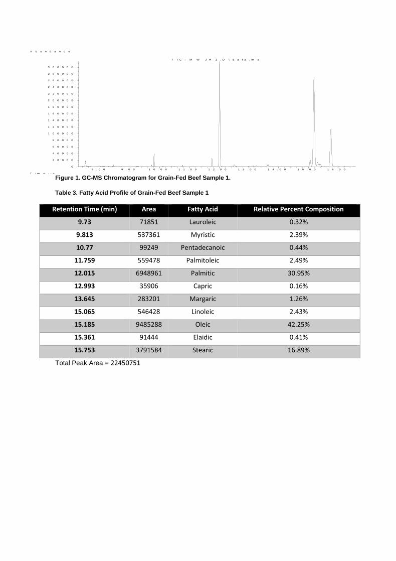
Figure 1. GC-MS Chromatogram for Grain-Fed Beef Sample 1.
Table 3. Fatty Acid Profile of Grain-Fed Beef Sample 1
Retention Time (min) Area Fatty Acid Relative Percent Composition
9.73 71851 Lauroleic 0.32%
9.813 537361 Myristic 2.39%
10.77 99249 Pentadecanoic 0.44%
11.759 559478 Palmitoleic 2.49%
12.015 6948961 Palmitic 30.95%
12.993 35906 Capric 0.16%
13.645 283201 Margaric 1.26%
15.065 546428 Linoleic 2.43%
15.185 9485288 Oleic 42.25%
15.361 91444 Elaidic 0.41%
15.753 3791584 Stearic 16.89%
Total Peak Area = 22450751
8 . 0 0 9 . 0 0 1 0 . 0 0 1 1 . 0 0 1 2 . 0 0 1 3 . 0 0 1 4 . 0 0 1 5 . 0 0 1 6 . 0 00
2 0 0 0 0
4 0 0 0 0
6 0 0 0 0
8 0 0 0 0
1 0 0 0 0 0
1 2 0 0 0 0
1 4 0 0 0 0
1 6 0 0 0 0
1 8 0 0 0 0
2 0 0 0 0 0
2 2 0 0 0 0
2 4 0 0 0 0
2 6 0 0 0 0
2 8 0 0 0 0
3 0 0 0 0 0
T i m e - - >
A b u n d a n c e
T I C : M W J H 1 . D \ d a t a . m s
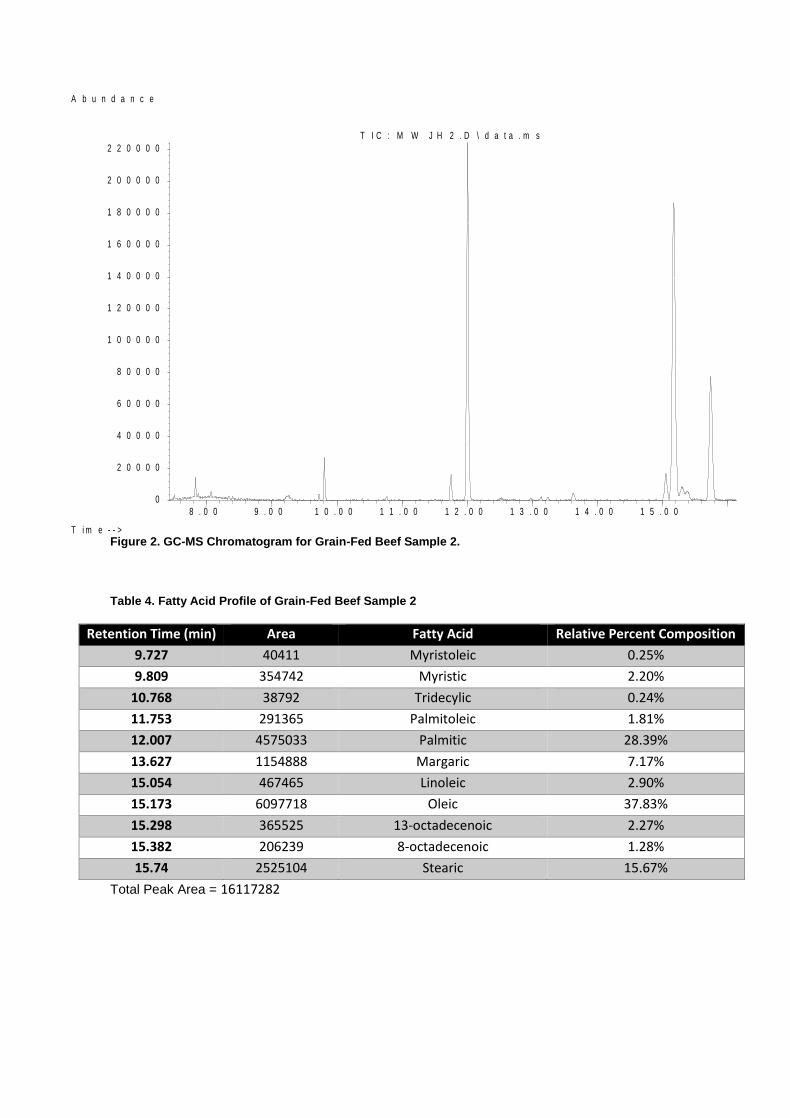
Figure 2. GC-MS Chromatogram for Grain-Fed Beef Sample 2.
Table 4. Fatty Acid Profile of Grain-Fed Beef Sample 2
Retention Time (min) Area Fatty Acid Relative Percent Composition
9.727 40411 Myristoleic 0.25%
9.809 354742 Myristic 2.20%
10.768 38792 Tridecylic 0.24%
11.753 291365 Palmitoleic 1.81%
12.007 4575033 Palmitic 28.39%
13.627 1154888 Margaric 7.17%
15.054 467465 Linoleic 2.90%
15.173 6097718 Oleic 37.83%
15.298 365525 13-octadecenoic 2.27%
15.382 206239 8-octadecenoic 1.28%
15.74 2525104 Stearic 15.67%
Total Peak Area = 16117282
8 . 0 0 9 . 0 0 1 0 . 0 0 1 1 . 0 0 1 2 . 0 0 1 3 . 0 0 1 4 . 0 0 1 5 . 0 0
0
2 0 0 0 0
4 0 0 0 0
6 0 0 0 0
8 0 0 0 0
1 0 0 0 0 0
1 2 0 0 0 0
1 4 0 0 0 0
1 6 0 0 0 0
1 8 0 0 0 0
2 0 0 0 0 0
2 2 0 0 0 0
T i m e - - >
A b u n d a n c e
T I C : M W J H 2 . D \ d a t a . m s
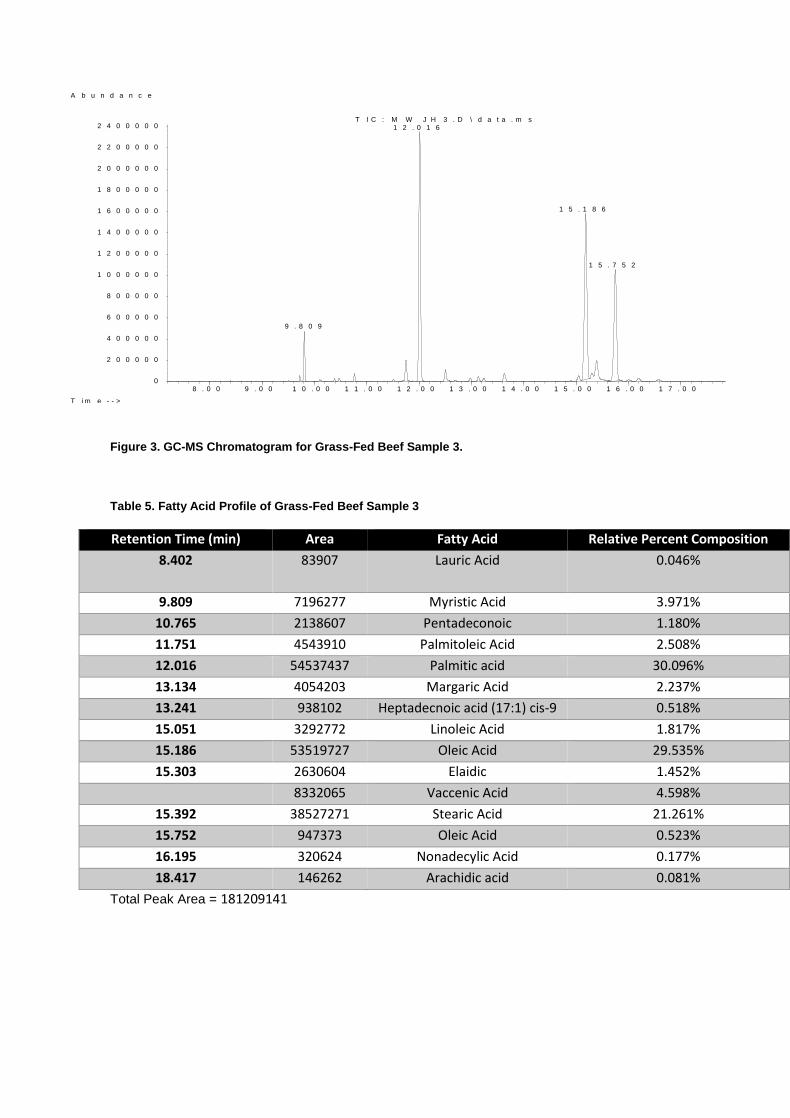
Figure 3. GC-MS Chromatogram for Grass-Fed Beef Sample 3.
Table 5. Fatty Acid Profile of Grass-Fed Beef Sample 3
Retention Time (min) Area Fatty Acid Relative Percent Composition
8.402 83907 Lauric Acid 0.046%
9.809 7196277 Myristic Acid 3.971%
10.765 2138607 Pentadeconoic 1.180%
11.751 4543910 Palmitoleic Acid 2.508%
12.016 54537437 Palmitic acid 30.096%
13.134 4054203 Margaric Acid 2.237%
13.241 938102 Heptadecnoic acid (17:1) cis-9 0.518%
15.051 3292772 Linoleic Acid 1.817%
15.186 53519727 Oleic Acid 29.535%
15.303 2630604 Elaidic 1.452%
8332065 Vaccenic Acid 4.598%
15.392 38527271 Stearic Acid 21.261%
15.752 947373 Oleic Acid 0.523%
16.195 320624 Nonadecylic Acid 0.177%
18.417 146262 Arachidic acid 0.081%
Total Peak Area = 181209141
8 . 0 0 9 . 0 0 1 0 . 0 0 1 1 . 0 0 1 2 . 0 0 1 3 . 0 0 1 4 . 0 0 1 5 . 0 0 1 6 . 0 0 1 7 . 0 00
2 0 0 0 0 0
4 0 0 0 0 0
6 0 0 0 0 0
8 0 0 0 0 0
1 0 0 0 0 0 0
1 2 0 0 0 0 0
1 4 0 0 0 0 0
1 6 0 0 0 0 0
1 8 0 0 0 0 0
2 0 0 0 0 0 0
2 2 0 0 0 0 0
2 4 0 0 0 0 0
T i m e - - >
A b u n d a n c e
T I C : M W J H 3 . D \ d a t a . m s
9 . 8 0 9
1 2 . 0 1 6
1 5 . 1 8 6
1 5 . 7 5 2
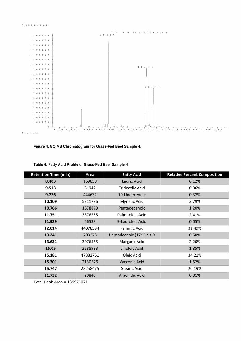
Figure 4. GC-MS Chromatogram for Grass-Fed Beef Sample 4.
Table 6. Fatty Acid Profile of Grass-Fed Beef Sample 4
Retention Time (min) Area Fatty Acid Relative Percent Composition
8.403 169858 Lauric Acid 0.12%
9.513 81942 Tridecylic Acid 0.06%
9.726 444632 10-Undecenoic 0.32%
10.109 5311796 Myristic Acid 3.79%
10.766 1678879 Pentadecanoic 1.20%
11.751 3376555 Palmitoleic Acid 2.41%
11.929 66538 9-Lauroleic Acid 0.05%
12.014 44078594 Palmitic Acid 31.49%
13.241 703373 Heptadecnoic (17:1) cis-9 0.50%
13.631 3076555 Margaric Acid 2.20%
15.05 2588983 Linoleic Acid 1.85%
15.181 47882761 Oleic Acid 34.21%
15.301 2130526 Vaccenic Acid 1.52%
15.747 28258475 Stearic Acid 20.19%
21.732 20840 Arachidic Acid 0.01%
Total Peak Area = 139971071
8 . 0 0 9 . 0 0 1 0 . 0 0 1 1 . 0 0 1 2 . 0 0 1 3 . 0 0 1 4 . 0 0 1 5 . 0 0 1 6 . 0 0 1 7 . 0 0 1 8 . 0 0 1 9 . 0 0 2 0 . 0 0 2 1 . 0 0
0
1 0 0 0 0 0
2 0 0 0 0 0
3 0 0 0 0 0
4 0 0 0 0 0
5 0 0 0 0 0
6 0 0 0 0 0
7 0 0 0 0 0
8 0 0 0 0 0
9 0 0 0 0 0
1 0 0 0 0 0 0
1 1 0 0 0 0 0
1 2 0 0 0 0 0
1 3 0 0 0 0 0
1 4 0 0 0 0 0
1 5 0 0 0 0 0
1 6 0 0 0 0 0
1 7 0 0 0 0 0
1 8 0 0 0 0 0
1 9 0 0 0 0 0
T i m e - - >
A b u n d a n c e
T I C : M W J H 4 . D \ d a t a . m s
1 2 . 0 1 4
1 5 . 1 8 1
1 5 . 7 4 7

Table 7.Saturated and Unsaturated Fat Content for Grain-Fed Beef Sample 1
Saturated Fats Relative Percentage Unsaturated Fats Relative Percentage
Myristic 2.39% Lauroleic 0.32%
Pentadecanoic 0.44% Palmitoleic 2.49%
Palmitic 30.95% Linoleic 2.43%
Capric 0.16% Oleic 42.25%
Margaric 1.26% Elaidic 0.41%
Stearic 16.89% -- --
Total Saturated Fats 52.10% Total Unsaturated Fats 47.90%
Table 8. Saturated and Unsaturated Fat Content for Grain-Fed Beef Sample 2
Saturated Fats Relative Percentage Unsaturated Fats Relative Percentage
Myristic 2.20% Myristoleic 0.25%
Tridecylic 0.24% Palmitoleic 1.81%
Palmitic 28.39% Linoleic 2.90%
Margaric 7.17% Oleic 37.83%
Stearic 15.67% 13-octadecenoic 2.27%
-- -- 8-octadecenoic acid 1.28%
Total Saturated Fats 53.66% Total Unsaturated Fats 46.34%
Table 9. Saturated and Unsaturated Fat Content for Grass-Fed Beef Sample 3
Saturated Fats Relative Percentage Unsaturated Fats Relative Percentage
Lauric 0.05% Palmitoleic 2.51%
Myristic 3.97% Heptadecnoic (17:1) cis-9
0.52%
Pentadecanoic 1.18% Linoleic 1.82%
Palmitic 30.10% Oleic 30.06%
Margaric 2.24% Elaidic 1.45%
Stearic 21.26% Vaccenic 4.60%
Nonadecylic 0.18% -- --
Arachidic 0.08% -- --
Total Saturated Fats 59.05% Total Unsaturated Fats 40.95%
Table 10. Saturated and Unsaturated Fat Content for Grass-Fed Beef Sample 4
Saturated Fats Relative Percentage Unsaturated Fats Relative Percentage
Lauric 0.12% Palmitoleic 2.41%
Tridecylic 0.06% 9-Lauroleic 0.05%
Myristic 3.79% Heptadecanoic (17:1) cis-9
0.50%
Pentadecanoic 1.20% Linoleic 1.85%
Palmitic 31.49% Oleic 34.21%
Margaric 2.20% Vaccenic 1.52%
Stearic 20.19% -- --
Arachidic 0.01% -- --
Total Saturated Fats 59.07% Total Unsaturated Fats 40.62%
Table 11. Composition of the Four Samples Comparing Degree of Saturation
Sample Monounsaturated Polyunsaturated Unsaturated Saturated
Grain (1) 45.47% 2.43% 47.90% 52.10%
Grain (2) 43.44% 2.90% 46.34% 53.66%
Grass (1) 38.19% 2.35% 40.54% 59.07%
Grass (2) 39.13% 2.33% 40.95% 59.05%
Table 12. Composition of Four Samples Comparing Omega 3,6,9
Sample Omega-3 Omega-6 Omega-9 Trans
Grain (1) 0.32% 2.43% 42.25% 0.41%
Grain (2) -- 2.90% 37.83% --
Grass (1) 0.52% 1.82% 30.06% 6.05%
Grass (2) 0.55% 1.85% 34.21% 1.52%
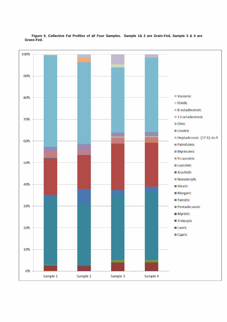
Figure 5. Collective Fat Profiles of all Four Samples. Sample 1& 2 are Grain-Fed, Sample 3 & 4 are Grass-Fed.
Discussion
As described by Daley et. al., quantifying the health benefits of grass verse grain fed beef requires more than a simple quantification of individual fats from one sample with those of another. A holistic profile of the fat content provides a better overall picture of the potential heath benefits of one feeding regiment over another. However, by comparing relative percentages and types of SFA, PUFA, n-3 and n-6 FA it is possible to deliver a broad stroke assessment. Based on the data it appears that the grass fed beef is characteristically healthier.
In contrast to previous reporting that claimed little difference between total SFA content of grass and grain fed cattle, our results indicate grass fed beef containing an average of 6.18% more SFA than grain fed beef (average total saturated, grass=59.06%, grain=52.88%). Consistent with the work of others, the grass fed beef displayed increased concentrations of stearic acid as a portion of total SFA (4.45% higher on average in grass vs grain fed). However, this did not translate into a reduction in palmitic, myristic or lauric FA, with palmitic quantities nearly identical, increases in myristic in the grass fed and the presence of trace amounts of lauric only found in grass fed samples (sample 3=0.05%, sample 4=0.12%). Higher levels of lauric and myristic acid have been linked to increased cholesterol and indicates that these grass fed samples may have a higher potential for causing some forms of CVD5.
Both grass-fed samples contained significant levels of vaccenic acid (sample 3=4.60%, sample 4=1.52%). This important precursor to beneficial CLA is conspicuously absent from both of the grain fed samples. Given the multiple health benefits derived from CLA, any comparison of meats containing or lacking the FA favors the former as the more salubrious.
The presence of the UFA, Heptadecanoic (17:1) cis-9 in the two grass samples is both noteworthy and exciting as its incidence is often unreported in the literature7. Heptadecnoic (17:1) cis-9 is the byproduct of the breakdown of linoleic and linolenic FA by microorganism in the gut of cattle8. It can be speculated that the presence in the grass-fed beef (and absence in grain-fed) is indicative of a more complex biota in the gut of grass-fed cows. Since a purported benefit of grass-fed beef is increased concentrations of novel fatty acids - especially monoenoics such as Heptadecnoic (17:1) cis-9 - its presence boosts the claim that grass-fed beef have higher potential for conjugated linoleic acid production.
Sample 3 (grain-fed) contained the interesting unsaturated fat elaidic acid in relatively high amounts (1.452% of total fat for that sample). Elaidic acid is an 18 carbon transfat (with the double bond occurring at the 9 carbon) and has been found in some meats but has been primarily associated with the milk of cows9. Elaicd Acid is of interest because it has been linked to additional activity in the cholesterylester transfer protein resulting in increases in VLDL and decreases in HDL10. The presence of elaidic acid in the grain and grass sample acts to both support and refute the potential health claims as elaidic acid might also be a precursor to CLA.
Over all, the profile for samples 3 and 4 (grass-fed) contain an increased complexity of fatty acids. Additionally, omega-3 to 6 ratios was increased in the grass-fed to 0.28 and 0.29 for samples 3 and 4. Grain-fed sample 1 had a ratio of only 0.13 and sample 2 displayed no n-3 FA. Combined with the presence of vaccenic FA (natural trans-fat), the grass-fed samples can be said to have a healthier fat profile. It should not go without note that the grass fed samples did contain elevated SFA which may result in higher LDL, however, given the overwhelming positive benefits of LCA and its precursors, the grass-fed beef is clearly a better choice.
References
Pollan, M. 2002. This Steer’s life. The New York Times Magazine, March 31: pg 44
Siscovick, D. S; Raghunathan, T. E. Dietary Intake and Cell Membrane Levels of Long-Chain
n-3 Polyunsaturated Fatty Acids and the Risk of Primary Cardiac Arrest. JAMA 1995, 274(17),
1363-1367.
Lopez-Bote, C. J.; R.Sanz Arias, A.I;. Rey, A;. Castano, B.; Isabel, J;. Effect of free-range
feeding on omega-3 fatty acids and alpha-tocopherol content and oxidative stability of eggs.
Animal Feed Science and Technology 1998, 72, 33-40.
Ip, C; Scimeca J.A. Conjugated linoleic acid. A powerful anti-carcinogen from animal fat
sources. Cancer 1994, 74, 1050-1054.
Daley, C. A.; Abbott, A; Doyle, P. S.; Nader, G. A.; Larson, S. A review of fatty acid profiles
and antioxidant content in grass-fed and grain-fed beef. Nutrition Journal 2010, 9, 1-12.
Adam, O;, Beringer C; Kless T; Lemmen C; Adam A; Wiseman M; Adam P; Klimmek R;
Forth W. Anti-inflammatory effects of a low arachidonic acid diet and fish oil in patients with
rheumatoid arthritis. Rheumatol Int. 2003, 3, 27-36.
Turpeinen, A.M.; Mautanen, M.; Aro, A.; Salminen, I.; Basu, S.; Palmquist, D.L. Bioconversion
of vaccenic acid to conjugated linoleic acid in humans. American Journal of Clinical Nutrition
2002, 75,504-10.
Alves, S.P.; Marcellno, C.; Portugal, P. V.; Bessa, J. B. Short Communication: The Nature of
Heptadecenoic Acid in Ruminant Fats. J. Dairy Sci. 2005, 89, 170-173
Alonson, L.; Fontecha, J.; Lozada, L; Fraga, M.J.; Juarez, M. Fatty acid composition of caprine
milk: major, brached-chaing and trans fatty acids. J. Dairy Sci. 1999, 82, 878-884.
Abbey. M.; Nestel, P. J. Plasma cholesteryl ester transfer protein activity is increased when
trans-elaidic acid is substituted for cis-oleic acid in the diet. Atherosclerosis, 1994, 106, 99–
107.
Mark Weir and Jerad Harris 1 March 2013
Sequence Determination of an Unknown Dipeptide
Abstract
The sequence of an unknown dipeptide was determined to be alanine (Ala) and leucine
(Leu). Nuclear Magnetic Resonance experiments, specifically, Proton (1H), Carbon 13 (13C), Distortionless Enhancement by Polarization Transfer (DEPT-135) and Correlation Spectroscopy (COSY), reveled 9 nonequivalent carbons and 15 total protons. The dipeptide was processed by way of the Edman degradation, pre and post hydrolzation, and the products were separated and compared against known standards using High-Performance Liquid Chromatography. Final determination of the dipeptide sequence was confirmed by COSY experiment and is reported to be N-Ala-Leu-C.
Introduction
Dipeptides represent the simplest form of protein, consisting of two amino acids joined covalently by dehydration. While considerably simpler when compared to enzymes and megaynthetases - which can contain tens, hundreds or even thousands of amino acids11 - dipeptides play a number of important biochemical functions. Perhaps one of the most notorious dipeptides is the artificial sweater aspartame, composed of the amino acids, aspartic acid and phenylalanine. This dipeptide is employed throughout the food industry as a low calorie alternative to sugar. In numerous biochemical reactions, dipeptides act as cofactors, inhibitors and primary metabolites. Examples of important antioxidant dipeptides in animals include, Carnosine, Anserine and Homoanserine which can be found as components of the brain and muscle12,13. Dipeptides also make for a powerful teaching tools for the aspiring biochemist in that they are relatively easy to identify via Nuclear Magnetic Resonance (NMR) or the Edmand system of derivation followed by subsequent analysis with High-Performance Liquid Chromatography (HPLC).
Nuclear Magnetic Resonance (NMR) provides one powerful approach for identifying unknown dipeptides. Through comparison of proton (1H), carbon-13 (13C), Distortionless Enhancement by Polarization Transfer (DEPT-135) and Correlation Spectroscopy (COSY) experiments it is possible to determine the structural location and orientation of atoms making up a dipeptide. The NMR technique utilizes magnetically induced spin state transitions and resulting emission spectra (the product of radio wave bombardment) to identify atoms having varying molecular environments. Given the relatively small size of dipeptides (>400 daltons), NMR is exceedingly informative, allowing the solving of the individual locations of atoms within the compound. Of special use in solving such problems is the COSY experiment which associates atoms within the molecule and allows for specification of which protons are near which other protons. Although a powerful tool for deciphering relatively small molecules, NMR requires extensive computation as molecules increase in size and begin to experience secondary and tertiary folding. For this reason it can be advantageous to pluck individual amino acids off of a terminal end of a peptide for examination. A commonly employed technique for the removal and identification of individual amino acids is the Edman procedure.
The Edman procedure (also known as Edman degradation) was first developed by Pehr Edman in 1950 for the cleavage of N terminal amino acids from peptides14. The process begins by attaching phenylilisothiocyanate (PITC), colloquially referred to as Edaman’s reagent, to the exposed N terminal of a peptide (in this case, the dipeptide of interest) using triethylamine (TEA) as a catalyzing weak organic base. The resulting phenylthiocarbamyl peptide is subjected to heating and treatment with a concentrated acid, inducing a cleavage of the terminal peptide bond as a result of a nucleophilic attack by the nitrogen of PITC on the
carbonyl of the bond. The ring closure produces an anilinothiazolinone, which, composed of the N terminal and R group of the amino acid of interest, is reacted with acid to convert it from phenylthiocarbamyl (PTC) to phenylthiohydantion (PTH). The derivatized product can then be tested against know standards and, based on comparison of retention times, uniquely distinguished. The Edman procedure has the added benefit of allowing for the remaining peptide to be reprocessed and thus, one by one, individual amino acids can be cleaved, derivatized and identified. The procedure is however limited in that peptides in excess of 50 units produce undesirable side products when processed. As such, larger proteins must be first deconstructed to acceptable length before being reacted.
The separation and thus identification of PTH-derivatives requires that the individual biomolecules are isolated based on their respective chemistry. Various forms of chromatography monitored by a detector allow for cleaved amino acids to be compared with known standards. While flame ionization detector gas chromatography and gas chromatography coupled mass spectroscopy both provide acceptable separation of many biomolecules, they do a poor job of separating PTH derivatives and have the added disadvantage of being destructive to the compound15. For this reason, High-Performance Liquid Chromatography (HPLC) is the preferred instrumentation for the identification of PTH derivatives. HPLC, similar to all chromatography, consist of a stationary phase (packed in a column) and a mobile carrier phase. In the case of HPLC, the carrier phase is a liquid solvent and can often consist of multiple liquid phases which can be applied in gradients to produce additional separation of the analyte(s) of interest. By adjusting the polarity, pressure and size of the mobile and stationary phases, it is possible to optimize HPLC procedures to be highly selective. As compounds leave the HPLC they pass through an ultra violet or infra-red detector which confirms the presence of the desired compound (and can often provide quantification). Combined with Edman degradation and known standards, HPLC provides a rapid and effective method for determining peptide sequences.
Presented here is the identification of an unknown dipeptide by NMR and Edman protein sequencing followed by separation using HPLC. To reduce Prozac dependence among fledging biochemistry students, only nine of the twenty genetically coded for amino acids were candidates for inclusion in the dipeptide. Additionally, the dipeptide was pre identified as not being a homodimer such as Alanine-Alanine or Valine-Valine. The nine possible amino acids, listed alphabetically were, Alanine (Ala), Glycine (Gly), Histidine (His), Isoleucine (Ile), Leucine (Leu), Methionine (Met), Proline (Pro), Serine (Ser), and Valine (Val). Proton, carbon, DEPT-135 and COSY NMR experiments were all employed to develop a model of the chemical environment of the dipeptide’s constitutes. Edman procedure and HPLC provide a mechanism for the confirmation of findings from the NMR experiment and provided introduction and familiarization with the process and instrumentation.
Experimental
Chemicals An unknown dipeptide, labeled “E”, was supplied by the Southern Oregon University chemistry department in a solid form (~11 gm) and as a separate, predissolved (90% H2O, 10% D2O solvent), NMR sample. Ethanol (EtOH, C2H6O), triethylamine (TEA, C6H15N), phenylisothiocyanate (PITC, C7H5NS), heptane, ethyl acetate, 12 M HCl, glacial acetic acid, and acetonitrile used throughout the experiment where all of laboratory grade. In cases where H2O was utilized, it was distilled. HPLC grade acetronitrile (NH4C2H3O2) and H2O were used where appropriate.
NMR Initial quantification of number of proton and carbon as well as structural data for the sample (unknown E) was acquired by NMR spectroscopy. Spectrums were acquired on a Bruker 400 UltraShield running the TOPSPIN 3.1 software package. Initial proton NMR (1H) was conducted on a spinning sample after solvent suppression of the H20 peak at 4.73 ppm. Power level nine was set to 55 with an o1 value of 2893.61 Hz. Duration was set to 2 seconds for 8 scans. For the carbon 13C, a solvent selection of D2O was applied to the instrument software and the number of scans was increased to 64. For the DEPT-135 experiment, D2O was again selected as a solvent and the rga command was used for automated gain adjustment. The COSY (1H) experiment involved a number of specialized parameter changes. The PULPROG command was used to adjust the following settings, 01 was changed to 2893.61 (Hz), pL 9 was changed to 55.00 and d1 was changed to 2.00. Data was processed as described in the data analysis section.
Dipeptide PTH derivation Derivation of the intact dipeptide was completed by dissolving 5.5 mg of unknown E in 600 µL of 80% EtOH, 140 µL TEA, and 100 µL PITC. The solution was heated at a constant 55 ºC for 30 minutes. Upon removal from heat, 1 mL of 2:1 heptane:ethyl acetate (HE) was added and the solution was thoroughly mixed. The HE layer was removed and a second washing was conducted with an additional 1 mL of HE mixture. The HE layer was again removed and discarded and the aqueous phase was placed under vacuum with slight air inclusion for a period of 24 hours to dry. Cleavage of the PTC-dipeptide product was conducted by adding 1 mL of concentrated HCl (12 M) to the dried compound and heating for 10 minutes in a water bath, again at 55 ºC. The solvent (including HCl) was then removed by evaporation under vacuum for 24 hours. The compound was extracted by adding 500 µL of H20 and 500 µL ethyl acetate. The mixture was stirred, allowed to rest and the ethyl acetate layer was set-aside. A second washing with an additional 500 µL ethyl acetate was conducted and the two extractions were combined and dried via the method described previously. Finally, the PTC byproduct was converted to a PTH-derivative through the addition of 1 mL of a 2:1 mixture of glacial acetic acid:4 M HCl. The sample was heated for 45 minutes in the water bath described above and evaporated under heat and vacuum, yielding the PTH-amino acid derivative. Equal parts of acetonitrile and H2O (500 µL each) were added to the dry solid and stored until HPLC analysis.
Dipeptide cleavage and residual PTH derivation The remaining 5.5 mg of unknown dipeptide E were hydrolyzed and converted as follows. The dipeptide was dissolved in 6 M HCl (100 µL) and transferred to a glass tube which had been flame sealed at one end. Once filled, the open end of the tube was also flame sealed and the sample was placed in an oven (100 ºC) for 17 hours. The fluid was removed from the glass tube and all water was evaporated off. The sample was washed with 0.1 mL of H2O and again evaporated to dryness. PTH-derivtization was accomplished by adding 100 µL of H2O, 500 µL of 95% EtOH, 140 µL of TEA and 100 µL PITC. The solution was heated for 30 minutes at 55 ºC. Washing, coupling extraction and conversion were performed as previously described with the exception that the sample did not require cleavage or further extraction.
HPLC Analysis HPLC analysis was conducted at the SOU instrument lab on the HP 1100 HPLC using a C18 reverse phase, 215mm column. Ala, Leu and Ile PTH amino acid standards were selected based on the results from NMR data. One (1) mg of Ala and Ile were dissolved in one sample and 1 mg of Leu was dissolved in a second, each containing 1 mL of 1:1 HPLC grade C2H3N:H2O. A gradient of the two solvents, A) 10% C2H3N, 90% 17 mM NH4C2H3O2 and B) 90% C2H3N, 10% 17 mM NH4C2H3O2, was applied, as depicted in Table 1, to separate the samples. The solution of 17mM NH4C2H3O2 was filtered to remove possible impurities. Detector signals were taken at wavelengths of 254.4 nm, 215.4 nm and 280.4 nm.
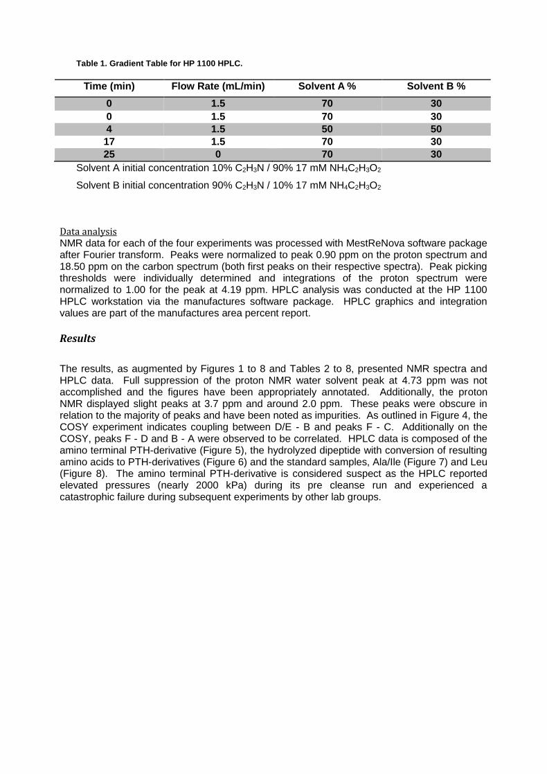
Table 1. Gradient Table for HP 1100 HPLC.
Time (min) Flow Rate (mL/min) Solvent A % Solvent B %
0 1.5 70 30
0 1.5 70 30
4 1.5 50 50
17 1.5 70 30
25 0 70 30
Solvent A initial concentration 10% C2H3N / 90% 17 mM NH4C2H3O2
Solvent B initial concentration 90% C2H3N / 10% 17 mM NH4C2H3O2
Data analysis NMR data for each of the four experiments was processed with MestReNova software package after Fourier transform. Peaks were normalized to peak 0.90 ppm on the proton spectrum and 18.50 ppm on the carbon spectrum (both first peaks on their respective spectra). Peak picking thresholds were individually determined and integrations of the proton spectrum were normalized to 1.00 for the peak at 4.19 ppm. HPLC analysis was conducted at the HP 1100 HPLC workstation via the manufactures software package. HPLC graphics and integration values are part of the manufactures area percent report.
Results
The results, as augmented by Figures 1 to 8 and Tables 2 to 8, presented NMR spectra and HPLC data. Full suppression of the proton NMR water solvent peak at 4.73 ppm was not accomplished and the figures have been appropriately annotated. Additionally, the proton NMR displayed slight peaks at 3.7 ppm and around 2.0 ppm. These peaks were obscure in relation to the majority of peaks and have been noted as impurities. As outlined in Figure 4, the COSY experiment indicates coupling between D/E - B and peaks F - C. Additionally on the COSY, peaks F - D and B - A were observed to be correlated. HPLC data is composed of the amino terminal PTH-derivative (Figure 5), the hydrolyzed dipeptide with conversion of resulting amino acids to PTH-derivatives (Figure 6) and the standard samples, Ala/Ile (Figure 7) and Leu (Figure 8). The amino terminal PTH-derivative is considered suspect as the HPLC reported elevated pressures (nearly 2000 kPa) during its pre cleanse run and experienced a catastrophic failure during subsequent experiments by other lab groups.
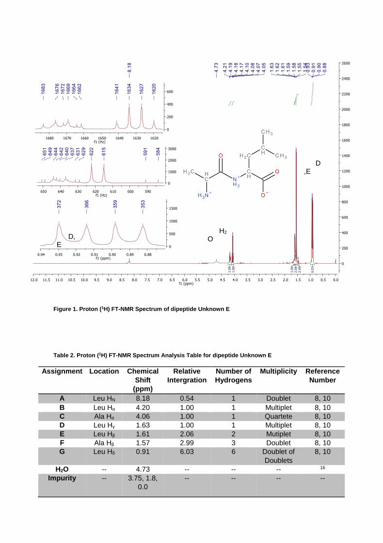
Figure 1. Proton (1H) FT-NMR Spectrum of dipeptide Unknown E
Table 2. Proton (1H) FT-NMR Spectrum Analysis Table for dipeptide Unknown E
Assignment Location Chemical
Shift
(ppm)
Relative
Intergration
Number of
Hydrogens
Multiplicity Reference
Number
A Leu HN 8.18 0.54 1 Doublet 8, 10
B Leu Hα 4.20 1.00 1 Multiplet 8, 10
C Ala Hα 4.06 1.00 1 Quartete 8, 10
D Leu Hγ 1.63 1.00 1 Multiplet 8, 10
E Leu Hβ 1.61 2.06 2 Mutiplet 8, 10
F Ala Hβ 1.57 2.99 3 Doublet 8, 10
G Leu Hδ 0.91 6.03 6 Doublet of
Doublets
8, 10
H2O -- 4.73 -- -- -- 16
Impurity -- 3.75, 1.8,
0.0
-- -- -- --
A
H2
O
B C
D,E
F
G
A
B
C
D
G
G E
F
B C
D, E
F
G
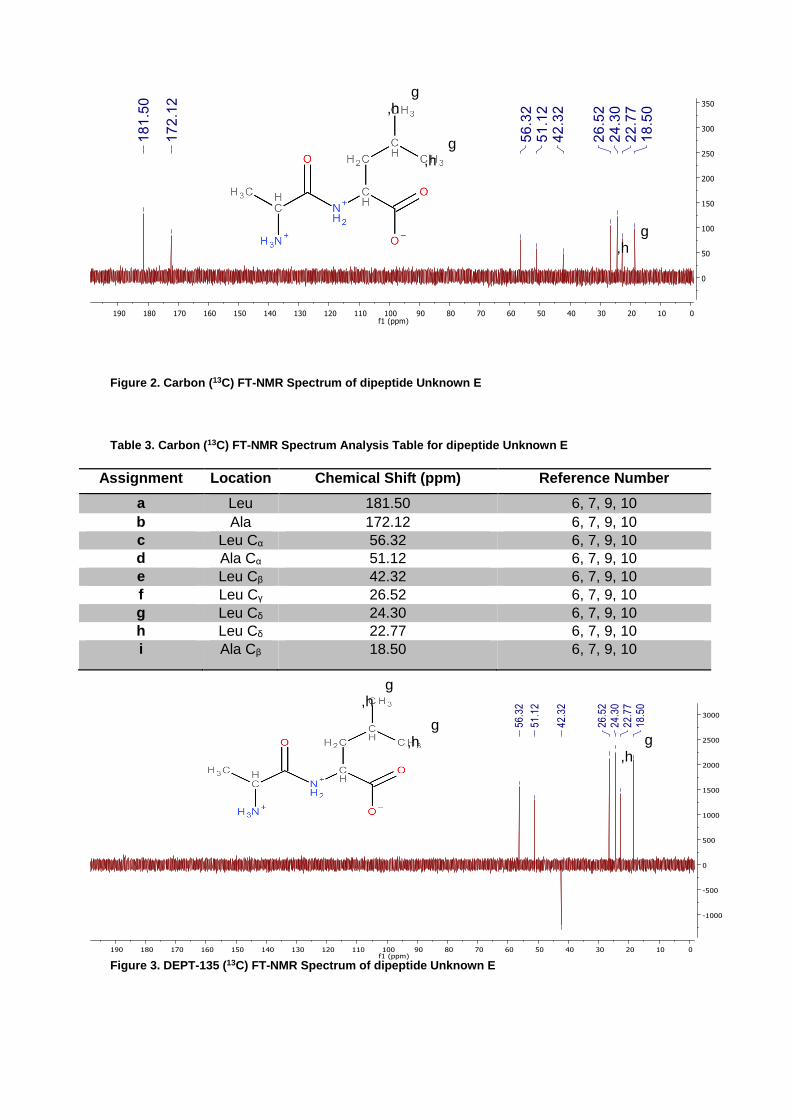
Figure 2. Carbon (13C) FT-NMR Spectrum of dipeptide Unknown E
Table 3. Carbon (13C) FT-NMR Spectrum Analysis Table for dipeptide Unknown E
Assignment Location Chemical Shift (ppm) Reference Number
a Leu 181.50 6, 7, 9, 10
b Ala 172.12 6, 7, 9, 10
c Leu Cα 56.32 6, 7, 9, 10
d Ala Cα 51.12 6, 7, 9, 10
e Leu Cβ 42.32 6, 7, 9, 10
f Leu Cγ 26.52 6, 7, 9, 10
g Leu Cδ 24.30 6, 7, 9, 10
h Leu Cδ 22.77 6, 7, 9, 10
i Ala Cβ 18.50 6, 7, 9, 10
Figure 3. DEPT-135 (13C) FT-NMR Spectrum of dipeptide Unknown E
a
b
c
d
e
i
f
g,h
g,h
a b
c
d
e
i
f
g,h
g,h
a
b
c d e f
g,h
i
c d
e
f
g,h
i
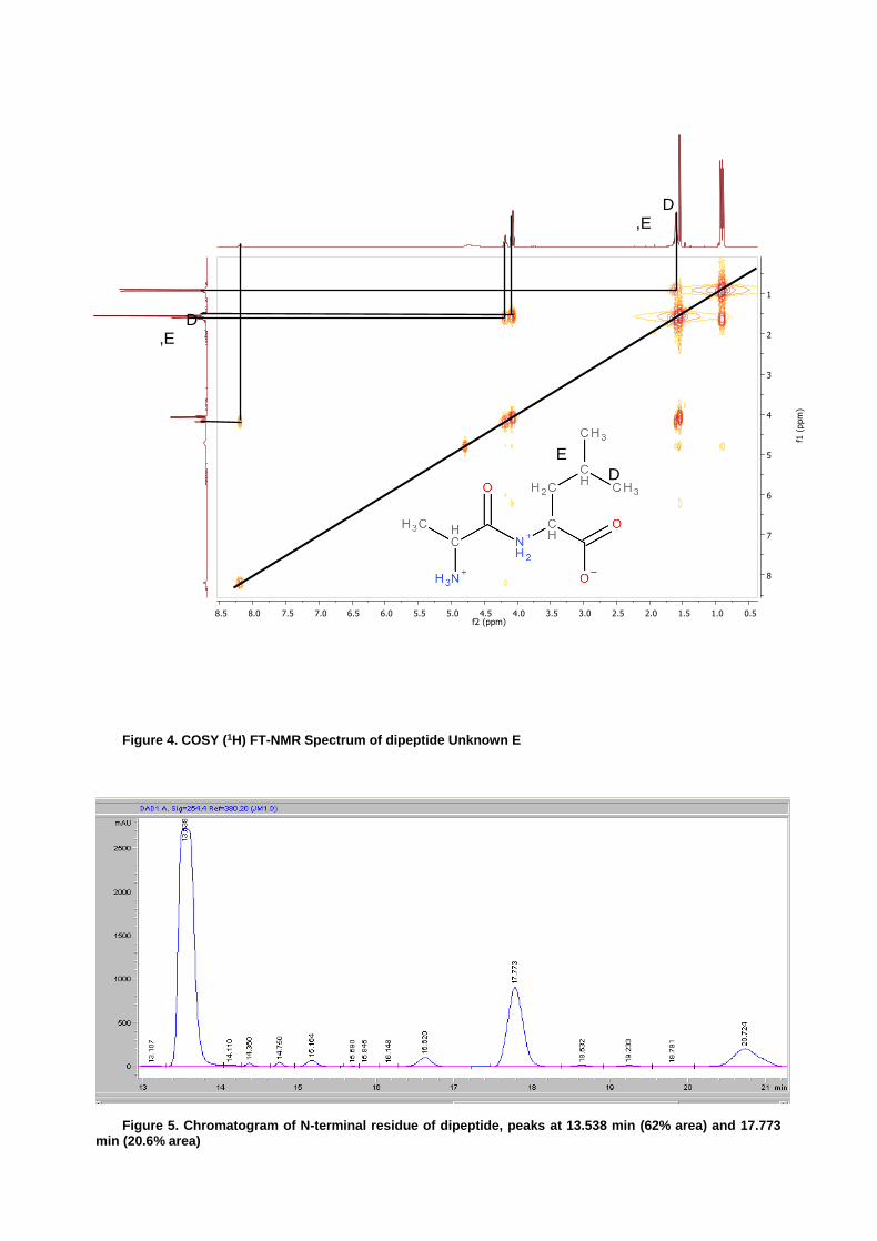
Figure 4. COSY (1H) FT-NMR Spectrum of dipeptide Unknown E
Figure 5. Chromatogram of N-terminal residue of dipeptide, peaks at 13.538 min (62% area) and 17.773 min (20.6% area)
A B C
D,E
F
G
B
C
D,E
F
G
A
B
C D
F
G
G E
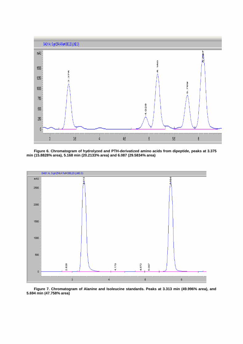
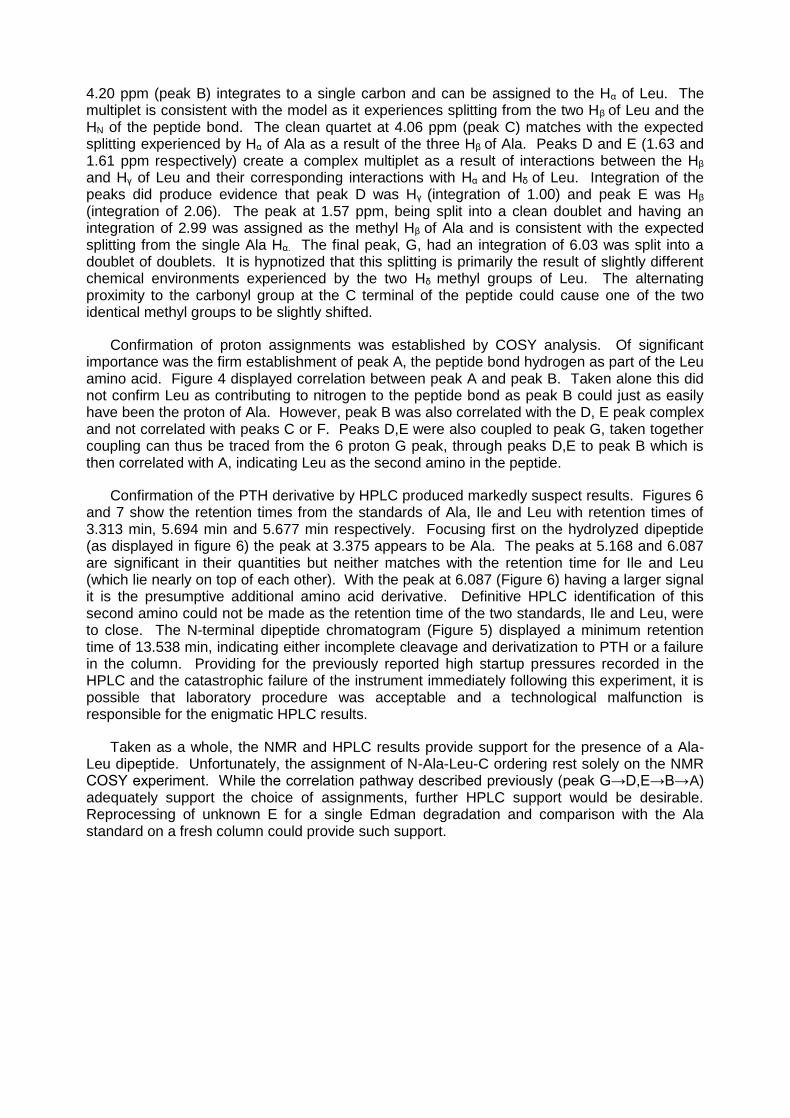
Figure 6. Chromatogram of hydrolyzed and PTH-derivatized amino acids from dipeptide, peaks at 3.375 min (15.8828% area), 5.168 min (20.2133% area) and 6.087 (29.5834% area)
Figure 7. Chromatogram of Alanine and Isoleucine standards. Peaks at 3.313 min (49.996% area), and 5.694 min (47.758% area)
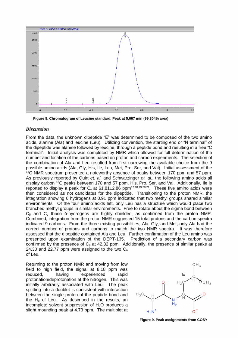
Figure 8. Chromatogram of Leucine standard. Peak at 5.667 min (99.304% area)
Discussion
From the data, the unknown dipeptide “E” was determined to be composed of the two amino acids, alanine (Ala) and leucine (Leu). Utilizing convention, the starting end or “N terminal” of the dipeptide was alanine followed by leucine, through a peptide bond and resulting in a free “C terminal”. Initial analysis was completed by NMR which allowed for full determination of the number and location of the carbons based on proton and carbon experiments. The selection of the combination of Ala and Leu resulted from first narrowing the available choice from the 9 possible amino acids (Ala, Gly, His, Ile, Leu, Met, Pro, Ser, and Val). Initial assessment of the 13C NMR spectrum presented a noteworthy absence of peaks between 170 ppm and 57 ppm. As previously reported by Quirt et. al. and Schwarzinger et. al., the following amino acids all display carbon 13C peaks between 170 and 57 ppm, His, Pro, Ser, and Val. Additionally, Ile is reported to display a peak for Cα at 61.81±2.86 ppm17,18,19,20,21. These five amino acids were then considered as not candidates for the dipeptide. Transitioning to the proton NMR, the integration showing 6 hydrogens at 0.91 ppm indicated that two methyl groups shared similar environments. Of the four amino acids left, only Leu has a structure which would place two branched methyl groups in similar environments. Free to rotate about the sigma bond between Cβ and Cγ these δ-hydrogens are highly shielded, as confirmed from the proton NMR. Combined, integration from the proton NMR suggested 15 total protons and the carbon spectra indicated 9 carbons. From the three existing possibilities, Ala, Gly, and Met, only Ala had the correct number of protons and carbons to match the two NMR spectra. It was therefore assessed that the dipeptide contained Ala and Leu. Further confirmation of the Leu amino was presented upon examination of the DEPT-135. Prediction of a secondary carbon was confirmed by the presence of Cβ at 42.32 ppm. Additionally, the presence of similar peaks at 24.30 and 22.77 ppm were assigned to the two Cδ of Leu.
Returning to the proton NMR and moving from low field to high field, the signal at 8.18 ppm was reduced, having experienced rapid protonation/deprotonation at the nitrogen. This was initially arbitrarily associated with Leu. The peak splitting into a doublet is consistent with interaction between the single proton of the peptide bond and the Hα of Leu. As described in the results, an incomplete solvent suppression of H2O produces a slight mounding peak at 4.73 ppm. The multiplet at
A
B
C
D
F
G
G E
Figure 9. Peak assignments from COSY
4.20 ppm (peak B) integrates to a single carbon and can be assigned to the Hα of Leu. The multiplet is consistent with the model as it experiences splitting from the two Hβ of Leu and the HN of the peptide bond. The clean quartet at 4.06 ppm (peak C) matches with the expected splitting experienced by Hα of Ala as a result of the three Hβ of Ala. Peaks D and E (1.63 and 1.61 ppm respectively) create a complex multiplet as a result of interactions between the Hβ and Hγ of Leu and their corresponding interactions with Hα and Hδ of Leu. Integration of the peaks did produce evidence that peak D was Hγ (integration of 1.00) and peak E was Hβ (integration of 2.06). The peak at 1.57 ppm, being split into a clean doublet and having an integration of 2.99 was assigned as the methyl Hβ of Ala and is consistent with the expected splitting from the single Ala Hα. The final peak, G, had an integration of 6.03 was split into a doublet of doublets. It is hypnotized that this splitting is primarily the result of slightly different chemical environments experienced by the two Hδ methyl groups of Leu. The alternating proximity to the carbonyl group at the C terminal of the peptide could cause one of the two identical methyl groups to be slightly shifted.
Confirmation of proton assignments was established by COSY analysis. Of significant importance was the firm establishment of peak A, the peptide bond hydrogen as part of the Leu amino acid. Figure 4 displayed correlation between peak A and peak B. Taken alone this did not confirm Leu as contributing to nitrogen to the peptide bond as peak B could just as easily have been the proton of Ala. However, peak B was also correlated with the D, E peak complex and not correlated with peaks C or F. Peaks D,E were also coupled to peak G, taken together coupling can thus be traced from the 6 proton G peak, through peaks D,E to peak B which is then correlated with A, indicating Leu as the second amino in the peptide.
Confirmation of the PTH derivative by HPLC produced markedly suspect results. Figures 6 and 7 show the retention times from the standards of Ala, Ile and Leu with retention times of 3.313 min, 5.694 min and 5.677 min respectively. Focusing first on the hydrolyzed dipeptide (as displayed in figure 6) the peak at 3.375 appears to be Ala. The peaks at 5.168 and 6.087 are significant in their quantities but neither matches with the retention time for Ile and Leu (which lie nearly on top of each other). With the peak at 6.087 (Figure 6) having a larger signal it is the presumptive additional amino acid derivative. Definitive HPLC identification of this second amino could not be made as the retention time of the two standards, Ile and Leu, were to close. The N-terminal dipeptide chromatogram (Figure 5) displayed a minimum retention time of 13.538 min, indicating either incomplete cleavage and derivatization to PTH or a failure in the column. Providing for the previously reported high startup pressures recorded in the HPLC and the catastrophic failure of the instrument immediately following this experiment, it is possible that laboratory procedure was acceptable and a technological malfunction is responsible for the enigmatic HPLC results.
Taken as a whole, the NMR and HPLC results provide support for the presence of a Ala-Leu dipeptide. Unfortunately, the assignment of N-Ala-Leu-C ordering rest solely on the NMR COSY experiment. While the correlation pathway described previously (peak G→D,E→B→A) adequately support the choice of assignments, further HPLC support would be desirable. Reprocessing of unknown E for a single Edman degradation and comparison with the Ala standard on a fresh column could provide such support.
References
Rausch, C.; Weber, T.; Kohlbacher, O.; Wohlleben, W.; Huson, D. Specificity prediction of
adenylation domains in nonribosomal peptide synthetases (NRPS) using transductive support
vector machines (TSVMs). Nucleic Acids Res.2005, 33, 5799-5808.
Kohen, R.; Yamamoto, Y.; Ames, B. N. Antioxidant activity of carnosine, homocarnosine, and anserine present in muscle and brain. Proc. Natl. Acad. Sci. USA 1988, 85, 3175-3179. Nakajima, T.; Wolfgram, F.; Clark, W. G. THE ISOLACTION OF HOMOANSERINE FROM BOVINE BRAIN. J. Neurochem. 1967, 14, 1107-1112.
Edmand, P.; Hogfeldt, E.; Sillen, L. G.; Kinell, P. Method for determination of the amino acid
sequence of peptides. Acta Chem. Scand. 1950, 4, 283-293.
Pisano, J. J.; Bronzert, T. J. Advances in the gas chromatographic analysis of amino acid pheny-
and methythiohydantions. Anal. Biochem. 1972, 45, 43-59.
Gottlieb, H. E.; Kotlyar, V.; Nudelman, A. NMR Chemical shifts of Common Laboratory
Solvents as trace impurities. J. Org. Chem. 1997, 62, 7512-7515.
Quirt, A. R.; Lyerla, J. R., Peat, I. R.; Cohen, J. S., Reynolds, W. F., Freedman, M. H. Carbon-13 Nuclear Magnetic Resonance Titration Shifts in Amino Acids. J. AM. Chem. Soc. 1974, 96, 570-574.
Schwarzinger, S.; Kroon, G. J. A.; Foss, T. R.; Wright, P. E.; Dyson, H. J. Random coil
chemical shifts in acidic 8M urea: implementation of random coil shift data in NMRView. J.
Biomol. NMR, 2000, 18, 43-48.
Bundi, A. and Wuthrich, K. 1H-NMR parameters of the Common Amino Acid Residues Measured in Aqueous Solutions of the Linear Tetrapeptides H-Gly-Gly-X-L-Ala-OH. Biopolymers, 1979, 18, 285-297.
Richarz, R. and Wuthrich, K. Carbon-13 NMR chemical Shifts of the Common Amino Acid Residues Measured in Aqueous Solutions of the Linear Tetrapeptides H-Gly-Gly-X-L-Ala-OH. Biopolymers, 1978, 17, 2133-2141.
Wuthrich, K. NMR in Biological Research: Pepdtides and Proteins. North Holland, Amsterdam
, 1976.
Mark Weir February 20, 2013
Simultaneous Determination of Caffeine and Benzoic Acid in Mountain Dew by
Ultraviolet Spectroscopy
Introduction
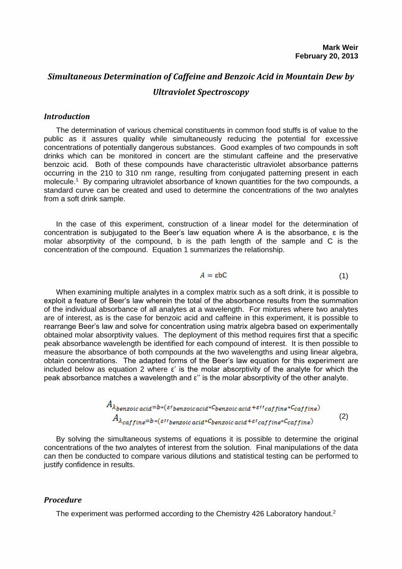
The determination of various chemical constituents in common food stuffs is of value to the public as it assures quality while simultaneously reducing the potential for excessive concentrations of potentially dangerous substances. Good examples of two compounds in soft drinks which can be monitored in concert are the stimulant caffeine and the preservative benzoic acid. Both of these compounds have characteristic ultraviolet absorbance patterns occurring in the 210 to 310 nm range, resulting from conjugated patterning present in each molecule.1 By comparing ultraviolet absorbance of known quantities for the two compounds, a standard curve can be created and used to determine the concentrations of the two analytes from a soft drink sample.
In the case of this experiment, construction of a linear model for the determination of
concentration is subjugated to the Beer’s law equation where A is the absorbance, ɛ is the molar absorptivity of the compound, b is the path length of the sample and C is the concentration of the compound. Equation 1 summarizes the relationship.
When examining multiple analytes in a complex matrix such as a soft drink, it is possible to
exploit a feature of Beer’s law wherein the total of the absorbance results from the summation of the individual absorbance of all analytes at a wavelength. For mixtures where two analytes are of interest, as is the case for benzoic acid and caffeine in this experiment, it is possible to rearrange Beer’s law and solve for concentration using matrix algebra based on experimentally obtained molar absorptivity values. The deployment of this method requires first that a specific peak absorbance wavelength be identified for each compound of interest. It is then possible to measure the absorbance of both compounds at the two wavelengths and using linear algebra, obtain concentrations. The adapted forms of the Beer’s law equation for this experiment are included below as equation 2 where ε’ is the molar absorptivity of the analyte for which the peak absorbance matches a wavelength and ε’’ is the molar absorptivity of the other analyte.
By solving the simultaneous systems of equations it is possible to determine the original concentrations of the two analytes of interest from the solution. Final manipulations of the data can then be conducted to compare various dilutions and statistical testing can be performed to justify confidence in results.
Procedure
The experiment was performed according to the Chemistry 426 Laboratory handout.2
(1)
(2)
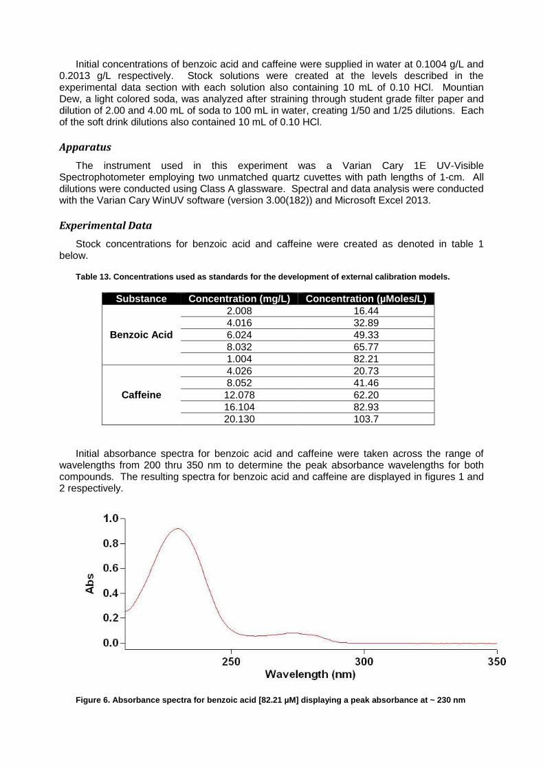
Initial concentrations of benzoic acid and caffeine were supplied in water at 0.1004 g/L and 0.2013 g/L respectively. Stock solutions were created at the levels described in the experimental data section with each solution also containing 10 mL of 0.10 HCl. Mountian Dew, a light colored soda, was analyzed after straining through student grade filter paper and dilution of 2.00 and 4.00 mL of soda to 100 mL in water, creating 1/50 and 1/25 dilutions. Each of the soft drink dilutions also contained 10 mL of 0.10 HCl.
Apparatus
The instrument used in this experiment was a Varian Cary 1E UV-Visible Spectrophotometer employing two unmatched quartz cuvettes with path lengths of 1-cm. All dilutions were conducted using Class A glassware. Spectral and data analysis were conducted with the Varian Cary WinUV software (version 3.00(182)) and Microsoft Excel 2013.
Experimental Data
Stock concentrations for benzoic acid and caffeine were created as denoted in table 1 below.
Table 13. Concentrations used as standards for the development of external calibration models.
Substance Concentration (mg/L) Concentration (µMoles/L)
Benzoic Acid
2.008 16.44
4.016 32.89
6.024 49.33
8.032 65.77
1.004 82.21
Caffeine
4.026 20.73
8.052 41.46
12.078 62.20
16.104 82.93
20.130 103.7
Initial absorbance spectra for benzoic acid and caffeine were taken across the range of wavelengths from 200 thru 350 nm to determine the peak absorbance wavelengths for both compounds. The resulting spectra for benzoic acid and caffeine are displayed in figures 1 and 2 respectively.
Figure 6. Absorbance spectra for benzoic acid [82.21 µM] displaying a peak absorbance at ~ 230 nm
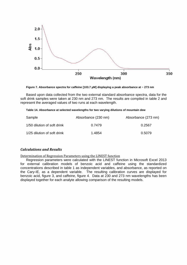
Figure 7. Absorbance spectra for caffeine [103.7 µM] displaying a peak absorbance at ~ 273 nm
Based upon data collected from the two external standard absorbance spectra, data for the soft drink samples were taken at 230 nm and 273 nm. The results are compiled in table 2 and represent the averaged values of two runs at each wavelength.
Table 14. Absorbance at selected wavelengths for two varying dilutions of mountain dew
Sample Absorbance (230 nm) Absorbance (273 nm)
1/50 dilution of soft drink 0.7479 0.2567
1/25 dilution of soft drink 1.4854 0.5079
Calculations and Results
Determination of Regression Parameters using the LINEST function Regression parameters were calculated with the LINEST function in Microsoft Excel 2013
for external calibration models of benzoic acid and caffeine using the standardized concentrations described in table 1 as independent variables, and absorbance, as reported on the Cary-IE, as a dependent variable. The resulting calibration curves are displayed for benzoic acid, figure 3, and caffeine, figure 4. Data at 230 and 273 nm wavelengths has been displayed together for each analyte allowing comparison of the resulting models.
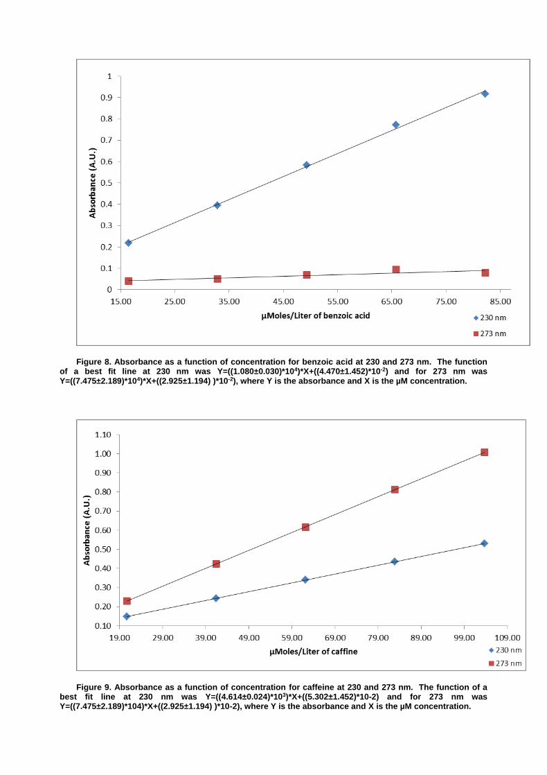
Figure 8. Absorbance as a function of concentration for benzoic acid at 230 and 273 nm. The function of a best fit line at 230 nm was Y=((1.080±0.030)*104)*X+((4.470±1.452)*10-2) and for 273 nm was Y=((7.475±2.189)*104)*X+((2.925±1.194) )*10-2), where Y is the absorbance and X is the µM concentration.
Figure 9. Absorbance as a function of concentration for caffeine at 230 and 273 nm. The function of a best fit line at 230 nm was Y=((4.614±0.024)*103)*X+((5.302±1.452)*10-2) and for 273 nm was Y=((7.475±2.189)*104)*X+((2.925±1.194) )*10-2), where Y is the absorbance and X is the µM concentration.

LINEST results for each model are summarized in table 3 where A.U is absorbance units as reported by the Cary IE and µM is the micro molarity of the sample.
Table 15. Linear regression parameters for each model as calculated with the LINEST function in Microsoft Excel
Regression Parameter
Benzoic Acid (230 nm)
Benzoic Acid (273 nm)
Caffeine (230 nm)
Caffeine (273 nm)
Slope (A.U. * µM-1)
(1.080±0.027)*10-2 (7.465±2.189)*10-4 (4.614±0.024)*10-3 (9.384±0.014)*10-3
y-intercept (A.U.)
(4.473±1.449)*10-2 (2.925±1.194)*10-2 (5.302±0.165)*10-2 (3.420±0.100)*10-2
Coefficient of Determination (R2)
0.9982 0.7950 0.9999 1.000
Standard Error of Estimate (SEE)
0.01382 0.01138 0.001570 0.0009504
F-Statistic 1651 11.63 37110 419000
In addition to the LINEST calculated values organized in table 2, additional figures of merit including percent relative standard deviation of the slope (%RSD), the confidence interval about the y-intercept, and the detection limit, were calculated for each model. Respective sample calculation for each can be found in equations 2, 3, and 4 below employing the data from benzoic acid as measured at 230 nm. For these calculations, m is the slope of the linear regression model, b is the y-intercept and σ is the standard deviation about a figure. For the calculation of the confidence interval about b, the 95% confidence level is evaluated using calculations where the z-value is 1.96. The resulting figures of merit are presented in table 4.
Table 16.Figures of merit for each of the external standard models
Figure of Merit Benzoic Acid (230 nm)
Benzoic Acid (273 nm)
Caffeine (230 nm)
Caffeine (273 nm)
%RSD 2.5% 29.3% 0.5% 0.2%
Confidence about the y-intercept
(A.U.)
0.04473±0.02841 0.02925±0.02339 0.05302±0.00323 0.03420±0.00195
Detection Limit (µmol L-1)
4.026 47.97 1.071 0.3187

From the figures of merit in table 4 there exists a y-intercept bias in each of the models. No model contained the value of zero for the y-intercept at the 95% confidence interval. Additionally, because of the lower %RSD values and detection limits, 230 nm was selected for benzoic acid and 273 nm was selected for caffeine.
Based upon the multiple analyte linear algebra formulas presented in the introduction, a set of simultaneous equations were solved using Microsoft Excel 2013. Owing to the 1.00 cm path length of the quartz cuvette used, the molar absorptivity for each analyte is the slope of the regression line reported in table 3. These values were assembled in an array and the inverse molar absorptivity matrix was established with the MINVERSE command in Microsoft Excel. The resulting values are compiled in table 5.
Table 17.Inverse molar absorptivity values as calculated from a matrix with Microsoft Excel.
Wavelength Benzoic Acid (ε-1) Caffeine (ε-1)
230 95.86 -47.13
273 -7.626 110.3
The values presented in table 5 were then processed with the absorbance for each of the soft drink samples as presented in table 2 using the MMULT function in Microsoft Excel. The resulting concentrations, as developed from the solving of a simultaneous system of equations, are summarized in table 6. The solution to the equations returned a micro molar volume which was converted to mg per L by equation 6.
Table 18. Diluted soft drink concentrations as determined by solving of simultaneous systems of equations.
Sample Benzoic Acid (µM)
Caffeine (µM)
Benzoic Acid (mg/L)
Caffeine (mg/L)
1/50 dilution of soft drink
59.59 22.61 7.278±0.001 4.389±0.003
1/25 dilution of soft drink
118.5 44.64 14.46±0.01 8.676±0.009
By using the concentration equation, C1V1=C2V2, and the values obtained in table 6, the original concentration of each analyte can be determined. A sample calculation for the dilution is displayed for benzoic acid in the 1/50 dilution as equation 7 along with the propagation of error in equation 8. Values for the original concentrations for both analytes in both samples is summarized in table 7.
Table 19. Calculated original concentrations in soft drink samples
Sample Benzoic Acid (mg/L) Caffeine (mg/L)
1/50 dilution of soft drink 363.9±1.1 219.5±0.7
1/25 dilution of soft drink 361.5±1.0 216.9±0.6
The presence of two values for concentrations, resulting from various dilutions of the original soft drink sample, allows for a statistical F test to be performed on the standard deviations of the two samples. The F test for benzoic acid returned a value of 1.21 vs a critical value of 39 (0.05, 2, 2) at the 95% confidence interval. For caffeine the test returned a value of 1.36 vs a critical value of 39 (0.05, 2, 2). In neither case did the test suggest significant variance at the 95% confidence level, a sample of the benzoic acid test calculation can be found in equation 9.
The absence of significant differences in the deviations allows for the performance of a two tailed T-test to determine if the concentrations calculated from the two dilutions are similar at the 95% confidence interval. A sample calculation for benzoic acid can be found in equation 10. The resulting experimental T values of 2.28 for benzoic acid and 3.91 for caffeine are below the critical T value of 4.303 (0.05, 2), thus the values can be consider similar at the 95% confidence interval.
The soft drink manufacture indicates the amount of caffeine on the side of their can. The reported value is 218.2 mg/L. Based on calculation in equation 11, the percent relative error in our determination is 43.46%.
Discussion
The concentrations for benzoic acid and caffeine in a lightly colored soft drink sample have been determined by the absorbance at two wavelength, 230 nm and 273 nm. Solving for a simultaneous systems of equations as resulted in an average benzoic acid concentration of 362.7±1.1 mg/L and an average caffeine concentration of 218.2±0.7 mg/L. The experimental results from the two dilutions match closely with each other, satisfying statistical test at the 95% confidence interval. The percent relative error of the caffeine concentration, indicating a major deviation from the manufactures stated caffeine concentration of 152.2 mg/L, is troublesome and may indicate determinate errors in the underlying method of calculation or detection. This is supported by a y-intercept bias in all four of the models summarized in table 4. Additionally, while the caffeine models have low percent relative standard deviations at both wavelengths, the benzoic acid model has a high relative standard deviation at 273 nm and a notable %RSD at 230 nm. Since reading at both wavelengths are used in the final calculation of the concentration, an inaccurate model may have skewed final concentration results. Additional testing and identification of the benzoic acid and caffeine absorbance spectra would provide confirmation that 273 and 230 nm are the best wavelengths for concentrations determination with these two analytes.
One potential area of concern in this method when determining the concentrations of
benzoic acid and caffeine is the presupposition that no other analytes present as components of the soft drink matrix absorb at 230 or 273 nm. If there was another component of the soft drink which did absorb, the linear algebra calculations would be off and the values would be skewed, as could have occurred in our results. By utilizing another method, namely high performance liquid chromatography, the analytes can be separated from each other and additional matrix components. This would allow for more precise analysis of the individual components and, by employing an internal standard, increasingly accurate direct determination of the analytes concentrations.
References
2. Sharma, B. K. (1981). Spectroscopy. Krishna Prakashasn Media.
3. Chemistry 426: Instrumental Analysis Laboratory Manual, Department of Chemistry,
Southern Oregon University: Ashland, OR, 2014.
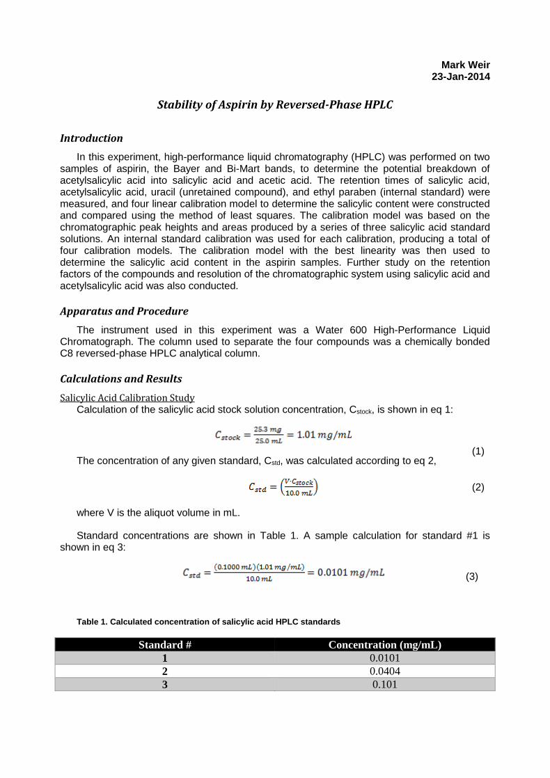
Mark Weir 23-Jan-2014
Stability of Aspirin by Reversed-Phase HPLC
Introduction
In this experiment, high-performance liquid chromatography (HPLC) was performed on two samples of aspirin, the Bayer and Bi-Mart bands, to determine the potential breakdown of acetylsalicylic acid into salicylic acid and acetic acid. The retention times of salicylic acid, acetylsalicylic acid, uracil (unretained compound), and ethyl paraben (internal standard) were measured, and four linear calibration model to determine the salicylic content were constructed and compared using the method of least squares. The calibration model was based on the chromatographic peak heights and areas produced by a series of three salicylic acid standard solutions. An internal standard calibration was used for each calibration, producing a total of four calibration models. The calibration model with the best linearity was then used to determine the salicylic acid content in the aspirin samples. Further study on the retention factors of the compounds and resolution of the chromatographic system using salicylic acid and acetylsalicylic acid was also conducted.
Apparatus and Procedure
The instrument used in this experiment was a Water 600 High-Performance Liquid Chromatograph. The column used to separate the four compounds was a chemically bonded C8 reversed-phase HPLC analytical column.
Calculations and Results
Salicylic Acid Calibration Study Calculation of the salicylic acid stock solution concentration, Cstock, is shown in eq 1:
The concentration of any given standard, Cstd, was calculated according to eq 2,
where V is the aliquot volume in mL.
Standard concentrations are shown in Table 1. A sample calculation for standard #1 is shown in eq 3:
Table 1. Calculated concentration of salicylic acid HPLC standards
Standard # Concentration (mg/mL)
1 0.0101
2 0.0404
3 0.101
(1)
(3)
(2)
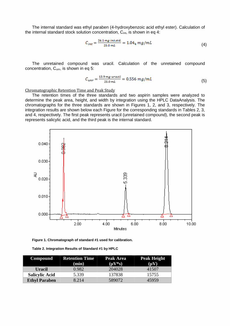
The internal standard was ethyl paraben (4-hydroxybenzoic acid ethyl ester). Calculation of the internal standard stock solution concentration, Cint, is shown in eq 4:
The unretained compound was uracil. Calculation of the unretained compound concentration, Cunr, is shown in eq 5:
Chromatographic Retention Time and Peak Study The retention times of the three standards and two aspirin samples were analyzed to
determine the peak area, height, and width by integration using the HPLC DataAnalysis. The chromatographs for the three standards are shown in Figures 1, 2, and 3, respectively. The integration results are shown below each Figure for the corresponding standards in Tables 2, 3, and 4, respectively. The first peak represents uracil (unretained compound), the second peak is represents salicylic acid, and the third peak is the internal standard.
Figure 1. Chromatograph of standard #1 used for calibration.
Table 2. Integration Results of Standard #1 by HPLC
Compound Retention Time
(min)
Peak Area
(µV*s)
Peak Height
(µV)
Uracil 0.982 204028 41507
Salicylic Acid 5.339 137838 15755
Ethyl Paraben 8.214 589072 45959
(4)
(5)

Figure 2. Chromatograph of standard #2 used for calibration.
Table 3. Integration Results of Standard #2 by HPLC
Compound Retention Time
(min)
Peak Area
(µV*s)
Peak Height
(µV)
Uracil 0.957 181838 36736
Salicylic Acid 5.276 1165208 133416
Ethyl Paraben 8.190 782935 60747
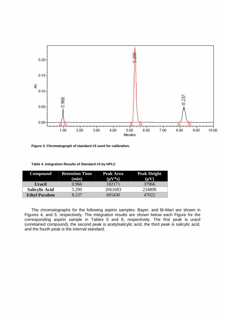
Figure 3. Chromatograph of standard #3 used for calibration.
Table 4. Integration Results of Standard #3 by HPLC
Compound Retention Time
(min)
Peak Area
(µV*s)
Peak Height
(µV)
Uracil 0.966 182171 37966
Salicylic Acid 5.290 2061683 234898
Ethyl Paraben 8.237 605430 47022
The chromatographs for the following aspirin samples: Bayer, and Bi-Mart are shown in Figures 4, and 5, respectively. The integration results are shown below each Figure for the corresponding aspirin sample in Tables 5 and 6, respectively. The first peak is uracil (unretained compound), the second peak is acetylsalicylic acid, the third peak is salicylic acid, and the fourth peak is the internal standard.
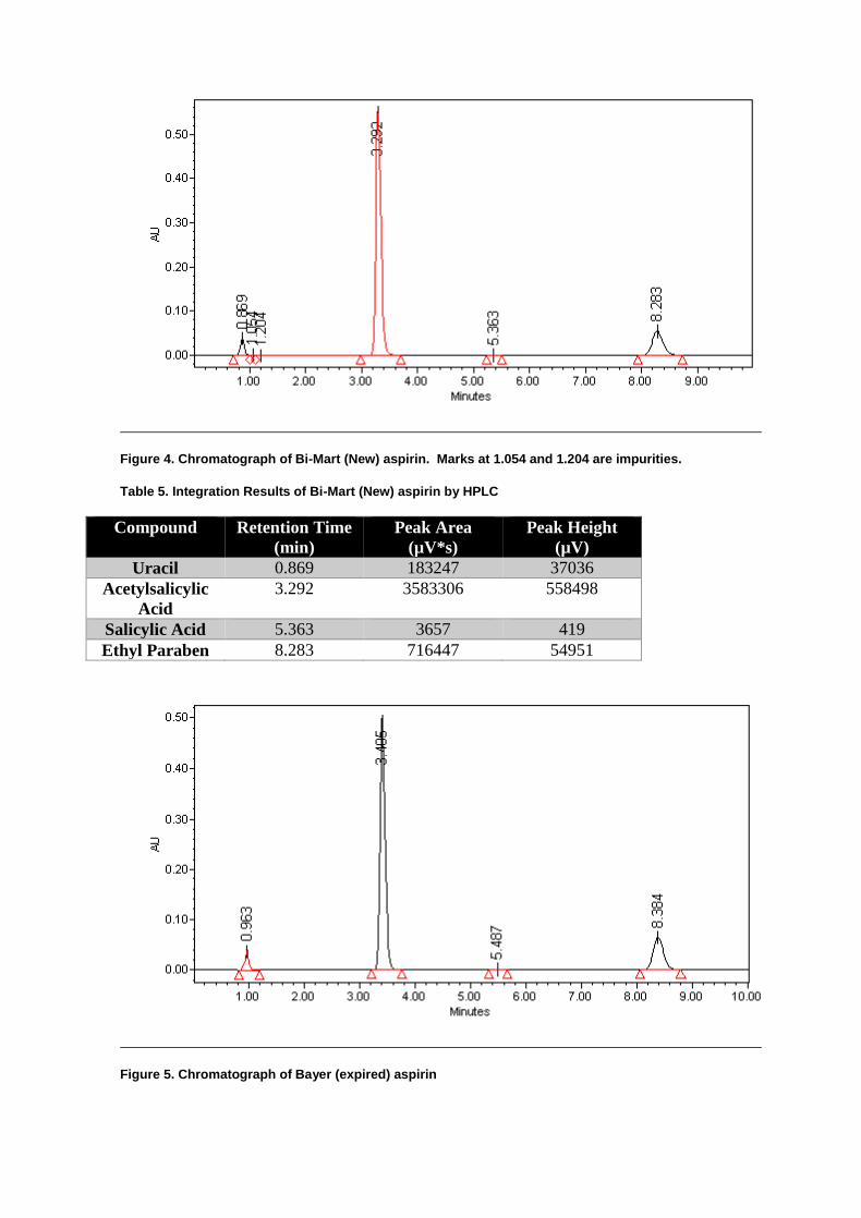
Figure 4. Chromatograph of Bi-Mart (New) aspirin. Marks at 1.054 and 1.204 are impurities.
Table 5. Integration Results of Bi-Mart (New) aspirin by HPLC
Compound Retention Time
(min)
Peak Area
(µV*s)
Peak Height
(µV)
Uracil 0.869 183247 37036
Acetylsalicylic
Acid
3.292 3583306 558498
Salicylic Acid 5.363 3657 419
Ethyl Paraben 8.283 716447 54951
Figure 5. Chromatograph of Bayer (expired) aspirin

Table 6. Integration Results of Bayer (expired) aspirin by HPLC
Compound Retention Time
(min)
Peak Area
(µV*s)
Peak Height
(µV)
Uracil 0.963 196510 38036
Acetylsalicylic
Acid
3.405 3222725 499867
Salicylic Acid 5.487 14388 1552
Ethyl Paraben 8.384 838845 64701
Determination of salicylic acid in aspirin requires the peak areas and heights for the salicylic acid standards along with the internal standard. The ratio of the salicylic acid peak with the internal standard peak was determined and the results for peak areas and peak heights are shown in Tables 7 and 8, respectively.
Table 7. Quantitative results of salicylic acid determination using HPLC peak areas
Concentration of
Salicylic Acid
(mg/mL)
Salicylic Acid
Peak Area
(µV*s)
Ethyl Paraben
Peak Area
(µV*s)
Ratio of Salicylic
Acid/Ethyl Paraben
0.0101 137838 589072 0.233992
0.0404 1165208 782935 1.48826
0.101 2061683 605430 3.40532
Table 8. Quantitative results of salicylic acid determination using HPLC peak heights
Concentration of
Salicylic Acid
(mg/mL)
Salicylic Acid
Peak Height
(µV)
Ethyl Paraben
Peak Height
(µV)
Ratio of Salicylic
Acid/Ethyl Paraben
Peak Height
0.0101 15755 45959 0.34281
0.0404 133416 60747 2.19626
0.101 234898 47022 4.9955
Calculation of Calibration Model A least-squares calculation was used to compute the slope, intercept, and their standard
deviations using a linear calibration model for the data in Tables 7 and 8 for both external and internal calibration. The regression function in the Microsoft Excel LINEST Data Analysis Toolpak was used for this calculation. The results for both peak areas and heights using external calibration are shown as equations 5 and 6, respectively. The results for both peak areas and heights using internal calibration are shown as equations 7 and 8, respectively.
(6)
(5)
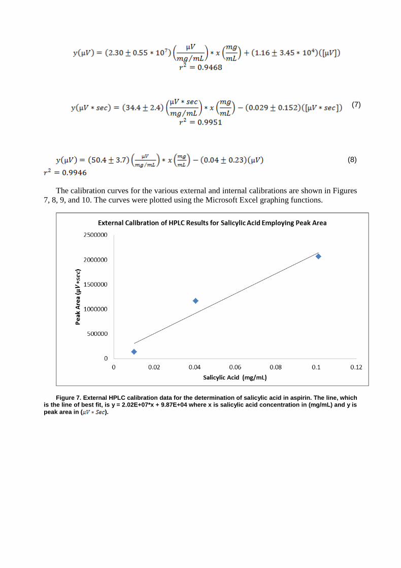
The calibration curves for the various external and internal calibrations are shown in Figures
7, 8, 9, and 10. The curves were plotted using the Microsoft Excel graphing functions.
Figure 7. External HPLC calibration data for the determination of salicylic acid in aspirin. The line, which is the line of best fit, is y = 2.02E+07*x + 9.87E+04 where x is salicylic acid concentration in (mg/mL) and y is
peak area in ( ).
(7)
(8)
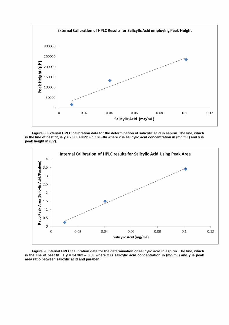
Figure 8. External HPLC calibration data for the determination of salicylic acid in aspirin. The line, which is the line of best fit, is y = 2.30E+06*x + 1.16E+04 where x is salicylic acid concentration in (mg/mL) and y is peak height in (µV).
Figure 9. Internal HPLC calibration data for the determination of salicylic acid in aspirin. The line, which is the line of best fit, is y = 34.36x – 0.03 where x is salicylic acid concentration in (mg/mL) and y is peak area ratio between salicylic acid and paraben.
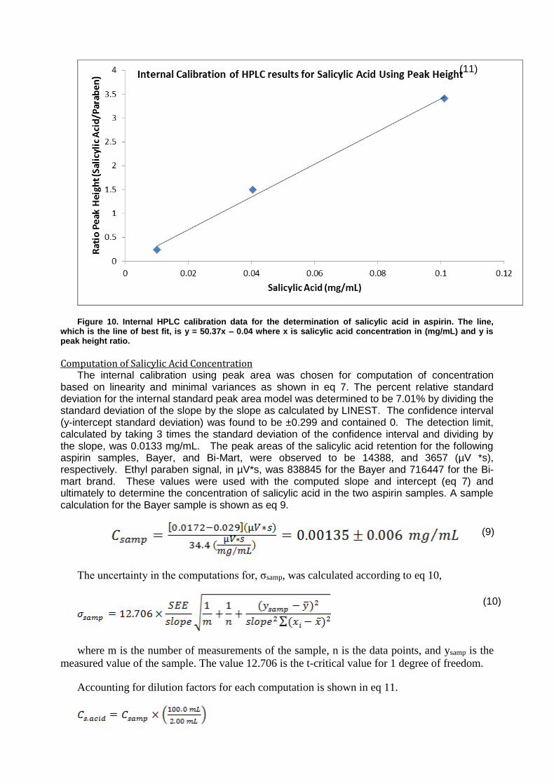
Figure 10. Internal HPLC calibration data for the determination of salicylic acid in aspirin. The line, which is the line of best fit, is y = 50.37x – 0.04 where x is salicylic acid concentration in (mg/mL) and y is peak height ratio.
Computation of Salicylic Acid Concentration The internal calibration using peak area was chosen for computation of concentration
based on linearity and minimal variances as shown in eq 7. The percent relative standard deviation for the internal standard peak area model was determined to be 7.01% by dividing the standard deviation of the slope by the slope as calculated by LINEST. The confidence interval (y-intercept standard deviation) was found to be ±0.299 and contained 0. The detection limit, calculated by taking 3 times the standard deviation of the confidence interval and dividing by the slope, was 0.0133 mg/mL. The peak areas of the salicylic acid retention for the following aspirin samples, Bayer, and Bi-Mart, were observed to be 14388, and 3657 (µV *s), respectively. Ethyl paraben signal, in µV*s, was 838845 for the Bayer and 716447 for the Bi-mart brand. These values were used with the computed slope and intercept (eq 7) and ultimately to determine the concentration of salicylic acid in the two aspirin samples. A sample calculation for the Bayer sample is shown as eq 9.
The uncertainty in the computations for, σsamp, was calculated according to eq 10,
where m is the number of measurements of the sample, n is the data points, and ysamp is the
measured value of the sample. The value 12.706 is the t-critical value for 1 degree of freedom.
Accounting for dilution factors for each computation is shown in eq 11.
(9)
(11)
(10)
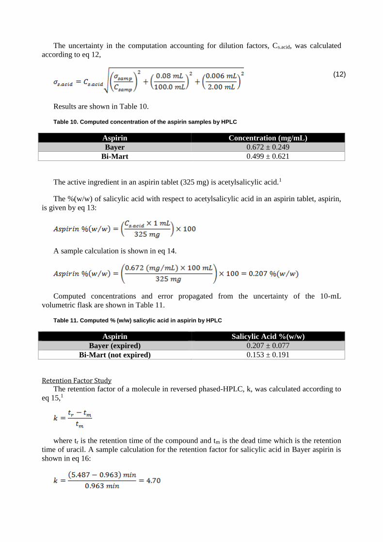
The uncertainty in the computation accounting for dilution factors, Cs.acid, was calculated
according to eq 12,
Results are shown in Table 10.
Table 10. Computed concentration of the aspirin samples by HPLC
Aspirin Concentration (mg/mL)
Bayer 0.672 ± 0.249
Bi-Mart 0.499 ± 0.621
The active ingredient in an aspirin tablet (325 mg) is acetylsalicylic acid.1
The %(w/w) of salicylic acid with respect to acetylsalicylic acid in an aspirin tablet, aspirin,
is given by eq 13:
A sample calculation is shown in eq 14.
Computed concentrations and error propagated from the uncertainty of the 10-mL
volumetric flask are shown in Table 11.
Table 11. Computed % (w/w) salicylic acid in aspirin by HPLC
Aspirin Salicylic Acid %(w/w)
Bayer (expired) 0.207 ± 0.077
Bi-Mart (not expired) 0.153 ± 0.191
Retention Factor Study The retention factor of a molecule in reversed phased-HPLC, k, was calculated according to
eq 15,1
where tr is the retention time of the compound and tm is the dead time which is the retention
time of uracil. A sample calculation for the retention factor for salicylic acid in Bayer aspirin is
shown in eq 16:
(12)
The retention factors for salicylic acid, acetylsalicylic acid, and ethyl paraben in the aspirin
separation is shown in Table 12.
Table 12. Retention factors of salicylic acid (SA), acetylsalicylic acid (ASA), and ethyl paraben (EP) in aspirin samples
Aspirin Retention Factor, k
Bayer SA 4.70
Bayer ASA 2.54
Bayer EP 7.71
Bi-Mart SA 5.17
Bi-Mart ASA 2.79
Bi-Mart EP 8.53
Resolution of Chromatographic System The resolution of the chromatographic system, Rs, using the salicylic acid and
acetylsalicylic acid peaks from the aspirin separation was calculated according to eq 17,
where (tr)B is the retention time of salicylic acid, (tr)A is the retention time of acetylsalicylic
acid, WA and WB is the width of acetylsalicylic acid and salicylic acid taken from the Bayer
sample. A sample calculation for resolution in Bayer aspirin is shown in eq 18:
The resolution calculation results are shown in Table 13.
Table 13. Resolution for chromatographic separation of salicylic acid and acetylsalicylic acid
Aspirin Resolution, Rs
Bayer 9.08
Bi-Mart 10.0
The minimum retention time difference required for complete separation is generally
accepted as an separation factor of 1.5 or greater (α).2 Retention time difference is proportional
to the resolution as shown in eq 17, calculation of minimum retention time is shown in eq 19,
Minimum retention time difference for both aspirin samples are shown in Table 14.
Sample calculation for Bayer is shown in eq 20:
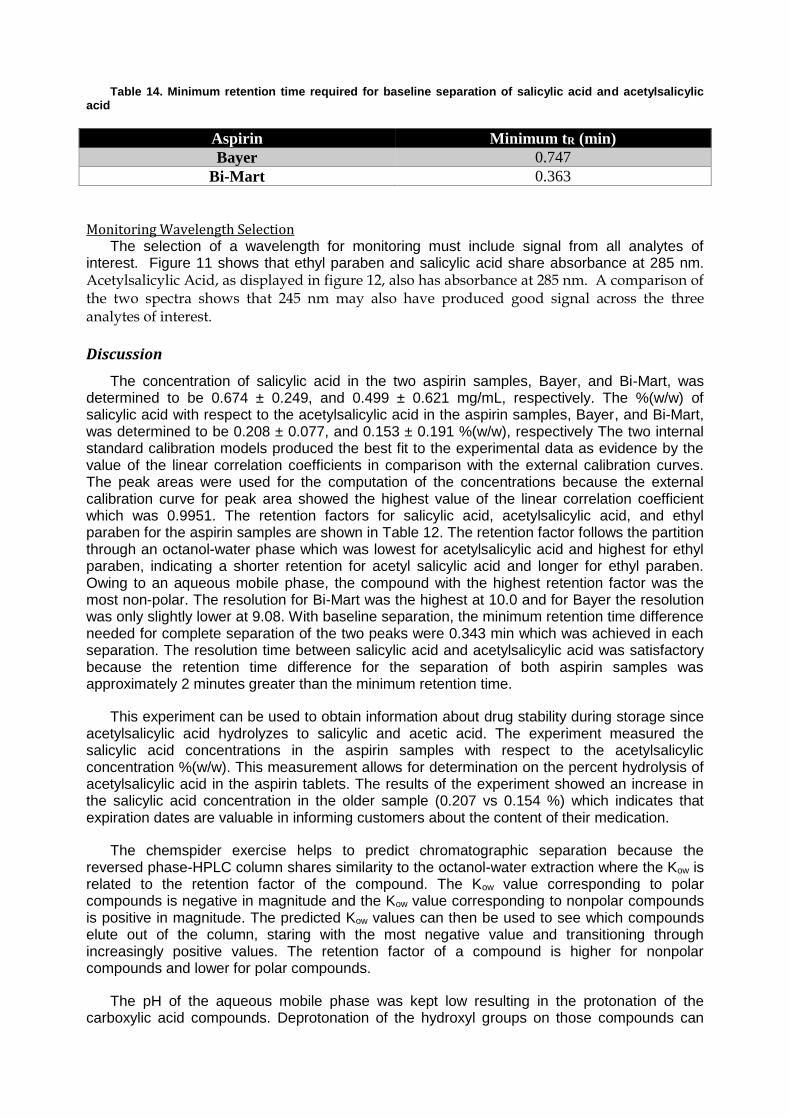
Table 14. Minimum retention time required for baseline separation of salicylic acid and acetylsalicylic acid
Aspirin Minimum tR (min)
Bayer 0.747
Bi-Mart 0.363
Monitoring Wavelength Selection The selection of a wavelength for monitoring must include signal from all analytes of
interest. Figure 11 shows that ethyl paraben and salicylic acid share absorbance at 285 nm. Acetylsalicylic Acid, as displayed in figure 12, also has absorbance at 285 nm. A comparison of the two spectra shows that 245 nm may also have produced good signal across the three analytes of interest.
Discussion
The concentration of salicylic acid in the two aspirin samples, Bayer, and Bi-Mart, was determined to be 0.674 ± 0.249, and 0.499 ± 0.621 mg/mL, respectively. The %(w/w) of salicylic acid with respect to the acetylsalicylic acid in the aspirin samples, Bayer, and Bi-Mart, was determined to be 0.208 ± 0.077, and 0.153 ± 0.191 %(w/w), respectively The two internal standard calibration models produced the best fit to the experimental data as evidence by the value of the linear correlation coefficients in comparison with the external calibration curves. The peak areas were used for the computation of the concentrations because the external calibration curve for peak area showed the highest value of the linear correlation coefficient which was 0.9951. The retention factors for salicylic acid, acetylsalicylic acid, and ethyl paraben for the aspirin samples are shown in Table 12. The retention factor follows the partition through an octanol-water phase which was lowest for acetylsalicylic acid and highest for ethyl paraben, indicating a shorter retention for acetyl salicylic acid and longer for ethyl paraben. Owing to an aqueous mobile phase, the compound with the highest retention factor was the most non-polar. The resolution for Bi-Mart was the highest at 10.0 and for Bayer the resolution was only slightly lower at 9.08. With baseline separation, the minimum retention time difference needed for complete separation of the two peaks were 0.343 min which was achieved in each separation. The resolution time between salicylic acid and acetylsalicylic acid was satisfactory because the retention time difference for the separation of both aspirin samples was approximately 2 minutes greater than the minimum retention time.
This experiment can be used to obtain information about drug stability during storage since acetylsalicylic acid hydrolyzes to salicylic and acetic acid. The experiment measured the salicylic acid concentrations in the aspirin samples with respect to the acetylsalicylic concentration %(w/w). This measurement allows for determination on the percent hydrolysis of acetylsalicylic acid in the aspirin tablets. The results of the experiment showed an increase in the salicylic acid concentration in the older sample (0.207 vs 0.154 %) which indicates that expiration dates are valuable in informing customers about the content of their medication.
The chemspider exercise helps to predict chromatographic separation because the reversed phase-HPLC column shares similarity to the octanol-water extraction where the Kow is related to the retention factor of the compound. The Kow value corresponding to polar compounds is negative in magnitude and the Kow value corresponding to nonpolar compounds is positive in magnitude. The predicted Kow values can then be used to see which compounds elute out of the column, staring with the most negative value and transitioning through increasingly positive values. The retention factor of a compound is higher for nonpolar compounds and lower for polar compounds.
The pH of the aqueous mobile phase was kept low resulting in the protonation of the carboxylic acid compounds. Deprotonation of the hydroxyl groups on those compounds can

cause the polarity of the molecule to increase, thus increasing the retention time of the compound and making separation difficult. The Kow values of the deprotonated carboxylic acid groups were more negative than uracil. Uracil is considered an unretained compound so the carboxylates would be even more unretained making separation by reversed phase-HPLC difficult at higher pH’s. Deceasing the pH even further might cause a derogation in the signal as acid-catalyzed esterification can occur on the carboxylic acid groups causing further impurities and decreasing the analyte concentration being measured.
References
4. Chemistry 426: Instrumental Analysis Laboratory Manual, Department of Chemistry,
Southern Oregon University: Ashland, OR, 2013; pp 3-19.
5. The LC Handbook: Guide to LC columns and Method Development, Agilent
Technologies. Pp 7-8.
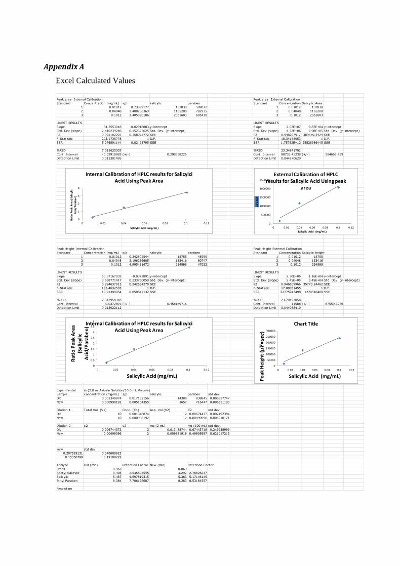
Appendix A
Excel Calculated Values
Peak area Internal Calibration Peak area External Calibration
Standard Concentration (mg/mL) s/p salicylic paraben Standard Concentration Salicylic Area
1 0.01012 0.23399177 137838 589072 1 0.01012 137838
2 0.04048 1.488256369 1165208 782935 2 0.04048 1165208
3 0.1012 3.405320186 2061683 605430 3 0.1012 2061683
LINEST RESULTS LINEST RESULTS
Slope 34.3553018 -0.02918883 y-intercept Slope 2.02E+07 9.87E+04 y-intercept
Std. Dev (slope) 2.410239246 0.152325625 Std. Dev. (y-intercept) Std. Dev (slope) 4.72E+06 2.98E+05 Std. Dev. (y-intercept)
R2 0.995102207 0.158075772 SEE R2 0.948297917 309559.3424 SEE
F-Statistic 203.1735778 1 D.F. F-Statistic 18.34158053 1 D.F.
SSR 5.076891144 0.02498795 SSE SSR 1.75762E+12 95826986445 SSE
%RSD 7.015625303 %RSD 23.34971701
Conf. Interval -0.02918883 (+/-) 0.298558226 Conf. Interval 98736.45238 (+/-) 584665.739
Detection Limit 0.013301495 Detection Limit 0.044270629
Peak Height Internal Calibration Peak Height External Calibration
Standard Concentration (mg/mL) s/p salicylic paraben Standard Concentration Salicylic height
1 0.01012 0.342805544 15755 45959 1 0.01012 15755
2 0.04048 2.196256605 133416 60747 2 0.04048 133416
3 0.1012 4.995491472 234898 47022 3 0.1012 234898
LINEST RESULTS LINEST RESULTS
Slope 50.37167932 -0.0372891 y-intercept Slope 2.30E+06 1.16E+04 y-intercept
Std. Dev (slope) 3.698771417 0.233760059 Std. Dev. (y-intercept) Std. Dev (slope) 5.45E+05 3.45E+04 Std. Dev. (y-intercept)
R2 0.994637013 0.242584278 SEE R2 0.946809966 35770.24462 SEE
F-Statistic 185.4632535 1 D.F. F-Statistic 17.80051455 1 D.F.
SSR 10.91398054 0.058847132 SSE SSR 22775943498 1279510400 SSE
%RSD 7.342958318 %RSD 23.70193058
Conf. Interval -0.0372891 (+/-) 0.458169716 Conf. Interval 11588 (+/-) 67559.3776
Detection Limit 0.013922112 Detection Limit 0.044938419
Experimental in (2.0 ml Asipirin Solution/10.0 mL Volume)
Sample concentration (mg/mL) s/p salicylic paraben std dev
Old 0.001348874 0.017152156 14388 838845 0.006337747
New 0.000998192 0.005104355 3657 716447 0.006351193
Dilution 1 Total Vol. (V1) Conc. (C1) Asp. Vol (V2) C2 std dev
Old 10 0.001348874 2 0.00674437 0.002492384
New 10 0.000998192 2 0.00499096 0.006210171
Dilution 2 c2 v2 mg (2 mL) mg (100 mL) std dev.
Old 0.006744372 2 0.013488744 0.67443718 0.249238999
New 0.00499096 2 0.009981919 0.49909597 0.621017213
w/w std dev
0.207519131 0.076688923
0.15356799 0.19108222
Analyte Old (min) Retention Factor New (min) Retention Factor
Uracil 0.963 0.869
Acetyl Salicylic 3.405 2.535825545 3.292 2.78826237
Salicylic 5.487 4.697819315 5.363 5.17146145
Ethyl Paraben 8.384 7.706126687 8.283 8.53164557
Resolution
0
1
2
3
4
0 0.02 0.04 0.06 0.08 0.1 0.12
Rat
io P
eak
Are
a (S
alic
ylic
A
cid
/Par
abe
n)
Salicylic Acid (mg/mL)
Internal Calibration of HPLC results for Salicylci Acid Using Peak Area
0
500000
1000000
1500000
2000000
2500000
0 0.02 0.04 0.06 0.08 0.1 0.12
µ ∗
Salicylic Acid (mg/mL)
External Calibration of HPLC results for Salicylic Acid Using peak
area
0
50000
100000
150000
200000
250000
300000
0 0.02 0.04 0.06 0.08 0.1 0.12
Pe
ak
He
igh
t (µ ∗
)
Salicylic Acid (mg/mL)
Chart Title
0
0.5
1
1.5
2
2.5
3
3.5
4
0 0.02 0.04 0.06 0.08 0.1 0.12
Ra
tio
Pe
ak
Are
a
(Sa
licyl
ic
Aci
d/P
ara
be
n)
Salicylic Acid (mg/mL)
Internal Calibration of HPLC results for Salicylci Acid Using Peak Area
Mark Weir Winter 2014
Determination of Copper in Brass by Atomic Absorption Spectroscopy
Introduction
In this experiment, atomic absorption spectroscopy (AAS) was performed on a sample solution with a given brass concentration. The absorbance of the sample was measured, and a linear calibration model for copper was constructed using the method of least squares at three different band-passes: 0.2, 0.5, and 1.0-nm. The calibration model was based on the absorbance produced by a series of six copper standard solutions. The calibration model was then used to determine the copper content in the sample. Further study on the instrumental parameters was conducted by measuring the absorbance of the sample and standards at different band-passes and burner heights.
Procedure
The experiment was performed according to the Chemistry 426 laboratory handout provided (Petrovic, S.C. Southern Oregon University, Ashland, OR. Atomic Absorption Spectroscopy Determination of Cu in brass, 2006).
Apparatus
The instrument used in this experiment was a Thermo Jarrell-Ash Unicam Solaar 989 Atomic Absorption Spectrometer. The standard mixtures for calibration were prepared in 100-mL volumetric flasks.
Calculations and Results
Absorbance Study The absorbance of a brass sample was analyzed at three different band-passes to compute
the mean absorbance, standard deviation of absorbance, and percent relative standard deviation (%RSD). Means and standard deviations were computed by use of statistical functions in the Microsoft Excel 2013. The data is shown in table 1, the equations for the calculation of standard deviation and %RSD.
Table 1. Absorbance of brass sample by AAS at a band-pass of 0.2, 0.5, and 1.0-nm
Band-pass (nm) Mean Absorbance Standard Deviation %RSD
0.2 0.1035 0.0003 0.29
0.5 0.1005 0.0010 0.95
1.0 0.0866 0.0013 1.50
Copper Calibration Study Concentration of the certified AAS copper standard, CCu, was 1000 ppm.
The standard copper solutions were prepared by pipetting 50.0, 100.0, 150.0, 200.0, and 250.0 µL of the certified copper standard into their respective 100-mL volumetric flasks. The concentration of any given standard, Cstd, was calculated according to eq 1,

where V is the aliquot volume in L.
Standard concentrations are shown in Table 2. A sample calculation for standard #1 is shown in eq 2:
Table 2. Calculated concentration of copper standards
Standard # Concentration (ppm)
Blank 0.000
1 0.500
2 1.000
3 1.500
4 2.000
5 2.500
Determination of copper in the brass sample requires the calculation of mean absorbance
units, standard deviations, and 95% confidence intervals for the copper standards using
Microsoft Excel. The results are shown for 0.2, 0.5, 1.0-nm band-pass on Table 3,4, and 5,
respectively.
Table 3. Quantitative results of copper determination using AAS at a band-pass of 0.2-nm
Concentration
(ppm)
Mean Absorbance Standard Deviation 95 % Confidence
Interval
0.000 0.0055 0.0005 ±0.0013
0.500 0.0343 0.0005 ±0.0012
1.000 0.0647 0.0005 ±0.0013
1.500 0.0957 0.0005 ±0.0012
2.000 0.1199 0.0011 ±0.0027
2.500 0.1502 0.0005 ±0.0013
Table 4. Quantitative results of copper determination using AAS at a band-pass of 0.5-nm
Concentration
(ppm)
Mean Absorbance Standard Deviation 95 % Confidence
Interval
0.000 0.0080 0.0006 ±0.0015
0.500 0.0381 0.0002 ±0.0005
1.000 0.0649 0.0006 ±0.0014
1.500 0.0912 0.0007 ±0.0017
2.000 0.1180 0.0012 ±0.0029
2.500 0.1455 0.0008 ±0.0021
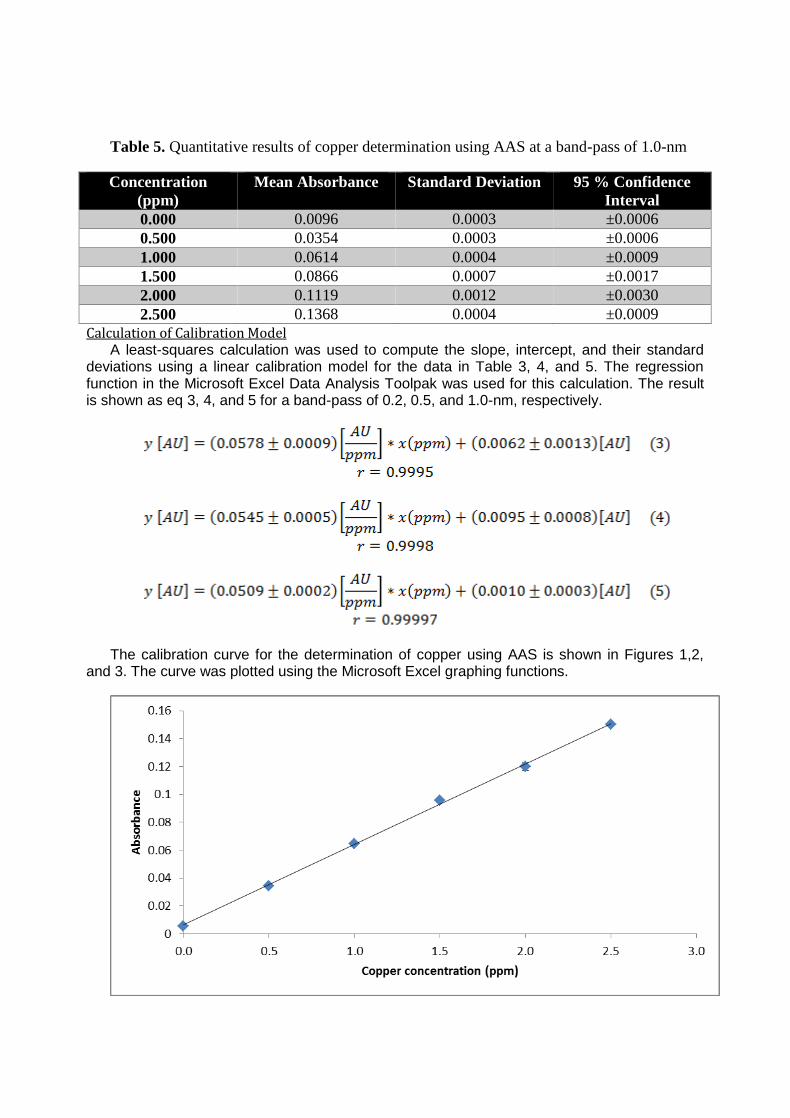
Table 5. Quantitative results of copper determination using AAS at a band-pass of 1.0-nm
Concentration
(ppm)
Mean Absorbance Standard Deviation 95 % Confidence
Interval
0.000 0.0096 0.0003 ±0.0006
0.500 0.0354 0.0003 ±0.0006
1.000 0.0614 0.0004 ±0.0009
1.500 0.0866 0.0007 ±0.0017
2.000 0.1119 0.0012 ±0.0030
2.500 0.1368 0.0004 ±0.0009
Calculation of Calibration Model A least-squares calculation was used to compute the slope, intercept, and their standard
deviations using a linear calibration model for the data in Table 3, 4, and 5. The regression function in the Microsoft Excel Data Analysis Toolpak was used for this calculation. The result is shown as eq 3, 4, and 5 for a band-pass of 0.2, 0.5, and 1.0-nm, respectively.
The calibration curve for the determination of copper using AAS is shown in Figures 1,2, and 3. The curve was plotted using the Microsoft Excel graphing functions.

Figure 1. AAS calibration data at 0.2-nm bandpass for the determination of copper in the
brass sample. The line, which is the line of best fit, is y = 0.0578x + 0.0062 where x is the
copper concentration in ppm and y is the absorbance. Error bars indicate 95% confidence
intervals.
Figure 2. AAS calibration data at 0.5-nm bandpass for the determination of copper in the
brass sample. The line, which is the line of best fit, is y = 0.0545x + 0.0095 where x is the
copper concentration in ppm and y is the absorbance. Error bars indicate 95% confidence
intervals.
Figure 3. AAS calibration data at 1.0-nm bandpass for the determination of copper in the
brass sample. The line, which is the line of best fit, is y = 0.0509x + 0.0100 where x is the

copper concentration in ppm and y is the absorbance. Error bars indicate 95% confidence
intervals.
Calculation of the detection limit (DL) for any of the calibration curves is shown in eq 6,
where Sb is the standard deviation of the y-intercepy and m is the slope.
Detection limits are shown in Table 6. A sample calculation at a band-pass of 0.2-nm is
shown in eq 7:
Table 6. Calculated detection limits of the three calibration curves
Bandpass (nm) Detection Limit (ppm)
0.2 0.320
0.5 0.521
1.0 0.587
Computation of Copper Concentration in Brass Sample at 0.2-nm band-pass
The mean absorbance of the brass sample was calculated to be 0.0981. The value was used
with the computed slope and intercept (eq 3) to determine the concentration of copper in the
brass sample as shown in eq 6.
The 95% confidence interval was calculated to be ±0.064 ppm.
The sample being measured had an original brass concentration of 0.5035 g/L, but a 1000.0
µL was aliquoted into a 250-mL volumetric flask. Calculation of the concentration of the brass
sample, Cbrass, is shown below in eq 7.
Calculation of the concentration of the original brass sample expressed as %(w/w) is shown
in eq 7:
The 95% confidence interval was calculated to be ±3.18 %(w/w) Cu.
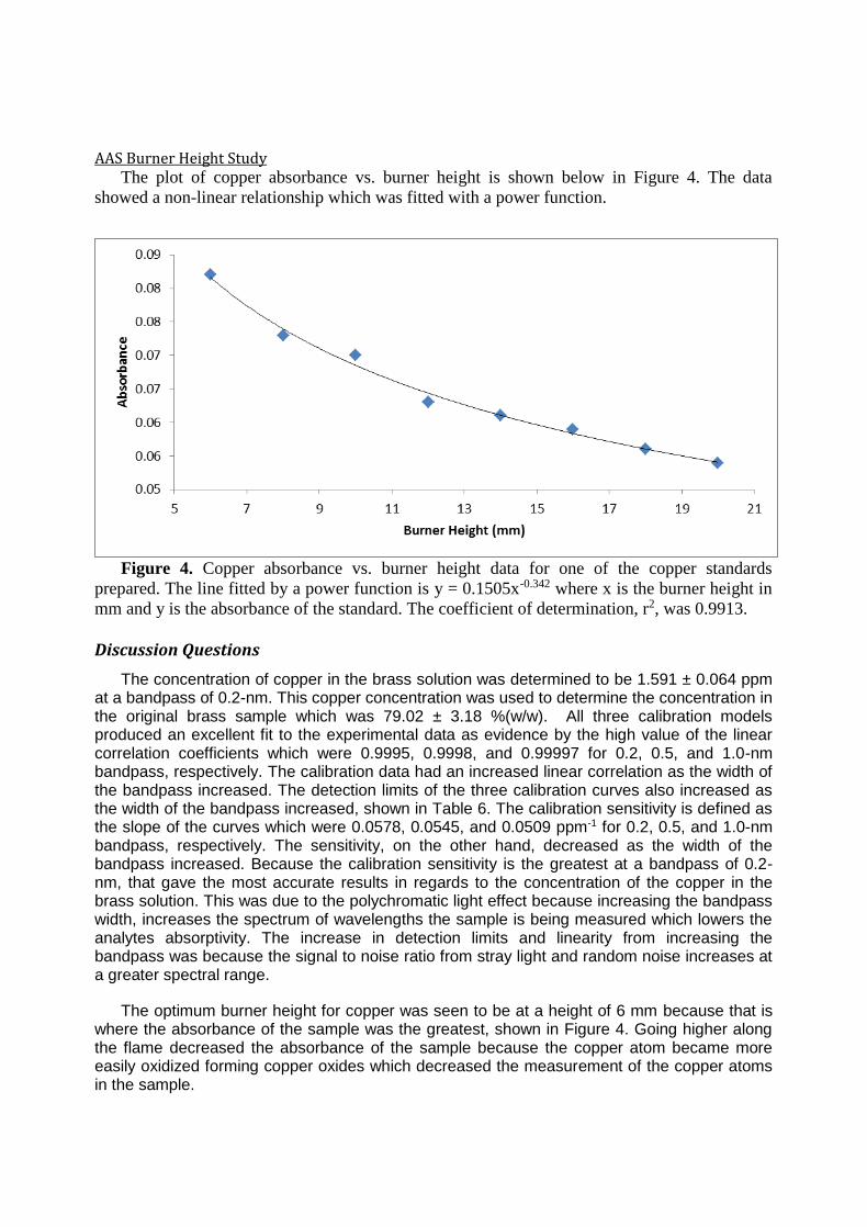
AAS Burner Height Study The plot of copper absorbance vs. burner height is shown below in Figure 4. The data
showed a non-linear relationship which was fitted with a power function.
Figure 4. Copper absorbance vs. burner height data for one of the copper standards
prepared. The line fitted by a power function is y = 0.1505x-0.342 where x is the burner height in
mm and y is the absorbance of the standard. The coefficient of determination, r2, was 0.9913.
Discussion Questions
The concentration of copper in the brass solution was determined to be 1.591 ± 0.064 ppm at a bandpass of 0.2-nm. This copper concentration was used to determine the concentration in the original brass sample which was 79.02 ± 3.18 %(w/w). All three calibration models produced an excellent fit to the experimental data as evidence by the high value of the linear correlation coefficients which were 0.9995, 0.9998, and 0.99997 for 0.2, 0.5, and 1.0-nm bandpass, respectively. The calibration data had an increased linear correlation as the width of the bandpass increased. The detection limits of the three calibration curves also increased as the width of the bandpass increased, shown in Table 6. The calibration sensitivity is defined as the slope of the curves which were 0.0578, 0.0545, and 0.0509 ppm-1 for 0.2, 0.5, and 1.0-nm bandpass, respectively. The sensitivity, on the other hand, decreased as the width of the bandpass increased. Because the calibration sensitivity is the greatest at a bandpass of 0.2-nm, that gave the most accurate results in regards to the concentration of the copper in the brass solution. This was due to the polychromatic light effect because increasing the bandpass width, increases the spectrum of wavelengths the sample is being measured which lowers the analytes absorptivity. The increase in detection limits and linearity from increasing the bandpass was because the signal to noise ratio from stray light and random noise increases at a greater spectral range.
The optimum burner height for copper was seen to be at a height of 6 mm because that is where the absorbance of the sample was the greatest, shown in Figure 4. Going higher along the flame decreased the absorbance of the sample because the copper atom became more easily oxidized forming copper oxides which decreased the measurement of the copper atoms in the sample.

A blank was necessary because of the fuel or oxidant which would show up as absorbance measurements from refractory compound formations. A 2% HNO3 blank was used instead of distilled water because of chemical interferences. The matrix of the solution needs to match in each standard as well as the blank and since the sample of the brass solution was dissolved in nitric acid, the blank needs to match the standards. Also, the interaction of the copper ion in a nitric acid solution makes it preferable over distilled water because nitric acid complexes with the copper ions in solution.
Reference
6. Chemistry 426: Instrumental Analysis Laboratory Manual, Department of Chemistry,
Southern Oregon University: Ashland, OR, 2013; pp 45-48.
Mark Weir December 8, 2013
Constituents of Lithia Water
Introduction
At the turn of the 20th century, emergent cities throughout the Pacific Northwest were looking for new ways to attract tourists and expand their economic base. Fading gold discoveries as early as the 1880’s and an increased economic competiveness along the north-south rail lines of Oregon meant that smaller communities, absent of major ports or agricultural bases, needed to develop on the natural resources present throughout the Siskiyou-Cascade ranges. The community of Ashland Oregon, established during the mid-19thcentury, was one such base, which sought to develop natural resources with national appeal. During the early 1900’s, water springs, especially those high in mineral Lithium, were considered to have
significant healing capabilities 1 Used since the 1870’s to treat mania, digestive problems,
arthritis, and rheumatism, the product was only limitedly developed by drug companies since,
as a naturally occurring mineral, it could not be patented.2 This allowed communities with high
concentrations of Lithium or other minerals in local springs, such as Ashland, to market the healing waters as a tourist attraction and purchasable bottled drinking water. Today, Lithium water and the history of its development in Ashland are the story of a community focused on expanding its use of natural resources, albeit not always in the way or to the full effect city planners had hoped.
The Pompadour Chief Springs, located approximately 4 miles southeast of Ashland and named for the bluff from which it flowed, was long known to the Modoc, Shasta, Tekelma, Latgawa and Umpqua tribes, the indigenous populations of Jackson county, for its ability to
provide restorative sensations3 By 1909 the springs in Ashland had become so well known
that C. B. Watson included them in his seminal discussion of the Siskiyou Mountains.4
Development of the Lithia springs, not to be confused with other white sulfur springs which already existed in Ashland, was conducted by H. Silver and G. H. Gillette after their purchase
of the property in 1907 1 Mr. Silver improved the property as a spa location but also sold his
brand of Lithia water nationwide and franchised the rights for the bottling of CO2 to the Liquid Carbonic Company of Chicago, IL which operated a CO2 capture facility on the property until
1929.1 Interestingly, the Silver wells did not provide the original Lithia water pumped to the
downtown of Ashland as the city was forced to use a nearby well to initially supply the town
because of competing interest between Mr. Silver and other city planners 1 It was not until
1929, when the city acquired the Silver property in foreclosure, that the primary spring was
moved from the city’s adjacent property.1
Perhaps one of the greatest proponents of developing Ashland via exploitation of the nearby Lithia water was the owner of the Daily Tidings and Commercial Club member, Bert
Greer.5 Around 1913 he put forth an ambitious plan to pump water from the springs to
downtown Ashland in an effort to create unique economic opportunities.1 Greer and fellow
enthusiasts looked to expand Ashland’s national image as a health spa destination through the
development of a number of tourist hotels and sanitariums1 The city voted in 1914 to approve
a bond for $175,000 for the development of the resource and to bring Lithia water to the town
and the newly developed Lithia Park.1 To bolster the claims of Lithia water advocates the city
also commissioned an in-depth mineral analysis of the water, quantifying the composition of the water in an attempt to provide numeric support for minerals present. Numerous bath houses attempted to capitalize on Ashland’s economic drive to become a health resort destination including the once famous Natatorim Sulphur Baths, later known as the Twin Plunges and
located in what is now the historic rail road district and the Helman Sulpher Baths, where many
Ashland residents learned to swim.5 Additionally, many entrepreneurs bottled and sold the later
with estimated cases sold ranging from 12,000 to over 100,000.1 Unfortunately for many of
these establishments, the collective economic hit of World War I (1914-1918), the Great Depression and the transition of the rail road’s north-south route through Klamath Falls greatly
reduced tourism to Ashland through the midcentury 5
Although the springs were long touted as having medicinal properties, the claims are historically considered an over exaggeration, driven in large part by the work of Mr. Greer, the owner of the local newspaper. Recent commentary by psychiatrist Dr. Mark Bradsaw indicate that a person would need to consume between 100 and 150 Liters of Lithia water a day to
achieve dosages prescribed for medical treatment.6 Given the number of ancillary constituents
present in the water, many of which impart a less than desirable drinking quality, it is hard to imagine individuals willing to consume levels to achieve the desired effect. In this way, the development of Lithia water at the turn of the century was akin to the selling of snake oils prevalent before the enactment of the 1906 Food and Drugs act which resulted in the
requirement that claims be substantiated 7
Building on the local history of rejuvenating waters, present day hotels such as the Lithia Springs Resort in North Ashland continues to offer personalized in room spring baths which are
purported to “relieve soreness or irritation”, although these are all sulfur springs.8 Additionally,
the Ashland Springs hotel (formerly the Lithia Springs Hotel), the largest building in downtown
Ashland and a historic landmark, derives its name from Ashland’s history with spring water.1
Ashland’s historic central park, Lithia Park, developed at the same time as the springs,
acquired its name in an endeavor to promote the water.1 Fountains situated at the front of the
park in the Ashland Plaza continue to bring Lithia water from the spring much to the chagrin of tourist unfamiliar with the distinct taste. Although the concentrations of Lithium in the water (6.71 mg L-1) are far below the doses commonly prescribed for medical treatment (1,200 mg
day-1), visitors can often be seen tempting each other to try the foul smelling water.6
Undoubtedly, the presence, development, and marketing of Lithia water played an important role in the expansion of Ashland. Although many of the early claims and hopes of businesses in Ashland who looked to capitalize on the water were never fully realized, the historic impact of the water is difficult to understate.
Procedure
Sampling Initial samples were taken on the 21st of October 2013 and one sample (~125 mL) was
stabilized with 3.0 mL of 16 M Nitric acid (HNO3) to prevent iron oxidation and stored at 4 °C. The second sample (1000 mL) was tightly closed and was stored at 4 °C with no further treatment. Aliquots from the 1 Liter sample were used for all experimentation. Analysis, by way of H+ ion selective electrode (ISE) at the SOU laboratory indicated the Lithia water samples had an initial pH of 6.25. Further, the iron sample had a pH of 0.65 upon addition of Nitric acid, suggesting appropriate H+ concentration for achievement of stabilization.
Determination of Bicarbonate in Lithia Water A waters ability to neutralize acid is known as its alkalinity. In a majority of waterways the
total alkalinity it’s due solely to bicarbonate. The alkalinity and thus the bicarbonate content of a water source is determined by titration with a strong acid. In order to determine the end point of the titration and the amount of acid used, there are two indicators, phenolphthalein and bromocresol. Titrating to the phenolphthalein endpoint of pH 8.3 determines the phenolphthalein alkalinity and the end-point by means of bromocresol indicator determines total alkalinity. Phenolphthalein is bright pink under basic conditions and turns clear under acidic conditions at a pH of 8.3. Bromocresol at higher pH levels is fully deprotonated and in this dianionic form it takes its common blue color. However, at lower pH, approximately 4.8, it turns a bright yellow. Both the pink to white and blue to yellow endpoints are what indicate the
titration has been completed. Free carbon dioxide is a common interference and thus previous to the titration the sample is boiled to remove from the sample.
Determination of Ferrous Iron in Lithia Water Waterways contain only minor concentrations of iron, though in the earth’s crust the
elemental form is fairly abundant. This is due to free iron in waterways linked dependence on the pH of the water. Iron is commonly found in two states. The ferrous form (Fe2+) is relatively soluble in water; however, the ferric form (Fe3+) is highly insoluble and precipitates out of solution. Only at a pH below 3 does ferric iron convert to the ferrous form and dissolve into solution. In order to accurately measure the total iron content of Lithia water, the sample was reduced and subsequently the pH was lowered to less than 2. This ceased the oxidative process and converted all forms of iron to the ferrous form. Total iron content was determined via photometric spectroscopy where iron was bound to 1, 10-phenanthroline. This chelation forms a red-orange complex proportional to the concentration of iron. The complex color is measured at 510 nm and by use of Beer’s law the iron content was determined based on sample absorbance.
Determination of Chloride in Lithia Water Of the analytes of interest in Lithia water, chloride is one of the few that can be determined
by precipitation titrations. The presence of chloride in quantities of thousands of mg per Liter make it ideal for analysis using the Fajan method. In this method, a known concentration of silver nitrate is used to titrate water containing chloride in the presence of a weakly acidic indicator dye known as dichlorofluorescein. As the equivalence point is reached, small colloidal silver precipitants form and become attracted to the negatively changed dye, causing the solution to go from yellow to pink. Calculations of the total chloride are conducted by accounting for the stoichiometric relationship of one silver per chloride in the insolvent silver chloride salt. Owing to the possible formation of similar salt formation among other column seven halogens, such as bromide and iodide, it is important to ensure that these ions are not present. Historically neither has been described as a major component of Lithia water.
Determination of Calcium and Magnesium in Lithia Water Determination of the concentrations of calcium and magnesium in a sample of Lithia water
was done by complexometric titration with ethylenediaminetetraacetic acid (EDTA). The molecule EDTA is a titrant that forms a stable complex with multivalent electrons in solution via four carboxylic acid groups and non-bonded lone pairs. When combined with an indicator such as eriochrome black T, EDTA can be used to titrate a solution to a clear end point. While it is very effective, EDTA is a non-specific titrant that will complex with all multivalent cations in solution; therefore it is necessary to titrate in two steps. First the initial solution was titrated to determine the “total hardness”, the magnesium ions were then precipitated out by adding a base. The calcium content was determined with an additional titration and the difference was the magnesium content.
Determination of Sodium and Lithium in Lithia Water Analysis of the concentration of sodium in Lithia water was done using inductively coupled
plasma emission spectroscopy. Inductively coupled plasma optical emission spectroscopy (ICP-OES) is a technique with sensitivity in the range of parts per billion. This technique is ideal for the determination of mineral species in water. The analyte is vaporized followed by the excitation of the nuclei upon contact with the ionized argon plasma. As the analyte nuclei fall back to ground state radiation is emitted and absorbed by a photo array, which records the signal intensity. A multi-point calibration curve was constructed using three solutions of known concentrations to minimize error. The sample ran and the resulting intensity was applied to the equation for the line of best fit, yielding the concentration of the original sample. The results for the lithium and sodium determinations are recorded in Table1.
Determination of Potassium in Lithia Water
The concentration of potassium in Lithia water was determined by an ion specific electrode. In this technique a potassium specific electrode was used to measure the activity of potassium and convert it into a potential that could be measured by a voltmeter. The potassium specific electrode activity was then compared to a standard glass reference electrode. Three potassium standards were prepared and the activity of each was analyzed, using this data a calibration curve was created with mV as a function of log concentration. A Nerst response was confirmed by having a slope of -50.75 for the linear fit. The activity of the Lithia water sample was then used to calculate the potassium concentration of the solution. This data is summarized in Table 1.
Determination of Sulfate in Lithia Water Determination of sulfate in Lithia water is primarily an endeavor in analyzing trace
substance using spectrophotometric analysis. The adapted method, an alteration of EPA method 9038, employs a turbidimetric determination of the barium sulfate salt which is
insoluble.9 The primary adaptation employed was a pretreatment of the sample with 6 N HCl to
evolve bicarbonate and passing the Lithia water through an ion exchange column to remove divalent metal ions. Measurement of transmittance at 420 nm of a set of known standards was used to create a linear model for applying Beer’s law. Application of the method is complicated by the time and mixing dependence for proper color development. However, despite these limitations, the lower limit of the method at 0.05 mmol L-1 does allow for trace quantity determination and based upon multiple parallel runs, increased confidence in the accuracy of results.
Determination of Metaborate in Lithia Water Concentrations of metaborate at the levels historically described for Lithia water (209 mg L-
1) are indicative for high boron in the igneous rocks through which the water flows to reach the surface. Analysis was conducted using the United Nations Environmental Program procedure for boron measurement which involves acidifying a sample to release any bicarbonate and then removing divalent ions using an ion exchange column similar to the method employed for
sulfate10 Boron is then reacted with curcumin resulting in a characteristic red-colored product
known as rosocyanin. This product is highly soluble in ethanol and the absorbance can be compared to standards using spectrophotometric analysis at 540 nm and Beer’s law. The drying procedure was conducted in polyethylene containers to reduce contamination from boron present in most common glassware and may have suffered from overnight storage of the rosocyanin mixture, which is unstable over extended timeframes.
Determination of Silicate in Lithia Water Silica is the second most abundant element in the earth’s crust. It is also one of the most
complex families of materials, found commonly as quarts. Even though, it is in high supply as a solid, silica is not readily soluble. The breakdown of amorphous rock by weathering is believed to be the major cause of silica found in water systems. The Lithia water sample still had to be stored in polypropylene bottles and experimental equipment was to be polypropylene as well. Ammonium molybdate at pH 1.2 reacts with the free silica and phosphorous in solution. Oxalic acid breaks down the molybdophosphoric acid but retains the molybdosilicic acid, which is reacted with aminonaptholsulphonic acid creating heteropoly blue. The reacted form of silica is determined by the spectroscopic analysis of the absorbance of set standards and the Lithia sample. Absorbance is measured at 815 nm to ensure the most accurate results.
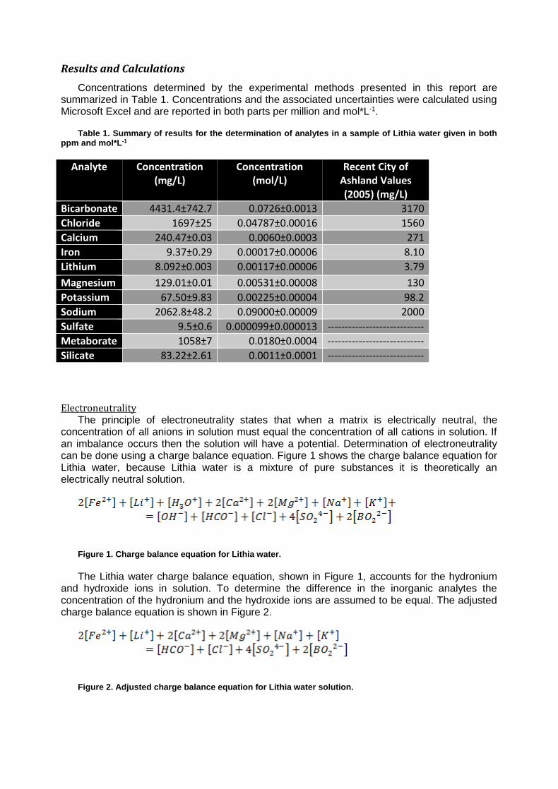
Results and Calculations
Concentrations determined by the experimental methods presented in this report are summarized in Table 1. Concentrations and the associated uncertainties were calculated using Microsoft Excel and are reported in both parts per million and mol*L-1.
Table 1. Summary of results for the determination of analytes in a sample of Lithia water given in both ppm and mol*L-1
Analyte Concentration (mg/L)
Concentration (mol/L)
Recent City of Ashland Values (2005) (mg/L)
Bicarbonate 4431.4±742.7 0.0726±0.0013 3170
Chloride 1697±25 0.04787±0.00016 1560
Calcium 240.47±0.03 0.0060±0.0003 271
Iron 9.37±0.29 0.00017±0.00006 8.10
Lithium 8.092±0.003 0.00117±0.00006 3.79
Magnesium 129.01±0.01 0.00531±0.00008 130
Potassium 67.50±9.83 0.00225±0.00004 98.2
Sodium 2062.8±48.2 0.09000±0.00009 2000
Sulfate 9.5±0.6 0.000099±0.000013 ----------------------------
Metaborate 1058±7 0.0180±0.0004 ----------------------------
Silicate 83.22±2.61 0.0011±0.0001 ----------------------------
Electroneutrality The principle of electroneutrality states that when a matrix is electrically neutral, the
concentration of all anions in solution must equal the concentration of all cations in solution. If an imbalance occurs then the solution will have a potential. Determination of electroneutrality can be done using a charge balance equation. Figure 1 shows the charge balance equation for Lithia water, because Lithia water is a mixture of pure substances it is theoretically an electrically neutral solution.
Figure 1. Charge balance equation for Lithia water.
The Lithia water charge balance equation, shown in Figure 1, accounts for the hydronium and hydroxide ions in solution. To determine the difference in the inorganic analytes the concentration of the hydronium and the hydroxide ions are assumed to be equal. The adjusted charge balance equation is shown in Figure 2.
Figure 2. Adjusted charge balance equation for Lithia water solution.

The experimentally determined values summarized in Table 1 can be used to determine the electroneutrality of the Lithia sample tested in this research, the appropriate calculation in ppm are shown in Equation 1.
(1)
To determine if there was a statistically significant difference in the concentrations of the anions and cations the uncertainty of the charge balance equation was calculated the corresponding calculations are displayed in Equation 2.
(2)
Statistical Analysis Statistical determination of the difference in cations and anions in a solution of Lithia water
was performed. An F test was used to compare the variances of the cations and anions; this is shown in Equation 3.
(3)
The null hypothesis was accepted for the F-test suggesting that there was not a significant difference in the two variances; therefore, a two-sample t-test for equal variances was performed to determine if a statistical difference in the concentrations of the cations and anions was present. The calculations and the results are shown in Figure 4, and reported at a 95 % confidence.
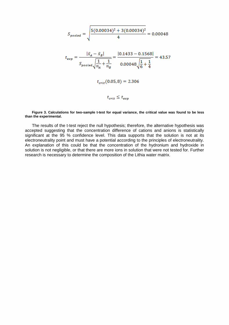
Figure 3. Calculations for two-sample t-test for equal variance, the critical value was found to be less than the experimental.
The results of the t-test reject the null hypothesis; therefore, the alternative hypothesis was accepted suggesting that the concentration difference of cations and anions is statistically significant at the 95 % confidence level. This data supports that the solution is not at its electroneutrality point and must have a potential according to the principles of electroneutrality. An explanation of this could be that the concentration of the hydronium and hydroxide in solution is not negligible, or that there are more ions in solution that were not tested for. Further research is necessary to determine the composition of the Lithia water matrix.
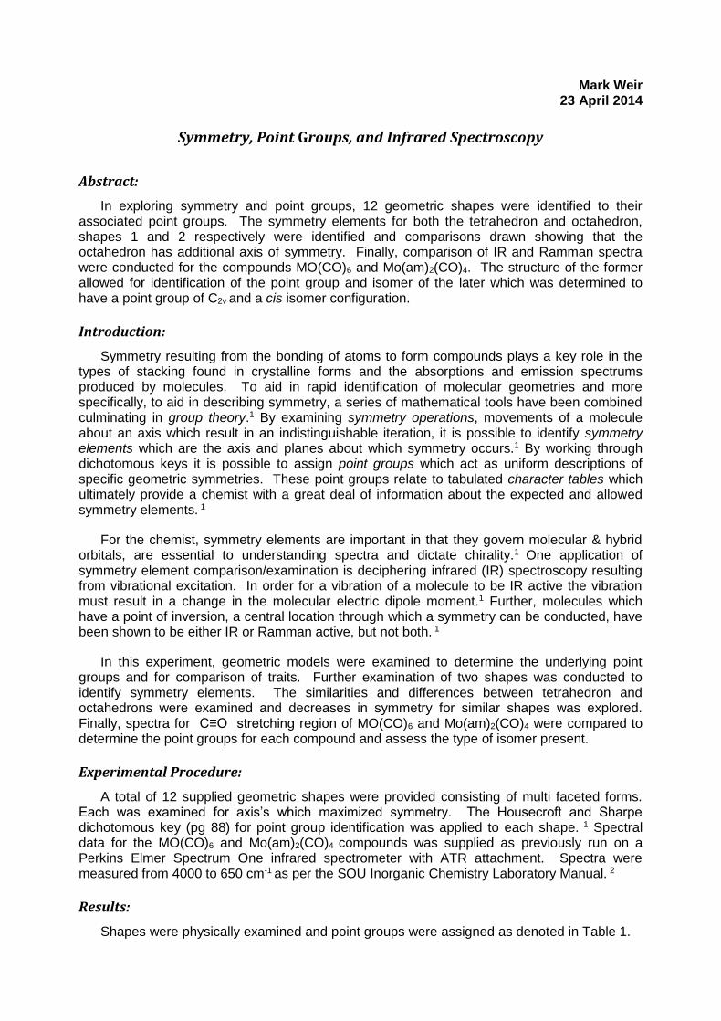
Mark Weir 23 April 2014
Symmetry, Point Groups, and Infrared Spectroscopy
Abstract:
In exploring symmetry and point groups, 12 geometric shapes were identified to their associated point groups. The symmetry elements for both the tetrahedron and octahedron, shapes 1 and 2 respectively were identified and comparisons drawn showing that the octahedron has additional axis of symmetry. Finally, comparison of IR and Ramman spectra were conducted for the compounds MO(CO)6 and Mo(am)2(CO)4. The structure of the former allowed for identification of the point group and isomer of the later which was determined to have a point group of C2v and a cis isomer configuration.
Introduction:
Symmetry resulting from the bonding of atoms to form compounds plays a key role in the types of stacking found in crystalline forms and the absorptions and emission spectrums produced by molecules. To aid in rapid identification of molecular geometries and more specifically, to aid in describing symmetry, a series of mathematical tools have been combined culminating in group theory.1 By examining symmetry operations, movements of a molecule about an axis which result in an indistinguishable iteration, it is possible to identify symmetry elements which are the axis and planes about which symmetry occurs.1 By working through dichotomous keys it is possible to assign point groups which act as uniform descriptions of specific geometric symmetries. These point groups relate to tabulated character tables which ultimately provide a chemist with a great deal of information about the expected and allowed symmetry elements. 1
For the chemist, symmetry elements are important in that they govern molecular & hybrid orbitals, are essential to understanding spectra and dictate chirality.1 One application of symmetry element comparison/examination is deciphering infrared (IR) spectroscopy resulting from vibrational excitation. In order for a vibration of a molecule to be IR active the vibration must result in a change in the molecular electric dipole moment.1 Further, molecules which have a point of inversion, a central location through which a symmetry can be conducted, have been shown to be either IR or Ramman active, but not both. 1
In this experiment, geometric models were examined to determine the underlying point groups and for comparison of traits. Further examination of two shapes was conducted to identify symmetry elements. The similarities and differences between tetrahedron and octahedrons were examined and decreases in symmetry for similar shapes was explored. Finally, spectra for C≡O stretching region of MO(CO)6 and Mo(am)2(CO)4 were compared to determine the point groups for each compound and assess the type of isomer present.
Experimental Procedure:
A total of 12 supplied geometric shapes were provided consisting of multi faceted forms. Each was examined for axis’s which maximized symmetry. The Housecroft and Sharpe dichotomous key (pg 88) for point group identification was applied to each shape. 1 Spectral data for the MO(CO)6 and Mo(am)2(CO)4 compounds was supplied as previously run on a Perkins Elmer Spectrum One infrared spectrometer with ATR attachment. Spectra were measured from 4000 to 650 cm-1 as per the SOU Inorganic Chemistry Laboratory Manual. 2
Results:
Shapes were physically examined and point groups were assigned as denoted in Table 1.
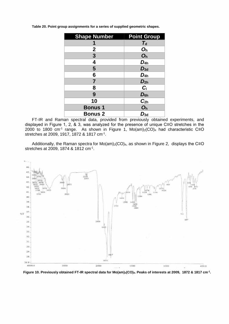
Table 20. Point group assignments for a series of supplied geometric shapes.
Shape Number Point Group
1 Td
2 Oh
3 Oh
4 D4h
5 D3d
6 D4h
7 D2h
8 Ci
9 D6h
10 C2h
Bonus 1 Oh
Bonus 2 D3d FT-IR and Raman spectral data, provided from previously obtained experiments, and
displayed in Figure 1, 2, & 3, was analyzed for the presence of unique C≡O stretches in the 2000 to 1800 cm-1 range. As shown in Figure 1, Mo(am)2(CO)4 had characteristic C≡O stretches at 2009, 1917, 1872 & 1817 cm-1.
Additionally, the Raman spectra for Mo(am)2(CO)4, as shown in Figure 2, displays the C≡O stretches at 2009, 1874 & 1812 cm-1.
Figure 10. Previously obtained FT-IR spectral data for Mo(am)2(CO)4. Peaks of interests at 2009, 1872 & 1817 cm-1.
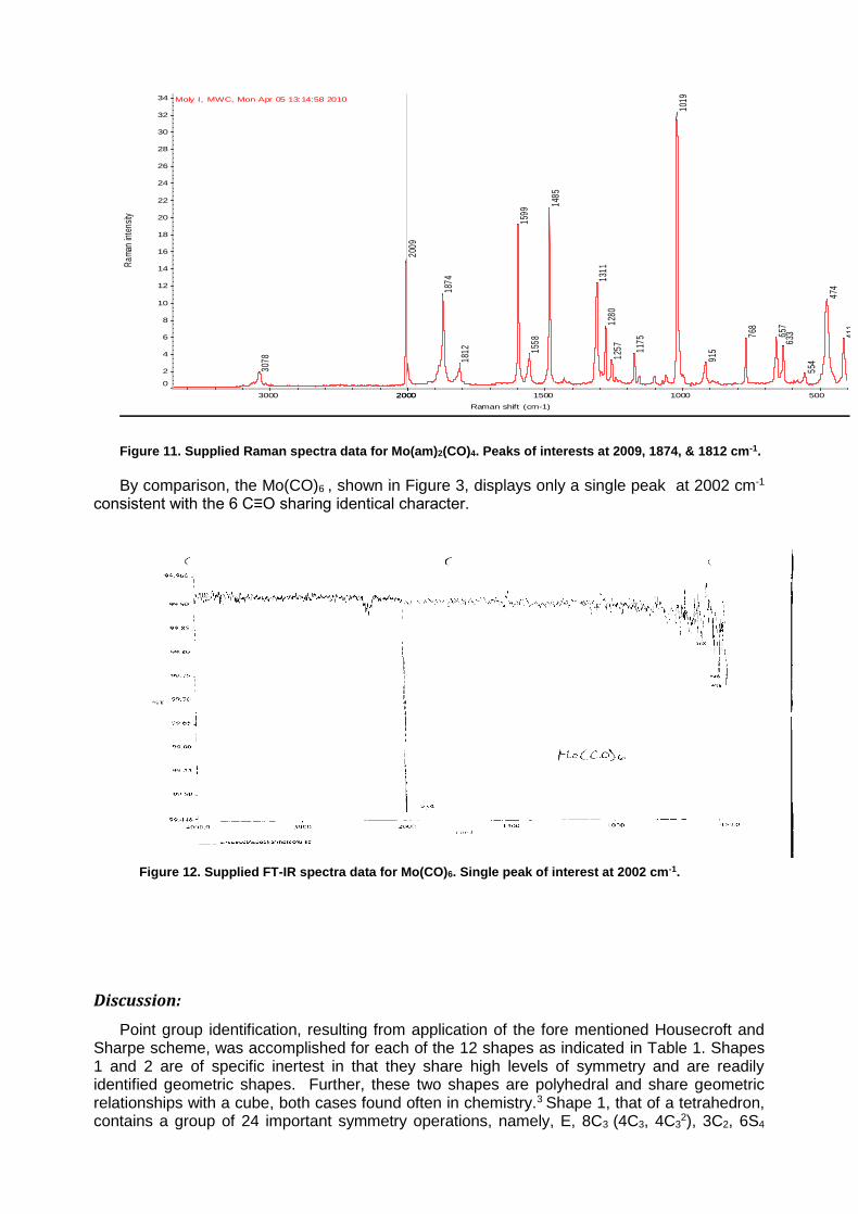
411
474
554
63365
7
768
915
1019
1175
1257
1280
1311
1485
1558
1599
1812
1874
2009
3078
Moly I, MWC, Mon Apr 05 13:14:58 2010
0
2
4
6
8
10
12
14
16
18
20
22
24
26
28
30
32
34
Ram
an in
tens
ity
500 1000 1500 2000 2000 3000
Raman shift (cm-1)
Figure 11. Supplied Raman spectra data for Mo(am)2(CO)4. Peaks of interests at 2009, 1874, & 1812 cm-1.
By comparison, the Mo(CO)6 , shown in Figure 3, displays only a single peak at 2002 cm-1 consistent with the 6 C≡O sharing identical character.
Discussion:
Point group identification, resulting from application of the fore mentioned Housecroft and Sharpe scheme, was accomplished for each of the 12 shapes as indicated in Table 1. Shapes 1 and 2 are of specific inertest in that they share high levels of symmetry and are readily identified geometric shapes. Further, these two shapes are polyhedral and share geometric relationships with a cube, both cases found often in chemistry.3 Shape 1, that of a tetrahedron, contains a group of 24 important symmetry operations, namely, E, 8C3 (4C3, 4C3
2), 3C2, 6S4
Figure 12. Supplied FT-IR spectra data for Mo(CO)6. Single peak of interest at 2002 cm-1.
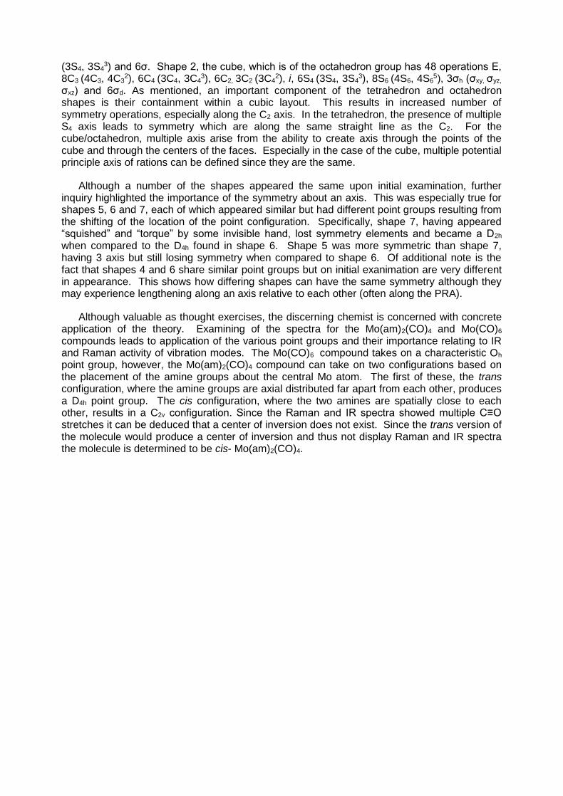
(3S4, 3S43) and 6σ. Shape 2, the cube, which is of the octahedron group has 48 operations E,
8C3 (4C3, 4C32), 6C4 (3C4, 3C4
3), 6C2, 3C2 (3C42), i, 6S4 (3S4, 3S4
3), 8S6 (4S6, 4S65), 3σh (σxy, σyz,
σxz) and 6σd. As mentioned, an important component of the tetrahedron and octahedron shapes is their containment within a cubic layout. This results in increased number of symmetry operations, especially along the C2 axis. In the tetrahedron, the presence of multiple S4 axis leads to symmetry which are along the same straight line as the C2. For the cube/octahedron, multiple axis arise from the ability to create axis through the points of the cube and through the centers of the faces. Especially in the case of the cube, multiple potential principle axis of rations can be defined since they are the same.
Although a number of the shapes appeared the same upon initial examination, further inquiry highlighted the importance of the symmetry about an axis. This was especially true for shapes 5, 6 and 7, each of which appeared similar but had different point groups resulting from the shifting of the location of the point configuration. Specifically, shape 7, having appeared “squished” and “torque” by some invisible hand, lost symmetry elements and became a D2h when compared to the D4h found in shape 6. Shape 5 was more symmetric than shape 7, having 3 axis but still losing symmetry when compared to shape 6. Of additional note is the fact that shapes 4 and 6 share similar point groups but on initial exanimation are very different in appearance. This shows how differing shapes can have the same symmetry although they may experience lengthening along an axis relative to each other (often along the PRA).
Although valuable as thought exercises, the discerning chemist is concerned with concrete application of the theory. Examining of the spectra for the Mo(am)2(CO)4 and Mo(CO)6 compounds leads to application of the various point groups and their importance relating to IR and Raman activity of vibration modes. The Mo(CO)6 compound takes on a characteristic Oh point group, however, the Mo(am)2(CO)4 compound can take on two configurations based on the placement of the amine groups about the central Mo atom. The first of these, the trans configuration, where the amine groups are axial distributed far apart from each other, produces a D4h point group. The cis configuration, where the two amines are spatially close to each other, results in a C2v configuration. Since the Raman and IR spectra showed multiple C≡O stretches it can be deduced that a center of inversion does not exist. Since the trans version of the molecule would produce a center of inversion and thus not display Raman and IR spectra the molecule is determined to be cis- Mo(am)2(CO)4.

Works Cited
1. Housecroft, Catherine and Sharpe, Alan. Inorganic Chemistry. Second. Essex, England :
Pearson Education limited, 2005.
2. Hughes, Laura. Inorganic Chemistry Laboratory. Ashland, OR : Southern Oregon
University, 2014.
3. University of Massachusetts Boston. Molecular Geometry and Point Groups. University of
Massachuesetts Boston Chemistry. [Online] [Cited: April 21, 2014.]
alpha.chem.umb.edu/chemistry/ch612/documents/moleculargeometryandpointgroups_002.pdf.

Mark Weir Winter 2013
Effects of Varied Nitrogen Treatments on Growth and Physiology among
Raphanus sativus
Introduction
The manner in which plants grow and assimilate carbon as a result of varying nutrient inputs can be illustrative in the underlying function of various physiological and anatomical features. This is especially true for the macro nutrient nitrogen which is instrumental in the carbon capture pathways of photosynthesis. In C3 plants such as Triticum aestvum L (wheat), leaf nitrogen allocation is predominately associated with photosynthesis where 18.9% is directly linked to light harvesting and 26% is committed to CO2 fixation (see figure 1). Chapin et al. have suggested that as high as 75% of leaf nitrogen in a C3 plant may be apportioned to photosynthesis in one way or another. In a strong corollary, multiple studies have identified significant links between leaf nitrogen concentrations and the photosynthetic capacity for affixing carbon. In the carbon assimilation pathway, this is especially evident among the enzyme ribulose-1,5-bisphosphate carboxylase-oxygenase which has been shown to be a highly limiting under nitrogen strain.
Research conducted by Chapin, Shaver and Kedroski has shown that nitrogen levels can also affect how plants use their assimilated carbon. The research of Chapin et al. has shown that under low nitrogen conditions, Eriophorum vaginatum preferentially shuttles carbon to carbohydrates vs protein synthesis. It has also been shown that under nitrogen stress, plants will increase the transfer of carbon stores from the leaves and stems (carbon capture centers) to the roots (nutrient uptake centers). Theoretically this is in response to the increased energy needs of exploratory roots attempting to locate additional nitrogen sources.
To better understand the effect of varying nitrogen inputs a number of experiments can be devised and conducted. The most rudimentary is the study of growth, both in total carbon assimilation (by way of dry weight analysis) and anatomically (measuring change in leaf size, root to shoot ratios, ect). The latter is an important characteristic for study since models based on this data can lead to nondestructive tools for gauging plant growth. A second set of important experiments are the assessment of photosynthetic rate. As mentioned earlier, photosynthetic machinery is largely nitrogen dependent. By collecting data on the rate at which plants undergo photosynthesis it is possible to have a more complete picture of the role nitrogen plays in changing said rate. Extending the study of the photosynthesis mechanism further, the addition of chlorophyll fluoresces testing allows for insight into the capacity of the photo systems with and without nitrogen stress. This final data is important in that it allows for the calculation of Fv/Fo values which can be used to asses plant stress (a 0.8 value is considered non-stressed).
Presented here are a set of growth and photosynthesis experiments using the common radish, Raphanus sativus, as a model organism for differential patterning resulting from variations in nitrogen availability. Based on previous studies, it is hypothesized that plants under a nitrogen deficit will not only display retarded growth but also allocate the carbon they do assimilate to different organ systems than plants provided excess nitrogen. In line with the previous discussion of photosynthetic assimilation and its correlation to nitrogen levels, it is hypothesized that the low nitrogen plants will not only have lower photosynthetic rates but also have a decreased Fv/Fo, suggesting stress to the photosystem and the electron transport chain. Finally, anatomical difference are expected in the high and low nitrogen plants
Methods
Seedlings of Raphinus sativus were planted in a low nitrogen vermiculite substrate (1 liter pots, 5 plants per pot). A total of 60 plants (12 pots) were planted, split into two experimental groups receiving weekly treatments of a high or low nitrogen (N) Hoaglands solution respectively (high N was 10X the low N concentration). Plants were grown under increased artificial lighting conditions. Pots from each treatment were measured weekly in both a destructive and non-destructive manner with destructive measurements resulting in dry weights for the leaves, stems, hypocotyl and roots. Non-destructive measurements were ultimately used to construct and compare growth models with those of the destructive harvest.
Photosynthesis and chlorophyll fluorescence were measured during the 7th week of growth with a LiCor 6400 gas exchange system and an OptiSciences OS1 chlorophyll fluorometer respectively. Photosynthetic rate was conducted under three sets of conditions, ambient (photosnthetically active radiation (PAR, μmol photons m-2 s-1=1000, leaf temp=25.06±0.17 °C, CO2=400.08±0.29 PPM), photosynthetic capacity (PAR=2000, leaf temp=26.22±0.10 °C, CO2=1500.0±0.0 PPM), dark respiration (PAR=0, temp leaf=26.65±0.30 °C, CO2=400.0±0.0
PPM). Photosynthetic carbon assimilation (A, μmol CO2 m-2 s-1), stomata conductance (gI, mol H2O m-2 s-1) and transpiration (E, mmol H2O m-2 s-1) data were collected for each sample and processed via Microsoft Excel 2013 to obtain averages and standard deviations. Chlorophyll fluorescence was conducted under a saturating pulse of 4000 PAR and read through a 690 nm filter. Dark adapted minimal fluorescence (Fo) is measured against maximal fluorescence yield (Fm) resulting in a variable fluorescence (Fv).
Results
Relative Growth Rate The RGR for low and high nitrogen plants (Figure 2, destructive measurements, Figure 3,
non-destructive measurements) displayed higher growth rates during the second and third weeks for the high nitrogen plants as compared to the low nitrogen plants. By week 5 the high nitrogen plant continued to show higher RGR than the low nitrogen but at a reduced rate. In the later weeks, the total bio mass of high nitrogen plants reached masses of 1.6 g per 80 cm2 leaf area (data not show). This contrast sharply with the total biomass of the older low nitrogen plants which reached a max of 0.25 g per 15 cm2 leaf area (data not show). Even with higher net assimilation rates (Figure 4) in the early weeks, the low nitrogen plants did not grow at the relative growth rate of the high nitrogen plants (especially during weeks 2 and 3). Another measure of growth, that of leaf area ratio (Figure 5), displayed a larger ratio of leaf area for the high nitrogen plants during initial growth which tapered to match that of the low nitrogen in later weeks.
Photosynthesis and Stomata Conductance The photosynthesis rate for low and high nitrogen plants, shown in Figure 6, are larger for
the high nitrogen plants than for low nitrogen plants (nearly double under photosynthetic capacity). As displayed in Figure 6, the higher rates of carbon assimilation in the high nitrogen plants lie outside of one standard deviation from the low nitrogen rates. For stomata conductance (Figure 7) increased variability in the measurements results in greater standard deviation as displayed by the increased error bars. However, a general pattern or greater conductance among high nitrogen plants is evident.
Chlorophyll Fluorescence The chlorophyll fluorescence values (Fv/Fo ) for both high and low nitrogen plants is
displayed in Figure 8. A large standard deviation exist in the low nitrogen treatment, however, it remains lower that of the high nitrogen treatment with a 0.691 and 0.785 Fv/Fo respectively.
Anatomy Images of various microscopic structures for the low and high nitrogen plants are grouped
with Figures 9 and 10 being roots, Figures 11,12, 13 and 14 being hypocotyl, Figures 15 and 16 being the stem and Figures 17 and 18 being the leaf. Of interest are increased thickening of
the vascular tissue in the low nitrogen hypocotyl (Figure 11) and variation in the starch granules concentrations between low and high nitrogen treatments as shown in Figures 13 and 14.
Discussion
From the two treatments, a number of conclusions can be drawn regarding relative growth rate, photosynthesis, leaf conductance, Fv/Fo and anatomical variation.
RGR and Carbon Allocation Initially, net assimilation rate per area of leaf was much higher, indicating that the low
nitrogen plants maximized their growth for the amount of leaf area (0.00343 and 0.00264 g day-
1 cm-2 for weeks 1 and 2 respectively) The increased leaf area ratio of the high nitrogen plants in week 2 (156.45 cm2 g-1) indicates that the high nitrogen plants accumulated significant leaf area in the second week relative to their total weight. This difference is undoubtedly the result of the high nitrogen plants not being under a nitrogen stress and thus putting on additional leaf area to capitalize on the increased light supplied in the greenhouse. Given that the LAR more closely matches the RGR, it stands to reason that the LAR was more significantly affected by nitrogen levels.
Both high and low nitrogen treatments experienced transitions in carbon allocation to the hypocotyls during later weeks (data not shown). The transition was increased in the high nitrogen plant. During weeks 3 and 4 the high nitrogen plants significantly increased their hypcotyl investment (0.475 and 0.640 hypocotyl (g): total plant (g) respectively) relative to the low nitrogen plants (0.260 for week 3 and 0.284 for week 4). This is further supported in week 5 when the hypocotyl to total plant ratio for low nitrogen plants dropped (0.230) whilst the ratio on the high nitrogen plant increased to 0.728. The shift to hypocotyl investment significantly altered the slope of the line in the leaf area to bio mass models (data not shown). As a result, the model was split into two sections, pre and post hypocotyl enlargement. This brought the coefficient of determination closer to one for each model and supports the use of the non-destructive analysis model for further study.
Photosynthesis and Leaf Conductance The increased rate of photosynthesis seen in the high nitrogen plants matches the
expectation based on previous research by Caemmerer & Farguhar. ( HYPERLINK \l "Cae81"
3 ) Specifically, the high nitrogen treatment amassed carbon at nearly double the rate of the
low nitrogen treatment under ambient conditions (15.93 and 8.12 μmol CO2 m-2 s-1). This can be attributed to an increase in the photosynthetic pathway including the many nitrogen dependent enzymes. Of additional interest were the photosynthetic capacity which was more
than double for the high nitrogen plants (31.25 vs 13.56 μmol CO2 m-2 s-1). Although the high nitrogen plants were grown under controlled conditions, they had significantly greater ability to capitalize on increased light and CO2 levels when present. However, this did not come without a cost, as shown in the estimated respiration rate which was greater (larger negative) for the high nitrogen treatment. The high nitrogen plants also were more susceptible to water loss as shown in Figure 7. Across all three conditions, the increased photosynthesis machinery was correlated with greater water loss indicating that low nitrogen plants might be better equipped to handle water stress (not tested).
Fv/Fm The measurement of chlorophyll fluorescence (Figure 8) supports the previously stated
hypothesis that low nitrogen plants were under a stress condition. As noted in the figure, the high nitrogen plants had an Fv/Fo value of nearly 0.8 which is considered non-stressed (0.785±0.014 Fv/Fo). By contrast, and although variable, the low nitrogen plants had a lower ratio (0.691±0.090 Fv/Fo) indicating that their photosystems were less able to handle the high intensity light and could potentially be damaged by such conditions.
Anatomy - Roots, Hypocotyl, Stems and Leaves
Distinct variations are present in the microscopic anatomy across all major plant sections between low and high nitrogen treatments. In the roots, low nitrogen appeared to have reduced vascular tissue when compared to the high nitrogen treatment. This is surprising since the roots of low nitrogen were hypothesized to have increased root structure as a result of exploratory growth to find additional nitrogen. By contrast, hypocotyl definition in the high nitrogen plants was far less structured (Figure 12) than in the low nitrogen treatment. As shown in an increased magnification of the vascular tissue of the low nitrogen hypocotyl (figure 11), the vascular bundle cell walls had increased thickness, presumably a response to stress conditions. The hypocotyl also showed a great deal of difference in the starch storage per cell between the two treatments (Figures 13 and 14). In the low nitrogen treatment the cells appeared to have increased packing of starch granules as demonstrated by the iodine dye. This matches with the results suggested by Sood et al. where nitrogen stressed plants invest
heavily in starch storage.5)
Stem growth differences between the two treatments appear to be primarily derived from the increased growth experienced in the high nitrogen treatment. As displayed in Figure 15, the vascular bundles have begun to fuse and a vascular cambium can be seen to be developing. This is not the case in the low nitrogen plants where the vascular bundles are clearly discernable and have not begun to fuse. Finally, the leaf tissues of the low nitrogen plants appears denser than that of the high nitrogen plants with mesophyll of the high N plant appearing less packed.
From the growth rate, photosynthesis and anatomy data, nitrogen levels result are correlated with the ability of a plant to photosynthesis and cause plants to differently store carbon when limited.
References
1. Evans. Nitrogen and photosynthesis in the flag leaf of wheat (triticum aestivum L.). Plant
Physiol 1983, 72, 297-302.
2. Chapin, F. S.; Bloom, A. J.; Field, C. B.; Waring, R. H. Plant Reponses to Multiple
Environmental Factors. American Institute of Biological Sciences 1987, 37 (1), 49-57.
3. Caemmerer, S.; Farquhar, G. D. Some relationships between the biochemistry of
photosynthesis and the gas exchange of leaves. Planta 1981, 153, 376-387.
4. Chapin, F. S.; Shaver, G. R.; Kedrowski, R. A. Environmental controls over carbon, Nirtogen
and phosphorus fractions in eriophorum vainatum in Alakan Tussock Tundra. Journal of
Ecolgy 1986, 74, 167-195.
5. Sood, C. R.; Chanda, S. V.; Sing , Y. Effect of different nitrogen sources and plant growth
regulators on glutamine synthetase and glutamate synthase activites of radish cotyledons.
Buld. J. Plat Physiol 2002, 28 (3), 46-56.
Figures
Figure 14. Relative Growth Rates (RGR) for low and high N treatments as determined by weekly dry weight (destructive) plant measurements.
Figure 13. Nitrogen allocation in the leaves of Triticum aestivum L. Adapted from “Plant Responses to Multiple Environmental Factors” by Chapin et al. ( HYPERLINK \l "Cha87" 2 )1)
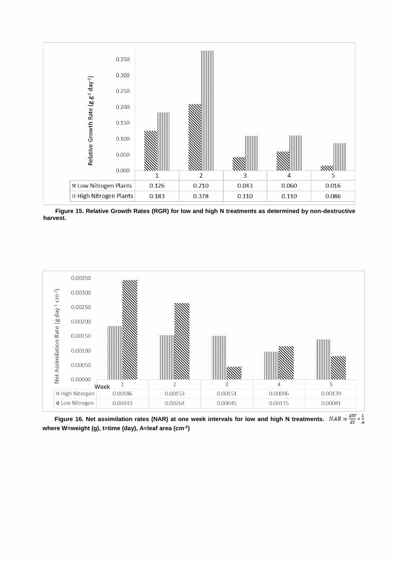
Week
Figure 16. Net assimilation rates (NAR) at one week intervals for low and high N treatments.
where W=weight (g), t=time (day), A=leaf area (cm-2)
Figure 15. Relative Growth Rates (RGR) for low and high N treatments as determined by non-destructive harvest.
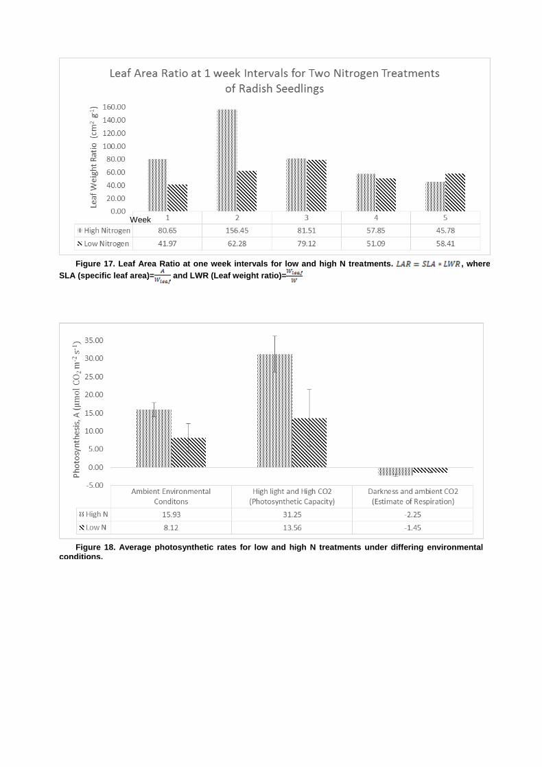
Figure 18. Average photosynthetic rates for low and high N treatments under differing environmental conditions.
Week
Figure 17. Leaf Area Ratio at one week intervals for low and high N treatments. , where
SLA (specific leaf area)= and LWR (Leaf weight ratio)=

Figure 20. Mean ratio of fluorescence during dark to light transition for low and high nitrogen treatments. N=12 for both averages, σlowN=0.090, σhighN=0.014.
Figure 19. Average leaf conductance for low and high N at differing environmental conditions.
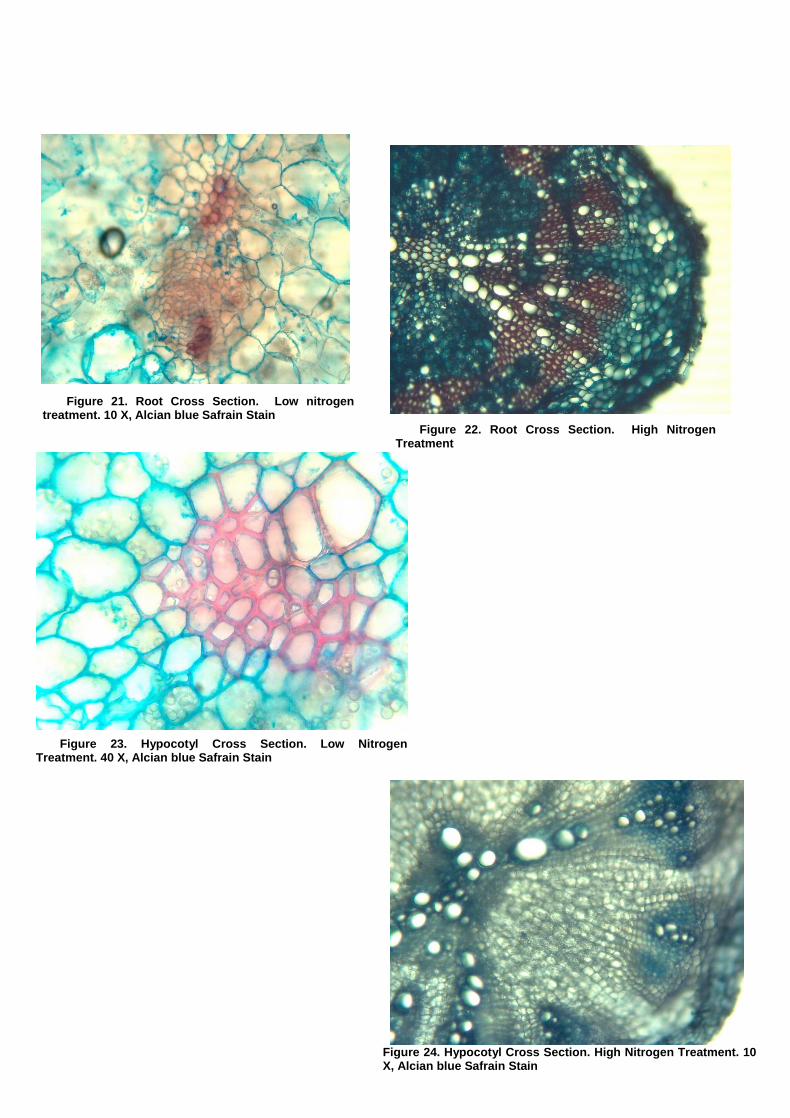
Figure 23. Hypocotyl Cross Section. Low Nitrogen Treatment. 40 X, Alcian blue Safrain Stain
Figure 24. Hypocotyl Cross Section. High Nitrogen Treatment. 10 X, Alcian blue Safrain Stain
Figure 22. Root Cross Section. High Nitrogen Treatment
Figure 21. Root Cross Section. Low nitrogen treatment. 10 X, Alcian blue Safrain Stain

Figure 25. Hypocotyl Cross Section. High Nitrogen Treatment. 10 X,
Iodine Stain
Figure 27. Stem Cross Section. High Nitrogen Treatment. 10 X
Figure 26. Hypocotyl Cross Section. Low Nitrogen Treatment. 10 X,
Iodine Stain
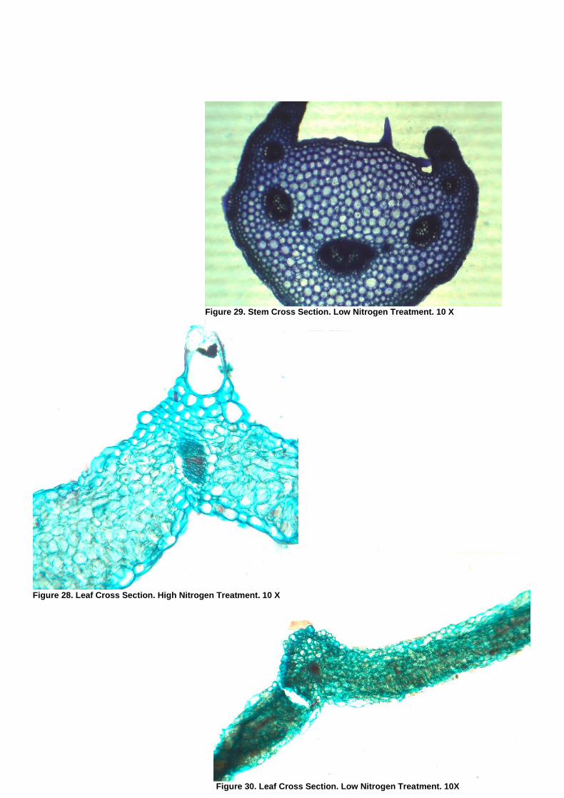
Figure 30. Leaf Cross Section. Low Nitrogen Treatment. 10X
Figure 28. Leaf Cross Section. High Nitrogen Treatment. 10 X
Figure 29. Stem Cross Section. Low Nitrogen Treatment. 10 X
Michael Dirks & Mark Weir
9 June 2013
Isolation and Identification of Putative Plant Growth Promoting Bacterial
Isolates Containing the acdS (ACC Deaminase) Gene
Introduction
The last 40 years have seen a dramatic increase in the scientific research surrounding soil ecology dynamics and the extensive bi-directional relationship between plants and soil microbes.1,2 Additionally, increased interest during the past decade in bacterial alternatives to conventional agricultural crop growth promotion have created an expanding body of research surrounding soil science and phenotypic microbial identification. One class of soil microorganisms which have received substantial inquiry are the purported Plant Growth Promoting Rhizobacteria (PGPR). These free living bacteria have been shown to increase plant growth by a number of mechanisms including, antibiotic/antifungal production, chelation/solubilization of nutrients such as iron and phosphorus, and synthesis/degradation of phytohormones. One of the more extensively studied promotion activities is the reduction - via catabolism - of the cyclic alpha amino acid, 1-aminocyclopropane-1-carboxylic acid (ACC) to ammonia and α-ketobutyrate (Figure 1). Under normal metabolism, plants convert stores of ACC to the phytohormone ethylene by way of the ACC oxidase enzyme. Ethylene in turn is tied to a host of transcription/translation regulatory mechanisms and phytohormone cascades/gradients.4 The storage of ethylene signalling capacity, in the form of ACC, allows plants to transport and regulate intercellular communication in a more manageable form than gaseous ethylene ( HYPERLINK \l "Van12" 6 ). Lowering ACC concentration has been shown to directly affect plant ethylene stress response and consequently developmental growth patterning7). Plants having a mutualistic or non-antagonistic relationship with PGPRs able to metabolise ACC – thus diminishing the intra/inter cellular levels of ACC and ultimately ethylene - develop faster, assimilate greater carbon dioxide through photosynthesis and survive stress conditions better than plants which lack associations with ACC deaminase possessing microbes ( HYPERLINK \l "Ono09" 8 ),9), ( HYPERLINK \l "Ran12" 10 ), 11), ( HYPERLINK \l "Gar" 12 ).
The conversion of ACC to ammonia and α-ketobutyrate by bacteria is dependent on the presence of ACC deaminase [EC 4.4.1.14]13). The ACC deaminase gene (acdS) is unique in that no plants have been shown to possess active copies of the resulting enzyme, restricting the non-hormonal degradation pathway in plants to bacterial associations. So significant is the effect of ACC deaminase activity that various groups have transgenetically modified bacteria and crops to express the gene, increasing yields ( HYPERLINK \l "Hol03" 14 ),15). With public opinion shifting to food lower in fertilizer and pesticide treatments, a search has been underway to rapidly identify and quantify bacterial strains which can actively metabolize ACC, resulting in increased plant growth.
Spanning the last 30 years, primary identification methods have involved the use of selective growth media. The development of consecutive dilutions, through increasingly selective media, concluded by a media containing only ACC as the source of nitrogen, has proven successful in selecting for PGPR ( HYPERLINK \l "Pen03" 16 ). Once isolated, putative PGPR must be identified for the presence of acdS. Determining the specific genes present and the microbial community of a site before the advent of Polymerase Chain Reaction (PCR) coupled to aggregate soil sampling was a difficult prospect involving culturing of only portions of the biota. Exploitation of the genetic conservation present among species in the 16S ribosomal RNA (16S rRNA) of bacteria chromosomes has proven a powerful mechanism for wider classification of microbial soil communities17). By amplifying the acdS and 16S rRNA genes from selectively isolated colonies, it is possible to identify bacteria having a high potential for plant growth promotion. Further, comparison of the genes with national

databases, such as the National Centre for Biotechnology Information (NCBI), allow for the phylogenetic placement within the bacteria kingdom.
Presented here are a series of experiments using selective media and gene amplification techniques aimed at the isolation and identification of ACC deaminase possessing rhizobacteria from commercial plant growth promotion inoculates and garden soil from the Southern Oregon University community garden. It is hypothesized that a majority of the commercial products will contain PGPR expressing the enzyme ACC deaminase as this is a common trait among PGPR. Additionally, given the extensive genetic diversity seen in other studies, it is postulated that isolated PGPR will be composed of a variety of bacterial genera. While the acdS gene is expected to be highly conserved among the isolates, some variability is anticipated, a result of diverse plant-bacteria interactions directing microbial transcriptional activity. Further, recent studies have indicated that varying degrees of horizontal gene transfer are present among bacteria possessing acdS, potentially resulting in a high degree of variability in the collective microbial community, especially among the garden soil samples ( HYPERLINK \l "Hon05" 18 ).
Materials and Methods
Five duplicate 1.0 g samples were obtained from the SOU community garden (2 sites) and 3 commercial products, Dr. Earth, Plant Success, and Organica (samples identified in Table 3). A negative control was carried throughout the experiment to reduce false positives and indicate environmental contamination. The samples were placed into individual 125-Erlenmeyer flasks (20 in total) and incubated 24 hours at 200 rpm and at 30 oC in 50 mL of PAF media (formulation of media, Table 1). After incubation, a 1-mL aliquot from each of the samples was transferred to a clean flask with 50 mL of PAF media. The incubation and 1-mL transfer was repeated with transfer to a second selective media, DF salt medium (formulation of media, Table 2) containing (NH4)2SO4 as the sole nitrogen source. From this medium, after identical incubation as before, 1-mL was transferred to a DF salt medium containing ACC as the nitrogen source. At this point, surviving isolates should contain the acdS gene which is required for the breakdown of ACC to release nitrogen for growth. These colonies were then plated on DF salt plates (1.8% Bacto-Agar) and 30 μmol of ACC and allowed to grow for 24 hours (30 oC). DNA samples from plates displaying growth where extracted using a DNeasy Blood and Tissue kit (Qiagen, Germantown, MD, USA). PCR amplification of an approximately 785 BP coding section of the acdS gene was performed according to the Caballero-Mellado et al. protocol with the primers acdSF 5’-ACGCCGATCCARCCGCTM-3’ and acdSR 5’-TCCAGCGTGCCSTCGTC-3’19). A 0.8 µL aliquot of cleaned bacteria template was added to a 40 µL PCR reaction mixture consisting of 27.9 µL H2O, 1X PCR buffer, 1.5 mM MgCl2, 25 µM dNTPs, 1 unit Taq, and 5 pmol of each primer. The reaction was heated at 95 °C for 5 min followed by 30 cycles consisting of 95 °C (45 sec), 67°C (45 sec), and 72 °C (1 min) and a final extension at 72 °C for 5 min. The resulting oligonucleotides were cleaned using QIAquick PCR Purification Kit and QIAquick Nucleotide Removal Kit (Qiagen, Germantown, MD, USA). Agarose gel examination of the PCR product indicated failure to amplify the acdS gene using the protocol so 16S rRNA amplification was undertaken.
PCR amplification of an approximately 1,500 BP coding section of the bacterial 16 S rRNA gene was performed with primers 8F 5’- AGAGTTTGATCCTGGCTCAG-3’ and 1492r 5’- GGTTACCTTGTTACGACTT-3’. A 0.7 µL aliquot of bacterial template was added to a 30 µL PCR reaction mixture consisting of 1X PCR buffer, 2.0 mM MgCl2, 200 µM dNTPs, 1.5 units Taq, and 2.5 µM of each primer. The reaction was heated to 94 °C for 2 min followed by 29 cycles consisting of 94 °C (30 sec), 52 °C (1 min), and 72 °C (3 min) and a final extension at 72 °C for 10 min. Purified DNA was analyzed with a ABI 310 Sequencer following treatment via the BigDye 3.1 kit (Life Technologies, Grand Island, NY, USA) using the 1492r primer. Sequence data was processed with Finch TV version 1.4.0 and compared against the NCBI data base using the Basic Local Alignment Search Tool (BLAST).

Results
Of the eight simultaneous sample runs (and the 2 negative controls), both of the SOU garden soils (2 locations), the Organica (2 samples), and Plant Success (2 samples) commercial products displayed growth in the DF salts-ACC growth broth (Table 3). Neither the Dr. Earth product (2 samples) nor the two negative controls revealed activity on the selective media (Table 3). Transfer to selective media plates further confirmed these results. Amplification of the acdS gene using the Caballero-Mellado et al. protocol produced no useable PCR product, as evidenced by the absence of a band at 785 BP on a gel (Figure 2). PCR amplification of the 16S rRNA gene was successful on all positive ACC samples with the exception of 1A and 1B, as confirmed by the 1,500 BP band on a gel of those amplifications (Figure 3). Absence of the 16S rRNA amplification for 1A and 1B (SOU soil sample #1) was confirmed by a second gel lane run (right hand side of Figure 3). Sequencing of the 16S rRNA gene from the 1492r primer produced a variety of fragment sizes (Table 4), each with a significant number of unresolved nucleotides (not shown). BLAST of the sequence data (not shown) resulted in diverse species identification, even within samples and with fluctuating levels of query coverage and max identity (Table 4). Notable are the unresolvable species from two the Organic samples (3A, 4A) and one of the Plant Success samples (8A) representing 3 of the longest fragment sections.
Discussion
Isolation of potential plant growth promoting bacteria using the Penrose and Glick selective media technique was highly successful, both among commercial products and soil samples. The former is not overly surprising given the plant growth promotion claims made by these products and the high prevalence of ACC deaminase in PGPR. The growth on all ACC deaminase selective plates by microbes from the SOU garden was however surprising to these researchers. Four different isolates were identified from garden samples and although 1A and 1B returned negative PCR results for 16S rRNA amplification, the presence of extensive growth on each plate speak to the high potential of ACC deaminase activity. While initial attempts to study the acdS gene present in putative PGPR where unsuccessful, subsequent 16S rRNA amplification and BLAST alignments produced a wide variety of identifications.
The failure of the Caballero-Mellado et al. acdS protocol can be speculatively assigned to the low quantities of PCR reagents called for in the procedure. Another explanation is that the primers, which Caballero-Mellado et al. designed for amplification of the acdS gene among nitrogen fixing Burkholderia in the tomato rhizosphere, may be too specific to successfully anneal with variations in the acdS genes found among other PGPR. The use of multiple acdS primers by experimenters such as Duan have allowed for greater variability in the characterization of bacterial isolates and may prove to be a more appropriate approach for future amplification attempts.20
Of the 16S rRNA amplifications, samples 1C, 2B and 2C (all from the SOU garden) share a similar 16S rRNA gene with the Acinetobacter genus. Acinetobacter, a Gram-negative (low peptidoglycan containing) soil microbe, is often associated with the breakdown of aromatic compounds and generally good soil heath.21 Additionally, Acinetobacter have been shown to possess the acdS gene and be widely distributed, showing up around the world, including the rizosphere of plants in locations as far away as the cold deserts of the Himalayas ( HYPERLINK \l "Gul09" 22 ) . The presence of the three Acinetobacter strains at the SOU garden site (similar to Acinetobacter sp. SA1, sp. MF-1 and baumannii strain NBRAJG79) point to a possible connection between the soil type and the microbial community it supports. Additionally, one of the two identifiable Organica isolates was of the Acinetobacter genus (sharing slight similar to species lwoffii strain Pt404), indicating that Acinetobacter verities may make good commercial products. Although not completed as part of this research, identifying conservation among the various Acinetobacter 16S rRNA genes may provide valuable insight into how closely related these three bacteria are and the level of PGP potential within the genus.
A review of the commercial products, Organica, Plant Success and Dr. Earth, produced an assortment of results. Significantly, the Dr. Earth product failed to produce colonies in either of the two flask containing ACC selective medium. Additionally, plating on ACC selective media with the Dr. Earth product (4 samples) produced similar negative results. While the product may contain PGPR, the absence of ACC deaminase activity, as indicated by the selective media technique, signifies low potentiality for the product to be a high plant growth promoter. Although not conducted as part of this research, sequencing of the microbes in the Dr. Earth product would provide insight into any potential value of the product. Of the other two products, Plant Success displayed results consist with expectations (bacterial species present) while Organica had successful growth yet contained a number of interesting and unidentifiable species. Bacillus and Pseudomonas present in the Plant Success product match with the expectations of the general PGPR expected, especially Bacillus which is widely owing to the its formation of endospores, making it easier to commercialize Notable is Plant Success marketing as a mycorrhizal product, not a bacterial product (no bacterial strains are listed on the packaging). It is not surprising that a mycorrhizal product would contain PGPR since these often work in concert to promote growth in plants. The presence of Eubacterium (similar to sp. 11-12) in the Oragainc product is not overly surprising given that such bacteria have been characterized as PGP and found in anthrosols (soil farmed extensively for centuries) by researchers such as O’Neill et al.23 The commercialization of microbes from such areas is logical in light of the use by farmers of such soil based on the success of multi-generational harvest.
Although the acdS gene was not specifically identified in the samples, the absence of nitrogen fixing bacterial species (Azotobacteraceae, Rhizobia, Frankia, ect.) across all samples supports the conclusion that the isolates did contain the ACC deaminase gene. Further study, using a variety of acdS primers should lead to conclusive support of the gene and will be the focus of ongoing research.
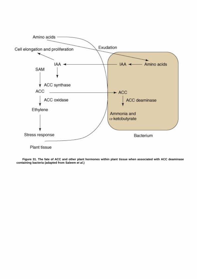
Figure 31. The fate of ACC and other plant hormones within plant tissue when associated with ACC deaminase containing bacteria (adapted from Saleem et al.)

Table 21. PAF medium formulation, dissolved in 1 L of H2O and sterilized
Media Component Amount
Casein 10.060 g
Peptone 10.001 g
MgSO4 1.512 g
K2PO4 1.580 g
Glygeain 10.0 mL
Table 22. DF Salts medium formulation, dissolved in 1 L of H2O and sterilized
Media Component Amount (g)
H3BO3 0.0165
MnSO4H2O 0.0114
ZnSO47H2O 0.1253
CuSO45H2O 0.0783
MoO3 0.0105
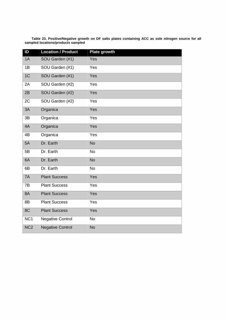
Table 23. Positive/Negative growth on DF salts plates containing ACC as sole nitrogen source for all sampled locations/products sampled
ID Location / Product Plate growth
1A SOU Garden (#1) Yes
1B SOU Garden (#1) Yes
1C SOU Garden (#1) Yes
2A SOU Garden (#2) Yes
2B SOU Garden (#2) Yes
2C SOU Garden (#2) Yes
3A Organica Yes
3B Organica Yes
4A Organica Yes
4B Organica Yes
5A Dr. Earth No
5B Dr. Earth No
6A Dr. Earth No
6B Dr. Earth No
7A Plant Success Yes
7B Plant Success Yes
8A Plant Success Yes
8B Plant Success Yes
8C Plant Success Yes
NC1 Negative Control No
NC2 Negative Control No

Figure 1. PCR products of acdS gene primers (Caballero et al. primers-protocol), expected
fragment size 785 BP, 1% agarose gel, SS (size standards), NC (negative control)
1B 2A 2
B 7A
8A SS
4A NC
NC 3B 1
A 1C 3
A 7B 8
C 4B 8
B

1A 1B 1
C 2A 2
B 2C 3A 3
B 4
B NC
7A 7B
8A 8B 8
C
SS
4A 1
A 1B 1C
Figure 2. PCR products of 16s rRNA gene (8F and 1492r primers, Oline protocol), expected
fragment size 1,500 BP, 1% agarose gel, SS (size standards), NC (negative control).
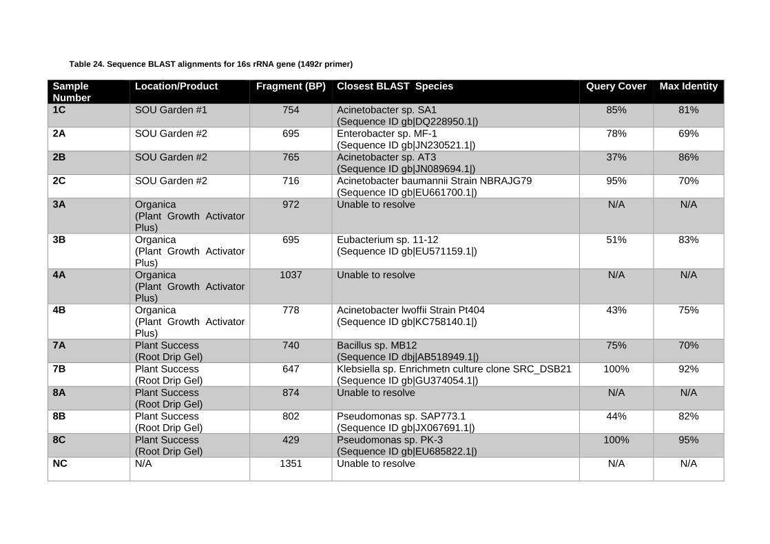
Table 24. Sequence BLAST alignments for 16s rRNA gene (1492r primer)
Sample Number
Location/Product Fragment (BP) Closest BLAST Species Query Cover Max Identity
1C
SOU Garden #1
754
Acinetobacter sp. SA1 (Sequence ID gb|DQ228950.1|)
85%
81%
2A
SOU Garden #2
695
Enterobacter sp. MF-1 (Sequence ID gb|JN230521.1|)
78%
69%
2B
SOU Garden #2
765
Acinetobacter sp. AT3 (Sequence ID gb|JN089694.1|)
37%
86%
2C
SOU Garden #2
716
Acinetobacter baumannii Strain NBRAJG79 (Sequence ID gb|EU661700.1|)
95%
70%
3A
Organica (Plant Growth Activator Plus)
972
Unable to resolve
N/A
N/A
3B
Organica (Plant Growth Activator Plus)
695
Eubacterium sp. 11-12 (Sequence ID gb|EU571159.1|)
51%
83%
4A
Organica (Plant Growth Activator Plus)
1037
Unable to resolve
N/A
N/A
4B
Organica (Plant Growth Activator Plus)
778
Acinetobacter lwoffii Strain Pt404 (Sequence ID gb|KC758140.1|)
43%
75%
7A
Plant Success (Root Drip Gel)
740
Bacillus sp. MB12 (Sequence ID dbj|AB518949.1|)
75%
70%
7B
Plant Success (Root Drip Gel)
647
Klebsiella sp. Enrichmetn culture clone SRC_DSB21 (Sequence ID gb|GU374054.1|)
100%
92%
8A
Plant Success (Root Drip Gel)
874
Unable to resolve
N/A
N/A
8B
Plant Success (Root Drip Gel)
802
Pseudomonas sp. SAP773.1 (Sequence ID gb|JX067691.1|)
44%
82%
8C
Plant Success (Root Drip Gel)
429
Pseudomonas sp. PK-3 (Sequence ID gb|EU685822.1|)
100%
95%
NC
N/A
1351
Unable to resolve
N/A
N/A
Works Cited
1. Ogram, A. Soil molecular microbial ecology at age 20: methodological challenges for the
future. Soil Biology & Boiochemistry 2000, 32, 1499-1504.
2. Haichar, e. Z.; Marol , C.; Berge, O.; Rangel-Castro, J. I.; Prosser, J. I.; Balesdent, J.;
Heulin, T.; Achouak, W. Plant host habitat and root exudates shape soil bacterial commuity
structure. The ISME Journal 2008, 2, 1221-1230.
3. Gupta, V. V. S. R. Benefical microorganisms for sustainable agriculture. Microbiology
Australia 2012, 113-115.
4. Burdman, S.; Jurkevitch, E.; Okon, Y. Recent advance in the use of plant growth promoting
rhizobacteria (PRPR) in agriculture. In Microbial Interaction In Agriculture Foresty; Subba
Rao, N. S., Dommergues, Y. R., Eds.; Science Publishers, Inc.: Plymouth, UK, 2000; Vol. II,
pp 229-250.
5. Saleem, M.; Arshad, M.; Hussain, S.; Bhatti, A. S. Perspective of plant growth promoting
rhizobacteria (PGPR) contianing ACC deaminase in stress agriculture. J. Ind. Microbiol.
Biotechnol. 2007, 34, 635-648.
6. Van der Ent, S.; Pieterse, C. M. J. The Plant Hormone Ethylene. In Annual Plant Reviews,
1st ed.; McManus, T., Ed.; Plackwell Publishing LTD, 2012; Vol. 44, pp 343-377.
7. Glick, B. R. Modulation of plant ethylene levels by the bacterial enzyme ACC deaminase.
FEMS Microbiology Letters 2005, 251, 1-7.
8. Onofre-Lemus, J.; Hernandez-Lucus, I.; Girard, L.; Caballero-Mellado, J. ACC (1-
Aminocyclopropane-1-Carboxylate) Deaminase Activity, a Widespread Trait in Burkholderia
Species, and Its Growth-promoting Effect on Tomato Plants. Appl. Environ. Microbiol. 2009,
75 (20), 6581-6590.
9. Sziderics, A. H.; Rasche, F.; Trognitz, F.; Sessitsch, A.; Wilhelm, E. Bacterial endophytes
contributed to abiotic stress adaptation in pepper plants (Capsicum annuum L.). Can. J.
Microbiol. 2007, 53, 1195-1202.
10. Rani, M. U.; Reddy, G.; Reddy , A. Screening of rhizobacteria containg plant growth
promoting (PGPR) traits in rhizosphere soils and their role in enhancing growth of pigeon
pea. Afr. J. Biotechnol. 2012, 11 (32), 8085-8091.
11. Kang, S. H.; Cho, H.-S.; Cheong, H.; Ryu, C.-m.; Kim, J. F.; Park, S.-h. Two Bacterial
Entophytes Elicting Both Plant Growth Promtoing and Plant Defense on Pepper (capsicum
annuum L). J. Microbiol. Biotechonl. 2007, 17 (1), 96-103.
12. Garcia-Gutierrez, L.; Romero, D.; Zeriouh, H.; Cazorla , F. M.; Tores, J. A.; de Vicente, A.;
Perez-garcia, A. Isolation and selection of plant growth-promoting rhizobacteria as inducers
of systemic resistance in melon. Plant Soil 2012, 385, 201-212.
13. Honma, M.; Simomura, T. Metabolism of 1-Aminocyclopropane-1-carboxylic acid. Agric.
Biol. Chem. 1978, 42 (10), 1825-1831.
14. Holguin, G.; Glick, B. R. Transformation of Azospirillum brasilense Cd with an ACC
Deaminase Gene from Enterobacter cloacae UW4 Fused to the Tetr Gene Promoter
Improves iIts Fitness and Plant Growth Promoting Abliltiy. Microb. Ecol. 2003, 46, 122-133.
15. Klee, J.; Kishore, G. M. CONTROL OF FRUIT RIPENING AND SENESCENCE IN PLANTS.
5,702,933, Dec 30, 1997.
16. Penrose, D. M.; Glick, B. R. Methods for isolating and characterizing ACC deaminase-
contianing plant growth-promoting rhizobactria. Physiol. Plant. 2003, 118, 10-15.
17. Woese, C. R. Phylogenetic structure of the prokaryotic domain: The primary kingdoms.
PNAS 1977, 11, 5088-5090.
18. Hontzeas, N.; Richarson, A. O.; Belimov, A.; Safronova, V.; Abu-Omar, M. M.; Glick, B. R.
Evidence for Horizontal Transfer of 1-Aminocyclopropane-1-carboxylate Deaminase Genes.
Appl. Environ. Microbiol. 2005, 71 (11), 7556-7558.
19. Caballero-Mellado, J.; Onofre-Lemus, J.; Estrada-de los Santos, P.; Martinez-Aguilar, L. The
Tomato Rhizosphere, and Environment Rich in Nitrogen-fixing Burkholderia species aiwth
Capabilites of Interest for Agricuture and Bioremediation. Appl. Environ. Microbiol 2007, 73
(16), 5308-5319.
20. Duan, J. 1-Aminocyclopropane-1-carboxylate (ACC) deminase genes in Rhizobia: Isolation
and characterization. Masters Thesis - University of Waterloo, Waterloo, Ontario, Canada,
2007; pp 1-108.
21. Williams, P. A.; Ray, C. M. Catabolism of Aromatic Compunds by Acinetobacter. In
Acinetobacter Molecualr Biology, 1st ed.;, 2008; pp 99-117.
22. Gulati, A.; Vyas, P.; Rahi, P.; Kasansa, R. C. Plant growth-promoting and rhizosphere-
compentent Acinetobacter rhizosphaera strain BIHB 723 fromt he cold deserts of the
Himalayas. Current microbiology 2009, 58 (4), 371-377.
23. O'neill, B.; Grossman, J.; Tsai, M. T.; Goes, J. E.; Lehmann, J. Bacterial community
compostion in Brazilian Anthrosols and adjacent soils characterized using culturing and
molecuar identification. Microb. Ecol. 2009, 58 (1), 23-25.

Computer Skills
Listed below are computer applications which Mark Weir has demonstrated proficiency in.
Molecular Modeling
Avogadro – Advanced molecule editor and visualizer - Version 1.1.0
ACD/ChemSketch – Chemical drawing program for organics, organometallics, polymers and Markush structures – Version 12.01
Accelrys/Symyx Draw – Chemical drawing program – Version 4.0
Cn3D – 3-D visualization tool for NCBI enzyme structure database – Version 4.3
Spartan – molecular modeling and computational chemistry application - Version 4.1.2
Spectroscopic Analysis
MestReNova - Nuclear Magnetic Resonance and LC/GC/MS data processing - Version 6.2.0-7238
Agilent Technologies Chemstation - GC/MS data acquisition, data processing, and reporting – Versions E.02.01.1177 and A.10.01(1635)
Programing and Mathematics
MATLAB – Matrix manipulation and plotting programming language – Version R2013b (8.2.0.701)
SCILAB – Open source numerical computation and orientation programing langue – Version 5.4.0
Mathcad – Computer algebra and SI unit calculation and verification workspace - Version 15.0 (MC15_M010_20110622)
Spreadsheets and Word Processing
Microsoft Office – Word, Excel and PowerPoint – Versions 1997, 2010 and 2013
Genetics
BioEdit – DNA sequence alignment and analysis toolpack – Version 7.2.5
FinchTV – DNA sequence analysis tool – Version 1.4.0
MEGA 6 – DNA sequence, alignment and phylogenetic tree analysis tool – Version 6.06

Research
Spanning nearly 3 years, the capstone research presented on the following pages is the culmination of an extensive and multidisciplinary study into Plant Growth Promoting Rhizobacteria (PGPR) with specific emphasis on endophytes possessing the 1-aminocyclopropane-1-carboxylic acid (ACC) deaminase enzyme. A hydrolase, ACC deaminase is active in select plant associated microbes and functions by degrading the ethylene precursor, 1-aminocyclopropane-1-carboxylic acid (a central phytohormone), to the hormonally inactive compounds, ammonia and α-ketobutyrate. In turn, this stimulates vegetative development by reducing the presence of ethylene in plant tissue, thus altering plant growth patterning, especially under drought, salt or pathogen stress.
An experimental framework is described for identifying putative beneficial bacteria at agricultural sites in Kalmatha Falls, Oregon. Differential phylogenic and ACC deaminase activity among PGPR was studied as it related to soil salinities at five sites with purported characteristics ranging from alkaline or neutral. Aqueous soluble salts and pH were measured using EPA method 9045D and the cations: lithium, aluminum, calcium, magnesium, potassium and sodium, were quantified using Inductivity Coupled Plasma – Optical Emission Spectroscopy. Separation and isolation of bacteria exhibiting ACC deaminase activity was accomplished using the Penrose & Glick method, a technique utilizing minimal media with ACC as the sole nitrogen source. Segregated ACC deaminase competent bacteria were supplied known quantities of ACC and enzymatic velocities measured by quantifying the metabolism rate of the substrate. A review of current approaches for derivatizing small amino acids such as ACC was conducted, including contrasting and assessing methods by honing a methanol:acetic acid (99:1) extraction solvent and using a silylation reagent. Employment of optimized methodologies and the derivatization agent, N-methyl-N-(tert-butyldimethylsily)tri-fluoroacetamide (MTBSTFA) allowed for the picomole determination of ACC and the potential for increased clarity in describing ACC deaminase kinetics among isolates. Quantification of the derivatized ACC was accomplished by comparison against an internal standard (5α-cholestane) after separation on a (5%-phenyl)-methylpolysiloxane gas chromatography column and detection using a quadrupole electron ionization mass spectrometer.
Phylogenetic analysis consisted of comparison of sequence data from PCR amplification of the 16S rRNA gene against the NCBI database using BLAST. Amplification of the acdS and nif genes with various primers produced for further classification of PGPR including correlation with parent soil profile. In total, 20 isolated γ-proteobacteria were identified with ACC Deaminase enzyme velocity established for five isolates. The five thoroughly studied bacteria included Pantoea, Azotobacter vinelandii, Klebsiella oxytoca, Pseudomonas fluorescnes and Buttiauxella agrestis. Enzymatic activity, measured as µmol of ACC catabolized per hour per total mg of protein was 3.7, 1.6±0.6 (n=4), 7.2±0.3 (n=4), 10.8±1.1 (n=4) and 5.1±0.2 (n=4) respectively. Total protein was measured by Bradford Assay at 595 nm on lysed cell extract. K. oxytoca, P. fluorescnes and B. agrestis were isolated from sites with elevated levels of soluble ions, +5.49 times more Na compared to neutral sties. The Pantoea isolate was from an elevated salinity soil, 2.46 times greater Na than the neutral site.
A bioassay using Raphanus sativus (Radish) and the K. oxytoca bacteria was conducted to confirm plant growth promotion capability. The hydroponic assay measured growth differences between low and high nitrogen treatments over a 5 week period. Low nitrogen treatments inoculated with the PGPR showed a 117% increase in growth over the low nitrogen control (average leaf area of 33.3 cm-2 vs 15.3 cm-2). Although the PGPR treatment did not show leaf areas as large as a high nitrogen treatment (76.6 cm-2 vs 33.3 cm-2), photosynthesis, stomatal conductance and chlorophyll fluorescence displayed increased growth metrics vs the low

nitrogen control (11.16 µmol CO2 m-2 s-1, 0.28 mol H2O m-2 s-1 and 0.7101 Fv/Fo respectively) indicating growth promotion.

Cooperative Learning
Listed below are various events and experiences where Mark Weir’s chemical knowledge has been applied in the community.
Ashland High School Chemistry Mentor – Spring 2014 Conducted weekly workshops for high school chemistry students under the direction of
Mr. Jim Lebo. Assisted students in labs presenting the creation of aromatic compounds. Ashland High School Biology Mentor – Winter 2013 Conducted weekly workshops for high school biology students under the direction of Mr.
Jim Hartman. Presented lectures on biochemistry and metabolism. Rogue Valley Salmon Festival – 2013 Developed and hosted the City of Ashland Conservation Commission informational
booth at the Rogue Valley Salmon Festival, including car wash capture demonstration. Rogue Valley Earth Day – 2012, 2013 Developed and hosted the City of Ashland Conservation Commission informational
booth at the Rogue Valley Earth day, including children’s compost games, household chemical use and car wash capture demonstration.
SOU Organic Chemistry Mentor – Fall 2012 Conducted weekly workshops for first term organic chemistry students alongside
Michael Dirks. SOU Biology Teaching Assistant – Summer 2012 Taught weekly lab sections and 3 lectures for Biology 102 under the direction of Dr. John
Sollinger. Green Drinks – Ashland 2011, 2012 Presented twice at green drinks, talks included: Gray Water: Safety, reuse and
conservation in Ashland OR & The StrawJet System: Application of appropriate technology in Malawi to Reduce Emissions from Deforestation and forest Degradation (REDD)
City of Ashland Conservation Commission – 2011 to 2014 (Chair, 2012-2013) Collaborated with city officials and citizen action groups to organize gray water reuse
symposium (SOU, 2012), storm water runoff analysis and plastic bag bans.

Honors and Awards
Following are awards and appointments earned by Mark Weir between 2011 and 2014.
Outstanding Analytical Chemist –Southern Oregon University – 2014
Elected Chair – City of Ashland Conservation Commission – 2013
Elected Sectary – Board of Directors – Habitat for Humanity Rogue Valley - 2013
Distinguished Presenter – Ashland Rotary – 2011
1 Pollan, M. 2002. This Steer’s life. The New York Times Magazine, March 31: pg 44
2 Siscovick, D. S; Raghunathan, T. E. Dietary Intake and Cell Membrane Levels of Long-Chain
n-3 Polyunsaturated Fatty Acids and the Risk of Primary Cardiac Arrest. JAMA 1995, 274(17),
1363-1367.
3 Lopez-Bote, C. J.; R.Sanz Arias, A.I;. Rey, A;. Castano, B.; Isabel, J;. Effect of free-range
feeding on omega-3 fatty acids and alpha-tocopherol content and oxidative stability of eggs.
Animal Feed Science and Technology 1998, 72, 33-40.
4 Ip, C; Scimeca J.A. Conjugated linoleic acid. A powerful anti-carcinogen from animal fat
sources. Cancer 1994, 74, 1050-1054.
5 Daley, C. A.; Abbott, A; Doyle, P. S.; Nader, G. A.; Larson, S. A review of fatty acid profiles
and antioxidant content in grass-fed and grain-fed beef. Nutrition Journal 2010, 9, 1-12.
6 Adam, O;, Beringer C; Kless T; Lemmen C; Adam A; Wiseman M; Adam P; Klimmek R;
Forth W. Anti-inflammatory effects of a low arachidonic acid diet and fish oil in patients with
rheumatoid arthritis. Rheumatol Int. 2003, 3, 27-36.
7 Turpeinen, A.M.; Mautanen, M.; Aro, A.; Salminen, I.; Basu, S.; Palmquist, D.L. Bioconversion
of vaccenic acid to conjugated linoleic acid in humans. American Journal of Clinical Nutrition
2002, 75,504-10.
8 Alves, S.P.; Marcellno, C.; Portugal, P. V.; Bessa, J. B. Short Communication: The Nature of
Heptadecenoic Acid in Ruminant Fats. J. Dairy Sci. 2005, 89, 170-173
9 Alonson, L.; Fontecha, J.; Lozada, L; Fraga, M.J.; Juarez, M. Fatty acid composition of caprine
milk: major, brached-chaing and trans fatty acids. J. Dairy Sci. 1999, 82, 878-884.
10 Abbey. M.; Nestel, P. J. Plasma cholesteryl ester transfer protein activity is increased
when trans-elaidic acid is substituted for cis-oleic acid in the diet. Atherosclerosis, 1994, 106,
99–107.
11 Rausch, C.; Weber, T.; Kohlbacher, O.; Wohlleben, W.; Huson, D. Specificity prediction of
adenylation domains in nonribosomal peptide synthetases (NRPS) using transductive support
vector machines (TSVMs). Nucleic Acids Res.2005, 33, 5799-5808.
12 Kohen, R.; Yamamoto, Y.; Ames, B. N. Antioxidant activity of carnosine, homocarnosine, and anserine present in muscle and brain. Proc. Natl. Acad. Sci. USA 1988, 85, 3175-3179.

13 Nakajima, T.; Wolfgram, F.; Clark, W. G. THE ISOLACTION OF HOMOANSERINE FROM BOVINE BRAIN. J. Neurochem. 1967, 14, 1107-1112.
14 Edmand, P.; Hogfeldt, E.; Sillen, L. G.; Kinell, P. Method for determination of the amino acid
sequence of peptides. Acta Chem. Scand. 1950, 4, 283-293. 15 Pisano, J. J.; Bronzert, T. J. Advances in the gas chromatographic analysis of amino acid
pheny- and methythiohydantions. Anal. Biochem. 1972, 45, 43-59.
16 Gottlieb, H. E.; Kotlyar, V.; Nudelman, A. NMR Chemical shifts of Common Laboratory
Solvents as trace impurities. J. Org. Chem. 1997, 62, 7512-7515.
17 Quirt, A. R.; Lyerla, J. R., Peat, I. R.; Cohen, J. S., Reynolds, W. F., Freedman, M. H. Carbon-13 Nuclear Magnetic Resonance Titration Shifts in Amino Acids. J. AM. Chem. Soc. 1974, 96, 570-574.
18 Schwarzinger, S.; Kroon, G. J. A.; Foss, T. R.; Wright, P. E.; Dyson, H. J. Random coil
chemical shifts in acidic 8M urea: implementation of random coil shift data in NMRView. J.
Biomol. NMR, 2000, 18, 43-48.
19 Bundi, A. and Wuthrich, K. 1H-NMR parameters of the Common Amino Acid Residues Measured in Aqueous Solutions of the Linear Tetrapeptides H-Gly-Gly-X-L-Ala-OH. Biopolymers, 1979, 18, 285-297.
20 Richarz, R. and Wuthrich, K. Carbon-13 NMR chemical Shifts of the Common Amino Acid Residues Measured in Aqueous Solutions of the Linear Tetrapeptides H-Gly-Gly-X-L-Ala-OH. Biopolymers, 1978, 17, 2133-2141.
21 Wuthrich, K. NMR in Biological Research: Pepdtides and Proteins. North Holland,
Amsterdam , 1976.