MARINE SCIENCE INSTITUTE

750 Channel View Drive • Port Aransas, Texas 78373-5015 ·Phone (361) 7~51~ (361) 749-6777

February 1, 2006 FEB 0 9 ?.GGo

Carla G. Guthrie Natural Resource Specialist Texas Water Development Board 1700 North Congress Ave. P.O. Box 13231 Austin, TX 78711-3231

RE: Submission of Final Report entitled, "Verification of Bay Productivity Measurement by Remote Sensors" Interagency Cooperative Contract Number: IA03-483-003

Dear Dr. Guthrie,

Enclosed please find copies of the referenced final report. As required, I have enclosed one electronic copy, one single-sided hard copy, and nine double-sided hard copies. This final report is a revised version of the draft report sent in July 2004. I have revised the report to include all suggestions made by the review team. As such, this report closes this study project.

I would like to thank you and the Board for your past and continued support of my research. I find this relationship very gratifying, and hope that you have gotten information that is directly applicable to your management needs.

If you need any further information, please call me at (361)749-6779, or FAX (361)749-6777, ore­mail paul@utmsi.utexas.edu.

Sincerely,

Paul Montagna, Ph.D. Research Professor

Russell et al. 1

1 2 Left running head: M. J. Russell et al.

3 Right running head: Estuarine Health and Function

4

5 Title: Effect of Freshwater Inflow on Estuarine Health and Function: Estimated by Whole

6 Ecosystem Metabolism

7

8 Names and address of authors:

9 Marc J. Russel11

10 Paul A. Montagna

11 Richard D. Kalke

12 University of Texas Marine Science Institute

13 750 Channel View Dr., Port Aransas, TX 78373

14

15

16

17 Submitted to: Estuaries

18 Draft date: June 2, 2004

19

20

21

22

23

24 1Corresponding author (361) 749-6817, marcr@utmsi.utexas.edu

Russell et al. 2

25 Abstract:

26 Freshwater inflow is necessary to maintain health and productivity in estuarine ecosystems.

27 There are no standard criteria to set inflow levels, however. Also, freshwater inflow rates are

28 changing due to changing land use patterns, water diversions for human consumption, and

29 climate effects. There is a need to be able to predict how changing hydrology might affect

30 estuary health. One indicator of estuarine health is ecosystem function of which whole

31 ecosystem metabolism is a major component. It was hypothesized that whole ecosystem

32 metabolism in shallow estuaries will depend on freshwater inflow. To test this hypothesis, whole

33 ecosystem metabolism was calculated in Lavaca Bay, Texas and its relationship to freshwater

34 inflow determined. We calculated a significant indirect relationship between whole ecosystem

35 metabolism and freshwater inflow near to the freshwater source in the upper bay, with more

36 negative whole ecosystem metabolism occurring after higher freshwater inflow events. No

3 7 significant relationship was found between whole ecosystem metabolism and freshwater inflow

38 in the lower bay. The relationship between freshwater inflow and net ecosystem metabolism

39 could be useful in total maximum daily load (TMDL) programs for dissolved oxygen

40 impairment. We conclude that fresh:Water loading i.e., the combination of water quality and

41 quantity, drives ecosystem function in shallow water estuaries. The location of freshwater inflow

42 sources within an estuary, however, is important in regulating this relationship.

43

44

45

46

47

Russell et al. 3

48 Introduction

49 Freshwater inflow is necessary to maintain both primary and secondary productivity in coastal

50 estuary ecosystems. Minimum freshwater inflow levels are required by many states to protect

51 estuarine health, but there is no standard approach or criterion to set inflow levels (Montagna et

52 al. 2002). Also, freshwater inflow rates are changing because of changes in land use, water

53 diversion for human consumption, and climate change effects. These anthropogenic changes

54 result in decreased freshwater inflow and changes in the capture and reduction of flood events.

55 There is a need to be able to predict how these anthropogenic changes in hydrology might affect

56 estuarine health. Estuarine health is the ecological integrity of an entire system. Ecological

57 integrity can be defined as a condition of ecosystems that is fully developed when the network of

58 biotic and abiotic components and processes is complete and functioning optimally (Campbell,

59 2000). A reliable and accurate indicator of estuarine health is ecosystem function.

60

61 An important component of ecosystem function is whole ecosystem metabolism. Whole

62 ecosystem metabolism is calculated by subtracting respiration from primary production for all

63 biological components contained in a defined body of water. A positive whole ecosystem

64 metabolism indicates that primary production exceeds respiration. A negative whole ecosystem

65 metabolism means that respiration exceeds primary production. In the aquatic environment,

66 whole ecosystem metabolism depends on a variety of physical and biological factors. Physical

67 factors that influence whole ecosystem metabolism include depth, surface wind speed,

68 freshwater inflow, turbidity, substrate type, salinity, temperature, flow rates, nutrient

69 concentrations, and tidal cycles. Biological factors that influence whole ecosystem metabolism

70 include chlorophyll-a, amount of live biomass in the water column and sediment, photosynthesis

Russell et al. 4

71 rates, and respiration rates. Changes in whole ecosystem metabolism may be driven by short

72 term events, seasonal, or annual cycles of environmental conditions. Freshwater inflow, by

73 delivering nutrients and organic matter from the watershed, may be the most important of these

7 4 environmental conditions by affecting the health, function, and productivity of estuarine

75 ecosystems.

76

77 Whole ecosystem metabolism is linked to dissolved oxygen dynamics through the processes of

78 photosynthesis and respiration. Dissolved oxygen concentrations must remain sufficiently high

79 to preserve ecosystem health. There are currently 4641 impaired water bodies in the United

80 States listed on the Environmental Protection Agency's 2002 303(d) list for organic

81 enrichment/low dissolved oxygen. Low dissolved oxygen ranks 5th on the top 100 impairments

82 list. Low dissolved oxygen is responsible for the approval of 94 7 total maximum daily load

83 (TMDL) programs, representing over 10% of the total number currently approved. One effect of

84 dissolved oxygen dynamics that has received recent interest is bottom water hypoxia events

85 during summer months. Causes of bottom water hypoxic conditions include water column

86 stratification, nutrient enrichment, and organic matter decomposition (Officer et al., 1984;

87 Pokryfki and Randall, 1987; Rabalais et al. 2001). The balance between water/sediment interface

88 photosynthesis and respiration can determine whether these waters become hypoxic or anoxic.

89 Large areas of shallow water estuaries can become hypoxic during summer months when high

90 levels of water column primary production, stratification, benthic respiration, and reduced

91 flushing by freshwater inflow reduce bottom water dissolved oxygen levels to dangerous levels

92 (<2.0 mg 0 2 1-1). Over one half of the estuaries in the Gulf of Mexico exhibit moderate to severe

93 dissolved oxygen depletion (hypoxia/anoxia), a key indicator of aquatic ecosystem health

Russell et al. 5

94 (Bricker et al. 1999). Hypoxia in Corpus Christi Bay was documented in the summer months of

95 1988 (Montagna and Kalke 1992) and has occurred every summer since (Montagna and

96 Morehead 2003). Organic matter and nutrients delivered by freshwater inflow not only effect

97 estuarine health but also estuarine function.

98

99 Ecosystem function in Texas shallow water estuaries may be altered by anthropogenic

100 modifications of Texas watersheds and the subsequent changes in freshwater inflow dynamics.

101 Restored inflow to Rincon Bayou Texas, after damming reduced freshwater inflow by 55%,

102 resulted in infauna abundance, biomass, and diversity increases (Montagna et al, 2002).

103 Increased freshwater inflow restored the ecosystem function of this salt marsh nursery habitat for

104 estuarine dependent, commercially important species such as the brown shrimp, Farfante

105 penaeus aztecus (Riera et al, 2000). Ecosystem function often translates into ecosystem

106 productivity.

107

108 Ecosystem productivity may be related to freshwater inflow by supplying nutrients and organic

109 matter from the watershed. Freshwater inflows to South Texas estuaries are limited ( ~0-800

110 million m3 y-1). An analysis of open water dissolved oxygen measurements to calculate

111 ecosystem metabolism over the past 20 years concluded that some Texas estuaries have low

112 amounts of gross primary productivity with only 200 g C m-2 y-1 (Ward, 2003). Low gross

113 primary production may be due to lack of freshwater inflow. Both organic matter and nutrients

114 can be used to fuel primary and secondary production in an estuary either directly by

115 incorporation into new biomass or indirectly by re-mineralization.

116

Russell et al. 6

117 Open water dissolved oxygen measurements have been used to estimate whole ecosystem

118 metabolism, providing spatially and temporally integrated estimates of metabolic processes since

119 Odum's seminal work in the 1950's (Odum 1956). Whole ecosystem metabolism is a

120 calculation of the change in dissolved oxygen concentration resulting from biological processes

121 in an aquatic ecosystem over a period of 24 hours. Atmospheric oxygen flux must be estimated

122 to separate physical and biological influences on dissolved oxygen concentration (Odum and

123 Wilson 1962). Atmospheric oxygen flux is influenced by a combination of dissolved oxygen

124 concentration gradients and near surface turbulence dynamics. The physical factors driving near

125 surface turbulence must therefore be accounted for during calculations of whole ecosystem

126 metabolism.

127

128 It was hypothesized that whole ecosystem metabolism in shallow estuaries will depend on

129 freshwater inflow. To test this hypothesis, whole ecosystem metabolism was calculated in

130 Lavaca Bay, Texas and its relationship to freshwater inflow determined. We calculated whole

131 ecosystem metabolism from continuous oxygen measurements and compared them to freshwater

132 inflow amounts.

133

134 Materials and Methods

135 A monitoring plan was designed to assess both the spatial and temporal variability in whole

136 ecosystem metabolism using dissolved oxygen concentrations in Lavaca Bay. Fifty-eight 24-

13 7 hour water quality monitoring samples, 20 water column nutrient samples, 43 water column

138 chlorophyll-a, and 50 sediment samples were taken over a two year period (2002-2003) (Table

139 la and lb). Six different Texas Commission of Environmental Quality (TCEQ) sites were

Russell et al. 7

140 sampled to provide spatial coverage (Table 2) (Fig. 1) (http://www.tceq.state.tx.us). Sites were

141 divided into upper bay (stations 1-3), and lower bay (stations 4-6) groups. The upper, lower bay

142 groups are subdivided by a constriction caused by the Highway 35 overpass (Fig. 1). Dissolved

143 oxygen and other water quality parameter measurements were taken every 15 minutes at mid-

144 depth using YSI series 6 multiparameter data sondes. Models 6920-S and 600XLM data sondes

145 with 610-DM and 650 MDS display loggers were used. The series 6 parameters have the

146 following accuracy and units: temperature(± 0.15°C), pH(± 0.2 units), dissolved oxygen (mg r1

147 ± 0.2), dissolved oxygen saturation(%± 2%), specific conductivity(± 0.5o/o of reading

148 depending on range), depth(± 0.2 m), and salinity(± 1% of reading or 0.1 ppt, whichever is

149 greater). Salinity is automatically corrected to 25°C.

150

151 The relatively high wind speeds that occur across the shallow water estuaries of Texas imply that

152 wind will dominate the physical control of atmospheric oxygen flux. Texas estuaries experience

153 sustained wind speeds commonly around 7-8 m s·1 (""13-18 mph), but can have daily variations

154 in wind speed from 1-10m s·1 (~2-23 mph) (Texas Coastal Ocean Observation Network data at

155 http://lighthouse.tamucc.edu/TCOON/HomePage). Estuaries in other regions of the U.S. tend to

156 have wind speeds in the range of0-6 m s·1 (""0-12 mph) with maximum atmospheric oxygen

157 exchanges measured at 8.6 m s·1 ("" 19 mph) (Kemp and Boynton 1980; Marino and Howarth

158 1993). Meteorological forcing dominates water exchange and circulation in South Texas

159 estuaries because of shallow water depths (medium depth ""2-4m), small tidal range (~0.25 m),

160 little freshwater inflow (~0-800 million m3 y"1), and long over-water fetches (Orlando et al.

161 1993). These characteristics when combined with ample sunlight, high temperatures, and

162 relatively steady South-east winds make South Texas estuarine ecosystems particularly amenable

Russell et al. 8

163 to open water methods of estimating whole ecosystem metabolism. Biological processes can still

164 dominate dissolved oxygen concentration changes in South Texas estuaries even with the

165 prevalence of high wind speeds. The physical features of South Texas estuaries, when combined

166 with the highly dynamic and large influence of wind speed on surface turbulence, require that

167 estimates of whole ecosystem metabolism in this region adjust for changes in atmospheric

168 oxygen flux because of changing wind speeds.

169

170 The wind dependent diffusion coefficients given by D 'A vanzo et al. (1996) were applied to

171 calculations of whole ecosystem metabolism in Lavaca Bay. D' Avanzo et al. 's diffusion

172 coefficients allowed for diffusion corrected calculations of dissolved oxygen concentration

173 change that could vary over short temporal scales (hourly). The major physical influence on

174 whole ecosystem metabolism calculations was thus removed by adjusting for atmospheric

175 oxygen flux generated during undersaturated or supersaturated dissolved oxygen concentration

176 conditions. Removal of the physical influences on dissolved oxygen concentration left just the

177 biologically driven changes in dissolved oxygen concentration.

178

179 Net ecosystem metabolism was calculated using open water diurnal methods. Dissolved oxygen

180 concentrations were taken every 15 minutes and converted to a rate of change in dissolved

181 oxygen concentration. These rates of change were then adjusted to control for diffusion of

182 oxygen between the water column and the atmosphere by using percent saturation of dissolved

183 oxygen in the water column and the wind dependent diffusion coefficient K (g 0 2 m-2 h-1) at Oo/o

184 saturation proposed by D'Avanzo et al. (1996) using the equation:

185

186

187

188

189

190

191

Russell et al. 9

Ric= R- ((1-((S1 + S2) I 200)) * K I 4); where

Ric = diffusion corrected oxygen concentration rate of change per 15 minutes,

R = observed oxygen concentration rate of change,

S1 and S2 =dissolved oxygen percent saturations at time one and two respectively,

K = diffusion coefficient at 0% dissolved oxygen saturation.

192 To calculate daily net ecosystem metabolism the 15-minute diffusion corrected rates of dissolved

193 oxygen change were then summed over a 24-hour period, starting and ending at SAM. Open

194 water dissolved oxygen methods similar to those used here have been used in a variety of

195 estuaries to calculate net ecosystem metabolism (Kemp et al 1992; D 'A vanzo et al. 1996; Borsuk

196 et al. 2001; Caffrey 2003).

197

198 Net ecosystem metabolism was regressed against freshwater inflow, salinity, water temperature,

199 water column depth, water column chlorophyll-a, water column nutrients, and sediment

200 characteristics. Freshwater inflow was calculated by summing all daily USGS gauged river flow

201 (millions of cubic feet day-1) into the bay during the ten days prior to sampling

202 (http:llwaterdata.usgs.govltxlnwislrt). A ten day period was assumed to be the time interval

203 needed to capture an estuary's response to relatively recent freshwater inflow. Salinity, water

204 temperature, and depth daily means were calculated from multiparameter sonde measurements.

205 Chlorophyll-a was sampled by modifying the TCEQ's Surface Water Quality Monitoring

206 Procedures Volume 1 (2003) (http:llwww.tnrcc.state.tx.usladmin/topdoclrg/4151415.html)

207 methods for collection of routine water chemistry samples. Two 1 0-ml sub-samples from a 1-L

208 van Doran bottle were collected and filtered on site. Chlorophyll-a concentration was

Russell et al. 10

209 determined using non acidification fluorometric techniques (W elschmeyer 1994 ). Water column

210 nutrient analyses for ammonium, phosphate, silicate, and nitrate plus nitrite were run on a Lachat

211 Quikchem 8000 using standard colormetric techniques (Parsons et al1984, Diamond 1994).

212

213 Sediment and macrobenthos were sampled by taking five 6. 7 em diameter cores per station.

214 Three cores were divided into 0-3 em and 3-10 em sections, and preserved in formalin until

215 macro benthic analysis. One core was divided into 0-3 em and 3-10 em sections for sediment

216 grain size analysis; all of the 0-3 em section and a vertical slice of the 3-10 em section were

217 collected in the field, but only 20 cm3 were used in analysis. Zero to 1 em and 2-3 em sections

218 from the final core were placed in sterile Petri dishes for total carbon, total nitrogen, and total

219 organic carbon analyses.

220

221 Results

222 Principle component analysis (PCA) of site specific environmental variables yielded two

223 relatively distinct groups of stations located in upper and lower Lavaca bay. Two groups of

224 stations; 1, 2, and 3 in upper Lavaca bay and station 4, 5, and 6 in lower Lavaca bay were

225 identified from salinity, temperature, and depth measurements taken during every 24-hour

226 dissolved oxygen deployment (Fig. 2a). Salinity and temperature had the highest loading values

227 with depth being similar to salinity (Fig. 2b ). Principle components 1 and 2 explained 56.3%

228 and 28.1 o/o respectively of the total variability. The station groups resulted from a gradient of

229 high salinity conditions at station 6 in the upper left to lower salinity conditions at station 1 in the

230 lower right (Fig. 2a). Temperature depended on time of year when samples were collected with

Russell et al. 11

231 lower temperatures corresponding to the lower left and higher temperatures in the upper right

232 (Fig. 2a).

233

234 Chlorophyll-a measurements resulted in similar station groups as the environmental condition

235 analysis (Fig. 3). Stations grouped together into three sets; 1 in upper bay, 3, 5, and 6 in lower

236 bay, and stations 2 and 4 made up a transitional group. Significant differences were seen

237 between station 1 and the group of stations 3, 5, and 6. Stations 2 and 4 grouped with both upper

238 and lower bay groups. The discrepancy between site 3 and 4 falling in an alternate group than

239 during the environmental condition analysis may be due to resuspension of benthic algae by

240 turbulence generated as water moves past an overpass located down estuary from station 3 and

241 up estuary of station 4. Chlorophyll-a did not have a significant relationship with net ecosystem

242 metabolism (linear regression, p = 0.5821) (Fig. 4).

243

244 Water column principle component nutrient analysis separated stations along a gradient from

245 upper to lower bay. The large change in nutrient concentrations during a large pulse of

246 freshwater inflow implies that the main driving force behind nutrient concentrations is freshwater

247 inflow (Fig. Sa). Upper bay stations encounter slightly higher concentrations of nutrients than

248 lower bay stations under lower freshwater inflow conditions (Fig. 5b ). Principle component 1

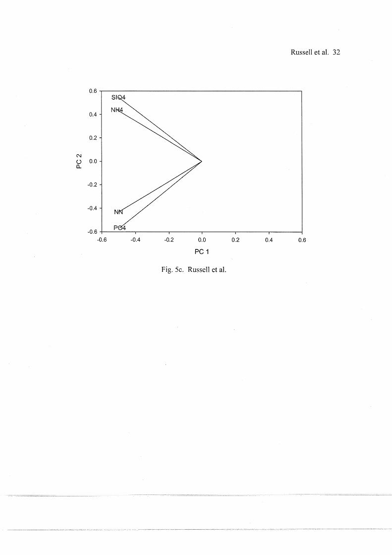
249 and 2 accounted for 83.3o/o and 7.9% respectively of the total variance (Fig. 5c).

250

251 Sediment characteristic PCA resulted in a separation between upper and lower bay stations (Fig.

252 6a). Principal component 1 and 2 accounted for 60% and 24% respectively of the total

253 variability (Fig. 6b ). Stations were vertically separated on PC 2 by a gradient of sandy sediment

Russell et al. 12

254 in upper bay to clay dominated sediments in lower bay. Lower bay stations also had more total

255 sediment nitrogen. Station 5 separated from the rest of the stations on PC 1 because of the large

256 quantities of total carbon, total organic carbon, and rubble measured there. The rest of the

257 stations were characterized by a larger percentage of silt and higher concentrations of total

258 nitrogen. No significant relationship was found between any sediment characteristic and net

25 9 ecosystem metabolism (linear regression, p = 0. 07 6-0.1 06).

260

261 Linear regression analysis comparing net ecosystem metabolism with freshwater inflow, salinity,

262 temperature, and depth resulted in only salinity (p < 0.001, R2 = 0.400) or freshwater inflow (p <

263 0.001, R2 0.374) being significant depending on which was entered into the model first.

264 Freshwater inflow will be used during the rest of the analysis instead of salinity since freshwater

265 inflow is more manageable by anthropogenic modification of watersheds than salinity.

266

267 Freshwater inflow correlated with net ecosystem metabolism in upper Lavaca bay (linear

268 regression p:S0.0001, R2 = 0.41) (Fig. 7). The largest net ecosystem metabolism residuals

269 occurred during the lowest levels of freshwater inflow into upper Lavaca bay. The most negative

270 net ecosystem metabolism values were calculated in upper Lavaca bay.

271

272 Lower Lavaca bay net ecosystem metabolism had an insignificant correlation with freshwater

273 inflow (linear regression p = 0.3497, R2 = 0.03) (Fig. 8). The largest response in net ecosystem

274 metabolism to freshwater inflow, however, was seen in lower Lavaca bay. The two large

27 5 positive values of net ecosystem metabolism in Lower Lavaca bay occurred at station 6 during

276 higher freshwater inflows. The lack of data during moderate freshwater inflows stems from the

Russell et al. 13

277 pulsing nature of precipitation events in Texas watersheds which are characterized by extended

278 periods of drought punctuated by flood events (Fig. 9).

279

280 Discussion

281 Freshwater inflow and salinity were determined to be the only factors to have a relationship with

282 net ecosystem metabolism in Lavaca Bay. Freshwater inflow and salinity, however, have a fairly

283 strong inverse relationship to each other (linear regression, p < 0.0001, R2 = 0.43) (Fig. 10).

284 Freshwater inflow is much more manageable than salinity because freshwater inflow is not as

285 affected by tidal and meteorological changes. The large variability in estuarine environmental

286 factors means that care must be taken to control for effects these factors may have on one's

287 response variable of interest, in this case net ecosystem metabolism. Separation of stations into

288 two groups located in upper and lower Lavaca Bay, even though no significant relationships

289 were found, allowed us to remove most of the effects on net ecosystem metabolism from station

290 differences in temperature, depth, chlorophyll-a, water column nutrients, and sediment

291 characteristics. The only other environmental factor that needed to be controlled for was

292 atmospheric water column oxygen diffusion.

293

294 The large influence that diffusion coefficients have on atmospheric water column oxygen

295 diffusion and the resulting net ecosystem metabolism values meant that we needed to choose an

296 appropriate diffusion equation for our specific ecosystem of study. Caffrey (2004) concluded

297 that 25o/o of daily measured oxygen concentration changes at 42 National Estuarine Research

298 Reserve (NERR) sites were due to atmospheric oxygen flux in water depths of approximately 1

299 meter. Estimates of diffusion coefficients and their relationship to wind speed have been

Russell et al. 14

300 calculated using a variety of methods. Odum and Hoskin (1958) used a method based entirely

301 on the rate of change of dissolved oxygen concentration in South Texas estuaries during night

302 time periods experiencing constant or near constant wind velocities. Their results suggest for

303 Texas shallow water estuaries the volumetric diffusion coefficient k (in mg 0 2 1"1 hf1 at 100%

304 saturation deficit) increases linearly from 0-3 as wind increases from 0-12 m s-1 (0-30 mph)

305 (Odum and Wilson 1962). Hartman and Hammond (1984) working in San Francisco Bay had

306 similar results and derived an area based wind-dependent diffusion coefficients K (in g 0 2 m-2 h-1

3 07 at 1 00% saturation deficit) that ranged from approx. 0-1.5 with wind speeds of 0-1 0 m s -1• Kemp

308 and Boynton (1980) assumed that atmospheric flux in relatively deeper systems varied as a

309 constant function of the oxygen gradient between surface water dissolved oxygen and

310 atmospheric gas with a diffusion coefficient that varied with both air and water turbulence. Their

311 estimates of gas transfer across the air-water interface from measurements using the floating

312 dome method (Copeland and Duffer 1964; Hal11970) yielded area based diffusion coefficients

313 of 0.9 to 9.7 g 0 2 m-2 h-1. Boynton et al (1978) also found a similar range ofK's (0.4-10.7 g 0 2

314 m-2 h-1) using a variety of methods. With more use of the floating dome method and

315 comparisons between different system types (i.e., estuaries, open ocean, and lakes) a more

316 complete picture of wind speed influence on atmospheric oxygen flux became available (Marino

317 and Howarth 1993). A general exponential relationship suggested by Smith (1985) was used to

318 model oxygen transfer velocity as a linear function of wind speed. Smith's log linear model

319 explained 55% of the atmospheric oxygen flux variability in a combined data set compiled from

320 a wide range of systems and measurement techniques (Marino and Howarth 1993). A recent

321 comparison of three wind-dependent diffusion coefficients with a constant coefficient of0.5 g 0 2

322 m-2 h-1 concluded that the constant coefficient was only similar to the wind-dependent

Russell et al. 15

323 coefficients at wind speeds from 0-5 m s-1 and greatly underestimated air-sea exchange at winds

324 greater than 8 m s-1 (Caffrey 2004) (Table 3). The three wind-dependent diffusion coefficient

325 equations are similar when plotted over wind speeds from 0-10 m s-1 (Fig. 11). D' Avanzo et al.

326 (1996), studying a shallow estuarine system in Waquoit Bay, Cape Cod, Massachusetts,

327 estimated relatively higher air-sea exchanges over the entire range of wind speeds than that

328 found for the wide range of systems used by Marino and Howarth (1993) which included deep

329 open ocean waters. A wind dependent diffusion coefficient similar to that proposed by D' Avanzo

330 et al. (1996) or Marino and Howarth (1993) is therefore preferable to assuming a constant

331 diffusion coefficient in systems encountering strong and highly variable wind speeds. We chose

3 3 2 to use D 'A vanzo et al. 's ( 1996) diffusion coefficients in our calculations of net ecosystem

333 metabolism's relationship to freshwater inflow because both of our estuarine systems have

334 shallow water depths.

335

336 Freshwater inflow alone is not driving whole ecosystem metabolism in estuaries, it is the organic

337 and inorganic loads contained in that inflow. We can define freshwater loading as the

338 combination of water quantity and quality. Freshwater inflow into an estuary contains organic

339 matter and nutrients from an estuary's corresponding watershed. Freshwater inflow rates can be

340 used as a proxy for freshwater loading from a specific watershed and will integrate watershed

341 level processes that effect both water quality and quantity. The relationship between freshwater

342 inflow and whole ecosystem metabolism was found to differ depending on location within a

343 shallow water estuary.

344

Russell et al. 16

345 In the upper bay, net ecosystem metabolism becomes more negative as freshwater loading

346 increases. A negative net metabolism value implies that an allochthonous source of organic

34 7 matter is being respired, and that daily respiration is higher than photosynthesis. This organic

348 matter sink may result in higher secondary production, but an extremely large negative net

349 ecosystem metabolism could lead to dissolved oxygen impairment as large amounts of oxygen

350 are converted to carbon dioxide during oxidation of organic matter. Upper Lavaca bay, being

351 located in close proximity to freshwater point sources, had the largest negative net ecosystem

352 metabolism response to increased freshwater inflow. Multiple freshwater point sources present

353 at Lavaca Bay (i.e. rivers and streams) may have led to the relatively larger variability in net

354 ecosystem metabolism during lower freshwater inflow periods. Shallow depths in the upper bay

355 may also have contributed to variability due to the effects of changing daily irradiance on benthic

356 primary production during low inflow periods when water clarity tends to increase. Upper bay

357 health and function, even with the increased variability at lower freshwater inflows, seem to be

358 primarily driven by levels of freshwater loading, but causality cannot be drawn from these results

359 due to use of correlation statistical analysis.

360

361 The lower bay, which likely receives less organic matter, has a more balanced to slightly positive

362 net ecosystem metabolism with increased freshwater loading. A balanced net ecosystem

363 metabolism implies that lower Lavaca bay doesn't act as a sink or source of organic matter. A

364 positive net metabolism value implies that autochthonous organic matter is being produced, and

365 the ecosystem is a net source of organic matter. Autochthonous matter production may be the

3 66 result of increased nutrient input from periods of increased freshwater flow. The two large

367 positive net ecosystem metabolism values during a period of high freshwater inflow occurred at

Russell et al. 17

368 station 6. Net ecosystem values closer to zero were found at station 4 during the same freshwater

369 inflow period. Upper bay conditions may push down into the lower bay where station 4 is

3 70 located during very high freshwater inflows. Station 4 may act as a transition between upper and

3 71 lower bay results during high freshwater inflows. If we separated the station 4 results from

3 72 stations 5 and 6 we could tentatively conclude that the lower bay has a large positive net

373 ecosystem response during high freshwater periods. The lack of replicate samples at station 5

374 and 6 during high freshwater inflows, however, means that further research will be needed before

375 valid conclusions about lower bay net ecosystem dynamics can be made. Autochthonous matter

376 production in lower Lavaca bay could, if severe, lead to eutrophic conditions and occurrences of

3 77 harmful algal blooms, but this is usually prevented in Lavaca bay by wind and tidal flushing, and

378 a well mixed water column. The deeper depths of the lower bay and the spatial separation from

3 79 freshwater inflow point sources implies that water column processes will dominate and tidal

3 80 forcing may be more important here than in the upper bay. The lack of significance in the

381 relationship between freshwater loading and whole ecosystem metabolism implies that other

3 82 factors are more important than freshwater loading this far away from freshwater inflow point

383 sources. Which factors are important, however, are still unknown.

384

385 These findings conclude that freshwater loading drives ecosystem function in shallow water

386 estuaries. The location within an estuary, however, is important in describing this relationship.

387 Whole ecosystem metabolism provides an indicator of ecosystem health and function but is also

388 a direct estimate of the biological processing of oxygen. Total maximum daily load programs for

389 dissolved oxygen impairment could use the techniques and relationships between freshwater

390 inflow and net ecosystem metabolism generated during this study and apply them to keep

Russell et al. 18

391 estuarine ecosystem metabolism in balance. Future research efforts include conducting broader

392 scale studies to quantify the temporal and spatial variability in net ecosystem metabolism's

393 relationship with freshwater inflow. The larger range of environmental conditions captured

394 during this future research will be used to produce a practical integrated watershed level

395 modeling tool for management of estuarine dissolved oxygen concentrations, health, and

396 function.

Russell et al. 19

Literature Cited

Borsuk, M .E., C. A. Stow, J. Luettich, H. W. Paerl, and J. L. Pinckney. 2001. Modelling

Oxygen Dynamics in an Intermittently Stratified Estuary: Estimation of Process Rates Using

Field Data. Estuarine, Coastal and Shelf Science 52: 33-49.

Boynton, W. R., Kemp, W. M., Osborne, C. G. and Kaumeyer, K. R. 1978. Metabolic

characteristics of the water column, benthos and integral community in the vicinity of Calvert

Cliffs, Chesapeake Bay. Contributed Report No. 2-72-02 (77), Maryland Power Plant Siting

Program, Annapolis, Maryland.

Bricker, S. B., C. G. Clement, D. E. Pirhalla, S. P. Orlando, and D. R. G. Farrow. 1999.

National estuarine eutrophication assessment: Effects of nutrient enrichment in the nation's

estuaries. NOAA, National Ocean Service.

Caffrey, J. M. 2003. Production, respiration, and net ecosystem metabolism in U.S. estuaries.

Environmental Monitoring and Assessment 81 : 207-219.

Caffrey, J. M. 2004. Factors controlling net ecosystem metabolism in U.S. estuaries. Estuaries

27 (1): 90-101.

Campbell, D. E. 2000. Using energy systems theory to define, measure, and interpret ecological

integrity and ecosystem health. In: Ecosystem Health 6(3): 181-204.

Russell et al. 20

Copeland, B. J. and W. R. Duffer. 1964. Use of a clear plastic dome to measure gaseous

diffusion rates in natural waters. Limnology and Oceanography 9: 494-499.

D' Avanzo, C., Kremer, J. N., and Wainright, S.C. 1996. Ecosystem production and respiration

in response to eutrophication in shallow temperate estuaries. Marine Ecology Progress

Series 141: 263-274.

Diamond, D. 1994. Lachat Instruments Inc., QuikChem method 31-115-01-1-A.

Hall, C. A. S. 1970. Migration and metabolism in a stream ecosystem. Ph.D. thesis. University

ofNorth Carolina, Chapel Hill.

Hartmon, B. and D. E. Hammond. 1984. Gas exchange rates across the sediment-water and air­

water interfaces in south San Fransisco Bay. Journal of Geophysical Research 89: 3593-

3603.

Kemp, W. M. and W. R. Boynton. 1980. Influence ofbiological and physical processes on

dissolved oxygen dynamics in an estuarine system: Implication for measurement of

community metabolism. Estuarine and Coastal Marine Science 11: 407-431.

Russell et al. 21

Kemp, W. M., P. A. Sampou, J. Tuttle, and W. R. Boynton. 1992. Seasonal Depletion of

Oxygen from Bottom Waters of Chesapeake Bay: Roles of Benthic and Planktonic

Respiration and Physical Exchange Processes. Marine Ecology Progress Series 85: 13 7-157.

Marino, R. and R. W. Howarth. 1993. Atmospheric oxygen exchange in the Hudson River:

dome measurements and comparison with other natural waters. Estuaries 16: 433-445.

Montagna, P. A. and Kalke, R. D. 1992. The effect of freshwater inflow on meiofaunal and

macro faunal populations in the Guadalupe and Nueces Estuaries, Texas. Estuaries 15: 307-

326.

Montagna, P. A., Kalke, R. D., Ritter, C. 2002. Effect of Restored Freshwater Inflow on

Macrofauna and Meiofauna in Upper Rincon Bayou, Texas, USA. Estuaries 25: 1436-1447.

Odum, H. T. 1956. Primary production in flowing waters. Limnology and Oceanography 1:

102-117.

Odum, H. T. and C. M. Hoskin. 1958. Comparitive studies on the metabolism of marine waters.

Publications of the Institute ofMarine Science, Texas 5: 16-46.

Odum, H. T. and R. F. Wilson. 1962. Further studies on reaeration and metabolism of Texas

Bays, 1958-1960. Publication of the Institute of Marine Science, Texas 8: 23-55.

Russell et al. 22

Officer, C. B., R. B. Biggs, J. L. Taft, L. E. Cronin, M.A. Tyler, and W. R. Boynton. 1984.

Chesapeake Bay anoxia: origin, development, and significance. Science 223: 22-27.

Orlando, S. P. Jr., L. P. Rozas, G. H. Ward, and C. J. Klein. 1993. Salinity characteristics of

Gulf of Mexico estuaries. Silver Spring, MD: National Oceanic and Atmospheric

Administration Office of Ocean Resources Conservation and Assessment. 209pp.

Parsons, T. R., Maita, Y. & Lalli, G. M. 1984. A Manual of Chemical and Biological Methods

for Seawater Analysis Pergamon Press, New York, pp. 173

Pokryfki, L. and R. E. Randall. 1987. Nearshore hypoxia in the bottom water of the

Northwestern Gulf of Mexico from 1981 to 1984. Marine Environmental Research 22: 75-

90.

Rabalais, N. N., R. E. Turner (eds). 2001. Coastal hypoxia: Consequences for living resources

and ecosystems. Coastal and Estuarine Studies 58, American Geophysical Union,

Washington, D.C.

Riera, P., P. A. Montagna, R. D. Kalke, and P. Prichard. 2000. Utilization of estuarine organic

matter during growth and migration by juvenile brown shrimp Penaeus aztecus in a South

Texas estuary. Marine Ecological Progress Series 199: 205-216.

Russell et al. 23

Smith, S. V. 1985. Physical, chemical, and biological characteristics of C02 gas flux across the

sir-water interface. Plant, Cell and Environment 8: 387-398.

Texas Commission ofEnvironmenta1 Quality. 2003. Surface Water Quality Monitoring

Procedures Manual. V o 1. 1. http://www. tnrcc. state. tx. us/ adn1in/topdoc/ rg/ 415 I 415 .html.

Ward, G. H. 2003. Distribution of nutrients in the Coastal Bend bays in space and time. Report

to the Texas General Land Office. Center for Research in Water Resources, University of

Texas at Austin.

W elschmeyer, Nicholas A. 1994. Fluorometric analysis of chlorophyll a in the presence of

chlorophyll band pheopigments. Limnology and Oceanography, 39: 1985-1992.

Russell et al. 24

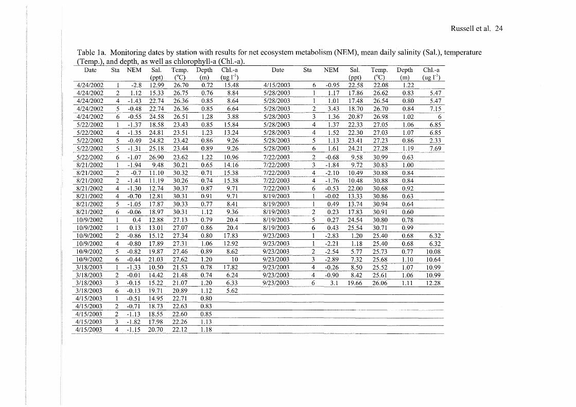
Table la. Monitoring dates by station with results for net ecosystem metabolism (NEM), mean daily salinity (Sal.), temperature (TemQ.), and deQth, as well as chloroQhyll-a (Chl.-a).

Date Sta NEM Sal. Temp. Depth Chl.-a Date Sta NEM Sal. Temp. Depth Chl.-a

(22t2 COC) (m) (ug r 1) (ppt) COC) (m) (ug r 1

)

4/24/2002 1 -2.8 12.99 26.70 0.72 15.48 4115/2003 6 -0.95 22.58 22.08 1.22 4/24/2002 2 1.12 15.33 26.75 0.76 8.84 5/28/2003 1 1.17 17.86 26.62 0.83 5.47 4/24/2002 4 -1.43 22.74 26.36 0.85 8.64 5/28/2003 1 1.01 17.48 26.54 0.80 5.47 4/24/2002 5 -0.48 22.74 26.36 0.85 6.64 5/28/2003 2 3.43 18.70 26.70 0.84 7.15 4/24/2002 6 -0.55 24.58 26.51 1.28 3.88 5/28/2003 3 1.36 20.87 26.98 1.02 6 5/22/2002 1 -1.37 18.58 23.43 0.85 15.84 5/28/2003 4 1.37 22.33 27.05 1.06 6.85 512212002 4 -1.35 24.81 23.51 1.23 13.24 5/28/2003 4 1.52 22.30 27.03 1.07 6.85 5/22/2002 5 -0.49 24.82 23.42 0.86 9.26 5/28/2003 5 1.13 23.41 27.23 0.86 2.33 5/22/2002 5 -1.31 25.18 23.44 0.89 9.26 5/28/2003 6 1.61 24.21 27.28 1.19 7.69 5/22/2002 6 -1.07 26.90 23.62 1.22 10.96 7/22/2003 2 -0.68 9.58 30.99 0.63 8/21/2002 1 -1.94 9.48 30.21 0.65 14.16 7/22/2003 3 -1.84 9.72 30.83 1.00 8/21/2002 2 -0.7 11.10 30.32 0.71 15.38 7/22/2003 4 -2.10 10.49 30.88 0.84 8/2112002 2 -1.41 11.19 30.26 0.74 15.38 7/22/2003 4 -1.76 10.48 30.88 0.84 8/21/2002 4 -1.30 12.74 30.37 0.87 9.71 7/22/2003 6 -0.53 22.00 30.68 0.92 8/21/2002 4 -0.70 12.81 30.31 0.91 9.71 8119/2003 1 -0.02 13.33 30.86 0.63 8/2112002 5 -1.05 17.87 30.33 0.77 8.41 8/19/2003 1 0.49 13.74 30.94 0.64 8/2112002 6 -0.06 18.97 30.31 1.12 9.36 8/19/2003 2 0.23 17.83 30.91 0.60 10/9/2002 1 0.4 12.88 27.13 0.79 20.4 8119/2003 5 0.27 24.54 30.80 0.78 10/9/2002 1 0.13 13.01 27.07 0.86 20.4 8/19/2003 6 0.43 25.54 30.71 0.99 10/9/2002 2 -0.86 15.12 27.34 0.80 17.83 9/23/2003 1 -2.83 1.20 25.40 0.68 6.32 10/9/2002 4 -0.80 17.89 27.31 1.06 12.92 9/23/2003 1 -2.21 1.18 25.40 0.68 6.32 10/9/2002 5 -0.82 19.87 27.46 0.89 8.62 9/23/2003 2 -2.54 5.77 25.73 0.77 10.08 10/9/2002 6 -0.44 21.03 27.62 1.20 10 9/23/2003 3 -2.89 7.32 25.68 1.10 10.64 3/18/2003 1 -1.33 10.50 21.53 0.78 17.82 9/23/2003 4 -0.26 8.50 25.52 1.07 10.99 3/18/2003 2 -0.01 14.42 21.48 0.74 6.24 9/23/2003 4 -0.90 8.42 25.61 1.06 10.99 3/18/2003 3 -0.15 15.22 21.07 1.20 6.33 9/23/2003 6 3.1 19.66 26.06 1.11 12.28 3/18/2003 6 -0.13 19.71 20.89 1.12 5.62 4/15/2003 1 -0.51 14.95 22.71 0.80 4/15/2003 2 -0.71 18.73 22.63 0.83 4/15/2003 2 -1.13 18.55 22.60 0.85 4115/2003 3 -1.82 17.98 22.26 1.13 4115/2003 4 -1.15 20.70 22.12 1.18

Russell et al. 25

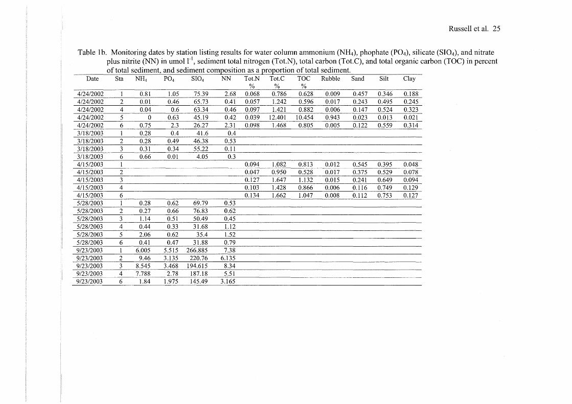
Table 1 b. Monitoring dates by station listing results for water column ammonium (NH4), phophate (P04), silicate (SI04), and nitrate plus nitrite (NN) in umol r 1

, sediment total nitrogen (Tot.N), total carbon (Tot. C), and total organic carbon (TOC) in percent of total sediment, and sediment com:Qosition as a :QrO:QOrtion of total sediment.

Date Sta NH4 P04 SI04 NN Tot.N Tot.C TOC Rubble Sand Silt Clay % % %

4/24/2002 1 0.81 1.05 75.39 2.68 0.068 0.786 0.628 0.009 0.457 0.346 0.188 4/24/2002 2 0.01 0.46 65.73 0.41 0.057 1.242 0.596 0.017 0.243 0.495 0.245 4/24/2002 4 0.04 0.6 63.34 0.46 0.097 1.421 0.882 0.006 0.147 0.524 0.323 4/24/2002 5 0 0.63 45.19 0.42 0.039 12.401 10.454 0.943 0.023 0.013 0.021 4/24/2002 6 0.75 2.3 26.27 2.31 0.098 1.468 0.805 0.005 0.122 0.559 0.314 3/18/2003 1 0.28 0.4 41.6 0.4 3/18/2003 2 0.28 0.49 46.38 0.53 3/18/2003 3 0.31 0.34 55.22 0.11 3/18/2003 6 0.66 0.01 4.05 0.3 4/15/2003 1 0.094 1.082 0.813 0.012 0.545 0.395 0.048 4115/2003 2 0.047 0.950 0.528 0.017 0.375 0.529 0.078 4115/2003 3 0.127 1.647 1.132 0.015 0.241 0.649 0.094 4115/2003 4 0.103 1.428 0.866 0.006 0.116 0.749 0.129 4/15/2003 6 0.134 1.662 1.047 0.008 0.112 0.753 0.127 5/28/2003 1 0.28 0.62 69.79 0.53 5/28/2003 2 0.27 0.66 76.83 0.62 5/28/2003 3 1.14 0.51 50.49 0.45 5/28/2003 4 0.44 0.33 31.68 1.12 5/28/2003 5 2.06 0.62 35.4 1.52 5/28/2003 6 0.41 0.47 31.88 0.79 9/23/2003 1 6.005 5.515 266.885 7.38 9/23/2003 2 9.46 3.135 220.76 6.135 9/23/2003 3 8.545 3.468 194.615 8.34 9/23/2003 4 7.788 2.78 187.18 5.51 9/23/2003 6 1.84 1.975 145.49 3.165

Russell et al. 26

Table 2. Stations sampled for net ecosystem metabolism. T. C. E. Q. descriptions and locations.

Assessment Station No. Longitude Unit Short Description Latitude (N)

(W) TCEQ UTMSI

Upper-Bay 17552 LB 1 Lavaca Bay So. of 28.69683456 96.64499664 Garcitas Cove

Upper-Bay 17553 LB2 Lavaca Bay West 28.67436218 96.58280182 of Point Comfort

Upper-Bay 13383 LB3 Lavaca Bay at SH 28.63888931 96.60916901 35

Lower-Bay 17554 LB4 Lavaca Bay East 28.63933372 96.58449554 ofNoble Point

Lower-Bay 13384 LB 5 Lavaca Bay at 'Y' 28.59583282 96.56250000 atCM 66

Lower-Bay 17555 LB6 Lavaca Bay South 28.59769440 96.51602173 of Rhodes Pt.

Table 3. Wind dependent and constant diffusion coefficient (K) equations. Diffusion coefficients (K) are in g 0 2 m-2 h-1

• Odum and Wilson; and Marino and Howarth estuarine subset equations estimated from graphs.

Author(s) Location(s) Wind Speed Equation Variability Range (m s-1

) X = Wind S2eed Ex2lained (%) Odum and Texas Gulf 0-12 0.2x NA

Wilson, 1962 Coast Marino and World Wide 0-12 0.1 098e(0.249x) 55

Howarth, 1993 Full data set Marino and Estuarine 0-12 e(l.OO + 0.4x) NA

Howarth, 1993 data subset D'Avanzo et Waquoit Bay NA 0.56e(0.15x) NA

1996 Caffrey, 2004 NERR sites 0-10 0.5 NA

Russell et al. 27

Fig. 1. Map of24 hour data sonde deployment at U. T. M.S. I. stations in Lavaca Bay.

Fig. 2a. Environmental condition PCA scores.

Fig. 2b. Environmental condition PCA loads.

Fig. 3. One way anova of chl.-a by station with Tukey's minimum significant difference=± 3.7

as error bars.

Fig. 4. Net ecosystem metabolism vs. chlorophyll-a linear regression.

Fig. Sa. Water column nutrient PCA scores (Circled area contains scores during high freshwater

inflow).

Fig. Sb. Water column nutrient PCA scores close up.

Fig. Sc. Water column nutrient PCA loads.

Fig. 6a. Sediment characteristics PCA scores.

Fig. 6b. Sediment characteristics PCA loads.

Fig. 7. Upper Bay net ecosystem metabolism vs. freshwater inflow.

Fig. 8. Lower Bay net ecosystem metabolism vs. freshwater inflow.

Fig. 9. Cumulative ten day prior to date gauged freshwater inflow into Lavaca Bay, Texas.

(Circles denote sample dates.)

Fig. 10. Mean daily salinity vs. cumulative freshwater inflow from ten days prior to sample date.

(Labeled by U. T. M. S. I. station number.)

Fig. 11. Wind dependent and constant diffusion coefficients (K) vs. wind speed.

s

o30'0"N

Lavaca Bay UTMSI Stations

96°30'0"W

4 6 8 . -------------.-- K 110 meters

96o30'0"W

Fig. 1. Russell et al.

Russell et al. 28

Russell et al. 29

3~------------------------------------------~

Lower Bay 2 6

5

N

6

6 6 6 5 2 .. ··· .. ···

6 41 3 4 : 5 '34 4 ~ ~i1 2 6

() 0 D..

4 5~ ~111~1 1

6 4

-1 6• ... · ....... 3

-2

.·· .. · .. ·· 1 3· ... 22

1<§

2

1

2

1

Upper Bay

-3+-------~----~------~------~------~----~

-3 -2 -1 0

PC 1

Fig. 2a. Russell et al.

2 3

1.0 ~-----------------------------------------.

T p

0.5

-0.5

-1.0 +-----------,.----------~----------r-----------1

-1.0 -0.5 0.0 0.5 1.0

PC 1

Fig. 2b. Russell et al.

Russell et al. 30

6 -.. 'o p = 0.5821 ~ 6 R2 = 0.007 E

N 4

0 0') 6 5 E 2

.!Q 3 0 5 ..c 24 co Q)

3 6 64 ~ 0

6t E 5 2

~ 4$ 4 2 ~ Q)

t5 5 4 2 >. (J) 2 0 -2 (..)

w 2 ....... 3 Q)

z -4

0 5 10 15 20

Chlorophyll-a (ug r1)

Fig. 4. Russell et al.

2

C\1 () 0 0..

-1

-2

2

C\1 () 0 0..

-1

3

-8 -6 -4

Upper Bay

-2 2

-2.0 -1.5 -1.0

2

-2 0

PC 1

2

Fig. Sa. Russell et al.

2 1

-0.5

1 2

22 1 .. ··

0.0 0.5

PC 1

Fig. 5b. Russell et al.

Russell et al. 31

4 6 8

Lower Bay

1.0 1.5 2.0

Russell et al. 32

0.6

0.4

0.2

N () 0.0 0..

-0.2

-0.4

-0.6 -0.6 -0.4 -0.2 0.0 0.2 0.4 0.6

PC 1

Fig. Sc. Russell et al.

Russell et al. 33

2

Lower Bay

f 4

N 3 0 0 5 0...

2

-1

Upper Bay

-2 1

-8 -6 -4 -2 0 2 4 6 8

PC 1

Fig. 6a. Russell et al.

0.8

0.6

t N 0.4

0.2

N ru 0 0.0 0...

-0.2

-0.4

-0.6

-0.8 -0.6 -0.4 -0.2 0.0 0.2 0.4 0.6

PC 1

Fig. 6b. Russell et al.

Russell et al. 34

5~------------------------------------------------~

N

0 9 2 E -~ 0 ..c ro ...... <D 0 ~

E 2 -1 (/) >. ~ -2 t)

UJ

• y = 0.0220- 1.48oo-9x

p < 0.0001

R2 =0.41

(j) -3 • z

-4+-----~----~----~----~----~----~----~----~~

0.0 2.0e+8 4.0e+8 6.0e+8 8.0e+8 1.0e+9 1.2e+9 1.4e+9 1.6e+9

Ten Day Prior Freshwater Inflow (ft3)

Fig. 7. Russell et al.

~ ~ E

N

0 9 E -~ 0 ..c ctl -(].) ~

E (].) -(/) >. (/) 0 (.)

w -(].) z

5

4

3

2

I ' • 0 • • •

-1 • • I • -2

-3

• • I

Russell et al. 35

• y = -0.2577 + 2.649e-10

p = 0.3497 •

• • •

R2 = 0.03

• • •

•

-4+-----------.-----------.-----------.-------.-----------.-----------.-----------r----------~~

0.0 2.0e+8 4.0e+8 6.0e+8 8.0e+8 1.0e+9 1.2e+9 1.4e+9 1.6e+9

Ten Day Prior Freshwater Inflow (fe)

Fig. 8. Russell et al.

.-. ("')

~ -~ 0

;:;:: c !..... Q) ...... ro ~ .c C/) Q) !.....

LL !.....

0 ·c 0... >. ro 0 c Q)

I-

1.4e+10

1.2e+10

1.0e+10

8.0e+9

6.0e+9

4.0e+9

2.0e+9

0.0

2002 2003

Date

Fig. 9. Russell et al.

Russell et al. 36

2004

-+-' Cl.

-9:: >. ~ c

-ro (/)

30

6 25

' 6 4 (J

20 ~ 4 5 6

15 2 12 ~ ~ 1

10

5

6

4 2

p < 0.0001

R2= 0.43

2

Russell et al. 3 7

0+---~----~----~--~----~--~~--~----~---4

0.0 2.0e+8 4.0e+8 6.0e+8 8.0e+8 1.0e+9 1.2e+9 1.4e+9 1.6e+9 1.8e+9

Ten Day Prior to Sample Freshwater Inflow (fe)

Fig. 10. Russell et al.

j:: C';J

E C\1

0 ~ ~

Russell et al. 38

6 ~--------------------------------------------------~

5

4

3

2

0

-- -- -- D'Avanzo et al. 1996 Marino and Howarth 1993 Full Data Set Marino and Howarth 1993 Estuarine Subset Odum and Wilson 1962 Caffrey 2004

. /

/ /

.·· / .·'/ .. -·-··-

?" .. -............-.... --- ............. _ ..... .:..-··--- ---··-.·.· .. · -----··-·· .

--=--~-:-:; _::;;; ;:_ :~= ~ ~ ~ 2 4 6 8 10 12

Wind Speed m s·1 (at 10 m height)

Fig. 11. Russell et al.