Physics 221 EXPERIMENT 6

SIMPLE HARMONIC MOTION

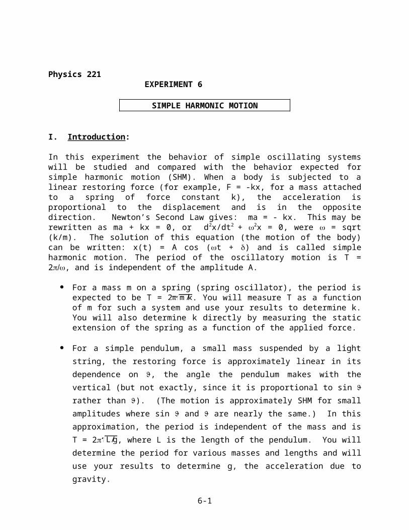
I. Introduction:

In this experiment the behavior of simple oscillating systems will be studied and compared with the behavior expected for simple harmonic motion (SHM). When a body is subjected to a linear restoring force (for example, F = -kx, for a mass attached to a spring of force constant k), the acceleration is proportional to the displacement and is in the opposite direction. Newton’s Second Law gives: ma = - kx. This may be rewritten as ma + kx = 0, or d 2x/dt2 + 2x = 0, were = sqrt (k/m). The solution of this equation (the motion of the body) can be written: x(t) = A cos (t + ) and is called simple harmonic motion. The period of the oscillatory motion is T = 2, and is independent of the amplitude A.

For a mass m on a spring (spring oscillator), the period is expected to be T = 2π m/k. You will measure T as a function of m for such a system and use your results to determine k. You will also determine k directly by measuring the static extension of the spring as a function of the applied force.

For a simple pendulum, a small mass suspended by a light string, the restoring force is approximately linear in its dependence on , the angle the pendulum makes with the vertical (but not exactly, since it is proportional to sin rather than ). (The motion is approximately SHM for small amplitudes where sin and are nearly the same.) In this approximation, the period is independent of the mass and is T = 2 L/g, where L is the length of the pendulum. You will determine the period for various masses and lengths and will use your results to determine g, the acceleration due to gravity.

II. Required Equipment: Lab Bench computer running Science Workshop and Graphical Analysis software. photogates. Pasco interface.

A. Spring Oscillator. Vertical post, crossbar, clamp and hook. Spring. Set of pendulum bobs. Meter stick. Ruler.

B. Simple Pendulum. Vertical post, crossbar, and string clamp. String and cutter for string. Set of pendulum bobs. Protractor.

III. Procedure:

6-1

A. Spring Oscillator.

1) Period as a function of mass. Use the set of three pendulum bobs as masses. Hang the spring from the stand. Hang a mass m on the end of the spring, so that the bottom of the mass is positioned just above the photogate. Make sure that the photogate is plugged into input #1 on the Pasco interface. Start the mass oscillating vertically from its equilibrium position, so that the bottom edge of the mass just passes through the photogate, cutting the light beam. Only a small amplitude is required. Avoid striking the photogate.

Photogate

Spring

M

Motion

Determine the period T of the oscillations, by running the Science Workshop program and analyzing with Graphical Analysis.

1. To measure the period, T, start up the Data studio program, by double-clicking on the Data studio icon on the Desktop. You should see the familiar Control Window and Menu Bar.

2. Click and drag the digital plug icon to digital channel 1 to logically connect the photogate to that channel. From the pop-up timing menu, scroll down and select “photogate and picket fence”.

3. Create the data table and graph by dragging the little table and graph icons to the same channel as you did the plug, and selecting “period(t)” to display for each. In the table heading, click on the [0.00...] button and select 4 digits to be displayed.

4. Start the motion and record at least N = 20 time measurements.5. Click on the Stop Button.6. Select the data column in the table and click the [] symbol to obtain mean (T) and standard

deviation (T) values, and N = number of measurements. Record these values. (note: T = (T)/ N ).

7. Repeat the process until you have made measurements for all three pendulum bobs of different mass. For each pendulum bob, determine its mass and estimate the error (m). Also measure and record the mass of the spring.

Graphical Determination of the Spring Constant (k).

1. Open Graphical Analysis, from Recent Applications or from the desktop. In the blank table which appears, label successive columns and enter your three mass values (M in kg), the corresponding period (T in sec), and the square of the period (T2 = T^2).

2. From the Graph Menu, turn on Regression Statistics. Plot T2 versus M. The errors in the T2 values and M values are sufficiently small that you can ignore them.

3. The slope of the regression (straight) line should be numerically equal to (42)/k. The error in the slope (slope) can be obtained from the regression statistics.

6-2

4. From the slope we can now write: k = (42)/slope. The error in k can be obtained from the expression: k/k = slope/slope.

5. Print a copy of this graph for each group member, including regression statistics. Record values of slope, slope, k, and k in your lab report form.

2) Hooke's Law: Static Extension as a Function of Mass. We can also measure the spring constant (k) from static extension of the spring, and compare the value of k so obtained with that of the dynamical measurement above.

1. Use the three masses used above. For each, measure the static extension Y of the spring as a function of the weight W = mg which is hung from it.

2. Estimate the error Y in your measurements of Y.3. Using Graphical Analysis, plot the static extension Y of the spring as a function of the

weight W = mg. Include error bars on the Y values; you may assume the errors in m and thus in W are negligible.

4. A straight line relationship would verify Hooke's Law for the spring. Make sure Regression Statistics is selected under the Graph Menu. The slope of the line should be Y/W = (1/k) and the error in the slope (slope) will be given from the Regression Statistics.

5. From this result, we may determine the force constant from the expression k = 1/slope and its error from k/k = slope/slope.

6. Print out a plot of your data with the Regression Statistics for each group member. Record k, k, slope, and slope in your physics lab report form.

B. Simple Pendulum

1) Period as a function of mass.

Use the three pendulum bobs of identical size but different mass in this part of the experiment. Keep the amplitude m of the swings smaller than about 20o and try to use the same amplitude for your repeated measurements. do not let the pendulum strike the photogateMake a simple pendulum roughly 50 cm long from a piece of string and one of the pendulum bobs. Measure the length L (from pivot point to center of mass) and estimate the error L in your length measurement. You will measure the periods at small amplitude for this pendulum and the other two pendulum bobs of different mass, being careful to keep the length constant when you change the bob. Data for Simple Pendulum

1. Double-click on the Science Workshop icon on the computer desktop (i.e. screen). If Science Workshop is already open, select New under the File menu. A Control Window with a Menu Bar across the top should appear on the screen.

6-3

2. Click and drag the digital plug image to the digital channel into which the photogate is connected to logically connect the photogate to that channel. From the pop-up timing menu, scroll down and select “photogate and pendulum”.

3. Create the data table and graph by dragging the little table and graph icons to the same channel as you did the plug, and selecting “period(t)” to display for each. In the table heading, click on the [0.00...] button and select 4 digits to be displayed.

4. Start the pendulum oscillating, by pulling it sideways several inches and releasing it.

5. Now Click on the [REC] button in the Control Window to begin data recording. The graph will update dynamically in real time as the data taking progresses. Depending upon conditions, you may be able to record 30 to 50 oscillations . Then click on the “Stop” button.

6. Select the data column in the table and click the [] symbol to obtain mean (T) and standard deviation (T) and number of measurements (N). Record these values .

(note: T = (T)/ N ).

7. Repeat the above procedure for the other bobs and enter these data in your data table.

2) Period as a function of length Using the bob of intermediate mass, determine T for 3 or more different pendulum lengths L. Cover as wide a range of L as possible. Adjust the position of the string clamp so that the bob intercepts the photogate. (Again, keep the amplitude reasonably small and fairly constant.) Your measurement from part B1 using this bob can be one of the measurements. Measure L and estimate the error L in each case. (A single length error will suffice for all the measurements unless you have reason to believe different errors are needed.)

Record about 30 oscillations for each length, using the same procedure as above. Record the mean (T) and standard deviation (T) for each pendulum length in a data table.

Use the values from this data table for this part. In Graphical Analysis, select New under the File menu and make 5 more columns. The first 5 columns will be L, T, (T), N and

6-4

T = (T)/ N . Next 2 columns will be set up as T2 and

6-5

T 2

6-6

(where T2 = 2TT) using the same procedure as in A1.

Plot T2 versus L , Include vertical error bars on the T2 values, with magnitude T2. Turn on Regression Analysis to get the slope and its error. Make a Print Screen for each partner.

6-7

From the equation T = 2 L/g expected for SHM, we see that T2 = (42/g)L and the slope T2/L of the T2 versus L line should be 42/g, the error in the slope is

6-8

(4 2 g2 )g6-9

. Thus g = 4 2/slope and g/g = slope/slope.

NOTE: You have now completed all the necessary in-class work. Before you leave the laboratory make sure you have made all the required measurements and estimates of errors needed to complete the experiment. Get your instructor to initial your work.

IV. Analysis and Discussion:

A. Spring Oscillator.

Are your results consistent with the variation of period with mass which is expected from theory? Discuss the evidence for your conclusion. Was Hooke's Law obeyed for the spring you used? Discuss the evidence for this. Compare the two values of the spring constant k which you found. Compute the difference and the error in the difference. Do the two values agree? If not, can you think of any possible reasons for the difference? What was the value of the intercept in your plot of T2 versus m? Do you expect T=0 when m=0? Discuss this briefly.

B. Simple Pendulum

1) Period as a function of mass.

Are your measurements of T for the three pendulum bobs of different masses consistent with the period being independent of the mass?

2) Period as a function of length.

6-10

Calculate a value for g and

6-11

g

6-12

using your fit results. Compare the value of g you obtain with the standard value. Ar they consistent? If not, can you think of any possible reasons for the difference? Also determine the intercept (the value of L for which T2 = 0) and the error in he intercept. What would you expect t

TABLE 1. DATA ON Spring Oscillator

6-13

BOB ID M=mass of the bob (kg)

T= period (sec)

T(s)6-14

1

2

3

6-15

mspring =6-16

TABLE 2. DATA ON Hooke’s Law

mass hung (kg) extension, x (m) F=mg (N)

1

2

3

4

5

6-17

x =6-18

TABLE 3. DATA ON Pendulum (length kept constant, mass varied)

6-19

BOB ID mass of bob T= period (sec)

T(s)6-20

1

2

3

TABLE 4. DATA ON Pendulum (mass kept constant ,length varied)

6-21

BOB ID length L (m) T= period (sec)

T(s)6-22

1

2

3

6-23

6-24

L =6-25

6-26