Paper ID #12001

A Simple Hands-On Experiment for First Year Undergraduates that Con-nects the Electrical and Thermal Properties of Metals

Dr. Kathleen Meehan, University of GlasgowProf. Robert H Hadfield, University of Glasgow, UK

Robert Hadfield is Professor of Photonics and Head of the Division of Electronic and Nanoscale Engi-neering at the University of Glasgow, United Kingdom.

Andrew Phillips

c©American Society for Engineering Education, 2015

Page 26.109.1

A Simple Hands-On Experiment for First Year Undergraduates

that Connects the Electrical and Thermal Properties of Metals

Abstract

The undergraduate engineering programmes at the University of Glasgow were recently revised

to include a common core of classes in Year 1 and Year 2. Materials I, an introductory materials

science course, is now taken by all Year 1 engineering students. The lectures in the course were

modified to include topics that are of interest to electronic and electrical engineering students,

electrical and optical properties of materials. A hands-on laboratory experience has been developed

to support student learning on electrical resistivity and thermal conductivity. The hands-on

experiment about optical reflectivity will be added to the laboratory in the near future. This paper

describes the laboratory exercise – the intended learning outcomes, the laboratory procedure, an

evaluation of the student performance, and a discussion on improvements that will be made to

increase student understanding of the topics and ancillary subjects.

I. Background on Hands-On Learning in Materials Science

Many institutions of higher learning have adopted a common set of engineering and science

courses into their engineering degree programmes, where an introductory materials science course

is often one of the core courses. Recognizing the universality of certain experiences (snapping a

metal paperclip as a result of cold working, for example), routine choices that involve material

selection (purchase of a bicycle is driven by cost. weight, and material composition), and the fun

that student can have making and destroying objects while learning concepts from materials

science, measuring material properties, and designing structures that rely on the proper selection

of materials, educators have designed hands-on laboratory exercises that allow students to explore

the properties of materials and how their knowledge of these properties can guide the selection of

materials for specific applications1

23

–4

5.

However, an issue that arises when reviewing the lab exercises is that the concepts that are

demonstrated during these labs tend to emphasize the mechanical and thermal properties of

materials. While these concepts are useful for all engineering students to understand, few of the

experiments explore and emphasize the concepts about and the relationships between the electrical,

optical, and magnetic properties of materials67. These concepts have more immediate relevant to

students in electronic, electrical, and computer engineering and are increasingly important to

students in all fields as microcontrollers and sensors are pervasive elements in almost all

engineering designs. Hence, there is a need to design hands-on activities in these materials science

courses that expose students to the non-mechanical properties of materials.

II. Course Redesign at the University of Glasgow

The inclusion of materials science into the core engineering courses taken by undergraduate

students in Electronic and Electrical Engineering (EEE) at the University of Glasgow occurred

during the restructuring of all of the engineering programmes in 2012. This prompted a review of

Page 26.109.2

the instructional materials by the staff to ensure that topics relevant to the discipline-specific

courses taken later in the EEE students’ academic careers were introduced to students during this

Year 1 one-semester course without significantly decreasing the instruction on topics that are

needed by students in other engineering programmes. As a result of the review, the course was

revised and additional lectures on the electrical, optical, and magnetic properties of materials along

with discussions about the requirements for the materials used in electronics such as solar cells,

high speed transistors, and magnetic storage were inserted into the course.

The first cohort of Year 1 students took the revised course in Fall 2013. While the students in

general gave the course high marks in the end-of-semester course evaluation, a number noted that

one aspect of the course did not contain any material related to EEE – the labs still were traditional

experiments on the strength of materials. This was not an oversight by the staff involved in the

course revision; the time required to revise the lectures precluded the development of a new

experiment on the electrical, optical, and magnetic properties of materials.

After the course was taught for the first time, attention was shifted to the development of a lab

exercise in which students would apply some of the concepts on the electrical and optical

properties of metals presented in lectures. Since the electrical, optical, and thermal properties of

metals are related to the concentration of electrons in the ‘sea of electrons’ and the electron-

electron and electron-lattice interactions, it was decided to design a lab that allowed students to

measure these properties and determine experimentally the relationships between the properties.

III. Experimental Apparatus

Constraints on the development of the lab were the usual ones – space, cost, time, and safety. The

electronics lab classrooms were the only rooms available to host the new materials lab. Since one

of the measurements was the electrical resistance of lengths of wire, the digital multimeters that

were located at each laboratory station could be used. However, the experimental apparatus

required for the thermal and optical characterization of metal samples did not exist. Thus,

additional lab equipment had to be purchased or developed. It was decided that the electronic

laboratory staff would design the apparatus such that it met the following general constraints. The

apparatus had to fit on the lab benches and be portable so that it could be removed when the rooms

would be used for electronics labs. Thus, the apparatus had to have a small footprint and,

preferably, would require only the measurement equipment already at the benches. To limit the

cost of running the new lab, the apparatus and the consumables were designed to last for multiple

years. Lastly, the apparatus had to be available in time for the scheduled lab sessions. After

reviewing the schedule for the design and testing of initial prototypes and a build cycle for the 40

sets of apparatus needed to supply each lab session, it was agreed to concentrate efforts on the

design of the apparatus required for the experimental determination of the thermal properties of

metals. The design of the apparatus for the reflectivity measurements would be delayed and the

experimental determination of the optical properties of metals would be added to the laboratory

procedure in 2015.

To determine the thermal conductivity, the apparatus required had to heat metal samples while

students made measurements of the sample’s temperature. Thus, the design requirements for this

specific piece of equipment were as follows. There had to be a hot surface of relatively uniform

Page 26.109.3

temperature upon which a block of metal would sit. The hot surface had to be held at a fixed known

temperature during the experiment. Thus, a provision for a measurement of the heat sink

temperature should be incorporated into the design. The opposite surface of the metal block to the

one on the heat sink had to be accessible for temperature measurements.

A 100 Watt power resistor with integrated heat sink (Arcol HS100 Series, 15Ω ± 5 %) was used

as the source of thermal power. The maximum temperature that the surface of the heat sink could

reach was 100 oC when the power resistor dissipates 100 W when the integrated heat sink is

secured to a secondary heat sink. It was decided that the safety precautions, which would be needed

to prevent accidental burns, were too onerous at this temperature. Thus, it was decided that thermal

control would be design to limit the temperature of the heat sink to nominally 50 oC. Students

would be provided tweezers to move the metal blocks between a thermally isolated storage bin

and the hot surface of the heat sink to further limit the potential for accidental burns. As a safety

measure, a thermal switch was added to the design to insure that power to the resistor would be

disconnected should the temperature of the heat sink exceed 70 oC.

The thermostat that was designed to regulate the temperature of the power resistor’s heat sink was

a bang-bang controller; the layout of the printed circuit board (PCB) for the thermostat is shown

in Figure 1. Feedback to the thermostat circuit was provided by a resistance measurement a

thermistor (RS 10 kΩ NTC, type E95) mounted to the top surface of the heat sink near the location

where the metal blocks would be placed. It was experimentally determined that the controller could

regulate the temperature of the heat sink of the power resistor to within +/- 1 oC once steady state

operation was reached. However, there was a lengthy warm-up time as the drive current to the

power resistor was restricted to a maximum of 0.8 A, the maximum current that the 12V AC-to-

DC adaptor used as the power supply for the apparatus could drive through the 15 power resistor.

The circuit had to be turned on for approximately 20 minutes before the apparatus was ready for

use by the students. As students would perform the measurements needed to calculate electrical

resistance prior to the measurements needed for the calculations of thermal conductivity and

specific heat capacity, the warm-up time was acceptable as long as the apparatus was turned on at

the beginning of the lab session.

A power switch was integrated into the circuit along with two LED indicators, a yellow LED to

show that power was supplied to the power resistor and a green LED to show that the temperature

of the heat sink was within the desired temperature range. There was overshoot in temperature of

~ 0.5 oC before a steady-state temperature of nominally 50 oC was maintained. Given the minimal

temperature overshoot, the thermal control provided by the bang-bang controller was sufficient to

provide a well-regulated heated stage for the experiment.

Measurements were made of the temperature uniformity across the surface of the heat sink. The

results were used to select the width of the metal blocks that would be in contact with the heat sink

on its narrower dimension. The maximum width of the metal blocks such that there was a 1 oC

change in the temperature of the surface of the heat sink was 5/8”, which was sufficiently large to

allow easy handling of the blocks with the tweezers. The depth of the blocks was chosen to be the

same dimension. The length of the blocks was determined after an analysis of the transient

response of various metals when heated under these conditions. To insure that students placed the

metal blocks on the center of the heat sink, a square hole in the thermostat circuit PCB was aligned

Page 26.109.4

over the heat sink of the power resistor. The square hole can be seen in the lower left corner of the

PCB in Figure 1. Mechanical stand-offs were used to prevent contact between the PCB and the

heat sink.

In addition to the thermistor mounted to the power resistor heat sink, three thermistors were wired

to banana jacks on the PCB, which are located on the right side in Figure 1. Each thermistor was

epoxied to the top surface of one of the metal blocks used in the section of the experiment on the

thermal properties of metals. The banana jacks allowed students to easily switch between

thermistors when measuring the resistance of the heat sink and of the metal block under test.

A total of 40 printed circuit boards were constructed at a cost of £55.78 per printed circuit board.

The cost included the components. The assembly and testing of the PCBs was done in-house. The

40 spools of Al, Cu, and Fe wire were ordered from Crazy Wire and Wire.co.uk at a total cost of

£142.90. The bar stock of Al and Cu used to fabricate the metal blocks for the thermal conductivity

and heat capacity measurements were ordered from John Hood (£28). The bar stock were

machined into 5/8”x 5/8” x 3/4" blocks in-house. All costs provided do not include the value-added

tax (VAT). The reliability of the apparatus was good. Only one repair during the semester was

required on a board, found during the second laboratory session. We speculate that the board was

Figure 1: Printed circuit board (6” x 6”) for a temperature-controlled heated stage with a ¾” x ¾” mask for samples (yellow square on lower left), plug for ac-to-dc adapter on upper left, and banana jack plugs for thermistors to monitor temperature of the heat sink and metal blocks.

Page 26.109.5

accidentally not tested after assembly. There were no other failures of the PCBs during the seven

laboratory sessions.

IV. Intended Learning Outcomes

The purpose of the laboratory was to provide students with practical experience on the

measurements and calculations used to determine the electrical and thermal properties of metals.

From this and other intended learning outcomes of the experiment, students should be able to:

Calculate the diameter of a metal using the measurement of electrical resistance when given

the length of the metal sample.

Determine the electrical resistivity of an unknown metal from the relationship between

measured electrical resistance of a metal sample of known length and calculated diameter.

Use the measured temperatures of a metal sample and its dimensions to determine the

power per area transmitted from a heated surface to the metal.

Determine the thermal conductivity of an unknown metal from the relationship between

the calculated power per area delivered to one surface of metal, the maximum temperature

of the opposite surface of the metal, and the dimensions of the sample.

Use look-up tables, which are either provided or must be found by the student, to determine

wire gauge, electrical resistivity, thermal conductivity, and temperature.

Fit a set of data to an exponential function using the built-in macro in Microsoft Excel.

Calculate the specific heat capacity of aluminum (Al), copper (Cu), and an unknown metal

using thermal conductivities, the lengths of the samples, and the exponential exponent

obtained from Excel.

Identify the unknown metal by comparing the calculated electrical resistivity, thermal

conductivity, and specific heat capacity from a subset of metals, provided to the students.

Use the relationship between the ‘sea of electrons’ and the electrical and thermal properties

of metals, which is described in the Wiedemann-Franz law, to calculate the Lorenz number.

Explain the accuracy of the identification of the unknown metal through an evaluation of

uncertainties calculated for the electrical resistivity and thermal conductivity of the metal,

the calculated values for specific heat capacities and the Lorenz numbers for Al and Cu.

Identify potential sources of errors in their experimental measurements.

V. Scaffold of the Experimental Procedure

The lab procedure was written to be a stand-alone document. This was, in part, necessary because

the course textbook, Materials Science and Engineering: An Introduction by Callister and

Rethwisch, is recommended rather than required. In addition, the laboratory sessions were

scheduled to be held throughout the semester because of the number of laboratory sessions that

were required for the 275 students in the course coupled with the availability of the laboratory

classroom and instructors. Thus, some of the students performed the lab before the material

introduced in the course lectures; although most of the students performed the lab after the lectures

were completed.

The document was written in four sections. A general description of the structure of each section

is provided here. First, general background on the origins of the ‘sea of electrons’ is given followed

by a brief mention of orbital hybridization. Two metals, Al and Cu, are used as examples. The

Page 26.109.6

experimental procedure is then divided into three sections: electrical properties of metals, thermal

properties of metals, and the relationship between the electrical and thermal properties. The

experimental procedure will be expanded to include the theory on the optical properties of metal

with emphasis on reflectivity in the near future and the last section will be revised to include the

relationship between electrical and optical properties in the future. Within each of the sections on

electrical and thermal properties of metals, the theoretical concepts that relate the material from

the general background to the specific material property are presented. As the measurements that

the students will perform are influenced by the physical geometry of the samples, the equations

that connect the measured quantities of electrical resistance, temperature, and time with the

fundamental material properties of electrical resistance, thermal conductivity, and molar heat

capacity are given. Then, the steps that the students must perform to make the measurements on

two known and one unknown metal samples and the calculations using the measured quantities

were provided. The specific steps carried by students in each of the last three sections of the

experimental procedure are described more completely below. At appropriate points after certain

calculations, students are asked to identify the metal of the unknown sample by comparing the

calculated electrical and thermal resistivities and specific heat capacity of the unknown metal with

the accepted values of each of these material properties for the metals and other materials that are

provided in tables in the procedure. Students must also determine the uncertainties associated with

each of the calculated material properties. In the final section of the laboratory procedure, the

connection between the electrical and thermal properties, as given by the Wiedemann-Franz Law,

is described. The students are asked to calculate L, the Lorenz number, using the experimental

values for resistivity and thermal conductivity. As a final step, students are asked to comment on

the accuracy of the calculated values of resistivity, thermal conductivity, and specific heat capacity

and how this may have affected the identification of the unknown metal.

Additional material provided in the laboratory procedure were a periodic table to support the

discussion in the second on general background, a table of electrical resistivities and a table of

thermal conductivities and specific heat capacities for a selection of metals and other materials,

Table I and II, respectively. Lastly, a lookup table of thermistor resistances and temperature was

also provided. A worksheet was also devised and distributed to students at the beginning of the

laboratory session for data entry, the results of their calculations, and comments.

a. Experiment Procedure: Resistivity and Resistance

In this section, the relationship between the concentration of electrons in the ‘sea of electrons’, the

mobility of the electronics, and the electrical resistivity of the metal is presented. As the

measurable quantity is electrical resistance, the relationship between electrical resistivity and the

physical geometry of the metal is described.

Students are given three lengths of wire. The metal used to fabricate two of the wire samples are

known – a 60 m length of aluminum wire coated with green enamel and a 90 m length of copper

wire coated with blue enamel. They are also given a 20 m length of iron wire coated with orange

enamel. The students are told the composition of the Al and Cu wires and the relationship between

the average of the diameters of the Al and Cu wires and that of the unknown wire, which was 1.6

times larger. The difference in diameter between the known wires and the unknown wire was due

to the availability of the materials; however, the diameter of each of the wires is not given. The Page 26.109.7

lengths of each of the wires are also provided to the students as measurement of these lengths of

wire would have been too difficult.

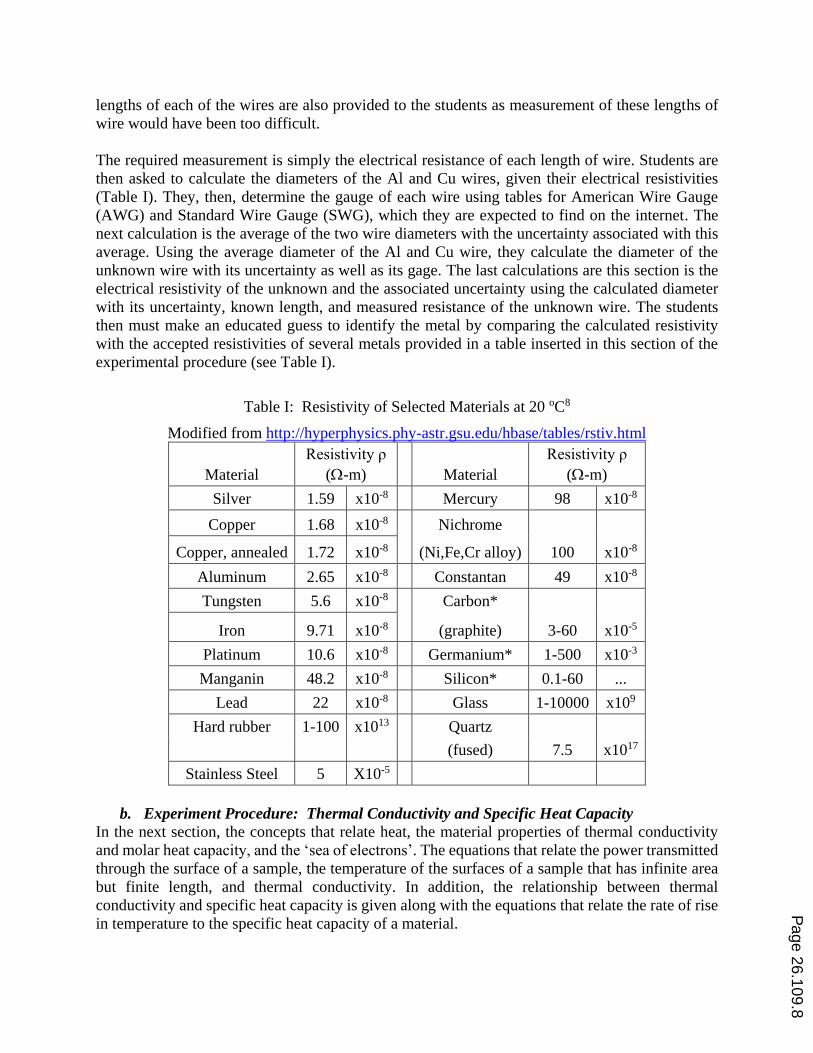
The required measurement is simply the electrical resistance of each length of wire. Students are

then asked to calculate the diameters of the Al and Cu wires, given their electrical resistivities

(Table I). They, then, determine the gauge of each wire using tables for American Wire Gauge

(AWG) and Standard Wire Gauge (SWG), which they are expected to find on the internet. The

next calculation is the average of the two wire diameters with the uncertainty associated with this

average. Using the average diameter of the Al and Cu wire, they calculate the diameter of the

unknown wire with its uncertainty as well as its gage. The last calculations are this section is the

electrical resistivity of the unknown and the associated uncertainty using the calculated diameter

with its uncertainty, known length, and measured resistance of the unknown wire. The students

then must make an educated guess to identify the metal by comparing the calculated resistivity

with the accepted resistivities of several metals provided in a table inserted in this section of the

experimental procedure (see Table I).

Table I: Resistivity of Selected Materials at 20 oC8

Modified from http://hyperphysics.phy-astr.gsu.edu/hbase/tables/rstiv.html

Material

Resistivity ρ

(-m) Material

Resistivity ρ

(-m)

Silver 1.59 x10-8 Mercury 98 x10-8

Copper 1.68 x10-8 Nichrome

100 x10-8 Copper, annealed 1.72 x10-8 (Ni,Fe,Cr alloy)

Aluminum 2.65 x10-8 Constantan 49 x10-8

Tungsten 5.6 x10-8 Carbon*

3-60 x10-5 Iron 9.71 x10-8 (graphite)

Platinum 10.6 x10-8 Germanium* 1-500 x10-3

Manganin 48.2 x10-8 Silicon* 0.1-60 ...

Lead 22 x10-8 Glass 1-10000 x109

Hard rubber 1-100 x1013 Quartz

7.5 x1017 (fused)

Stainless Steel 5 X10-5

b. Experiment Procedure: Thermal Conductivity and Specific Heat Capacity

In the next section, the concepts that relate heat, the material properties of thermal conductivity

and molar heat capacity, and the ‘sea of electrons’. The equations that relate the power transmitted

through the surface of a sample, the temperature of the surfaces of a sample that has infinite area

but finite length, and thermal conductivity. In addition, the relationship between thermal

conductivity and specific heat capacity is given along with the equations that relate the rate of rise

in temperature to the specific heat capacity of a material.

Page 26.109.8

Students first measure the dimensions of the samples – two known blocks of metal, one composed

of Al and the other of Cu, and a third block of metal. Again, the composition of the third block is

not disclosed; students must identify the metal after determining its thermal conductivity and heat

capacity. The unknown metal is the same metal as the unknown metal that the students identified

in the previous section, which is necessary if the students are to calculate the Lorenz number for

the unknown metal.

The students then measure the rate at which blocks of Cu, Al, and the unknown metal reached a

steady-state temperature after being placed on the heated stage. After recording the resistance of a

thermistor epoxied to the surface of the power resistor’s heat sink, the students place one of the

metal blocks on the center of the heat sink. Working in pairs, students record the resistance of a

thermistor, which has been epoxied to the top surface of each metal block, every 30 seconds until

the top surface of the block has reached a steady state temperature. Once one measurement is

completed, the students remove the metal block from the heat sink and repeat the process with the

next block until measurements have been made on all three blocks of metal. The students are

provided with a lookup table to relate the thermistor’s resistance to temperature.

Table II: Thermal Conductivities and Specific Heat Capacities of Selected Materials9,10

From Callister & Rethwisch, Materials Science and Engineering: An Introduction Wiley 9th

Edition, Appendix B and www.engineeringtoolbox.com

Material Thermal Conductivity

(W/m-K)

Specific Heat

(J/kg-K)

Density

(g/cm3)

Silver 428 235 10.5

Copper 338 385 8.79

Cooper, annealed

Aluminum 6061 180 896 2.7

Tungsten 155 138 19.2

Iron 36 544 7.87

Platinum 71 132 21.5

Manganin 22 406 8.4

Hard rubber 0.14 2010 1.2

Mercury 8.69 140 13.6

Nichrome (Ni, Fe, Cr, alloy) 11.3 450 8.4

Constantan 19.5 390 8.89

Carbon (graphite) 130 830 2.09-2.23

Germanium 5.32

Silicon 141 740 2.33

Glass 1.4 840 2.2-5.9

Quartz (fused) 1.4 740 2.65

Stainless Steel 304 16.2 500 7.75-8.05

Using the maximum and minimum temperatures of the block of metal and the thermal

conductivities of Al and Cu (Table II), the calculated power per area transferred to the metal blocks

Page 26.109.9

can be calculated. Students average of the power per area and determine the uncertainty associated

with this value. Students then calculate the thermal conductivity of the unknown metal and the

uncertainty using the maximum and minimum temperatures that were measured as the unknown

metal was on the heat sink. Students compare the calculated thermal conductivity of the unknown

metal with the thermal conductivities for the metals listed in the second table (see Table II) to

identify the composition of the unknown block.

The students are then asked to fit the temperature vs. time data to an exponential expression using

Excel for each of the blocks of metal. They calculate the specific heat capacities from the

exponents for Al, Cu, and the metal that was identified from the previous calculations of thermal

conductivity. The students are asked to compare the calculated specific heat capacities with the

accepted specific heat capacities of Al, Cu, and the metal listed in Table II. They are also asked to

compare the specific heat capacity of the unknown metal to the list to determine if there is another

material listed in the table (Table II).

c. Experimental Procedure: Wiedemann-Franz Law

In the final section of the laboratory procedure, a brief explanation of the Wiedemann-Franz Law

is given along with the equation to calculate the Lorenz number from the electrical resistivity and

thermal conductivity. Students calculate the Lorenz number using the accepted material properties

for Al and Cu. The students are told at this point that the wire and block are composed of the same

metal. They then calculate the Lorenz number and the associated uncertainty for the unknown

metal. Lastly, students explain whether they think that their identification of the unknown metal is

accurate and reasons why the identification may be incorrect.

VI. Results

a. Student Preparation

During a conversation with the course instructor for Electronic Engineering 1X, a course taught to

Year 1 students in the same semester as Materials I, we learned that students were no longer

engaged in hands-on laboratories, but were running simulations using PSpice instead. Thus, a set

of instructions on how to make resistance measurements was written shortly before the first

laboratory session.

The laboratory procedure was not available to the students in the first laboratory session until they

arrived in the lab classroom. It was posted on the course Moodle site earlier that day. Nonetheless,

most students in that lab session as well as the subsequent lab sessions completed the experiment

within two hours, the amount of time time-tabled for this experiment. All of the students were able

to make the measurements described in the experimental procedure with minimal guidance from

the laboratory demonstrators (2 to 3 graduate students per lab session). Although no data was

collected to support the following opinion, it was felt that the length of the write-up (14 pages in

total, not including the worksheet or the instructions on the measurement of electrical resistance)

discouraged students from reading the laboratory procedure prior to their lab class. As it is unlikely

that the course textbook will be required in future semesters, the volume of background material

for this laboratory experiment will continue to be needed. It is possible that some of the material

will be incorporated into the course lecture notes, which would mean that the laboratory procedure

could be condensed.

Page 26.109.10

b. Grading

As is general practice in all of the engineering laboratories, each student was required to bring an

experimental laboratory notebook to this laboratory class to log data and to write observations.

Given the number of students in the course (275), a method to reduce the amount of time to grade

the student work was needed that also eliminated the constraint of collecting and returning student

laboratory notebooks in time for the second Materials I experiment on the mechanical properties

of metals. Rather that grading each lab notebook or requiring that each student write a lab report,

each student was expected to submit a worksheet for this experiment, even though they worked in

pairs when collecting the experimental data. The worksheet was designed with specific locations

for students to enter data, the results of their calculations, the educated guess of the unknown metal,

and their comments about the accuracy of the identification of the metal and the causes of the

uncertainty associated with several calculations, written in MS Word. This eliminated the need to

search through the students’ lab notebooks or through lab reports to locate the work upon which

they would be graded.

After grading the worksheets submitted by the students in the first laboratory session, it was found

that there were large variations in measurements, errors in calculations, wrong numbers found

from lookup tables, and incorrect identification of the unknown metal. All of which contributed to

make grading very difficult, even with worksheet. An Excel spreadsheet was created to reduce the

time required to grade each worksheet. Twenty four measurements were entered from the student

worksheet – resistances of the three samples of wire, the minimum and maximum resistance of the

thermistors attached to each metal block, the exponent from the exponential fit of data in Excel,

and the dimensions of the blocks of metals. (Note that each block was nominally the same

dimension as the other two so these numbers were not changed unless there was a measurement

error by the student. The results of the calculations were displayed so that the grader could verify

that the student calculations were correct. Using the results that the students should have

calculated, the identity of the metal was found using a lookup table embedded in the Excel

spreadsheet. While still time-consuming, this did simplify grading as the propagation of errors

from an initially incorrect measurement leading to the wrong identification of metals was tracked

automatically.

We are considering incorporating the worksheet as a quiz in Moodle, a virtual learning

environment11, and to have the calculated results and identification of metals graded automatically

without any assistance of a grader. As there are computers at each lab station, students would be

able to electronically enter the measurements. We have to determine if each student will have to

electronically enter the data or if there is a way to share the entered data on Moodle between the

pairs of students. Furthermore, it is not clear if there is an easy way to incorporate a lookup table

into the quiz format that will allow automatic grading of the identification of the unknown metal.

Nevertheless, we expect to be able to use quizzes in Moodle to reduce, if not entirely eliminate,

the need for graders to review the student work.

c. Analysis of Student Work

i. Electrical Resistivity

Out of 275 students enrolled on the course, 265 completed the experiment and submitted

worksheets. When comparing the accuracy of the student calculations on all sections of the

experiment, the calculations performed to find the diameters of the Al and Cu wires and the

Page 26.109.11

electrical resistivity of the unknown metal wire, were the most accurate. The results of our

evaluation of student performance in this section of the experiment are shown in Figure 2. A

description is provided below along with comments on student errors and a systematic error in

measurement.

A common error in the calculation of the diameters of the Al and Cu wires appears to have been

the use of an incorrect equation for area of a circle [ 𝜋𝑟2 = 𝜋𝑑2/2 instead of 𝜋(𝑑 2⁄ )2], which led

to an incorrect calculation diameters, resistivity of the unknown metal, and finally to an incorrect

identification of the metal. However, an exact determination of the reasons for all of the errors in

the calculation of the electrical resistivity of the unknown metal wire using their measurements of

resistance could not be deduced as students were not required to show their calculations on the

worksheet. There were four instances (1.5 %) where students identified stainless steel, which

appears to the result of incorrect reading of the range on the digital multimeters.

While only 58 students (21.9 %) correctly identified the unknown metal as iron, there was a

systematic error in the measurement of resistance that caused 158 students (57.5 %) to identify the

metal as platinum and 2 students (0.7%) who identified the metal as silver instead. The error was

likely caused by the difficulty in making good contact between the metal wires with the probes of

the multimeter as the wire gauge for the Al and Cu wires was 24 (AWG)/25 (SWG) and the fact

that the bare ends of the Al wires oxidized rapidly. Thus, the resistance of the Al wire in particular

was larger than it theoretically should have been, which caused the calculated resistivity of the

unknown block to be smaller than it was in actuality. Soldered connectors to the ends of the metal

wires will be added before the next offering of the laboratory to eliminate both of these sources of

error.

Figure 2: Assessment of student work for the calculation of resistivity of the unknown metal,

identification of the unknown metal from its electrical resistivity (), calculation of thermal

conductivity (), and calculations of the specific heat capacity (Cp) of the three metal blocks.

Page 26.109.12

While these results indicate that there was a high level of success on this section of the experiment,

there was some evidence that some students either misread the information on Table I or concluded

that their calculations were incorrect and selected either iron or platinum, likely after hearing that

other students had identified one of the two materials for the unknown metal. When taking this

into account, 167 students (60.7 %) calculated the resistivity of the unknown material correctly

using their experimental data and the electrical resistivities of Al and Cu and 159 of the 167

students (95.2 % or 57.8 % overall) used their calculated results to identify the appropriate metal.

Lastly, a total of 6 students (2.2 %) did not perform the required calculations, although they had

written resistance measurements on the worksheet and 7 students (2.5 %) did not attempt to

identify the metal.

We note that, in the assessment of student work, credit was given to students who calculated the

electrical resistivity of the unknown metal correct using their resistance measurements and

additional credit was given if the students then selected the most appropriate metal from the list in

Table I, even if the metal selected was not iron. Credit was not given to those students who

identified the metal as iron, but whose calculations of resistivity did not support that conclusion.

ii. Thermal Conductivity and Heat Capacity

We knew prior to running the experiment that there would be considerable errors in the

measurements. First, the blocks were of finite cross-sectional area. Secondly, there were

convective losses. Furthermore, there was a gradient in temperature across the heat sink and, thus,

the power transferred to the block was dependent on the exact placement of the block on the heat

sink. We had attempted to minimize gradient in temperature by masking of all but the center region

of the heat sink so that each block was placed in the same location on the heat sink (see square

opening in lower left in Figure 1). In the future, the blocks will be placed in an insulating sleeve

to prevent heat loss from the sides of the blocks. Cooling of the power resistor heat sink when the

metal blocks were placed on its surface was a concern, but was determined to be a small effect

experimentally. No noticeable change in the heat sink temperature was observed when each of the

metal blocks was placed on its surface.

Unfortunately, it became clear that there was a significant flaw with the design of this portion of

the experiment, which we had not recognized when characterizing the experimental apparatus used

in this section of the experiment. After analyzing the data collected by the students, it appears that

the measurement of thermal conductivity and heat capacity were dominated by the temperature

rise of the thermistor epoxied to the metal blocks rather than by the metal blocks themselves. The

epoxy chosen for the experiment should have been an adhesive with a high thermally conductivity

instead of a general-use epoxy. Moreover, the shape of the thermistor was not optimal and one

with a flat bottom surface and small volume would have help limit the amount of epoxy used to

fix the thermistor in place.

Given these issues, the emphasis in assessing student work was placed on the correctness of the

temperature as determined by the resistances of the thermistors, the calculation of the power per

area transferred to the Al and Cu blocks, and the thermal conductivity of the unknown metal block

using the flawed measurements of thermistor resistances. Of the 271 responses recorded, 142

students (52.4 %) correctly calculated the thermal conductivity of the unknown metal using the

thermistor resistance data. The thermal conductivity determined by 125 students (46.1 %) was

Page 26.109.13

calculated incorrectly from the data collected and no calculations were performed by 4 students

(1.5 %), as shown in Figure 2.

No effort was made to determine if the students obtained the correct exponential fit of their data.

The worksheets were then graded on the correctness of the calculated specific heats for each of the

metals using the student-reported exponents. It was clear that the calculation of specific heat was

the greatest cause of confusion amongst the students. Only 23 students (8.4 %) calculated a correct

value for the specific heat of two or all of the metals using the exponents obtained from Excel. 198

students (72.3 %) made errors in the calculation of two or all three of the values for specific heat

capacity. A significant number of students (53 or 19.3 %) failed to enter values for the exponent

and, thus, did not perform the calculations. We speculate that there are three reasons for the

demonstrated results (or lack thereof). First, the students may not have understood the directions

provided in the procedure on how to use the fitting routine in Excel. A separate write-up that

includes screenshots collected while performing a similar calculation will be available when the

experiment is next assigned. Secondly, the time required to complete the relatively complex

calculations was greater than the amount of time that the students were willing to put into a

calculation when the total contribution of the grade on the worksheet to the final course grade is

5%. Lastly, the students may have suspected that the calculations would result in bogus answers,

after their calculated thermal conductivity of the unknown metal was an order of magnitude or

more from the thermal conductivity of the metal that they had identified using their values for

electrical resistivity.

There were three common errors made by students when calculating the thermal conductivity of

the unknown metal block and the specific heat capacity of each of the three metals. The first error

was the incorrect interpolation using the table of temperatures and thermistor resistances. The

lookup table listed the thermistor temperature at increments of 1 oC. As the maximum temperature

of the block was limited to 50 oC (or about 33 oC above room temperature) to minimize the

possibility of a burn should a student touch the heat sink or a hot metal block, an error of 1 oC

either the maximum or minimum temperature of the block produces significant error in the

calculated thermal conductivity. The second error was a mistake in the measurement of the

dimensions of the block. The blocks were 5/8”x5/8” in cross-section and 3/4” in length. The ruler

provided to the students was marked using the metric system. Again, a mistake in the measurement

of any of the dimensions of a block translated to an incorrect value for the thermal conductivity.

Note that an error in the measurement of the dimensions did not affect the credit received for the

student work. Lastly, there were a number of students who appeared to have made one or more

errors in converting units of length between mm, cm, and m and units of mass between g and kg.

Since we accepted the student-reported exponents without investigating their correctness, we do

not have data on how accurately the fits were performed. We are currently evaluating how best to

determine if the students have performed the exponential fit properly from their data sets of

temperature and time without increasing the time and effort required to grade the work

significantly.

iii. Uncertainty

A surprise when grading the worksheets was the discovery that students could not calculate the

uncertainty associated with the values for electrical resistivity and thermal conductivity. 94

students (34.2 %) calculated the uncertainty associated with the thermal conductivity of the

Page 26.109.14

unknown metal block correctly. Another 198 students (57.8 %) calculated the uncertainty

incorrectly and a further 22 students (8.0 %) made no calculation as shown in Fig. 2. This has been

an area in which supplemental learning materials will be developed so that students can learn how

to perform these calculations.

Students were asked to comment on their results, the uncertainties associated with their

calculations, and to speculate on the causes of errors. 126 students (45.8 %) of the students

provided an acceptable answer. A number of these students wrote several paragraphs, even using

space on the back of the worksheet, to explain their ideas on the reasons why the metal was not

the same in each of the three times that they were required to identify the composition of the

unknown metal. Of the remaining students, only 67 (24.4 %) wrote an answer, though most were

one sentence in length and, in general, stated that the results of the calculations were inaccurate or

identification of the unknown metal was wrong. The remaining 82 students (29.8%) did not

provide any response to the question. It is likely that the reasons why students did not calculate the

specific heat capacity could be applied here. It is also possible that the Year 1 students have little

experience evaluating the accuracy of their results and to speculate on possible causes. We will

revisit this in the future, after we have revised the experiment to improve the quality of the data

used to calculate the thermal conductivity and specific heat capacities.

VII. Conclusions

A hands-on experiment on the electrical and thermal properties of metals was developed for an

introductory materials science course at the University of Glasgow. The laboratory procedure was

designed to guide the students to meet the intended learning objectives. The instrumentation used

in the experiment included digital multimeters, which are commonly available in most electronics

laboratory classrooms and an inexpensive temperature-controlled heater stage (the heat sink of a

power resistor), which was designed in-house that allowed students to monitor the temperature of

metal blocks as well as the temperature of the heat sink. Using a combination of experimental data

collected during the laboratory session and the accepted values of resistivity and thermal

conductivity for aluminum and copper, students were able to calculate the electrical resistivity and

thermal conductivity of an unknown metal. Students were asked identify the unknown metal by

comparing these calculated values with accepted values for selection of metals. Due to known

experimental errors in the electrical resistance measurements, most students selected platinum

rather than iron. Other errors included incorrect calculation of the diameter of a wire and

misreading of the multimeter display. A flaw in method used to attach a thermistor to the metal

blocks led to inaccurate predictions of the thermal conductivity of the unknown block. Students

had significant difficulties with the calculations of the specific heat capacity and the uncertainty

of each of the calculated answers. Supplemental learning material on the use of the fitting routine

in Excel and an explanation on how to calculate uncertainty when adding, multiplying, and

dividing numbers will be provided to the next cohort of students to participate in the laboratory

experience.

Acknowledgements: The authors wish to acknowledge the financial support from the School of

Engineering at the University of Glasgow The authors acknowledge the dedication and assistance

Page 26.109.15

of laboratory demonstrators: Mr. R.A. Kirkwood, Mr. K. Erotokriutou, Mr. G. Orchin, Mr. S.

Tabor, and Mr. P. Ohiero.

References

1 J.W. Bridge, Incorporating Active Learning in an Engineering Science Course, Proceedings of the 2001 ASEE

Annual Conference, Session 1664. 2 D. Roylance, Innovations in Teaching Mechanics of Materials in Materials Science and Engineering Departments,

Proceedings of the 2001 ASEE Annual Conference, Session 1464. 3 K. Stair and B. Crist, Jr., Using Hands-On Laboratory Experiences to Underscore Concepts and to Create

Excitement about Materials, Proceedings of the 2006 ASEE Annual Conference, paper 2006-2264. 4 R. LeMaster and R. Witmer, Improving Student Learning of Materials Fundamentals, Proceedings of the 2006

ASEE Annual Conference, paper 2006-36. 5 C. Bream and M. Ashby, Introducing Materials and Processes to First and Second Year Students, Proceedings of

the 2008 ASEE Annual Conference, paper 2008-1606. 6 F. Nitterright, J. Roth, and R. Weissbach, Broadening the Scope of a Materials Science Course by Experimentally

Testing the Effects of Electricity on a Metallic Test Specimen’s Material Properties, Proceedings of the 2004 ASEE

Annual Conference, paper 2004-650. 7 J. Marshall, Material Science Meets Engineering Education While Building an Induction Pulse Electric Motor,

Proceedings of the 2008 ASEE Annual Conference, paper 2008-1742. 8 HyperPhysics, Resistivity and Temperature Coefficient at 20 C, http://hyperphysics.phy-

astr.gsu.edu/hbase/tables/rstiv.html, [Online: Viewed Feb. 2, 2015]. 9 W.D. Callister and D.G. Rethwisch, Materials Science and Engineering: An Introduction Wiley 9th Edition,

Appendix B. 10 The Engineering Toolbox, www.engineeringtoolbox.com [Online: Viewed Feb. 1, 2015]. 11 The Moodle Project, https://moodle.org/ [Online: Viewed Mar. 15, 2015].

Page 26.109.16