performances of the pca method in electrical machines diagnosis

Chapter 4

© 2012 Ramahaleomiarantsoa et al., licensee InTech. This is an open access chapter distributed under the terms of the Creative Commons Attribution License (http://creativecommons.org/licenses/by/3.0), which permits unrestricted use, distribution, and reproduction in any medium, provided the original work is properly cited.

Performances of the PCA Method in Electrical Machines Diagnosis Using Matlab

Jacques Fanjason Ramahaleomiarantsoa, Eric Jean Roy Sambatra, Nicolas Héraud and Jean Marie Razafimahenina

Additional information is available at the end of the chapter

http://dx.doi.org/10.5772/46449

1. Introduction

Nowadays, faults diagnosis is almost an inevitable step to be maintained in the optimal safety operating of every physical system. Electrical machines, main elements of every electromechanical system, are among the research topics of many academic and industrial laboratories because of the importance of their roles in the industrial process. Lots of technologies of these machines are old and well controlled. However, they remain the seat of several electrical and mechanical faults [1-4]. Thus, this article deals with faults detection of a wound rotor synchronous machine (WRIM) by the principal component analysis (PCA) method.

Several diagnostic methods have been proposed and used in the literature for the electrical machines diagnosis [1-4]. The PCA method, which showed his effectiveness in the fault detection and isolation (FDI), was implemented recently for the system diagnosis [5-8].

This work is then to prove the strength of PCA method in faults diagnosis of systems using WRIM as application device.

To proceed with, in the first, we propose an accurate analytical model of the WRIM without or in the presence of faults [1, 9]. This model provides the matrix data of several characteristic quantities of the machine. These data will be included as input variables of the PCA method.

Then, we present a complete approach of PCA method based on the study of residues [10]. Special attention has been paid for the choice of the number of principal components to be maintained [11, 12].

MATLAB – A Fundamental Tool for Scientific Computing and Engineering Applications – Volume 1 70

These models are then implemented in the Matlab software. Simulation results of several variables (stator and rotor currents, shaft rotational speed, electrical power, electromagnetic torque and other variables issued from mathematical transformations) of healthy and faulted WRIM are analyzed. Comparisons of simulation results with those of other diagnostic methods are performed to show the effectiveness and importance of the PCA method in fault diagnosis systems [9].

The following are the different steps of the approach:

Figure 1. Synoptic diagram of the different steps of the data treatment

The Figure 1 shows that the proposed approach is divided in four blocs:

WRIM modeling: mathematical equations calculation and simulation. Simulation :graph showing the output states of the system (healthy and faulted

operation) Results Analysis: system diagnosis. PCA: data treatment.

2. WRIM modeling

In the process of faults survey and diagnosis, an accurate modeling of the machine is necessary. In this paper, three phases model based on magnetically coupled electrical circuits were chosen.

The aim of the modeling is to highlight the electrical faults influences on the different state variables of the WRIM. For that, some modeling assumptions given in the following section are necessary.

2.1. Modeling assumptions

In the proposed approach, we assumed that:

the magnetic circuit is linear, and the relative permeability of iron is very large compared to the vacuum,

the skin effect is neglected,

Performances of the PCA Method in Electrical Machines Diagnosis Using Matlab 71

hysteresis and eddy currents are neglected, the airgap thickness is uniform, magnetomotive force created by the stator and the rotor windings is sinusoidal

distribution along the airgap, the stator and the rotor have the same number of turns in series per phase, the coils have the same properties, the WRIM stator and rotor coils are coupled in star configuration and connected to the

considered balanced state grid.

2.2. Differential equation system of the WRIM

We note that the voltage vectors ([VS], [VR]), the current vectors ([IS], [IR]) and the flux vectors ([ΦS], [ΦR]) of the stator and rotor are respectively:

;A

S B

C

VV V

V

;A

S B

C

II I

I

A

S B

C

;a

R b

c

VV V

V

;a

R b

c

II I

I

a

R b

c

Figure 2. Equivalent electrical circuit of the WRIM

Vj, Ij and Φj (j : A, B, C for the stator phases and a, b, c, for the rotor phases) are respectively the voltages, the electrical currents and the magnetic flux of the stator and the rotor phases, θ is the angular position of the rotor relative to the stator.


The Figure 2 shows the equivalent electrical circuit of the WRIM. Each coil, for both stator and rotor, is modelised with a resistance and an inductance connected in series configuration (Figure 3).

Figure 3. Equivalent electrical circuit of the WRIM coils

SS S S

dV R I

dt

(1)

RR R R

dV R I

dt

(2)

S S S SR RL I M I (3)

R R R RS SL I M I (4)

[RS] and [RR] are the resistance matrices, [LS] and [LR] the self inductance matrices, and [MSR] and [MRS] the mutual inductances matrix between the stator and the rotor coils.

With (3) and (4), (1) and (2) become:

S S SR RS S S

d L I d M IV R I

dt dt (5)

R R RS SR R R

d L I d M IV R I

dt dt (6)

By applying the fundamental principle of dynamics to the rotor, the mechanical motion equation is [13]:

t v em rdJ f C Cdt (7)

ddt

(8)

with:

1 * *

2t

em

d LC I I

d (9)


is the total inertia brought to the rotor shaft, the shaft rotational speed, [I]=[IA IB IC Ia Ib Ic]t the current vectors, the viscous friction torque, the electromagnetic torque, the load torque, the angular position of the rotor relative to the stator and [L] the inductance matrix of the machine.

Introducing the cyclic inductances of the stator and the rotor 32SC SL L and 3

2RC RL L (LS is

the self inductance of each phase of the stator and LR is the self inductance of each phase of the rotor), the mutual inductances between the stator and the rotor coils MSR and pole pair number p, the inductance matrix of the WRIM can be written as follow:

1 2 3

3 1 2

2 3 1

1 3 2

2 1 3

3 2 1

0 00 00 0

[ ]0 0

0 00 0

SC SR SR SR

SC SR SR SR

SC SR SR SR

SR SR SR RC

SR SR SR RC

SR SR SR RC

L M f M f M fL M f M f M f

L M f M f M fL

M f M f M f LM f M f M f LM f M f M f L

(10)

1 cos( )f p (11)

2

2cos( )3

f p (12)

3

2cos( )3

f p (13)

By choosing the stator and rotor currents, the shaft rotational speed and the angular position of the rotor relative to the stator as state variables, the differential equation system modeling the WRIM is given by:

1[ ] [ ] ([ ] [ ][ ])X A U B X (14)

with:

[ ] [ ]tA B C a b cX I I I I I I

[ ] 0 0[ ] 0 0 ;

0 0 1t

LA J

[ ]

[ ] ;0

r

VU C

[ ] [ ] ;tA B C a b cV V V V V V V

[ ][ ] 0 0

1 [ ][ ] [ ] 02

0 1 0

tv

d LRd

d LB I fd


This model of the WRIM will be used to simulate both the healthy and the faulted configuration of the stator and the rotor.

2.3. WRIM faults

Despite the constant improvements on technical design of reliable machine, different types of faults still exist. The faults can be resulted by normal wear, poor design, poor assembly (misalignment), improper use or combination of these different causes.

Figure 4 and Figure 5 show the faults distribution carried out by a German company on industrial systems. The Figure 4 shows the faults of the low and medium power machines (50KW to 200KW), and the Figure 5 those of the high power machines (from 200KW) [1-2].

Figure 4. Low and medium power induction machines faults [1-2]

Figure 5. High power induction machines faults [1-2]

Figure 4 shows that the most encountered faults of the low and medium power on the induction machines are the stator faults and the Figure 5 shows that the faults due to mechanical defects give the highest percentage. The induction machine faults can be classified into four categories [2]:


The stator faults can be found on the coils or the breech. In most cases, the winding failure is caused by the inter-turns faults. These last grow and cause different faults between coils, between several phases or between phase and earth point before the deterioration of the machine [3]. The breech of electrical machines is built with insulated thin steel sheets in order to minimize the eddy currents for a greater operational efficiency. For the medium and great power machines, the core is compressed before the steel sheets emplacement to minimize the rolling sheets vibrations and to maximize the thermal conduction. The core problems are very low, only 1% if compared to winding problems [4].

The rotor faults can be bar breaks, coils faults or rotor eccentricities.

The bearings faults can be caused by a poor choice of materials during the manufacturing steps, the problems of rotation within the breech caused by damaged, chipped or cracked bearing and can create disturbance within the machines.

The other defaults might be caused by flange or shaft defaults. The faults created by the machine flange are generally caused during the manufacturing step.

2.4. Considered faults

The considered faults are on the resistance values which increase due to the rise of their temperature. In normal operation, a resistance value variation compared to its nominal value (in ambient temperature, 25°C) is a faulted machine due to machine overload or coils fault [1,9]. The resistance versus the temperature is expressed as:

0(1 )R R T (15)

R0 is the resistance value at T0 = 25°C, α the temperature coefficient of the resistance and ΔT the temperature variation.

3. PCA methodology

The PCA method is based on simple linear algebra. It can be used as exploring tool, analyzing data and models design. The PCA method is based on the transformation of the data space representation. The new space dimension is smaller than that the original space dimension. It is classified as without model method, [5] and it can be considered as full identification method of physical systems [6]. The PCA method allows providing directly the redundancy relations between the variables without identifying the state representation matrix of the system. This task is often difficult to achieve.

3.1. PCA method formulation

We note by xi(j) = [x1 x2 x3 …xm] the measurements vector. « i » represents the measurement variables that must be monitored (i = 1 to m) and « j » the number of measurements for each variable « m », j = 1 to N.


The measurements data matrix (Xd € RN*m) can be written as follows:

1

1

(1) ... (1)... ... ...( ) ... ( )

m

d

m

x xX

x N x N

(16)

The data matrix is described by a smallest new matrix, that is an orthogonal linear projection of a subspace of m dimension on a less dimension subspace l (l<m). The method consists in identifying the PCA model and it is based on two steps [10]:

Determination on the eigenvalues and the eigenvectors of the covariance matrix R. Determination of the structure of the model, which consists in calculating the

component number « l » to be retained in the PCA model.

3.2. Eigenvalues and eigenvectors determination

The first step is the data normalization. The variables must be centered and reduced. Then, the obtained normalized matrix is:

1[ ... ]mX X X (17)

And the covariance matrix R is given by:

11

TR XXN

(18)

By decomposing R, (17) can be expressed as:

TR P P (19)

With

T TmPP P P I (20)

is the diagonal matrix of the eigenvectors of R and their eigenvalues are ordered in descending order with respect to magnitude values 1 2( ... ).m

The eigenvectors matrix P is expressed as:

1 2[ , ,..., ]mP p p p (21)

ip is the orthogonal eigenvectors corresponding to the eigenvalue i . Then, the principal components matrix can be calculated using:

T XP (22)

*N mT


3.3. PCA model construction

To obtain the structure of the model, the components number « l » to be retained must be determined. This step is very important for PCA construction. The component number can be determined by using the following:

1

1

* 100 ,

l

iim

kk

thc l m

(23)

Where “thc” is an user defined threshold expressed as percentage. Now, user should retain only the components number « l » which was associated in the first term of (23). By reordering the eigenvalues, the minimum numbers of components are retained while still reaching the minimum variance threshold [14].

By taking into account the number of components to be retained and by partitioning the principal component matrix T, the eigenvectors matrix P and the eigenvalues matrix [12], the constructed PCA model is given by:

* *( )N l N m lp rT T T (24)

* *( )N l N m lp rP P P (25)

*

( )( )

0

0

l l

m l m l

(26)

pT and rT are respectively the principal and residual parts of T, pP and rP are respectively the principal and residual parts of P.

With this PCA model, the centered and reduced matrix X can be written as:

T Tp p r rX P T P T (27)

By considering:

1

lT T

p p p i ii

X P T PT

(28)

1

mT T

r r i ii l

E P T PT

(29)

The centered and reduced data matrix is given by:


pX X E (30)

pX is the principal estimated matrix and E the residues matrix which represents information losses due to data matrix X reduction. It represents the difference between the exact and the approached representations of X. This matrix is associated with the lowest eigenvalues 1,...,l m . Therefore, in this case, the data compression preserves all the best information that it conveys.

4. PCA method application on WRIM

4.1. Simulation conditions

Nine state variables (m=9) have been chosen to be monitored and 10000 measures (N=10000) during 4s are considered. The WRIM faults are introduced from the initial time (t=0s) to the final time (t=4s) of the different simulations. The machine is coupled to a mechanical load torque (10Nm) at t=2s. The considered faults are respectively, increases from 10% to 40% of the resistance value of both stator and rotor coils.

4.2. Choice of the number of principal components

The Figure 6 and the Figure 7 represent the residues variation of the WRIM stator current versus time and show impact of the « l » number in the diagnosis approach.

Figure 6. Stator current residue for l = 5

0 0.5 1 1.5 2 2.5 3 3.5 4-1.5

-1

-0.5

0

0.5

1

1.5

Pha

se "

A"

stat

or c

urre

nt

Time [s]


Figure 6 show that the chosen number of components is too high then the residual space dimension is reduced. Some faults are projected in the principal space and the stator current residues can not be detectable.

However, with the Figure 6, the number of components is well chosen. Faults can be detected and localized and the PCA model is well reconstructed.

Generally, the detection approach in the case of diagnosis based on analytical model is linked with the residues generation step. From these residues analysis, the decision making step must indicate if faults exist or not. The residues generation approach can be the state estimation approach or the parameter estimation approach.

The residue indicates the information losses given by the matrix dimension reduction of the state variables matrix data to be monitored. Indeed, a small residue means that the estimated value tends to approach the exact value in healthy operation case.

In our case, the eigenvalues corresponding to the number of the retained principal components represent 93% of the total sum of eigenvalues. 0nly 7% of the total represent the residues subspace. One can conclude that the PCA model has been well constructed.

Figure 7. Stator current residue for l = 6

5. Simulation results

The different simulation results have been performed with respect to the simulation conditions mentioned earlier.

0 0.5 1 1.5 2 2.5 3 3.5 4-8

-6

-4

-2

0

2

4

6x 10-7

Pha

se "

A"

stat

or c

urre

nt

Time [s]


Figure 8 to Figure 13 and Figure 16 represent the real variations without PCA method, and Figure 14, Figure 15 and Figure 17 represent the residue variations with PCA application of the faulted WRIM state variables in considering the stator defaults.

With the WRIM state variables, other quantities obtained by their transformations have been calculated:

quadrature axis and direct axis currents with Park transformation, axis and axis currents with Concordia transformation.

Figure 8. Real variations versus time of the stator current of the healthy and faulted WRIM

Figure 9. Real variations versus time of the rotor current of the healthy and faulted WRIM

3.2 3.21 3.22 3.23 3.24 3.25 3.26 3.27 3.28 3.29 3.3

-8

-6

-4

-2

0

2

4

6

8

Stat

or p

hase

"A

" cu

rren

t [A

]

Time [s]

2.5 3 3.5 4-10

-8

-6

-4

-2

0

2

4

6

8

10

Rot

or p

hase

"a"

cur

rent

[A

]

Time [s]


Figure 10. Real variations versus time of the shaft rotational speed of the healthy and faulted WRIM

Figure 11. Real variations versus time of the electromagnetic torque of the healthy and faulted WRIM

2.5 3 3.5 4287.5

288

288.5

289

289.5

290Sh

aft r

otat

iona

l spe

ed [

rad/

s]

Time [s]

Healthy

10%

20%

30%

40%

2.8 2.82 2.84 2.86 2.88 2.9 2.92 2.94 2.96 2.98 310.3

10.35

10.4

10.45

10.5

Ele

ctro

mag

neti

c to

rque

[N

m]

Time [s]

40% 10% 20% 30%Healthy


Figure 12. Real variations of axis current versus the phase axis current of the stator phase

Figure 13. Real variations of the quadrature axis current versus the phase direct axis current of the stator phase

-15 -10 -5 0 5 10 15-20

-15

-10

-5

0

5

10

15

20

Bet

a ax

is c

urre

nt [

A]

Alpha axis current [A]

-15 -10 -5 0 5 10 15-15

-10

-5

0

5

10

15

Qua

drat

ure

axis

cur

rent

[A

]

Direct axis current [A]


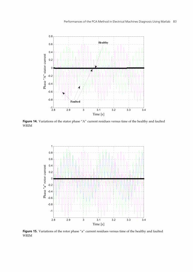
Figure 14. Variations of the stator phase “A” current residues versus time of the healthy and faulted WRIM

Figure 15. Variations of the rotor phase “a” current residues versus time of the healthy and faulted WRIM

2.8 2.9 3 3.1 3.2 3.3 3.4-1

-0.8

-0.6

-0.4

-0.2

0

0.2

0.4

0.6

0.8

Phas

e "A

" st

ator

cur

rent

Time [s]

Healthy

Faulted

2.8 2.9 3 3.1 3.2 3.3 3.4

-1

-0.8

-0.6

-0.4

-0.2

0

0.2

0.4

0.6

0.8

1

Phas

e "a

" ro

tor

curr

ent

Time [s]


Figure 16. Real variations of electromagnetic torque versus the shaft rotational speed of the WRIM

Figure 17. Variations of electromagnetic torque residues versus the shaft rotational speed residues of the WRIM

287.5 288 288.5 289 289.5 29010.3

10.35

10.4

10.45

10.5

Ele

ctro

mag

neti

c to

rque

[N

m]

Shaft rotational speed [rad/s]

40% 30% 20% 10% Healthy

-0.4 -0.3 -0.2 -0.1 0 0.1 0.2 0.3 0.4 0.5 0.6

-0.4

-0.2

0

0.2

0.4

0.6

Ele

ctro

mag

neti

c to

rque

Shaft rotational speed

Healthy

40%10%20% 30%


6. Discussion

Several types of representations are used in the signals processing domain, especially for the electrical machines diagnosis. We can mention the temporal representation (Figure 8 to Figure11, Figure 14 and Figure 15) and the signal frequency analysis. Although they have proved their efficiency, the state variable representations between them also show their advantages. They can be performed without mathematical transformation (Figure 16) and with mathematical transformation (Figure 12 and Figure 13).

The latter representation type and the temporal representation are confronted with the PCA method application results (Figure 14, Figure 15 and Figure 17). Only the simulation results with stator faults are presented because the global behavior of the state variables in both rotor and stator faults are almost similar.

For the temporal variations case, the rotor currents (Figure 9) and the shaft rotational speed (Figure 10) are the variables which produce the most information in presence of defaults. The defaults occur on the rotor current frequency and the shaft rotational speed magnitude.

The electromagnetic torque variations versus the shaft rotational speed also show clearly the WRIM operation zone in the presence of defaults (Figure 16). On the opposite, the representations with mathematical transformations (Figure 12 and Figure 13) do not provide significant information due to the fact that the stator currents remain almost unchanged in the presence of defaults (Figure 8).

With PCA method application, every representation type shows precisely the differences between healthy and faulted WRIM (Figure 14, Figure 15 and Figure 17). In the healthy case, residues are zero. When defaults appear, the residue representations have an effective value with an absolute value superior to zero.

In the figure 17, the healthy case is represented by a point situated on the coordinate origins. Therefore, one can show several right lines corresponding to the faulted cases. This behavior is due to the proportional characteristic of the considered faults.

PCA method proved to be very effective in electrical machines faults detection. This requires a good choice of the number of the principal components to be retained so that information contained in residues is relevant.

7. Implementation of the WRIM and the PCA models in the Matlab software

The differential equations system governing the WRIM is composed of linear differential equation which has the following form:

( )dy f ydt

(31)


Pre-programmed solvers are available in the Matlab software to solve easily this type of equation. These pre-programmed functions (ode45, ode113 …) proposed by the software helped to solve correctly with scalable computation time by the number of data to be processed. We adopted “ode45”, solver based on the Runge-Kutta 4, 5 numerical resolution method. After creating a function detailing the differential equation system, we have to use it in the chosen solver to calculate numerically the equations governing the WRIM.

The following extract lines of code illustrate the use of the pre-programmed function “ode45” (Figure 18):

Figure 18. Use of ode45 solver to solve the differential equations system of the WRIM

The differential equations system is established in the “Diff_Equa_WRIM” function.

One of the major strengths of Matlab is the matrix manipulation. With the amount of data in matrix form that we consider in this paper, this feature of the software allows us to treat easily and without complexity these data. Thus, for the ACP method, matrix manipulations are done by simple operations because all variables in Matlab are intrinsically represented by matrix forms. In addition, pre-programmed functions are available to perform some precise operations such as the descendant sorting with “descend” function.

And finally, Matlab offers a multitude of possibilities for graphic representations. At the end of the PCA process, the original data and those from the treatment are represented graphically. This allowed more comparative studies as well as quantitative and qualitative analysis of the entire device. A function was reserved to the automatic superposition of curves of the same variables for the different considered defaults.

To summarize, three major functions have been developed to carry out the approach:

resolution of de differential equations system governing the WRIM,


resolution of the PCA method, visualization of comparative curves.

We would like to note that each approach has been developed as a separate function, but our program runs automatically. These functions are executed automatically, one after the other, in another function.

8. Conclusion PCA method based on residues analysis has been established and applied on WRIM diagnosis.

An accurate analytical model of the machine has been proposed and simulated to perform the healthy and faulted data for PCA approach need.

Several representations of nine state variables of the machine have been analyzed. For the temporal variation without PCA, the rotor current and the shaft rotational speed are the more affected by the considered fault type. The representations of the electromagnetic torque versus the shaft rotational speed in both with and without PCA approach show clearly the presence of defaults. Indeed, PCA method is interesting for all types of representation compared to some other signal processing types.

Simulation results show the efficiency of the detection but require a good choice of the number of principal components.

Author details Jacques Fanjason Ramahaleomiarantsoa and Nicolas Héraud Université de Corse, U.M.R. CNRS 6134 SPE, BP 52, Corte, France

Eric Jean Roy Sambatra Institut Supérieur de Technologie, BP 509, Antsiranana, Madagascar

Jean Marie Razafimahenina Ecole Supérieure Polytechnique, BP O, Antsiranana, Madagascar

Acknowledgement This research was supported by MADES/SCAC Madagascar project. We are grateful for technical and financial support.

9. References [1] Benbouzid M. E. H (2000) A Review of Induction Motors Signature Analysis as a

Medium for Faults Detection, IEEE Transactions On Industrial Electronics, vol. 47, N° 5, pp. 984-993.


[2] Chia-Chou Y & al. (2008) A reconfigurable motor for experimental emulation of stator winding interturn and broken bar faults in polyphase induction machines, 01, IEEE transactions on energy conversion, vol.23, n°4. pp. 1005-1014.

[3] Sin M.L, Soong W.L, Ertugrul N (2003) Induction machine on-line condition monitoring and fault diagnosis – a survey, University of Adelaide.

[4] Negrea M.D (2006) Electromagnetic flux monitoring for detecting faults in electrical machines, PhD, Helsinki University of Technology, Department of Electrical and Communications Engineering, Laboratory of Electromechanics, TKK Dissertations 51, Espoo Finland.

[5] Liu L (2006) Robust fault detection and diagnosis for permanent magnet synchronous motors, PhD dissertation, College of Engineering, The Florida State University, USA.

[6] Benaïcha A, GuerfeL M, Bouguila N, Benothman K (2010) New PCA-based methodology for sensor fault detection and localization, 8th International Conference of Modeling and Simulation, MOSIM’10, “Evaluation and optimization of innovative production systems of goods and services”, Hammamet, Tunisia.

[7] Ku W, Storer R.H, Georgakis C (1995) Disturbance detection and isolation by dynamic principal component analysis. Chemometrics and Intelligent Laboratory Systems, 30. pp. 179-196.

[8] Huang B (2001) Process identification based on last principal component analysis, Journal of Process Control, 11. pp. 19-33.

[9] Ramahaleomiarantsoa J. F, Héraud N, Sambatra E. J. R, Razafimahenina J. M (2011) Principal Components Analysis Method Application in Electrical Machines Diagnosis, ICINCO’08, Noordwykerhout, Pays Bas.

[10] Li W, Qin S.J (2001) Consistent dynamic pca based on errors-in-variables Subspace identification, Journal of Process Control, 11(6). pp. 661-678.

[11] Valle S, Weihua L, Qin S.J (1999) Selection of the number of principal components: The variance of the reconstruction error criterion with a comparison to other methods, Industrial and Engineering Chemistry Research, vol. 38. pp. 4389-4401.

[12] Benaïcha A, Mourot G, Guerfel M, Benothman K, Ragot J (2010) A new method for determining PCA models for system diagnosis, 18th Mediterranean Conference on Control & Automation Congress Palace Hotel, Marrakech, Morocco June 23-25. pp. 862-867.

[13] Wieczorek M, Rosołowski E (2010) Modelling of induction motor for simulation of internal faults, Modern Electric Power Systems, MEPS'10, paper P29, Wroclaw, Poland.

[14] Halligan R.G, Jagannathan S (2009) PCA Based Fault isolation and prognosis with application to Water Pump, paper1, thesis, Fault detection and prediction with application to rotating machinery, Missouri University of Science and Technology.

performances of the pca method in electrical machines diagnosis

Documents