parametricsurvivalmodels -...
TRANSCRIPT
Parametric Survival Models
Christoph Dätwyler and Timon Stucki
9. May 2011

Contents
Introduction
Parametric ModelDistributional AssumptionWeibull ModelAccelerated Failure Time AssumptionA More General Form of the AFT ModelWeibull AFT ModelLog-Logistic Model
Other Parametric Models
The Parametric Likelihood
Frailty Models
Summary
Contents
Introduction
Parametric ModelDistributional AssumptionWeibull ModelAccelerated Failure Time AssumptionA More General Form of the AFT ModelWeibull AFT ModelLog-Logistic Model
Other Parametric Models
The Parametric Likelihood
Frailty Models
Summary
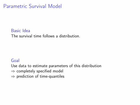
Parametric Survival Model
Basic IdeaThe survival time follows a distribution.
GoalUse data to estimate parameters of this distribution⇒ completely specified model⇒ prediction of time-quantiles

Parametric Survival Model vs. Cox PH Model
Parametric Survival Model
+ Completely specified h(t) and S(t)
+ More consistent with theoretical S(t)
+ time-quantile prediction possible– Assumption on underlying distribution
Cox PH Model
– distribution of survival time unkonwn– Less consistent with theoretical S(t) (typically step function)+ Does not rely on distributional assumptions+ Baseline hazard not necessary for estimation of hazard ratio

Contents
Introduction
Parametric ModelDistributional AssumptionWeibull ModelAccelerated Failure Time AssumptionA More General Form of the AFT ModelWeibull AFT ModelLog-Logistic Model
Other Parametric Models
The Parametric Likelihood
Frailty Models
Summary
Contents
Introduction
Parametric ModelDistributional AssumptionWeibull ModelAccelerated Failure Time AssumptionA More General Form of the AFT ModelWeibull AFT ModelLog-Logistic Model
Other Parametric Models
The Parametric Likelihood
Frailty Models
Summary

Probability Density, Hazard and Survival Function
Main AssumptionThe survival time T is assumed to follow a distribution with densityfunction f (t).
⇒ S(t) = P(T > t) =
∫ ∞t
f (u)du
Recall:
h(t) = −ddt S(t)
S(t), S(t) = exp
(−∫ t
0h(u)du
)
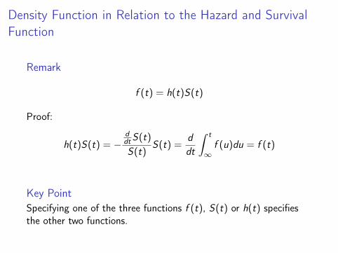
Density Function in Relation to the Hazard and SurvivalFunction
Remark
f (t) = h(t)S(t)
Proof:
h(t)S(t) = −ddt S(t)
S(t)S(t) =
ddt
∫ t
∞f (u)du = f (t)
Key PointSpecifying one of the three functions f (t), S(t) or h(t) specifiesthe other two functions.

Commonly Used Distributions and Parameters
Distribution f (t) S(t) h(t)
Exponential λ exp(−λt) exp(−λt) λWeibull λptp−1 exp(−λtp) exp(−λtp) λptp−1
Log-logistic λptp−1
(1+λtp)21
1+λtpλptp−1
1+λtp
Modeling of the parameters:I λ is reparameterized in terms of predictor variables and
regression parameters.I Typically for parametric models, the shape parameters p is
held fixed.

Contents
Introduction
Parametric ModelDistributional AssumptionWeibull ModelAccelerated Failure Time AssumptionA More General Form of the AFT ModelWeibull AFT ModelLog-Logistic Model
Other Parametric Models
The Parametric Likelihood
Frailty Models
Summary

Weibull ModelAssuming T ∼Weibull(λ, p) with probability density function
f (t) = λptp−1 exp(−λtp), where p > 0 and λ > 0,
the hazard function is given by
h(t) = λptp−1.
p is called shape parameter:
I If p > 1 the hazard increases
I If p = 1 the hazard is constant(exponential model)
I If p < 1 the hazard decreases
0 2 4 6 8 10
0.5
1.0
1.5
t
h(t)
p<1p=1p>1
Hazard Function h(t)

Graphical Evaluation of Weibull Assumption
Property of Weibull ModelThe log(− log(S(t))) is linear with the log of time.
S(t) = exp(−λtp)
⇒ − log(S(t)) = λtp
⇒ log(− log(S(t))) = log(λ) + p log(t)
This property allows a graphical evaluation of the appropriatenessof a Weibull model by plotting
log(− log(S(t))) vs. log(t),
where S(t) is Kaplan-Meier survival estimate.

Example: Remission DataWe consider the remission data of 42 leukemia patients.
I 21 patients given treatment (TRT = 1)I 21 patients given placebo (TRT = 0)
Note: The survival time (time to event) is the time until a patientwent out of remission, which means that the patient relapsed.
●
●
●
●
●
●
●
●
●
●
●
0.0 0.5 1.0 1.5 2.0 2.5 3.0
−2.
0−
1.5
−1.
0−
0.5
0.0
0.5
1.0
log(t)
log(
−lo
g(S
(t)))
● TRT = 0TRT = 1
I straight lines ⇒ WeibullI same slope ⇒ PH

Weibull PH Model
Recall: h(t) = λptp−1
Weibull PH model:I Reparameterize λ with
λ = exp(β0 + β1TRT ).
I Then the hazard ratio (TRT = 1 vs. TRT = 0) is
HR =exp(β0 + β1)ptp−1
exp(β0)ptp−1 = exp(β1),
which indicates that the PH assumption is satisfied.
Note: This result depends on p having the same value for TRT = 1and TRT = 0 (otherwise time would not cancel out).

Exponential PH Model
The exponential distribution is a special case of the Weibulldistribution with p = 1.
Weibull density function:
f (t) = exp(−λtp)︸ ︷︷ ︸S(t)
λptp−1︸ ︷︷ ︸h(t)
Setting p = 1 gives the density function of an exponentialdistribution
f (t) = exp(−λt)︸ ︷︷ ︸S(t)
λ︸︷︷︸h(t)
.

Exponential PH Model
Running the exponential model leads to the following output:
264 7. Parametric Survival Models
h(t) = λ = exp(β0 + β1TRT)
TRT = 1: h(t) = exp(β0 + β1)TRT = 0: h(t) = exp(β0)
HR(TRT = 1 vs. TRT = 0)
= exp(β0 + β1)exp(β0)
= exp(β1)
For simplicity, we demonstrate an exponentialmodel that has TRT as the only predictor. Westate the model in terms of the hazard by repa-rameterizing λ as exp(β0 + β1TRT). With thismodel, the hazard for subjects in the treated groupis exp(β0 + β1) and the hazard for the placebogroup is exp(β0). The hazard ratio comparing thetreatment and placebo (see left side) is the ratio ofthe hazards exp(β1). The exponential model is aproportional hazards model.
Constant Hazards⇒ Proportional Hazards
Proportional Hazards⇒\ Constant Hazards
Exponential Model—Hazards areconstant
Cox PH Model—Hazards are pro-portional not necessarily constant
The assumption that the hazard is constant foreach pattern of covariates is a much stronger as-sumption than the PH assumption. If the hazardsare constant, then of course the ratio of the haz-ards is constant. However, the hazard ratio beingconstant does not necessarily mean that eachhazard is constant. In a Cox PH model the base-line hazard is not assumed constant. In fact, theform of the baseline hazard is not even specified.
Remission Data
Exponential regressionlog relative-hazard form
t Coef. Std. Err. z p >|z|trt −1.527 .398 −3.83 0.00cons −2.159 .218 −9.90 0.00
Output from running the exponential model isshown on the left. The model was run using Statasoftware (version 7.0). The parameter estimatesare listed under the column called Coef. The pa-rameter estimate for the coefficient of TRT (β1) is−1.527. The estimate of the intercept (called consin the output) is −2.159. The standard errors (Std.Err.), Wald test statistics (z), and p-values for theWald test are also provided. The output indicatesthat the z test statistic for TRT is statistically sig-nificant with a p-value <0.005 (rounds to 0.00 inthe output).
Coefficient estimates obtained by MLE↘asymptotically normal
The regression coefficients are estimated usingmaximum likelihood estimation (MLE), andare asymptotically normally distributed.
The estimated hazard ratio is obtained from the estimatedcoefficient β1 by
HR(TRT = 1 vs. TRT = 0) = exp(β1) = exp(−1.527) = 0.22.
InterpretationThis means that the hazard for the group with TRT = 0 is biggerthan the one for the group with TRT = 1 because 0.22 < 1,indicating a positive effect of the treatment.

Contents
Introduction
Parametric ModelDistributional AssumptionWeibull ModelAccelerated Failure Time AssumptionA More General Form of the AFT ModelWeibull AFT ModelLog-Logistic Model
Other Parametric Models
The Parametric Likelihood
Frailty Models
Summary

Accelerated Failure Time Assumption
First example: Humans vs. dogsI Let SH(t) and SD(t) denote the survival functions for humans
and dogs respectively.I Known: In general dogs grow older seven times faster than
humans.I In AFT terminology: The probability of a dog surviving past t
years is equal to the one of a human surviving past 7t years.I This means:
SD(t) = SH(7t)
I In other words, dogs accelerate through life about seven timesfaster than humans.
AFT Models
AFT ModelsAFT Models describe stretching out or contraction of survival timeas a function of predictor variables.

Illustration of AFT Assumption
Second example: Smokers vs. nonsmokersI Let SS(t) and SNS(t) denote the survival functions for
smokers and nonsmokers respectively.
AFT assumption
SNS(t) = SS(γt) for t ≥ 0
Definitionγ > 0 is the so called acceleration factor and is a constant.

Expressing the AFT assumption
The AFT assumption can be expressedI in terms of survival function as seen before:
SNS(t) = SS(γt)
I in terms of random variables for survival time:
γTNS = TS ,
where TNS is a random variable following some distributionrepresenting the survival time for nonsmokers and TS theanalogous one for smokers.

Acceleration factor
The acceleration factor allows to evaluate the effect of predictorvariables on the survival time.
Acceleration factorThe acceleration factor is a ratio of time-quantiles corresponding toany fixed value of S(t).268 7. Parametric Survival Models
1.00
0.75
0.50
0.25
S(t)
G = 1 G = 2t
γ = 2
distance to G = 1
distance to G = 2
Survival curves for Group 1 (G = 1)and Group 2 (G = 2)
Horizontal lines are twice as long toG = 2 compared to G = 1 becauseγ = 2
This idea is graphically illustrated by examiningthe survival curves for Group 1 (G = 1) and Group2 (G = 2) shown on the left. For any fixed value ofS(t), the distance of the horizontal line from theS(t) axis to the survival curve for G = 2 is doublethe distance to the survival curve for G = 1. No-tice the median survival time (as well as the 25thand 75th percentiles) is double for G = 2. For AFTmodels, this ratio of survival times is assumed con-stant for all fixed values of S(t).
V. Exponential ExampleRevisited
Remission data (n = 42)
21 patients given treatment (TRT = 1)21 patients given placebo (TRT = 0)
Previously discussed PH form ofmodelNow discuss AFT form of model
We return to the exponential example applied tothe remission data with treatment status (TRT) asthe only predictor. In Section III, results from thePH form of the exponential model were discussed.In this section we discuss the AFT form of themodel.
Exponential survival and hazardfunctions:
S(t) = exp(−λt)h(t) = λ
Recall for PH model:
h(t) = λ = exp(β0 + β1 TRT)
The exponential survival and hazard functions areshown on the left. Recall that the exponential haz-ard is constant and can be reparameterized as aPH model, h(t) = λ = exp(β0 + β1TRT). In thissection we show how S(t) can be reparameterizedas an AFT model.

Interpretation of the Acceleration Factor
Assuming the event to occur is negative for an individual,comparing two groups (levels of covariates) leads to the followinggeneral interpretation:
γ > 1 ⇒ exposure benefits survivalγ < 1 ⇒ exposure harmful to survival
For the hazard ratio, we have:
HR > 1 ⇒ exposure harmful to survivalHR < 1 ⇒ exposure benefits survival
γ = HR = 1 ⇒ no effect from exposure

Contents
Introduction
Parametric ModelDistributional AssumptionWeibull ModelAccelerated Failure Time AssumptionA More General Form of the AFT ModelWeibull AFT ModelLog-Logistic Model
Other Parametric Models
The Parametric Likelihood
Frailty Models
Summary

General Form of AFT Model
Consider an AFT model with one predictor X . The model can beexpressed on the log scale as
log(T ) = α0 + α1X + ε,
where ε is a random error following some distribution.
T log(T )Exponential Extreme valueWeibull Extreme valueLog-logistic LogisticLognormal Normal
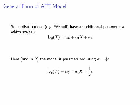
General Form of AFT Model
Some distributions (e.g. Weibull) have an additional parameter σ,which scales ε.
log(T ) = α0 + α1X + σε
Here (and in R) the model is parametrized using σ = 1p :
log(T ) = α0 + α1X +1pε
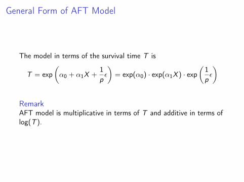
General Form of AFT Model
The model in terms of the survival time T is
T = exp(α0 + α1X +
1pε
)= exp(α0) · exp(α1X ) · exp
(1pε
)
RemarkAFT model is multiplicative in terms of T and additive in terms oflog(T ).

Contents
Introduction
Parametric ModelDistributional AssumptionWeibull ModelAccelerated Failure Time AssumptionA More General Form of the AFT ModelWeibull AFT ModelLog-Logistic Model
Other Parametric Models
The Parametric Likelihood
Frailty Models
Summary

AFT Model
I We use again the remission data.I We consider the variable TRT as only predictor (TRT = 1
and TRT = 0)
AFT Model AssumptionThe ratio of time-quantile is constant (γ) for all fixed valuesS(t) = q.
Expression for time-quantiles
I Solve for t in terms of S(t)
I Scale t in terms of predictors

Weibull AFT ModelRecall: S(t) = exp(−λtp)
1. Solving for t gives:
S(t) = exp(−λtp)⇔ − log(S(t)) = λtp
⇔ t = (− log(S(t)))1/p 1λ1/p
2. Reparameterizing 1λ1/p = exp(α0 + α1TRT ) yields
t = (− log(S(t)))1/p exp(α0 + α1TRT ).
(TRT used to scale time to any fixed value of S(t))
3. In terms of any fixed probability S(t) = q we get
t = (− log(q))1/p exp(α0 + α1TRT ).

Weibull AFT Model: Acceleration Factor
The acceleration factor for a fixed value of S(t) = q is calculatedas follows:
Level of covariates: TRT = 1 and TRT = 0
Then the acceleration factor γ is
γ = γ(TRT = 1 vs. TRT = 0)
=(− log(q))1/p exp(α0 + α1)
(− log(q))1/p exp(α0)
= exp(α1).
Note: As in the PH form of the model, this result depends on phaving the same value for TRT = 1 and TRT = 0.

R Code and R Output
> weibull.aft <- survreg(Surv(Survt,status) ~ TRT,dist=’weibull’)> summary(weibull.aft)
Call:survreg(formula = Surv(Survt, status) ~ TRT, dist = "weibull")
Value Std. Error z p(Intercept) 2.248 0.166 13.55 8.30e-42TRT 1.267 0.311 4.08 4.51e-05Log(scale) -0.312 0.147 -2.12 3.43e-02
Scale= 0.732
Weibull distributionLoglik(model)= -106.6 Loglik(intercept only)= -116.4
Chisq= 19.65 on 1 degrees of freedom, p= 9.3e-06Number of Newton-Raphson Iterations: 5n= 42

R Code and R Output: Acceleration Factor
The estimated acceleration factor γ comparing the treatment groupto the placebo group (TRT = 1 vs. TRT = 0) is now:
γ = exp(α1)
> exp(weibull.aft$coefficient[2])TRT
3.551374
InterpretationThe survival time for the treatment group (TRT = 1) is increasedby a factor of 3.55 compared to the placebo group (TRT = 0)⇒ Treatment is positive.
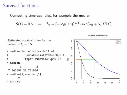
Survival functions
Computing time-quantiles, for example the median:
S(t) = 0.5 ⇒ tm = (− log(0.5))1/p · exp(α0 + α1TRT )
Estimated survival times for themedian S(t) = 0.5:
> median <-predict(weibull.aft,+ newdata=list(TRT=c(0,1)),+ type=’quantile’,p=0.5)> median
1 27.242697 25.721526
> median[2]/median[1]2
3.551374 0 10 20 30 40 50 60
0.0
0.2
0.4
0.6
0.8
1.0
t
S(t
)
TRT=0TRT=1
Survival Function S(t)

Relation between Weibull AFT and PH coefficients
I AFT: 1λ1/p = exp(α0 + α1TRT )
⇔ (1/p) log(λ) = −(α0 + α1TRT )⇔ log(λ) = −p(α0 + α1TRT )
I PH: λ = exp(β0 + β1TRT )⇔ log(λ) = β0 + β1TRT
This indicates the following relationship between the coefficients:
βj = −αjp

Exponential PH and AFT Model
We obtained βj = −αjp for the Weibull model. In the special caseof the exponential model where p = 1 we have
βj = −αj .
RemarkThe exponential PH and AFT are in fact the same model, exceptthat the parametrization is different.

Exponential PH and AFT Model
Example:The estimated values from the exponential example above supportthis result.
Coefficient PH Model: β1 = −1.527Coefficient AFT Model: α1 = 1.527
We also have
HR(TRT = 1vs. TRT = 0) = exp(β1) = exp(−α1) =1γ.

Property of the Weibull Model
PropositionAFT assumption holds ⇔ PH assumption holds (given that p isfixed)
Proof for the considered example (TRT = 1 and TRT = 0):
I [⇒]: γ = exp(α1)Assume γ is constant ⇒ α1 is constantHR = exp(β1) = exp(−pα1) ⇒ HR is constant
I [⇐]: HR = exp(β1)Assume HR is constant ⇒ β1 is constantγ = exp(α1) = exp(−β1
p ) ⇒ γ is constant

Possible Plots
Possible results for plots of log(− log(S(t))) against log(t):
⇒ Weibull (or Exponential if p = 1), PH andAFT assumption hold.
⇒ Not Weibull, PH and not AFT.
⇒ Not Weibull, not PH and not AFT.
⇒ Weibull, not PH and not AFT (p not fixed).

Contents
Introduction
Parametric ModelDistributional AssumptionWeibull ModelAccelerated Failure Time AssumptionA More General Form of the AFT ModelWeibull AFT ModelLog-Logistic Model
Other Parametric Models
The Parametric Likelihood
Frailty Models
Summary

Hazard Function of Log-Logistic ModelThe log-logistic distribution accommodates an AFT model but nota PH model.Hazard function is
h(t) =λptp−1
1 + λtp ,
with p > 0 and λ > 0.
Shape of hazard function:I p ≤ 1: hazard decreasesI p > 1: hazard unimodal
0 1 2 3 4 5
0.2
0.4
0.6
0.8
1.0
t
h(t)
p<=1p>1
Hazard Function h(t)

PO Assumption
DefinitionIn a proportional odds (PO) survival model, the odds ratio isconstant over time.
I Survival odds: odds of surviving beyond time t
S(t)
1− S(t)=
P(T > t)
P(T ≤ t)
I Failure odds: odds of getting the event by time t
1− S(t)
S(t)=
P(T ≤ t)
P(T > t)

PO Assumption
The failure odds of the log-logistic survival model are
1− S(t)
S(t)=
λtp1+λtp
11+λtp
= λtp.
The failure odds ratio (OR) for two different groups (1 and 2) is(for p fixed)
OR(1 vs. 2) =
1−S1(t)S1(t)
1−S2(t)S2(t)
=λ1tp
λ2tp =λ1
λ2.
Hence, the log-logistic model is a proportional odds (PO) model.
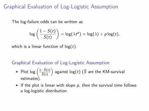
Graphical Evaluation of Log-Logistic Assumption
The log-failure odds can be written as
log(1− S(t)
S(t)
)= log(λtp) = log(λ) + p log(t),
which is a linear function of log(t).
Graphical Evaluation of Log-Logistic Assumption
I Plot log(
1−S(t)S(t)
)against log(t) (S are the KM-survival
estimates).I If the plot is linear with slope p, then the survival time follows
a log-logistic distribution.

Log-Logistic Example with the Remission DataWe consider a new categorical variable WBCCAT :
I WBCCAT = 2 if logWBC ≥ 2.5 (high count)I WBCCAT = 1 if logWBC < 2.5 (medium count)
The graphical evaluation of WBCCAT = 2 and WBCCAT = 1:
●
●
●
●
●
● ● ●●
●
●● ●●●
0.0 0.5 1.0 1.5 2.0 2.5 3.0 3.5
−2
−1
01
23
log(t)
log(
(1−
S(t)
)S
(t))
● WBCCAT=1WBCCAT=2
Log Failure Odds vs. Log Time
⇒ straight lines indicatelog-logistic distribution

AFT Log-Logistic Model
AFT log-logistic model with WBCCAT as only predictor:
We solveS(t) =
11 + λtp =
1
1 + (λ1p t)p
for t and obtain
t =
(1
S(t)− 1) 1
p 1
λ1p.
We reparameterize the factor on the right as
1
λ1p
= exp(α0 + α1WBCCAT ).

AFT Log-Logistic Model: Acceleration Factor
We get
t =
(1
S(t)− 1) 1
p
exp(α0 + α1WBCCAT ).
For a fixed probability S(t) = q, the expression for t is
t =(q−1 − 1
) 1p exp(α0 + α1WBCCAT ).
The acceleration factor γ for S(t) = q is
γ(WBCCAT = 2 vs. WBCCAT = 1) =
(q−1 − 1
) 1p exp(α0 + 2α1)
(q−1 − 1)1p exp(α0 + 1α1)
= exp(α1).

R Code and R Output
> logistic.aft <- survreg(Surv(Survt, status) ~ WBCCAT,+ dist=’loglogistic’,data=remdata)> summary(logistic.aft)
Call:survreg(formula = Surv(Survt, status) ~ WBCCAT, data = remdata,
dist = "loglogistic")Value Std. Error z p
(Intercept) 4.094 0.586 6.98 2.92e-12WBCCAT -0.987 0.337 -2.93 3.40e-03Log(scale) -0.564 0.154 -3.67 2.41e-04
Scale= 0.569
Log logistic distributionLoglik(model)= -111.2 Loglik(intercept only)= -115.4
Chisq= 8.28 on 1 degrees of freedom, p= 0.004Number of Newton-Raphson Iterations: 4n= 42

R Code and R Output: Acceleration Factor
The estimated acceleration factor γ comparing WBCCAT = 2(high count) and WBCCAT = 1 (medium count) is now:
γ = exp(α1)> exp(logistic.aft$coefficient[2])
WBCCAT0.3728214
⇒ S1(t) = S2(0.37t)
(Si is the survival function for WBCCAT = i , i = 1,2)
InterpretationThe survival time for the group with high count (WBCCAT = 2) is"accelerated" by a factor of 0.37 compared to the group withmedium count (WBCCAT = 1) ⇒ High WBC is negative.

PO Log-Logistic Model
The proportional odds (PO) form of the log-logistic model can beformulated by reparameterizing λ.
Failure odds:1− S(t)
S(t)=
λtp1+λtp
11+λtp
= λtp.
Reparameterizing λ gives
λ = exp(β0 + β1WBCCAT ).
Hence, the failure odds ratio is
OR(WBCCAT=2 vs. WBCCAT=1) =tp exp(β0 + 2β1)
tp exp(β0 + 1β1)= exp(β1).

Comparing AFT and PO Log-Logistic Model
Parameterizations:I AFT model: 1
λ1p
= exp(α0 + α1WBCCAT )
I PO model: λ = exp(β0 + β1WBCCAT )
Hence, we have the relationship
β0 = −α0p and β1 = −α1p.
Note: If p is fixed this leads to: AFT ⇔ PO
So we can calculate the estimated OR with the coefficients of theAFT model by:
OR = exp(β1)
= exp(−α1p) = 5.66
> alpha1 <- logistic.aft$coefficient[2]> p <- 1/logistic.aft$scale> exp(-alpha1*p)5.662691

Graphical Evaluation
●
●
●
●
●
● ● ●●
●
●● ●●●
0.0 0.5 1.0 1.5 2.0 2.5 3.0 3.5
−2
−1
01
23
log(t)
log(
(1−
S(t)
)S
(t))
● WBCCAT=1WBCCAT=2
Log Failure Odds vs. Log Time

Graphical Evaluation
Proposition
1. Straight lines ⇒ Log-logistic2. Parallel plots and log-logistic ⇒ PO3. Log-logistic and PO ⇒ AFT
Proof: Consider two groups (1 and 2).1. log(failure odds) = log(λ) + p log(t)
2. Parallel plots ⇒ p the same for both groups⇒ OR = tpλ1
tpλ2= λ1
λ2
3. For S(t) = q, the acceleration factor is
γ =
(q−1 − 1
) 1p λ1
(q−1 − 1)1p λ2
=λ1
λ2.

Contents
Introduction
Parametric ModelDistributional AssumptionWeibull ModelAccelerated Failure Time AssumptionA More General Form of the AFT ModelWeibull AFT ModelLog-Logistic Model
Other Parametric Models
The Parametric Likelihood
Frailty Models
Summary

Generalized Gamma Model
The generalized gamma distribution is given by
f (t) =pad td−1 exp(−( t
a)p)
Γ(d/p),
whereΓ(z) =
∫ ∞0
sz−1e−sds
and a > 0, d > 0, p > 0.
I The three parameters allow great flexibility in the distributionsshape.
I Weibull and lognormal distributions are special cases of thegeneralized gamma distribution (e.g. setting d = p gives usthe Weibull distribution).

Lognormal Model
The lognormal distribution is given by
f (t) =1
tσ√2π
exp(−(log(t)− µ)2
2σ2
),
where µ and σ are the mean and standard deviation respectively, ofthe variable’s natural logarithm (by definition, the variable’slogarithm is normally distributed).
I Shape similar to the log-logistic distribution (and yields similarmodel results)
I Accommodates an AFT model (as the log-logistic), but is nota proportional odds model (whereas the log-logistic model is aPO model)
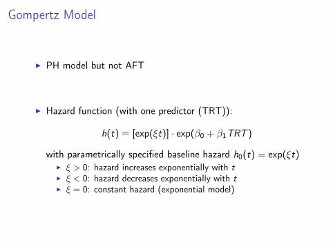
Gompertz Model
I PH model but not AFT
I Hazard function (with one predictor (TRT)):
h(t) = [exp(ξt)] · exp(β0 + β1TRT )
with parametrically specified baseline hazard h0(t) = exp(ξt)I ξ > 0: hazard increases exponentially with tI ξ < 0: hazard decreases exponentially with tI ξ = 0: constant hazard (exponential model)

Modeling the Shape Parameter
Many parametric models contain a shape parameter, which isusually considered fixed.
Example:
I Weibull modelRecall: h(t) = λptp−1 where λ = exp(β0 + β1TRT ) and p,the shape parameter, unaffected by predictors.
I Alternative Weibull modelNow: h(t) = λptp−1 where λ = exp(β0 + β1TRT ) andp = exp(δ0 + δ1TRT )
I If δ1 6= 0, the value of p differs by TRTI Not a PH or AFT model if δ1 6= 0, but still a Weibull model

Contents
Introduction
Parametric ModelDistributional AssumptionWeibull ModelAccelerated Failure Time AssumptionA More General Form of the AFT ModelWeibull AFT ModelLog-Logistic Model
Other Parametric Models
The Parametric Likelihood
Frailty Models
Summary

Parametric Likelihood and Censoring
The likelihood function for a parametric modelI is a function of the observed data and the unknown
parameters of the model.I is based on the distribution of the survival time.I depends on the censoring of the data.
286 7. Parametric Survival Models
Alternative Weibull modelmodels the ancillary parameter p
h(t) = λpt p−1
where λ = exp(β0 + β1TRT)p = exp(δ0 + δ1TRT)
Not a PH or AFT model if δ1 �= 0but still a Weibull model
An alternative approach is to model the shape pa-rameter in terms of predictor variables and regres-sion coefficients. In the Weibull model shown onthe left, both λ and p are modeled as functions oftreatment status (TRT). If δ1 is not equal to zero,then the value of p differs by TRT. For that sit-uation, the PH (and thus the AFT) assumption isviolated because t p−1 will not cancel in the hazardratio for TRT (see Practice Exercises 15 to 17).
Choosing appropriate model� Evaluate graphically◦ Exponential◦ Weibull◦ Log-logistic� Akaike’s information criterion◦ Compares model fit◦ Uses −2 log likelihood
Choosing the most appropriate parametric modelcan be difficult. We have provided graphical ap-proaches for evaluating the appropriateness ofthe exponential, Weibull, and log-logistic models.Akaike’s information criterion (AIC) providesan approach for comparing the fit of models withdifferent underlying distributions, making use ofthe −2 log likelihood statistic (described in Prac-tice Exercises 11 and 14).
X. The Parametric Likelihood� Function of observed data andunknown parameters� Based on outcome distributionf(t)� Censoring complicates survivaldata◦ Right-censored◦ Left-censored◦ Interval-censored
The likelihood for any parametric model is a func-tion of the observed data and the model’s un-known parameters. The form of the likelihoodis based on the probability density function f(t)of the outcome variable. A complication of sur-vival data is the possible inclusion of censoredobservations (i.e., observations in which the ex-act time of the outcome is unobserved). We con-sider three types of censored observations: right-censored, left-censored, and interval-censored.
Examples of Censored Subjects
Right-censored:10
10
108
Left-censored: __________________ time
Interval-censored: ______________ time
x
x
x
time
Right-censored. Suppose a subject is lost tofollow-up after 10 years of observation. The timeof event is not observed because it happened af-ter the 10th year. This subject is right-censored at10 years because the event happened to the rightof 10 on the time line (i.e., t > 10).
Left-censored. Suppose a subject had an event be-fore the 10th year but the exact time of the event isunknown. This subject is left-censored at 10 years(i.e., t < 10).
Interval-censored. Suppose a subject had anevent between the 8th and 10th year (exact timeunknown). This subject is interval-censored (i.e.,8 < t < 10).
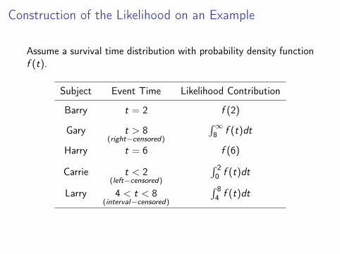
Construction of the Likelihood on an Example
Assume a survival time distribution with probability density functionf (t).
Subject Event Time Likelihood Contribution
Barry t = 2 f (2)
Gary t > 8(right−censored)
∫∞8 f (t)dt
Harry t = 6 f (6)
Carrie t < 2(left−censored)
∫ 20 f (t)dt
Larry 4 < t < 8(interval−censored)
∫ 84 f (t)dt

Construction of the Likelihood on an Example
The likelihood function L is the product of each contribution:
L = f (2) ·∫ ∞
8f (t)dt · f (6) ·
∫ 2
0f (t)dt ·
∫ 8
4f (t)dt
Assumptions for formulating L:I Subjects are independent (product of contributions).I No competing risks:
No competing event prohibits a subject from eventuallygetting the event of interest.Example: Death
I Follow-up times are continuous without gaps(i.e. subjects do not return into study).
Maximum likelihood Estimates
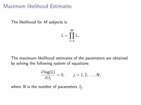
The likelihood for M subjects is
L =M∏i=1
Li .
The maximum likelihood estimates of the parameters are obtainedby solving the following system of equations
∂ log(L)
∂βj= 0, j = 1, 2, . . . ,N,
where N is the number of parameters βj .
Parametric and Cox likelihood
In a parametric model, the parametric likelihood handles easilyright-, left- or interval-censored data.In a Cox model, the Cox likelihood handles right-censored data, butis not designed to accommodate left- or interval-censored datadirectly.Example:
I Health check for nonsymptomatic outcome every year onceI If event was detected e.g. at the beginning of the third year,
the exact time when the event occurred was between thesecond and third year
I Fit a parametric model with the distribution of the outcomedenoted by f (t)
I Each subject’s contribution to the likelihood is obtained byintegrating f (t) over the interval in which it had the event.

Contents
Introduction
Parametric ModelDistributional AssumptionWeibull ModelAccelerated Failure Time AssumptionA More General Form of the AFT ModelWeibull AFT ModelLog-Logistic Model
Other Parametric Models
The Parametric Likelihood
Frailty Models
Summary

Frailty
What is frailty?I Random componentI Accounts for variability due to unobserved individual-level
factors (unaccounted for by the other predictors)
The frailty α (α > 0)I is an unobserved multiplicative effect on the hazardI follows some distribution g(α) with the mean of g(α) equal to
1 (µ = 1)I θ = Var(g(α)), parameter to be estimated from the data

Hazard functions, Survival functions and Frailty
Express an individual’s hazard function conditional on the frailty as
h(t | α) = αh(t)
This leads to:
S(t | α) = exp[−∫ t
0h(u | α)du
]= exp
[−∫ t
0αh(u)du
]= exp
[−∫ t
0h(u)du
]α= S(t)α
Suppose α > 1. Then we get:I Increased hazardI Decreased survival
And vice versa for α < 1.

Survival functions in Frailty ModelsDistinguish between
I the individual level or conditional survival functionS(t | α)
I and the population level or unconditional survival functionSU(t), representing a population average.
Once the frailty distribution g(α) is chosen we find theunconditional survival function by
SU(t) =
∫ ∞0
S(t | α)g(α)dα
Then we can find the corresponding unconditional hazard hU(t)using the known relationship between survival and hazard function
hU(t) =−d [SU(t)]/dt
SU(t)

Example: Weibull PH model with and without frailty
296 7. Parametric Survival Models
Frailty distribution g(α), α > 0,E(α) = 1
Stata offers choices for g(α)1. Gamma2. Inverse-GaussianBoth distributions parameterized interms of θ
Any distribution for α > 0 with a mean of 1can theoretically be used for the distribution ofthe frailty. Stata supports two distributions: thegamma distribution and the inverse-Gaussiandistribution for the frailty. With the mean fixedat 1, both these distributions are parameterized interms of the variance θ and typically yield similarresults.
EXAMPLE
Vet Lung Cancer Trial
Predictors:
TX (dichotomous: 1 = standard, 2 = test)
PERF (continuous: 0 = worst, 100 = best)
DD (disease duration in months)
AGE (in years)
PRIORTX (dichotomous: 0 = none,10 = some)
To illustrate the use of a frailty model, we applythe data from the Veteran’s Administration LungCancer Trial described in Chapter 5. The exposureof interest is treatment status TX (standard = 1,test = 2). The control variables are performancestatus (PERF), disease duration (DD), AGE, andprior therapy (PRIORTX), whose coding is shownon the left. The outcome is time to death (in days).
Model 1. No Frailty
Weibull regression (PH form)
Log likelihood = −206.20418
t Coef. Std. Err. z p >|z|tx .137 .181 0.76 0.450perf −.034 .005 −6.43 0.000dd .003 .007 0.32 0.746age −.001 .009 −0.09 0.927priortx −.013 .022 −0.57 0.566cons −2.758 .742 −3.72 0.000
/ln p −.018 .065 −0.27 0.786
p .982 .0641/p 1.02 .066
Output from running a Weibull PH model with-out frailty using Stata software is shown on theleft (Model 1). The model can be expressed: h(t) =λpt p−1 where
λ = exp(β0 + β1TX + β2PERF + β3DD+ β4AGE + β5PRIORTX).
The estimate of the hazard ratio comparing TX = 2vs. TX = 1 is exp(0.137) = 1.15 controlling for per-formance status, disease duration, age, and priortherapy. The estimate for the shape parameter is0.982 suggesting a slightly decreasing hazard overtime.
Model 1:h(t) = λptp−1 where
λ = exp(β0 + β1TX + β2PERF + β3DD+ β4AGE + β5PRIORTX )
Example: Weibull PH model with and without frailtyPresentation: XII. Frailty Models 297
EXAMPLE (continued)
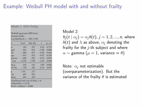
Model 2. With Frailty
Weibull regression (PH form)Gamma frailtyLog likelihood = −200.11338
t Coef. Std. Err. z p >|z|tx .105 .291 0.36 0.719perf −.061 .012 −5.00 0.000dd −.006 .017 −0.44 0.663age −.013 .015 −0.87 0.385priortx −.006 .035 −0.18 0.859cons −2.256 1.100 −2.05 0.040
/ln p .435 .141 3.09 0.002/ln the −.150 .382 −0.39 0.695
p 1.54 .2171/p .647 .091theta .861 .329
Likelihood ratio test of theta = 0:chibar2(01) = 12.18Prob>=chibar2 = 0.000
Model 2 (output on left) is the same Weibull modelas Model 1 except that a frailty component hasbeen included. The frailty in Model 2 is assumedto follow a gamma distribution with mean 1 andvariance equal to theta (θ ). The estimate of thetais 0.861 (bottom row of output). A variance ofzero (theta = 0) would indicate that the frailtycomponent does not contribute to the model. Alikelihood ratio test for the hypothesis theta = 0is shown directly below the parameter estimatesand indicates a chi-square value of 12.18 with 1degree of freedom yielding a highly significantp-value of 0.000 (rounded to 3 decimals).
Notice how all the parameter estimatesare altered with the inclusion of the frailty.The estimate for the shape parameter is now 1.54,quite different from the estimate 0.982 obtainedfrom Model 1. The inclusion of frailty not onlyhas an impact on the parameter estimates butalso complicates their interpretation.
Comparing Model 2 with Model 1� There is one additionalparameter to estimate inModel 2� The actual values ofindividuals’ frailty are notestimated in Model 2� The coefficients for thepredictor variables in Models 1and 2 have different estimatesand interpretation� The estimate of the shapeparameter is <1.0 for Model 1and >1.0 for Model 2
Before discussing in detail how the inclusionof frailty influences the interpretation of theparameters, we overview some of the key points(listed on the left) that differentiate Model 2(containing the frailty) and Model 1.
Model 2 contains one additional parameter,the variance of the frailty. However, the actualvalues of each subject’s frailty are not estimated.The regression coefficients and Weibull shapeparameter also differ in their interpretations forModel 2 compared to Model 1. We now elaborateon these points.
Model 2:hj(t | αj) = αjh(t), j = 1, 2, ..., n, whereh(t) and λ as above, αj denoting thefrailty for the j-th subject and whereα ∼ gamma (µ = 1, variance = θ)
Note: αj not estimable(overparameterization). But thevariance of the frailty θ is estimated

Example: Weibull PH model with and without frailty
For Model 1 we get HR = exp(0.137) = 1.15.For Model 2 we get HR = exp(0.105) = 1.11.
RemarkIn Model 2 the value we obtained is the estimated hazard ratio fortwo individuals having the same frailty one taking the test and theother taking the standard treatment (and same levels of otherpredictors).
Example: Weibull PH model with and without frailty
Compare the estimated values for the shape parameter p:I Model 1: p = 0.982 (→ decreasing hazard)I Model 2: p = 1.54 (→ increasing individual level hazard)
BUT: For frailty models one has to distinguish between theindividual level and population level hazard.
I Individual level/conditional hazard is estimated to increaseI Population level/unconditional hazard has an unimodal shape
(first increasing, then decreasing to 0)

Conditional and Unconditional Hazards in Frailty Models
300 7. Parametric Survival Models
Estimated unconditional hazardModel 2 (TX = 1, mean level forother covariates, p = 1.54)
analysis time
Weibull regression
tx =
1H
azar
d f
un
ctio
n
1
On the left is a plot (from Model 2) of theestimated unconditional hazard for those on stan-dard treatment (TX = 1) with mean values forthe other covariates. The graph is unimodal, withthe hazard first increasing and then decreasingover time. So each individual has an estimatedincreasing hazard ( p = 1.54), yet the hazardaveraged over the population is unimodal, ratherthan increasing. How can this be?
The answer is that the population is com-prised of individuals with different levels offrailty. The more frail individuals (α > 1) havea greater hazard and are more likely to get theevent earlier. Consequently, over time, the “at riskgroup” has an increasing proportion of less frailindividuals (α < 1), decreasing the populationaverage, or unconditional, hazard.
Four increasing individual levelhazards, but average hazard de-creases from t1 to t2
h(t)
h1
x
x
x
xh2
t1 t2
average hazard: h2 < h1
To clarify the above explanation, consider thegraph on the left in which the hazards for fourindividuals increase linearly over time until theirevent occurs. The two individuals with the high-est hazards failed between times t1 and t2 and theother two failed after t2. Consequently, the aver-age hazard (h2) of the two individuals still at riskat t2 is less than the average hazard (h1) of the fourindividuals at risk at t1. Thus the average hazardof the “at risk” population decreased from t1 tot2 (i.e., h2 < h1) because the individuals survivingpast t2 were less frail than the two individuals whofailed earlier.
Frailty Effect
h∪(t) eventually decreasesbecause
“at risk group” becoming less frailover time
This property, in which the unconditional hazardeventually decreases over time because the “at riskgroup” has an increasing proportion of less frailindividuals, is called the frailty effect.
I Hazard for individualsincrease
I Average hazard decreases

Conditional and Unconditional Hazards in Frailty Models
300 7. Parametric Survival Models
Estimated unconditional hazardModel 2 (TX = 1, mean level forother covariates, p = 1.54)
analysis time
Weibull regression
tx =
1H
azar
d f
un
ctio
n
1
On the left is a plot (from Model 2) of theestimated unconditional hazard for those on stan-dard treatment (TX = 1) with mean values forthe other covariates. The graph is unimodal, withthe hazard first increasing and then decreasingover time. So each individual has an estimatedincreasing hazard ( p = 1.54), yet the hazardaveraged over the population is unimodal, ratherthan increasing. How can this be?
The answer is that the population is com-prised of individuals with different levels offrailty. The more frail individuals (α > 1) havea greater hazard and are more likely to get theevent earlier. Consequently, over time, the “at riskgroup” has an increasing proportion of less frailindividuals (α < 1), decreasing the populationaverage, or unconditional, hazard.
Four increasing individual levelhazards, but average hazard de-creases from t1 to t2
h(t)
h1
x
x
x
xh2
t1 t2
average hazard: h2 < h1
To clarify the above explanation, consider thegraph on the left in which the hazards for fourindividuals increase linearly over time until theirevent occurs. The two individuals with the high-est hazards failed between times t1 and t2 and theother two failed after t2. Consequently, the aver-age hazard (h2) of the two individuals still at riskat t2 is less than the average hazard (h1) of the fourindividuals at risk at t1. Thus the average hazardof the “at risk” population decreased from t1 tot2 (i.e., h2 < h1) because the individuals survivingpast t2 were less frail than the two individuals whofailed earlier.
Frailty Effect
h∪(t) eventually decreasesbecause
“at risk group” becoming less frailover time
This property, in which the unconditional hazardeventually decreases over time because the “at riskgroup” has an increasing proportion of less frailindividuals, is called the frailty effect.
Population with different levels of frailty→ "more frail individuals" (α > 1) are more likely to get the eventearlier→ "at risk group" has increasing proportion of less frail individuals(α < 1)→ decreasing population average hazard hU(t)→ frailty effect

Example
Assume plotting the Kaplan-Meier log-log survival estimates fortreatment TX = 2 vs. TX = 1 would give us plots starting outparallel but then converge over time.
I Interpretation 1: Effect of treatment weakens over time⇒ PH model not appropriate
I Interpretation 2: Effect of treatment remains constant overtime. Convergence is caused by an unobserved heterogeneityin the population⇒ a PH model with frailty would be appropriate

Contents
Introduction
Parametric ModelDistributional AssumptionWeibull ModelAccelerated Failure Time AssumptionA More General Form of the AFT ModelWeibull AFT ModelLog-Logistic Model
Other Parametric Models
The Parametric Likelihood
Frailty Models
Summary
Summary
I Parametric model: assume distribution of survival timeI PH, AFT and PO (Examples: Weibull and log-logistic models)I Parametric likelihoodI Frailty models: additional variability factor for hazardI Distinguish between conditional and unconditional frailty

Thank you for your attention!